Small signal stability analysis of stand-alone microgrid

Small signal stability analysis of stand‑alone microgrid with composite loadRahul Agrawal1* , D. D. Changan2 and Anil Bodhe3

IntroductionThe integration of distributed generation with the main grid is called microgrid. Micro-grid is the combination of small sources, like renewable energy sources, network and the loads. The inverter is main interfacing part of microgrid, and it can be considered as a source. Microgrid enhances the overall power generation and reliability of the power system. Due to use of power electronics devices, microgrid has a lot of issues related to power quality, stability and neutral current. Therefore, it is necessary to consider the effect of source location, location of load, type of load and load parameter before the installation of microgrid. The loads can be classified as static load, dynamic load and composite load. Static loads are the algebraic function of voltage and frequency, and it is composed of constant impedance characteristics, constant current characteristics and constant power characteristics. Generally, static loads do not affect on the stability of the system because it considers only present values of the system data. One main disad-vantage of the static model is that in addition to ignoring the dynamics of the dynamic load; it does not take into consideration the effect of the load inertia constant [1]. The dynamic loads affect the stability of the microgrid because it considers the present as well as historical data during performance. The load modelling of dynamic load like induction machine is to be carried out accurately for voltage stability analysis [2].

Abstract

Microgrid concept provides suitable context for installing distributed generation resources and providing reliability and power quality for loads. During grid connected mode of microgrid, all stability issues are getting handled by main grid due to its suffi-cient inertia. But when islanding occurs, microgrid faces stability-related problems. This paper presents the state space model of isolated microgrid along with load dynamics. This paper investigates the effect of static load, induction motor type of dynamic load and composite load on the stability of the island microgrid. The paper also studies the effect of damping and inertia on the stability of the microgrid. The performance of the test system is evaluated using MATLAB simulation software. The present studies show that during the planning of the microgrid, effect of types of loads and load changes should be considered for stable operation of the system.

Keywords: Island, Microgrid, Eigenvalues, Small signal stability, Load modelling, Composite load

Open Access

© The Author(s) 2020. This article is licensed under a Creative Commons Attribution 4.0 International License, which permits use, sharing, adaptation, distribution and reproduction in any medium or format, as long as you give appropriate credit to the original author(s) and the source, provide a link to the Creative Commons licence, and indicate if changes were made. The images or other third party material in this article are included in the article’s Creative Commons licence, unless indicated otherwise in a credit line to the material. If material is not included in the article’s Creative Commons licence and your intended use is not permitted by statutory regulation or exceeds the permitted use, you will need to obtain permission directly from the copyright holder. To view a copy of this licence, visit http://creat iveco mmons .org/licen ses/by/4.0/.

RESEARCH

Agrawal et al. Journal of Electrical Systems and Inf Technol (2020) 7:12 https://doi.org/10.1186/s43067‑020‑00020‑9

Journal of Electrical Systemsand Information Technology

*Correspondence: [email protected] 1 Department of Electrical Engineering, Sandip University, Nashik, MH, IndiaFull list of author information is available at the end of the article

http://orcid.org/0000-0001-8429-5069

http://creativecommons.org/licenses/by/4.0/

http://creativecommons.org/licenses/by/4.0/

http://crossmark.crossref.org/dialog/?doi=10.1186/s43067-020-00020-9&domain=pdf

Page 2 of 20Agrawal et al. Journal of Electrical Systems and Inf Technol (2020) 7:12

Composite load modelling consists of combination of static load and dynamic load. The superiority has increased due to aggregated dynamic load representation in both small and large disturbance studies. Composite load modelling is important for accurate modelling because the dynamic model can only express the dynamic response of load model [3]. When the influence of distributed generation is not negligible, the induction motor load model cannot effectively describe the actual load characteristic [4]. While planning of microgrid, it is most important to consider the composite loads. During the planning of microgrid, it is most important to study impacts of load dynamics on the stability [5].

Considerable attention has been given in the literature to consider the effect of con-stant power load (CPL) on the small signal stability of the island microgrid [6–8]. How-ever, the analysis of an islanded microgrid system based on a state space model of the CPL does not essentially guarantee the stability of the system. Ariyasinghe et al. [6] suggested a state space model of a constant power load model of islanded microgrid to investigate the small signal stability. In their study, authors do not present the effect of loading and damping. The study also limited up to three bus system with 2 genera-tors and one load. In [7], the small signal stability framework is carried out for studying the islanded microgrid system for constant load under the different uncertainty condi-tion. The simulation was carried on the 9 bus DC microgrid system. Authors were not considered the effect of dynamic load conditions. So, this model would not perfect for stability analysis of islanded microgrid. Amelian et al. [9] have discussed the comprehen-sive effect of dynamic load and static load on microgrid stability. But this paper has not discussed the effect of damping and inertia on stability. In [10], dynamic load model is considered for stability analysis of microgrid. The author has considered medium volt-age microgrid for analysis. Guzman et al. [11] presented the dynamics of inverter-based islanded microgrid. The bifurcation theory was used to present the oscillation and load margin of the composite load. Kallamadi et al. [12] have discussed small signal stability analysis of microgrid for static and dynamic load, but authors do not discuss about the composite load. Pogaku et al. discussed [13] the effect of inverter parameters on the sta-bility of microgrid. A sensitivity analysis was presented to analyse the stability. Hossain et al. [8] discussed stability microgrid for constant power loads only with pole zero loca-tion for the different cases. The effect of PID controller is also presented in the paper, and simulation model was developed on the MATLAB software. In [14] state space model of isolated microgrid with wind energy source and two types of loads, heating and induction machines and their effect on stability have been discussed.

The microgrid stability is getting disturbed while the transition of AC microgrid from grid connected mode to the stand-alone mode [19]. The effect of energy storage system on the stand-alone microgrid is presented in [20]. To fulfil the power generation and load demand in the stand-alone microgrid system, energy storage system and energy management system can be integrated [20, 21].As microgrid is working in stand-alone mode, the energy storage system can be used for fulfiling the load demand. The effect of constant power loads and constant current loads on the DC microgrid and their effect on stability have been witnessed in [22]. A Lyapunov stability theory was pre-sented to analyse the dynamic stability, which revealed that the eigenvalues of constant power loads affect more as compared to the constant current loads. In [23], the effect


of constant power loads, droop gain and line impedance on the small signal stability of dc microgrid is investigated. The analysis reveals that as the droop gain is increased the system becomes more unstable.

When microgrid connects to main grid, the load dynamics does not affect the stabil-ity because of its sufficient inertia (Because main grid has more inertia as compared to microgrid). After islanding, microgrid faces stability-related problems because of its low inertia. Hence, in this paper stability analysis of islanded microgrid is studied in detail.

The main contributions of the present research paper are

1. Detailed state space model of the microgrid with composite load for stability analy-sis.

2. Discussed the effect of eigenvalues of static load, induction motor load and compos-ite load on the stability of the system.

3. Discussed the effect of change in composite load on stability analysis.4. Discussed the effect of damping and inertia on the small signal stability of the

islanded microgrid with composite load.

In most of the literatures, only static loads or dynamic loads are considered for stabil-ity analysis of microgrid. In the present research paper, small signal stability analysis of microgrid with composite load is investigated and the results of composite load are compared with the static and dynamic load. The eigenvalue technique is used for stabil-ity analysis of microgrid [15]. The synchronous reference frame (SRF) method is con-sidered for modelling of microgrid system. The study shows that the microgrid stability depends on the types of loads. Composite loads are more participating in stability analy-sis of microgrid system. Increasing the damping and inertia value within a certain limit improves the stability of microgrid.

MethodsThe state space model of microgrid used for the stability analysis is shown in Fig. 1. In Fig. 1, there are three inverters, which are considered as sources (because all the sources in microgrid are integrated with the system using inverters). The output frequency of inverter one is taken as a reference.

Mathematical modelling of microgrid

In this section, mathematical modelling of the source, load and network are presented. Inverter source model, composite load model and network model are presented in detail as below.

Source model

The photovoltaic cell, diesel generator, wind turbine are the main sources of microgrid. But power is getting injected into the grid through inverters; therefore, it is called as the source of the system. The detailed mathematical model is given in this section [13, 16]. The complete inverter source model of the system is given in Fig. 2; it consists of power controller, voltage controller and current controller. These controllers are required for interconnection of the inerter with point of common coupling (PCC).


Equation 1 describes the dynamics of inverter in the form of the state space model. The state variables affect the stability of inverter and finally stability of microgrid.

(1)·

[xinv] = Ainv[xinv]+ Binv

[

vbDQ]

+ Bωcom[ωcom]

Fig. 1 State space model of microgrid

Fig. 2 Inverter source model


where ·

x is the dynamic state variable vector, ∆xinv is a state variable vector, Ainv is the state matrix of inverters, Binv, Bωco, Cinvω and Cinvc are the input matrix of inverters, [

vbDQ]

is a bus voltage vector, [ωcom] is the reference frequency vector, and ∆IoDQ is an output current matrix in the DQ reference frame.

Load model

Loads are energy consuming part of the system. The loads may be static, dynamic or composite load.

RL load

The equations given below describe the state of the RL load with the changes in fre-quency, resistance and inductance of the load.

where Aload1 , Aload2 are the state matrix of the load, B1load1,B1load2 , B2load1 and B2load2 are the input matrix of the load, Rload is the resistance of RL load, Lload is the inductance of RL load and ω is the frequency of RL load.

Constant impedance, current and power load

The constant impedance, current and power model are also known as ZIP model or static load. In this model, the impedance, current and the power remain constant, but the actual voltage keeps changing. In ZIP model, active power (P) and reactive power (Q) are expressed in terms of exponent a and b, respectively. The detail ZIP model is presented in [17].

Equations 6 and 7 describe the active and reactive power changes for static load, while Eq. 8 gives the relation between constant of the active and reactive power

(2)[

ω

ioDQ

]

=

[

Cinvω

Cinvc

]

[xinv]

(3)Aload1 =

[

−Rload1Lload1

ω

−ω −Rload1Lload1

]

(4)Aload2 =

[

−Rload2Lload2

ω

−ω −Rload2Lload2

]

(5)

B1load1 =

[

1Lload1

0

0 1Lload1

]

, B2load1 =

[

iloadQ1

−iloadD1

]

,

B1load2 =

[

1Lload2

0

0 1Lload2

]

, B2load2 =

[

iloadQ2

−iloadD2

]

(6)

P

P0= Kpz

(

V

V0

)2

+ Kpi

(

V

V0

)

+ Kpp + Kp1

(

V

V0

)npv1

(

1+ npf 1(

f − f0))

+ Kp2

(

V

V0

)npv2(

1+ npf 2(

f − f0))


where P and Q are the active power and reactive power, respectively, Subscript ‘0’ iden-tifies the value of respective variable at the initial operating condition, Kpz , Kqz are the constant impedance component for active power and reactive power, respectively, Kpi , Kqi are the constant current component for active power and reactive power, respec-tively, Kpnpv , Kqnqv are the constant power component for active power and reactive power, respectively.

Equations 9 and 10 describe the d-axis and q-axis reference frame current, respec-tively, where Eq. 11 represents the change in d-axis reference frame current with respect to the parameter of load. These equations give the interrelationship between the current, voltage and power for the static load.

The dynamics of d-axis reference framed load with the variable voltages, current, active power and reactive power is represented by Eqs. 12, 13 and 14 as given below

(7)

Q

Q0

= Kqz

(

V

V0

)2

+ Kqi

(

V

V0

)

+ Kqp + Kq1

(

V

V0

)nqv1

(

1+ nqf 1(

f − f0))

+ Kq2

(

V

V0

)nqv2(

1+ nqf 2(

f − f0))

(8)Kpz = 1−(

Kpi + Kpp + Kp1 + Kp2

)

(9)Id = P

(

Vd

V 2

)

+ Q

(

Vq

V 2

)

(10)Iq = P

(

Vq

V 2

)

− Q

(

Vd

V 2

)

(11)

Id =

[

V 2

d0

V 40

P0a+Vq0Vd0

V 40

Q0b+P0

V 2

0

+

(

−2

V 40

)

(

P0V2

d0 + Q0Vd0Vq0

)

]

Vd

+

[

V 2

q0

V 40

Q0b+Vd0Vq0

V 40

P0a+Q0

V 2

0

+

(

−2

V 40

)

(

P0Vq0Vd0 +Q0V2

q0

)

]

Vq

+

[

P0Vd0

V 2

0

c +Q0Vq0

V 2

0

d

]

f

(12)Y1 =1

V 20

[

V 2d0

V 20

Poa+Vq0Vd0

V 20

Q0b+ P0 +(

P0V2d0 + Q0Vd0Vq0

)

(

−2

V 40

)]

(13)Y2 =1

V 20

[

V 2q0

V 20

Qob+Vq0Vd0

V 20

P0a+ Q0 +

(

P0Vq0Vd0 + Q0V2q0

)

(

−2

V 40

)]

(14)Yf 1 =1

V 20

[

P0Vd0c + Q0Vq0d]


where a and c represent the coefficients of active power which describes the constant power, constant current and constant impedance coefficients for active power, b and d represent the coefficients of reactive power which describes the constant power, con-stant current and constant impedance coefficients for reactive power.

These constants in terms of static characteristics of load are expressed by Eqs. 15–18 as presented given below,

where Kpp , Kqp , Kp1, Kp2, Kq1, Kq2, npv1, npv2, nqv1, nqv2 are the static characteristics of the load.

Equation 19 represents the change in q-axis reference frame current with respect to the parameter of load. The dynamics of d-axis reference framed load with the var-iables such as voltages, current, active power and reactive power is represented by Eqs. 20, 21 and 22.

Dynamic load

In most of the system’s static load are considered, but load changes with respect to changes in system parameters hence dynamic load model study is important. The equa-tions given below describe the modelling of induction motor, whose dynamics changes to the variables of induction motor such as current, flux, frequency, etc.

(15)a = 2Kpz + Kpi + Kp1npv1 + Kp2npv2

(16)b = 2Kqz + Kqi + Kq1nqv1 + Kq2nqv2

(17)c = Kp1npf 1 + Kp2npf 2

(18)d = Kq1nqf 1 + Kq2nqf 2

(19)

Iq =

[

V 2

q0

V 40

P0a−Vd0Vq0

V 40

Q0b+P0

V 2

0

+

(

−2

V 40

)

(

P0V2

q0 − Q0Vq0Vd0

)

]

Vq

+

[

Vd0Vq0

V 40

P0a−V 2

q0

V 40

Q0b−Q0

V 2

0

+

(

−2

V 40

)

(

P0Vq0Vd0 + Q0V2

d0

)

]

Vd

+

[

P0Vq0

V 2

0

c −Q0Vd0

V 2

0

d

]

f

(20)Y3 =1

V 20

[

Vq0Vd0

V 20

P0a−V 2d0

V 20

Qob+ Q0 +

(

P0Vd0Vq0 − Q0V2d0

)

(

−2

V 40

)]

(21)Y4 =1

V 20

[

V 2q0

V 20

Poa−Vq0Vd0

V 20

Q0b+ P0 +(

P0V2q0 − Q0Vq0Vd0

)

(

−2

V 40

)]

(22)Yf 2 =1

V 20

[

P0Vq0c − Q0Vd0d]

.


Here, state variable XIM, V and y are represented by the following equation

where Te is the electrical torque, Tm is mechanical torque, ϕds, ϕdr, ϕqr , ϕdr are the flux linkages for stator and rotor, idr , ids , iqs , iqr are the currents through stator and rotor of induction motor, XIM are the state variables of induction motor, ωb is the base angular speed, ∆ωr is the rotor frequency, AIM is the state matrix of induction motor, B1IM, B2IM, CIM are the inputs for induction motor, Rs and Rr are stator and rotor resistances, respec-tively, Xs is stator leakage reactance and Xm is the magnetizing reactance and V is volt-ages of the induction motor with DQ reference frame.

(23)1

ωb

dϕds

dt= −Rsids +

ω

ωbϕqs + vds

(24)1

ωb

dϕdr

dt= −Rridr +

ω − ωr

ωbϕds + vdr

(25)1

ωb

dϕqs

dt= −Rsiqs −

ω

ωbϕds + vqs

(26)1

ωb

dϕqr

dt= −Rriqr +

ω − ωr

ωbϕqr + vqr

(27)ϕds = (Xs + Xm)ids + Xmidr

(28)ϕdr = Xmids + (Xr + Xm)idr

(29)ϕqs = (Xs + Xm)iqs + Xmiqr

(30)ϕqr = Xmiqs + (Xr + Xm)iqr

(31)Te = ϕqridr − ϕdriqr

(32)Tm = T0

(

ωr

ωb

)β

(33)·

XIM = AIMXIM + B1IMV + B2IMω

(34)y = CIMXIM

(35)XIM =

idsidriqsiqrωr

, V =

Vds

Vqs

, y =

idsiqs


Network model

The source model and load model are interlinked by using network model. For stabil-ity analysis of network model, RL network is considered [16]. The equations given below describe the dynamics of the network with line resistance, inductance and the bus voltages.

Equations. 40 and 41 give the state space model for network 1and network 2, respectively.

Here, variable Vb are represented by the following equation

where ANET is state matrix of the network, ω is the frequency, rline is the line resistance, Lline is the line inductance, B1NET1, B1NET2, B2NET1, B2NET2 are the input matrices for net-work, i represents the state variables in the form of current and Vb are the compo-nents of bus voltages.

System modellingModels of inverter, network and load are transferred to a common reference frame. Complete islanded microgrid is obtained by combining all state space models of inverter, network, and load is formulated by Eq. 43

(36)dilineD1

dt= −

rline1

Lline1ilineD1 + ωilineQ1 +

1

Lline1VbD1 −

1

iline1VbD2

(37)dilineQ1

dt= −

rline1

Lline1ilineQ1 + ωilineD1 +

1

Lline1VbQ1 −

1

iline1VbQ2

(38)dilineD2

dt= −

rline2

Lline2ilineD2 + ωilineQ2 +

1

Lline2VbD2 −

1

iline1VbD3

(39)dilineQ2

dt= −

rline2

Lline2ilineQ2 + ωilineD2 +

1

Lline2VbQ2 −

1

iline1VbQ3

(40)·

[

ilineD1ilineQ1

]

= ANET1

[

ilineD1ilineQ1

]

+ B1NET1Vb + B2NET1[ω],

(41)·

[

ilineD2ilineQ2

]

= ANET2

[

ilineD2ilineQ2

]

+ B1NET2Vb + B2NET2[ω]

(42)Vb =

VbD1

VbQ1

VbD2

VbQ2

VbD3

VbQ3

(43)

Amg =

AINV + BINVRNMINVCINVC BINVRNMNET BINVRNMLOAD

B1NETRNMINVCINVC + B2NETCINVC ANET + B1NETRNMNET B1NETRNMLOAD

B1LOADRNMINVCINVC + B2LOADCINVC B1LOADRNMNET ALOAD + B1LOADRNMLOAD


Fig. 3 Microgrid system

Table 1 Inverter parameters

Parameter Parameter name Value Parameter Parameter name Value

Fs Switching frequency 8 kHz Mp Active droop gain 9.4 × 10−5

Lf Inductance of filter 1.35 mH Nq Reactive droop gain 1.3 × 10−3

Cf Capacitance of filter 50 × 10−6 F Kpv Proportional gain of PI (volt-age controller block)

0.05

Rf Resistance of filter 0.1 Ohm Kiv integral gain of PI (voltage controller block)

390

Lc Coupling inductance 0.35 mH Kpc Proportional gain of PI (cur-rent controller block)

10.5

rLc Resistance of coupling inductor

0.03 Ω Kic integral gain of PI (current controller block)

16 × 103

Wc Cut off frequency 31.41 rad/s F Feed forward gain 0.75

Table 2 Initial conditions of system

Parameter Value Parameter Parameter

Vod [380.8, 381.8, 380.4] V Voq [0,0,0] V

Iod [11.4, 11.4, 11.4] A Ioq [− 0.4, − 1.45, 1.25] A

Ild [11.4, 11.4, 11.4] A Ilq [− 5.5, − 7.3, − 4.6] A

Vbd [379.5, 380.5, 379] V Vbq [− 6, − 6, − 5] V

Wo 314 (rad/s) D0 [0.1, 9e−3, − 0.0113] degree

Iline1d [− 3.8] A Iline1q [0.4] A

Iline2d [7.6] A Iline2q [− 1.3] A


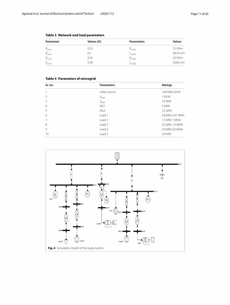
Table 3 Network and load parameters

Parameter Values (Ω) Parameters Values

RLine1 0.23 RLoad1 25 Ohm

XLine1 0.1 LLoad2 38.54 mH

RLine2 0.35 RLoad1 20 Ohm

XLine2 0.58 LLoad2 30.83 mH

Table 4 Parameters of microgrid

Sr. no. Parameters Ratings

1 Utility source 100 MVA, 69 kV

2 Vbase 13.8 kV

3 Sbase 10 MVA

4 DG1 5 MVA

5 DG2 2.5 MVA

6 Load 1 0.8 MW, 0.47 MVAr

7 Load 2 1.5 MW, 1 MVAr

8 Load 3 3.2 MW, 1.9 MVAr

9 Load 4 0.9 MW, 0.6 MVAr

10 Load 5 0.9 MW

Fig. 4 Simulation model of the study system


where Amg is the state matrix of microgrid, AINV is the state matrix of inverter, RN is neutral resistance, ANET is the state matrix of network, ALOAD is state matrix of load, MNET matrix gives connecting lines into the network and MLOAD matrix gives connect-ing lines into the load.

It would not be reliable to consider only static load or only dynamic load while consid-ering small signal stability. The microgrid or any distributed generation is a combination of static loads and dynamic loads. For the above reason in this paper, we analyse the sta-bility of islanded microgrid with composite load. To study the effect of composite load on stability, following equation is formulated,

The effect of damping and inertia on stability is also taken into the account during the study.

ResultsThe test system as shown in Fig. 3 is taken from [18] with base kV of 13.8 kV and base MVA of 10 MVA.

(44)ALoad = ARL + AZIP + ADynamic

Table 5 Eigenvalues comparison for ZIP load, RL load, dynamic load and composite load model

Eigenvalues ZIP RL Dynamic Composite

Negative 6 5 26 15

Positive 0 0 0 1

Real 9 10 14 19

Complex 0 1 10 1

Zero 3 6 6 4

Total 18 22 56 40

Fig. 5 Pole zero location of eigenvalues for the static load


For experimental verification of the system, 10 kVA inverter is considered. The param-eter value of the inverter is listed in Table 1. In Table 1, the gain parameters Mp, Nq, Kpv, Kiv, Kpc, Kic and F are dimensionless. The initial value of the parameter of the consid-ered system is presented in Table 2. The parameter for the load and network is given in Table 3, while parameter of the considered microgrid is displayed in Table 4.

From Table 1, it is evident that the switching frequency of the proposed network is considered as 8 kHz. The higher value of the switching frequency gives wide control limit. The coupling inductance (Lc) is used to provide coupling impedance between inverter output and interconnection bus, for better voltage regulation. The current feed forward gain (F) is used to provide low output impedance. This model composed three micro-sources (DG1, DG2 and DG3), 5 loads (two induction motors, two RL and one

Fig. 6 The reactive power of DG source with increases in static load of 1%

Fig. 7 Pole zero location of eigenvalues for the dynamic load


ZIP). The simulation model of the study system is simulated in the Power System Analy-sis Toolbox of the MATLAB environment as shown in Fig. 4.

In the present research, we investigated the effect of load, damping and inertia of the microgrid system. The eigenvalues of the three types of the load namely static (RL Load), dynamic (Induction motor) and composite load appear in Table 5.

From Table 5, it is visible that the numbers of the eigenvalues of the dynamic load are more as compared to static load, i.e. the nature of load affects the number of eigenvalues. The natures of the load also affect the other parameter of system such as active power, reactive power and speed. These parameters are discussed in subsequent sections.

Fig. 8 The reactive power of DG source with increases in dynamic load of 1%

Fig. 9 Pole zero location of eigenvalues for the composite load


Effect of load

System with static load

With static load, numbers of the eigenvalues are very few. In the present case, the num-bers of negative eigenvalues are 5 as detected in Table 5. The pole zero representation of eigenvalues of the static load is shown in Fig. 5. Figure 5 shows that all the eigenvalues are located on the left hand side plane. It indicates that the parameter of static load not much affecting the stability. The reactive power of DG source with increases in static

Fig. 10 The reactive power of DG source with increases in composite load of 1%

Table 6 Effect of increase in composite load

Eigenvalues Normal load Increase in load by 10%

Negative 32 26

Positive 1 2

Real 34 14

Complex 0 10

Zero 1 6

Total 68 58

Table 7 Effect of damping on micro-grid with composite load

Eigenvalues ζ = 0 ζ = 1 ζ = 10 ζ = 100

Negative 15 15 19 19

Positive 2 0 0 0

Real 19 19 19 21

Complex 1 1 1 0

Zero 4 6 2 2

Total 41 41 41 41


load of 1% is exhibited in Fig. 6. It is observed from Fig. 6 that after 5 s reactive power consumption of DG source is almost constant.

System with dynamic load

With a dynamic load like induction motor, the numbers of the eigenvalues are more because it considers both past as well as present data. Figure 7 gives the pole zero location of eigenvalues for the dynamic load. From Fig. 7, it is clear that the param-eter of dynamic load much affected the stability. Hence, during the planning of microgrid study the effect of induction motor is important.

The reactive power of DG source with increases in dynamic load of 1% is given in Fig. 8. From Fig. 8, it is clear that initially the speed of the motor is increasing so system is not more stable and it is oscillating up to 10 s. After 10 s, induction motor

Fig. 11 Pole zero plot of eigenvalues for the composite load with ζ = 0

Fig. 12 Pole zero plot of eigenvalues for the composite load with ζ = 1


speed is constant, so it is acting like static load. The reactive power consumption of the dynamic load is more as compared to the RL loads.

Fig. 13 Frequency of microgrid system with ζ = 0

Fig. 14 Frequency of microgrid system with ζ = 1

Table 8 Inertia affecting on system operation

Eigenvalues H = 3 H = 5.8 H = 7

Negative 13 15 16

Positive 2 1 0

Real 19 19 11

Complex 1 2 5

Zero 5 24 5

Total 21 21 21


System with composite load

With composite load, the numbers of eigenvalues are 40 as presented in Table 5. It is seen from Table 5 that one of the eigenvalues of the composite load is located on the right hand side plane, which make system towards instability and too much unhealthy for microgrid performance. The pole zeroes location of eigenvalues of the compos-ite load are shown in Fig. 9. The eigenvalue with red colour in Fig. 9 shows the posi-tive eigenvalue that moves the system towards instability. The consumption of reactive power at DG source with composite load is shown in Fig. 10. It is observed from Fig. 10 that reactive power consumption of composite load is increased and it is constant after 10 s.

The effect of increases of load by 10%, on the eigenvalues and stability, is demonstrated in Table 6. It is visible from Table 6 that as when the load is increased by 10%, the num-bers of positive eigenvalues are increased from 1 to 2 as compared to normal load. The increases in positive eigenvalues make the system more unstable. It indicates that if the composite load increases, microgrid system is moving towards instability.

Effect of damping

The performance of microgrid system with different value of damping is presented in Table 7. From Table 7, it is clear that when ζ = 0, two poles of the system are lying on the right hand side plane, while when ζ > 1, none of the poles lie on the right hand side plane.

The pole zeroes plots of the eigenvalues for the composite load with ζ = 0 and ζ = 1 are presented in Figs. 11 and 12, respectively. From Fig. 11, it is visible that when damping of the system is zero, one of the eigenvalue is located on the right hand side plane and makes the system unstable. From Fig. 12, it is investigated that when the damping of the system is one, all the eigenvalue of microgrid system are lying on the left hand side of the plane and system is more stable. From the above discussion, it is clear that as the damping of the system is increased from ζ = 0 to ζ = 1, stability of the system is increasing.

The frequency plot of the microgrid system with ζ = 0 and ζ = 1 is presented in Figs. 13 and 14, respectively. It is seen from Fig. 13 that system stables after 15 s. Also from Fig. 14, it is clear that system frequency is stable before 10 s. From the above discussion, it is observed that the damping of the system is increased, fre-quency oscillation is decreased.

Effect of inertia (H)

As we know that the main power system has rotating part, so it has more inertia, but in the present study, we consider microgrid with static devices so there is less inertia. The inertia can be increased by using switching FACT devices in the system. In this present work, we consider three different values of inertia as 3, 5.8 and 7 as shown in Table 8. Table 8 shows that the stability of microgrid system is increased if inertia is increased from 3 to 7.


ConclusionA complete state space model of microgrid with inverter dynamics, network dynamics and load dynamics is presented in this paper. All these three parts of microgrid are indi-vidually modelled and transferred to a common reference frame. During the planning of microgrid, it is necessary to consider the effects of the load parameters on the stability of microgrid hence here in this paper complete load modelling is carried out. The effect of dynamic and composite load parameters on the stability of the microgrid is considered and presented in the paper. The active and reactive power consumption of the microgrid system is different for the RL load, dynamic load and composite load. From the results, it is apparent that dynamic load and the composite load affect system stability more as compared to RL Load. Damping and inertia also affect the stability of the system. From the outcome, it is apparent that the stability of the microgrid system is increased when damping and inertia are increasing. The paper also presented the detail analysis of pole zero location for all the considered parameter. Hence, small signal stability analysis is most important for microgrid system for reliable operation of the power system. Com-pensation techniques can also be used to investigate its effect on stability and to locate compensator at proper place optimization techniques can be used. The hardware experi-mental setup will be developed for the simulation model of the test system for further study and validation of the results.

AbbreviationsSRF: synchronous reference frame; PCC: point of common coupling; CPL: constant power load; ZIP: constant impedance, current and power load; P: active power; Q: reactive power.

AcknowledgementsThe First authors would like to thank the Department of Electrical and Electronics Engineering, Sandip University Nashik (M.S.), India for providing the necessary help and support for preparing this paper. The Second author would also like to show her gratitude to the Department of Electrical Engineering S. B. Patil College of Engineering Indapur, Pune (M.S.), India for sharing their pearls of wisdom with her during the course of this research.

Authors’ contributionsAB conducted literature review, interpretation of the data and provide the resources for the paper, RA and CDD con-ducted mathematical modeling, implementation of the simulation model in the MATLAB environment and wrote the paper. All authors read and approved the final manuscript.

FundingNot applicable.

Availability of data and materialsAll authors confirm that all relevant data are included in the article in the section 4 from Table 1 to Table 4.

Competing interestsNot applicable.

Author details1 Department of Electrical Engineering, Sandip University, Nashik, MH, India. 2 Department of Electrical Engineering, SBPCOE, Indapur, MH, India. 3 Department of Electrical Engineering, PICT, Pune, MH, India.

Received: 25 January 2020 Accepted: 23 June 2020

References 1. Aboul-Seoud T, Jatskevich J (2008) Dynamic modeling of induction motor loads for transient voltage stability stud-

ies. In: IEEE conference on electric power conference, pp 1–5 2. Wong KE, Haque E (2014) Dynamic load modelling of a paper mill for small signal stability studies. IEEE Conf IET

Gener Transm Distrib 8(1):131–141 3. Ju P, Wu F, Shao ZY, Zhang XP, Fu HJ (2007) Composite load models based on field measurements and their applica-

tions in dynamic analysis. IET Gener Transm Distrib 1(5):724–730


4. Jili W, Renmu H, Jin M (2007) Load modeling considering distributed generation. In: IEEE conference on Power Technology, pp 1072–1077

5. Chandorkar MC, Divan DM, Adapa R (1993) Control of parallel connected inverters in standalone AC supply systems. IEEE Trans Ind Appl 29(1):136–143

6. Arriyasinghe DP, Vilathgamuwa DM (2008) Stability Analysis of microgrids with constant power loads. In: IEEE inter-national conference on sustainable energy technologies, pp 279–284

7. Liu Jianzhe, Zhang Wei, Rizzoni Giorgio (2018) Robust stability analysis of DC microgrids with constant power loads. IEEE Trans Power Syst 33(1):851–860

8. Hossain Eklas, Perez Ron, Nasiri Adel, Bayindir Ramazan (2018) Stability improvement of microgrids in the presence of constant power loads. Electr Power Energy Syst 96:442–456

9. Amelian SM, Hooshmand R (2013) Small signal stability analysis of microgrids considering comprehensive load models: a sensitivity based approach. In: IEEE smart grid conference (SGC), Tehran, pp 143–149

10. Kahrobaeian A, Yasser AR (2013) Stability analysis and control of medium-voltage micro-grids with dynamic loads. In: IEEE power and energy society general meeting, pp 1–5

11. Diaz Guzman, Gonzalez-Moran Cristina, Gomez-Aleixandre Javier, Diez Alberto (2010) Composite loads in stand-alone inverter- based microgrids modeling procedure and effects on load margin. IEEE Trans Power Syst 25(2):894–905

12. Kallamadi M, Sarkar V (2016) Generalised analytical framework for the stability studies of an AC microgrid. J Eng 2016:1–9

13. Pogaku N, Prodanovic M, Green TC (2007) Modeling, analysis and testing of autonomous operation of an inverter-based microgrid. IEEE Trans Power Electron 22(2):613–625

14. Abd-el-Motaleb AM, Hamilton D (2015) Modelling and sensitivity analysis of isolated microgrids. Renew Sustain Energy Rev 47:416–426

15. Martins N (1986) Efficient eigen value and frequency response methods applied to power system small-signal stability studies. In: IEEE power engineering review, vol PER-6, no 2, pp 47–47

16. Guan Y, Vasquez YC, Guerrero JM, Coelho EAA (2015) Small-signal modeling, analysis and testing of parallel three-phase-inverters with a novel autonomous current sharing controller. In: 2015 IEEE applied power electronics confer-ence and exposition (APEC), Charlotte, NC, pp 571–578

17. IEEE Task Force on Load Representation for Dynamic Performance (1995) Standard load models for power flow and dynamic performance simulation. In: IEEE transactions on power systems, vol 10, no 3, pp 1302–1313

18. Katiraei F, Iravani MR, Lehn PW (2005) Micro-grid autonomous operation during and subsequent to islanding pro-cess. IEEE Trans Power Deliv 20(1):248–257

19. Valdivia V, Diaz D, Gonzalez-Espin F, Foley R, Chang NC (2014) Systematic small signal modeling and stability analysis of a microgrid. In: IEEE 5th international symposium on power electronics for distributed generation systems (PEDG)

20. Shen L, Qiao W, Song R (2016) Characteristics and control strategies of composite energy storages in microgrids. In: China international conference on electricity distribution

21. Kamh MZ, Iravani R (2012) A sequence frame-based distributed slack bus model for energy management of active distribution networks. In: IEEE transactions on smart grid, vol 3, no 2

22. Zhao F, Li N, Yin Z, Tang X (2014) Small-signal modeling and stability analysis of DC microgrid with multiple type of loads. In: International conference on power system technology

23. Shi H, Zhuo F, Hou L, Yue X, Zhang D (2013) Small-signal stability analysis of a microgrid operating in droop control mode. In: IEEE ECCE Asia Downunder

Publisher’s NoteSpringer Nature remains neutral with regard to jurisdictional claims in published maps and institutional affiliations.

Documents

Small signal stability analysis of stand-alone microgrid