1

Small area estimates of consumption poverty in Croatia: methodological report

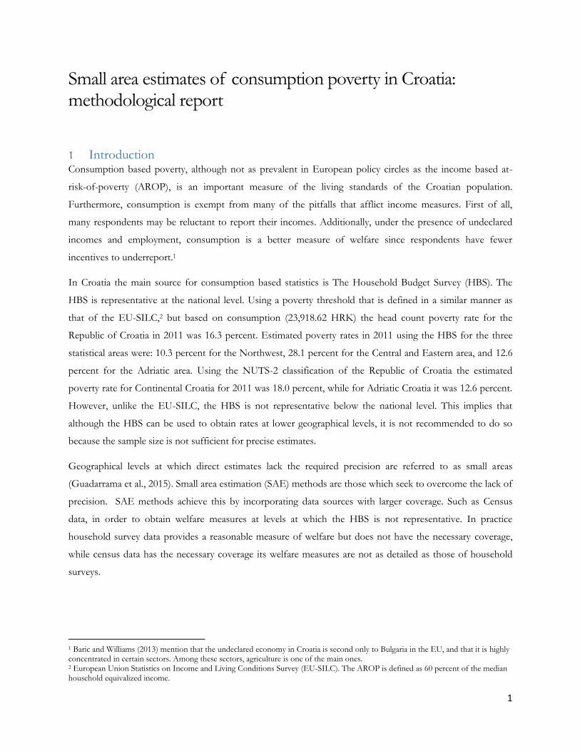
1 Introduction

Consumption based poverty, although not as prevalent in European policy circles as the income based at-

risk-of-poverty (AROP), is an important measure of the living standards of the Croatian population.

Furthermore, consumption is exempt from many of the pitfalls that afflict income measures. First of all,

many respondents may be reluctant to report their incomes. Additionally, under the presence of undeclared

incomes and employment, consumption is a better measure of welfare since respondents have fewer

incentives to underreport.1

In Croatia the main source for consumption based statistics is The Household Budget Survey (HBS). The

HBS is representative at the national level. Using a poverty threshold that is defined in a similar manner as

that of the EU-SILC,2 but based on consumption (23,918.62 HRK) the head count poverty rate for the

Republic of Croatia in 2011 was 16.3 percent. Estimated poverty rates in 2011 using the HBS for the three

statistical areas were: 10.3 percent for the Northwest, 28.1 percent for the Central and Eastern area, and 12.6

percent for the Adriatic area. Using the NUTS-2 classification of the Republic of Croatia the estimated

poverty rate for Continental Croatia for 2011 was 18.0 percent, while for Adriatic Croatia it was 12.6 percent.

However, unlike the EU-SILC, the HBS is not representative below the national level. This implies that

although the HBS can be used to obtain rates at lower geographical levels, it is not recommended to do so

because the sample size is not sufficient for precise estimates.

Geographical levels at which direct estimates lack the required precision are referred to as small areas

(Guadarrama et al., 2015). Small area estimation (SAE) methods are those which seek to overcome the lack of

precision. SAE methods achieve this by incorporating data sources with larger coverage. Such as Census

data, in order to obtain welfare measures at levels at which the HBS is not representative. In practice

household survey data provides a reasonable measure of welfare but does not have the necessary coverage,

while census data has the necessary coverage its welfare measures are not as detailed as those of household

surveys.

1 Baric and Williams (2013) mention that the undeclared economy in Croatia is second only to Bulgaria in the EU, and that it is highly concentrated in certain sectors. Among these sectors, agriculture is one of the main ones. 2 European Union Statistics on Income and Living Conditions Survey (EU-SILC). The AROP is defined as 60 percent of the median household equivalized income.

2

Figure 1: HBS 2011 poverty at level of representativeness

Republic of Croatia

The Census of Population, Households and Dwellings of 2011 for the Republic of Croatia when combined

with the 2011 HBS facilitates the estimation of welfare for all households in the Census. This makes obtaining

poverty rates for areas below those of the HBS’s representativeness possible. The small area estimation

methodology used to obtain the estimates follows the one proposed by Elbers, Lanjouw, and Lanjouw (ELL)

(2003).3 The methodology is perhaps the most widely used for small area estimation, and has been applied to

develop poverty maps in numerous countries across the globe. Through the application of the analysis,

predicted poverty rates at the NUTS-2,4 NUTS-3,5 as well as at the LAU-26 levels are obtained.

3 The methodology is implemented via the World Bank developed software PovMap (accessed on August 1, 2016) 4 Presently there are 2 spatial units under the NUTS 2 level, Adriatic and Continental Croatia. At the time of the 2011 HBS there were

three statistical areas in Croatia: Northwest, Central and Eastern, and Adriatic Croatia. 5 There are currently 21 spatial units at NUTS-3 level (Counties) in Croatia 6 There are 556 Local Administrative Units at level 2 (LAU 2). In Croatia LAU-2 level corresponds to municipalities and cities. Additionally, for the purposes of the analysis, the city of Zagreb is sub-divided into 19 districts.

3

2 Modeling approach

The ELL method is conducted in 2 stages. The first stage consists in fitting a welfare model using the 2011

HBS data via ordinary least squares (OLS), and correcting for various shortcomings of this approach to arrive

at generalized least squares estimates (GLS). It should be noted that the variables included in the welfare

model of the 2011 HBS must be restricted to those variables that are also found on the 2011 Census. This

allows us to generate the welfare distribution for any sub-population in the 2011 Census, conditional on the

sub-population’s observed characteristics (ELL, 2002).

After correcting for shortcomings, the estimated regression parameters, standard errors, and variance

components from the HBS provide the necessary inputs for the second phase of the analysis. The second

stage of the poverty mapping exercise consists in using the estimated parameters from the first stage, and

applying these to the 2011 Census data in order to predict welfare at the household level. Finally, the

predicted welfare measure is converted into a poverty indicator which is then aggregated in order to predict

poverty measures at the desired level of aggregation (NUTS2, NUTS3, or LAU2).

Before fitting the welfare model, a comparison between the observable household characteristics from the

HBS and the census is necessary. The purpose of the comparison is to ensure that variables have similar

distributions, and that these have similar definitions across data sources. Because the exercise consists in

predicting welfare in the census data using parameters obtained from HBS observed characteristics it is

imperative that the observed characteristics across surveys are comparable.

The next step in the ELL methodology consists in estimating a log adult equivalized household consumption

model which is estimated via OLS. The transformation to log consumption is done because consumption

tends to not be symmetrically distributed (graph 1), taking the logarithm of consumption is done to make the

data more symmetrical.

Figure 2: Adult equivalized consumption and natural logarithm of adult equivalized consumption

4

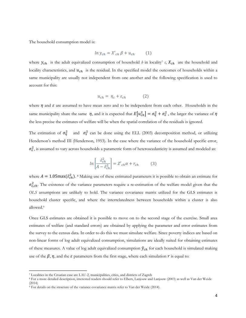
The household consumption model is:

𝑙𝑛 𝑦𝑐ℎ = 𝑋′𝑐ℎ 𝛽 + 𝑢𝑐ℎ (1)

where 𝑦𝑐ℎ is the adult equivalized consumption of household h in locality7 c, 𝑋𝑐ℎ are the household and

locality characteristics, and 𝑢𝑐ℎ is the residual. In the specified model the outcomes of households within a

same municipality are usually not independent from one another and the following specification is used to

account for this:

𝑢𝑐ℎ = 𝜂𝑐 + 𝜀𝑐ℎ (2)

where 𝜂 and 𝜀 are assumed to have mean zero and to be independent from each other. Households in the

same municipality share the same 𝜂, and it is expected that 𝐸[𝑢𝑐ℎ2 ] = 𝜎𝜂

2 + 𝜎𝜀2 , the larger the variance of 𝜂

the less precise the estimates of welfare will be when the spatial correlation of the residuals is ignored.

The estimation of 𝜎𝜂2 and 𝜎𝜀

2 can be done using the ELL (2003) decomposition method, or utilizing

Henderson’s method III (Henderson, 1953). In the case where the variance of the household specific error,

𝜎𝜀2, is assumed to vary across households a parametric form of heteroscedasticity is assumed and modeled as:

𝑙𝑛 [𝜀��ℎ

2

𝐴 − 𝜀��ℎ2 ] = 𝑍′𝑐ℎ𝛼 + 𝑟𝑐ℎ (3)

where 𝐴 = 1.05max (𝜀��ℎ2 ). 8 Making use of these estimated parameters it is possible to obtain an estimate for

𝜎𝜀,𝑐ℎ2 . The existence of the variance parameters require a re-estimation of the welfare model given that the

OLS assumptions are unlikely to hold. The variance covariance matrix utilized for the GLS estimates is

household cluster specific, and where the interrelatedness between households within a cluster is also

allowed.9

Once GLS estimates are obtained it is possible to move on to the second stage of the exercise. Small area

estimates of welfare (and standard errors) are obtained by applying the parameter and error estimates from

the survey to the census data. In order to do this we must simulate welfare. Since poverty indices are based on

non-linear forms of log adult equivalized consumption, simulations are ideally suited for obtaining estimates

of these measures. A value of log adult equivalized consumption ��𝑐ℎ for each household is simulated making

use of the 𝛽, 𝜂, and the 𝜀 parameters from the first stage, where each simulation 𝑟 is equal to:

7 Localities in the Croatian case are LAU-2, municipalities, cities, and districts of Zagreb 8 For a more detailed description, interested readers should refer to Elbers, Lanjouw and Lanjouw (2003) as well as Van der Weide (2014) 9 For details on the structure of the variance covariance matrix refer to Van der Weide (2014).

5

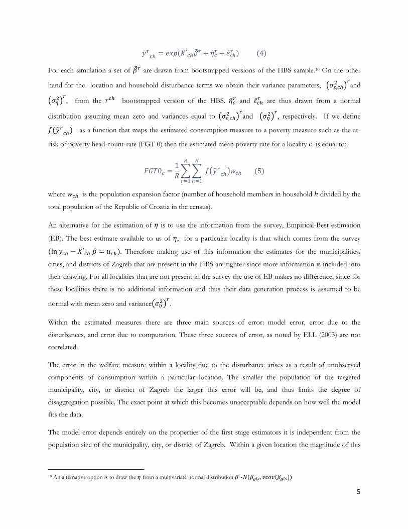
��𝑟𝑐ℎ = 𝑒𝑥𝑝(𝑋′𝑐ℎ��𝑟 + ��𝑐

𝑟 + 𝜀��ℎ𝑟 ) (4)

For each simulation a set of ��𝑟 are drawn from bootstrapped versions of the HBS sample.10 On the other

hand for the location and household disturbance terms we obtain their variance parameters, (𝜎𝜀,𝑐ℎ2 )

𝑟and

(𝜎𝜂2)

𝑟, from the 𝑟𝑡ℎ bootstrapped version of the HBS. ��𝑐

𝑟 and 𝜀��ℎ𝑟 are thus drawn from a normal

distribution assuming mean zero and variances equal to (𝜎𝜀,𝑐ℎ2 )

𝑟and (𝜎𝜂

2)𝑟, respectively. If we define

𝑓(��𝑟𝑐ℎ) as a function that maps the estimated consumption measure to a poverty measure such as the at-

risk of poverty head-count-rate (FGT 0) then the estimated mean poverty rate for a locality 𝑐 is equal to:

𝐹𝐺𝑇0𝑐 =1

𝑅∑ ∑ 𝑓(��𝑟

𝑐ℎ)𝑤𝑐ℎ

𝐻

ℎ=1

𝑅

𝑟=1

(5)

where 𝑤𝑐ℎ is the population expansion factor (number of household members in household ℎ divided by the

total population of the Republic of Croatia in the census).

An alternative for the estimation of 𝜂 is to use the information from the survey, Empirical-Best estimation

(EB). The best estimate available to us of 𝜂, for a particular locality is that which comes from the survey

(ln 𝑦𝑐ℎ − 𝑋′𝑐ℎ 𝛽 = 𝑢𝑐ℎ). Therefore making use of this information the estimates for the municipalities,

cities, and districts of Zagreb that are present in the HBS are tighter since more information is included into

their drawing. For all localities that are not present in the survey the use of EB makes no difference, since for

these localities there is no additional information and thus their data generation process is assumed to be

normal with mean zero and variance(𝜎𝜂2)

𝑟.

Within the estimated measures there are three main sources of error: model error, error due to the

disturbances, and error due to computation. These three sources of error, as noted by ELL (2003) are not

correlated.

The error in the welfare measure within a locality due to the disturbance arises as a result of unobserved

components of consumption within a particular location. The smaller the population of the targeted

municipality, city, or district of Zagreb the larger this error will be, and thus limits the degree of

disaggregation possible. The exact point at which this becomes unacceptable depends on how well the model

fits the data.

The model error depends entirely on the properties of the first stage estimators it is independent from the

population size of the municipality, city, or district of Zagreb. Within a given location the magnitude of this

10 An alternative option is to draw the 𝜂 from a multivariate normal distribution 𝛽~𝑁(𝛽𝑔𝑙𝑠, 𝑣𝑐𝑜𝑣(𝛽𝑔𝑙𝑠))

6

error component will also depend on how different the 𝑋 variables are in that location from those of the

HBS data.

Finally, computation error is due to the method used for computation. This error can be made as small as

needed depending on the computational resources at hand. Because often simulations are a finite number, the

larger the number of simulations, the smaller the error due to computation will be.

3 Data description

The poverty mapping analysis requires two sources of data. In this instance the Croatian Household Budget

Survey (HBS) for 2011, and the Census of Population, Households and Dwellings of 2011 for the Republic

of Croatia. The HBS for 2011 is an ideal household survey for the SAE analysis because it corresponds to the

2011 calendar year, and thus are for the same time period as the census.

Small area estimation is done under the assumption that the same underlying population is being captured by

the survey and the census. This last assumption will be valid if both datasets are from the same time frame.

Nevertheless, the inclusion or the use of datasets that are from differing time periods, or if the survey is not

representative of the population, will break down this assumption. This last remark is more salient in

instances where there have been considerable shocks in between the collection of the survey and the

collection of the census (Bedi et al. 2007).

3.1 HBS 2011 – Croatia

The Household Budget Survey conducted by the Croatian Bureau of Statistics is collected over 12 months,

corresponding to the calendar year. The survey collects data on the socio-economic characteristics of

Croatian private households, along with household consumption, and income. The data collected is used to

update the weights of the national consumer price index and the measurement of household consumption, as

well as for the needs of national accounts.

The 2011 HBS uses the 2001 Census as a sampling frame. The survey is performed as a two-stage sample,

where 10 dwellings were selected from 416 segments (groups of neighboring enumeration areas).

Consequently, 4,160 dwellings occupied by households were selected. From these households, 2,335 were

successfully interviewed.

The Republic of Croatia does not currently have any poverty measures based on consumption. As a

consequence, the same methodology applied to the EU-SILC is used but in this instance on consumption.

7

More explicitly, the at-risk-of-poverty threshold is defined as 60 percent of the median household equivalized

consumption.

3.2 Census of Population, Households and Dwellings 2011, Population by Sex and Age

The 2011 Census for Croatia was provided by the Croatian Bureau of Statistics.11 The census includes key

information on demographics of the household, education, labor force status, economic activity, occupation

type, and labor status in the main job. Along with these characteristics, the census also has information on the

type of dwelling, the status of the dwelling, number of rooms in the dwelling, living area of the dwelling, and

the construction year.

3.3 Variable comparison between HBS and Census

Because small area methods require an estimation of a welfare model in the first stage which will then be

applied to the census it is necessary that the choice of correlates matches across surveys. This not only

requires variables to be similar, but requires that these have similar distributions. The selection of candidate

variable is done in a two stage process:

1. Comparison of questionnaires between the 2011 HBS and the 2011 Census. The comparison yields a

first set of candidate variables for the estimation. Candidate variables must come from similar

questions.

2. Comparison of the distribution of the candidate variables across datasets. The comparison is

undertaken at the level of the Republic of Croatia and at the statistical region level. The comparability

of the variables across surveys ensures that the welfare model from the 2011 HBS can be applied to

the 2011 Census such that reliable consumption estimates for the population can be derived.

Making use of all variables that meet the above criteria, several welfare models are estimated via OLS. Unlike

most of econometrics, the purpose of the model is not to find any causal relationships but to find a model

that best reflects the consumption level of a household. The adult equivalized consumption of a household is

assumed to be a function of the number of household members present in the household, and the age

composition of the household members. Additionally, consumption is assumed to be a function of the

marital status of individuals aged 15 and over, their level of education, their occupation, and the sector in

which they are employed in. In addition, and while likely not a determinant of consumption, we include a

11 Access to the Census, as well as the HBS was provided in the Croatian Bureaus of Statistics’ saferoom with excluded direct identifiers for individuals.

8

variable which reports the area of the dwelling in square meters. This variable is expected to have reasonable

correlation with welfare. Finally, the use of location means of household level variables are included.12 This is

done in order to explain the variation in welfare due to location as much as possible and thus improve

precision of the welfare estimates.

Table 1 contains a listing of the candidate variables for use in the model. Given that the sampling frame for

the 2011 HBS is the previous Census (Census of Population, Households and Dwellings 2001) it is not

unexpected that the first moments of the HBS and Census are somewhat different. On population

demographics, the differences between the two are slight, but on labor characteristics differences do arise.

For example, the HBS contains a larger share individuals living in households where one of the household

members is involved in agriculture, mining or fishing.

Table 1: Population weighted candidate variable means in Census 2011 and HBS-2011

Variable name Census 2011 HBS-2011

Male share of population 0.483 0.466

Age [0,5) 0.050 0.036

Age [5,15) 0.103 0.093

Age [15,30) 0.186 0.190

Age [30,65) 0.486 0.480

Age [65+) 0.174 0.202

Household size (Share of individuals living in household type)

Households size of 1 0.088 0.084

Households size of 2 0.183 0.222

Households size of 3 0.202 0.180

Households size of 4 0.248 0.223

Households size of 5 0.143 0.156

Households size of 6 0.076 0.077

Household size of 7 or more 0.060 0.057

Occupation (15+) (Share of individuals in households with at least one member)

Manager 0.051 0.034

Professionals 0.150 0.110

Technicians 0.182 0.137

Clerical support 0.129 0.130

Service and sales 0.223 0.194

Skilled agriculture 0.041 0.086

Craft and trade 0.153 0.170

12

This is recommended by ELL (2003) as one method to decrease the variance of 𝜂 since it includes more information at the cluster level. Variable means at the municipal level are included and come from the Census. These are the share of households in the municipality, city, or district of Zagreb that were built between 1900 and 1940, share of household that have air conditioning, and the proportion of households that have never moved out of their municipality, city, or district of Zagreb.

9

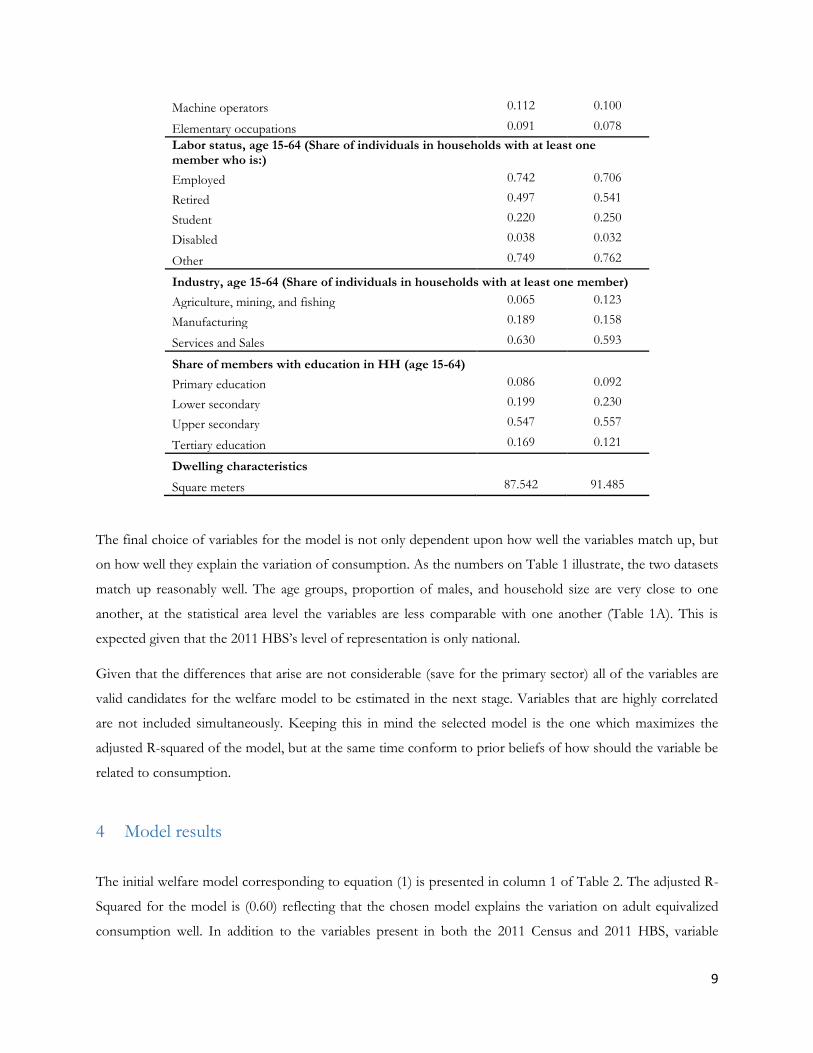
Machine operators 0.112 0.100

Elementary occupations 0.091 0.078

Labor status, age 15-64 (Share of individuals in households with at least one member who is:)

Employed 0.742 0.706

Retired 0.497 0.541

Student 0.220 0.250

Disabled 0.038 0.032

Other 0.749 0.762

Industry, age 15-64 (Share of individuals in households with at least one member)

Agriculture, mining, and fishing 0.065 0.123

Manufacturing 0.189 0.158

Services and Sales 0.630 0.593

Share of members with education in HH (age 15-64)

Primary education 0.086 0.092

Lower secondary 0.199 0.230

Upper secondary 0.547 0.557

Tertiary education 0.169 0.121

Dwelling characteristics Square meters 87.542 91.485

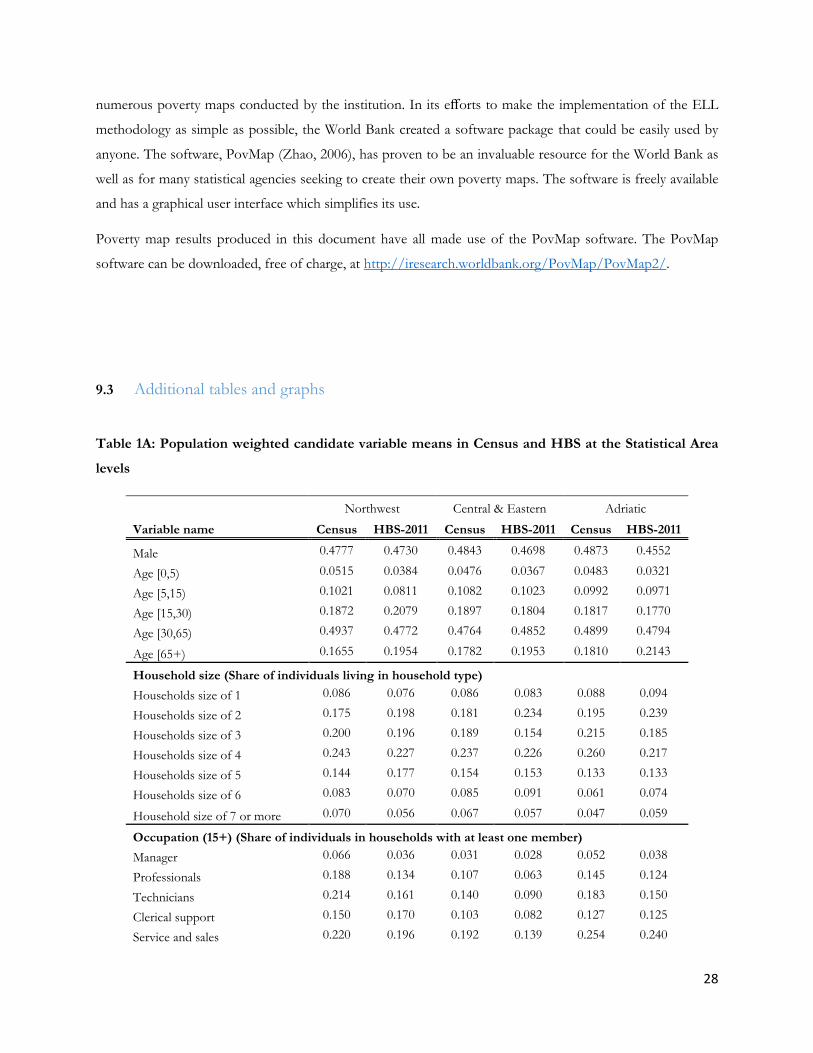
The final choice of variables for the model is not only dependent upon how well the variables match up, but

on how well they explain the variation of consumption. As the numbers on Table 1 illustrate, the two datasets

match up reasonably well. The age groups, proportion of males, and household size are very close to one

another, at the statistical area level the variables are less comparable with one another (Table 1A). This is

expected given that the 2011 HBS’s level of representation is only national.

Given that the differences that arise are not considerable (save for the primary sector) all of the variables are

valid candidates for the welfare model to be estimated in the next stage. Variables that are highly correlated

are not included simultaneously. Keeping this in mind the selected model is the one which maximizes the

adjusted R-squared of the model, but at the same time conform to prior beliefs of how should the variable be

related to consumption.

4 Model results

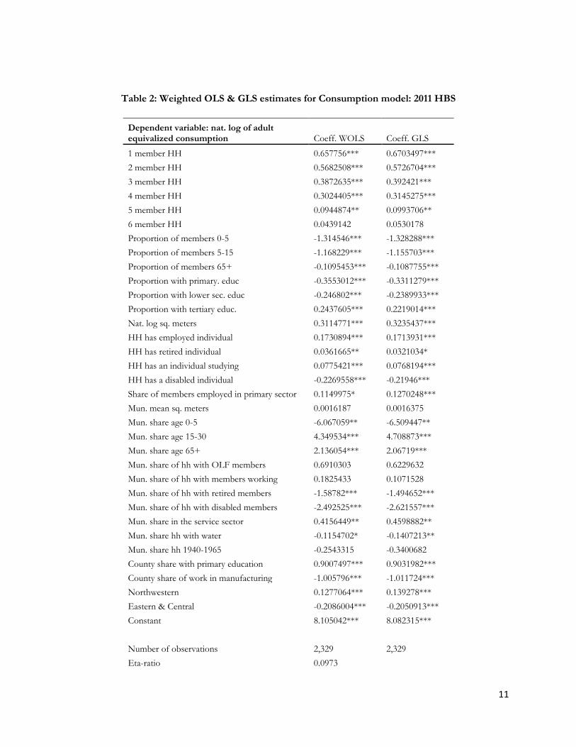
The initial welfare model corresponding to equation (1) is presented in column 1 of Table 2. The adjusted R-

Squared for the model is (0.60) reflecting that the chosen model explains the variation on adult equivalized

consumption well. In addition to the variables present in both the 2011 Census and 2011 HBS, variable

10

means for municipalities are obtained from the Census and introduced to the model; these variables are

introduced to improve precision by reducing the unexplained variation in adult equivalized consumption due

to location. The same is done at the NUTS-3 level. With the inclusion of these variables the ratio of the

variance of 𝜂 over the model’s MSE is 0.097. Without the inclusion of the regional means, the variance of 𝜂

over the model’s MSE was considerably larger (greater than 0.16). The variance of the location effect is

preferred to be small, this will result in more precise estimates once the parameters are applied to the Census

when predicting consumption.

As noted in section 2, it is likely that consumption levels within a location are highly correlated and as a

consequence 𝐸[𝑢𝑐ℎ𝑢𝑐𝑖|𝑋] ≠ 0. Additionally, error terms will likely have differing variances across

observations (𝐸[𝑢𝑐ℎ2 |𝑋] ≠ 𝜎2). Due to these issues the model is re-estimated using Generalized Least

Squares (GLS). The results for the GLS fitted model are presented in column 2 of Table 2.13

Adult equivalized consumption is positively correlated to household size. The omitted group is households

with 7 or more individuals. Furthermore, adult equivalized consumption is negatively correlated to greater

proportion of young children in the household, as opposed to individuals between 15 and 65. A higher

proportion of elderly household members is also negatively related to consumption.

Education is also significantly related to consumption. The omitted group is the proportion of working age

household members who have upper-secondary education. As expected, a higher share of more educated

working age members is positively and significantly related to adult equivalized consumption. Also correlated

to consumption is the presence of employed individuals, additionally most of the labor variables included are

significantly correlated to adult equivalized consumption.

Location and location variable means are also correlated to adult equivalized consumption. Consumption is

negatively correlated to being located in the Central and Eastern statistical region of Croatia as opposed to

being in the Adriatic. On the other hand residing in the Northwest statistical region is positively and

significantly correlated to adult equivalized consumption. The Continental NUTS-2 region is made up of the

Northwest and the Central Eastern statistical regions. The opposite signs for the two statistical regions,

present evidence of an existing difference within the Continental NUTS-2 spatial unit.

13 The alpha model (equation 3) corresponding to the GLS are presented in Table 2A.

11

Table 2: Weighted OLS & GLS estimates for Consumption model: 2011 HBS

Dependent variable: nat. log of adult equivalized consumption Coeff. WOLS Coeff. GLS

1 member HH 0.657756*** 0.6703497***

2 member HH 0.5682508*** 0.5726704***

3 member HH 0.3872635*** 0.392421***

4 member HH 0.3024405*** 0.3145275***

5 member HH 0.0944874** 0.0993706**

6 member HH 0.0439142 0.0530178

Proportion of members 0-5 -1.314546*** -1.328288***

Proportion of members 5-15 -1.168229*** -1.155703***

Proportion of members 65+ -0.1095453*** -0.1087755***

Proportion with primary. educ -0.3553012*** -0.3311279***

Proportion with lower sec. educ -0.246802*** -0.2389933***

Proportion with tertiary educ. 0.2437605*** 0.2219014***

Nat. log sq. meters 0.3114771*** 0.3235437***

HH has employed individual 0.1730894*** 0.1713931***

HH has retired individual 0.0361665** 0.0321034*

HH has an individual studying 0.0775421*** 0.0768194***

HH has a disabled individual -0.2269558*** -0.21946***

Share of members employed in primary sector 0.1149975* 0.1270248***

Mun. mean sq. meters 0.0016187 0.0016375

Mun. share age 0-5 -6.067059** -6.509447**

Mun. share age 15-30 4.349534*** 4.708873***

Mun. share age 65+ 2.136054*** 2.06719***

Mun. share of hh with OLF members 0.6910303 0.6229632

Mun. share of hh with members working 0.1825433 0.1071528

Mun. share of hh with retired members -1.58782*** -1.494652***

Mun. share of hh with disabled members -2.492525*** -2.621557***

Mun. share in the service sector 0.4156449** 0.4598882**

Mun. share hh with water -0.1154702* -0.1407213**

Mun. share hh 1940-1965 -0.2543315 -0.3400682

County share with primary education 0.9007497*** 0.9031982***

County share of work in manufacturing -1.005796*** -1.011724***

Northwestern 0.1277064*** 0.139278***

Eastern & Central -0.2086004*** -0.2050913***

Constant 8.105042*** 8.082315***

Number of observations 2,329 2,329

Eta-ratio 0.0973

12

Adjusted R-squared 0.5998 *, **, *** significant at the 10, 5, 1 percent level respectively. All households which have inconsistent labor information are removed.

5 Poverty results

The coefficients estimated in the previous section provide the necessary inputs in order to estimate the first

part of equation 4 (𝑋′𝑐ℎ��) by combining coefficients with the Census variables. The vectors of disturbances

for households are unknown, and must be estimated. As mentioned before, the error component is

decomposed using ELL’s method, and the coefficients, 𝛽, are obtained by bootstrapped samples of the 2011

HBS data. The model chosen is the one where 𝜂 and 𝜀 are drawn from a normal distribution, with their

respective variance structures. Finally, empirical best methods are chosen since these incorporate more

information and are thus expected to provide a better fit. Additionally, empirical best incorporates different

variance structures across locations which in many settings may be more believable.14

The clustering used for estimations is at the municipal, city, and districts of Zagreb level, the resulting poverty

map aggregated to the NUTS-3 level is presented in Figure 3 and the results for municipalities, cities, and the

districts of Zagreb are presented in Figure 4. The resulting poverty rates obtained at the statistical region level

compared to those of the poverty mapping exercise are presented in Table 3 for the relative line.

Table 3: Poverty rates from HBS and from poverty map exercise

Statistical region AROP HBS

HBS 95% CI Predicted 95% CI

Northwestern 10.3% 7.6% 13.7% 11.1% 9.5% 12.7%

Central & Eastern 28.1% 23.5% 33.3% 30.5% 28.4% 32.7%

Adriatic 12.6% 9.2% 17.0% 12.6% 11.0% 14.1%

Republic of Croatia 16.3% 14.1% 18.6% 17.1% 15.8% 18.5%

Note: Poverty threshold 23,918.62 HRK per adult equivalent

At the statistical area level, the direct estimates for poverty rates obtained from the HBS are not significantly

different. However, once again, it is important to note that the 2011 HBS measures of poverty for statistical

areas are not statistically representative. The same holds true for the NUTS-2 spatial units, the 2011 HBS is

not statistically representative below the national level. The direct estimate of poverty from the 2011 HBS for

14 This only applies to municipalities, cities, and districts of Zagreb included in the 2011 HBS.

13

Continental Croatia is 18.0 percent, and for Adriatic Croatia it is 12.6 percent. The small area estimate of

poverty for Continental Croatia is 19.4 percent, while for Adriatic Croatia it is 12.6 percent.

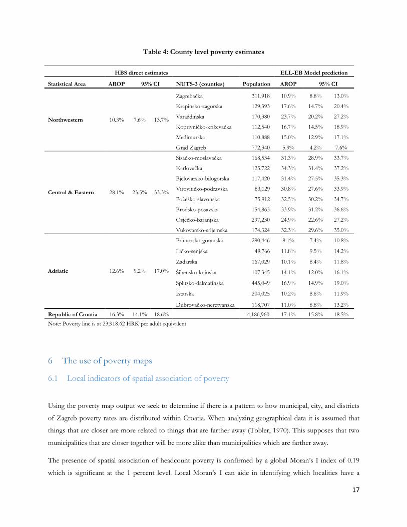
The Central and Eastern area has the highest levels of poverty, the poverty rate is significantly greater than

that of the other two areas. The headcount poverty rate for the Central and Eastern area is more than double

the level of the other two areas. Poverty ranges from 24.9 to 34.3 percent in the Central and Eastern statistical

region. In the Northwest statistical region, poverty ranges between 5.9 (Grad Zagreb) to 23.7 (Varaždinska)

percent. In the Adriatic the range is less wide from 9.1 for Primorsko-goranska to 16.9 for Splitsko-

dalmatinska. Furthermore, the Adriatic region has the most counties with poverty rates under 15 percent.

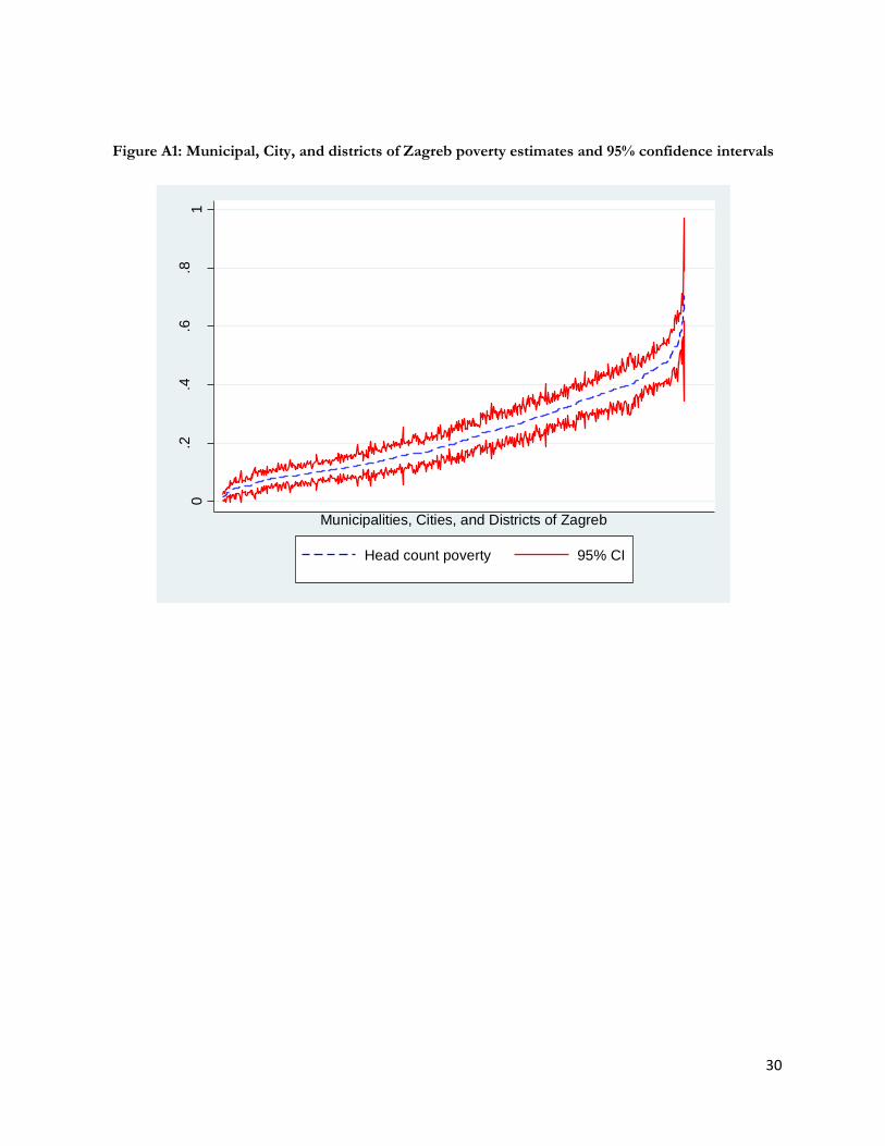
In Figure 4, which is at the municipal, city and districts of Zagreb level, it is possible to detect localities that

have a somewhat higher poverty level than its surroundings. There are some localities with high poverty rates

within the Northwest as well as in the Adriatic. In the Central & Eastern region, on the other hand, there are

some regions that are better off than their neighbors. The results of the poverty map suggest an overall

spatial clustering of poverty, this is further analyzed in section 6, where basic analysis of the spatial association

is undertaken.

Although poverty rates may be low in certain counties, the concentration of the poor may not be the lowest

in those counties. Figure 5 presents the density of the poor at the county level. One of the counties with the

highest concentration of poor individuals are Osječko-baranjska, this is despite having the lowest poverty

headcount in the Central and Eastern statistical area. The county with the highest share of poor individuals is

in the Adriatic part of the country, Splitsko-dalmatinska which also happens to be the country with the

highest poverty rate in the Adriatic. The city of Zagreb is also home to a considerable amount of Croatia’s

poor with close to 6.3 percent of the nation’s poor calling Zagreb home.

Figure 3: Poverty Map - NUTS-3 poverty headcount

14

15

Figure 4: Poverty Map - poverty headcount for municipalities, cities, and districts of Zagreb

16

Figure 5: Distribution of the poor by NUTS-3 spatial units

17

Table 4: County level poverty estimates

HBS direct estimates ELL-EB Model prediction

Statistical Area AROP 95% CI NUTS-3 (counties) Population AROP 95% CI

Northwestern 10.3% 7.6% 13.7%

Zagrebačka 311,918 10.9% 8.8% 13.0%

Krapinsko-zagorska 129,393 17.6% 14.7% 20.4%

Varaždinska 170,380 23.7% 20.2% 27.2%

Koprivničko-križevačka 112,540 16.7% 14.5% 18.9%

Međimurska 110,888 15.0% 12.9% 17.1%

Grad Zagreb 772,340 5.9% 4.2% 7.6%

Central & Eastern 28.1% 23.5% 33.3%

Sisačko-moslavačka 168,534 31.3% 28.9% 33.7%

Karlovačka 125,722 34.3% 31.4% 37.2%

Bjelovarsko-bilogorska 117,420 31.4% 27.5% 35.3%

Virovitičko-podravska 83,129 30.8% 27.6% 33.9%

Požeško-slavonska 75,912 32.5% 30.2% 34.7%

Brodsko-posavska 154,863 33.9% 31.2% 36.6%

Osječko-baranjska 297,230 24.9% 22.6% 27.2%

Vukovarsko-srijemska 174,324 32.3% 29.6% 35.0%

Adriatic 12.6% 9.2% 17.0%

Primorsko-goranska 290,446 9.1% 7.4% 10.8%

Ličko-senjska 49,766 11.8% 9.5% 14.2%

Zadarska 167,029 10.1% 8.4% 11.8%

Šibensko-kninska 107,345 14.1% 12.0% 16.1%

Splitsko-dalmatinska 445,049 16.9% 14.9% 19.0%

Istarska 204,025 10.2% 8.6% 11.9%

Dubrovačko-neretvanska 118,707 11.0% 8.8% 13.2%

Republic of Croatia 16.3% 14.1% 18.6% 4,186,960 17.1% 15.8% 18.5%

Note: Poverty line is at 23,918.62 HRK per adult equivalent

6 The use of poverty maps

6.1 Local indicators of spatial association of poverty

Using the poverty map output we seek to determine if there is a pattern to how municipal, city, and districts

of Zagreb poverty rates are distributed within Croatia. When analyzing geographical data it is assumed that

things that are closer are more related to things that are farther away (Tobler, 1970). This supposes that two

municipalities that are closer together will be more alike than municipalities which are farther away.

The presence of spatial association of headcount poverty is confirmed by a global Moran’s I index of 0.19

which is significant at the 1 percent level. Local Moran’s I can aide in identifying which localities have a

18

statistically significant relationship with its neighbors. Spatial autocorrelation makes the identification of high

poverty areas (particularly in the Central and Eastern statistical region), as well as low poverty areas (around

Zagreb and the surrounding areas of Istarska). Confirming the concentration of poverty in the Central and

Eastern statistical area of the country, the map in Figure 7 illustrates a massive hotspot of poverty in the area.

These results bring to light the challenges that arise for regional development, and add a new layer to the

discussion.

As noted in Section 5 and in Figure 4, there appears to be some spatial clustering in the results from the

poverty maps. In fact the Central and Eastern regions seem to be lagging behind the Adriatic and Northwest.

Poverty rates in Central and Eastern regions are considerably greater than the rest of the country, and the

region appears to be a hotspot for poverty. Furthermore, there appears to be a clear demarcation of low

versus high poverty areas. Insofar as determining if there is in fact spatial correlation we rely on Global

Moran’s I as well as Local Moran’s I statistic, and the Getis-Ord Gi, shown in Figure 6 and 7 respectively.

Figure 6 presents the results for the Global and Local Moran’s I statistics. The significant (Z-score of 57.8)

Global Moran’s I of 0.20 suggests that there is spatial autocorrelation. Additionally, the map illustrates regions

which are significantly different from their neighbors, and regions which are high-poverty areas and low

poverty areas. All colored areas show a significant relationship to their neighbors. Those municipalities

marked as “High – High” (“Low-Low”) are municipalities where poverty is significantly greater (lower) than

the neighborhood’s poverty and are greater (lower) than the average poverty among municipalities.

In order to obtain spatial statistics it is necessary to establish a degree of spatial proximity between the

municipalities in Croatia. A spatial weights matrix is used, which relies on the row-standardized inverse

distances between the center of the municipalities and the surrounding municipalities. This ensures that

nearer neighbors have a greater influence on the analyzed outcomes, in this instance poverty rates.

A cluster of high poverty is clearly delineated in the Eastern Central statistical area (Figure 6 and 7). In Zagreb

and surrounding areas a cluster of low poverty is highlighted, the same holds true for the north of the

Adriatic region. Municipalities marked as low-high outliers and the high-low outliers are particularly of

interest. While poverty may be high (low) in particular areas, there are some municipalities that have a

significantly lower (higher) level of poverty than its surroundings. These are mostly observed in the Adriatic

and Eastern Central areas.

The hot spot analysis in Figure 7, brings to light a demarcation and separation between regions. This was also

evident in the results from the OLS and GLS (see Table 2). All three statistical areas are different.

Independently from the NUTS-2 classification which aggregates the Northwestern statistical area and the

Eastern and Central statistical area, when it comes to welfare these areas are considerably different.

19

20

Figure 6: Poverty Map - Spatial association of headcount poverty

21

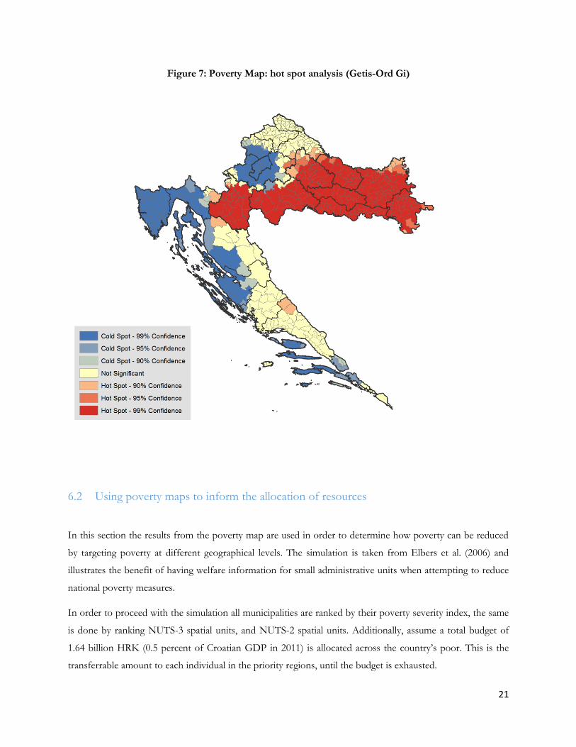
Figure 7: Poverty Map: hot spot analysis (Getis-Ord Gi)

6.2 Using poverty maps to inform the allocation of resources

In this section the results from the poverty map are used in order to determine how poverty can be reduced

by targeting poverty at different geographical levels. The simulation is taken from Elbers et al. (2006) and

illustrates the benefit of having welfare information for small administrative units when attempting to reduce

national poverty measures.

In order to proceed with the simulation all municipalities are ranked by their poverty severity index, the same

is done by ranking NUTS-3 spatial units, and NUTS-2 spatial units. Additionally, assume a total budget of

1.64 billion HRK (0.5 percent of Croatian GDP in 2011) is allocated across the country’s poor. This is the

transferrable amount to each individual in the priority regions, until the budget is exhausted.

22

The simulated transfer is independent of the individual’s status, everyone within the priority regions will

receive the same amount. When the transfer is assumed to be done uniformly across the country, the amount

transferred to each individual is the close to 390 HRK. When transferring at lower levels of aggregation, the

amount transferred to each individual is equal to the budget over the number of poor individuals in the

country. Therefore, every individual within the locality receives an equal amount of money regardless of

his/her poverty status. If the funds run out before all in the locality receive the same amount, the remaining

budget is split evenly amongst the individuals within that locality. Finally, it is assumed that the entire transfer

will be devoted to household consumption.

Since for the poverty maps 100 simulations have been performed we have 100 vectors of consumption for

each household. For each of these vectors the transfer amount is added to the household’s adult equivalized

consumption, irrespective if the household is poor in that particular simulation or not. The ranking of

locations is done on the final results of severity from the poverty maps, i.e. the mean of the severity rate for

each locality for all simulations. This type of targeting is referred to as “naïve” by Elbers et al. (2006). Since

the ranking is done on the final results, the transfer in each simulation is also independent on the location’s

ranking within that particular simulation.

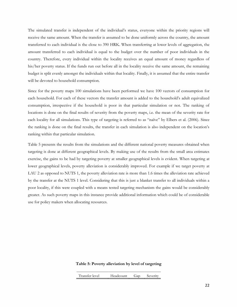
Table 5 presents the results from the simulations and the different national poverty measures obtained when

targeting is done at different geographical levels. By making use of the results from the small area estimates

exercise, the gains to be had by targeting poverty at smaller geographical levels is evident. When targeting at

lower geographical levels, poverty alleviation is considerably improved. For example if we target poverty at

LAU 2 as opposed to NUTS 1, the poverty alleviation rate is more than 1.6 times the alleviation rate achieved

by the transfer at the NUTS 1 level. Considering that this is just a blanket transfer to all individuals within a

poor locality, if this were coupled with a means tested targeting mechanism the gains would be considerably

greater. As such poverty maps in this instance provide additional information which could be of considerable

use for policy makers when allocating resources.

Table 5: Poverty alleviation by level of targeting

Transfer level Headcount Gap Severity

23

NUTS-1 (baseline) 1.00 1.00 1.00

NUTS-2 1.05 1.10 1.14

NUTS-3 1.50 1.66 1.70

Municipalities, cities, and districts of Zagreb

1.59 1.89 2.03

Note: Transfer is 1.64 billion HRK (0.5% of GDP)

24

7 Concluding remarks

Direct poverty estimates from the HBS are only reliable at the national level. This complicates the analysis of

poverty at more disaggregated levels since the reliability of direct estimates are questionable. Data from the

Census of Population, Households and Dwellings 2011 coupled with small area estimation techniques aide

policy makers in overcoming the lack of precision at lower geographical levels. The results from the poverty

mapping exercise, coupled with spatial analysis reveal the heterogeneity of poverty in Croatia.

Results from spatial analysis reveal that there is a cluster of high poverty in the Central and Eastern statistical

region of Croatia. There is a clear poverty demarcation in the country, where the Central and Eastern part of

the country is clearly doing worse than the rest of the country. Results also reveal that while the Continental

NUTS-2 spatial unit, may seem poorer than the Adriatic, the result is mainly driven by the aggregation of the

two statistical regions (Northwest, and the Central and Eastern statistical regions).

The results of consumption poverty are likely to better reflect long term welfare of a family and its members

than household income. By making use of the results of the consumption poverty map the policy relevance of

the exercise is presented. The use of the poverty map in order to assist in the guidance of resource allocation

can help policy makers achieve considerable gains in poverty reduction. Additionally, the visual format of the

maps is simple to understand which makes it easy for the population at large to take notice of where their

community stands compared to the rest of the country. Moreover, because the maps are based on established

data sets, these are objective. As a consequence the maps may help prevent subjective decision making. Given

the mentioned uses of the poverty maps these are valuable component of the policy maker’s tool kit when

trying to decide where limited funds can be distributed among the population which needs assistance.

25

8 References

Baric, M., & Williams, C. (2015). Tackling the undeclared economy in Croatia. South-Eastern Europe Journal

of Economics, 11(1).

Bedi, T., Coudouel, A., & Simler, K. (Eds.). (2007). More than a pretty picture: using poverty maps to design

better policies and interventions. World Bank Publications.

Elbers, C., Lanjouw, J. O., & Lanjouw, P. (2002). Micro-level estimation of welfare. World Bank Policy

Research Working Paper, (2911)

Elbers, C., Lanjouw, J. O., & Lanjouw, P. (2003). Micro–level estimation of poverty and inequality.

Econometrica, 71(1), 355-364.

Elbers, C., Fujii, T., Lanjouw, P., Özler, B., & Yin, W. (2007). Poverty alleviation through geographic

targeting: How much does disaggregation help?. Journal of Development Economics, 83(1), 198-213.

Guadarrama, M., Molina, I., & Rao, J. N. K. (2016). A Comparison of Small Area Estimation Methods for

Poverty Mapping. STATISTICS IN TRANSITION new series and SURVEY METHODOLOGY, 41.

Tobler, W. R. (1970). A computer movie simulating urban growth in the Detroit region. Economic

geography, 46(sup1), 234-240.

Van der Weide, R. (2014). GLS estimation and empirical bayes prediction for linear mixed models with

Heteroskedasticity and sampling weights: a background study for the POVMAP project. World Bank Policy

Research Working Paper, (7028).

26

9 Appendix

9.1 Mathematical appendix

The discussion below presents the methodology detailed by ELL (2002 and 2003). Interested reader

should refer to these documents for the full discussion.

From the estimation of equation 1 we obtain the residuals uch , and by defining uc. as the weighted

average of uch for a specific cluster we can obtain e ch :

The variance of the location effect (𝜂𝑐) is given by:

where 𝑢. . = ∑ 𝑤𝑐𝑢𝑐 .𝐶 (where the 𝑤𝑐 represents the cluster’s weight) and:

where 𝑒𝑐. =∑ 𝑒𝑐ℎℎ

𝑛𝑐 (𝑛𝑐 is the number of households in the cluster). The parametric from of heteroscedasticity

is presented as:

This is simplified by setting 𝐵 = 0 and 𝐴 = 1.05max (𝑒𝑐ℎ2 ), which leads to the simpler form that can be

estimated via regular OLS:

By defining 𝐵 = exp (𝑍𝑐ℎ𝛼) and using the delta method the household specific variance for 𝑒𝑐ℎ is equal to:

27

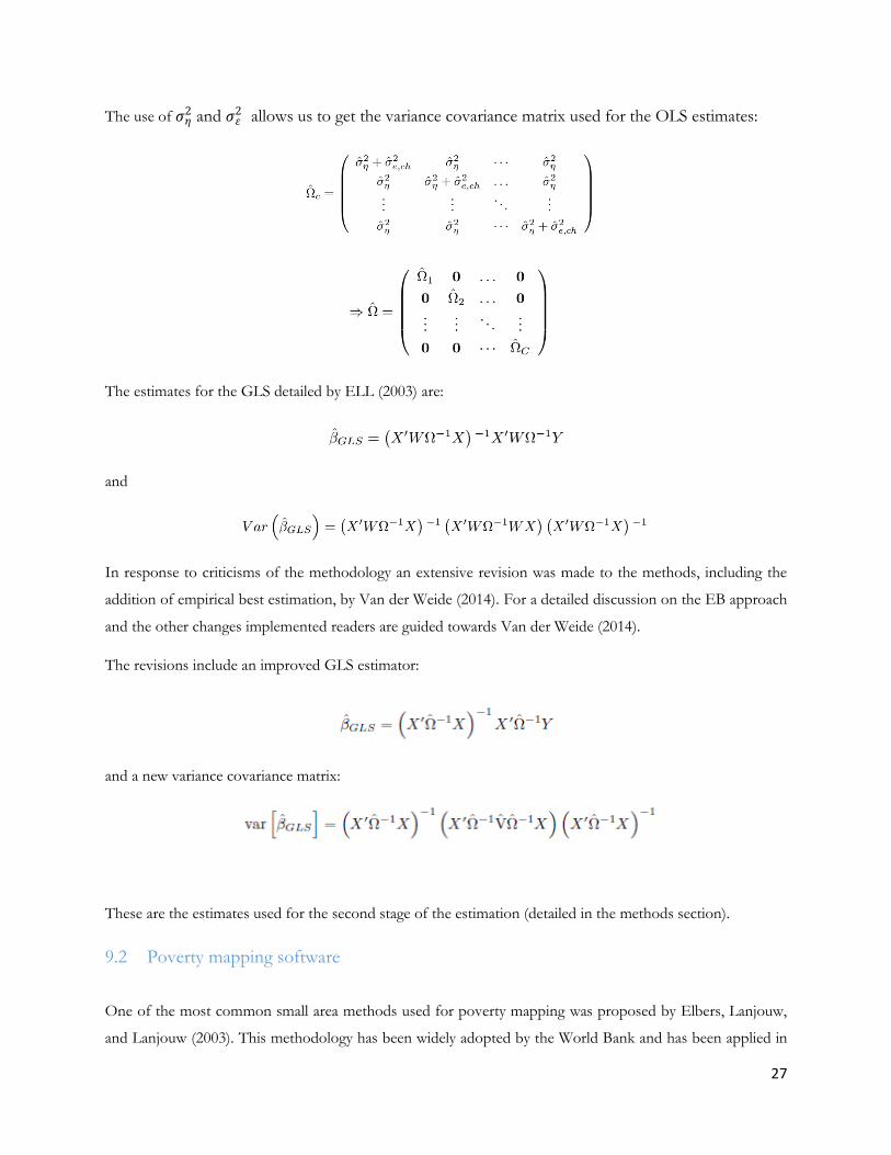
The use of 𝜎𝜂2 and 𝜎𝜀

2 allows us to get the variance covariance matrix used for the OLS estimates:

The estimates for the GLS detailed by ELL (2003) are:

and

In response to criticisms of the methodology an extensive revision was made to the methods, including the

addition of empirical best estimation, by Van der Weide (2014). For a detailed discussion on the EB approach

and the other changes implemented readers are guided towards Van der Weide (2014).

The revisions include an improved GLS estimator:

and a new variance covariance matrix:

These are the estimates used for the second stage of the estimation (detailed in the methods section).

9.2 Poverty mapping software

One of the most common small area methods used for poverty mapping was proposed by Elbers, Lanjouw,

and Lanjouw (2003). This methodology has been widely adopted by the World Bank and has been applied in

28

numerous poverty maps conducted by the institution. In its efforts to make the implementation of the ELL

methodology as simple as possible, the World Bank created a software package that could be easily used by

anyone. The software, PovMap (Zhao, 2006), has proven to be an invaluable resource for the World Bank as

well as for many statistical agencies seeking to create their own poverty maps. The software is freely available

and has a graphical user interface which simplifies its use.

Poverty map results produced in this document have all made use of the PovMap software. The PovMap

software can be downloaded, free of charge, at http://iresearch.worldbank.org/PovMap/PovMap2/.

9.3 Additional tables and graphs

Table 1A: Population weighted candidate variable means in Census and HBS at the Statistical Area

levels

Northwest Central & Eastern Adriatic

Variable name Census HBS-2011 Census HBS-2011 Census HBS-2011

Male 0.4777 0.4730 0.4843 0.4698 0.4873 0.4552

Age [0,5) 0.0515 0.0384 0.0476 0.0367 0.0483 0.0321

Age [5,15) 0.1021 0.0811 0.1082 0.1023 0.0992 0.0971

Age [15,30) 0.1872 0.2079 0.1897 0.1804 0.1817 0.1770

Age [30,65) 0.4937 0.4772 0.4764 0.4852 0.4899 0.4794

Age [65+) 0.1655 0.1954 0.1782 0.1953 0.1810 0.2143

Household size (Share of individuals living in household type) Households size of 1 0.086 0.076 0.086 0.083 0.088 0.094

Households size of 2 0.175 0.198 0.181 0.234 0.195 0.239

Households size of 3 0.200 0.196 0.189 0.154 0.215 0.185

Households size of 4 0.243 0.227 0.237 0.226 0.260 0.217

Households size of 5 0.144 0.177 0.154 0.153 0.133 0.133

Households size of 6 0.083 0.070 0.085 0.091 0.061 0.074

Household size of 7 or more 0.070 0.056 0.067 0.057 0.047 0.059

Occupation (15+) (Share of individuals in households with at least one member) Manager 0.066 0.036 0.031 0.028 0.052 0.038

Professionals 0.188 0.134 0.107 0.063 0.145 0.124

Technicians 0.214 0.161 0.140 0.090 0.183 0.150

Clerical support 0.150 0.170 0.103 0.082 0.127 0.125

Service and sales 0.220 0.196 0.192 0.139 0.254 0.240

29

Skilled agriculture 0.035 0.085 0.064 0.138 0.025 0.042

Craft and trade 0.169 0.198 0.145 0.136 0.140 0.166

Machine operators 0.122 0.121 0.118 0.103 0.093 0.074

Elementary occs. 0.090 0.074 0.103 0.088 0.081 0.073

Labor status, age 15-64 (Share of individuals in households with at least one member) Employed 0.793 0.759 0.689 0.629 0.732 0.714

Retired 0.497 0.554 0.515 0.548 0.492 0.520

Student 0.223 0.270 0.220 0.236 0.221 0.240

Disabled 0.036 0.031 0.052 0.035 0.030 0.031

Other 0.727 0.755 0.794 0.782 0.745 0.752

Industry, age 15-64 (Share of individuals in households with at least one member) Agriculture, mining, and fishing 0.052 0.123 0.112 0.185 0.041 0.067

Manufacturing 0.225 0.207 0.191 0.156 0.147 0.104

Services and Sales 0.684 0.656 0.532 0.447 0.655 0.652

Share of members with education in HH (age 15-64) Primary education 0.075 0.065 0.107 0.123 0.081 0.094

Lower secondary 0.184 0.235 0.263 0.298 0.162 0.165

Upper secondary 0.536 0.559 0.521 0.516 0.578 0.591

Tertiary education 0.206 0.141 0.110 0.063 0.179 0.149

Dwelling characteristics Square meters 90.711 92.227 92.523 96.095 83.187 86.506

Table A2: Alpha model

Coeff. Std Err.

HH dependency ratio -0.2946722 0.18568

Age of oldest member 0.0104073** 0.004439

Constant -4.937768*** 0.24085

Adj. R2 0.0019 Observations 2,229

30

Figure A1: Municipal, City, and districts of Zagreb poverty estimates and 95% confidence intervals

0.2

.4.6

.81

Hea

d c

ou

nt p

ove

rty %

Municipalities, Cities, and Districts of Zagreb

Head count poverty 95% CI

31

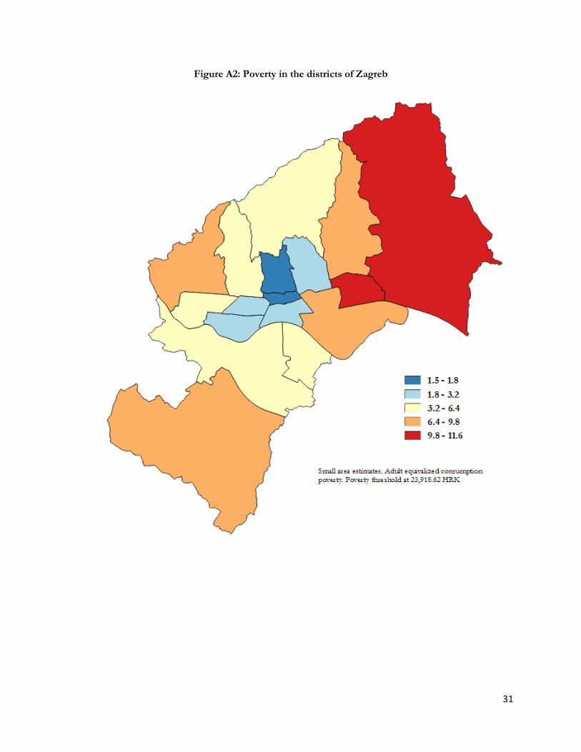
Figure A2: Poverty in the districts of Zagreb

32

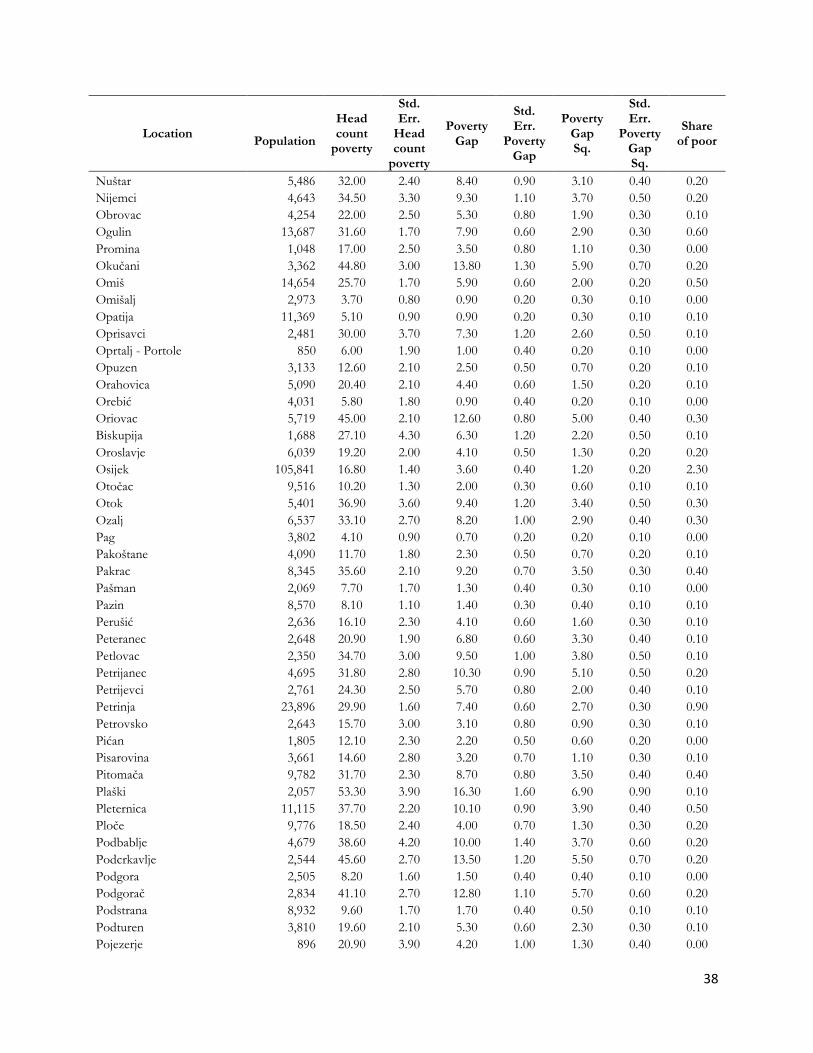
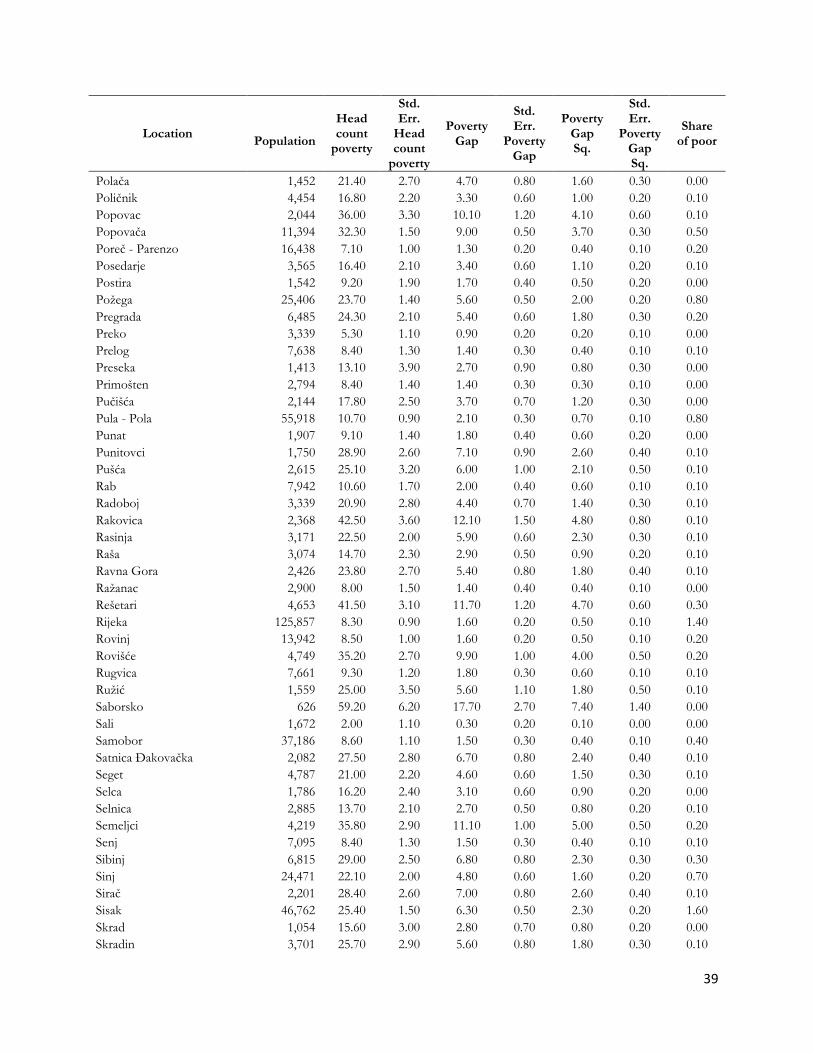
Table 3A: Poverty indicators by LAU-2

Location

Population

Head count

poverty

Std. Err.

Head count

poverty

Poverty Gap

Std. Err.

Poverty Gap

Poverty Gap Sq.

Std. Err.

Poverty Gap Sq.

Share of poor

Donji Grad 35,609 1.50 0.50 0.20 0.10 0.10 0.00 0.10

Gornji Grad-Medvešèak 29,750 1.80 0.40 0.30 0.10 0.10 0.00 0.10

Trnje 41,021 3.00 0.70 0.60 0.10 0.20 0.00 0.20

Maksimir 47,362 3.20 0.80 0.50 0.10 0.10 0.00 0.20

Pešæenica-Žitnjak 55,057 8.50 1.70 1.90 0.40 0.70 0.20 0.60

Novi Zagreb-istok 58,052 4.50 1.00 0.80 0.20 0.20 0.10 0.30

Novi Zagreb-zapad 56,647 4.80 1.10 0.80 0.20 0.20 0.10 0.40

Trešnjevka-sjever 54,197 3.20 0.80 0.60 0.20 0.20 0.10 0.20

Trešnjevka-jug 65,555 2.80 0.70 0.40 0.10 0.10 0.00 0.20

Èrnomerec 37,577 4.70 0.90 0.80 0.20 0.20 0.10 0.20

Gornja Dubrava 60,882 9.20 1.20 1.80 0.30 0.60 0.10 0.70

Donja Dubrava 35,871 11.60 1.80 2.40 0.50 0.80 0.20 0.50

Stenjevec 50,678 5.10 0.90 0.80 0.20 0.20 0.10 0.30

Podsused-Vrapèe 44,580 9.20 1.40 1.70 0.30 0.50 0.10 0.50

Podsljeme 18,858 6.40 1.50 1.10 0.30 0.30 0.10 0.20

Sesvete 68,924 11.00 1.60 2.10 0.40 0.60 0.10 1.00

Brezovica 11,720 9.80 1.90 1.80 0.40 0.50 0.20 0.20

Grad Zagreb 772,340 5.90 0.90 1.10 0.20 0.30 0.10 6.00

Andrijaševci 4,020 41.30 2.50 11.20 0.90 4.20 0.50 0.20

Antunovac 3,610 39.30 3.70 10.60 1.40 4.10 0.70 0.20

Babina Greda 3,516 27.70 3.00 6.70 1.00 2.40 0.40 0.10

Bakar 8,211 10.90 1.40 2.10 0.30 0.60 0.10 0.10

Bale - Valle 1,125 7.20 1.70 1.30 0.40 0.40 0.10 0.00

Barban 2,688 10.40 1.90 1.80 0.40 0.50 0.10 0.00

Barilović 2,967 41.40 2.70 10.80 1.10 4.00 0.50 0.20

Baška 1,658 13.50 2.10 2.80 0.50 0.90 0.20 0.00

Baška Voda 2,773 11.10 1.70 2.00 0.40 0.60 0.10 0.00

Bebrina 3,185 41.70 2.40 11.80 1.00 4.60 0.50 0.20

Bedekovčina 7,759 17.60 1.80 3.90 0.50 1.30 0.20 0.20

Bednja 3,954 40.00 4.50 10.80 1.70 4.10 0.80 0.20

Beli Manastir 9,459 30.30 1.90 8.40 0.70 3.50 0.30 0.40

Belica 3,150 12.40 1.90 2.40 0.50 0.70 0.20 0.10

Belišće 10,509 32.20 1.90 9.10 0.70 3.90 0.30 0.40

Benkovac 10,934 24.20 2.10 5.60 0.60 1.90 0.30 0.30

Berek 1,437 48.20 3.80 15.90 1.60 7.40 0.90 0.10

Beretinec 2,117 28.10 3.70 6.30 1.10 2.10 0.40 0.10

Bibinje 3,969 14.60 2.40 2.80 0.60 0.80 0.20 0.10

Bilje 5,590 25.10 2.80 6.00 0.90 2.10 0.40 0.20

Biograd Na Moru 5,501 12.60 1.60 2.40 0.40 0.70 0.20 0.10

Bizovac 4,456 28.60 2.30 6.70 0.80 2.30 0.30 0.20

Bjelovar 39,061 24.70 1.80 6.10 0.60 2.30 0.30 1.30

Blato 3,460 6.90 2.10 1.20 0.40 0.30 0.10 0.00

Bogdanovci 1,877 36.30 3.30 9.40 1.20 3.50 0.60 0.10

Bol 1,576 4.10 1.00 0.70 0.20 0.20 0.10 0.00

33

Location

Population

Head count

poverty

Std. Err.

Head count

poverty

Poverty Gap

Std. Err.

Poverty Gap

Poverty Gap Sq.

Std. Err.

Poverty Gap Sq.

Share of poor

Borovo 4,857 50.70 3.80 15.30 1.70 6.40 0.90 0.30

Bosiljevo 1,253 44.10 3.70 11.70 1.40 4.40 0.70 0.10

Bošnjaci 3,748 29.00 2.00 7.50 0.70 2.80 0.30 0.10

Brckovljani 6,432 13.70 1.50 3.00 0.40 1.00 0.20 0.10

Brdovec 11,048 8.90 1.20 1.60 0.30 0.50 0.10 0.10

Brestovac 3,691 44.20 2.20 12.60 0.90 5.00 0.40 0.20

Breznica 2,188 36.10 4.50 9.00 1.60 3.20 0.70 0.10

Brinje 3,180 25.00 2.70 6.10 0.80 2.20 0.40 0.10

Brod Moravice 849 20.60 2.70 6.90 0.80 3.50 0.40 0.00

Brodski Stupnik 2,950 38.80 2.30 10.30 0.80 3.90 0.40 0.20

Brtonigla - Verteneglio 1,622 1.70 0.90 0.20 0.10 0.00 0.00 0.00

Budinščina 2,390 25.90 3.40 6.40 1.00 2.30 0.50 0.10

Buje - Buie 5,102 8.90 1.20 1.70 0.30 0.50 0.10 0.10

Buzet 6,048 11.70 1.40 2.20 0.40 0.60 0.10 0.10

Cerna 4,489 30.10 2.00 7.50 0.70 2.70 0.30 0.20

Cernik 3,562 37.30 3.10 10.20 1.10 4.00 0.50 0.20

Cerovlje 1,650 11.10 2.10 2.00 0.50 0.60 0.20 0.00

Cestica 5,504 33.50 3.30 9.00 1.10 3.60 0.50 0.20

Cetingrad 1,921 39.60 3.00 11.00 1.20 4.40 0.60 0.10

Cista Provo 2,310 25.50 3.10 5.80 0.90 2.00 0.40 0.10

Civljane 226 65.80 16.00 20.50 8.10 8.50 4.30 0.00

Cres 2,777 5.40 1.30 0.80 0.30 0.20 0.10 0.00

Crikvenica 10,947 9.80 1.20 1.90 0.30 0.50 0.10 0.10

Crnac 1,445 37.20 3.60 10.10 1.20 4.00 0.60 0.10

Čabar 3,748 23.70 3.20 5.20 0.90 1.70 0.40 0.10

Čačinci 2,758 28.80 2.20 6.80 0.70 2.40 0.30 0.10

Čađavica 1,983 40.50 4.40 10.60 1.60 4.00 0.70 0.10

Čaglin 2,363 47.70 3.40 14.20 1.50 5.90 0.80 0.10

Čakovec 26,422 11.40 1.00 3.30 0.30 1.50 0.20 0.40

Čavle 7,071 10.60 1.20 2.00 0.30 0.60 0.10 0.10

Čazma 7,926 32.40 3.10 8.30 1.10 3.10 0.50 0.30

Čeminac 2,780 34.10 3.20 8.70 1.10 3.30 0.50 0.10

Čepin 11,299 22.50 1.80 5.20 0.60 1.80 0.20 0.30

Darda 6,746 34.60 1.70 10.60 0.70 4.70 0.40 0.30

Daruvar 11,482 25.20 1.80 5.70 0.60 1.90 0.20 0.40

Davor 2,967 34.00 3.10 8.80 1.00 3.30 0.50 0.10

Delnice 5,747 14.90 1.90 3.70 0.50 1.50 0.20 0.10

Desinić 2,604 22.20 2.70 4.80 0.80 1.50 0.30 0.10

Dežanovac 2,706 37.10 3.20 10.00 1.20 3.90 0.60 0.10

Dicmo 2,753 47.70 3.80 13.70 1.60 5.40 0.80 0.20

Dobrinj 2,051 7.70 1.40 1.60 0.30 0.50 0.10 0.00

Domašinec 2,217 17.30 2.40 4.40 0.50 1.80 0.30 0.10

Brela 1,698 4.90 1.80 0.80 0.30 0.20 0.10 0.00

Donja Dubrava 1,895 11.90 2.20 2.20 0.50 0.70 0.20 0.00

Donja Stubica 5,375 19.50 1.80 4.20 0.50 1.40 0.20 0.10

Donja Voća 2,392 32.10 4.10 7.90 1.30 2.80 0.60 0.10

34

Location

Population

Head count

poverty

Std. Err.

Head count

poverty

Poverty Gap

Std. Err.

Poverty Gap

Poverty Gap Sq.

Std. Err.

Poverty Gap Sq.

Share of poor

Donji Andrijevci 3,666 35.00 2.10 9.50 0.80 3.60 0.40 0.20

Donji Kraljevec 4,527 11.40 1.80 2.00 0.40 0.60 0.10 0.10

Donji Kukuruzari 1,634 48.10 3.00 14.80 1.30 6.30 0.70 0.10

Donji Lapac 2,028 15.90 2.30 3.40 0.60 1.10 0.20 0.00

Martijanec 3,788 38.30 3.60 9.50 1.30 3.40 0.60 0.20

Donji Miholjac 9,275 18.70 1.90 4.30 0.60 1.50 0.20 0.20

Muć 3,838 31.70 2.40 7.40 0.70 2.50 0.30 0.20

Proložac 3,491 32.60 3.30 8.10 1.10 2.90 0.50 0.10

Donji Vidovec 1,378 17.50 3.10 4.30 0.70 1.70 0.30 0.00

Draganić 2,665 44.00 2.90 12.80 1.10 5.40 0.60 0.20

Draž 2,681 26.50 3.00 6.70 0.90 2.50 0.40 0.10

Drenovci 4,969 30.60 2.00 7.90 0.80 3.00 0.40 0.20

Drenje 2,592 48.00 3.90 14.40 1.70 6.10 0.90 0.20

Drniš 7,422 19.00 1.70 4.10 0.50 1.30 0.20 0.20

Drnje 1,832 18.80 2.70 5.60 0.80 2.60 0.40 0.00

Dubrava 5,023 19.60 2.70 4.20 0.80 1.40 0.30 0.10

Dubrovnik 41,417 8.60 1.00 1.60 0.30 0.40 0.10 0.50

Duga Resa 11,120 34.30 1.90 8.70 0.70 3.20 0.30 0.50

Dugi Rat 6,982 16.50 1.80 3.30 0.50 1.00 0.20 0.20

Dugo Selo 17,201 10.60 1.60 2.00 0.40 0.60 0.10 0.20

Dvor 5,478 45.30 3.00 13.00 1.20 5.20 0.60 0.30

Đakovo 26,790 22.50 1.50 5.20 0.50 1.80 0.20 0.80

Đelekovec 1,490 11.80 2.00 2.50 0.50 0.80 0.20 0.00

Đulovac 3,171 45.30 4.70 14.20 2.00 6.10 1.10 0.20

Đurđenovac 6,598 47.70 3.00 14.30 1.30 6.00 0.70 0.40

Đurđevac 8,090 18.40 1.40 5.20 0.40 2.20 0.20 0.20

Đurmanec 4,150 20.90 2.40 4.50 0.70 1.40 0.30 0.10

Erdut 7,108 39.50 2.80 11.00 1.10 4.40 0.50 0.40

Ernestinovo 2,064 38.50 3.70 10.70 1.30 4.30 0.60 0.10

Ervenik 1,098 18.40 3.70 3.80 0.90 1.30 0.40 0.00

Farkaševac 1,889 24.30 3.00 6.00 1.00 2.20 0.50 0.10

Ferdinandovac 1,739 14.80 2.90 3.10 0.70 1.00 0.30 0.00

Feričanci 2,093 31.30 2.70 8.10 0.90 3.10 0.40 0.10

Fužine 1,570 14.80 2.30 3.00 0.60 1.00 0.20 0.00

Garčin 4,729 36.70 3.40 9.80 1.20 3.80 0.60 0.20

Garešnica 10,258 39.50 2.60 11.60 1.10 4.80 0.50 0.50

Generalski Stol 2,586 28.30 3.60 6.70 1.20 2.40 0.50 0.10

Glina 8,757 44.80 2.60 12.90 1.00 5.30 0.50 0.50

Gola 2,389 19.60 2.30 4.50 0.70 1.50 0.30 0.10

Goričan 2,777 8.80 1.60 1.70 0.30 0.50 0.10 0.00

Gorjani 1,564 35.00 3.40 8.80 1.20 3.20 0.50 0.10

Gornja Stubica 5,258 15.30 2.00 2.90 0.50 0.90 0.20 0.10

Gornji Bogićevci 1,957 43.90 3.30 13.40 1.30 5.70 0.70 0.10

Gornji Kneginec 5,252 26.20 2.30 6.10 0.70 2.10 0.30 0.20

Gospić 12,320 11.90 1.40 2.50 0.40 0.80 0.10 0.20

Gračac 4,661 22.40 1.90 5.30 0.60 1.80 0.30 0.10

35

Location

Population

Head count

poverty

Std. Err.

Head count

poverty

Poverty Gap

Std. Err.

Poverty Gap

Poverty Gap Sq.

Std. Err.

Poverty Gap Sq.

Share of poor

Gračišće 1,416 9.50 2.10 1.60 0.40 0.40 0.20 0.00

Gradac 3,237 18.70 1.90 4.40 0.60 1.60 0.30 0.10

Gradec 3,601 14.70 1.70 3.20 0.50 1.00 0.20 0.10

Gradina 3,799 52.30 3.30 16.10 1.50 6.80 0.80 0.30

Gradište 2,627 38.60 2.80 10.90 1.10 4.40 0.50 0.10

Grožnjan - Grisignana 733 8.60 2.10 1.50 0.50 0.40 0.20 0.00

Grubišno Polje 6,383 33.20 2.90 8.90 1.00 3.50 0.50 0.30

Gundinci 2,013 40.50 3.80 10.80 1.40 4.00 0.60 0.10

Gunja 3,637 38.00 2.30 10.70 0.90 4.30 0.50 0.20

Hercegovac 2,378 30.70 3.50 7.70 1.20 2.80 0.50 0.10

Hlebine 1,271 17.30 2.50 4.20 0.70 1.50 0.30 0.00

Hrašćina 1,535 29.00 3.50 6.70 1.00 2.30 0.40 0.10

Hrvace 3,595 35.50 2.60 8.70 0.90 3.10 0.40 0.20

Hrvatska Dubica 2,070 46.30 2.90 14.00 1.30 5.90 0.70 0.10

Hrvatska Kostajnica 2,734 37.80 2.00 10.00 0.70 3.80 0.40 0.10

Breznički Hum 1,314 39.20 4.90 10.00 1.70 3.60 0.80 0.10

Hum Na Sutli 4,851 17.00 2.20 3.50 0.60 1.10 0.20 0.10

Hvar 4,218 7.00 1.10 1.20 0.30 0.30 0.10 0.00

Ilok 6,500 31.80 2.80 8.00 0.90 2.90 0.40 0.30

Imotski 10,671 37.30 3.40 9.60 1.30 3.50 0.60 0.50

Ivanec 13,447 27.30 2.70 6.30 0.90 2.10 0.40 0.50

Ivanić-Grad 14,292 10.40 1.10 2.30 0.30 0.80 0.10 0.20

Ivankovo 7,762 31.20 2.60 7.70 0.90 2.70 0.40 0.30

Ivanska 2,908 39.60 5.00 11.10 1.90 4.50 0.90 0.20

Jakovlje 3,813 16.30 2.10 3.20 0.50 0.90 0.20 0.10

Jakšić 3,986 24.50 2.20 5.60 0.70 1.90 0.30 0.10

Jalžabet 3,120 35.80 3.20 9.10 1.10 3.40 0.50 0.10

Jarmina 2,440 29.30 3.20 7.00 1.00 2.40 0.40 0.10

Jasenice 1,395 16.40 2.70 2.90 0.60 0.80 0.20 0.00

Jasenovac 1,987 39.50 2.70 11.40 1.10 4.80 0.60 0.10

Jastrebarsko 15,625 8.60 1.20 1.60 0.30 0.50 0.10 0.20

Jelenje 5,277 10.30 1.60 1.80 0.30 0.50 0.10 0.10

Jelsa 3,556 10.20 1.50 1.90 0.40 0.60 0.10 0.00

Josipdol 3,723 43.60 2.00 12.70 0.80 5.30 0.40 0.20

Kali 1,628 5.30 1.50 0.80 0.30 0.20 0.10 0.00

Kanfanar 1,541 8.80 1.80 1.40 0.40 0.40 0.10 0.00

Kapela 2,939 44.50 3.00 12.70 1.20 5.20 0.60 0.20

Kaptol 3,446 33.80 2.20 8.70 0.80 3.30 0.40 0.20

Karlobag 915 11.40 2.40 2.30 0.50 0.70 0.20 0.00

Karlovac 54,120 26.40 1.60 6.30 0.50 2.20 0.20 1.90

Kastav 10,346 7.40 1.30 1.20 0.30 0.30 0.10 0.10

Kaštela 38,044 12.90 1.20 2.40 0.30 0.70 0.10 0.60

Kijevo 415 21.30 3.20 4.60 1.00 1.50 0.40 0.00

Kistanje 3,429 41.00 4.40 13.20 1.80 5.80 1.00 0.20

Klakar 2,251 26.50 3.10 6.10 1.00 2.10 0.40 0.10

Klana 1,966 18.80 2.90 3.60 0.80 1.00 0.30 0.00

36

Location

Population

Head count

poverty

Std. Err.

Head count

poverty

Poverty Gap

Std. Err.

Poverty Gap

Poverty Gap Sq.

Std. Err.

Poverty Gap Sq.

Share of poor

Klanjec 2,911 12.30 2.10 2.40 0.50 0.80 0.20 0.00

Klenovnik 2,006 26.50 3.60 6.00 1.10 2.00 0.40 0.10

Klinča Sela 5,108 11.20 2.00 2.00 0.50 0.50 0.20 0.10

Klis 4,738 16.10 1.60 3.10 0.40 0.90 0.20 0.10

Kloštar Ivanić 5,990 14.70 2.00 3.20 0.60 1.10 0.20 0.10

Kloštar Podravski 3,200 28.00 2.40 8.70 0.90 4.00 0.50 0.10

Kneževi Vinogradi 4,517 25.70 1.90 6.80 0.60 2.60 0.30 0.20

Knin 15,011 17.20 1.90 3.60 0.50 1.20 0.20 0.30

Komiža 1,519 15.70 2.20 3.30 0.50 1.10 0.20 0.00

Konavle 8,549 8.60 2.00 1.40 0.40 0.40 0.10 0.10

Končanica 2,340 24.30 4.20 6.20 1.20 2.30 0.50 0.10

Konjščina 3,658 15.30 2.30 3.20 0.60 1.00 0.20 0.10

Koprivnica 29,930 9.60 0.90 2.00 0.20 0.70 0.10 0.40

Koprivnički Bregi 2,270 16.50 2.50 3.60 0.70 1.20 0.30 0.00

Koprivnički Ivanec 1,972 9.50 1.60 1.90 0.40 0.70 0.20 0.00

Korčula 5,585 4.70 1.10 0.70 0.20 0.20 0.10 0.00

Koška 3,889 26.30 2.50 6.80 0.90 2.60 0.40 0.10

Kotoriba 3,080 24.00 2.00 8.40 0.70 4.20 0.40 0.10

Kraljevec Na Sutli 1,727 13.50 3.20 2.60 0.80 0.80 0.30 0.00

Kraljevica 4,490 9.60 1.60 1.70 0.40 0.50 0.10 0.10

Krapina 12,105 15.50 1.50 3.10 0.40 1.00 0.20 0.20

Krapinske Toplice 5,249 12.30 1.90 2.40 0.50 0.70 0.20 0.10

Križ 6,794 16.50 1.60 3.60 0.50 1.20 0.20 0.10

Križevci 20,631 12.90 1.10 2.60 0.30 0.80 0.10 0.30

Krk 5,951 5.10 1.10 0.80 0.20 0.20 0.10 0.00

Krnjak 1,826 60.90 3.20 19.60 1.60 8.70 0.90 0.10

Kršan 2,913 9.80 1.60 1.70 0.40 0.50 0.10 0.00

Kula Norinska 1,608 14.70 2.20 3.00 0.50 0.90 0.20 0.00

Kutina 22,337 25.00 1.80 6.40 0.60 2.50 0.30 0.70

Kutjevo 6,165 42.20 2.00 12.00 0.80 4.90 0.40 0.30

Labin 11,497 12.60 1.40 2.40 0.40 0.70 0.10 0.20

Lanišće 328 6.30 2.80 1.00 0.50 0.30 0.20 0.00

Lasinja 1,612 41.70 3.60 11.40 1.40 4.40 0.70 0.10

Lastovo 792 4.60 1.90 0.80 0.40 0.20 0.10 0.00

Legrad 2,185 8.70 2.80 2.20 0.70 0.90 0.30 0.00

Lekenik 5,885 27.10 3.30 6.50 1.00 2.30 0.50 0.20

Lepoglava 7,437 28.70 3.20 6.90 1.00 2.40 0.40 0.30

Levanjska Varoš 1,016 70.50 4.30 26.60 2.60 13.20 1.70 0.10

Lipik 6,002 30.80 2.30 8.10 0.70 3.10 0.30 0.20

Lipovljani 3,450 25.60 3.00 6.00 1.00 2.10 0.40 0.10

Lišane Ostrovičke 686 12.30 3.60 2.20 0.80 0.60 0.30 0.00

Ližnjan - Lisignano 3,806 11.00 1.70 2.10 0.40 0.60 0.10 0.10

Lobor 2,818 14.40 2.20 2.80 0.60 0.80 0.20 0.10

Lokve 1,004 27.70 4.30 6.00 1.20 1.90 0.50 0.00

Lovas 1,207 29.30 3.40 7.20 1.00 2.60 0.50 0.00

Lovinac 995 13.50 2.60 3.30 0.80 1.10 0.40 0.00

37

Location

Population

Head count

poverty

Std. Err.

Head count

poverty

Poverty Gap

Std. Err.

Poverty Gap

Poverty Gap Sq.

Std. Err.

Poverty Gap Sq.

Share of poor

Lovran 4,033 4.70 0.90 0.80 0.20 0.20 0.10 0.00

Lovreć 1,691 20.20 2.50 4.30 0.70 1.40 0.30 0.00

Ludbreg 8,223 21.90 2.00 5.00 0.60 1.70 0.30 0.20

Lukač 3,568 36.50 2.60 9.90 1.00 3.90 0.50 0.20

Lupoglav 918 9.10 2.00 1.70 0.50 0.50 0.20 0.00

Ljubešćica 1,837 27.60 3.80 6.30 1.00 2.10 0.40 0.10

Mače 2,511 15.80 2.30 3.20 0.60 1.00 0.20 0.10

Makarska 13,684 10.80 1.20 2.00 0.30 0.60 0.10 0.20

Mala Subotica 5,274 22.50 1.70 8.50 0.60 4.60 0.40 0.20

Mali Bukovec 2,185 35.80 2.80 9.30 1.00 3.50 0.50 0.10

Mali Lošinj 7,916 5.50 0.90 0.90 0.20 0.30 0.10 0.10

Malinska-Dubašnica 3,050 9.20 1.50 1.70 0.40 0.50 0.10 0.00

Marčana 4,199 15.30 2.10 3.00 0.50 0.90 0.20 0.10

Marija Bistrica 5,889 12.60 1.70 2.40 0.40 0.70 0.20 0.10

Marijanci 2,358 23.90 2.90 5.80 0.90 2.10 0.40 0.10

Marina 4,496 30.30 2.70 7.10 0.90 2.40 0.40 0.20

Martinska Ves 3,393 37.20 3.00 9.80 1.10 3.70 0.50 0.20

Maruševec 6,275 32.20 2.90 7.50 1.00 2.50 0.40 0.30

Matulji 11,121 6.50 1.10 1.10 0.20 0.30 0.10 0.10

Medulin 6,374 8.60 1.30 1.70 0.30 0.60 0.10 0.10

Metković 15,956 17.80 2.00 3.70 0.50 1.20 0.20 0.40

Mihovljan 1,921 37.90 4.10 9.50 1.40 3.40 0.60 0.10

Mikleuš 1,449 38.30 2.80 10.80 1.10 4.30 0.60 0.10

Milna 1,022 13.90 2.50 2.70 0.70 0.80 0.30 0.00

Mljet 1,061 3.80 1.30 0.70 0.30 0.20 0.10 0.00

Molve 2,147 22.10 3.30 5.10 1.00 1.70 0.40 0.10

Podravska Moslavina 1,153 23.60 3.50 5.70 1.00 2.10 0.50 0.00

Mošćenička Draga 1,526 7.10 1.90 1.10 0.40 0.30 0.10 0.00

Motovun - Montona 916 14.30 3.10 3.00 0.70 1.00 0.30 0.00

Mrkopalj 1,205 20.80 3.60 4.00 0.80 1.20 0.30 0.00

Mursko-Središće 6,209 16.60 1.70 4.40 0.50 1.80 0.20 0.10

Našice 15,912 21.10 1.80 5.20 0.50 2.00 0.20 0.40

Nedelišće 11,700 18.70 1.30 6.80 0.50 3.50 0.30 0.30

Nerežišća 845 4.40 1.80 0.70 0.30 0.20 0.10 0.00

Netretić 2,791 57.80 3.50 17.10 1.60 7.00 0.80 0.20

Nin 2,710 10.00 2.10 1.70 0.50 0.50 0.20 0.00

Nova Bukovica 1,769 47.30 3.30 13.20 1.30 5.20 0.60 0.10

Nova Gradiška 13,880 32.00 1.90 8.50 0.70 3.30 0.30 0.60

Nova Kapela 4,108 37.10 3.10 9.80 1.20 3.70 0.60 0.20

Nova Rača 3,391 32.20 3.50 8.10 1.20 2.90 0.50 0.10

Novalja 3,613 4.30 1.00 0.70 0.20 0.20 0.10 0.00

Novi Marof 13,103 22.30 2.30 4.80 0.70 1.60 0.30 0.40

Novi Vinodolski 4,976 7.50 1.10 1.50 0.30 0.50 0.10 0.00

Novigrad - Cittanova 4,145 8.00 1.20 1.40 0.30 0.40 0.10 0.00

Novigrad Podravski 2,758 16.30 1.80 4.20 0.50 1.70 0.30 0.10

Novska 13,404 30.20 1.80 7.90 0.70 3.00 0.30 0.50

38

Location

Population

Head count

poverty

Std. Err.

Head count

poverty

Poverty Gap

Std. Err.

Poverty Gap

Poverty Gap Sq.

Std. Err.

Poverty Gap Sq.

Share of poor

Nuštar 5,486 32.00 2.40 8.40 0.90 3.10 0.40 0.20

Nijemci 4,643 34.50 3.30 9.30 1.10 3.70 0.50 0.20

Obrovac 4,254 22.00 2.50 5.30 0.80 1.90 0.30 0.10

Ogulin 13,687 31.60 1.70 7.90 0.60 2.90 0.30 0.60

Promina 1,048 17.00 2.50 3.50 0.80 1.10 0.30 0.00

Okučani 3,362 44.80 3.00 13.80 1.30 5.90 0.70 0.20

Omiš 14,654 25.70 1.70 5.90 0.60 2.00 0.20 0.50

Omišalj 2,973 3.70 0.80 0.90 0.20 0.30 0.10 0.00

Opatija 11,369 5.10 0.90 0.90 0.20 0.30 0.10 0.10

Oprisavci 2,481 30.00 3.70 7.30 1.20 2.60 0.50 0.10

Oprtalj - Portole 850 6.00 1.90 1.00 0.40 0.20 0.10 0.00

Opuzen 3,133 12.60 2.10 2.50 0.50 0.70 0.20 0.10

Orahovica 5,090 20.40 2.10 4.40 0.60 1.50 0.20 0.10

Orebić 4,031 5.80 1.80 0.90 0.40 0.20 0.10 0.00

Oriovac 5,719 45.00 2.10 12.60 0.80 5.00 0.40 0.30

Biskupija 1,688 27.10 4.30 6.30 1.20 2.20 0.50 0.10

Oroslavje 6,039 19.20 2.00 4.10 0.50 1.30 0.20 0.20

Osijek 105,841 16.80 1.40 3.60 0.40 1.20 0.20 2.30

Otočac 9,516 10.20 1.30 2.00 0.30 0.60 0.10 0.10

Otok 5,401 36.90 3.60 9.40 1.20 3.40 0.50 0.30

Ozalj 6,537 33.10 2.70 8.20 1.00 2.90 0.40 0.30

Pag 3,802 4.10 0.90 0.70 0.20 0.20 0.10 0.00

Pakoštane 4,090 11.70 1.80 2.30 0.50 0.70 0.20 0.10

Pakrac 8,345 35.60 2.10 9.20 0.70 3.50 0.30 0.40

Pašman 2,069 7.70 1.70 1.30 0.40 0.30 0.10 0.00

Pazin 8,570 8.10 1.10 1.40 0.30 0.40 0.10 0.10

Perušić 2,636 16.10 2.30 4.10 0.60 1.60 0.30 0.10

Peteranec 2,648 20.90 1.90 6.80 0.60 3.30 0.40 0.10

Petlovac 2,350 34.70 3.00 9.50 1.00 3.80 0.50 0.10

Petrijanec 4,695 31.80 2.80 10.30 0.90 5.10 0.50 0.20

Petrijevci 2,761 24.30 2.50 5.70 0.80 2.00 0.40 0.10

Petrinja 23,896 29.90 1.60 7.40 0.60 2.70 0.30 0.90

Petrovsko 2,643 15.70 3.00 3.10 0.80 0.90 0.30 0.10

Pićan 1,805 12.10 2.30 2.20 0.50 0.60 0.20 0.00

Pisarovina 3,661 14.60 2.80 3.20 0.70 1.10 0.30 0.10

Pitomača 9,782 31.70 2.30 8.70 0.80 3.50 0.40 0.40

Plaški 2,057 53.30 3.90 16.30 1.60 6.90 0.90 0.10

Pleternica 11,115 37.70 2.20 10.10 0.90 3.90 0.40 0.50

Ploče 9,776 18.50 2.40 4.00 0.70 1.30 0.30 0.20

Podbablje 4,679 38.60 4.20 10.00 1.40 3.70 0.60 0.20

Podcrkavlje 2,544 45.60 2.70 13.50 1.20 5.50 0.70 0.20

Podgora 2,505 8.20 1.60 1.50 0.40 0.40 0.10 0.00

Podgorač 2,834 41.10 2.70 12.80 1.10 5.70 0.60 0.20

Podstrana 8,932 9.60 1.70 1.70 0.40 0.50 0.10 0.10

Podturen 3,810 19.60 2.10 5.30 0.60 2.30 0.30 0.10

Pojezerje 896 20.90 3.90 4.20 1.00 1.30 0.40 0.00

39

Location

Population

Head count

poverty

Std. Err.

Head count

poverty

Poverty Gap

Std. Err.

Poverty Gap

Poverty Gap Sq.

Std. Err.

Poverty Gap Sq.

Share of poor

Polača 1,452 21.40 2.70 4.70 0.80 1.60 0.30 0.00

Poličnik 4,454 16.80 2.20 3.30 0.60 1.00 0.20 0.10

Popovac 2,044 36.00 3.30 10.10 1.20 4.10 0.60 0.10

Popovača 11,394 32.30 1.50 9.00 0.50 3.70 0.30 0.50

Poreč - Parenzo 16,438 7.10 1.00 1.30 0.20 0.40 0.10 0.20

Posedarje 3,565 16.40 2.10 3.40 0.60 1.10 0.20 0.10

Postira 1,542 9.20 1.90 1.70 0.40 0.50 0.20 0.00

Požega 25,406 23.70 1.40 5.60 0.50 2.00 0.20 0.80

Pregrada 6,485 24.30 2.10 5.40 0.60 1.80 0.30 0.20

Preko 3,339 5.30 1.10 0.90 0.20 0.20 0.10 0.00

Prelog 7,638 8.40 1.30 1.40 0.30 0.40 0.10 0.10

Preseka 1,413 13.10 3.90 2.70 0.90 0.80 0.30 0.00

Primošten 2,794 8.40 1.40 1.40 0.30 0.30 0.10 0.00

Pučišća 2,144 17.80 2.50 3.70 0.70 1.20 0.30 0.00

Pula - Pola 55,918 10.70 0.90 2.10 0.30 0.70 0.10 0.80

Punat 1,907 9.10 1.40 1.80 0.40 0.60 0.20 0.00

Punitovci 1,750 28.90 2.60 7.10 0.90 2.60 0.40 0.10

Pušća 2,615 25.10 3.20 6.00 1.00 2.10 0.50 0.10

Rab 7,942 10.60 1.70 2.00 0.40 0.60 0.10 0.10

Radoboj 3,339 20.90 2.80 4.40 0.70 1.40 0.30 0.10

Rakovica 2,368 42.50 3.60 12.10 1.50 4.80 0.80 0.10

Rasinja 3,171 22.50 2.00 5.90 0.60 2.30 0.30 0.10

Raša 3,074 14.70 2.30 2.90 0.50 0.90 0.20 0.10

Ravna Gora 2,426 23.80 2.70 5.40 0.80 1.80 0.40 0.10

Ražanac 2,900 8.00 1.50 1.40 0.40 0.40 0.10 0.00

Rešetari 4,653 41.50 3.10 11.70 1.20 4.70 0.60 0.30

Rijeka 125,857 8.30 0.90 1.60 0.20 0.50 0.10 1.40

Rovinj 13,942 8.50 1.00 1.60 0.20 0.50 0.10 0.20

Rovišće 4,749 35.20 2.70 9.90 1.00 4.00 0.50 0.20

Rugvica 7,661 9.30 1.20 1.80 0.30 0.60 0.10 0.10

Ružić 1,559 25.00 3.50 5.60 1.10 1.80 0.50 0.10

Saborsko 626 59.20 6.20 17.70 2.70 7.40 1.40 0.00

Sali 1,672 2.00 1.10 0.30 0.20 0.10 0.00 0.00

Samobor 37,186 8.60 1.10 1.50 0.30 0.40 0.10 0.40

Satnica Đakovačka 2,082 27.50 2.80 6.70 0.80 2.40 0.40 0.10

Seget 4,787 21.00 2.20 4.60 0.60 1.50 0.30 0.10

Selca 1,786 16.20 2.40 3.10 0.60 0.90 0.20 0.00

Selnica 2,885 13.70 2.10 2.70 0.50 0.80 0.20 0.10

Semeljci 4,219 35.80 2.90 11.10 1.00 5.00 0.50 0.20

Senj 7,095 8.40 1.30 1.50 0.30 0.40 0.10 0.10

Sibinj 6,815 29.00 2.50 6.80 0.80 2.30 0.30 0.30

Sinj 24,471 22.10 2.00 4.80 0.60 1.60 0.20 0.70

Sirač 2,201 28.40 2.60 7.00 0.80 2.60 0.40 0.10

Sisak 46,762 25.40 1.50 6.30 0.50 2.30 0.20 1.60

Skrad 1,054 15.60 3.00 2.80 0.70 0.80 0.20 0.00

Skradin 3,701 25.70 2.90 5.60 0.80 1.80 0.30 0.10

40

Location

Population

Head count

poverty

Std. Err.

Head count

poverty

Poverty Gap

Std. Err.

Poverty Gap

Poverty Gap Sq.

Std. Err.

Poverty Gap Sq.

Share of poor

Slatina 13,529 25.80 1.80 6.20 0.60 2.20 0.30 0.50

Slavonski Brod 57,296 28.80 1.40 7.50 0.50 2.90 0.30 2.20

Slavonski Šamac 2,112 44.90 4.10 12.80 1.60 5.20 0.80 0.10

Slivno 1,906 14.70 2.40 3.10 0.60 1.10 0.20 0.00

Slunj 5,012 46.20 3.00 12.70 1.30 4.90 0.70 0.30

Smokvica 874 3.30 1.90 0.50 0.30 0.10 0.10 0.00

Sokolovac 3,346 39.40 4.20 10.60 1.60 4.00 0.80 0.20

Solin 23,670 20.50 2.00 4.30 0.60 1.40 0.20 0.60

Sopje 2,242 40.30 5.50 10.80 2.00 4.20 0.90 0.10

Split 173,163 11.30 0.90 2.10 0.30 0.60 0.10 2.60

Sračinec 4,689 37.60 3.50 9.30 1.20 3.40 0.50 0.20

Stankovci 1,982 29.20 3.30 6.70 0.90 2.30 0.40 0.10

Stara Gradiška 1,349 58.00 3.10 18.00 1.50 7.60 0.90 0.10

Stari Grad 2,744 8.40 1.40 1.50 0.30 0.40 0.10 0.00

Stari Jankovci 4,322 45.60 2.80 13.50 1.10 5.60 0.60 0.30

Stari Mikanovci 2,864 40.50 2.50 11.50 1.00 4.60 0.50 0.20

Starigrad 1,869 8.70 1.80 1.50 0.40 0.40 0.20 0.00

Staro Petrovo Selo 5,090 41.60 3.00 11.80 1.20 4.70 0.60 0.30

Ston 2,287 9.00 1.80 1.70 0.40 0.50 0.10 0.00

Strizivojna 2,494 35.00 2.70 9.10 1.00 3.40 0.50 0.10

Stubičke Toplice 2,736 10.40 1.60 1.90 0.40 0.50 0.10 0.00

Sućuraj 458 10.00 3.10 1.60 0.70 0.40 0.20 0.00

Suhopolje 6,477 36.20 2.20 9.70 0.80 3.80 0.40 0.30

Sukošan 4,533 7.60 1.60 1.30 0.30 0.30 0.10 0.00

Sunja 5,709 43.90 2.50 12.20 1.00 4.90 0.50 0.30

Supetar 3,997 5.80 1.00 0.90 0.20 0.20 0.10 0.00

Sveti Filip I Jakov 4,434 12.00 1.70 2.40 0.40 0.70 0.20 0.10

Sveti Ivan Zelina 15,623 13.30 1.40 2.60 0.40 0.80 0.10 0.30

Sveti Križ Začretje 6,037 19.50 2.30 4.10 0.60 1.30 0.20 0.20

Sveti Lovreč 1,014 11.40 2.30 2.10 0.50 0.60 0.20 0.00

Sveta Nedelja 2,880 10.10 1.40 1.80 0.30 0.50 0.10 0.00

Sveti Petar U Šumi 1,052 8.80 2.20 1.30 0.40 0.30 0.10 0.00

Svetvinčenat 2,184 12.00 2.10 2.10 0.50 0.60 0.20 0.00

Sveta Nedelja 17,785 8.70 1.70 1.50 0.30 0.40 0.10 0.20

Sveti Đurđ 3,763 39.70 3.30 10.60 1.20 4.20 0.60 0.20

Sveti Ilija 3,357 29.70 3.40 6.50 1.00 2.10 0.40 0.10

Sveti Ivan Žabno 5,086 15.80 2.10 3.20 0.50 1.00 0.20 0.10

Sveti Juraj Na Bregu 4,909 9.80 1.60 1.70 0.30 0.50 0.10 0.10

Sveti Martin Na Muri 2,586 16.80 2.10 3.30 0.60 1.00 0.20 0.10

Sveti Petar Orehovec 4,449 34.90 4.90 8.30 1.60 2.90 0.70 0.20

Šestanovac 1,849 18.00 2.40 3.70 0.70 1.10 0.30 0.00

Šibenik 45,426 8.80 1.00 1.60 0.20 0.40 0.10 0.50

Škabrnja 1,770 8.30 2.50 1.30 0.50 0.30 0.20 0.00

Šolta 1,668 11.50 2.10 2.30 0.50 0.70 0.20 0.00

Špišić Bukovica 4,171 46.10 2.90 13.50 1.10 5.50 0.60 0.30

Štefanje 1,988 33.00 3.50 9.80 1.10 4.50 0.60 0.10

41

Location

Population

Head count

poverty

Std. Err.

Head count

poverty

Poverty Gap

Std. Err.

Poverty Gap

Poverty Gap Sq.

Std. Err.

Poverty Gap Sq.

Share of poor

Štrigova 2,526 9.10 1.90 1.70 0.40 0.50 0.10 0.00

Tinjan 1,660 13.00 2.20 2.30 0.50 0.60 0.20 0.00

Tisno 3,089 5.30 1.10 0.80 0.20 0.20 0.10 0.00

Plitvička Jezera 4,299 11.90 1.60 2.40 0.40 0.70 0.10 0.10

Tompojevci 1,523 30.30 3.40 7.10 1.10 2.40 0.50 0.10

Topusko 2,956 39.00 2.60 10.40 0.90 3.90 0.50 0.20

Tordinci 2,004 47.10 3.50 13.20 1.40 5.10 0.70 0.10

Tovarnik 2,736 24.80 2.40 5.80 0.70 2.10 0.30 0.10

Trilj 8,801 34.80 2.50 8.70 0.80 3.10 0.40 0.40

Trnava 1,568 47.70 3.30 14.30 1.40 6.00 0.80 0.10

Trnovec Bartolovečki 6,470 23.60 2.30 4.90 0.60 1.50 0.20 0.20

Trogir 12,784 14.40 1.40 2.80 0.40 0.80 0.10 0.20

Trpinja 5,386 40.50 3.40 10.80 1.30 4.10 0.60 0.30

Tuhelj 1,973 16.50 3.10 3.30 0.80 1.00 0.30 0.00

Udbina 1,791 14.50 2.40 3.30 0.60 1.10 0.30 0.00

Umag 13,383 7.30 1.00 1.30 0.20 0.40 0.10 0.10

Unešić 1,637 20.30 3.60 4.20 0.90 1.30 0.40 0.00

Valpovo 11,216 27.30 1.70 6.60 0.60 2.40 0.30 0.40

Varaždin 45,378 10.10 1.30 1.90 0.30 0.60 0.10 0.60

Varaždinske Toplice 6,316 21.60 2.20 4.60 0.70 1.50 0.30 0.20

Vela Luka 4,059 8.70 1.50 1.60 0.30 0.50 0.10 0.00

Velika 5,393 38.80 2.40 10.30 0.90 3.90 0.40 0.30

Velika Kopanica 3,258 25.00 3.00 6.20 0.90 2.30 0.40 0.10

Velika Ludina 2,614 37.30 2.90 10.40 1.00 4.20 0.50 0.10

Velika Pisanica 1,775 29.70 5.60 7.30 1.80 2.60 0.80 0.10

Veliki Grđevac 2,808 26.20 3.80 6.60 1.20 2.50 0.50 0.10

Veliko Trgovišće 4,856 21.50 3.00 4.60 0.80 1.50 0.30 0.10

Veliko Trojstvo 2,687 52.20 3.40 16.10 1.50 6.80 0.80 0.20

Vidovec 5,325 16.80 1.90 3.40 0.50 1.00 0.20 0.10

Viljevo 2,038 23.50 2.70 6.00 0.80 2.30 0.40 0.10

Vinica 3,336 24.80 3.10 5.10 0.80 1.60 0.30 0.10

Vinkovci 34,453 26.60 1.60 6.50 0.60 2.30 0.30 1.20

Vinodolska Općina 3,539 12.00 1.80 2.20 0.40 0.60 0.20 0.10

Vir 2,972 16.40 3.60 3.70 1.00 1.30 0.40 0.10

Virje 4,451 18.10 1.80 4.30 0.50 1.60 0.20 0.10

Virovitica 20,924 20.70 1.60 4.60 0.50 1.50 0.20 0.60

Vis 1,842 16.30 2.00 3.40 0.60 1.10 0.20 0.00

Visoko 1,498 50.40 4.50 14.90 2.20 6.00 1.20 0.10

Viškovci 1,885 48.40 4.40 14.40 1.70 6.00 0.80 0.10

Viškovo 14,235 10.50 1.70 1.90 0.40 0.60 0.10 0.20

Višnjan - Visignano 2,261 10.60 1.90 2.10 0.50 0.70 0.20 0.00

Vižinada - Visinada 1,146 9.60 2.10 1.70 0.50 0.50 0.20 0.00

Voćin 2,274 45.90 4.10 14.20 1.70 5.90 0.90 0.10

Vodice 8,784 11.90 1.50 2.20 0.30 0.60 0.10 0.10

Vodnjan - Dignano 5,943 18.80 1.80 4.70 0.50 1.80 0.20 0.10

Vojnić 4,524 61.90 2.80 20.80 1.50 9.40 0.90 0.40

42

Location

Population

Head count

poverty

Std. Err.

Head count

poverty

Poverty Gap

Std. Err.

Poverty Gap

Poverty Gap Sq.

Std. Err.

Poverty Gap Sq.

Share of poor

Vratišinec 1,953 10.00 2.00 1.90 0.40 0.50 0.20 0.00

Vrbanja 3,815 26.80 2.50 6.60 0.90 2.40 0.40 0.10

Vrbje 2,162 38.90 3.80 10.60 1.40 4.20 0.60 0.10

Vrbnik 1,244 6.90 1.70 1.20 0.40 0.30 0.20 0.00

Vrbovec 14,406 11.20 1.30 2.20 0.30 0.70 0.10 0.20

Vrbovsko 5,025 16.60 1.90 3.60 0.50 1.20 0.20 0.10

Gvozd 2,889 51.30 3.60 14.90 1.50 6.10 0.80 0.20

Vrgorac 6,336 35.00 2.50 8.50 0.90 2.90 0.40 0.30

Vrhovine 1,378 11.30 2.50 2.30 0.60 0.70 0.20 0.00

Vrlika 1,968 23.80 3.80 5.30 1.20 1.80 0.50 0.10

Vrpolje 3,457 38.90 2.50 11.10 0.90 4.50 0.50 0.20

Vrsar - Orsera 2,152 11.70 1.90 2.10 0.40 0.60 0.20 0.00

Vuka 1,145 20.50 3.00 4.40 0.90 1.40 0.40 0.00

Vukovar 26,975 37.00 2.60 9.70 0.90 3.70 0.40 1.30

Zabok 8,938 13.10 1.80 2.50 0.40 0.70 0.20 0.20

Zadar 73,680 5.00 0.70 0.80 0.10 0.20 0.00 0.50

Zagorska Sela 990 11.20 2.60 1.90 0.60 0.50 0.20 0.00

Zagvozd 1,186 33.10 3.80 7.90 1.10 2.80 0.50 0.10

Zažablje 720 28.10 3.40 6.40 1.10 2.20 0.50 0.00

Zdenci 1,869 31.80 3.40 8.50 1.00 3.30 0.50 0.10

Zemunik Donji 1,885 9.60 1.80 1.90 0.40 0.50 0.20 0.00

Zlatar 6,014 15.60 2.10 3.10 0.60 1.00 0.20 0.10

Zlatar Bistrica 2,562 16.40 2.10 3.40 0.50 1.10 0.20 0.10

Zmijavci 2,038 29.20 4.10 6.60 1.10 2.20 0.40 0.10

Žakanje 1,856 29.40 3.20 6.60 1.00 2.20 0.40 0.10

Žminj 3,462 13.60 1.90 2.50 0.40 0.70 0.20 0.10

Krašić 2,511 13.10 2.20 2.60 0.50 0.80 0.20 0.00

Županja 11,622 22.20 1.80 5.20 0.60 1.90 0.20 0.30

Otok 6,218 34.40 1.80 8.80 0.70 3.20 0.30 0.30

Rakovec 1,238 15.60 5.10 3.00 1.20 0.90 0.40 0.00

Novigrad 2,365 14.10 2.10 2.60 0.50 0.70 0.20 0.00

Kostrena 4,152 5.10 1.00 0.90 0.20 0.20 0.10 0.00

Marija Gorica 2,214 19.30 2.90 4.00 0.80 1.30 0.30 0.10

Žumberak 830 16.40 3.30 3.50 1.00 1.10 0.40 0.00

Velika Gorica 62,711 7.90 0.90 1.50 0.20 0.40 0.10 0.70

Orle 1,924 13.90 2.00 3.50 0.60 1.30 0.30 0.00

Zaprešić 24,935 9.20 1.10 1.70 0.30 0.50 0.10 0.30

Pokupsko 2,210 40.40 5.40 11.10 2.10 4.40 1.00 0.10

Kravarsko 1,966 25.90 3.60 6.00 1.10 2.00 0.50 0.10

Bistra 6,389 13.80 1.60 2.70 0.40 0.80 0.20 0.10

Luka 1,323 13.20 2.60 2.50 0.60 0.70 0.20 0.00

Dubravica 1,425 12.50 2.50 2.30 0.60 0.60 0.20 0.00

Bedenica 1,424 19.90 3.30 4.20 0.80 1.30 0.30 0.00

Stupnik 3,652 7.90 1.70 1.40 0.40 0.40 0.10 0.00

Jesenje 1,512 33.40 4.60 8.20 1.50 2.90 0.70 0.10

Kumrovec 1,587 16.50 2.40 3.40 0.70 1.10 0.30 0.00

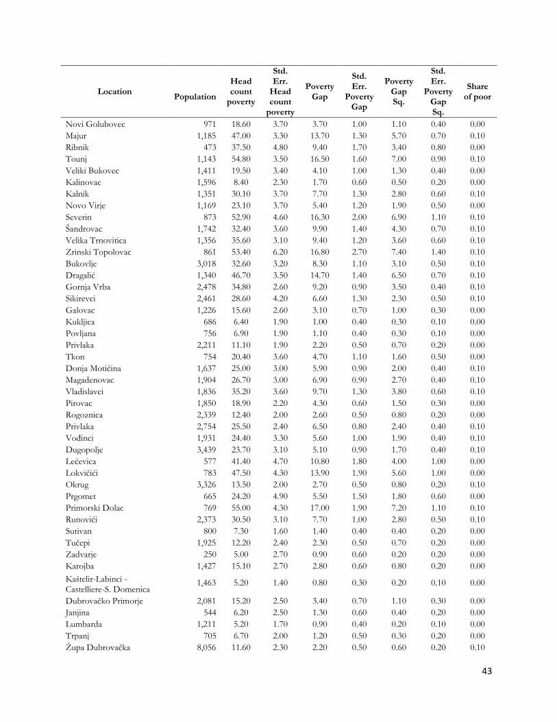
43

Location

Population

Head count

poverty

Std. Err.

Head count

poverty

Poverty Gap

Std. Err.

Poverty Gap

Poverty Gap Sq.

Std. Err.

Poverty Gap Sq.

Share of poor

Novi Golubovec 971 18.60 3.70 3.70 1.00 1.10 0.40 0.00

Majur 1,185 47.00 3.30 13.70 1.30 5.70 0.70 0.10

Ribnik 473 37.50 4.80 9.40 1.70 3.40 0.80 0.00

Tounj 1,143 54.80 3.50 16.50 1.60 7.00 0.90 0.10

Veliki Bukovec 1,411 19.50 3.40 4.10 1.00 1.30 0.40 0.00

Kalinovac 1,596 8.40 2.30 1.70 0.60 0.50 0.20 0.00

Kalnik 1,351 30.10 3.70 7.70 1.30 2.80 0.60 0.10

Novo Virje 1,169 23.10 3.70 5.40 1.20 1.90 0.50 0.00

Severin 873 52.90 4.60 16.30 2.00 6.90 1.10 0.10

Šandrovac 1,742 32.40 3.60 9.90 1.40 4.30 0.70 0.10

Velika Trnovitica 1,356 35.60 3.10 9.40 1.20 3.60 0.60 0.10

Zrinski Topolovac 861 53.40 6.20 16.80 2.70 7.40 1.40 0.10

Bukovlje 3,018 32.60 3.20 8.30 1.10 3.10 0.50 0.10

Dragalić 1,340 46.70 3.50 14.70 1.40 6.50 0.70 0.10

Gornja Vrba 2,478 34.80 2.60 9.20 0.90 3.50 0.40 0.10

Sikirevci 2,461 28.60 4.20 6.60 1.30 2.30 0.50 0.10

Galovac 1,226 15.60 2.60 3.10 0.70 1.00 0.30 0.00

Kukljica 686 6.40 1.90 1.00 0.40 0.30 0.10 0.00

Povljana 756 6.90 1.90 1.10 0.40 0.30 0.10 0.00

Privlaka 2,211 11.10 1.90 2.20 0.50 0.70 0.20 0.00

Tkon 754 20.40 3.60 4.70 1.10 1.60 0.50 0.00

Donja Motičina 1,637 25.00 3.00 5.90 0.90 2.00 0.40 0.10

Magadenovac 1,904 26.70 3.00 6.90 0.90 2.70 0.40 0.10

Vladislavci 1,836 35.20 3.60 9.70 1.30 3.80 0.60 0.10

Pirovac 1,850 18.90 2.20 4.30 0.60 1.50 0.30 0.00

Rogoznica 2,339 12.40 2.00 2.60 0.50 0.80 0.20 0.00

Privlaka 2,754 25.50 2.40 6.50 0.80 2.40 0.40 0.10

Vođinci 1,931 24.40 3.30 5.60 1.00 1.90 0.40 0.10

Dugopolje 3,439 23.70 3.10 5.10 0.90 1.70 0.40 0.10

Lećevica 577 41.40 4.70 10.80 1.80 4.00 1.00 0.00

Lokvičići 783 47.50 4.30 13.90 1.90 5.60 1.00 0.00

Okrug 3,326 13.50 2.00 2.70 0.50 0.80 0.20 0.10

Prgomet 665 24.20 4.90 5.50 1.50 1.80 0.60 0.00

Primorski Dolac 769 55.00 4.30 17.00 1.90 7.20 1.10 0.10

Runovići 2,373 30.50 3.10 7.70 1.00 2.80 0.50 0.10

Sutivan 800 7.30 1.60 1.40 0.40 0.40 0.20 0.00

Tučepi 1,925 12.20 2.40 2.30 0.50 0.70 0.20 0.00

Zadvarje 250 5.00 2.70 0.90 0.60 0.20 0.20 0.00

Karojba 1,427 15.10 2.70 2.80 0.60 0.80 0.20 0.00

Kaštelir-Labinci - Castelliere-S. Domenica

1,463 5.20 1.40 0.80 0.30 0.20 0.10 0.00

Dubrovačko Primorje 2,081 15.20 2.50 3.40 0.70 1.10 0.30 0.00

Janjina 544 6.20 2.50 1.30 0.60 0.40 0.20 0.00

Lumbarda 1,211 5.20 1.70 0.90 0.40 0.20 0.10 0.00

Trpanj 705 6.70 2.00 1.20 0.50 0.30 0.20 0.00

Župa Dubrovačka 8,056 11.60 2.30 2.20 0.50 0.60 0.20 0.10

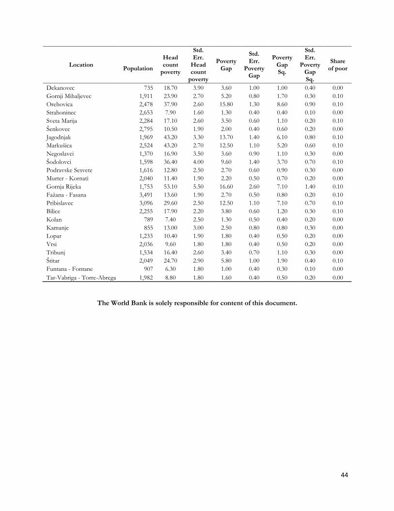
44

Location

Population

Head count

poverty

Std. Err.

Head count

poverty

Poverty Gap

Std. Err.

Poverty Gap

Poverty Gap Sq.

Std. Err.

Poverty Gap Sq.

Share of poor

Dekanovec 735 18.70 3.90 3.60 1.00 1.00 0.40 0.00

Gornji Mihaljevec 1,911 23.90 2.70 5.20 0.80 1.70 0.30 0.10

Orehovica 2,478 37.90 2.60 15.80 1.30 8.60 0.90 0.10

Strahoninec 2,653 7.90 1.60 1.30 0.40 0.40 0.10 0.00

Sveta Marija 2,284 17.10 2.60 3.50 0.60 1.10 0.20 0.10

Šenkovec 2,795 10.50 1.90 2.00 0.40 0.60 0.20 0.00

Jagodnjak 1,969 43.20 3.30 13.70 1.40 6.10 0.80 0.10

Markušica 2,524 43.20 2.70 12.50 1.10 5.20 0.60 0.10

Negoslavci 1,370 16.90 3.50 3.60 0.90 1.10 0.30 0.00

Šodolovci 1,598 36.40 4.00 9.60 1.40 3.70 0.70 0.10

Podravske Sesvete 1,616 12.80 2.50 2.70 0.60 0.90 0.30 0.00

Murter - Kornati 2,040 11.40 1.90 2.20 0.50 0.70 0.20 0.00

Gornja Rijeka 1,753 53.10 5.50 16.60 2.60 7.10 1.40 0.10

Fažana - Fasana 3,491 13.60 1.90 2.70 0.50 0.80 0.20 0.10

Pribislavec 3,096 29.60 2.50 12.50 1.10 7.10 0.70 0.10

Bilice 2,255 17.90 2.20 3.80 0.60 1.20 0.30 0.10

Kolan 789 7.40 2.50 1.30 0.50 0.40 0.20 0.00

Kamanje 855 13.00 3.00 2.50 0.80 0.80 0.30 0.00

Lopar 1,233 10.40 1.90 1.80 0.40 0.50 0.20 0.00

Vrsi 2,036 9.60 1.80 1.80 0.40 0.50 0.20 0.00

Tribunj 1,534 16.40 2.60 3.40 0.70 1.10 0.30 0.00

Štitar 2,049 24.70 2.90 5.80 1.00 1.90 0.40 0.10

Funtana - Fontane 907 6.30 1.80 1.00 0.40 0.30 0.10 0.00

Tar-Vabriga - Torre-Abrega 1,982 8.80 1.80 1.60 0.40 0.50 0.20 0.00

The World Bank is solely responsible for content of this document.