Geographic Poverty Traps?

A Micro Model of Consumption Growth in Rural China

Jyotsna JalanIndian Statistical Institute

New Delhi - 11 00 16. INDIA

jjalan@isid.ac.in

Martin RavallionWorld Bank

Washington DC - 20433. USAmravallion@worldbank.org

2

Summary

How important are neighborhood endowments of physical and human capital in

explaining diverging fortunes over time for otherwise identical households in a developing rural

economy? To answer this question we develop an estimable micro model of consumption

growth allowing for constraints on factor mobility and externalities, whereby geographic capital

can influence the productivity of a household’s own capital. Our statistical test has considerable

power in detecting geographic effects given that we control for latent heterogeneity in measured

consumption growth rates at the micro level. We find robust evidence of geographic poverty

traps in farm-household panel data from post-reform rural China. Our results strengthen the

equity and efficiency case for public investment in lagging poor areas in this setting.

Key words: Consumption growth, geographic externalities, nonstationary fixed effects, rural

China

JEL classification: D91, R11, Q12

3

Acknowledgements

The assistance and advice provided by staff of China's State Statistical Bureau in Beijing

and at various provincial and county offices are gratefully acknowledged. For useful comments

and discussions we thank the Journal’s two anonymous referees, Francisco Ferreira, Karla Hoff,

Aart Kraay, Kevin Lang, Marc Nerlove, Jaesun Noh, Danny Quah, Anand Swamy, and seminar

participants at the World Bank, University of Maryland College Park, Boston University, George

Washington University, Université des Sciences Sociales, Toulouse, the MacArthur

Foundation/World Bank Workshop on Emerging Issues in Development Economics, and the fifth

LACEA conference in Rio De Janerio. The financial support of the World Bank's Research

Committee (under RPO 681-39) is also gratefully acknowledged. These are the views of the

authors, and should not be attributed to the World Bank.

4

1. Introduction

Persistently poor areas have been a concern in many countries, including those

undergoing sustained aggregate economic growth. A casual observer traveling widely around

present day China will be struck by the disparities in levels of living, and signs that the robust

growth of relatively well off coastal areas has not been shared by poor areas inland, such as in the

southwest. China is not unusual; most countries have geographic concentrations of poverty; other

examples are the eastern islands of Indonesia, northeastern India, northwestern Bangladesh,

northern Nigeria, southeast Mexico and northeast Brazil.

Why do we see areas with persistently low living standards, even in growing economies?

One view is that they arise from persistent spatial concentrations of individuals with personal

attributes which inhibit growth in their living standards. This view does not ascribe a causal role

to geography per se; otherwise identical individuals will (by this view) have the same growth

prospects independently of where they live.

Alternatively one might argue that geography has a causal role in determining how

household welfare evolves over time. By this view, geographic externalities arising from local

public goods, or local endowments of private goods, entail that living in a well endowed area

means that a poor household can eventually escape poverty. Yet an otherwise identical household

living in a poor area sees stagnation or decline. If this is so, then it is important for policy to

understand what geographic factors matter to growth prospects at the micro level.

This paper tests for the existence of “geographic poverty traps”, such that characteristics

of a household’s area of residence ) it’s “geographic capital” ) entail that the household’s

consumption cannot rise over time, while an otherwise identical household living in a better

1 There are various administrative and other restrictions on migration, including registration andresidency requirements. For example, it appears to be rare for a rural worker who moves to an urban areato be allowed to enrol his or her children in the urban schools.

5

endowed area enjoys a rising standard of living. The paper also tries to identify the factors which

may lead to the emergence of such poverty traps. If borne out by empirical evidence, geographic

poverty traps suggest both efficiency and equity arguments for investing in poor areas, such as by

developing local infrastructure or by assisting labor export to better endowed areas.

The setting for our empirical work is post-reform rural China and we study the

determinants of consumption growth for farm households. We can rule out potential endogeneity

due to people choosing their locations because there was little or no geographic mobility of labor

in rural China at the time. Governmental restrictions on migration within China are part of the

reason.1 But there are other constraints on mobility. It is well known that household-level ties to

the village associated with traditional social security arrangements in underdeveloped rural

economies can be a strong disincentive against migration (see, for example, Das Gupta, 1987,

writing about rural India). Thin land markets, and the prospects for administrative re-allocation

of land, compound the difficulties in rural China. For these reasons, it is unusual for an entire

household to move from one rural area to another; the limited migration that is observed in rural

China and elsewhere appears to be mainly the temporary export of labor surpluses, primarily to

urban areas. Capital is probably more mobile than labor in China, although (again in common

with other developing economies) borrowing constraints appear to be pervasive, and financial

markets are poorly developed.

2 For evidence on China's regional disparities see Leading Group (1988), Lyons (1991), Tsui(1991), World Bank (1992, 1997), Knight and Song (1993), Rozelle (1994), Howes and Hussain (1994)

and Ravallion and Jalan (1996). On implications for policy (in the ligh of the results of the present paper)see Ravallion and Jalan (1999).

3 See Borjas (1995) on neighborhood effects on schooling and wages in the U.S. and Ravallionand Wodon (1999) on geographic effects on the level of poverty in Bangladesh.

6

One should not be surprised to find geographic differences in living standards in this

setting.2 Restrictions on labor mobility are one reason. But geography could also have a deeper

causal role in the dynamics of poverty in this setting. If geographic externalities alter returns to

private investment, and borrowing constraints limit capital mobility, then poor areas can self

perpetuate. Even with diminishing returns to private capital, poor areas will see low growth rates,

and possibly contraction.

However, testing for geographic poverty traps poses a number of problems. Using

aggregate geographic data, we can test for divergence, whereby poorer areas grow at lower rates.

But this is neither necessary nor sufficient for the existence of a geographic poverty trap.

Divergence may reflect either increasing returns to individual wealth, or geographic externalities,

whereby living in a poor area lowers returns to individual investments. Aggregate geographic

data cannot distinguish between the two causes.

Alternatively, cross-sectional micro data might be used to test for geographic effects on

living standards at one point in time.3 Such data can at best provide a snapshot of a household’s

welfare. One cannot say with statistical conviction that the observed geographic effects are not in

fact proxies for some unobserved household variables.

Both household panel data and geographic data are clearly called for to have any hope of

identifying geographic externalities in the growth process. But how should such data be

4 For example, suppose that the average wealth of an area is positively correlated with growthrates at household level, controlling for household wealth. This may be because some householdattribute relevant to growth, and positively correlated with average wealth, has been omitted. Better owneducation may yield higher growth rates, be correlated with wealth, and be spatially autocorrelated. Then average wealth in the area of residence could just be proxying for individual education.

5 Area characteristics (land quality) may be time-invariant. Alternatively, variables likepopulation density are typically only available from population censuses which are done infrequently,and so such variables must also be treated as time-invariant.

7

modeled? One might turn to the standard panel data model with time-invariant household fixed

effects. Allowing for latent heterogeneity in the household-level growth process will protect

against spurious geographic effects that arise from omitted geographic effects (such as latent

factors in the placement of government programs) or omitted non-geographic, but spatially

autocorrelated, household characteristics.4 However, standard panel-data techniques)like first-

differencing the data to eliminate the correlated unobserved household specific effects)wipe out

any hope of identifying impacts of the time-invariant geographic variables of interest, of which

there are likely to be many.5 In that case, the cure to the problem of latent heterogeneity leaves

an econometric model which is unable to answer many of the questions we started out with. Nor,

for that matter, is it obviously plausible that the heterogeneity in individual effects on growth

rates would in fact be time invariant; common macroeconomic and geo-climatic conditions might

well entail that the individual effects vary from year to year.

We propose an estimable micro model of consumption growth which can identify

underlying (including time-invariant) geographic effects while at the same time allowing for

latent heterogeneity in household-level growth rates. Our empirical work is motivated by an

adaptation of the Ramsey (1928) model of optimal consumption growth. The Ramsey model is

modified to allow geographic effects on the marginal product of own capital in the presence of

6 Analogously to the role of external (economy-wide) knowledge on firm productivity in theRomer (1986) model.

8

constraints on capital mobility. Our econometric model uses longitudinal observations of growth

rates at the micro level collated with other micro and geographic data. Following Holtz-Eakin,

Newey and Rosen (1988), our panel data model allows for individual effects with nonstationary

impacts. The standard fixed effects model is encompassed as a testable restricted form. If it is

rejected in favor of nonstationary effects then we are able to identify impacts of time-invariant

geographic capital on consumption growth at micro level while still allowing for latent

heterogeneity in measured growth rates. We implement the approach using farm-household panel

data for rural areas of southern China over 1985-90.

The following section outlines our theoretical model of consumption growth, while

section 3 gives the econometric model. Section 4 describes our data while section 5 presents our

results. Section 6 summarizes our conclusions.

2. Theoretical model

Our empirical work is motivated by extending the classic Ramsey model of intertemporal

consumer equilibrium to include production by a farm-household facing geographic externalities

in its production process. We hypothesize that output of the farm household is a concave function

of various privately-provided inputs, but that output also depends positively and non-separably

on the level of geographic capital, as described by characteristics of the area of residence.6 We

do not assume perfect capital mobility. In competitive equilibrium, this would entail that

marginal products of private capital (net of depreciation rates) are equalized across all farm-

households at a common rate of interest. Then (under the other assumptions of the standard

9

(1)

Ramsey model) differences in endowments of geographic capital will not entail differences in

consumption growth rates, even if the geographic differences alter the marginal product of

private capital. Levels of private capital will adjust to restore equilibrium. To assume perfect

capital mobility would thus preclude what is arguably the main source of the geographic poverty

traps that we hope to test for. Although limited financial transactions exist, perfect capital

mobility is also implausible in this setting.

The household operates a farm which produces output by combining labor and own

capital (which can be interpreted as a composite of land, physical capital and human capital)

under constant returns to scale. There are constraints on access to credit, with the effect that

capital is not perfectly mobile between farm-households. Thus diminishing returns to private

capital set in at the farm-household level. The household’s farm output also depends on a vector

of geographic variables, G, reflecting external effects on own-production. Output per worker or

person is F(K, G) where K denotes capital per worker. Output can be consumed, invested

(including offsets for depreciation), or used to repay debt. We make the standard assumption that

the household maximizes an inter-temporally additive utility integral:

where is the intertemporal elasticity of substitution, C is consumption, and D is the subjective

rate of time preference.

10

(2)

The derivation of the optimal rate of consumption growth under these assumptions then

follows from standard methods for dynamic optimization. It can be shown that the optimal rate

of consumption growth satisfies the Euler equation:

where is the rate of depreciation plus labor augmenting technical progress.

The key feature of this equation for our purpose is that geographic externalities can

influence consumption growth rates at the farm-household level, through effects on the marginal

product of own capital. The model permits values of G such that the optimal consumption

growth rate is negative; given G, output gains from individually optimal investments may not be

sufficient to cover and so consumption falls.

There are other ways in which geographic effects on consumption growth might arise, not

captured by the above model. For example, we could also allow geographic variables to

influence utility at a given level of consumption, by making the substitution parameter and the

discount rate functions of G. While our empirical model will allow us to test for geographic

effects on consumption growth at the micro level it will not allow us to identify the precise

mechanism linking area characteristics to growth.

11

(3)

(4)

3. Econometric model

The Euler equation in (2) motivates an empirical model in which the growth rate of

household consumption depends on both the household’s own capital and on its geographic

capital. Data are available for a random sample of N households observed over T dates, where T

is at least three (for reasons that will soon be obvious). Let git denote the expected value of the

growth path for i at t (git is thus the value of g(t) in discrete time) and let lnCit be the measured

growth-rate of consumption for household i in time period t. Rather than assume that lnCit=git

we allow for measurement errors and lagged effects according to an ad hoc adjustment model:

where is an error term. This can be taken to include idiosyncratic effects on the marginal

product of own capital and the rate of time preference, as well as measurement errors in growth

rates. Our empirical model for git is:

where xit is a ( k x 1) vector of time-varying explanatory (geographic and household) variables,

and zi is a ( p x 1) vector of exogenous time-invariant explanatory (geographic and household)

variables.

There are likely to be differences in own-capital endowments, and other parameters of

utility and production functions, which one cannot hope to fully capture in the data available.

There are also likely to be omitted geographic variables, such as latent political or economic

factors influencing the placement of observed governmental programs. Furthermore, it is likely

12

(5)

that these unobserved household and geographic variables will be correlated with the observed

geographic variables, leading to biases in OLS estimates of the parameters of interest. So in

estimating equation (3), we assume that the error term includes a household-specific fixed

effect (which may also include unobserved geographic effects) correlated with the regressors as

well as an i.i.d. random component which is orthogonal to the regressors and is serially

uncorrelated.

The existence of economy-wide factors (including covariate shocks to agriculture)

suggests that the impact of the heterogeneity need not be constant over time. For example, there

may be a latent effect such that some farmers are more productive, but this matters more in a bad

agricultural year than a good one. This could also hold for observed sources of heterogeneity. In

particular, some or all of the zi variables may well have time-varying effects, so that includes

deviations from the time mean impacts, ( )zi, in obvious notation. This would also entail a

correlation between the latent household-specific effect and the regressors, as well as

nonstationarity in the latent effects. However, the time varying parameters are clearly not

identifiable; only time-mean impacts are recoverable.

To allow for nonstationarity in the impacts of the individual effects we follow Holtz-

Eakin et al., (1988) in decomposing the composite error term as:

7 An alternative estimation method is the dynamic random effects estimator developed byBhargava and Sargan (1982). However, this method assumes that at least some of the time-varyingvariables are uncorrelated with the unobserved individual specific effect.

8 Also see Chamberlain (1984) and Ahn and Schmidt (1994) for alternative quasi-differencingtransformations.

13

(6)

where uit is the i.i.d. random variable, with mean 0 and variance 2u , and is a time-invariant

effect that is not orthogonal to the regressors. The following assumptions are made about the

error structure:

Since the composite error term in equation (5) is not orthogonal to the regressors, estimating

(3) by OLS will give inconsistent estimates. Serial independence of uit is a strong assumption; for

example, measurement error in the levels of consumption can generate first-order (negative)

serial correlation in uit. However, while serial independence of uit is sufficient for our estimation

strategy, it is not necessary; we will perform diagnostic tests on the necessary condition (below).

In standard panel data models, the “nuisance” variable is eliminated by estimating the

model in first differences or by taking time-mean deviations (when there is no lagged dependent

variables in the model).7 However, given the temporal pattern of the effect of on lnCit, we

cannot use these transformations to eliminate the fixed effect. We use instead quasi-differencing

techniques, following Holtz-Eakin et. al. (1988).8 Substituting equation (4) and (5) into (3) and

lagging by one period we get:

14

(7)

(8)

(9)

(10)

Define rt = / . Multiplying equation (7) by rt and subtracting from equation (3):

Notice that even if we had assumed that the measured growth rate is the long-run value for that

date ( =0), a dynamic specification would still be called for as long as the latent effects are time

varying. This is generated by the quasi-differencing.

Consider the identification of the original parameters. Equation (8) is a function of the

ratio rt of the coefficients of the individual effects. The level of these coefficients are not

identified. Rewriting equation (8) as:

where

In our model, the only time-varying parameter is the ratio of the coefficients of the individual

effects, rt. Thus all the original parameters (excepting the levels of the coefficients associated

15

with the individual effect) can easily be recovered without any further restrictions on the number

of estimable time periods.

For our purposes, an advantage of the above approach over the standard fixed effects set-

up is that coefficients on the time-invariant regressors are identified. Intuitively this is achieved

by relaxing the usual cross-equation restrictions that the coefficients on the time-invariant

variables must be constant over time. Thus our method simultaneously allows us to control for

latent heterogeneity while still identifying the impacts of time invariant factors including the

geographic variables of interest.

This general specification can be tested against the restriction of the standard fixed-

effects model, namely that for all t. We recognize that standard chi-square asymptotic tests

are not applicable in this case since under the null hypothesis, H0: rt=1, the parameters associated

with the constant and the time-invariant variables are not identified. We follow a suggestion by

Godfrey(1988) (following Davies, 1977, 1987) to test for the presence of non-stationary fixed

effects in our data when several parameters vanish under the null hypothesis. We set " and . to

some constants "0 and .0 respectively. When we test the null hypothesis, "0(1-rt)=.0(1-rt)=0, the

statistic LM("0, .0) -P2(1) whatever the choices of ("0, .0). Godfrey (1988) states that in small

samples, power of this simple test will be a concern but in our case with a cross-sectional sample

of 5,600 households this is not an issue.

In estimating equation (8) we must allow for the fact that one of the regressors, lnCit -1,

is correlated with the error term, uit-rtuit-1 (although the error term is by construction orthogonal

to xit and zi). One can estimate equation (8) by Generalized Method of Moments (GMM) using

9 There is some debate regarding the choice of the optimal moment conditions (and henceinstruments) to estimate dynamic panel data models efficiently (Ahn and Schmidt, 1995; Blundell andBond, 1997). In this discussion, the primary concern is with respect to the use of lagged levelinstruments especially in cases where the estimated coefficient of the lagged dependent variable is closeto unity. In a related paper, Binder, Hsiao and Pesaran (2000) suggest a maximum likelihood estimator tocircumvent the problem of unit-roots in short panels. Their methods however, can not be easily extendedto the GMM framework. In our case, the estimable model is in differences. Further, the coefficientestimate for the lagged difference dependent variable is different from unity.

10 Note that there is some first-order serial correlation introduced in the model due to the quasi-differencing. This means that log consumptions lagged once are not valid instruments.

16

differences and/or levels of log consumptions lagged twice (or higher) as instruments for lnCit-

1. (The Appendix provides a more complete exposition of the estimation method.) The essential

condition to justify this choice of instruments is that the error term in (8) is second-order serially

independent. That is implied by serial independence of uit.9

To ensure that our estimation strategy is valid we perform three diagnostic tests. First, we

test whether latent individual specific effects are present in our data. We construct a Hausman-

type test where the null hypothesis that the GLS model is the correct one is tested against the

latent variable model. Second, we follow Arellano and Bond (1991) in constructing an over-

identification test to ensure that our instruments are consistent with the data and are indeed

exogenous. Thirdly, we perform the Arellano-Bond second-order serial correlation test, given

that the consistency of the GMM estimators for the quasi-differenced model depends on the

assumption that the composite error term in (8) is second-order serially independent, as discussed

above.10 Lack of second-order serial correlation and the non-rejection of the over-identification

test support our choice of instruments.

Note also that quasi-differencing the data to eliminate the unobserved household effects

will also remove any remaining latent geographic effects provided the ‘s are the same for the

17

county and the individual specific effects. However this need not be the case in our data. To test

against the presence of remaining latent area effects, we regressed the estimated residuals against

a set of geographic dummies and tested their joint significance.

4. Data

The farm-household level data were obtained from China’s Rural Household Survey

(RHS) done by the State Statistical Bureau (SSB). A panel of 5,600 farm households over the

six-year period 1985-90 was formed for four contiguous provinces in southern China, namely

Guangdong, Guangxi, Guizhou, and Yunnan. The latter three provinces form southwest China,

widely regarded as one of the poorest regions in the country. Guangdong on the other hand is a

relatively prosperous coastal region (surrounding Hong Kong). In 1990, 37%, 42% and 34% of

the populations of Guangxi, Guizhou and Yunnan, respectively, fell below an absolute poverty

line which only 5% of the population of Guangdong could not afford (Chen and Ravallion,

1996). Also the rural southwest appears to have shared little in China’s national growth in the

1980s. For the full sample over 1985-90, consumption per person grew at an average rate of only

0.70% per annum; for Guangdong, however, the rate of growth was 3.32%. Between 1985 and

1990, 54% of the sampled households saw their consumption per capita increase while the rest

experienced decline.

The data appear to be of good quality. Since 1984 the RHS has been a well-designed and

executed survey of a random sample of households in rural China (including small-medium

towns), with unusual effort made to reduce non-sampling errors (Chen and Ravallion, 1996).

Sampled households fill in a daily diary on expenditures and are visited on average every two

weeks by an interviewer to check the diaries and collect other data. There is also an elaborate

11 Constructing the panel from the annual RHS survey data proved to be more difficult thanexpected since the identifiers could not be relied upon. Fortunately, virtually ideal matching variableswere available in the financial records, which gave both beginning and end of year balances. Therelatively few ties by these criteria could easily be broken using demographic (including age) data.

12 For further details on the poverty lines see Chen and Ravallion (1996). Note that our test foromitted geographic effects can be interpreted as a test for mis-measurement in our deflators.

18

system of cross-checking at the local level. The consumption data from such an intensive survey

process are almost certainly more reliable than those obtained by the common cross-sectional

surveys in which the consumption data are based on recall at a single interview. For the six year

period 1985-90 the survey was also longitudinal, returning to the same households over time.

While this was done for administrative convenience (since local SSB offices were set up in each

sampled county), the panel can still be formed.11

The consumption measure includes imputed values for consumption from own

production valued at local market prices, and imputed values of the consumption streams from

the inventory of consumer durables (Chen and Ravallion, 1996). Poverty lines designed to

represent the cost at each year and in each province of a fixed standard of living were used as

deflators. These were based on a normative food bundle set by SSB, which assures that average

nutritional requirements are met with a diet that is consistent with Chinese tastes. This food

bundle is then valued at province-specific prices. The food component of the poverty line is

augmented with an allowance for non-food goods, consistent with the non-food spending of

those households whose food spending is no more than adequate to afford the food component of

the poverty line.12

The household data were collated with geographic data at three levels: the village, the

county, and the province. At village level, we have data on topography (whether the village is on

13 While the county administrative records and the county yearbooks cover rural areasseparately, the census county data does not distinguish between the rural and urban areas. However,given that the objective of including the county characteristics is to proxy for the initial level of progressin a particular county relative to another, the aggregate county indicators should be reliable indicators forthe differences in socio-economic conditions across the counties.

19

plains, or in hills or mountains, and whether it is in a coastal area), urbanization (whether it is a

rural or suburban area), ethnicity (whether it is a minority group village), whether or not it is a

border area (three of the four provinces are at China’s external border), and whether the village is

in a revolutionary base area (areas where the Communist Party had established its bases prior to

1949). At the county level we have a much larger data base drawn from County Administrative

Records (from the county statistical year books for 1985-90) and from the 1982 Census.13 These

cover agriculture (irrigated area, fertilizer usage, agricultural machinery in use), population

density, average education levels, rural non-farm enterprises, road density, health indicators, and

schooling indicators. At the province level, we simply include dummy variables for the

province. All nominal values are normalized to 1985 prices.

The survey data also allow us to measure a number of household characteristics. A

composite measure of household wealth can be constructed, comprising valuations of all fixed

productive assets, cash, deposits, housing, grain stock, and consumer durables. We also have

data on agricultural inputs used, including landholding. To allow for differences in the quality

and quantity of family labor (given that labor markets are thin in this setting) we let education

and demographics influence the marginal product of own capital; these may also influence the

rates of intertemporal substitution and/or time preference. We have data on the size and

demographic compositions of the households, and levels of schooling.

Table 1 gives descriptive statistics on the variables.

20

(11)

5. Results

We begin with a simple specification in which the only explanatory variables are initial

wealth per capita, both at household and county levels. This model is too simple to be believed,

but it will help as an expository device for understanding a richer model later.

5.1 A simple expository model

Suppose that the only two variables that matter to the long run consumption growth rate

are initial household wealth per capita (HW) and mean wealth per capita in the county of

residence (CW). The long-run growth rate for household i is then:

This is embedded in the dynamic empirical model, as described in section 3.

Using lagged first differences of log consumption as instruments, the GMM estimate of

this model gives rt values of 0.601, 0.220, and 0.558 for 1988 to 1990 respectively. Using

standard errors which are robust to any cross-sectional heteroscedasticity that might be present in

the data, the corresponding t-ratios are 7.84, 8.40 and 6.63. The estimated equation for the

balanced growth rate is (t-ratios in parentheses, also based on robust standard errors):

g(HW,CW) = (- 0.278 - 0.0221lnHW + 0.0602lnCW)/1.172 (12) (6.02) (4.52) (7.27) (57.46)

This is interpretable as the estimate of equation (2) implied by this specification, where HW is

interpreted as a measure of K and CW as a measure of G.

21

Thus we find that consumption growth rates at the farm-household level are a decreasing

function of own wealth, and an increasing function of average wealth in the county of residence,

controlling for latent heterogeneity. We can interpret equation (12) in terms of the model in

section 2. The time preference rate and elasticity of substitution are not identified. Nonetheless,

given that the substitution parameter is positive, we can infer from (12) that the marginal product

of own capital is decreasing with respect to own capital, but increasing with respect to

geographic capital. However, there are other possible interpretations; for example, credit might

well be attracted to richer areas, or discount rates might be lower.

Notice that the sum of the coefficients on lnCW and lnHW in (12) is positive. Averaging

(12) over all households in a given county, we thus find aggregate divergence; counties with

higher initial wealth will tend to see higher average growth rates. That is indeed what one finds

in aggregate county data for this region of China (Ravallion and Jalan, 1996). This is due entirely

to geographic externalities, rather than increasing returns to own wealth at farm-household level.

5.2 A richer model

While the above specification is useful for expository purposes, we now want to extend

the model by adding a richer set of both geographic and household-level variables. Table 1 gives

the descriptive statistics of the explanatory variables to be used in the extended specification.

We first estimated a first order dynamic consumption growth model as indicated by

equation (3). However, the Wald statistic to test the significance of the coefficient associated

with the lagged dependent variable ( ) had a p-value of 0.39. So we opted for the parsimonious

model where the dynamics are introduced only via the quasi-differencing. An advantage of this

is that we gain an extra period for the estimation.

14 Given that our preferred estimated equation is static, we can construct a Hausman type testbecause the parameter estimates are consistent under both the null and the alternative hypothesis. In our

specification we can also simply test the null hypothesis of for all t which is also rejected by aWald test.

15 The null hypothesis for all t, where are set to their estimatedvalues, is rejected by a Wald test with a p-value of 0.035 for the associated Chi-square statistic.

16 We estimated a model where the household variables were assumed to be exogenous (basemodel). Next we estimated an alternative model where it was assumed that the time-varying householdvariables are endogenous, for which we used lagged values of the endogenous variables as instruments.We then constructed likelihood ratio tests to test the base model against this model (Hall, 1993; Ogaki,1993).

17 Even though we include a number of time-invariant household variables as regressors in themodel, the correlation matrix associated with these variables indicate the highest correlation to be around0.7, suggesting that multi-collinearity is not a serious problem in our sample and model.

22

Table 2 reports our GMM estimates of the extended model. On testing the fixed effects

model against a model with no latent effects (stationary or non-stationary), a Hausman-type test

based on the difference between the quasi-differenced model and the GLS model gave a

=63.1 which is significant at the 5% level.14 Again the conventional fixed effects model is

firmly rejected in favor of the specification with time-varying coefficients.15 This also means that

we can estimate the impacts of the time-invariant geographic (and non-geographic) variables.

Our model also includes time-varying household variables (Table 1). The question arises

as to whether to treat these variables as exogenous or endogenous. The model where the

household variables are treated as exogenous was summarily rejected in favor of the model

where the time-varying household variables are endogenous.16 Hence, Table 2 reports estimates

where the time-varying household variables are treated as endogenous. All the time-invariant

variables—county and household—are treated as exogenous.17

The over-identification test, and the second-order serial correlation test indicate that the

instruments used in the GMM estimation are valid. The over-identification test has a p-value of

23

0.9 and the second-order serial correlation test statistic has a p-value of 0.5. Furthermore, there

appear to be no remaining latent area effects in the residuals of the estimated model. The F-test

statistic is F101,22474 = 0.95 which is not significant.

Many of the geographic variables are significant. Living in a mountainous area lowers the

long run rate of consumption growth, while living on the plains raises it (“hills” is the left out

category). Natural conditions for agriculture tend to be better in the plains than mountains or

hills. Both of the geographic variables measuring the extent of modernization in agriculture (farm

machinery usage per capita and fertilizer usage per acre) have highly significant positive impacts

on individual consumption growth rates. The two health-related variables (infant mortality rate

and medical personnel per capita) indicate that consumption growth rates at the farm-household

level are significantly higher in generally healthier areas. A higher incidence of employment in

non-farm commercial enterprises in a geographic area entails a higher growth rate at the

household level for those living there. There is a highly significant positive effect of higher road

density in an area on consumption growth. Historically favored “revolutionary base” areas have

higher long run growth rates controlling for the other variables.

Consistent with the simpler model we started with, there is a strong tendency for the

geographic variables to be either neutral or “divergent”, in that households have higher

consumption growth rates in better endowed areas. This suggests that these geographic

characteristics tend to increase the marginal product of own capital.

This is in marked contrast to the household-level variables. In addition to allowing for

latent farm-household level effects on consumption growth, we included a number of household

level characteristics related to land and both physical and human capital endowments. These

24

effects tend to be neutral or convergent. We find that farm-households with higher expenditure

on agricultural inputs per unit land area (an indicator of the capital intensity of agriculture)

tended to have lower subsequent growth rates. Fixed productive assets per capita do not,

however, emerge as significant; it may well be that the density of agricultural inputs is the better

indicator of own-farm capital. Amongst the other household characteristics, there are a number

of significant demographic variables; larger and younger households tend to have higher

consumption growth rates. This may reflect the thinness of agricultural labor markets in rural

China, so that demographics of the household influence the availability of labor for farm work.

5.3 Do geographic poverty traps occur within the bounds of the data?

The above results are consistent with geographic poverty traps. But do such traps actually

occur within the bounds of these data? In terms of the theoretical model in section 2, while one

might find that higher endowments of geographic capital raise the marginal product of own

capital at the farm-household level, it may still be the case that no area has so little geographic

capital to entail falling consumption.

To address this issue, consider first our simple model in section 5.1. The poverty trap

level of county wealth can be defined as CW * such that g(HW, CW *)= 0 for given HW. Figure 1

gives CW * for each value of HW. The figure also gives the data points. Clearly there is a large

subset of the data for which CW is too low, given HW, to permit rising consumption. Consider,

for example, two households both with the sample mean of lnHW, which is 6.50 (with a standard

deviation of 0.61). From equation (12), lnCW* = 7.01 at this level of household wealth. So if

one of the two households happens to live in a county with lnCW = 7.02 or higher it will see

25

rising consumption over time in expectation, while if the other lives in a county with lnCW =

7.00 or lower it will see falling consumption, even though its initial personal wealth is the same.

We can ask the same question for the richer model. We calculate the critical value of

each geographic variable at which consumption growth is zero while holding all other

(geographic and non-geographic) variables constant. While we cannot graph all the possible

combinations in this multidimensional case (as in Figure 1), let us fix other variables at their

sample mean values. The critical values implied by our results are given in Table 3.

We find, for example, that positive growth in consumption requires that the density of

roads exceeds 6.5 square kilometers per 10,000 people, with all other variables evaluated at mean

points (Table 3). In all cases, the critical value at which the geographic poverty trap arises is

within one standard deviation of the sample mean for that characteristic.

Geographic poverty traps are clearly well within the bounds of these data.

6. Conclusions

Mapping poverty and its correlates could well be far more than a descriptive tool)it may

also hold the key to understanding why poverty persists in some areas, even with robust

aggregate growth. That conjecture is the essence of the theoretical idea of a geographic poverty

trap. But are such traps of any empirical significance?

That is a difficult question to answer. Aggregate regional growth empirics cannot do so,

since aggregation confounds the external effects that create geographic poverty traps with purely

internal effects. And, without controlling for latent heterogeneity in the micro growth process, it

is hard to accept any test for geographic poverty traps based on micro panel data. In a regression

for consumption growth at the household level, significant coefficients on geographic variables

26

may simply pick up the effects of omitted spatially-autocorrelated household characteristics. Yet

the standard treatments for fixed effects in micro panel-data models make it impossible to

identify the impacts of the many time-invariant geographic factors that one might readily

postulate as leading to poverty traps. Given the potential policy significance of geographic

poverty traps, it is worth searching for a convincing method to test for them.

We have offered a test. This involves regressing consumption growth at the household

level on geographic variables, allowing for nonstationary individual effects in the growth rates.

By relaxing the restriction that the individual effects have the same impacts at all dates, the

resulting dynamic panel-data model of consumption growth allows us to identify external effects

of fixed or slowly changing geographic variables.

On implementing the test on a six-year panel of farm-household data for rural areas of

southern China, we find strong evidence that a number of indicators of geographic capital have

divergent impacts on consumption growth at the micro level, controlling for (observed and

unobserved) household characteristics. The main interpretation we offer for this finding is that

living in a poor area lowers the productivity of a farm-household’s own investments, which

reduces the growth rate of consumption, given restrictions on capital mobility.

With only six years of data it would clearly be hazardous to give our findings a “long-

run” interpretation (though six-years is relatively long for a household panel). Possibly we are

observing a transition period in the Chinese rural economy. However, our results do suggest that

there were areas in this part of rural China in this period which were so poor that the

consumptions of some households living in them were falling even while otherwise identical

27

households living in better off areas enjoyed rising consumptions. Within the period of analysis,

the geographic effects were strong enough to imply poverty traps.

What geographic characteristics create poverty traps? We find that there are publicly

provided goods in this setting, such as rural roads, which generate non-negligible gains in living

standards. (And since we have allowed for latent geographic effects, the effects of these

governmental variables cannot be ascribed to endogenous program placement.) We also find that

the aspects of geographic capital relevant to consumption growth embrace both private and

publicly provided goods and services. Private investments in agriculture, for example, entail

external benefits within an area, as do “mixed” goods (involving both private and public

provisioning) such as health care. The prospects for growth in poor areas will then depend on the

ability of governments and community organizations to overcome the tendency for under-

investment that such geographic externalities are likely to generate.

28

(A1)

(A2)

(A3)

(A4)

Appendix: GMM estimation of the micro growth model

The estimation procedure entails stacking the equations in (8) to form a system, with one

equation for each year. For T=6, the system of equations to be estimated is as follows:

In these equations, (t=3,4,5,6) is the error term u it-rt uit -1 , xit is the vector of time-varying

explanatory variables, zi the vector of time invariant variables, and bt = [", $, >, (, rt] is the

parameter vector. Note that not all the b’s vary with time, implying certain cross-equation

restrictions on the parameters. It is convenient to write the model in the compact form:

where is a (T-2)x1 vector for household i.

The GMM procedure estimates the parameters bt by minimizing the criterion function:

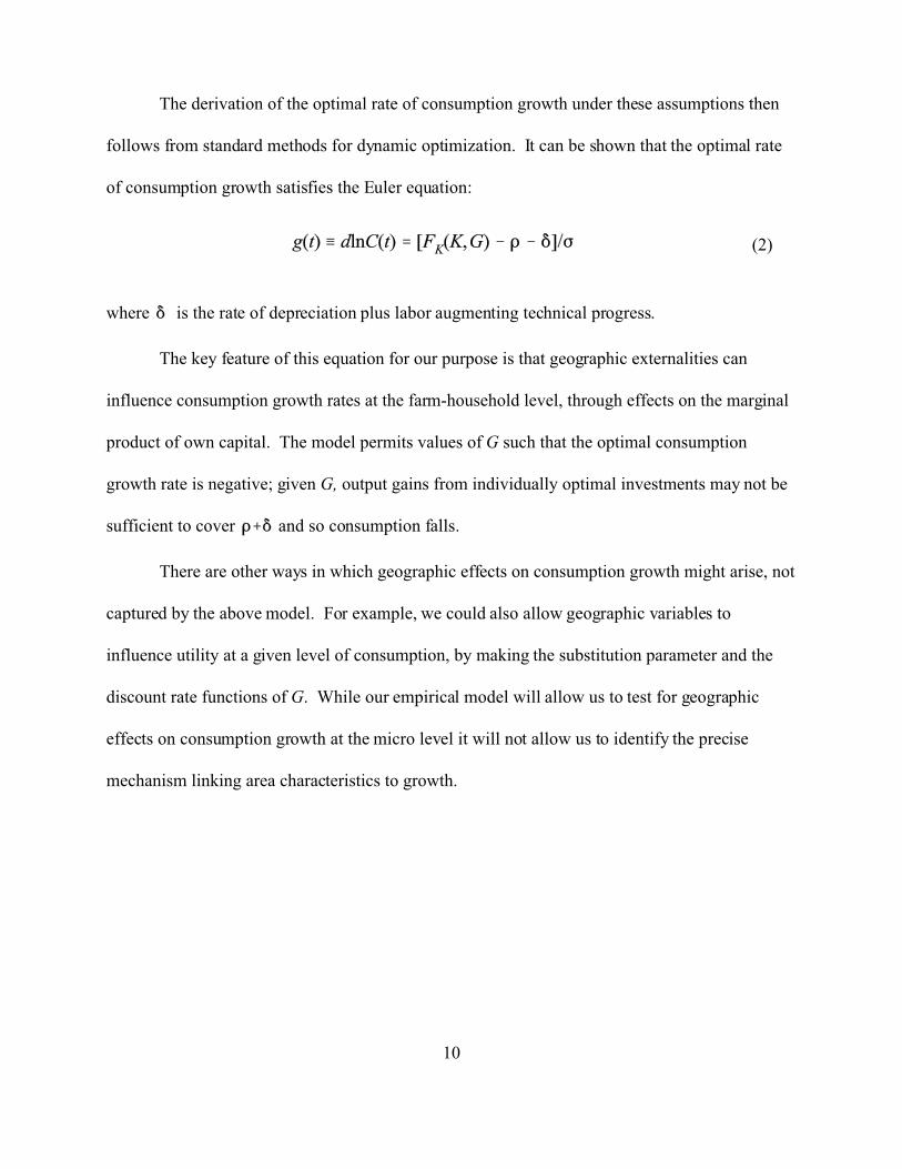
where the (l x l) weighting matrix AN is positive definite, and where the (l x 1) vector of sample

orthogonality conditions is given by:

29

(A5)

where wi is a ((T-2) x l) vector of l instruments. Heteroscedasticity is likely to exist across the

cross-sections. We use White’s approach to correct for this. The optimal weighting matrix is

thus the inverse of the asymptotic covariance matrix:

where is the vector of the estimated residuals. These GMM estimates yield parameter

estimates that are robust to heteroscedasticity.

The first-order conditions of minimizing the non-linear equation QNT(b), does not provide

us with an explicit solution. We must thus use a numerical optimization routine to solve for .

All the computations can be done using standard software such as EVIEWS and GAUSS.

30

References

Ahn, S.C., Y.H. Lee and P. Schmidt (1994), “GMM Estimation of a Panel Data Regression

Model with Time-varying Individual Effects”, mimeo, Arizona State University.

Ahn, S.C. and P. Schmidt (1995), “Efficient Estimation of Models for Dynamic Panel Data”,

Journal of Econometrics, 68, 5-27.

Arellano, M. and S. Bond (1991), "Some Tests of Specification for Panel Data: Monte- Carlo

Evidence and An Application to Employment Equation", Review of Economic Studies,

58, 277-298.

Bhargava, A. and J. D. Sargan (1983), “Estimating Dynamic Random Effects Models from Panel

Data Covering Short Time Periods”, Econometrica, 51, 1635-1659.

Binder, M., C. Hsiao, and M. Hashem Pesaran (2000), “Estimation and Inference in Short Panel

Vector Autoregressions with Unit Roots and Cointegration”, Bank of Spain Working

Paper #0005, Madrid, Spain

Blundell, R. and S. Bond (1997), “Initial Conditions and Moment Restrictions in Dynamic Panel

Data Models,” University College London Discussion Paper Series #97/07, London,

University College.

Borjas, G. (1995), "Ethnicity, Neighborhoods, and Human Capital Externalities", American

Economic Review, 85, 365-380.

Chamberlain, G. (1984), “Panel Data” in Z.Grilliches and M. Intrilligator (eds.), Handbook of

Econometrics, Vol. 2, Amsterdam, North-Holland.

Chen, S. and M. Ravallion (1996), "Data in Transition: Assessing Rural Living

Standards in Southern China", China Economic Review, 7, 23-56.

31

Das Gupta, M. (1987), “Informal Security Mechanisms and Population Retention in Rural India”,

Economic Development and Cultural Change, 36, 101-120.

Davies, R.B. (1977), “Hypothesis Testing when a Nuisance Parameter is Unidentified Under the

Alternative”, Biometrika, 64, 247-254.

Davies, R.B. (1987), “Hypothesis Testing when a Nuisance Parameter is Unidentified Under the

Alternative”, Biometrika, 74, 33-43.

Godfrey, L.G. (1988), Misspecification Tests in Econometrics, Cambridge University Press,

Cambridge.

Hall, A. (1993), "Some Aspects of Generalized Method of Moments Estimation", in G. S.

Maddala, C. R. Rao, and H. D. Vinod (eds.), Handbook of Statistics, Volume 11,

Amsterdam, North-Holland.

Holtz-Eakin, D., W. Newey and H. Rosen (1988), “Estimating Vector Autoregressions withPanel

Data”, Econometrica, 56, 1371-1395.

Holtz-Eakin, D. (1988), “ Testing for Individual Effects using Panel Data”, Journal of

Econometrics, 39, 297-307.

Howes, S. and A. Hussain (1994), “Regional Growth and Inequality in Rural China”, Working

Paper EF 11, London, London School of Economics.

Jalan, J. and M. Ravallion (1998), “Are There Dynamic Gains from a Poor-Area

Development Program?”, Journal of Public Economics, 67, 65-85.

Knight, J. and S. Lina (1993), “The Spatial Contribution to Income Inequality in Rural China”,

Cambridge Journal of Economics, 17, 195-213.

32

Leading Group (1988), Outlines of Economic Development in China's Poor Areas, Office of the

Leading Group of Economic Development in Poor Areas Under the State Council,

Agricultural Publishing House, Beijing.

Lyons, T. (1991), “Interprovincial Disparities in China: Output and Consumption, 1952-1987", Economic Development and Cultural Change, 39, 471-506.

Ogaki, M. (1993), "Generalized Method of Moments: Econometric Applications", in G. S.

Maddala, C. R. Rao, and H. D. Vinod (eds.), Handbook of Statistics, Volume 11,

Amsterdam, North-Holland.

Ramsey, F. (1928), “A Mathematical Theory of Saving”, Economic Journal, 38, 543-559.

Ravallion, M. and J. Jalan (1996), “Growth Divergence due to Spatial Externalities”, Economics

Letters, 53, 227-232.

Ravallion, M. and J. Jalan (1999),“China’s Lagging Poor Areas”, American Economic Review

(Papers and Proceedings), 89, 301-305.

Ravallion, M. and Q. Wodon (1999), “Poor Areas, Or Only Poor People?”, Journal of

Regional Science, 39, 689-711.

Romer, P. M. (1986), "Increasing Returns and Long-Run Growth", Journal of

Political Economy, 94, 1002-1037.

Rozelle, S. (1994), ”Rural Industrialization and Increasing Inequality: Emerging Patterns in

China's Reforming Economy”, Journal of Comparative Economics, 19, 362-391.

Tsui, K. Y. (1991), “China's Regional Inequality, 1952-1985", Journal of Comparative

Economics, 15, 1-21.

World Bank (1992), China: Strategies for Reducing Poverty in the 1990s, World Bank,

Washington DC.

33

_________ (1997), China 2020: Sharing Rising Incomes, World Bank, Washington DC.

34

Table 1: Descriptive statistics

Variable Summary statistics

Mean Standard

deviation

Dependent variable

Average % growth rate of consumption, 1986-90 0.7004 28.5290

Geographic variables

Proportion of sample in Guangdong 0.2286 0.4199

Proportion of sample in Guangxi 0.2442 0.4296

Proportion of sample in Yunnan 0.2029 0.4021

Proportion living in a revolutionary base area 0.0259 0.1587

Proportion of counties sharing a border with a foreign

country

0.1547 0.3616

Proportion of villages located on the coast 0.0307 0.1724

Proportion of villages in which there is a

concentration of ethnic minorities

0.2562 0.4365

Proportion of villages that have a mountainous terrain 0.4415 0.4966

Proportion of villages located in the plains 0.2171 0.4122

Fertilizers used per cultiv. area (tonnes per sq.km) 11.8959 6.4937

Farm machinery used per capita (horsepower)a 158.5453 151.2195

Cultivated area per 10,000 persons (sq km) 13.0603 3.2622

Population density (log) 8.2264 0.3786

Proportion of illiterates in the 15+ population (%) 34.8417 15.8343

Infant mortality rate (per 1,000 live births) 40.4600 23.3683

Medical personnel per 10,000 persons 8.0576 5.0205

Pop. employed in commercial (non-farm) enterprises

(per 10,000 persons)

117.8102 68.8162

Kilometers of roads per 10,000 persons 14.1900 10.4020

Proportion of population living in the urban areas 0.1018 0.0810

35

Variable Summary statistics

Mean Standard

deviation

Household level variables

Expenditure on agricultural inputs (fertilizers &

pesticides) per cultivated area (yuan per mu)a

30.4597 80.5274

Fixed productive assets per capita (yuan per capita)a 132.1354 217.5793

Cultivated land per capita (mu per capita)a 1.2294 1.1011

Household size (log) 1.6894 0.3461

Age of the household head 42.1315 11.4225

Age2 of the household head 1,905.5300 1,024.7320

Proportion of adults in the household who are illiterate 0.3230 0.2898

Proportion of adults in the household with primary

school education

0.3819 0.3063

Proportion of kids in the household between ages

6-11 years

0.1173 0.1408

Proportion of kids in the household between ages 12-

14 years

0.0836 0.1066

Proportion of kids in the household between ages 15-

17 years

0.0698 0.1004

Proportion of kids with primary school education 0.2672 0.3642

Proportion of kids with secondary school education 0.0507 0.1757

Proportion of a household members working in the

state sector

0.0436 0.2042

Proportion of 60+ household members 0.0637 0.1218

Number of households: 5644

Number of counties 102

Notes: 1 mu = 0.000667 km2

36

Table 2: Estimates of the consumption growth model

GMM estimates

Coefficient t-ratio

Constant -0.2723 -3.1697*

Time-varying fixed effects

r87 0.0429 1.4876

r88 0.1920 5.3425*

r89 0.0126 0.4776

r90 0.3690 9.0738*

Geographic variables

Guangdong (dummy) 0.0019 0.3688

Guizhou (dummy) 0.0233 4.5430*

Yunnan (dummy) -0.0048 -0.8196

Revolutionary base area (dummy) 0.0207 2.3962*

Border area (dummy) -0.0030 -0.6967

Coastal area (dummy) -0.0099 -1.1877

Minority area (dummy) -0.0037 -1.1051

Mountainous area (dummy) -0.0071 -2.1253*

Plains (dummy) 0.0103 2.7631*

Farm machinery usage per capita (x100) 0.0427 3.6099*

Cultivated area per 10,000 persons 0.0010 1.2066

Fertilizer used per cultivated area 0.0017 3.7526*

Population density (log) 0.0142 1.5695

Proportion of illiterates in 15+ population (x100) 0.0135 0.7832

Infant mortality rate (x100) -0.0244 -2.0525*

Medical personnel per capita 0.0010 3.5740*

Prop. of pop. empl. nonfarm commerce (x100) 0.0072 2.3572*

Kilometers of roads per capita (x100) 0.0745 4.4783*

Prop. of population living in the urban areas -0.0163 -0.7558

37

GMM estimates

Coefficient t-ratio

Household level variables

Expenditure on agricultural inputs per cultivated area (x100) -0.0866 -4.7395*

Fixed productive assets per capita (x 1000) 0.0037 0.2958

Cultivated land per capita -0.0090 -1.5899

Household size (log) 0.0447 6.9717*

Age of household head 0.0023 2.8483*

Age2 of household head (x 100) -0.0026 -2.9626*

Proportion of adults in the household who are illiterate 0.0087 1.4718

Prop. of adults in the h'hold with primary school education -0.0028 -0.5816

Prop. of kids in the household between ages 6-11 years 0.0359 3.9065*

Prop. of kids in the h'hold between ages 12-14 years 0.0434 3.3199*

Prop. of kids in the h'hold between ages 15-17 years 0.0075 0.4963

Proportion of kids with primary school education (x 100) -0.3790 -0.9674

Proportion of kids with secondary school education 0.0193 2.3486*

Whether a household member works in the state sector (dummy) -0.0101 -1.5062

Proportion of 60+ household members 0.0199 1.6839

Notes: *: indicates significant at 5% level or better

38

Table 3: Critical values for a geographic poverty trap

Geographic variables

Full sample

Critical values toavoid geographic

poverty traps

Sample mean(standard deviation in

parentheses)

Cultivated area per 10,000 persons (sq km.)

- -

Fertilizers used per cultivated area (tonnes per sq km)

8.5233 11.896 (6.494)

Farm machinery used per capita (horsepower) 2.5209 15.855(11.811)

Population density (log) - -

Infant mortality rate (per 1,000 live births) 63.9573* 40.460(23.370)

Medical personnel per 10,000 persons 2.7977 8.058(5.020)

Population employed in commercial (non-farm) enterprises (per 10,000 persons)

38.1804 117.810(68.816)

Kilometers of roads per 10,000 persons 6.4942 14.190(10.402)

Proportion of population living in urban areas - -

Notes: A geographic poverty trap will exist if the observed value for any county is less than the criticalvalues given above; for those marked * the observed value cannot exceed the critical value if a povertytrap is to be avoided. Critical values are only reported if the relevant coefficient from Table 2 issignificantly different from zero. All the critical values reported above are significantly different fromzero (based on a Wald-type test) at the 5% level or better.