Poverty traps and structural poverty in South Africa ...Poverty traps and structural poverty in South Africa. Reassessing the evidence from KwaZulu-Natal Julian May and Ingrid Woolard

Poverty traps and structural poverty in South Africa. Reassessing the evidence from KwaZulu-Natal

Julian May and Ingrid Woolard August 2007

School of Development Studies, Howard College Campus, University of KwaZulu-Natal, Durban 4001, SOUTH AFRICA

South African Labour and Development Research Unit (SALDRU), University of Cape Town, Private Bag X3, Rondebosch 7701, SOUTH AFRICA

[email protected]; [email protected]

CPRC Working Paper 82

Chronic Poverty Research Centre ISBN 1-904049-81-8

Abstract

Using three waves of the KwaZulu-Natal Income Dynamics Study (KIDS), panel data collected in South Africa’s most populous province between 1993 and 2004, this paper re-investigates patterns of chronic and structural poverty previously identified from the first two waves. The 2004 wave collected information from 867 households containing core members from 760 households first contacted in 1993. We find that the initial increase in poverty rates has been reversed from an increase between 1993 and 1998 from 52 percent to 57 percent, to a decline to 47 percent. Using asset-based approaches to identify potential poverty traps, our results confirm our previous finding with approximately 30 percent of the KIDS households found to be structurally poor over the eleven year period of the survey, 30 percent structurally never poor, 9 percent structural upward and 7 percent were structurally downward. The remaining 24 percent are in transitory poverty in that the changes in their poverty status arise from either short-term windfalls or shocks, or from measurement error. Seeking an explanation for the persistence of poverty, the only poverty trap for which we find clear evidence when using all three waves is that of low initial education.

Acknowledgements The dataset utilised here is an outcome of a collaborative project between researchers at the University of KwaZulu-Natal, the University of Wisconsin-Madison, the London School of Hygiene and Tropical Medicine, the Norwegian Institute of Urban and Regional Studies, the International Food Policy Research Institute (IFPRI) and the South African Department of Social Development. In addition to these institutions, financial support was provided by: Department for International Development - South Africa (DFID-SA); the United States Agency for International Development (USAID); the Mellon Foundation; and a National Research Foundation/Norwegian Research Council grant to the University of KwaZulu-Natal. Funding for the preparation of this paper was provided by the Chronic Poverty Research Centre, an international research centre itself funded by the UK Department for International Development.

Julian May is the Head at the School of Development Studies, and an Associate Professor University of KwaZulu-Natal, South Africa. Ingrid Woolard is a Chief Research Officer, SALDRU, University of Cape Town, South Africa.

(i)

Contents

Abstract (i)

1. Background and objectives 1

2. Data and research methods 1

3. Poverty in South Africa and KwaZulu-Natal: a static approach 3

4. Mobility and poverty in Kwa-Zulu-Natal: a dynamic approach 5

5. Descriptive statistics 7

6. Poverty in Kwa-Zulu-Natal: a structural approach 12

7. Modelling determinants of welfare change: multivariate analysis 17

8. Conclusion 21

References 22

List of tables and figures Table 1: National poverty measures, 1995 and 2000 3

Table 2: Poverty in KIDS using Income and Expenditure 4

Table 3: Shorrock’s Rigidity Index, KIDS 1993 – 2004 6

Table 4: Transition Matrices using expenditure 7

Table 5: Chronic and Transitory Poverty* 8

Table 6: Poverty status in 1993 & 1998 & 1998 & 2004 by change in household size 9

Table 7: Poverty status in 1993 & 1998 & 1998 & 2004 by age of household head in 1993

10

Table 8: Poverty status in 1993 & 1998 & 1998 & 2004 by change in number of employed

10

Table 9: Poverty status in 1993 & 1998 & 1998 & 2004 by change in number of unemployed

11

Table 10: Predicted Poverty Score 14

Table 11: Decomposing Poverty Transitions in KIDS 16

Table 12: Decomposing Poverty Transitions in KIDS 1993-2004 17

Table 13: Determinants of change in ln (per capita expenditure) for urban households 19

Table 14: Determinants of change in ln (per capita expenditure) for rural households 20

Figure 1: Cumulative Distribution of Predicted Poverty Intervals, 1993-2004 15

1

1. Background and objectives

This paper utilises three waves of panel data to investigate chronic and structural poverty in South Africa’s most populous province, KwaZulu-Natal, between 1993 and 2004. Using the first two waves of this survey Carter and May (2001) distinguished the structurally poor from the stochastic poor and suggested the existence of an asset-based poverty threshold that they term the ‘Micawber line’ as representing a position from which an escape from poverty may be impossible. Also using these data, Woolard and Klasen (2005) made use of a multivariate analysis of household income changes to identify four types of poverty traps that might account for this, namely large initial household size, poor initial education, poor initial asset endowment and poor initial employment access. Adato et al. (2006) combine these quantitative panel data with qualitative data also collected in KwaZulu-Natal and suggest that more complex patterns might emerge in the longer term. They find that households with an asset base expected to yield a livelihood less than two-times the poverty line in 1993 are predicted to collapse toward a low level poverty trap, while those that begin above that threshold advance over time. The qualitative results broadly confirm the quantitative finding of a dynamic poverty threshold and a low level poverty trap equilibrium.

Using a third wave of data collection, this paper will test whether the findings of the earlier work have been borne out or whether new dynamics have come into play, it will examine the characteristics of households/individuals who have experienced different poverty transitions, and finally, compare alternative approaches for identifying chronic poverty. More specifically, we examine whether the already described descriptions of structural poverty and poverty traps (see Carter and May, 2001; Adato et al., 2006) can be observed in the most recent wave of the KIDS data. We will then explore whether the nature of poverty traps in KwaZulu-Natal has undergone change in the period 1998 to 2004 compared with the period 1993 to 1998. Finally, we consider if, in the longer term, previously observed trends of “structural” poverty have been reversed and, if so, what are the characteristics of those that are able to achieve this?

2. Data and Research Methods

Although a national panel survey would be ideal in these circumstances, such a survey has yet to be undertaken in South Africa. This study will therefore make use of the KwaZulu-Natal Income Dynamics Study (KIDS), a three wave panel study conducted in 1993, 1998 and 2004.1 The first wave of KIDS is derived from the portion of South Africa’s Living Standards Measurement Survey (LSMS), known as the Project for Statistics on Living Standards and Development (PSLSD), that was undertaken in the former ‘white’ province of Natal and the African ‘homeland’ of KwaZulu, both on the eastern coast of South Africa. These apartheid era regions were combined into the province of KwaZulu-Natal in post-apartheid South Africa. The 1993 PSLSD data included 1558 households of all races located in 73 sampling points or clusters in what was to become the province of KwaZulu-Natal. For the 1998 KIDS study, the white and coloured households were excluded because their sample sizes were very small and the samples were highly clustered, making the sample unrepresentative of these race groups in the province. Eventually, the matched 1993 and 1998 waves of KIDS contained data on 1171 African and Indian households of the 1354 eligible households

1 The dataset utilised here is an outcome of a collaborative project between researchers at the University of KwaZulu-Natal, the University of Wisconsin-Madison, the London School of Hygiene and Tropical Medicine, the Norwegian Institute of Urban and Regional Studies, the International Food Policy Research Institute (IFPRI) and the South African Department of Social Development. In addition to these institutions, financial support was provided by: Department for International Development - South Africa (DFID-SA); the United States Agency for International Development (USAID); the Mellon Foundation; and a National Research Foundation/Norwegian Research Council grant to the University of KwaZulu-Natal.

2

interviewed in 1993. ‘Eligible’ households were those in which key decision-makers (termed ‘core’ persons) resided in 1993, as documented by May et al. (2000).

KIDS 2004 is the third wave of this panel study (May et al., forthcoming). Using the same approach as in 1998, the households in which ‘core’ members of the original panel were residing were identified for re-survey. In an important change to the tracking process, it was decided to refresh the panel by designating the adult children of core household members who had established their own households and who had children of their own ‘next generation’ cores and to attempt to survey their households as well. In addition, core member’s children aged less than 18 years who are being cared for by other households were also tracked in order to investigate the welfare of children being cared for by other families and increase the number of children for whom longitudinal information is available. This means that unlike in 1998, the household-level response rate in the third wave of KIDS incorporates not only households interviewed because they had living core members but 1993 ‘dynasties’ where all the core members had disappeared or died but information was obtained from ‘next generation’ or from the children cared for by other households that have arisen from the original households.

On completion of the fieldwork, 867 households containing core members from 760 of the households contacted in 1993 were interviewed. For 180 of these 760 dynasties, information was also collected on one or more next generation households that had split off from them. In addition, one or more households were surveyed containing children fostered out by 132 of them. For these 760 dynasties, the next generation households interviewed in 2004 add only to the individual-level and not the household-level follow-up rate. In total, information is available from 2004 for 74 per cent of the dynasties contacted in 1998 and 62 per cent of the eligible households interviewed in 1993. For this paper we use the 867 households and the 8547 individuals surveyed in all three waves of KIDS.

Although each wave included some new modules, the three waves of KIDS made use of an adapted LSMS style questionnaire. In all waves, information was gathered on the demographic and socio-economic characteristics of resident and non-resident household members, on the characteristics of the dwelling unit and the services which were available, labour market participation, ownership of assets, informal economy activities, agricultural production and the anthropometric status of children. In the 1998 and 2004 waves, information was also collected on shocks, social capital and household decision-making, and in 2004 only, information was collected on mortality, cost of illness and death, the care of children and the ill, and functional literacy and numeracy. Finally all three waves made use of similar modules on income and expenditure2.

For these reasons, and in line with common practice, we depict household well-being using a money-metric approach and make use of the expenditure data collected in the survey, reporting results for income where appropriate. We utilise the analytical approaches to identifying chronic or structural poverty developed by Carter and May (2001) and Woolard and Klasen (2005), although in each case we have adapted the earlier analyses to take into account comments that have been received since their publication. In the case of chronic poverty, this is based upon observed expenditure in comparison with a poverty threshold, with a household being defined as chronically poor if observed to be below this threshold in all three waves. In the case of structural poverty, we use expenditure predicted from the asset base of the household, taking account of possible measurement error, and again compare this with the threshold in all three waves.

The first step in the paper is to briefly describe poverty levels in South Africa and in the KIDS data using the standard measures of poverty. We then use all three waves of the KIDS data to estimate mobility measures and construct a conventional transition matrix to identify the chronically and transitorily poor. We move on to reconstruct and then adapt the analysis of 2 Further details on the methodology and limitations of KIDS are described in May et al. (2000) and in May et al. (forthcoming) and Aguero et al. (forthcoming).

3

Carter and May (2001) to identify the structurally and stochastically poor. We next do the same for the analysis of Woolard and Klasen (2005) to identify poverty traps. Using these analyses, we conclude by assessing the validity of these two earlier approaches, attempting to identify possible explanations for the observed inconsistencies. Sensitivity tests will be conducted which will estimate these separately for rural and urban areas in KwaZulu-Natal.

3. Poverty in South Africa and KwaZulu-Natal: a static approach

Changes in the incidence and severity of money-metric poverty since 1993 have been a source of debate in South Africa. The results of the official Income and Expenditure Surveys (IES) conduced in 1995 and 2000 suggest that both poverty and inequality have increased (Stats SA, 2002). However many analysts have raised concerns with the quality of the data collected by these surveys, suggesting that both surveys were prone to sampling, methodological and weighting problems and pointing to evidence of sloppy fieldwork and data processing (Meth and Dias, 2004:61; van der Berg and Louw, 2003:2).

A number of researchers have attempted to manage some of these data quality problems. Using methodologies to derive a cost-of-calories poverty line, Hoogeveen and Özler (2005:32) report a slight increase in the headcount index (P-0) from 0.32 in 1995 to 0.34 in 2000 using a PPP$2 per day poverty line. The poverty gap (P-1) index and the severity measure of poverty (P-2) rose from 0.11 to 0.13, and 0.05 to 0.07, respectively), during the same period.

In Table 1, we use a poverty line of R322 per person per day (as proposed by Stats SA and reported by Hoogeveen and Özler) and report the P-0, P-1 and P-2 measures, and as we are interested in poverty dynamics, the Sen Poverty Index which provides some sense of relative changes in the well-being of those below the poverty threshold.3

Table 1: National poverty measures, 1995 and 2000

1995 2000

P-0 0.350 0.416

P-1 0.165 0.214

P-2 0.100 0.139

Sen Poverty Index 0.216 0.277

Source: Authors’ calculations on IES 1995 and IES 2000

All these measures support the argument that poverty increased in South Africa between 1995 and 2000. The poverty headcount rose, as did the average depth of poverty as measure by the income gap measure. In addition, the Sen poverty index (which increases with the headcount, the income gap and the extent of inequality among the poor) also rose.

Data for the period between 2000 and 2004 are limited, but some initial findings suggest that the poverty rate may be on the decline. Van den Berg et al. (2005) use data derived from the All Media and Products Survey (a market research survey) to show a substantial decline in rate, depth and severity of money-metric poverty during the period 1995 to 2004. These same data also show consistently high levels of inequality. Meth (2006) uses data from Statistics South Africa’s General Household and Labour Force surveys to critique the results of the marketing survey. However, he concludes that it is likely that there has been a decline in the headcount poverty index, albeit one that is far more modest than is suggested by the marketing data.

3 For 2000, we use a version of the 2000 IES that was cleaned by Global Insight and subsequently by Woolard and then re-weighted by Simkins (as described in Simkins, 2004)

4

As already mentioned, the KIDS data come from repeated surveys of a 1993 cohort of core economic decision-makers. Using only the 867 households of those core people observed in all three time periods, Table 2 reports the standard group of poverty measures developed by Foster, Greer and Thorbecke (1984). In calculating these measures, a household has been deemed poor if its monthly per-capita expenditures or income (inflated or deflated to 2000 prices)4 fell below the lower bound poverty line of R322 per month per person suggested for South Africa by Hoogeveen and Özler (2005).

Table 2: Poverty in KIDS using Income and Expenditure

Measure 1993 1998 2004

Expenditure P-0 0.52 0.57 0.47

P-1 0.20 0.26 0.22

P-2 0.09 0.14 0.12

Income P-0 0.65 0.54 0.52

P-1 0.36 0.29 0.28

P-2 0.24 0.28 0.20

As can be seen in the table, the headcount index of poverty (P-0) using expenditure increased from 0.52 in 1993 to 0.57 in 1998, before falling to 0.47 per cent in 2004. When income is used, the headcount declines continuously from 1993. The poverty gap index (P-1) increases from 0.20 to 0.26 and then declines to 0.22 using expenditure, but also declines continuously when income is used. Finally, the poverty severity index (P-2) increases from 0.09 to 0.14 before recovering slightly to 0.12 using expenditure. The income based measure repeats this pattern. In all cases, the trends between 1998 and 2004 are consistent in terms of both income- and expenditure-based measures5.

From this analysis it is apparent that the KIDS data parallel what is known of poverty trends in the wider South African context: a period of rising poverty during the 1990s, with an improvement in the period since 2000. However, analysing these data as if they were from cross-sectional surveys such as those collected by Stats SA cannot provide information on the changes experienced by individual households. Thus it is possible that while some households have benefited from the reforms in the post-apartheid period, others may have fallen back either as a result of economic or political reforms, or through broader economic and demographic trends. For this type of analysis the data must be analysed as a panel and the movements into and out of poverty are to be depicted along with the extent of mobility within those that are categorised as being poor and those that are not. Such analysis will also identify patterns of transitory and chronic poverty and possible pathways (and impediments) from poverty (e.g., Bane and Elwood, 1986; Hulme and Shepherd, 2003).

4/ The deflators used are from the Consumer Price Index (CPI) for the month in which field work commenced. The poverty line is R322 per capita in 2000 prices. The implication is that no adjustment was attempted for adult equivalence and that the poverty levels of households with large numbers of children are therefore overstated. Finally, it should be noted that the South African Rand experienced currency fluctuations during the survey period, and in mid-2000, was equivalent to US$0.146 compared with US$0.163 in mid-2004, US$0.158 in mid-1998 and US$0.298 in mid-1993. 5/ The possible reasons and implications of the discrepancy between the trends in the poverty headcount shown by the expenditure-based versus the income-based measure are discussed more fully in Aguero et al. (forthcoming).

5

4. Mobility and poverty in KwaZulu-Natal: a dynamic approach

Having looked at the cross-sectional poverty profile of KwaZulu-Natal, we now turn to a discussion of the extent of inter-temporal income mobility in the province, i.e. who is getting ahead, who is falling behind and who is standing still.

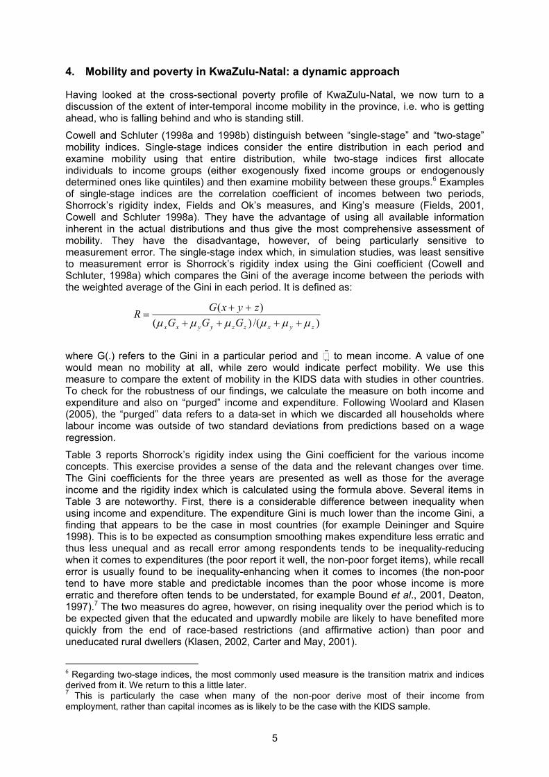
Cowell and Schluter (1998a and 1998b) distinguish between “single-stage” and “two-stage” mobility indices. Single-stage indices consider the entire distribution in each period and examine mobility using that entire distribution, while two-stage indices first allocate individuals to income groups (either exogenously fixed income groups or endogenously determined ones like quintiles) and then examine mobility between these groups.6 Examples of single-stage indices are the correlation coefficient of incomes between two periods, Shorrock’s rigidity index, Fields and Ok’s measures, and King’s measure (Fields, 2001, Cowell and Schluter 1998a). They have the advantage of using all available information inherent in the actual distributions and thus give the most comprehensive assessment of mobility. They have the disadvantage, however, of being particularly sensitive to measurement error. The single-stage index which, in simulation studies, was least sensitive to measurement error is Shorrock’s rigidity index using the Gini coefficient (Cowell and Schluter, 1998a) which compares the Gini of the average income between the periods with the weighted average of the Gini in each period. It is defined as:

)/()(

)(

zyxzzyyxx GGG

zyxGR

µµµµµµ ++++

++=

where G(.) refers to the Gini in a particular period and to mean income. A value of one would mean no mobility at all, while zero would indicate perfect mobility. We use this measure to compare the extent of mobility in the KIDS data with studies in other countries. To check for the robustness of our findings, we calculate the measure on both income and expenditure and also on “purged” income and expenditure. Following Woolard and Klasen (2005), the “purged” data refers to a data-set in which we discarded all households where labour income was outside of two standard deviations from predictions based on a wage regression.

Table 3 reports Shorrock’s rigidity index using the Gini coefficient for the various income concepts. This exercise provides a sense of the data and the relevant changes over time. The Gini coefficients for the three years are presented as well as those for the average income and the rigidity index which is calculated using the formula above. Several items in Table 3 are noteworthy. First, there is a considerable difference between inequality when using income and expenditure. The expenditure Gini is much lower than the income Gini, a finding that appears to be the case in most countries (for example Deininger and Squire 1998). This is to be expected as consumption smoothing makes expenditure less erratic and thus less unequal and as recall error among respondents tends to be inequality-reducing when it comes to expenditures (the poor report it well, the non-poor forget items), while recall error is usually found to be inequality-enhancing when it comes to incomes (the non-poor tend to have more stable and predictable incomes than the poor whose income is more erratic and therefore often tends to be understated, for example Bound et al., 2001, Deaton, 1997).7 The two measures do agree, however, on rising inequality over the period which is to be expected given that the educated and upwardly mobile are likely to have benefited more quickly from the end of race-based restrictions (and affirmative action) than poor and uneducated rural dwellers (Klasen, 2002, Carter and May, 2001).

6 Regarding two-stage indices, the most commonly used measure is the transition matrix and indices derived from it. We return to this a little later. 7 This is particularly the case when many of the non-poor derive most of their income from employment, rather than capital incomes as is likely to be the case with the KIDS sample.

6

Second, the rigidity index for incomes and expenditures indicates a fairly high degree of mobility, when compared with mature industrialised countries where the rigidity index is usually around 0.95 or above for countries such as the US, the United Kingdom, Germany, or Sweden (for example Jarvis and Jenkins, 1998, Eriksson and Pettersson, 2000). It is closer to countries undergoing rapid structural change such as Spain in the 1990s, where it was estimated to be around 0.9 on a comparable basis (Cantó, 2000).

Third, while the “purging”8 affects the Gini coefficients considerably, the rigidity index is scarcely affected. This seems to suggest that any measurement error in the data has a muted impact on the measurement of mobility.

Table 3: Shorrock’s Rigidity Index, KIDS 1993 – 2004

1993 Gini

1998 Gini

2004 Gini

Gini of average income over 3 periods

Rigidity Index

Per capita income

Raw (unpurged) 0.58 0.59 0.68 0.56 0.91

Purged

0.54 0.58 0.63 0.53 0.91

Per capita expenditure

Raw (unpurged) 0.38 0.47 0.59 0.43 0.90

Purged

0.36 0.45 0.58 0.42 0.91

Note: The purged data refer to the income and expenditure data where labour income was outside of two standard deviations from predictions based on a wage regression.

Lastly, despite large differences in inequality between incomes and expenditures, the rigidity index is quite similar. Thus, in the eleven years between 1993 and 2004, incomes and expenditures experienced the same, very high mobility pattern.

While these statistics already tell us quite a lot, we want to unpack mobility beyond this one measure and thus turn to “two-stage” mobility measures, specifically transition matrices, for a more disaggregated look. Analysts concerned with poverty dynamics such as Bane and Elwood (1986) introduced the convention of using transition matrices as an approach to the analysis of dynamic poverty. Subsequent studies making use of panel data such as that undertaken by the Chronic Poverty Research Centre and others have made extensive use of such matrices. As Table 4 shows, such matrices offer a convenient window into poverty transitions between the 1993 and 1998, and 1998 to 2004 waves of data collection. The table is based on a normalised real per capita expenditure measure, defined as total household expenditure divided by the number of resident household members, adjusted to 2000 prices, and divided by the Hoogeveen and Özler per capita poverty line. A normalised expenditure value equal to one, thus, indicates that household per capita expenditures exactly equal the poverty line. A measure of two indicates that household expenditures represent a level of material well-being that is twice the poverty line, and so forth. These values have been grouped into five categories in order to produce the matrix. The table also shows the mean and median change in this poverty score for each of the 1998 and 2004 categories, respectively.

8 The 1993, 1998 and 2004 labour income data was purged by specifying an earnings regression of hourly earnings on gender, location, industry, age, age squared and education and throwing out all observations that are outside two standard deviations from the point estimate of this earnings regression. The earnings regressions have a good fit (adjusted R2 around 0.5) and confirm the usual findings from the human capital literature (regressions available on request). Using this procedure, between four and six per cent of observations were eliminated in each year.

7

Table 4: Transition Matrices using expenditure

a) 1993 to 1998

1998

1993 <0.5 0.5<1 1<1.5 1.5<2 2>

<0.5 50.4 38.3 6.1 3.5 1.7

0.5<1 38.0 36.4 18.7 4.4 2.5

1<1.5 12.4 36.7 24.9 10.2 15.8

1.5<2 9.4 31.1 17.0 16.0 26.4

2> 2.3 8.3 15.8 14.3 59.4

Mean Change -0.4 -0.3 0.0 0.1 1.3

Median Change -0.3 -0.2 0.2 0.3 1.3

b) 1998 to 2004

2004

1998 <0.5 0.5<1 1<1.5 1.5<2 2>

<0.5 40.2 37.4 8.2 6.8 7.3

0.5<1 25.3 33.3 19.0 7.7 14.7

1<1.5 17.9 20.5 26.5 13.9 21.2

1.5<2 2.7 14.7 16.0 16.0 50.7

2> 1.3 6.0 9.4 4.7 78.5

Mean Change -0.3 -0.1 0.0 0.5 2.4

Median Change -0.2 0.1 0.3 0.7 1.6

Both matrices depict substantial and increasing mobility with most cells on the diagonal (in bold and depicting households that remained in the same position between the waves) containing less than 50 percent of the row percentage. The declining fortunes of households in the first wave are also evident from the relatively high values in the cells to the left of the diagonal (in italics) which contain households that fell behind. This situation improves in the second wave in which higher values are to be found to the right of the diagonal. The mean and median changes in the poverty score provide insight into the changes that occurred within the categories. For the 1998-1998 period, the experience of most of those below the poverty threshold was of declining ability to meet household subsistence requirements, while those above the threshold experienced an improvement. Although this pattern is repeated in the 1998-2004 period, the median change in the score is negative only for the poorest category, while the better off categories experienced acceleration in their rate of change.

5. Descriptive statistics

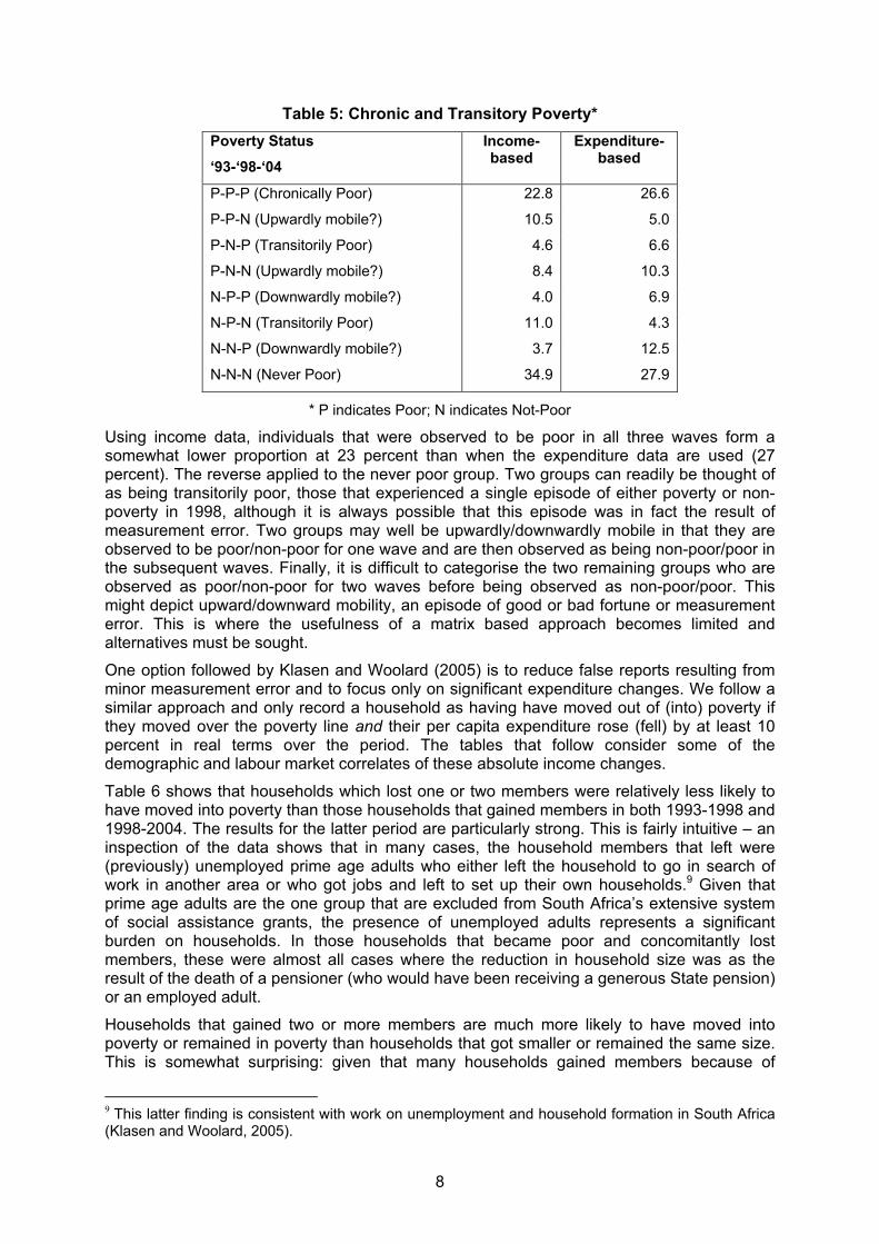
Before turning to more sophisticated analyses, we consider some of the univariate correlates of upward and downward mobility. As a way of depicting poverty transitions that can be derived from the matrices just discussed, Table 5 records the percentage of households observed in all three waves broken down by the number of poverty spells that they have experienced, showing this information for expenditure and for income.

8

Table 5: Chronic and Transitory Poverty*

Poverty Status

‘93-‘98-‘04

Income-based

Expenditure-based

P-P-P (Chronically Poor) 22.8 26.6

P-P-N (Upwardly mobile?) 10.5 5.0

P-N-P (Transitorily Poor) 4.6 6.6

P-N-N (Upwardly mobile?) 8.4 10.3

N-P-P (Downwardly mobile?) 4.0 6.9

N-P-N (Transitorily Poor) 11.0 4.3

N-N-P (Downwardly mobile?) 3.7 12.5

N-N-N (Never Poor) 34.9 27.9

* P indicates Poor; N indicates Not-Poor

Using income data, individuals that were observed to be poor in all three waves form a somewhat lower proportion at 23 percent than when the expenditure data are used (27 percent). The reverse applied to the never poor group. Two groups can readily be thought of as being transitorily poor, those that experienced a single episode of either poverty or non-poverty in 1998, although it is always possible that this episode was in fact the result of measurement error. Two groups may well be upwardly/downwardly mobile in that they are observed to be poor/non-poor for one wave and are then observed as being non-poor/poor in the subsequent waves. Finally, it is difficult to categorise the two remaining groups who are observed as poor/non-poor for two waves before being observed as non-poor/poor. This might depict upward/downward mobility, an episode of good or bad fortune or measurement error. This is where the usefulness of a matrix based approach becomes limited and alternatives must be sought.

One option followed by Klasen and Woolard (2005) is to reduce false reports resulting from minor measurement error and to focus only on significant expenditure changes. We follow a similar approach and only record a household as having have moved out of (into) poverty if they moved over the poverty line and their per capita expenditure rose (fell) by at least 10 percent in real terms over the period. The tables that follow consider some of the demographic and labour market correlates of these absolute income changes.

Table 6 shows that households which lost one or two members were relatively less likely to have moved into poverty than those households that gained members in both 1993-1998 and 1998-2004. The results for the latter period are particularly strong. This is fairly intuitive – an inspection of the data shows that in many cases, the household members that left were (previously) unemployed prime age adults who either left the household to go in search of work in another area or who got jobs and left to set up their own households.9 Given that prime age adults are the one group that are excluded from South Africa’s extensive system of social assistance grants, the presence of unemployed adults represents a significant burden on households. In those households that became poor and concomitantly lost members, these were almost all cases where the reduction in household size was as the result of the death of a pensioner (who would have been receiving a generous State pension) or an employed adult.

Households that gained two or more members are much more likely to have moved into poverty or remained in poverty than households that got smaller or remained the same size. This is somewhat surprising: given that many households gained members because of

9 This latter finding is consistent with work on unemployment and household formation in South Africa (Klasen and Woolard, 2005).

9

births,10 one might have expected that the introduction of the Child Support Grant (for all poor children under the age of seven) after 1998 would have mediated the effect of gaining new household members in the period 1998 to 2004. An inspection of the data suggests, however, that many households that gained members absorbed prime-age adults that were either unemployed or not economically active. This is consistent with other evidence that there has been significant return migration to KwaZulu-Natal of migrant workers that have become unemployed (Case et al., 2005).

Table 6: Poverty status in 1993 & 1998 & 1998 & 2004 by change in household size

a) 1993 to 1998

Change in household size 1993-1998

lost 2 or more persons

Lost 1 person

no change gained 1 person

gained 2 or more persons

Poor in both periods 35.0% 24.8% 20.4% 22.6% 40.9%

Non-Poor in 1993; Poor in 1998 12.8% 19.3% 15.7% 27.8% 25.2%

Poor in 1993; Non-poor in 1998 13.5% 5.5% 6.4% 2.6% 8.7%

Non-poor in both periods 38.7% 55.4% 57.6% 47.0% 25.2%

Total 100% 100% 100% 100% 100%

b) 1998 to 2004

Change in household size 1998-2004

Lost 2 or more persons

Lost 1 person

no change gained 1 person

gained 2 or more persons





Total 100% 100% 100% 100% 100%

Table 7 examines changes in poverty status by the age of the head of the household in 1993. It shows that, for the 1993-1998 period, households headed by a person over the age of 60 were the most likely to have exited poverty in the period 1993 and 1998. Men become eligible for the State Old Age Pension (OAP) at age 65, so many of these household heads “aged into” the OAP during this period. The OAP is not only a secure form of income, but has increased appreciably in real terms since 1993. Households with a head in his/her 40s were the most likely to have fallen into poverty in the first period, largely related to worsening employment prospects (which were partially reversed in the latter period). Among younger people, the picture is somewhat brighter. While poor employment prospects worsened incomes, improved earnings due to higher education and more opportunities for Africans post-apartheid might have off-set this.

10 80% of all households reported at least one new birth between the second and third wave.

10

Table 7: Poverty status in 1993 & 1998 & 1998 & 2004 by age of household head in 1993

a) 1993 to 1998

Age of household head in 1993

<30 30-39 40-49 50-59 60-69 70+

Poor in both periods 19.2% 20.0% 27.3% 29.8% 36.5% 36.3%

Non-Poor in 1998; Poor in 2004 11.5% 14.4% 22.2% 16.9% 19.1% 20.5%

Poor in 1998; Non-poor in 2004 7.7% 4.8% 5.7% 8.4% 13.5% 10.2%

Non-poor in both periods 61.5% 60.8% 44.9% 44.9% 30.9% 32.9%

Total 100% 100% 100% 100% 100% 100%

b) 1998 to 2004

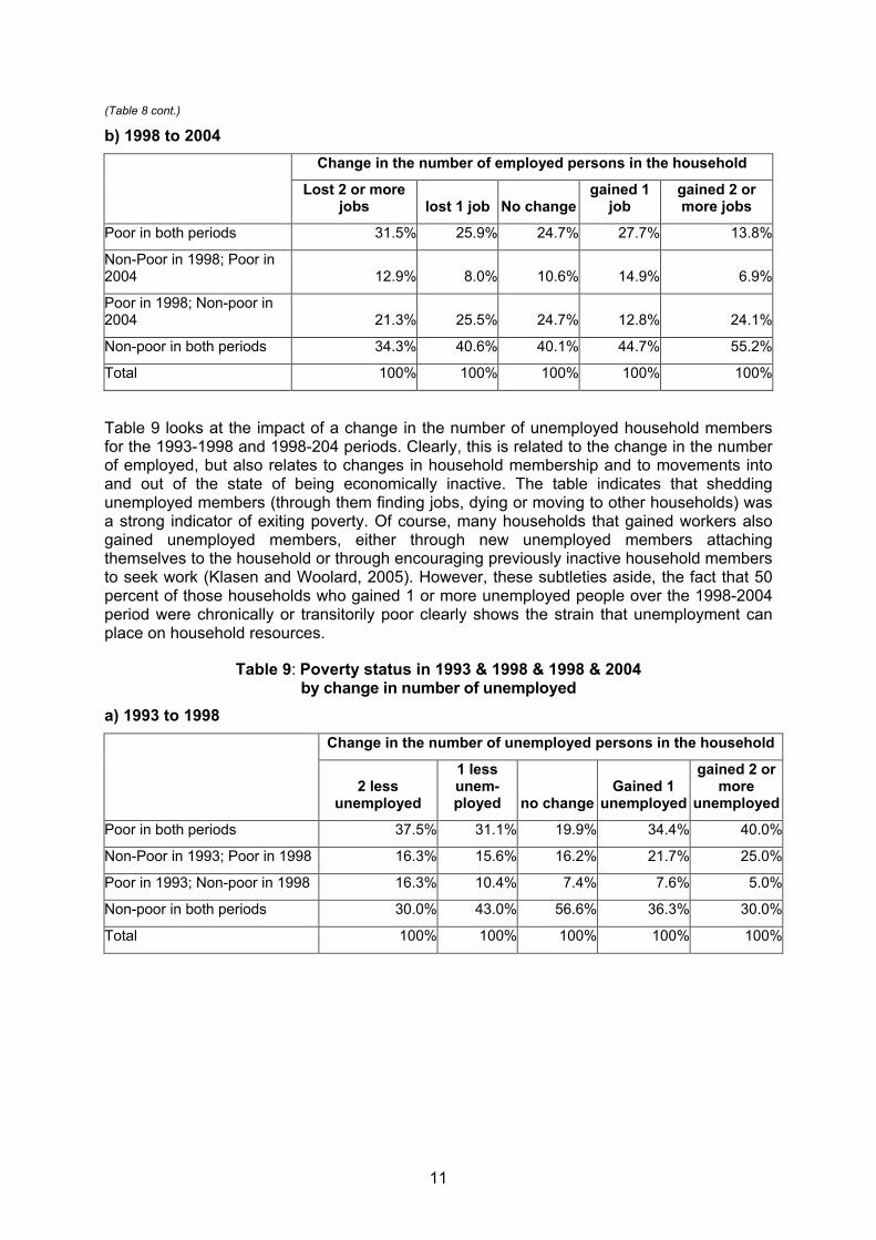
Table 8 focuses directly on the role of employment changes. The trends are surprisingly difficult to discern. For example, the group which lost two or more jobs between the first two waves of the survey was also the most likely to be non-poor in both periods. Not surprisingly, households where additional people obtained employment were the most likely to experience upward mobility. This effect is much stronger for the 1993-1998 period than for the 1998-2004 period: over the latter period, significant percentages of households gained 1 or even 2 workers, yet fell into poverty or remained poor. Many of these households experienced an increase in household size which more than compensated for the additional wage income.

Table 8: Poverty status in 1993 & 1998 & 1998 & 2004 by change in number of employed

a) 1993 to 1998

Change in the (net) number of employed persons in the household

Lost 2 or more jobs Lost 1 job No change

gained 1 job

gained 2 or more jobs





Total 100% 100% 100% 100% 100%

Age of household head in 1998

<30 30-39 40-49 50-59 60-69 70+

Poor in both periods 17.2% 19.8% 28.4% 30.5% 29.7% 32.7%

Non-Poor in 1998; Poor in 2004 10.3% 12.9% 7.4% 8.2% 12.6% 15.7%

Poor in 1998; Non-poor in 2004 37.9% 21.5% 21.0% 18.7% 27.4% 19.8%

Non-poor in both periods 34.5% 45.7% 43.2% 42.6% 30.3% 31.8%

Total 100% 100% 100% 100% 100% 100%

11

(Table 8 cont.)

b) 1998 to 2004

Change in the number of employed persons in the household

Lost 2 or more jobs lost 1 job No change

gained 1 job

gained 2 or more jobs





Total 100% 100% 100% 100% 100%

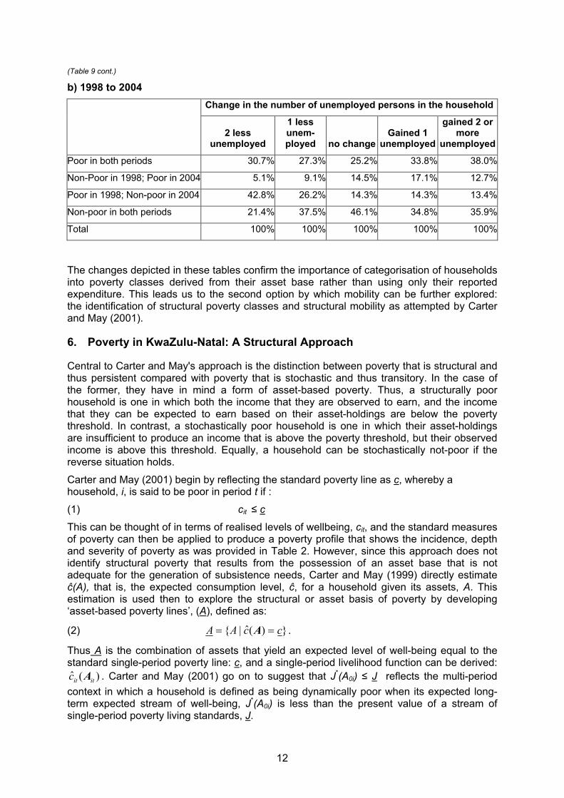
Table 9 looks at the impact of a change in the number of unemployed household members for the 1993-1998 and 1998-204 periods. Clearly, this is related to the change in the number of employed, but also relates to changes in household membership and to movements into and out of the state of being economically inactive. The table indicates that shedding unemployed members (through them finding jobs, dying or moving to other households) was a strong indicator of exiting poverty. Of course, many households that gained workers also gained unemployed members, either through new unemployed members attaching themselves to the household or through encouraging previously inactive household members to seek work (Klasen and Woolard, 2005). However, these subtleties aside, the fact that 50 percent of those households who gained 1 or more unemployed people over the 1998-2004 period were chronically or transitorily poor clearly shows the strain that unemployment can place on household resources.

Table 9: Poverty status in 1993 & 1998 & 1998 & 2004 by change in number of unemployed

a) 1993 to 1998

Change in the number of unemployed persons in the household

2 less unemployed

1 less unem-ployed no change

Gained 1 unemployed

gained 2 or more

unemployed





Total 100% 100% 100% 100% 100%

12

(Table 9 cont.)

b) 1998 to 2004

Change in the number of unemployed persons in the household

2 less unemployed

1 less unem-ployed no change

Gained 1 unemployed

gained 2 or more

unemployed





Total 100% 100% 100% 100% 100%

The changes depicted in these tables confirm the importance of categorisation of households into poverty classes derived from their asset base rather than using only their reported expenditure. This leads us to the second option by which mobility can be further explored: the identification of structural poverty classes and structural mobility as attempted by Carter and May (2001).

6. Poverty in KwaZulu-Natal: A Structural Approach

Central to Carter and May's approach is the distinction between poverty that is structural and thus persistent compared with poverty that is stochastic and thus transitory. In the case of the former, they have in mind a form of asset-based poverty. Thus, a structurally poor household is one in which both the income that they are observed to earn, and the income that they can be expected to earn based on their asset-holdings are below the poverty threshold. In contrast, a stochastically poor household is one in which their asset-holdings are insufficient to produce an income that is above the poverty threshold, but their observed income is above this threshold. Equally, a household can be stochastically not-poor if the reverse situation holds.

Carter and May (2001) begin by reflecting the standard poverty line as c, whereby a household, i, is said to be poor in period t if :

(1) cit ≤ c

This can be thought of in terms of realised levels of wellbeing, cit, and the standard measures of poverty can then be applied to produce a poverty profile that shows the incidence, depth and severity of poverty as was provided in Table 2. However, since this approach does not identify structural poverty that results from the possession of an asset base that is not adequate for the generation of subsistence needs, Carter and May (1999) directly estimate ĉ(A), that is, the expected consumption level, ĉ, for a household given its assets, A. This estimation is used then to explore the structural or asset basis of poverty by developing ‘asset-based poverty lines’, (A), defined as:

(2) })(ˆ|{ ccAA == A .

Thus A is the combination of assets that yield an expected level of well-being equal to the standard single-period poverty line: c, and a single-period livelihood function can be derived:

)(ˆititc A . Carter and May (2001) go on to suggest that J*(A0i) ≤ J reflects the multi-period

context in which a household is defined as being dynamically poor when its expected long-term expected stream of well-being, J*(A0i) is less than the present value of a stream of single-period poverty living standards, J.

13

In terms of Carter and May’s (2001) analysis, households can now be divided between those that are structurally poor (with asset holdings below A), and those that are structurally non-poor (with asset holdings above A) irrespective of the consumption level at which the household is observed at a particular point in time. The structurally poor can in turn be subdivided between those that are caught in a poverty trap below A , unable to accumulate;

and those that are not trapped and are able to accumulate and thus are eventually able to escape from poverty. Finally, at any point in time, households may be stochastically poor (such as a household with asset holding AA >′′′ that that has received a shock, 0<′′′ε , and

is likely to return to its expected livelihood level in time, cAc >′′′ )(ˆ ); or, stochastically non-

poor (such as a household with asset level A ′′ that receives an windfall, 0>′′ε , but that is also likely to return to its expected livelihood level of cAc <′′ )(ˆ ). Stochastic poverty will also

be observed to the extent that measurement errors prevent households from being categorised with certainty.

As Carter and May (1999) explain, there are a number of reasons why )(ˆititc A should depart

from strict linearity or asset additivity and as subsequent analysts have pointed out, measurement errors may have influenced these results. Following on from the methodological suggestion of that paper, subsequently carried out by Carter and May (2001), the precision of the underlying estimation of )(ˆ

ititc A for each household is checked to see

whether the following hypotheses for each year of the data can be rejected:

Household is expected to be poor if reject Hypothesis1: ĉit > c

Household is expected to be non-poor if reject Hypothesis2: ĉit < c.

A household that is observed to be poor, but for whom the hypothesis that they are expected to be poor is rejected, is said be stochastically poor. In some cases these may be households that have suffered an entitlement shock, in others, households in which household expenditure or composition has been incorrectly reported. Similarly, a household that is observed to be non-poor, but for whom the hypothesis that they are expected to be non-poor is rejected is said to be stochastically non-poor. Once again, this result may be due to households that have enjoyed an entitlement windfall or incorrectly reported data.

In order to apply this approach to the three waves of KIDS, the log of the standardised poverty scores was regressed to yield a predicted asset-based score. This livelihood function used the value of productive assets (land, housing and equipment), the mean years of education of resident and non-resident adult members of the household (16 years of age and above), the value of all transfers to the household (government grants, private pension, maintenance payments and remittances) and the interacted value of each of these assets11. The model controlled for the total subsistence needs of the household measured in terms of number of household members weighted by the per capita poverty threshold, and a rural variable derived from population density as reported in the 2001 Population Census12. The results are shown in Table 10.

11/ Carter and May (2001) used the number of educated and uneducated labour units, non-urban/urban dummy variable, productive capital, transfer income, and the number of adult equivalent consumers as explanatory variables in a local regression analysis. 12/ As there currently is no definition of rural and urban in South Africa, enumerator areas with a population density of less than 750 people per square kilometre were classified as being rural.

14

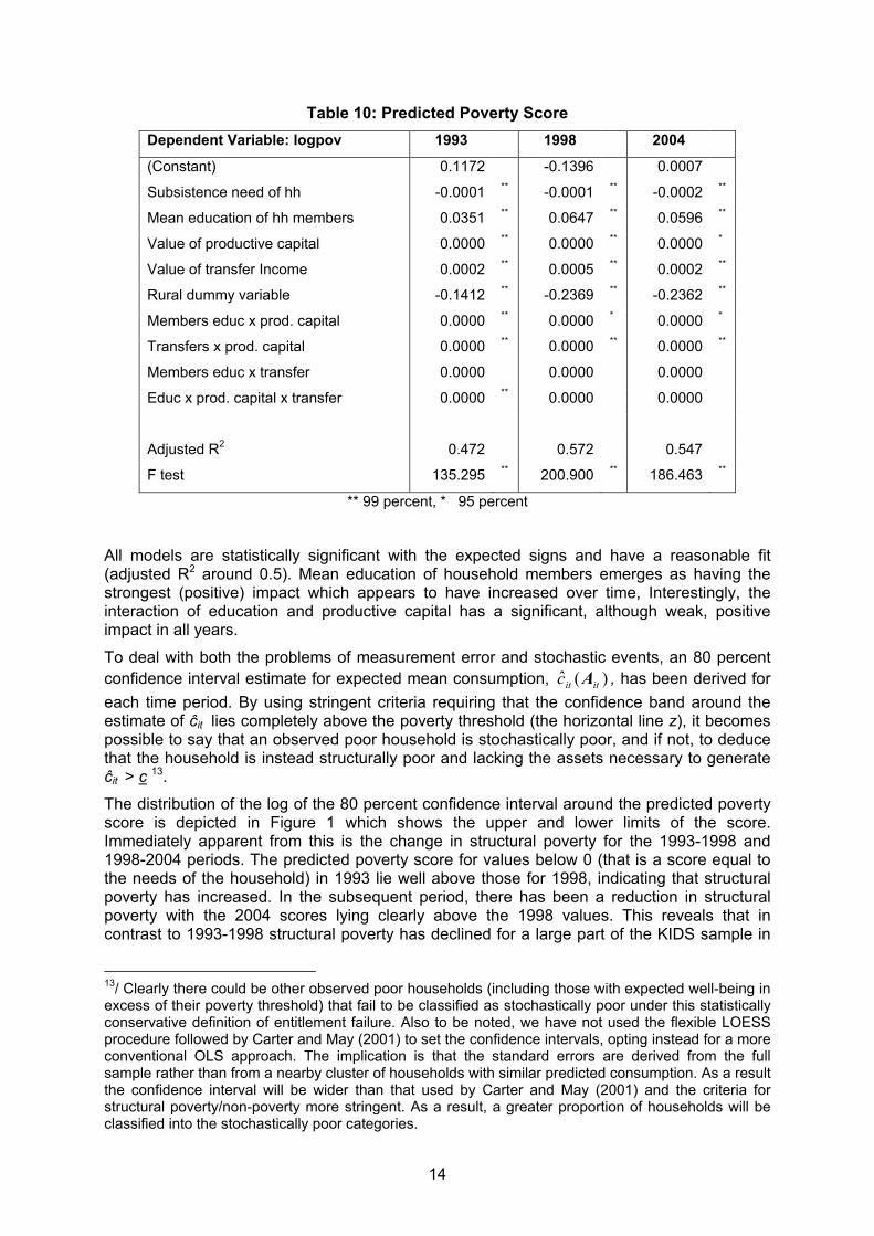
Table 10: Predicted Poverty Score

Dependent Variable: logpov 1993

1998

2004

(Constant) 0.1172 -0.1396 0.0007

Subsistence need of hh -0.0001 ** -0.0001 ** -0.0002 **

Mean education of hh members 0.0351 ** 0.0647 ** 0.0596 **

Value of productive capital 0.0000 ** 0.0000 ** 0.0000 *

Value of transfer Income 0.0002 ** 0.0005 ** 0.0002 **

Rural dummy variable -0.1412 ** -0.2369 ** -0.2362 **

Members educ x prod. capital 0.0000 ** 0.0000 * 0.0000 *

Transfers x prod. capital 0.0000 ** 0.0000 ** 0.0000 **

Members educ x transfer 0.0000 0.0000 0.0000

Educ x prod. capital x transfer 0.0000 ** 0.0000 0.0000

Adjusted R2 0.472 0.572 0.547

F test 135.295 ** 200.900 ** 186.463 **

** 99 percent, * 95 percent

All models are statistically significant with the expected signs and have a reasonable fit (adjusted R2 around 0.5). Mean education of household members emerges as having the strongest (positive) impact which appears to have increased over time, Interestingly, the interaction of education and productive capital has a significant, although weak, positive impact in all years.

To deal with both the problems of measurement error and stochastic events, an 80 percent confidence interval estimate for expected mean consumption, )(ˆ

ititc A , has been derived for

each time period. By using stringent criteria requiring that the confidence band around the estimate of ĉit lies completely above the poverty threshold (the horizontal line z), it becomes possible to say that an observed poor household is stochastically poor, and if not, to deduce that the household is instead structurally poor and lacking the assets necessary to generate ĉit > c

13.

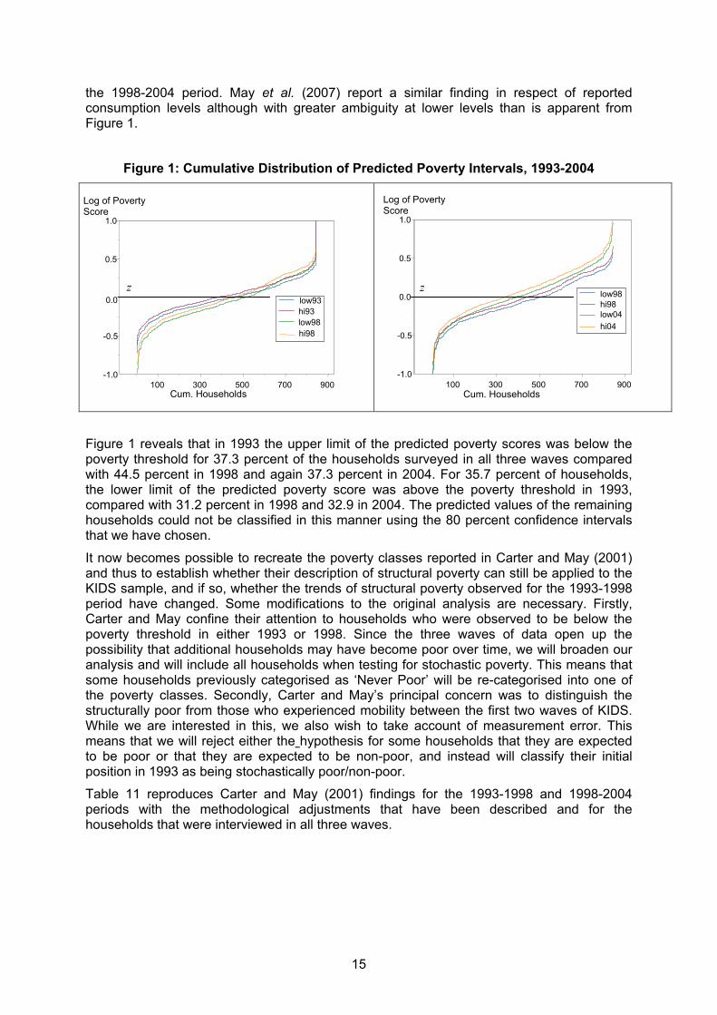
The distribution of the log of the 80 percent confidence interval around the predicted poverty score is depicted in Figure 1 which shows the upper and lower limits of the score. Immediately apparent from this is the change in structural poverty for the 1993-1998 and 1998-2004 periods. The predicted poverty score for values below 0 (that is a score equal to the needs of the household) in 1993 lie well above those for 1998, indicating that structural poverty has increased. In the subsequent period, there has been a reduction in structural poverty with the 2004 scores lying clearly above the 1998 values. This reveals that in contrast to 1993-1998 structural poverty has declined for a large part of the KIDS sample in

13/ Clearly there could be other observed poor households (including those with expected well-being in excess of their poverty threshold) that fail to be classified as stochastically poor under this statistically conservative definition of entitlement failure. Also to be noted, we have not used the flexible LOESS procedure followed by Carter and May (2001) to set the confidence intervals, opting instead for a more conventional OLS approach. The implication is that the standard errors are derived from the full sample rather than from a nearby cluster of households with similar predicted consumption. As a result the confidence interval will be wider than that used by Carter and May (2001) and the criteria for structural poverty/non-poverty more stringent. As a result, a greater proportion of households will be classified into the stochastically poor categories.

15

the 1998-2004 period. May et al. (2007) report a similar finding in respect of reported consumption levels although with greater ambiguity at lower levels than is apparent from Figure 1.

Figure 1: Cumulative Distribution of Predicted Poverty Intervals, 1993-2004

Figure 1 reveals that in 1993 the upper limit of the predicted poverty scores was below the poverty threshold for 37.3 percent of the households surveyed in all three waves compared with 44.5 percent in 1998 and again 37.3 percent in 2004. For 35.7 percent of households, the lower limit of the predicted poverty score was above the poverty threshold in 1993, compared with 31.2 percent in 1998 and 32.9 in 2004. The predicted values of the remaining households could not be classified in this manner using the 80 percent confidence intervals that we have chosen.

It now becomes possible to recreate the poverty classes reported in Carter and May (2001) and thus to establish whether their description of structural poverty can still be applied to the KIDS sample, and if so, whether the trends of structural poverty observed for the 1993-1998 period have changed. Some modifications to the original analysis are necessary. Firstly, Carter and May confine their attention to households who were observed to be below the poverty threshold in either 1993 or 1998. Since the three waves of data open up the possibility that additional households may have become poor over time, we will broaden our analysis and will include all households when testing for stochastic poverty. This means that some households previously categorised as ‘Never Poor’ will be re-categorised into one of the poverty classes. Secondly, Carter and May’s principal concern was to distinguish the structurally poor from those who experienced mobility between the first two waves of KIDS. While we are interested in this, we also wish to take account of measurement error. This means that we will reject either the hypothesis for some households that they are expected to be poor or that they are expected to be non-poor, and instead will classify their initial position in 1993 as being stochastically poor/non-poor.

Table 11 reproduces Carter and May (2001) findings for the 1993-1998 and 1998-2004 periods with the methodological adjustments that have been described and for the households that were interviewed in all three waves.

100 300 500 700 900 -1.0

-0.5

0.0

0.5

1.0

low98 hi98 low04

hi04

100 300 500 700 900 -1.0

-0.5

0.0

0.5

1.0

low93 hi93 low98 hi98

z z

Log of Poverty Score

Cum. Households Cum. Households

Log of Poverty Score

16

Table 11: Decomposing Poverty Transitions in KIDS

a) 1993 - 1998

1998

Poor Non-Poor

Poor

39.9% Chronically Poor, of which:

• 8.9% had experienced dual entitlement failures

• Structurally Poor < 91%

11.0% Got Ahead, of which:

• 52.2% Stochastically poor in 1993

• Structurally mobile < 47.8%

1993

Non-Poor

17.2% Fell Behind, of which:

• 50.7% Stochastically non-poor in 1998

• Structurally downward <49.3%, of which 60.5% had experienced entitlement failures

31.9% Never Poor, of which:

• 7.8% had benefited from dual windfalls

• Structurally never poor < 92.2%

b) 1998-2004

2004

Poor Non-Poor

Poor


• 8.6% had experienced dual entitlement failures





1998

Non-Poor







As with Carter and May (2001), Table 11 allows us to put bounds on the degree of structural and stochastic poverty. For the 1993 to 1998 period, the results are broadly similar to the 2001 paper: to find otherwise would have been a cause for concern. For 8.9 percent of the chronically poor, we can reject the hypothesis that they were structurally poor in both periods, meaning that they are likely to have suffered dual entitlement failures. This defines an upper bound estimate of 91 percent of the chronically poor who are actually structurally poor. Looking at the households that moved from poor to non-poor status between 1993 and 1998, we find that over half (52 percent) received entitlement shocks in 1993 (i.e., we could reject the hypothesis that they were expected to be poor in 1993). The upward mobility of this group can thus be inferred to be a regression to their expected level of livelihood. This places an upper bound of 47.8 percent on the number of the upwardly mobile who escaped poverty though accumulation. Finally, 17.2 percent of households fell behind of which 50.7 percent had suffered a 1998 entitlement failure since we could reject the hypothesis that their expected level of well-being was below their poverty threshold. The other 49.3 of these households are potentially structurally downward. The patterns for the 1998 to 2004 period are similar, although with some promising differences. There is a modest decline in structural

17

poverty, a stronger decline in the percentage of households that fell behind and an increase in the percentage of households that got ahead. The observed patterns of declining poverty discussed earlier appear then to be underpinned by structural improvements to assets and to the returns that can be achieved with these assets.

A final consideration is the poverty dynamics over the entire eleven year period of KIDS. This is shown in Table 12.

Table 12: Decomposing Poverty Transitions in KIDS 1993-2004

2004

Poor Non-Poor

Poor


• 6% had experienced dual entitlement failures





1993

Non-Poor







The patterns remain consistent giving reassurance that the long-term position is one in which upper bounds of approximately 30 percent of the KIDS households were structurally poor, 30 percent structurally never poor, 9 percent structurally upward and 7 percent were structurally downward, half of whom had experienced entitlement failures. The remaining 24 percent can be said to have experienced true forms of transitory poverty. Changes in their poverty status arise from either short-term windfalls or shocks, or from measurement error. As the differences between the periods reveal, for some, these short-term changes become permanent in the long term. Finally, the third wave of data reveal that Carter and May correctly predicted the structural poverty classes for some 75 percent of the structurally poor and structurally not-poor groups, while 66 percent of those observed to be poor in all three waves (conventionally reported as the chronically poor) are found to be structurally poor.

7. Modelling determinants of welfare change: multivariate analysis

Having established that structural poverty can still be usefully applied to the surveyed households in KwaZulu-Natal, and that there may have been a decline in structural poverty for the 1998 to 2004 period, what of the poverty traps that produce this form of long-term poverty and which mediate escape from poverty? Using the first two waves of the KIDS data, Woolard and Klasen (2005) attempted to identify the factors which influenced whether a household improved or worsened its position in the income distribution. They postulate that large initial household size, poor initial education, poor initial asset endowment and poor initial employment access may create poverty traps. We now investigate whether these factors remained as strong between the second and third waves.

The underlying assumption of this model is that household expenditure is a function of household assets (both physical and human) and the economic environment in which these assets can be utilised to generate expenditure. In addition, the well-being of individual household members will depend additionally on the number of people who have to share these assets and the expenditures derived from them.

18

A model of the following form is used:

)RR;K,Kf(=)hhsize

X( iiii

i

i ∆∆∆ ;ln

where Xi = real expenditure of household i

hhsizei = number of (resident) household members in household i

Ki = physical and human assets of household i

Ri = a set of characteristics which summarise the economic and demographic environment in which i operates and thus determines the returns to those assets a household possesses.

The regression was estimated separately for urban and rural African14 households and allowed for further segmentation through the use of dummy variables for the gender of the household head and regional dummies for homeland/non-homeland households. In the urban regression a dummy for the Durban metropolitan area was also included.

Table 13 and 14 present the results for the expenditure change regressions run separately for rural and urban households for the periods 1993-1998, 1998-2004 and 1993-2004. The models all fit very well, with the urban models explaining slightly more of the variation in the data than the rural models.

In all the models, initial expenditure has a negative coefficient, suggesting a strong tendency towards the mean (or convergence of per capita expenditures). Thus the higher per capita expenditure was in the initial period, the more likely the household was to experience a drop in expenditure. This is consistent with the recent findings of Fields et al. (2005) using panel data for Argentina and Venezuela in periods of positive economic growth.

Among the human capital and household composition variables, we find that large initial household size in 1993 reduces per capita expenditure in 1998 in both urban and rural areas. This suggests that larger households had greater difficulty in improving their economic position between 1993 and 1998. This relationship does not, however, continue to hold in the period 1998 to 2004, nor for the period 1993 to 2004 as a whole: these regressions suggest that initial household size is not statistically significant. This may simply indicate that children have grown up and either started to contribute towards household expenses or have left the household. This is consistent with the coefficients on the change in the share of children in the household which are negative, large and highly significant in the urban sample. The change in household size remains very important. In all the regressions an increase in household size between the waves significantly reduces per capita expenditure.

In keeping with the earlier findings of Woolard and Klasen (2005), high initial education and change in education significantly improves upward mobility in both urban and rural areas across all periods. Thus, while improving education is a way out of poverty, those who started with low education will have an additional hurdle to overcome.

14 The regressions were also run for the full sample (i.e. including Indian households) with a dummy variable for African. Not surprisingly, these models fitted less well. These are not shown here as we want to compare our results to those of Woolard and Klasen (2005) who limited their analysis to African households. The regressions for the period 1993-1998 are not identical to those of Woolard and Klasen (2005) as we use per capita expenditure whereas they used adult equivalent income and expenditure.

19

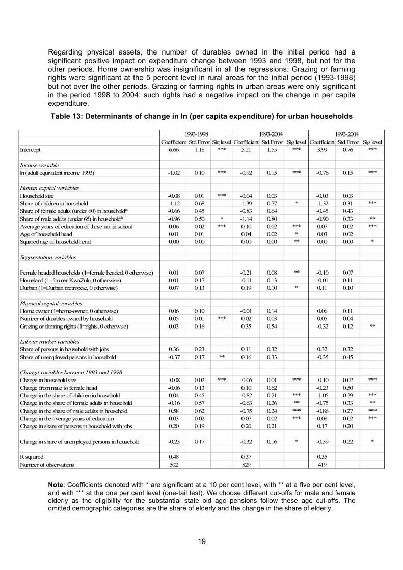
Regarding physical assets, the number of durables owned in the initial period had a significant positive impact on expenditure change between 1993 and 1998, but not for the other periods. Home ownership was insignificant in all the regressions. Grazing or farming rights were significant at the 5 percent level in rural areas for the initial period (1993-1998) but not over the other periods. Grazing or farming rights in urban areas were only significant in the period 1998 to 2004: such rights had a negative impact on the change in per capita expenditure.

Table 13: Determinants of change in ln (per capita expenditure) for urban households

Note: Coefficients denoted with * are significant at a 10 per cent level, with ** at a five per cent level, and with *** at the one per cent level (one-tail test). We choose different cut-offs for male and female elderly as the eligibility for the substantial state old age pensions follow these age cut-offs. The omitted demographic categories are the share of elderly and the change in the share of elderly.

Coefficient Std Error Sig level Coefficient Std Error Sig level Coefficient Std Error Sig level

Intercept 6.66 1.18 *** 5.21 1.55 *** 3.99 0.76 ***

Income variable

ln (adult equivalent income 1993) -1.02 0.10 *** -0.92 0.15 *** -0.76 0.15 ***

Human capital variables

Household size -0.08 0.01 *** -0.04 0.03 -0.03 0.03

Share of children in household -1.12 0.68 -1.39 0.77 * -1.32 0.31 ***

Share of female adults (under 60) in household* -0.66 0.45 -0.83 0.64 -0.45 0.43

Share of male adults (under 65) in household* -0.96 0.50 * -1.14 0.80 -0.90 0.33 **

Average years of education of those not in school 0.06 0.02 *** 0.10 0.02 *** 0.07 0.02 ***

Age of household head 0.01 0.01 0.04 0.02 * 0.03 0.02

Squared age of household head 0.00 0.00 0.00 0.00 ** 0.00 0.00 *

Segmentation variables

Female headed households (1=female headed, 0 otherwise) 0.01 0.07 -0.21 0.08 ** -0.10 0.07

Homeland (1=former KwaZulu, 0 otherwise) 0.01 0.17 -0.11 0.13 -0.01 0.11

Durban (1=Durban metropole, 0 otherwise) 0.07 0.13 0.19 0.10 * 0.11 0.10

Physical capital variables

Home owner (1=home-owner, 0 otherwise) 0.06 0.10 -0.01 0.14 0.06 0.11

Number of durables owned by household 0.05 0.01 *** 0.02 0.03 0.05 0.04

Grazing or farming rights (1=rights, 0 otherwise) 0.03 0.16 0.35 0.54 -0.32 0.12 **

Labour market variables

Share of persons in household with jobs 0.36 0.23 0.11 0.32 0.32 0.32

Share of unemployed persons in household -0.37 0.17 ** 0.16 0.33 -0.35 0.45

Change variables between 1993 and 1998

Change in household size -0.08 0.02 *** -0.06 0.01 *** -0.10 0.02 ***

Change from male to female head -0.06 0.13 0.10 0.62 -0.23 0.50

Change in the share of children in household 0.04 0.45 -0.82 0.21 *** -1.05 0.29 ***

Change in the share of female adults in household -0.16 0.57 -0.63 0.26 ** -0.75 0.33 **

Change in the share of male adults in household 0.58 0.62 -0.75 0.24 *** -0.86 0.27 ***

Change in the average years of education 0.03 0.02 0.07 0.02 *** 0.08 0.02 ***

Change in share of persons in household with jobs 0.20 0.19 0.20 0.21 0.17 0.20

Change in share of unemployed persons in household -0.23 0.17 -0.32 0.16 * -0.39 0.22 *

R squared 0.48 0.37 0.35

Number of observations 502 829 419

1993-1998 1993-2004 1993-2004

20

Table 14: Determinants of change in ln (per capita expenditure) for rural households

Note: Coefficients denoted with * are significant at a 10 per cent level, with ** at a five per cent level, and with *** at the one per cent level (one-tail test). We choose different cut-offs for male and female elderly as the eligibility for the substantial state old age pensions follow these age cut-offs. The omitted demographic categories are the share of elderly and the change in the share of elderly.

The employment variables came in far less strongly than they did in the earlier work of Woolard and Klasen (2005), especially in urban areas. In rural areas, both the initial state variables and the change variables remain important predictors of change in welfare. Rural households with few initially employed members have found it more difficult to improve their level of wellbeing subsequently. This suggests significant segmentation and disadvantage for those from rural households where other household members have little labour market experience (Schoer and Leibbrandt, 2006). In urban areas, however, there is no indication that either the initial state labour market variables nor the change in the number of employed and unemployed has a significant effect on changes in wellbeing. While this is disconcerting, we would venture to suggest that this is consistent with recent work using panel data for

Coefficient Std Error Sig level Coefficient Std Error Sig level Coefficient Std Error Sig level

Intercept 4.37 0.52 *** 4.29 0.60 *** 3.67 0.67 ***

Income variable

ln (adult equivalent income 1993) -0.86 0.05 *** -0.87 0.08 *** -0.72 0.07 ***

Human capital variables

Household size -0.06 0.01 *** -0.02 0.01 * -0.01 0.02

Share of children in household -0.36 0.32 -0.64 0.38 * -0.56 0.41

Share of female adults (under 60) in household* -0.50 0.32 0.30 0.40 0.21 0.38

Share of male adults (under 65) in household* 0.09 0.34 -0.14 0.42 0.05 0.32

Average years of education of those not in school 0.08 0.01 *** 0.08 0.02 *** 0.09 0.01 ***

Age of household head 0.01 0.01 0.00 0.01 0.00 0.02

Squared age of household head 0.00 0.00 0.00 0.00 0.00 0.00

Segmentation variables

Female headed households (1=female headed, 0 otherwise) -0.16 0.05 *** -0.15 0.07 ** -0.08 0.06

Homeland (1=former KwaZulu, 0 otherwise) -0.08 0.09 0.16 0.17 0.14 0.24

Durban (1=Durban metropole, 0 otherwise) (dropped) (dropped) 0.00 *** (dropped)

Physical capital variables

Home owner (1=home-owner, 0 otherwise) 0.05 0.08 0.09 0.14 0.18 0.16

Number of durables owned by household 0.05 0.01 *** 0.04 0.02 * 0.01 0.02

Grazing or farming rights (1=rights, 0 otherwise) 0.13 0.06 ** 0.07 0.08 -0.02 0.08

Labour market variables

Share of persons in household with jobs 0.51 0.14 *** 0.66 0.18 *** 0.39 0.16 **

Share of unemployed persons in household -0.45 0.14 *** -0.01 0.21 -0.42 0.26

Change variables between 1993 and 1998

Change in household size -0.03 0.01 *** -0.04 0.01 *** -0.05 0.01 ***

Change from male to female head -0.17 0.07 ** -0.08 0.13 0.04 0.22

Change in the share of children in household -0.43 0.17 ** -0.46 0.23 * -0.50 0.32

Change in the share of female adults in household 0.16 0.24 -0.30 0.21 -0.28 0.30

Change in the share of male adults in household -0.01 0.19 -0.17 0.23 -0.05 0.30

Change in the average years of education 0.06 0.01 *** 0.06 0.01 *** 0.05 0.02 ***

Change in share of persons in household with jobs 0.49 0.13 *** 0.17 0.10 * 0.49 0.12 ***

Change in share of unemployed persons in household -0.31 0.11 *** -0.12 0.08 -0.32 0.13 **

R squared 0.61 0.52 0.56

Number of observations 163 266 156

1993-1998 1993-2004 1993-2004

21

South Africa (Woolard, 2004; Banerjee et al., 2006) which has demonstrated that there is considerable labour market churn. The KIDS data that we use in this paper spans 11 years with only 3 observations – there is likely to have been very substantial movement into and out of employment between waves that we are unable to observe.

8. Conclusion

In contrast to our earlier work more than a decade has past since a post-apartheid government was elected to power in South Africa. In studies prepared as a part of the 10 year review, despite progress with service delivery, improvement in social policies and improving economic conditions, many analysts acknowledged the persistence of poverty as an issue requiring more direct action. The third wave of the KwaZulu-Natal Income Dynamics Study (KIDS) allows us to take another look at the dynamics of post-apartheid income distribution. Approximately 860 African and Indian households remain in the study in 2004, and using a more carefully thought through poverty threshold we find that the initial increase in poverty rates has been reversed from an increase between 1993 and 1998 from 52 percent to 57 percent, to a decline to 47 percent.

In the previous work, we argued that conventional measures of poverty, including measures of chronic and transitory poverty derived from transition matrices, do not permit us to identify how many households are dynamically poor. Instead we suggested that asset-based approaches which try to identify potential poverty traps would offer better identification of dynamic poverty and its causes. Although we have refined our previous methodologies, we report similar results in which approximately 30 percent of the KIDS households are found to be structurally poor over the eleven year period of the survey, 30 percent structurally never poor, 9 percent structural upward and 7 percent were structurally downward. The remaining 24 percent are in transitory poverty in that the changes in their poverty status arise from either short-term windfalls or shocks, or from measurement error. Seeking an explanation for the persistence of poverty, and in contrast to the previous work of Woolard and Klasen, the only poverty trap for which we find clear evidence when using all three waves is that of low initial education.

Although it is still possible that an eleven-year time period is insufficient to overcome the structural dynamics of apartheid-era poverty production, and to take comfort in the improvements reported in the most recent wave of data collection, the intransigence of a significant level of structural poverty is of concern. The South African government has directed significant resources towards poorer communities and the provision of new forms of support such as the Child Support Grant has placed resources in the hands of many of those in need. However, it is possible that these forms of support will not improve the long term position of those without concomitant improvements in their access to assets. Education suggests itself as an important route out of poverty for many, but it is possible that opportunities may be found to improve other assets of the structurally poor including their land, their access to finance and their access to productive capital.

22

References

Adato, M., Carter, M. R. and May, J. (2006) Exploring poverty traps and social exclusion in South Africa using qualitative and quantitative data, Journal of Development Studies 42(2) 226-247.

Agüero, J., Carter, M. R. and May, J. (forthcoming) Poverty and inequality in the first decade of South Africa’s democracy: what can be learnt from panel data from KwaZulu-Natal? Journal of Southern African Economies.

Bane, M. J. and Ellwood, D. T. (1986) Slipping into and out of poverty, the dynamics of spells. Journal of Human Resources 21(1): 1-23.

Banerjee, A., Galiani, S., Levinsohn, J. and Woolard, I. (2006) Why Has Unemployment Risen in the New South Africa? CID Working Paper Number 134.

Bound, J., Brown, C. H. and Methiowetz, N. (2001) Measurement Error in Survey Data, Handbook of Econometrics, Vol. 5, pp. 3705-3843, Amsterdam: North-Holland.

Cantó, O. (2000) Income mobility in Spain: how much is there? Review of Income and Wealth 46, 85-102.

Carter, M. and May, J. (2001) One kind of freedom. World Development, 29:1987–2006.

Carter, M. R. and May, J. (1999) Poverty, Livelihood and Class in Rural South Africa. World Development 27(1): 1-20.

Case, A., Hosegood, V. and Lund, F. (2005) The reach and impact of child support grants: Evidence from KwaZulu-Natal. Development Studies 22(4): 467-482.

Cowell, F. and Schluter, C. (1998a) Income Mobility: A Robust Approach, STICERD Discussion Paper No. DARP 37, LSE, London.

Cowell, F. and Schluter, C. (1998b) Measuring Income Mobility with Dirty Data, CASE/16, LSE, London.

Deaton, A. (1997) The Analysis of Household Surveys, Johns Hopkins University Press, Baltimore.

Deininger, K. and Squire, L. (1998) New ways of looking at old issues: inequality and growth. Journal of Development Economics 57(2): 257-285.

Eriksson, I. and Pettersson, T. (2000) Income Distribution and Income Mobility- Recent Trends in Sweden. In: Hauser, R. and Becker, I. (eds.) The Personal Distribution of Income in an Historical Perspective, Springer, Berlin, pp.158-176.

Fields, G., Sanchez Puerta, M., Hernandez, R. and Freije, S. (2005) Earnings mobility in Argentina, Mexico and Venezuela: testing the divergence of earnings and the symmetry of mobility hypotheses. Unpublished mimeo.

Fields, G. S. (2001) Distribution and Development: A New Look at the Developing World, MIT Press, Cambridge.

Foster, J., Greer, J. and Thorbecke, E. (1984) A class of decomposable poverty measures, Econometrica 52: 761-765.

Hoogeveen, J. G. and Özler, B. (2005) Not separate, not equal: poverty and inequality in post-apartheid South Africa William Davidson Institute Working Paper No. 739. Ann Arbor: University of Michigan.

Hulme, D. and Shepherd, A. (2003) Conceptualizing chronic poverty. World Development, 21(3): 403-425.

Jarvis, S. and Jenkins, S. P. (1998) How much income mobility is there in Britain? Economic Journal 108, 428-443.

23

Klasen, S. (2002) Social, economic, and environmental limits for the newly enfranchised in South Africa? Economic Development and Cultural Change 50, 607-642.

May, J., Aguero, J., Carter, M. R. and Timæus, I. R. (Forthcoming) The KwaZulu-Natal Income Dynamics Study (KIDS) 3rd wave: methods, first findings and an agenda for future research, Development Southern Africa.

May, J., Carter, M., Haddad, L. and Malluccio, J. (2000) Kwa-Zulu Natal Income Dynamics Study (KIDS) 1993-1998: a longitudinal household data set for Southern African policy analysis, Development Southern Africa 17(4): 567-581.

Meth, C. (2006) What was the poverty headcount in 2004? A critique of the latest offering from van der Berg et al., unpublished research paper, School of Development Studies, University of KwaZulu-Natal.

Meth, C. and Dias, R. (2004) Increases in poverty in South Africa, 1999-2002, Development Southern Africa 21(1), 59-86.

Schoer, V. and Leibbrandt, M. (2006) Determinants of job search strategies: evidence from the Khayelitsha/Mitchell’s Plain Survey. South African Journal of Economics 74(4): 702-724.

Simkins, C. (2004) What happened to the distribution of income in South Africa between 1995 and 2001?, downloaded from http://www.sarpn.org.za/documents/d0001062/index.php on 01 March, 2005.

Stats SA (2002) Earning and spending in South Africa. Selected findings and comparisons from the income and expenditure surveys of October 1995 and October 2000. Pretoria: Statistics South Africa

Van der Berg, S., Burger, R., Louw, M. and Yu, D. (2005) Trends in poverty and inequality since the political transition. Stellenbosch Economic Working Papers, 1/2005, University of Stellenbosch, downloaded from http://www.ber.sun.ac.za/downloads/2005/working _papers/WP-01-2005.pdf on 17 January, 2006.

Van der Berg, S. and Louw, M. (2003) Changing patterns of South African income distribution: towards time series estimates of distribution and poverty, paper to the Conference of the Economic Society of South Africa, Stellenbosch, 17-19 September, 2003.

Woolard, I. (2004) Are the Unemployed a Homogenous Group? Evidence from Panel Data in KwaZulu-Natal. Labour Markets and Social Frontiers 6:1-3.

Woolard, I. and Klasen S. (2005) Determinants of income mobility and household poverty dynamics in South Africa. Journal of Development Studies 41: 865-897.

Documents

Poverty traps and structural poverty in South Africa ...Poverty traps and structural poverty in South Africa. Reassessing the evidence from KwaZulu-Natal Julian May and Ingrid Woolard