Consumption and Income Poverty over the Business … · Consumption and Income Poverty over the Business Cycle ... off-the-books income, inter-family ... exploit both regional and

NBER WORKING PAPER SERIES

CONSUMPTION AND INCOME POVERTY OVER THE BUSINESS CYCLE

Bruce D. MeyerJames X. Sullivan

Working Paper 16751http://www.nber.org/papers/w16751

NATIONAL BUREAU OF ECONOMIC RESEARCH1050 Massachusetts Avenue

Cambridge, MA 02138January 2011

We have benefited from the comments of participants at the IZA/OECD Workshop “Economic Crisis,Rising Unemployment and Policy Responses: What Does It Mean for the Income Distribution?” Theviews expressed herein are those of the authors and do not necessarily reflect the views of the NationalBureau of Economic Research.

NBER working papers are circulated for discussion and comment purposes. They have not been peer-reviewed or been subject to the review by the NBER Board of Directors that accompanies officialNBER publications.

© 2011 by Bruce D. Meyer and James X. Sullivan. All rights reserved. Short sections of text, not toexceed two paragraphs, may be quoted without explicit permission provided that full credit, including© notice, is given to the source.

Consumption and Income Poverty over the Business CycleBruce D. Meyer and James X. SullivanNBER Working Paper No. 16751January 2011JEL No. D6,E3,I3

ABSTRACT

We examine the relationship between the business cycle and poverty for the period from 1960 to 2008using income data from the Current Population Survey and consumption data from the Consumer ExpenditureSurvey. This new evidence on the relationship between macroeconomic conditions and poverty isof particular interest given recent changes in anti-poverty policies that have placed greater emphasison participation in the labor market and in-kind transfers. We look beyond official poverty, examiningalternative income poverty and consumption poverty, which have conceptual and empirical advantagesas measures of the well-being of the poor. We find that both income and consumption poverty aresensitive to macroeconomic conditions. A one percentage point increase in unemployment is associatedwith an increase in the after-tax income poverty rate of 0.9 to 1.1 percentage points in the long-run,and an increase in the consumption poverty rate of 0.3 to 1.2 percentage points in the long-run. Theevidence on whether income is more responsive to the business cycle than consumption is mixed.Income poverty does appear to be more responsive using national level variation, but consumptionpoverty is often more responsive to unemployment when using regional variation. Low percentilesof both income and consumption are sensitive to macroeconomic conditions, and in most cases lowpercentiles of income appear to be more responsive than low percentiles of consumption.

Bruce D. MeyerHarris School of Public PolicyUniversity of Chicago1155 E. 60th StreetChicago, IL 60637and [email protected]

James X. SullivanDepartment of Economics447 Flanner HallUniversity of Notre DameNotre Dame, IN [email protected]

1

1. Introduction

There are two standard sets of tools that have been used to reduce poverty: programs

that directly target poor populations, and policies that alleviate poverty indirectly through

economic growth that benefits the worst off. There is a consensus that the latter set of policies

has greater potential impact.1 In her essay on fighting poverty Blank (2000) concludes that “a

strong macroeconomy matters more than anything else.” However, in some periods the

relationship between growth and poverty appears weak. There is also disagreement on the

link between specific policies and the macroeconomy. We reexamine the relationship

between the macroeconomy and poverty. We do this in part because past work has found a

changing relationship between poverty and measures of the macroeconomy. Past work has

emphasized that the relationship between official poverty and unemployment is very strong in

some decades, but weak in others. There is even greater concern that the relationship may be

different in recent years than in the past because our safety net has undergone a dramatic

transformation. Policies such as welfare reform, EITC expansions, expanded childcare, and

restrictions on use of food stamps by the able bodied have pushed many low income families

to be more reliant on employment. We expect that the effects of macroeconomic conditions

on poverty will be greater when the poor are more closely attached to the labor market. On

the other hand, the argument that economic growth helps those at the bottom may also be less

evident during times, such as recent decades, when growth is accompanied by a rise in income

inequality. In addition there are a number of groups that are less likely to be affected by

macroeconomic fluctuations including those on disability or retirement benefits, both of

which have grown recently.

Our analyses will consider several indicators of the well-being of those at the bottom

of the distribution. Looking beyond official income poverty measures to improved, broader

measures of well-being is important for several reasons. Official pre-tax income poverty has

been widely criticized as poorly measuring the well-being of the worst off. The official

measure fails to capture all the resources available to the family including in-kind transfers

and tax credits that have been key tools in the anti-poverty efforts of the last decades. Other

1 For example, see Blank and Blinder (1986), Blank (2000), Haveman and Schwabish, (2000).

2

flaws include an unattractive adjustment for family size and changes in the real value of the

poverty thresholds over time due to biases in the CPI (Citro and Michael, 1995; Meyer and

Sullivan, 2009).

More importantly, changes in consumption may provide a better measure of the effect

of the economy on the well-being of the worst off than changes in income. Even when

income changes, consumption may vary little if transfers from extended family members, in-

kind government transfers, or access to savings or credit shield a families’ living standards

from transitory changes in income (Cutler and Katz, 1991; Slesnick, 1993, 2001; Meyer and

Sullivan, 2008, 2009). If the importance of factors such as extended families and access to

credit changes over time, the effect of the economy on well-being will likely change. Because

consumption reflects home and car ownership, which provide a flow of consumption services

to their owners even though not captured by income, consumption may provide a better

picture of well-being if ownership rates differ across groups or over time.

The consumption and income data available in the U.S. are both subject to error, but

there is evidence that consumption is reported better than income for those near the bottom of

the distribution. For example, income is often far below consumption for those with few

resources, even for those with little or no assets or debts (Meyer and Sullivan 2003, 2007).

Income measurement issues may be particularly important for this study because many of the

types of income that may be more important in recessions seem to be poorly measured in

household surveys. For example, in bad economic times, off-the-books income, inter-family

transfers, and government transfers are likely to be more prevalent. Each of these sources is

not well reported in household surveys (Edin and Lein, 1997; Meyer, Mok, and Sullivan,

2009). Our analyses will shed light on whether consumption poverty is less sensitive to

macroeconomic conditions because of the wide variety of ways in which households can

smooth their consumption and because mis-reporting of income is likely to be more cyclically

sensitive than mis-reporting of consumption.

In addition to alternative poverty rates, we consider how the macroeconomy affects

low percentiles of the income and consumption distributions. These analyses provide a better

picture of the sensitivity of the bottom of the distribution to economic conditions than

focusing exclusively on a poverty rate, which is the cumulative distribution function of

resources evaluated at a single point.

3

We find that both income and consumption poverty are sensitive to macroeconomic

conditions. The evidence on whether income is more responsive to the business cycle than

consumption is mixed. Income poverty does appear to be more responsive using national

level variation, but consumption poverty is often more responsive to unemployment when

using regional variation. Our results suggest that, for the period from 1981 to 2008, a 1

percentage point increase in unemployment is associated with an increase in the after-tax

income poverty rate of 0.9 to 1.1 percentage points, and an increase in the consumption

poverty rate of 0.3 to 1.2 percentage points. Results for the 2000s indicate that after-tax

income poverty is responsive to changes in the national unemployment rate, although the

point estimates are smaller than for the 1990s.

The evidence for low percentiles is consistent with that for poverty. Low percentiles

of both income and consumption are sensitive to macroeconomic conditions, and in most

cases low percentiles of income appear to be more responsive than low percentiles of

consumption. Across several low income percentiles, we find that a 1 percentage point

increase in unemployment is associated with a decline in these percentiles ranging from 4 to

10 percent. For low percentiles of consumption this range is from 0 to 7 percent.

This paper advances knowledge in a number of respects. First, we look beyond

official poverty, examining alternative income poverty and consumption poverty. Second, we

update the relationship between macroeconomic conditions and poverty through 2008. Given

the sensitivity to time period found in past work, and recent policy changes, recent years are

of special interest. Third, we examine low percentiles of income and consumption to provide

a more complete picture of how macroeconomic conditions affect the worst off. Finally, we

exploit both regional and national variation in economic conditions.

There are a number of limitations to any analysis of this kind. The relationship

between economic conditions and poverty will depend on how government policy responds to

a recession. We necessarily estimate the combined effect of macroeconomic conditions and

any policy adjustments engendered by those conditions. Also, business cycles vary

considerably in the extent to which they affect different industries, demographic groups, or

regions. Thus, the relationship between macroeconomic conditions and poverty will differ

across cycles. The unique nature of each business cycle makes it difficult to draw general

conclusions about the impact of changes in macroeconomic conditions. Moreover, it is

4

difficult to estimate precisely how the response of poverty to the business cycle changes over

time given the short time series for these subperiods. Our own robustness analyses, as well as

comparisons of our results to others in the literature, demonstrate variation in estimates across

equally plausible specifications for narrow time periods, such as a single decade.

In the following section we briefly summarize the key findings from previous studies

of the effect of macroeconomic conditions on poverty. In Section 3 we describe the data used

to construct alternative income and consumption measures of poverty and the methods used to

examine how the macroeconomy is related to these outcomes. We present our results in

Section 4. In Section 5 we briefly simulate poverty rates for the current recession and we

offer conclusions in Section 6.

2. Previous Research on Poverty and Macroeconomic Conditions

A long series of papers have examined the relationship between macroeconomic

conditions and poverty.2 The consensus from this literature is that the relationship between

national unemployment and official poverty is strong, but the magnitude of the effect is

sensitive to the years examined.3 For example, using data from 1959-1983, Blank and Blinder

(1986) find that a one percentage point rise in unemployment results in a 1.1 percentage point

increase in poverty. Comparable estimates from Cutler and Katz (1991), whose sample period

covers 1959-1989, indicate that a one point rise in the unemployment rate raises poverty by

0.43 to 0.69 points. These and other papers conclude that the effect of inflation on poverty is

much more modest than that of unemployment.4

The literature has also emphasized that the relationship between macroeconomic

conditions and poverty has changed over time. Early studies documented a strong

relationship for the 1960s. However, there is evidence that this relationship weakened in the

1970s and particularly the 1980s (Blank, 1993). During the economic expansion from 1983 to

2 See Haveman and Schwabish (2000) for a brief review of this literature. 3 Studies using regional or state variation in poverty and macroeconomic conditions have found similar evidence (Blank and Card, 1993; Tobin, 1994; Freeman, 2001; Gundersen and Ziliak, 2004; Hoynes, Page, and Stevens, 2006). 4 Several papers have considered the effect that government transfer spending has on poverty (Gottschalk and Danziger, 1984; Blank and Blinder, 1986; Haveman and Schwabish, 2000; Blank 2009). These studies typically find that greater transfer spending is associated with reduced poverty, but the estimates are imprecise.

5

1989, real GDP grew by 27 percent, unemployment fell by 45 percent, but poverty fell a

modest 16 percent. More recent studies have shown the relationship between unemployment

and poverty to be stronger in the 1990s than in the 1980s but still weaker than earlier years

(Blank, 2000; Haveman and Schwabish, 2000).

A number of studies have documented how the relationship between macroeconomic

conditions and poverty differs across demographic groups. Recent examples include Blank

(2000, 2009) and Gundersen and Ziliak (2004). Blank (2000, 2009) finds that poverty is

particularly responsive to unemployment for groups that have high exposure to public

assistance: single mother families and black families. In the earlier paper, she finds for both

of these groups that the relationship is stronger in the 1990s than in any earlier decade.

Our paper contributes to the existing literature in several important ways. First, this

literature has focused, almost exclusively, on officially measured poverty.5 We consider

alternative poverty measures that address known criticisms in the official measure. In

addition to broader measures of income poverty, we examine consumption poverty, which is

arguably a better measure of the well-being of the poor. As far as we know, we are the first to

look at the relationship between macroeconomic conditions and consumption poverty.

Second, we update past work by examining the relationship between macroeconomic

conditions and poverty through 2008. This recent evidence is particularly interesting given

the flurry of anti-poverty policies over the past two decades that have placed greater emphasis

on participation in the labor market and in-kind transfers. Third, in addition to poverty

measures, we will look at low percentiles of the distributions of income and consumption to

provide a more complete picture of how the bottom of the distribution responds to the

business cycle. Finally, we exploit both regional and national variation in economic

conditions. This additional source of variation allows us to estimate more precisely how

economic conditions are related to the well-being of the worst-off. In addition, we can

estimate models with year fixed effects, which control for aggregate changes that have similar

effects on poverty or low percentiles in all regions, such as changes in federal tax and transfer

policies.

5 One exception is Gundersen and Ziliak (2004), who look at an after-tax income poverty measure.

6

3. Data and Methods

Our analyses of the relationship between macroeconomic conditions and the well-

being of the worst off relies on official statistics on unemployment and poverty, as well as

alternative poverty measures and percentiles of the income and consumption distribution that

we calculate using nationally representative survey data. The income data come from the

ASEC/ADF Supplement to the Current Population Survey (CPS) and the consumption data

come from the Interview component of the Consumer Expenditure (CE) Survey.

The CPS is the source for many official income statistics including poverty rates.

Respondents to the CPS report information on a number of different sources of money

income. In addition, the survey collects information on some noncash benefits such as food

stamps, housing subsidies, and public health insurance. To calculate alternative income

poverty measures and percentiles of the income distribution, we use the 1964-2009 CPS

surveys, which provide data on income for the previous calendar year. In the analyses that

follow, we consider three different measures of income: pre-tax money income, after-tax

money income, and after-tax money income plus noncash benefits. Pre-tax money income is

the measure used in official poverty statistics. To calculate after-tax money income we add

the value of tax credits such as the EITC, and subtract state and federal income taxes and

payroll taxes, as explained in the Data Appendix. Our measure of after-tax money income

plus noncash benefits adds to after-tax money income the cash value of food stamps, and

imputed values for housing and school lunch subsidies, and the imputed value of Medicaid

and Medicare coverage. For more details, see the Data Appendix.

The CE Survey is the most comprehensive source of spending data for the U.S. To

calculate the consumption poverty rate and percentiles of the consumption distribution, we use

data from the CE Survey for the years 1960-1961, 1972-1973, 1980-1981 and 1984-2008.

The 1960-1961 surveys provide data on annual expenditures collected in a single interview,

while the 1972-1973 surveys provide data on annualized expenditures collected from

quarterly interviews. Since 1980, quarterly expenditures have been provided. To obtain

annual measures we multiply these quarterly measures by four. We do not use the data from

the fourth quarter of 1981 through the fourth quarter of 1983 because the surveys for these

quarters only include respondents from urban areas. We group the data for the 1960-1961

7

period because the data are only representative of the full population when the samples from

these two years are combined.

Our measure of consumption includes both durable and nondurable goods. To convert

reported expenditures into a measure of consumption, we make a number of adjustments.

First, we convert vehicle spending to a service flow equivalent. Instead of including the full

purchase price of a vehicle, we calculate a flow that reflects the value that a consumer

receives from owning a car during the period that is a function of a depreciation rate and the

current market value of the vehicle (see the Data Appendix). Second, to convert housing

expenditures to housing consumption for homeowners, we exclude mortgage interest

payments, property tax payments, and spending on insurance, maintenance and repairs, and

add the reported rental equivalent of the home. Third, for respondents living in government or

subsidized housing, we impute a rental value using detailed housing characteristics available

in the survey. Finally, we exclude spending that is better interpreted as an investment such as

spending on education and health care, and outlays for retirement including pensions and

social security.6 For more details, see the Data Appendix.

Our measure reflects family consumption of goods and services, but does not capture

other important components of consumption such as home production of food, food

preparation, and home repair and maintenance. It is important to note, however, that these

components are also missed in an income measure.

Our poverty rates measure the fraction of all individuals who live in families with

resources that are below a poverty threshold. Resources are measured at the family level. To

adjust for differences in family size and composition we scale all measures using an NAS

recommended equivalence scale (Citro and Michael, 1995): (A + 0.7K)0.7, where A is the

number of adults in the family and K is the number of children. See Meyer and Sullivan

(2009) for a discussion of the importance of equivalence scales for poverty measurement. For

each scale-adjusted measure, the poverty threshold in 1980 is specified as the point in the

distribution in 1980 such that the poverty rate for that measure is equal to that of the official

poverty rate in 1980 (13.0 percent). To obtain thresholds for other years, these thresholds are

6 We also exclude spending on individuals or entities outside the family, such as charitable contributions and spending on gifts to non-family members. This category is very small relative to total consumption.

8

adjusted for inflation using the CPI-U-RS.7 Anchoring our alternative poverty measures to

the official poverty rate in 1980 facilitates comparisons across measures, allowing us to

examine the same point of the distribution initially so that different measures do not diverge

simply because of differential changes at different points in the distribution. In addition to

calculating a national level poverty rate for each year, we also calculate separate poverty rates

for four geographic regions: the Northeast, Midwest, South and West. These are the

narrowest geographic regions identifiable in CE Survey data for all years.

In addition to poverty rates, we also examine the relationship between macroeconomic

conditions and low percentiles of the distribution of consumption or after-tax income. The

percentiles of the distribution are determined in each year after adjusting for differences in

family size using the NAS-recommended equivalence scale.

We focus on two annual measures of macroeconomic conditions. The first is the

national unemployment rate for the U.S. civilian population age 16 and older. We also

examine regional unemployment data, for each of the four regions that are identifiable in both

the CPS and the CE Survey.8 Data on the national unemployment rate are available for our

entire sample period, but data on the regional unemployment rate are only available for the

years from 1976 through 2008.9

The national unemployment rate and our main outcome variables are shown for

various years in Table 1. Over most periods, the unemployment rate and the poverty rate

move in the same direction regardless of how poverty is measured. However, in some cases,

the reverse is true. For example, the unemployment rate rises by 1.5 percentage points

between 1972 and 1980, while the after-tax income and consumption poverty rates both fall

by 1.2 percentage points. Changes in the 10th percentiles of income and consumption are

similar, although the 10th percentile of income is a bit more volatile, and the two measures

diverge between 2000 and 2008.

7 The official poverty thresholds are adjusted for inflation using the CPI-U. The CPI-U-RS corrects for many, but not all, of the biases in the CPI-U. See Meyer and Sullivan (2009) for more details. 8 We also estimate specifications using GDP and median family income as a measure of macroeconomic conditions. We discuss these results briefly in Section 5. 9 The unemployment data are available at the Bureau of Labor Statistics (www.bls.gov/data/#unemployment).

9

To determine how the poverty rate and percentiles are related to either national or

regional variation in macroeconomic conditions we estimate several different models. At the

national level, we estimate

∑−

=− +++++++=

1

1,1,,1,,1111111 ]*[

D

dttddtddtttt tdecadedecadetInflationyUy εκδτπλβα (1)

where yt represents a national poverty rate or a percentile of income or consumption in year t

and Ut is the national unemployment rate for year t. We include a lagged value of the

dependent variable since poverty rates and percentiles are slow to change. Inflationt, which is

the change in the CPI-U-RS between years t and t-1, is included because past work has

hypothesized that it might reduce the real incomes of the poor, such as those with unindexed

pensions. Finally, we include a linear time trend, indicator variables for the D decades in the

sample period, and the interaction of the time trend and the decade indicators. Because much

of the previous literature has focused on how the relationship between macroeconomic

conditions and poverty has changed over time we also estimate models that allow the

relationship to differ by decade:

∑

∑−

=

−=

+++

++++=

1

1,2,,2,,2

22121

,,22

]*[

]*[

D

dttddtdd

tt

D

dttddt

tdecadedecade

tInflationyUdecadey

εκδ

τπλβα (2)

For any given year, both the unemployment rate and the poverty rate will differ

considerably across regions in the U.S. This additional source of variation allows us to

estimate more precisely how economic conditions are related to the well-being of the worst-

off. Another important advantage of examining this relationship regionally is that it allows us

to include year fixed effects, which control for any aggregate changes that have similar effects

on poverty or low percentiles in all regions, such as changes in federal tax and transfer

policies. Specifically, we estimate a model that includes region (Rj) and year (γt) fixed

effects:

jttjjtjtjt RyUy ,31333 εγλβα +++++= − . (3)

Alternatively, to consider whether the relationship between regional economic conditions and

poverty has changed over time we estimate models that allow the relationship to differ by

decade:

10

∑ ∑=

−

=− ++++++=

D

d

D

djttddtjjtjttddjt decadeRyUdecadey

1

1

1,4,,414,,44 ][]*[ εδγλβα . (4)

4. Results

To examine the bivariate relationship between the macroeconomy and the well-being

of the worst off, we construct scatter plots of annual unemployment and the official poverty

rate for the years 1960 through 2008. These plots are shown for four separate time periods in

Figure 1. The results for the 1960s show the strong relationship between unemployment and

official poverty for this decade that has been emphasized in many previous studies. Both

unemployment and poverty fell sharply during this decade. This positive relationship is much

less evident in the 1970s and 1980s, but is more noticeable again in the 1990s and 2000s.

Figure 2 provides similar plots for after-tax income and consumption poverty. The

patterns for after-tax income poverty are fairly similar to those for official income poverty.

For the 1960s, we again see a strong positive relationship between poverty and

unemployment. The pattern is somewhat different for the 1970s, however, when

unemployment and after-tax income poverty are inversely related for part of the decade. For

the period from 1980 to 2008, we also show the relationship between consumption poverty

and unemployment.10 These scatter plots indicate a positive relationship between

consumption poverty and unemployment that is fairly similar to that for after-tax income

poverty.

Table 2 presents estimates of equations 1 and 2 for three different measures of income

poverty: official poverty, after-tax income poverty, and after-tax income plus noncash benefits

poverty. We provide estimates for different sample periods so that we can compare estimates

across outcomes for the same periods. Because all specifications include a lag of the

dependent variable on the right hand side, we also report in brackets the long run derivatives,

which are calculated as β/(1-λ), where β is the point estimate for unemployment and λ is the

point estimate for lagged poverty. We emphasize these long run derivatives when

summarizing the results. The results in columns 1 and 2 indicate a strong relationship

10 We do not show consumption poverty for the 1960s and 1970s because data for consumption are only available for a few years (1960-1961, 1972 and 1973). During the 1980s, data for consumption poverty is reported for 1980, 1981, and 1984-1989.

11

between official income poverty and national unemployment. For the period from 1964 to

2008, a one percentage point increase in the unemployment rate is associated with a 0.6

percentage point rise in official poverty in the long run (column 1). These results are

comparable to estimates from the literature for earlier time periods, such at those from Cutler

and Katz (1991) or Blinder and Blank (1986) discussed in Section 2. Consistent with

previous research, we find a very strong relationship between poverty and unemployment in

the 1960s, and a weaker relationship during the 1970s and 1980s (column 2). The point

estimate for the 1990s is slightly larger than that for the 1970s and 1980s.11 For the 2000s, we

find a statistically significant relationship between unemployment and poverty, but one that is

slightly smaller than that for the 1990s.

Although our estimates are sensitive to which years are included in the sample period,

the results are quite similar for different measures of income poverty.12 For example, the

results for after-tax income poverty (columns 3 and 4) are similar to those for official income

poverty (columns 1 and 2), and the results for after-tax income poverty (columns 7 and 8) are

similar to those for after-tax income plus noncash benefits poverty (columns 9 and 10). We

should emphasize that the decade specific estimates of the effect of unemployment on poverty

in the even columns of Table 2 are sensitive to which covariates are included in the

specification and to which years are included in the sample period.13 Each of the

specifications in Table 2 includes inflation as a control. As has been emphasized in past

research (for example, Blank and Blinder, 1986), we find the relationship between inflation

and poverty to be weak. The point estimates for inflation (not reported) are considerably

smaller than those for unemployment, and in all but one of the specifications reported in Table

2, this coefficient is not significantly different from zero.

11 Looking at the period from 1959 to 1998, Haveman finds the largest effect for the 1959-1972 period, and then for the 1993-1998 period. 12 As explained in Section 3, our measures of alternative poverty differ from official poverty not just in how resources are measured, but also in how differences in family size are accounted for and in how thresholds are adjusted for inflation. 13 For example, the results in column 4 suggest a weak relationship between unemployment and after-tax income poverty for the 1964-1969 period. However, when the interaction terms between the linear time trend and the decade dummies are excluded, this point estimate is much closer to the one for official poverty in column 2.

12

Estimates for equations 3 and 4, which consider the effect of regional unemployment

on regional poverty, are presented in Table 3.14 Focusing on the long run derivatives, we

again see that income poverty is sensitive to changing macroeconomic conditions, and the

magnitudes of these estimates are similar to those using national variation in Table 2. For

example, a 1 percentage point increase in regional unemployment is associated with a 1.1

percentage point increase in after-tax income poverty (column 3), which is comparable to the

analogous estimate using national variation (column 5 of Table 2). The results in Table 3 also

indicate that the sensitivity of poverty to unemployment is similar for different measures of

income poverty. As in Table 2, the estimates vary somewhat across decades (even columns).

The point estimates for the 1990s are larger than those for the late 1970s and 1980s. The

estimates for the 2000s are slightly lower than those for the 1990s, and these estimates are not

significantly different from zero. The estimates for the region dummies (not reported)

indicate the sharp differences in poverty across regions, with the south experiencing sharply

higher rates than other regions regardless of how poverty is measured.

We also estimate equations 1 to 4 for consumption poverty to determine how the

response of consumption poverty to macroeconomic conditions compares to that of income

poverty. We report estimates for both after-tax income poverty and consumption poverty for

comparable years in Table 4. Estimates using national variation in unemployment and

poverty are presented in columns 1 to 6, while those using regional variation are presented in

columns 7 to 10. For each specification in Table 4, we allow the error term in the income

poverty equation to be correlated the error term in the corresponding consumption poverty

equation, estimating these equations simultaneously using the Seemingly Unrelated

Regressions approach proposed by Zellner (1962).15

The results in Table 4 indicate that both income and consumption poverty are sensitive

to macroeconomic conditions. For the full time period (columns 1 and 4) there is evidence

that after-tax income poverty is more sensitive to the national unemployment rate than

14 These results do not include data from the 1960s and early 1970s because the regional unemployment rate series provided by the BLS only goes back to 1976. 15 For example, the specifications in columns 1 and 4 are estimated simultaneously, as are those in columns 2 and 5, etc.

13

consumption poverty.16 The former rises by 0.8 percentage points and the latter by 0.5

percentage points in response to a one point rise in unemployment. These responses are

significantly different from each other. For the period from 1981 to 2008 (columns 2 and 5), a

1 percentage point increase in unemployment is associated with an increase in the after-tax

income poverty rate of 0.9 percentage points, and an increase in the consumption poverty rate

of 0.3 points in the long run, but these responses are not significantly different from each

other. For after-tax income poverty, the effect of the national unemployment rate (column 3)

is significant in each decade, and the effect is smaller in the 2000s than in previous decades.

For consumption poverty, the effect of the national unemployment rate (column 6) is not

significant in any of the decades. The response to national unemployment for income poverty

is greater than that for consumption in each decade, but these responses are only significantly

different from each other for the 1990s.

Using regional variation we also find that both income and consumption poverty are

sensitive to macroeconomic conditions. For these specifications, however, there is little

evidence that income poverty is more responsive than consumption poverty. None of the

long-run estimates for consumption poverty are significantly different from those for income,

and in most cases the point estimates are larger when looking at consumption poverty. The

point estimates indicate that a 1 percentage point increase in regional unemployment is

associated with an increase in the after-tax income poverty rate of 1.1 percentage points, and

an increase in the consumption poverty rate of 1.2 points in the long run. The decade specific

estimates indicate that the regional unemployment rate (column 8) has a significant effect on

after-tax income poverty in both the 1980s and 1990s, and the effect is smaller in the 2000s

than in previous decades. For consumption poverty, the effect of the regional unemployment

rate (column 10) is greater than that of the national unemployment rate. Regional

unemployment has a large and significant effect on consumption poverty in the 1990s and

2000s.

To examine in more detail how the bottom of the distribution responds to the

macroeconomy, we consider how low percentiles of income and consumption respond to the

business cycle. In Table 5A, we report these results for the 10th percentile using both national

16 For the full time period, we do not include a lagged dependent variable because we only observe one observation for consumption poverty in the 1960s and only two observations in the 1970s.

14

variation (columns 1 to 6) and regional variation (columns 7 to 10). We again find that both

income and consumption are sensitive to macroeconomic conditions. In general, the effect of

unemployment on the 10th percentile of income is larger than that on the 10th percentile of

consumption. For example a 1 percentage point rise in the national unemployment rate is

associated with a 4.5 percent decline in the 10th percentile of income, and a 1 percent decline

in the 10th percentile of consumption, and these responses are significantly different from each

other. The decade specific estimates (columns 2 and 4) indicate that in each decade the 10th

percentile of income is more sensitive to the national unemployment rate than the 10th

percentile of consumption, but these responses are only significantly different from each other

in the 1990s and 2000s. For the 10th percentile of after-tax income, the effect of the national

unemployment rate is significant in each decade, and the effect is larger in the 1980s and

1990s than in the 2000s. The decade specific effects of the national unemployment rate are

smaller and insignificant for the 10th percentile of consumption. There is also evidence that

the effect of unemployment on the 10th percentile of income is greater than that on the 10th

percentile of consumption using regional variation (columns 7 to 10). However, these

responses are only significantly different from each other for the 1980s. The effect of the

regional unemployment rate on the 10th percentile of consumption is large and significant for

both the 1990s and 2000s.

Tables 5B and 5C report analogous results for the 5th and 15th percentiles respectively.

These results are quite similar to those reported in Table 5A. Again, we see that low

percentiles of both income and consumption are responsive to macroeconomic conditions.

And, using national variation, there is evidence that low percentiles of income are more

responsive than low percentiles of consumption. The response of the 5th percentile of the

income distribution to unemployment is somewhat greater than that for the 10th percentile.

For example, 1 percentage point rise in the national unemployment rate is associated with an

8.6 percent decline in the 5th percentile of income, as compared to a 4.5 percent decline in the

10th percentile. The point estimates for the effect of unemployment on the 15th percentile of

both income and consumption (Table 5C) are very similar to those on the 10th percentile.

We also examine higher percentiles of the distributions of income and consumption.

As with the 10th percentile, estimates for the 50th percentile indicate that both median after-tax

income and median consumption are responsive to unemployment (results available from the

15

authors). The point estimates for the effect of unemployment on median income are slightly

smaller than those on the 10th percentile, and in all cases, the long-run effect of unemployment

is greater on median after-tax income than on median consumption. However, we cannot

reject the hypotheses that these responses are the same.

All of the poverty results presented thus far are for absolute measures of poverty using

a poverty line that does not change over time in real terms. We focus on absolute measures

because the official poverty measure in the U.S. is designed to capture absolute poverty and

the previous work looking at changes in income poverty over the business cycle in the U.S.

has focused on absolute poverty. The European Union and other areas rely on relative

poverty measures that are based on a poverty line that can rise (or fall) over time. The

expected effects of macroeconomic conditions on relative poverty are unclear. On the one

hand, if improved economic conditions benefit the middle of the distribution more than the

bottom, then low unemployment could lead to a rise in relative poverty. On the other hand, if

the bottom of the distribution benefits the most from low unemployment, then we would

expect relative poverty to fall as macroeconomic conditions improve.

In Table 6, we examine the relationship between the unemployment rate and both

income and consumption relative poverty, where relative poverty is defined as the fraction of

individuals with resources below 50 percent of median resources. In general, the results show

that there is a weaker relationship between unemployment and relative poverty than between

unemployment and absolute poverty. In most cases, the estimates in Table 6 are smaller than

those in Table 4. At the national level, the relationship between unemployment and relative

poverty is weak regardless of whether poverty is measured using income or consumption.

The relationship between unemployment and relative poverty is significant at the regional

level, and there is some evidence that consumption relative poverty is more responsive than

income relative poverty, but the difference is only significant for the 1990s.

The unemployment rate is only one indicator of macroeconomic conditions. To assess

whether our main findings are sensitive to how we specify the business cycle, we consider

other measures of macroeconomic conditions. In Appendix Table 1 we present the results for

GDP per capita. At the national level, a rise in GDP per capita is associated with a decline in

both income and consumption poverty. Income poverty appears more responsive than

consumption poverty and the differences are significant in some cases. As was the case for

16

the results using unemployment, consumption poverty appears more responsive to GDP per

capita when using regional variation. For the relationship between regional GDP per capita

and regional income poverty (column 8), the test for a unit root is marginally significant. So,

we have added an additional specification with the first difference of income poverty as the

dependent variable (column 9). In both of these specifications the relationship between

regional income poverty and regional GDP per capita is weak.

We also consider other measures of macroeconomic conditions including lagged

unemployment, GDP, lagged GDP, and median income (these results are available from the

authors). The results from the other alternative specifications are also qualitatively similar to

those focusing on unemployment.

5. Predicted Effects of the Current Recession

If we were to extrapolate the estimated effects over the 1981-2008 period to the next

few years, the predicted changes in poverty are very large. Unemployment rose 4.7

percentage points between 2007 and 2009 and averaged an additional 0.3 percentage points

higher over the first ten months of 2010. The predicted change over three years can be

obtained by inserting coefficient estimates in the expression

])1()1([ 12

2 ttt UUU Δ++Δ++Δ −− λλβ . (5)

Based on the estimates in Table 4, the increase in unemployment would be predicted to raise

after-tax income poverty by 2.4 to 3.4 percentage points and consumption poverty by 1.3 to

3.9 percentage points in 2010 over the 2007 level. This is a very large and troubling possible

increase in poverty. These forecasts should be interpreted cautiously, though, given that such

forecasts do not reflect changes in government policy in response to the recent recession and

given the instability of the effect of economic conditions on poverty over the past 50 years.

Monea and Sawhill (2009) provide another set of estimates. They suggest that the recession

will have much smaller effects on income poverty than we estimate, raising poverty about 1.7

percentage points between 2007 and 2010. The smaller estimated effect is due to their

reliance on a smaller coefficient on unemployment than ours, based on Blank (2009).

17

6. Conclusions

This paper examines the relationship between poverty and macroeconomic conditions

in the United States from 1960 through 2008. Overall, we find that consumption and income

poverty rates respond strongly to economic conditions, whether they are measured by

unemployment rates, per capita GDP, or median incomes. The response of poverty to

macroeconomic conditions is similar across several different measures of income poverty,

although the magnitude of the response is somewhat sensitive to the years included in the

sample period. The results indicate that, for the period since 1981, a 1 percentage point

increase in unemployment is associated with an increase in the after-tax income poverty rate

of 0.9 to 1.1 percentage points in the long run.

While we expect consumption poverty to be less sensitive to unemployment than

income poverty given the ability of some households to smooth their consumption, the poor

measurement of some cyclically large components of income may reverse this relationship.

The empirical evidence on whether income poverty is more responsive to macroeconomic

conditions than consumption poverty is mixed. Income poverty does appear to be more

responsive using national level variation, but consumption poverty is often more responsive to

unemployment when using regional variation. We find that a 1 percentage point increase in

unemployment is associated with an increase in the consumption poverty rate of 0.3 to 1.2

percentage points in the long run.

The effects of unemployment on low percentiles of income and consumption have a

similar pattern to that for the poverty rate. Low percentiles of both income and consumption

are sensitive to macroeconomic conditions, and in most cases low percentiles of income

appear to be more responsive than low percentiles of consumption. Our results for the 5th,

10th, and 15th percentiles indicate that a 1 percentage point increase in unemployment is

associated with a decline in these percentiles ranging from 4 to 10 percent. For low

percentiles of consumption this range is from 0 to 7 percent. Consistent with the permanent

income hypothesis, median consumption is in all cases less sensitive to unemployment than

median income.

18

References

Bakija, Jon. 2008. “Documentation for a Comprehensive Historical U.S. Federal and State

Income Tax Calculator Program.” Williams College working paper, January. Blank, Rebecca. 2009. “Economic change and the structure of opportunity for low skill

Workers.” In Changing Poverty, Changing Policy, edited by Maria Cancian and Sheldon Danziger. New York: Russell Sage Foundation, pp. 71-87.

_____. 2000. “Fighting Poverty: Lessons from Recent U.S. History,” Journal of Economic

Perspectives, vol. 14(2), 3-19. _____. 1993. “Why Were Poverty Rates So High in the 1980s?” in Poverty and Prosperity in

the Late Twentieth Century. Dimitri B. Papadimitriou and Edward N. Wolff, eds. London: Macmillan Press, pp. 21-55.

Blank, Rebecca M. and Alan S. Blinder. 1986. “Macroeconomics, Income Distribution, and

Poverty,” Fighting Poverty: What Works and What Does Not, Sheldon Danziger (ed.) Cambridge: Harvard University Press, 1986.

Blank, Rebecca M. and David Card. 1993. “Poverty, Income Distribution, and Growth: Are

They Still Connected?” Brookings Papers on Economic Activity 2:1993, pp. 285-339. Citro, Constance F. and Robert T. Michael. 1995. Measuring Poverty: A New Approach, eds.

Washington, D.C.: National Academy Press. Cutler, David M. and Lawrence F. Katz. 1991. “Macroeconomic Performance and the

Disadvantaged.” Brookings Papers on Economic Activity 2: 1-74. Edin, Kathryn and Laura Lein. 1997. Making Ends Meet: How Single Mothers Survive

Welfare and Low-Wage Work, (New York: Russell Sage Foundation). Feenberg, Daniel and Elisabeth Coutts. 1993. "An Introduction to the TAXSIM Model",

Journal of Policy Analysis and Management, 12(1): 189-94. http://www.nber.org/~taxsim/.

Freeman, Richard. 2001. “The Rising Tide Lifts…?” In Sheldon Danziger and Robert

Haveman, eds., Understanding Poverty, Cambridge, MA: Harvard University Press, 97-126.

Gottschalk, Peter and Sheldon Danziger. 1984. “Macroeconomic Conditions, Income

Transfers, and the Trend in Poverty,” in D. Lee Bawden, ed., The Social Contract Revisited. Washington, D.C.: The Urban Institute. pp. 185-215.

19

Gundersen, Craig and James Ziliak. 2004. “Poverty and Macroeconomic Performance across Space, Race, and Family Structure,” Demography, 41:1, 61-86.

Haveman, Robert and Jonathan Schwabish. 2000. “Has Macroeconomic Performance

Regained Its Antipoverty Bite?” Contemporary Economic Policy 18:4, 415-427. Hoynes, Hilary W., Marianne E. Page, and Ann Huff Stevens. 2006. “Poverty in America:

Trends and Explanations.” Journal of Economic Perspectives 20: 47-68. Meyer, Bruce D., Wallace K. C. Mok and James X. Sullivan. 2009. “The Under-Reporting of

Transfers in Household Surveys: Its Nature and Consequences” NBER Working Papers 15181, July.

Meyer, Bruce D. and James X. Sullivan. 2009. “Five Decades of Consumption and Income

Poverty,” NBER Working Paper No. 14827. _____. 2008. “Changes in the Consumption, Income, and Well-Being of Single Mother

Headed Families,” American Economic Review, 98(5), December, 2221-2241. _____. 2007. “Further Results on Measuring the Well-Being of the Poor Using Income and

Consumption,” NBER Working Paper 13413. . 2003. “Measuring the Well-Being of the Poor Using Income and Consumption.”

Journal of Human Resources, 38:S, 1180-1220. Monea, Emily, and Isabel Sawhill. 2009. Simulating the Effect of the “Great Recession” on

Poverty. Washington, DC: Brookings Institution, Center on Children and Families. September 10. At http://www.brookings.edu/papers/2009/0910_poverty_monea_sawhill.aspx

Slesnick, Daniel T. 1993. “Gaining Ground: Poverty in the Postwar United States.” Journal

of Political Economy 101(1): 1-38. Slesnick, Daniel T. 2001. Consumption and Social Welfare. Cambridge: Cambridge

University Press. Tobin, James. 1994. “Poverty in Relation to Macroeconomic Trends, Cycles, and Policies.”

in Sheldon H. Danziger, Gary D. Sandefur, and Daniel H. Weinberg, eds., Confronting Poverty, Prescription for Change, pp. 148-167.

Zellner, A. (1962), “An Efficient Method of Estimating Seemingly Unrelated Regressions and

Test for Aggregation Bias”, Journal of the American Statistical Association, 57, 348–368.

20

Data Appendix Measuring Consumption in the CE Survey Consumption includes all spending in the CE Survey measure of total expenditures less spending on out of pocket health care expenses, education, and payments to retirement accounts, pension plans, and social security. In addition, housing and vehicle expenditures are converted to service flows. For homeowners we subtract spending on mortgage interest, property taxes, maintenance, repairs, insurance, and other expenses, and add the reported rental equivalent of the home. Because a rental equivalent is not reported in the 1960-1961 and 1980-1981 surveys, we impute a rental equivalent for these years. Using data from the 1984 survey, we regress log reported rental equivalent on the log market value of the home, log total non-housing expenditures, family size, and the sex and marital status of the family head. Estimates from these regressions are used to impute a value of the rental equivalent for respondents in the 1980-1981 surveys. A similar approach is used to impute a rental equivalent value for the 1960-1961 surveys using data from the 1972-1973 surveys. For those in public or subsidized housing, we impute a rental value using reported information on their living unit including the number of rooms, bedrooms and bathrooms, and the presence of appliances such as a microwave, disposal, refrigerator, washer, and dryer. Specifically, for renters who are not in public or subsidized housing we estimate quantile regressions for log rent using the CE Survey housing characteristics mentioned above as well as a number of geographic identifiers including state, region, urbanicity, and SMSA status, as well as interactions of a nonlinear time trend with appliances (to account for changes over time in their price and quality). We then use the estimated coefficients to predict the 40th percentile of rent for the sample of families that do not report full rent because they reside in public or subsidized housing. We use the 40th percentile because public housing tends to be of lower quality than private housing in dimensions we do not directly observe. Evidence from the PSID indicates that the average reported rental equivalent of public or subsidized housing is just under the predicted 40th percentile for these units using parameters estimated from those outside public or subsidized housing. For vehicle owners we subtract spending on recent purchases of new and used vehicles as well vehicle finance charges. We then add the service flow value of all vehicles owned by the family. The service flow for each vehicle is a function of the market price of the vehicle and a depreciation rate. We determine a current market price for each vehicle in the CE survey in one of three ways. First, for vehicles that were purchased within twelve months of the interview and that have a reported purchase price (the estimation sample), we take the current market price to be the reported purchase price. Second, for vehicles that were purchased more than twelve months prior to the interview and that have a reported purchase price, we specify the current market price as a function of the reported purchase price and an estimated depreciation rate as explained below.

21

Finally, for the remaining vehicles, we impute a current market price because the purchase price is not reported. Using the estimation sample, we regress the log real purchase price on a cubic in vehicle age, vehicle characteristics, family characteristics, and make-model-year fixed effects. The vehicle characteristics include indicators for whether the vehicle has automatic transmission, power brakes, power steering, air conditioning, a diesel engine, a sunroof, four-wheel drive, or is turbo charged. Family characteristics include log real expenditures (excluding vehicles and health), family size, region, and the age and education of the family head. Coefficient estimates from this regression are then used to calculate a predicted log real purchase price for the ith vehicle ( β̂ix ). The predicted current market value

for each vehicle without a reported purchase price is then equal to )êxp(*ˆ βα ix , where α̂ is

the coefficient on )êxp( βix in a regression of yi on )êxp( βix without a constant term.17

To estimate a depreciation rate for vehicles, we compare prices across vehicles of different age, but with the same make, model, and year. In particular, from the estimation sample we construct a subsample of vehicles that are in a make-model-year cell with at least two vehicles that are not the same age. Using this sample, we regress the log real purchase price of the vehicle on vehicle age and make-model-year fixed effects. From the coefficient on vehicle age (β), we calculate the depreciation rate (δ): δ = 1 – EXP(β). The service flow is then the product of this depreciation rate and the current market price. If the vehicle has a reported purchase price but was not purchased within 12 months of the interview we calculate the service flow as: (real reported purchase price)*δ(1- δ)t, where t is the number of years since the car was purchased. Measures of Income in the CPS ASEC/ADF Money Income: This measure follows the Census definition of money income that is used to measure poverty and inequality. Money income sources, as reported in the ASEC codebook, include: earnings; net income from self employment; Social Security, pension, and retirement income; public transfer income including Supplemental Security Income, welfare payments, veterans' payment or unemployment and workmen's compensation; interest and investment income; rental income; and alimony or child support, regular contributions from persons outside the household, and other periodic income. After-Tax Money Income: adds to money income the value of tax credits such as the EITC, and subtracts state and federal income taxes and payroll taxes, and includes capital gains and losses. Federal income tax liabilities and credits and FICA taxes are calculated for all years using TAXSIM (Feenberg and Coutts 1993).18 State taxes and credits are also calculated using TAXSIM for the years 1977-2008. Prior to 1977 we calculate state taxes using IncTaxCalc (Bakija, 2008). We confirm that in 1977 net state tax liabilities generated using IncTaxCalc match very closely those generated using TAXSIM.

17 This adjustment is made because )êxp( βix will tend to underestimate yi. 18 The ASEC/ADF also includes an imputed value for taxes and credits, but this information is only available starting with the 1980 survey.

22

After-tax Money Income Plus Noncash Benefits: this adds to After-Tax Money Income the cash value of food stamps, and imputed values for housing subsidies, school lunch programs, Medicaid and Medicare.

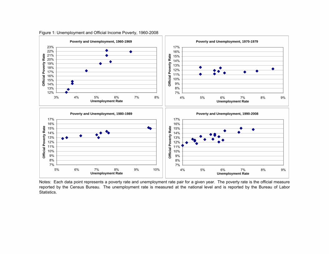
Figure 1: Unemployment and Official Income Poverty, 1960-2008

Notes: Each data point represents a poverty rate and unemployment rate pair for a given year. The poverty rate is the official measurereported by the Census Bureau. The unemployment rate is measured at the national level and is reported by the Bureau of LaborStatistics.

Poverty and Unemployment, 1960-1969

12%13%14%15%16%17%18%19%20%21%22%23%

3% 4% 5% 6% 7% 8%Unemployment Rate

Offi

cial

Pov

erty

Rat

ePoverty and Unemployment, 1970-1979

7%8%9%

10%11%12%13%14%15%16%17%


Offi

cial

Pov

erty

Rat

e


7%8%9%

10%11%12%13%14%15%16%17%


Offi

cial

Pov

erty

Rat

e


7%8%9%

10%11%12%13%14%15%16%17%


Offi

cial

Pov

erty

Rat

e

Figure 2: Unemployment and After-Tax Income or Consumption Poverty, 1963-2008

Notes: Each data point represents a poverty rate and unemployment rate pair for a given year. After-tax income poverty is calculatedusing data from the CPS, while consumption poverty is calculated using data from the CE Survey. Data for consumption poverty isreported for 1980, 1981, and 1984-2008.


15%16%17%18%19%20%21%22%23%24%25%


Pove

rty

Rat

e

After-Tax Income Poverty


7%8%9%

10%11%12%13%14%15%16%17%


Pove

rty

Rat

e



7%8%9%

10%11%12%13%14%15%16%17%


Pove

rty

Rat

e


Consumption Poverty


7%8%9%

10%11%12%13%14%15%16%17%


Pove

rty

Rat

e


Consumption Poverty

Table 1: Unemployment, Poverty, and the 10th Percentile, 1960-2008 National

Unemployment Rate

Official Income Poverty


Consumption Poverty

10th Percentile of After-Tax

Income

10th Percentile of Consumption

(1) (2) (3) (4) (5) (6)Year

1960 5.5 22.21961 6.7 21.9 20.6 10,7991963 5.7 19.5 25.0 8,0161972 5.6 11.9 14.2 14.2 11,832 12,8601975 8.5 12.3 13.9 12,2011980 7.1 13.0 13.0 13.0 12,466 13,2471985 7.2 14.0 14.5 14.0 11,548 12,6681990 5.6 13.5 12.6 13.1 12,402 13,2041995 5.6 13.8 11.3 12.5 13,349 13,5222000 4.0 11.3 8.8 10.3 15,462 14,3912005 5.1 12.6 9.7 9.1 14,731 15,0342008 5.8 13.2 10.2 7.7 14,306 15,592

1961-1972 -1.1 -10.0 -6.4 19.1%1963-1972 -0.1 -7.6 -10.7 47.6%1972-1980 1.5 1.1 -1.2 -1.2 5.4% 3.0%1980-1990 -1.5 0.5 -0.4 0.1 -0.5% -0.3%1990-2000 -1.6 -2.2 -3.9 -2.8 24.7% 9.0%2000-2008 1.8 1.9 1.4 -2.5 -7.5% 8.3%

Notes: The statistics in columns 3-6 are based on the authors' calculations using CPS data for income or CESurvey data for consumption. The poverty rates in columns 3 and 4 are anchored at the official rate in 1980, asexplained in the text. The 10th percentiles in columns 5 and 6 are expressed in constant 2005 dollars using the CPI-U-RS, adjusted for family size, and normalized to a three person family with one adult and two children.

Percent Change or Difference

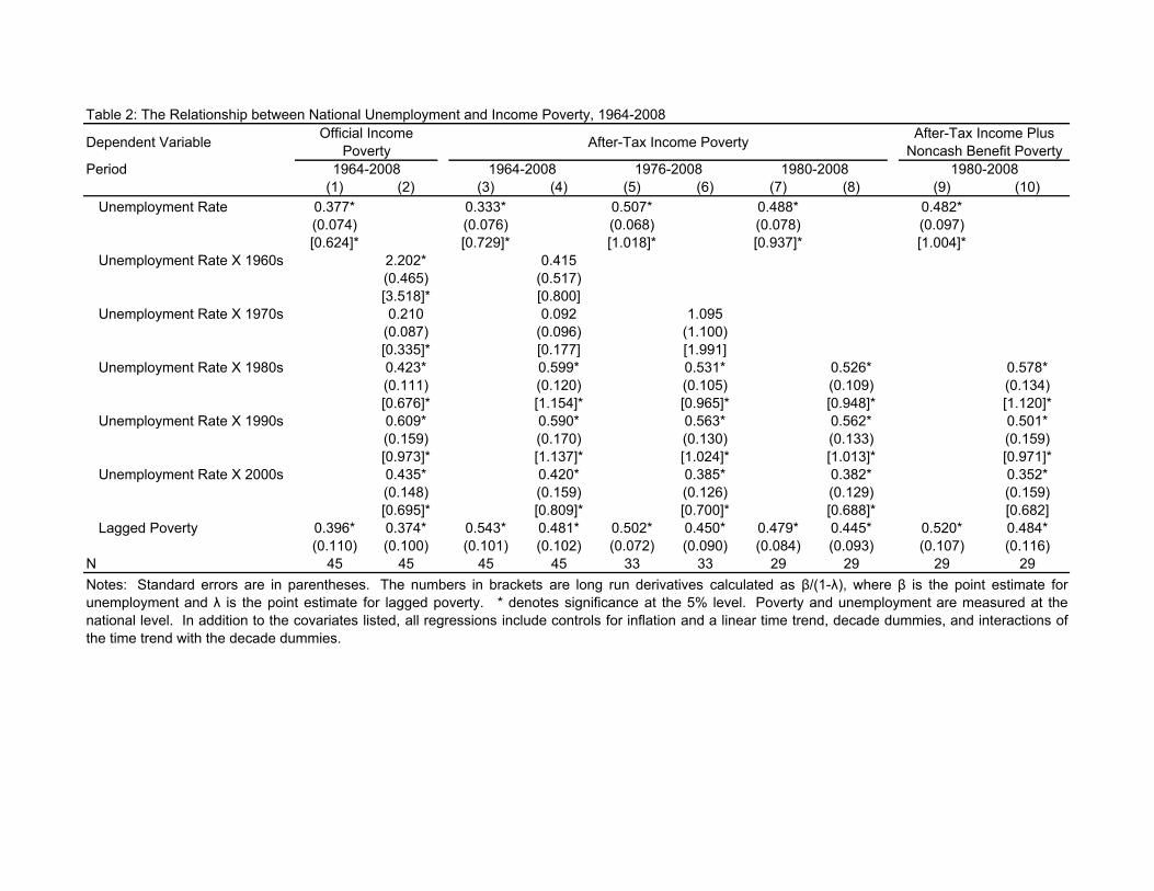
Table 2: The Relationship between National Unemployment and Income Poverty, 1964-2008

Dependent Variable Official Income Poverty After-Tax Income Poverty

After-Tax Income Plus Noncash Benefit Poverty

Period 1964-2008 1964-2008 1976-2008 1980-2008 1980-2008(1) (2) (3) (4) (5) (6) (7) (8) (9) (10)

Unemployment Rate 0.377* 0.333* 0.507* 0.488* 0.482*(0.074) (0.076) (0.068) (0.078) (0.097)[0.624]* [0.729]* [1.018]* [0.937]* [1.004]*

Unemployment Rate X 1960s 2.202* 0.415(0.465) (0.517)[3.518]* [0.800]

Unemployment Rate X 1970s 0.210 0.092 1.095(0.087) (0.096) (1.100)[0.335]* [0.177] [1.991]

Unemployment Rate X 1980s 0.423* 0.599* 0.531* 0.526* 0.578*(0.111) (0.120) (0.105) (0.109) (0.134)[0.676]* [1.154]* [0.965]* [0.948]* [1.120]*

Unemployment Rate X 1990s 0.609* 0.590* 0.563* 0.562* 0.501*(0.159) (0.170) (0.130) (0.133) (0.159)[0.973]* [1.137]* [1.024]* [1.013]* [0.971]*

Unemployment Rate X 2000s 0.435* 0.420* 0.385* 0.382* 0.352*(0.148) (0.159) (0.126) (0.129) (0.159)[0.695]* [0.809]* [0.700]* [0.688]* [0.682]

Lagged Poverty 0.396* 0.374* 0.543* 0.481* 0.502* 0.450* 0.479* 0.445* 0.520* 0.484*(0.110) (0.100) (0.101) (0.102) (0.072) (0.090) (0.084) (0.093) (0.107) (0.116)

N 45 45 45 45 33 33 29 29 29 29Notes: Standard errors are in parentheses. The numbers in brackets are long run derivatives calculated as β/(1-λ), where β is the point estimate forunemployment and λ is the point estimate for lagged poverty. * denotes significance at the 5% level. Poverty and unemployment are measured at thenational level. In addition to the covariates listed, all regressions include controls for inflation and a linear time trend, decade dummies, and interactions ofthe time trend with the decade dummies.

Table 3: The Relationship between Regional Unemployment and Income Poverty, 1976-2008

Dependent VariableOfficial Income

Poverty After-Tax Income Poverty After-Tax Income Plus

Noncash Benefit PovertyPeriod 1976-2008 1976-2008 1980-2008 1980-2008

(1) (2) (3) (4) (5) (6) (7) (8)Unemployment Rate 0.231* 0.178* 0.264* 0.272*

(0.070) (0.062) (0.077) (0.090)[1.095]* [1.113]* [1.222]* [1.277]*

Unemployment Rate X 1976-79 -0.028 -0.048(0.135) (0.127)[-0.104] [-0.241]

Unemployment Rate X 1980s 0.272* 0.243* 0.227* 0.248*(0.113) (0.104) (0.107) (0.126)[1.015]* [1.221]* [1.032]* [1.148]

Unemployment Rate X 1990s 0.465* 0.318* 0.329* 0.321*(0.145) (0.131) (0.138) (0.163)[1.735]* [1.598]* [1.495]* [1.486]*

Unemployment Rate X 2000s 0.434 0.259 0.205 0.183(0.250) (0.230) (0.237) (0.279)[1.619] [1.302] [0.932] [0.847]

Lagged Poverty 0.789* 0.732* 0.840* 0.801* 0.784* 0.780* 0.787* 0.784*(0.052) (0.055) (0.042) (0.046) (0.052) (0.054) (0.056) (0.058)

N 132 132 132 132 116 116 116 116Notes: Standard errors are in parentheses. The numbers in brackets are long run derivatives calculated as β/(1-λ), where β is thepoint estimate for unemployment and λ is the point estimate for lagged poverty. * denotes significance at the 5% level. Poverty andunemployment are measured at the regional level. In addition to the covariates listed, all regressions include region and year fixedeffects, and the specifications in even columns include decade dummies.

Table 4: The Relationship between Unemployment and Income and Consumption Poverty

National Level Poverty Regional Level Poverty

Dependent Variable After-Tax Income Poverty Consumption Poverty After-Tax Income

PovertyConsumption

Poverty1963-2008

1981-2008

1981-2008

1961-2008

1981-2008

1981-2008 1981-2008 1981-2008

(1) (2) (3) (4) (5) (6) (7) (8) (9) (10)Unemployment Rate 0.821* 0.512* 0.476*¹ 0.242 0.288* 0.540*

(0.256) (0.078) (0.142) (0.144) (0.078) (0.185)[0.874]* [0.281] [1.103]* [1.208]*

Unemployment Rate X 1980s 1.062* 1.002 0.290* -0.033(0.358) (0.672) (0.115) (0.273)[1.569]* [1.133] [1.090]* [-0.069]

Unemployment Rate X 1990s 0.734* 0.334 0.310* 1.079*¹(0.109) (0.234) (0.111) (0.278)[1.084]* [0.378]¹ [1.165]* [2.257]*

Unemployment Rate X 2000s 0.413* 0.284 0.195 0.974(0.090) (0.167) (0.189) (0.492)[0.610]* [0.321] [0.733] [2.038]*

Lagged Poverty 0.414* 0.323* 0.138 0.116 0.739* 0.734* 0.553* 0.522*(0.073) (0.074) (0.154) (0.176) (0.052) (0.052) (0.082) (0.080)

N 30 25 25 30 25 25 100 100 100 100Notes: Corresponding income and consumption equations were estimated simultaneously using SUR. Standard errors are in parentheses.The numbers in brackets are long run derivatives calculated as β/(1-λ), where β is the point estimate for unemployment and λ is the pointestimate for lagged poverty. * denotes significance at the 5% level. 1 denotes that the effect for consumption is significantly different fromthat for income. In columns 1-6, poverty and unemployment are determined at the national level, and specifications include inflation, a lineartime trend, decade dummies, and interactions of the time trend with the decade dummies. In columns 7-10, poverty and unemployment aredetermined at the regional level, and specifications include region and year fixed effects. Columns 8 and 10 also include decade dummies.For comparability across measures, we use data from years when both income and consumption data are available. For the full time periodthese years are 1961 or 1963, 1972, 1973, 1980, 1981, and 1984-2008.

Table 5A: The Relationship between Unemployment and the 10th Percentile of Log Income and Consumption

National Level Regional Level

Dependent Variable 10th Percentile of Log After-Tax Income

10th Percentile of Log Consumption

10th Percentile of Log After-Tax

Income


1963-2008

1981-2008

1981-2008

1961-2008

1981-2008

1981-2008 1981-2008 1981-2008

(1) (2) (3) (4) (5) (6) (7) (8) (9) (10)Unemployment Rate -0.040* -0.026* -0.015*¹ -0.008¹ -0.029* -0.020*

(0.009) (0.005) (0.004) (0.005) (0.005) (0.006)[-0.045]* [-0.009]*¹ [-0.063]* [-0.043]*

Unemployment Rate X 1980s -0.051* -0.036 -0.032* -0.002¹(0.024) (0.022) (0.007) (0.008)

[-0.079]* [-0.037] [-0.068]* [-0.004]¹Unemployment Rate X 1990s -0.036* -0.011¹ -0.028* -0.038*

(0.008) (0.007) (0.007) (0.008)[-0.056]* [-0.011]¹ [-0.059]* [-0.075]*

Unemployment Rate X 2000s -0.023* -0.011* -0.023* -0.038*(0.006) (0.005) (0.011) (0.015)

[-0.036]* [-0.011]¹ [-0.049]* [-0.075]*Lagged 10th Percentile 0.418* 0.353* 0.070 0.037 0.543* 0.527* 0.539* 0.492*

(0.079) (0.087) (0.167) (0.184) (0.057) (0.057) (0.078) (0.075)N 30 25 25 30 25 25 100 100 100 100

Notes: Corresponding income and consumption equations were estimated simultaneously using SUR. Standard errors are in parentheses.The numbers in brackets are long run derivatives calculated as β/(1-λ), where β is the point estimate for unemployment and λ is the pointestimate for the lagged 10th percentile. * denotes significance at the 5% level. 1 denotes that the effect for consumption is significantlydifferent from that for income. In columns 1-6, the 10th percentile and unemployment are determined at the national level, andspecifications include inflation, a linear time trend, decade dummies, and interactions of the time trend with the decade dummies. Incolumns 7-10, the 10th percentile and unemployment are determined at the regional level, and specifications include region and year fixedeffects. Columns 8 and 10 also include decade dummies. For comparability across measures, we use data from years when both incomeand consumption data are available. For the full time period these years are 1961 or 1963, 1972, 1973, 1980, 1981, and 1984-2008.

Table 5B: The Relationship between Unemployment and the 5th Percentile of Log Income and Consumption





Income


1963-2008

1981-2008

1981-2008

1961-2008

1981-2008

1981-2008 1981-2008 1981-2008

(1) (2) (3) (4) (5) (6) (7) (8) (9) (10)Unemployment Rate -0.058* -0.061* -0.013*¹ 0.000¹ -0.042* -0.023*

(0.015) (0.010) (0.005) (0.005) (0.009) (0.007)[-0.086]* [0.000]¹ [-0.102]* [-0.065]*

Unemployment Rate X 1980s -0.021 -0.066 -0.041* 0.004¹(0.048) (0.022) (0.014) (0.010)[-0.027] [-0.044]* [-0.097]* [0.009]¹

Unemployment Rate X 1990s -0.059* -0.007¹ -0.044* -0.048*(0.014) (0.006) (0.013) (0.010)

[-0.077]* [-0.005]¹ [-0.105]* [-0.110]*Unemployment Rate X 2000s -0.059* -0.003¹ -0.043 -0.062*

(0.012) (0.006) (0.023) (0.018)[-0.077]* [-0.002]¹ [-0.102] [-0.143]*

Lagged 5th Percentile 0.292* 0.234* -0.431* -0.514* 0.590* 0.579* 0.644* 0.565*(0.088) (0.088) (0.207) (0.173) (0.065) (0.066) (0.078) (0.075)

N 30 25 25 30 25 25 100 100 100 100Notes: See notes to Table 5A.

Table 5C: The Relationship between Unemployment and the 15th Percentile of Log Income and Consumption





Income


1963-2008

1981-2008

1981-2008

1961-2008

1981-2008

1981-2008 1981-2008 1981-2008

(1) (2) (3) (4) (5) (6) (7) (8) (9) (10)Unemployment Rate -0.036* -0.023* -0.014*¹ -0.006¹ -0.019* -0.015*

(0.008) (0.004) (0.004) (0.004) (0.003) (0.005)[-0.043]* [-0.007]¹ [-0.058]* [-0.033]*

Unemployment Rate X 1980s -0.052* -0.016 -0.021* 0.002¹(0.018) (0.020) (0.005) (0.008)

[-0.081]* [-0.019] [-0.062]* [0.004]¹Unemployment Rate X 1990s -0.034* -0.006¹ -0.017* -0.030*

(0.006) (0.007) (0.005) (0.008)[-0.053]* [-0.007]¹ [-0.050]* [-0.061]*

Unemployment Rate X 2000s -0.018* -0.008 -0.016* -0.027(0.004) (0.005) (0.008) (0.014)

[-0.028]* [-0.010] [-0.047]* [-0.055]Lagged 15th Percentile 0.460* 0.356* 0.154 0.177 0.671* 0.659* 0.550* 0.505*

(0.079) (0.081) (0.147) (0.171) (0.050) (0.050) (0.079) (0.078)N 30 25 25 30 25 25 100 100 100 100Notes: See notes to Table 5A.

Table 6: The Relationship between Unemployment and Income and Consumption Relative Poverty

National Level Poverty Regional Level Poverty

Dependent Variable After-Tax Income Relative Poverty

Consumption Relative Poverty

After-Tax Income Relative Poverty

Consumption Relative Poverty

1963-2008

1981-2008

1981-2008

1961-2008

1981-2008

1981-2008 1981-2008 1981-2008

(1) (2) (3) (4) (5) (6) (7) (8) (9) (10)Unemployment Rate 0.156 0.173 0.107 -0.214 0.240* 0.371*

(0.082) (0.095) (0.096) (0.161) (0.088) (0.174)[0.210] [-0.186]¹ [0.654]* [0.890]*

Unemployment Rate X 1980s 0.369 1.203 0.279* -0.168(0.472) (0.665) (0.137) (0.248)[0.418] [0.872] [0.723]* [-0.381]

Unemployment Rate X 1990s 0.293* -0.237¹ 0.258* 0.899*¹(0.136) (0.209) (0.124) (0.251)[0.332]* [-0.172]¹ [0.668]* [2.039]*

Unemployment Rate X 2000s 0.095 -0.060 0.048 0.682(0.121) (0.173) (0.216) (0.445)[0.108] [-0.043] [0.124] [1.546]

Lagged Poverty 0.178 0.118 -0.151 -0.380 0.633* 0.614* 0.583* 0.559*(0.155) (0.155) (0.382) (0.355) (0.070) (0.071) (0.086) (0.083)

N 30 25 25 30 25 25 100 100 100 100Notes: The consumption (income) relative poverty rate is defined as the fraction of individuals with consumption (income) below 50 percentof median consumption (income). See Table 4 for additional notes.

Appendix Table 1: The Relationship between GDP per Capita and Income and Consumption Poverty

National Level Poverty Regional Level Poverty (1981-2008)Dependent Variable After-Tax Income Poverty Consumption Poverty After-Tax Income Poverty Consumption Poverty

Level Level Level Level Level Level Level LevelFirst

Difference Level Level Level Level1963-2008 1981-2008

1981-2008

1961-2008

1981-2008

1981-2008 1981-2008 1981-2008

(1) (2) (3) (4) (5) (6) (7) (8) (9) (10) (11) (12) (13)Log GDP per Capita -54.436* -14.996* -27.903*¹ -5.002 -10.117* 0.899 3.022 -30.582* -18.127*

(5.453) (4.378) (3.361) (6.049) (3.209) (1.716) (1.640) (4.301) (4.929)[-25.417]* [-5.927]¹ [5.549] [-30.466]*

Log GDP per Capita X 1980s 7.124 39.199 -1.640 -21.712*(45.755) (59.557) (1.883) (5.039)[12.368] [43.554] [-6.721] [-33.925]*¹

Log GDP per Capita X 1990s -15.051* -10.587 3.439 -16.345*(6.948) (11.769) (1.771) (5.321)

[-26.130]* [-11.763] [14.094] [-25.539]*¹Log GDP per Capita X 2000s -15.245* -2.158 1.399 -15.014*

(6.264) (8.158) (1.732) (5.088)[-26.467]* [-2.398] [5.734] [-23.459]*¹

Lagged Poverty 0.410* 0.424* 0.156 0.100 0.838* 0.756* 0.405* 0.360*(0.101) (0.122) (0.159) (0.231) (0.049) (0.060) (0.095) (0.095)

N 30 25 25 30 25 25 100 100 100 100 100 100 100Notes: The dependent variable is either the poverty rate (level) or the change in the poverty rate from the previous year (first difference). See Table 4 for additional notes.

Documents

Consumption and Income Poverty over the Business … · Consumption and Income Poverty over the Business Cycle ... off-the-books income, inter-family ... exploit both regional and