SLCC MATH 1040 FINAL EXAM FALL 2015 NAME: _________________________

Form A INSTRUCTOR: ________________________

1

TEST INSTRUCTIONS:

This exam consists of both "multiple choice" and "free response" questions. For "free

response" questions, you must support your answer with relevant work. Work for these

problems must be shown on the exam. Work carefully and neatly, appropriately

justifying your solutions. Partial credit may be awarded for relevant work on "free

response" problems.

You may not use your own notes, books, headphones, phones, nor any device that

connects to the internet. Any calculator may be used and formulas are provided. You

have 120 minutes to complete this exam.

1) Suppose that a study finds that the average pop song length in America is 4 minutes

with a standard deviation of 1.25 minutes. It is known that song length is not normally

distributed. If 100 pop songs are selected at random, find the probability that their mean

length will be longer than 4.25 minutes.

a. 0.5793

b. 0.4207

c. 0.0228

d. 0.9772

2) A histogram of a set of data indicates that the distribution of the data is skewed right.

Which measure of central tendency will likely be larger, the mean or the median? Why?

a. The median will likely be larger because the extreme values in the left tail tend to

pull the median in the opposite direction of the tail.

b. The mean will likely be larger because the extreme values in the right tail tend to

pull the mean in the direction of the tail.

c. The median will likely be larger because the extreme values in the right tail tend

to pull the median in the direction of the tail.

d. The mean will likely be larger because the extreme values in the left tail tend to

pull the mean in the opposite direction of the tail.

2

3) The authors of the paper “Fudging the Numbers: Distributing Chocolate Influences

Student Evaluations of an Undergraduate Course” (Teaching in Psychology [2007]:

245-247) carried out a study to see if events unrelated to an undergraduate course could

affect student evaluation. Students enrolled in statistics courses taught by the same

instructor participated in the study. All students attended the same lectures and one of

six discussion sections that met once a week. At the end of the course, the researchers

randomly choose three of the discussion sections to be the “chocolate group.” Students

in these three sections were offered chocolate prior to having them fill out course

evaluations. Students in the other three sections were not offered chocolate. The

researchers concluded that “Overall, students offered chocolate gave more positive

evaluations than students not offered chocolate.” Is this study an observational study or

an experiment?

a. Observational Study because all the students attended the same lectures and

discussion sections.

b. Experiment, because sections were randomly chosen.

c. Observational Study, because students could choose to take the chocolate or not.

d. Experiment, because a treatment was applied to three sections.

4) The average number of hours spent completing statistics homework for a randomly

selected group of SLCC statistics students is an example of what type of data?

a. Quantitative Data

b. Binomial Data

c. Qualitative/Categorical Data

d. Interval Data

e. None of these

5) Suppose we construct a confidence interval for p , the proportion of Salt Lake

Community College students who live more than 25 miles from Redwood campus.

What would the effect be on the margin of error of the confidence interval if we

reduced our sample size from 400 to 200?

a. The margin of error would be smaller.

b. The margin of error would remain the same.

c. The margin of error would increase.

d. It is impossible to tell from the information provided.

3

6) Suppose that a recent poll of American households about pet ownership found that for

households with one pet, 39% owned a dog, 33% owned a cat, 7% owned a bird, and the

remaining households in the sample owned some other pet. Suppose that three

households are selected randomly and with replacement. What is the probability that

none of the three randomly selected households own a bird?

a. 0.210

b. 0.930

c. 0.804

d. 0.790

e. None of these

7) A random sample of 1345 adult television viewers showed that 52% planned to watch

the NCAA finals. The margin of error is 3 percentage points with a 95% confidence.

Does the confidence interval support the claim that the majority of adult television

viewers plan to watch the NCAA finals? Why?

a. Yes; the confidence interval means that we are 95% confident that the population

proportion of adult television viewers who plan to watch the NCAA finals is

between 50.5% and 53.5%. Since the entire interval is above 50%, this is sufficient

evidence that the true proportion is greater than 50%.

b. Yes; the confidence interval means that we are 95% confident that the population

proportion of adult television viewers who plan to watch the NCAA finals is

between 49% and 55%. Since the confidence interval is mostly above 50% it is

likely that the true proportion is greater than 50%.

c. No; the confidence interval means that we are 95% confident that the population

proportion of adult television viewers who plan to watch the NCAA finals is

between 50.5% and 53.5%. The lower limit of the confidence interval is just too

close to 50% to say for sure.

d. No; the confidence interval means that we are 95% confident that the population

proportion of adult television viewers who plan to watch the NCAA finals is

between 49% and 55%. The true proportion could be less than 50%.

4

8) The following relative frequency histogram and table display the square footage for 40

homes sold in Dutchess County, New York.

Area Relative

Frequency

1000-1499 0.200

1500-1999 0.325

2000-2499 0.250

2500-2999 0.125

3000-3499 0.075

3500-3999 0.025

i. What is the class width?

ii. What percentage of homes sold had less than 2500 square feet?

9) A bag contains 10 white, 12 blue, 13 red, 7 yellow, and 8 green wooden balls.

i. Method 1: A ball is selected from the bag, its color noted, then replaced in the

bag. You then draw a second ball, note its color and then replace the ball. What is

the probability of selecting 2 red balls? Round to the nearest ten-thousandth.

ii. Method 2: A ball is selected from the bag, its color noted, then without replacing

the ball, a second ball is drawn from the bag and its color noted. What is the

probability of selecting 2 red balls? Round to the nearest ten-thousandth.

5

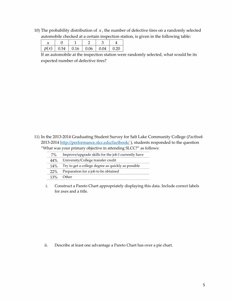
10) The probability distribution of x , the number of defective tires on a randomly selected

automobile checked at a certain inspection station, is given in the following table:

x 0 1 2 3 4

( )p x 0.54 0.16 0.06 0.04 0.20

If an automobile at the inspection station were randomly selected, what would be its

expected number of defective tires?

11) In the 2013-2014 Graduating Student Survey for Salt Lake Community College (Factbook

2013-2014 http://performance.slcc.edu/factbook/ ), students responded to the question

“What was your primary objective in attending SLCC?” as follows:

i. Construct a Pareto Chart appropriately displaying this data. Include correct labels

for axes and a title.

ii. Describe at least one advantage a Pareto Chart has over a pie chart.

7% Improve/upgrade skills for the job I currently have

44% University/College transfer credit

14% Try to get a college degree as quickly as possible

22% Preparation for a job to be obtained

13% Other

6

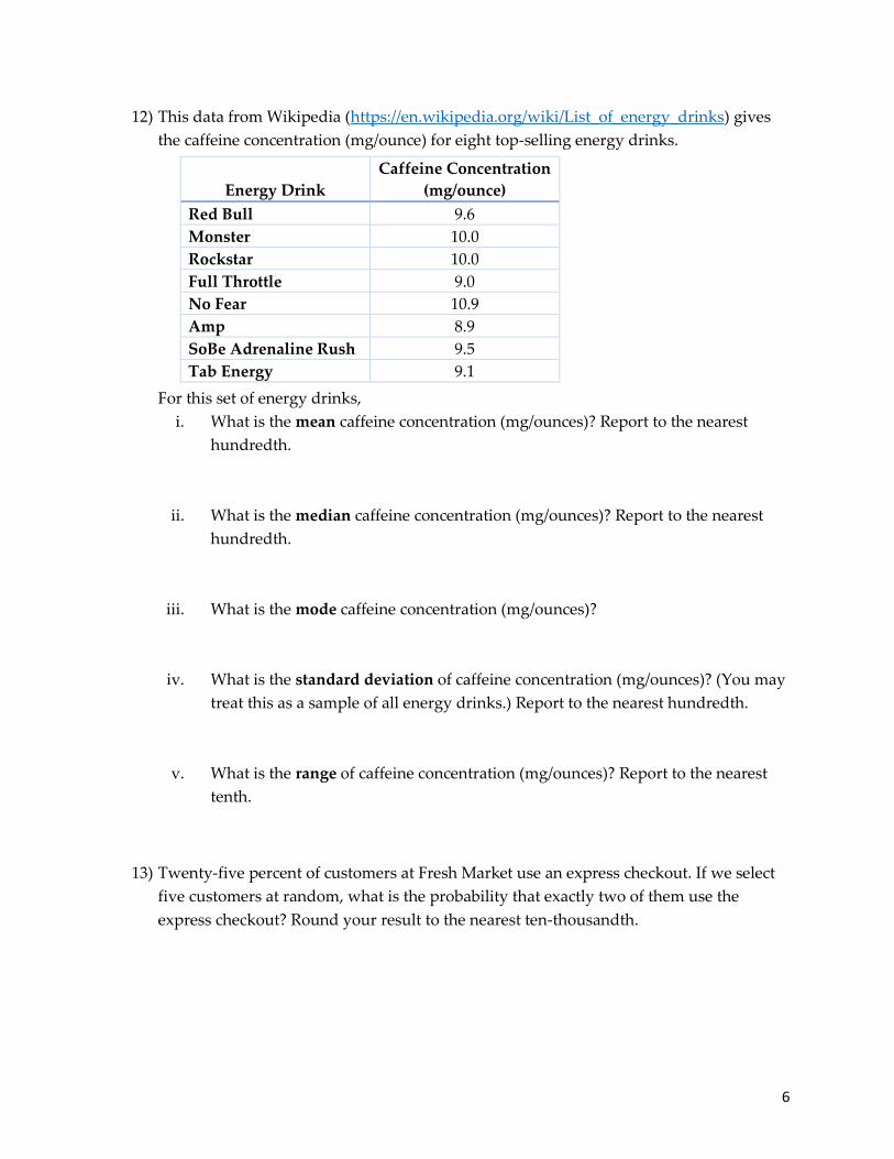
12) This data from Wikipedia (https://en.wikipedia.org/wiki/List_of_energy_drinks) gives

the caffeine concentration (mg/ounce) for eight top-selling energy drinks.

For this set of energy drinks,

i. What is the mean caffeine concentration (mg/ounces)? Report to the nearest

hundredth.

ii. What is the median caffeine concentration (mg/ounces)? Report to the nearest

hundredth.

iii. What is the mode caffeine concentration (mg/ounces)?

iv. What is the standard deviation of caffeine concentration (mg/ounces)? (You may

treat this as a sample of all energy drinks.) Report to the nearest hundredth.

v. What is the range of caffeine concentration (mg/ounces)? Report to the nearest

tenth.

13) Twenty-five percent of customers at Fresh Market use an express checkout. If we select

five customers at random, what is the probability that exactly two of them use the

express checkout? Round your result to the nearest ten-thousandth.

Energy Drink

Caffeine Concentration

(mg/ounce)

Red Bull 9.6

Monster 10.0

Rockstar 10.0

Full Throttle 9.0

No Fear 10.9

Amp 8.9

SoBe Adrenaline Rush 9.5

Tab Energy 9.1

7

14) The article “That’s Rich: More You Drink, More You Earn” (Calgary Herald, April 2002)

reported that there was a positive correlation between alcohol consumption and income.

Is it reasonable to conclude that increasing alcohol consumption will cause an increase in

income? Explain why or why not using a statistical argument.

15) A study reported by the Associated Press on April 3, 2002 reported that out of a

representative sample of 2,013 American adults, 1,556 of them indicated that a lack of

respect and courtesy in American society is a serious problem. Is there convincing

evidence that more than 75% of American adults believe that a lack of respect and

courtesy is a serious problem? Test the appropriate hypotheses using the p-value

method, with a significance level of 0.05.

i. Null Hypothesis:

ii. Alternative Hypothesis:

iii. Test Statistic:

iv. p-value (report to the nearest ten-thousandth):

v. Conclusion about the Null Hypothesis:

vi. Conclusion addressing the original claim (complete sentence):

8

16) The time that it takes a randomly selected job applicant to assemble a calculator has a

distribution that can be approximated by a normal distribution with a mean of 120

seconds and a standard deviation of 20 seconds. The 10% of applicants with the shortest

times are to be given advanced training in calculator assembly. What task time qualifies

individuals for such training?

Report the time to the nearest tenth of a second. Include an appropriately labeled sketch

of the normal curve in your solution for this problem.

17) A manufacturer of college textbooks is interested in testing the strength of the bindings

produced by a particular binding machine. Strength of the binding can be measured by

recording the force required to pull the pages from the binding. If this force is measured

in pounds, how many books should be tested to estimate the average force required to

break the binding with a margin of error of 0.1 pound at a 95% confidence level?

Assume that is known to be 0.7 pounds.

18) A city manager claims that the mean age of bus drivers in Salt Lake City is over 52 years.

Both in statistics notation and in words, write the appropriate null and alternative

hypotheses for testing this claim.

9

19) A student randomly selects 10 paperbacks at a Barnes and Noble bookstore. She finds

the mean price to be $8.75 with a standard deviation of $1.50. Construct a 95%

confidence interval for the population standard deviation, . Report the confidence

interval limits to the nearest cent. Assume that the price of paperback books at the

bookstore follows a normal distribution.

20) The article “Air Pollution and Medical Care Use by Older Americans” (Health Affairs

[2002]: 207-214) gave data on a measure of pollution (in micrograms of particulate

matter per cubic meter of air) and the cost of medical care per person over age 65 for six

geographical regions of the United States:

Region Pollution Cost of Medical Care

North 30.0 $964

Upper South 31.8 $926

Deep South 32.1 $968

West South 26.8 $972

Big Sky 30.4 $952

West 40.0 $899

i. Find the equation of the least squares regression line for predicting the medical

cost using pollution. Report the coefficients to the nearest hundredth.

ii. Use a complete sentence to interpret the slope of your regression line in the

context of the data.

iii. Would you use the least squares regression equation to predict cost of medical

care for a region that has a pollution measure of 60.0? If so, what is the predicted

cost of medical care? If not, explain why.

Statistics Formulas and Tables Descriptive Statistics Probability

�̅� =∑ 𝑥

𝑛 mean

�̅� =∑(𝑓∙𝑥)

∑ 𝑓 approximate mean from a frequency table

𝑠 = √∑(𝑥−�̅�)2

𝑛−1 standard deviation

𝑠 = √∑(𝑥𝑖−�̅�)2∙𝑓𝑖

∑ 𝑓𝑖−1 approx. std. dev. from a frequency table

variance = 𝑠2

Interquartile Range: 𝐼𝑄𝑅 = 𝑄3 − 𝑄1

Lower fence = 𝑄1 − 1.5(𝐼𝑄𝑅)

Upper fence = 𝑄3 + 1.5(𝐼𝑄𝑅)

General Addition Rule 𝑃(𝐴 𝑜𝑟 𝐵) = 𝑃(𝐴) + 𝑃(𝐵) − 𝑃(𝐴 𝑎𝑛𝑑 𝐵)

multiplication rule for independent events 𝑃(𝐴 𝑎𝑛𝑑 𝐵) = 𝑃(𝐴) ∙ 𝑃(𝐵)

multiplication rule for dependent events 𝑃(𝐴 𝑎𝑛𝑑 𝐵) = 𝑃(𝐴) ∙ 𝑃(𝐵|𝐴)

complement rule 𝑃(�̅�) = 1 − 𝑃(𝐴)

𝑃𝑟𝑛 =𝑛!

(𝑛−𝑟)! Permutations (no elements alike)

𝑛!

𝑛1!𝑛2!⋯𝑛𝑘! Permutations (𝑛1 alike, ⋯)

𝐶𝑟𝑛 =𝑛!

(𝑛−𝑟)!𝑟! Combinations

Probability Distributions Normal Distribution and Sampling Distributions

mean (expected value) of a discrete random variable 𝜇 = ∑[𝑥 ∙ 𝑃(𝑥)]

standard deviation of a discrete random variable

𝜎 = √∑[𝑥2 ∙ 𝑃(𝑥)] − 𝜇2

𝑃(𝑥) = 𝐶𝑥𝑛 ∙ 𝑝𝑥 ∙ (1 − 𝑝)𝑛−𝑥 Binomial probability

𝜇 = 𝑛 ∙ 𝑝 mean for a Binomial distribution

𝜎 = √𝑛 ∙ 𝑝 ∙ (1 − 𝑝) std. dev. for a Binomial distribution

𝑧 =𝑥−𝜇

𝜎 standard normal score

mean of the sampling distribution of �̅� 𝜇�̅� = 𝜇 std. dev. of the sampling distribution of �̅� (std. error)

𝜎�̅� =𝜎

√𝑛

𝜇𝑝 = 𝑝 mean of the sampling distribution of �̂�

𝜎𝑝 = √𝑝(1−𝑝)

𝑛 std. dev. of the sampling distribution of �̂�

Estimating a Population Parameter Hypothesis Testing

Proportion:

ˆ ˆp E p p E where

2

ˆ ˆ1p pE z

n

2

2

2

0.25zn

E

sample size, �̂� unknown

2

2

2

ˆ ˆ1z p pn

E

sample size, �̂� known

Mean:

x E x E where 2

sE t

n

2

2zn

E

sample size

Standard Deviation:

2 2

2 2

1 1

R L

n s n s

ˆ

1

p pz

p p

n

proportion – one population

xt

s

n

mean – one population

Linear Correlation and Regression

𝑟 = linear correlation coefficient

𝑟 =∑(

𝑥𝑖−�̅�

𝑠𝑥)(

𝑦𝑖−�̅�

𝑠𝑦)

𝑛−1

�̂� = 𝑏0 + 𝑏1𝑥 estimated eqn. of linear regression line

𝑅2 = 𝑟2 coefficient of determination

Residual = 𝑦 − �̂�

Ch. 13: Nonparametric Tests

z =

(x + 0.5) - (n>2)

1n

2

Sign test for n 7 25

z =

T - n (n + 1)>4

Bn (n + 1)(2n + 1)

24

Formulas and Tables by Mario F. Triola

Copyright 2014 Pearson Education, Inc.

z =

R - mR

sR

=

R-

n1(n1 + n2 + 1)

2

Bn1n2(n1 + n2 + 1)

12

Wilcoxon rank-sum

(two independent

samples)

H =

12

N(N + 1) aR2

1

n1

+

R22

n2

+ . . . +

R2k

nk

b - 3(N + 1)

Kruskal-Wallis (chi-square df = k - 1)

rs = 1 -6Σd 2

n(n2- 1)

Rank correlation

acritical values for n 7 30: { z

1n - 1b

z =

G - mG

sG

=

G - a 2n1n2

n1 + n2

+ 1b

B(2n1n2)(2n1n2 - n1 - n2)

(n1 + n2)2(n1 + n2 - 1)

Runs test

for n 7 20

Ch. 14: Control Charts

R chart: Plot sample ranges

UCL: D4R

Centerline: R

LCL: D3R

x chart: Plot sample means

UCL: x + A2R

Centerline: x

LCL: x - A2R

p chart: Plot sample proportions

UCL: p + 3 Bp q

n

Centerline: p

LCL: p - 3 Bp q

n

Table A-6 Critical Values of the Pearson

Correlation Coefficient r

n a = 3 4 5 a = 3 4 64 .950 .990

5 .878 .959

6 .811 .917

7 .754 .875

8 .707 .834

9 .666 .798

10 .632 .765

11 .602 .735

12 .576 .708

13 .553 .684

14 .532 .661

15 .514 .641

16 .497 .623

17 .482 .606

18 .468 .590

19 .456 .575

20 .444 .561

25 .396 .505

30 .361 .463

35 .335 .430

40 .312 .402

45 .294 .378

50 .279 .361

60 .254 .330

70 .236 .305

80 .220 .286

90 .207 .269

100 .196 .256

NOTE: To test H0: r = 0 against H1: r ≠ 0, reject H0 if the absolute

value of r is greater than the critical value in the table.

Control Chart Constants

Subgroup Size      

n D3 D4 A2

2 0.000 3.267 1.880

3 0.000 2.574 1.023

4 0.000 2.282 0.729

5 0.000 2.114 0.577

6 0.000 2.004 0.483

7 0.076 1.924 0.419

Wilcoxon signed ranks

(matched pairs and n 7 30)

� � � � � � ! ! " # $ % # & � ' ' � ( ) � � * + , & & 0 ( � - . - ( . ( / � � 1 2

B-7

Table A-2 Standard Normal (z) Distribution: Cumulative Area from the LEFT

z .00 .01 .02 .03 .04 .05 .06 .07 .08 .09

-3.50 and

lower

.0001

                 

-3.4 .0003 .0003 .0003 .0003 .0003 .0003 .0003 .0003 .0003 .0002

-3.3 .0005 .0005 .0005 .0004 .0004 .0004 .0004 .0004 .0004 .0003

-3.2 .0007 .0007 .0006 .0006 .0006 .0006 .0006 .0005 .0005 .0005

-3.1 .0010 .0009 .0009 .0009 .0008 .0008 .0008 .0008 .0007 .0007

-3.0 .0013 .0013 .0013 .0012 .0012 .0011 .0011 .0011 .0010 .0010

-2.9 .0019 .0018 .0018 .0017 .0016 .0016 .0015 .0015 .0014 .0014

-2.8 .0026 .0025 .0024 .0023 .0023 .0022 .0021 .0021 .0020 .0019

-2.7 .0035 .0034 .0033 .0032 .0031 .0030 .0029 .0028 .0027 .0026

-2.6 .0047 .0045 .0044 .0043 .0041 .0040 .0039 .0038 .0037 .0036

-2.5 .0062 .0060 .0059 .0057 .0055 .0054 .0052 .0051 * .0049 .0048

-2.4 .0082 .0080 .0078 .0075 .0073 .0071 .0069 .0068 .0066 .0064

-2.3 .0107 .0104 .0102 .0099 .0096 .0094 .0091 .0089 .0087 .0084

-2.2 .0139 .0136 .0132 .0129 .0125 .0122 .0119 .0116 .0113 .0110

-2.1 .0179 .0174 .0170 .0166 .0162 .0158 .0154 .0150 .0146 .0143

-2.0 .0228 .0222 .0217 .0212 .0207 .0202 .0197 .0192 .0188 .0183

-1.9 .0287 .0281 .0274 .0268 .0262 .0256 .0250 .0244 .0239 .0233

-1.8 .0359 .0351 .0344 .0336 .0329 .0322 .0314 .0307 .0301 .0294

-1.7 .0446 .0436 .0427 .0418 .0409 .0401 .0392 .0384 .0375 .0367

-1.6 .0548 .0537 .0526 .0516 .0505 * .0495 .0485 .0475 .0465 .0455

-1.5 .0668 .0655 .0643 .0630 .0618 .0606 .0594 .0582 .0571 .0559

-1.4 .0808 .0793 .0778 .0764 .0749 .0735 .0721 .0708 .0694 .0681

-1.3 .0968 .0951 .0934 .0918 .0901 .0885 .0869 .0853 .0838 .0823

-1.2 .1151 .1131 .1112 .1093 .1075 .1056 .1038 .1020 .1003 .0985

-1.1 .1357 .1335 .1314 .1292 .1271 .1251 .1230 .1210 .1190 .1170

-1.0 .1587 .1562 .1539 .1515 .1492 .1469 .1446 .1423 .1401 .1379

-0.9 .1841 .1814 .1788 .1762 .1736 .1711 .1685 .1660 .1635 .1611

-0.8 .2119 .2090 .2061 .2033 .2005 .1977 .1949 .1922 .1894 .1867

-0.7 .2420 .2389 .2358 .2327 .2296 .2266 .2236 .2206 .2177 .2148

-0.6 .2743 .2709 .2676 .2643 .2611 .2578 .2546 .2514 .2483 .2451

-0.5 .3085 .3050 .3015 .2981 .2946 .2912 .2877 .2843 .2810 .2776

-0.4 .3446 .3409 .3372 .3336 .3300 .3264 .3228 .3192 .3156 .3121

-0.3 .3821 .3783 .3745 .3707 .3669 .3632 .3594 .3557 .3520 .3483

-0.2 .4207 .4168 .4129 .4090 .4052 .4013 .3974 .3936 .3897 .3859

-0.1 .4602 .4562 .4522 .4483 .4443 .4404 .4364 .4325 .4286 .4247

-0.0 .5000 .4960 .4920 .4880 .4840 .4801 .4761 .4721 .4681 .4641

NOTE: For values of z below -3.49, use 0.0001 for the area.

*Use these common values that result from interpolation:

z score Area

-1.645 0.0500

-2.575 0.0050

NEGATIVE z Scores0z

8056_Barrelfold_pp01-08.indd 1 9/26/12 9:52 AM

B-1

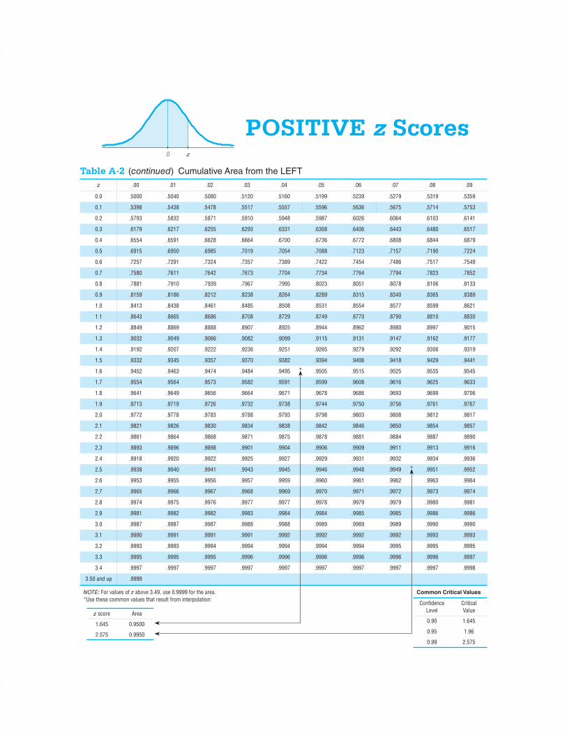
Table A-2 (continued) Cumulative Area from the LEFT

z .00 .01 .02 .03 .04 .05 .06 .07 .08 .09

0.0 .5000 .5040 .5080 .5120 .5160 .5199 .5239 .5279 .5319 .5359

0.1 .5398 .5438 .5478 .5517 .5557 .5596 .5636 .5675 .5714 .5753

0.2 .5793 .5832 .5871 .5910 .5948 .5987 .6026 .6064 .6103 .6141

0.3 .6179 .6217 .6255 .6293 .6331 .6368 .6406 .6443 .6480 .6517

0.4 .6554 .6591 .6628 .6664 .6700 .6736 .6772 .6808 .6844 .6879

0.5 .6915 .6950 .6985 .7019 .7054 .7088 .7123 .7157 .7190 .7224

0.6 .7257 .7291 .7324 .7357 .7389 .7422 .7454 .7486 .7517 .7549

0.7 .7580 .7611 .7642 .7673 .7704 .7734 .7764 .7794 .7823 .7852

0.8 .7881 .7910 .7939 .7967 .7995 .8023 .8051 .8078 .8106 .8133

0.9 .8159 .8186 .8212 .8238 .8264 .8289 .8315 .8340 .8365 .8389

1.0 .8413 .8438 .8461 .8485 .8508 .8531 .8554 .8577 .8599 .8621

1.1 .8643 .8665 .8686 .8708 .8729 .8749 .8770 .8790 .8810 .8830

1.2 .8849 .8869 .8888 .8907 .8925 .8944 .8962 .8980 .8997 .9015

1.3 .9032 .9049 .9066 .9082 .9099 .9115 .9131 .9147 .9162 .9177

1.4 .9192 .9207 .9222 .9236 .9251 .9265 .9279 .9292 .9306 .9319

1.5 .9332 .9345 .9357 .9370 .9382 .9394 .9406 .9418 .9429 .9441

1.6 .9452 .9463 .9474 .9484 .9495 * .9505 .9515 .9525 .9535 .9545

1.7 .9554 .9564 .9573 .9582 .9591 .9599 .9608 .9616 .9625 .9633

1.8 .9641 .9649 .9656 .9664 .9671 .9678 .9686 .9693 .9699 .9706

1.9 .9713 .9719 .9726 .9732 .9738 .9744 .9750 .9756 .9761 .9767

2.0 .9772 .9778 .9783 .9788 .9793 .9798 .9803 .9808 .9812 .9817

2.1 .9821 .9826 .9830 .9834 .9838 .9842 .9846 .9850 .9854 .9857

2.2 .9861 .9864 .9868 .9871 .9875 .9878 .9881 .9884 .9887 .9890

2.3 .9893 .9896 .9898 .9901 .9904 .9906 .9909 .9911 .9913 .9916

2.4 .9918 .9920 .9922 .9925 .9927 .9929 .9931 .9932 .9934 .9936

2.5 .9938 .9940 .9941 .9943 .9945 .9946 .9948 .9949 * .9951 .9952

2.6 .9953 .9955 .9956 .9957 .9959 .9960 .9961 .9962 .9963 .9964

2.7 .9965 .9966 .9967 .9968 .9969 .9970 .9971 .9972 .9973 .9974

2.8 .9974 .9975 .9976 .9977 .9977 .9978 .9979 .9979 .9980 .9981

2.9 .9981 .9982 .9982 .9983 .9984 .9984 .9985 .9985 .9986 .9986

3.0 .9987 .9987 .9987 .9988 .9988 .9989 .9989 .9989 .9990 .9990

3.1 .9990 .9991 .9991 .9991 .9992 .9992 .9992 .9992 .9993 .9993

3.2 .9993 .9993 .9994 .9994 .9994 .9994 .9994 .9995 .9995 .9995

3.3 .9995 .9995 .9995 .9996 .9996 .9996 .9996 .9996 .9996 .9997

3.4 .9997 .9997 .9997 .9997 .9997 .9997 .9997 .9997 .9997 .9998

3.50 and up .9999                  

NOTE: For values of z above 3.49, use 0.9999 for the area.

*Use these common values that result from interpolation:

Common Critical Values

Confidence Critical

z score Area              Level Value

1.645 0.9500              0.90 1.645

2.575 0.9950              0.95 1.96

                 0.99 2.575

POSITIVE z Scores0 z

8056_Barrelfold_pp01-08.indd 2 9/26/12 9:52 AM

B-2

Table A-3 t Distribution: Critical t Values

Area in One Tail

  0.005 0.01 0.025 0.05 0.10

Degrees of

Freedom

Area in Two Tails

0.01 0.02 0.05 0.10 0.20

1 63.657 31.821 12.706 6.314 3.078

2 9.925 6.965 4.303 2.920 1.886

3 5.841 4.541 3.182 2.353 1.638

4 4.604 3.747 2.776 2.132 1.533

5 4.032 3.365 2.571 2.015 1.476

6 3.707 3.143 2.447 1.943 1.440

7 3.499 2.998 2.365 1.895 1.415

8 3.355 2.896 2.306 1.860 1.397

9 3.250 2.821 2.262 1.833 1.383

10 3.169 2.764 2.228 1.812 1.372

11 3.106 2.718 2.201 1.796 1.363

12 3.055 2.681 2.179 1.782 1.356

13 3.012 2.650 2.160 1.771 1.350

14 2.977 2.624 2.145 1.761 1.345

15 2.947 2.602 2.131 1.753 1.341

16 2.921 2.583 2.120 1.746 1.337

17 2.898 2.567 2.110 1.740 1.333

18 2.878 2.552 2.101 1.734 1.330

19 2.861 2.539 2.093 1.729 1.328

20 2.845 2.528 2.086 1.725 1.325

21 2.831 2.518 2.080 1.721 1.323

22 2.819 2.508 2.074 1.717 1.321

23 2.807 2.500 2.069 1.714 1.319

24 2.797 2.492 2.064 1.711 1.318

25 2.787 2.485 2.060 1.708 1.316

26 2.779 2.479 2.056 1.706 1.315

27 2.771 2.473 2.052 1.703 1.314

28 2.763 2.467 2.048 1.701 1.313

29 2.756 2.462 2.045 1.699 1.311

30 2.750 2.457 2.042 1.697 1.310

31 2.744 2.453 2.040 1.696 1.309

32 2.738 2.449 2.037 1.694 1.309

33 2.733 2.445 2.035 1.692 1.308

34 2.728 2.441 2.032 1.691 1.307

35 2.724 2.438 2.030 1.690 1.306

36 2.719 2.434 2.028 1.688 1.306

37 2.715 2.431 2.026 1.687 1.305

38 2.712 2.429 2.024 1.686 1.304

39 2.708 2.426 2.023 1.685 1.304

40 2.704 2.423 2.021 1.684 1.303

45 2.690 2.412 2.014 1.679 1.301

50 2.678 2.403 2.009 1.676 1.299

60 2.660 2.390 2.000 1.671 1.296

70 2.648 2.381 1.994 1.667 1.294

80 2.639 2.374 1.990 1.664 1.292

90 2.632 2.368 1.987 1.662 1.291

100 2.626 2.364 1.984 1.660 1.290

200 2.601 2.345 1.972 1.653 1.286

300 2.592 2.339 1.968 1.650 1.284

400 2.588 2.336 1.966 1.649 1.284

500 2.586 2.334 1.965 1.648 1.283

1000 2.581 2.330 1.962 1.646 1.282

2000 2.578 2.328 1.961 1.646 1.282

Large 2.576 2.326 1.960 1.645 1.282

8056_Barrelfold_pp01-08.indd 3 9/26/12 9:52 AM

B-3

Table A-4 Chi-Square (x2) Distribution

Area to the Right of the Critical Value

Degrees of

Freedom

                   

0.995 0.99 0.975 0.95 0.90 0.10 0.05 0.025 0.01 0.005

1 — — 0.001 0.004 0.016 2.706 3.841 5.024 6.635 7.879

2 0.010 0.020 0.051 0.103 0.211 4.605 5.991 7.378 9.210 10.597

3 0.072 0.115 0.216 0.352 0.584 6.251 7.815 9.348 11.345 12.838

4 0.207 0.297 0.484 0.711 1.064 7.779 9.488 11.143 13.277 14.860

5 0.412 0.554 0.831 1.145 1.610 9.236 11.071 12.833 15.086 16.750

6 0.676 0.872 1.237 1.635 2.204 10.645 12.592 14.449 16.812 18.548

7 0.989 1.239 1.690 2.167 2.833 12.017 14.067 16.013 18.475 20.278

8 1.344 1.646 2.180 2.733 3.490 13.362 15.507 17.535 20.090 21.955

9 1.735 2.088 2.700 3.325 4.168 14.684 16.919 19.023 21.666 23.589

10 2.156 2.558 3.247 3.940 4.865 15.987 18.307 20.483 23.209 25.188

11 2.603 3.053 3.816 4.575 5.578 17.275 19.675 21.920 24.725 26.757

12 3.074 3.571 4.404 5.226 6.304 18.549 21.026 23.337 26.217 28.299

13 3.565 4.107 5.009 5.892 7.042 19.812 22.362 24.736 27.688 29.819

14 4.075 4.660 5.629 6.571 7.790 21.064 23.685 26.119 29.141 31.319

15 4.601 5.229 6.262 7.261 8.547 22.307 24.996 27.488 30.578 32.801

16 5.142 5.812 6.908 7.962 9.312 23.542 26.296 28.845 32.000 34.267

17 5.697 6.408 7.564 8.672 10.085 24.769 27.587 30.191 33.409 35.718

18 6.265 7.015 8.231 9.390 10.865 25.989 28.869 31.526 34.805 37.156

19 6.844 7.633 8.907 10.117 11.651 27.204 30.144 32.852 36.191 38.582

20 7.434 8.260 9.591 10.851 12.443 28.412 31.410 34.170 37.566 39.997

21 8.034 8.897 10.283 11.591 13.240 29.615 32.671 35.479 38.932 41.401

22 8.643 9.542 10.982 12.338 14.042 30.813 33.924 36.781 40.289 42.796

23 9.260 10.196 11.689 13.091 14.848 32.007 35.172 38.076 41.638 44.181

24 9.886 10.856 12.401 13.848 15.659 33.196 36.415 39.364 42.980 45.559

25 10.520 11.524 13.120 14.611 16.473 34.382 37.652 40.646 44.314 46.928

26 11.160 12.198 13.844 15.379 17.292 35.563 38.885 41.923 45.642 48.290

27 11.808 12.879 14.573 16.151 18.114 36.741 40.113 43.194 46.963 49.645

28 12.461 13.565 15.308 16.928 18.939 37.916 41.337 44.461 48.278 50.993

29 13.121 14.257 16.047 17.708 19.768 39.087 42.557 45.722 49.588 52.336

30 13.787 14.954 16.791 18.493 20.599 40.256 43.773 46.979 50.892 53.672

40 20.707 22.164 24.433 26.509 29.051 51.805 55.758 59.342 63.691 66.766

50 27.991 29.707 32.357 34.764 37.689 63.167 67.505 71.420 76.154 79.490

60 35.534 37.485 40.482 43.188 46.459 74.397 79.082 83.298 88.379 91.952

70 43.275 45.442 48.758 51.739 55.329 85.527 90.531 95.023 100.425 104.215

80 51.172 53.540 57.153 60.391 64.278 96.578 101.879 106.629 112.329 116.321

90 59.196 61.754 65.647 69.126 73.291 107.565 113.145 118.136 124.116 128.299

100 67.328 70.065 74.222 77.929 82.358 118.498 124.342 129.561 135.807 140.169

Source: From Donald B. Owen, Handbook of Statistical Tables.

Formulas and Tables by Mario F. Triola

Copyright 2014 Pearson Education, Inc.

Degrees of Freedom

n - 1 Confidence Interval or Hypothesis Test with a standard deviation or variance

k - 1 Goodness-of-Fit with k categories

(r - 1)(c - 1) Contingency Table with r rows and c columns

k - 1 Kruskal-Wallis test with k samples

8056_Barrelfold_pp01-08.indd 4 9/26/12 9:52 AM

B-4