Single Frequency Network Structural Aspects & … Frequency Network, #6 next level solutions 3-Dec-15 TX Network Adapter RX Network Adapter Distribution Network SYNC system Maximum

Single Frequency Network Structural Aspects & Practical Field

ConsiderationsNovember 2011

Copyright © 2015 GatesAir, Inc. All rights reserved.

FeaturingGatesAir’s

Rich RedmondChief Product Officer

Single Frequency Network, #1 next level solutions 3-Dec-15

Single frequency networkStructural Aspects & Practical Field Considerations


DVB-T Network Structure

DVB-T ModulatorAmplifier


MPEG-2 multiplexer

TXNetworkAdapter

RXNetworkAdapter

RXNetworkAdapter

DistributionNetwork

MPEG-TS

MPEG-TS

MPEG-TS


• All transmitters in the SFN send the same signal at the same time on the same frequency– careful network planning required– synchronisation (timing !)– low frequency demand

Single Frequency Networks

f1

f1

f1

TransportStream

Multiplexer

ModulatorAmplifier

ModulatorAmplifier

ModulatorAmplifier

Audio/VideoEncoder

Distribution NetworkAudio/Video

Encoder

Audio/VideoEncoder


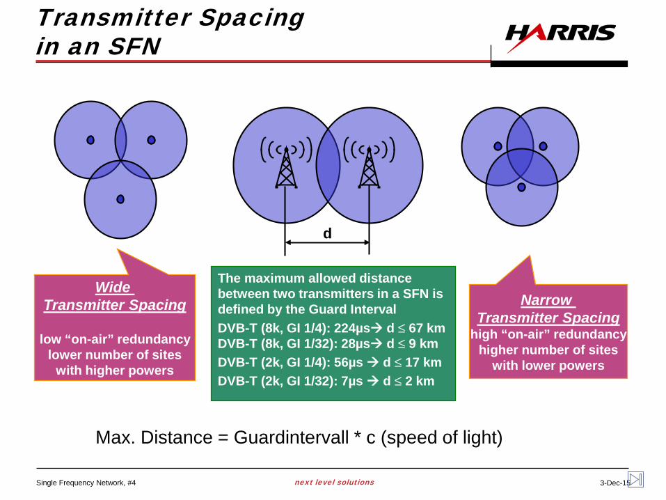
Wide Transmitter Spacing

low “on-air” redundancylower number of sites

with higher powers

Narrow Transmitter Spacing

high “on-air” redundancyhigher number of sites

with lower powers

The maximum allowed distance between two transmitters in a SFN is defined by the Guard Interval DVB-T (8k, GI 1/4): 224µs d ≤ 67 kmDVB-T (8k, GI 1/32): 28µs d ≤ 9 kmDVB-T (2k, GI 1/4): 56µs d ≤ 17 kmDVB-T (2k, GI 1/32): 7µs d ≤ 2 km

d

Max. Distance = Guardintervall * c (speed of light)

Transmitter Spacing in an SFN


MPEG-2 Multiplexer

SYNCsystem

SFN-Adapter

GPS

1 pps 10 MHz

GPS

1 pps 10 MHz

SYNCsystem

GPS

1 pps 10 MHz

TXNetworkAdapter

RXNetworkAdapter

RXNetworkAdapter

DVB-T Network Structure Using Dynamic Delay Compensation



MPEG-TS

MPEG-TS

MPEG-TS

DistributionNetwork


TXNetworkAdapter

RXNetworkAdapter

DistributionNetwork

SYNCsystem

Maximum Delay

MPEG-2 Multiplexer

SFN-Adapter


GPS

1 pps 10 MHz

GPS

1 pps 10 MHz

Maximum delay

Maximum delay: The maximum delay describes the difference in time between a specific Mega-frame leaving the SFN adapter and the corresponding COFDM Mega-frame available at the antenna output of each Transmitter in the SFN.

The maximum delay is a value adjustable in the SFN-Adapter. The set value has to be always higher than the longest actual network delay. The value is transported in each MIP


Telecom Network(Microwave, Fibre optics)

SFNAdapter

Max. Delay 700ms

500ms

400ms

Signal transmittedat the same time

Calculated TX delay time

SYNCSystem


GPS

1 pps 10 MHz

GPS

1 pps 10 MHz

SYNCSystem


GPS

1 pps 10 MHz

Signal transmittedat the same time

Transmitter Synchronisation Dynamic Delay Compensation


Synchronisation Time Stamp

Synchronisation Timestamp (STS) The synchronisation timestamp value is the difference in time between the rising edge of the 1pps Symbol and the beginning of a mega-frame M+1

1pps pulse

STS STS

M M+1 M+2

MIP

The STS is carried in the MIP of each Mega-frame.

The STS carried in the Mega-frame M describes the beginning of the Mega-frame M+1

The STS carried in the Mega-frame M+1 describes the beginning of the Mega-frame M+2

etc.


The time a frame has to be stored in the transmitter before it is sent is calculated like this:

Max. delay - actual delay= 900 ms - 350 ms = 550ms

The actual delay of the M+1 frame at the input of the Transmitter is calculated like this:

Arrival time of frame (M+1) - STS value = 650 ms - 300 ms = 350 ms

time

M M+1 M+2

650ms

SFN-Adapteroutput

Trans-mitterinput

1pps.(GPS)

Trans-mitteroutput

Adjusted max. delay = 900 ms.

The difference in time between the latest pulse of the 1pps signal and the start of the Mega-Frame

M+1 is copied into the MIP of Mega-Frame M

M M+1 M+2

max. delay = 900 ms.

M+1M-1 M

STS = 300 ms

TX delay time550 ms

Functional Description of SFN Synchronisation


SFN DVB-T2

• All transmitters in the SFN send the• same signal with SISO or MISO processing • at the same time• on the same frequency


Some specific aspects of SFN

The main feature of SFN DVB-T/T2 network is a high spectrum efficiency. A large number of programs can be broadcast on the same frequency in a local, regional or nationwide transmitter’s network.

Various modulation schemes with FFT sizes and guard intervals allow construction of SFN networks designed for different applications: from low bit-rate but robust mobile reception to the high bit-rate fixed reception for domestic and professional use.

In general, the SFN mode has many advantages but one drawback is the frequency selective fading in DVB-T or DVB-T2 network in SISO configuration. Depending on phase relationship signals may cancel each other and this will appear as a “notch” or a slope across the band.



The notch depth will depend on the relative amplitude of the receiving signals and delay.

The worst case will happen if the RX signals have the same amplitude and delay.

Measured results are shown below.

Amplitude/Delay differences between

two RX signals are “zero”Notch in the spectrum



Continued:

Variations of MER values

Variations of MER by carriers

Amplitude/Delay differences between two RX signals = 0



Continued:

Delay difference is 3us

Delay difference between two RX signals is 0.5us Delay difference is 1us

An increase of the SFN offset delay in one of two transmitters will decrease the notches and improve the signal quality of receiving signal.

Amplitude difference between two RX signals is 0 dB

Ripple in the spectrum


Practical consideration

Noise floor

Interference from TX1

TX1


TX2SFN overlap area

Distance

dBm

In the field there are many different configurations of SFN DVB-T/T2 networks but here will be considered three:-Transmitter spacing is within the safety distance for SFN with high on-air redudancy (Fig.1)-Transmitter spacing is within the safety distance for SFN with low on-air redundancy (Fig. 2)-Transmitter spacing is out of the SFN limit (Fig.3)

It is supposed that all transmitters have the same ERP (Effective Radiated Power) and the SFN offset delay.

In the middle of the SFN overlap area (dashed line) can occur the „notches“ in the spectrum

Fig. 1

Type 1.


Practical consideration

Distance

Noise floor

TX1 TX2

SFN overlap area dBm

Noise floor


TX1


TX2

SFN overlap area

Distance

dBm



Fig. 3

Fig. 2

Type 2.

Type 3.

Non-SFN Non-SFN


Problem solving

To avoid the notches in the spectrum an SFN offset delay should be introduced in one of two transmitters. This could move the problem to another location if the delay is relative small (3us…5us…)The delay should guarantee a reliable reception which will happen at the distance where the amplitude difference between two RX signals are relative large. If possible this distance should be set outside the overlap area.

Based on the propagation curves defined in the ITU Recommendation ITU-R P.370-7 (see Annex) it is possible to determine the distance and using the formula:

Delay [us] = (Distance [km] / Speed of light [km])*10

to calculate appropriate SFN offset delay.

6


Setting up of transmission site delays in the SFN

Delay: 35us

Example:

An SFN offset delay 35us will avoid the “notches” in the middle of the SFN overlap area and move this “problem” to the distance 10 km far away where the amplitude difference between two RX signals is large enough to prevent an reoccur of the notches.In general, the SFN offset delay will reduce the safety distance for SFN and could lead to the scenario 3 (see Fig. 3). This will not cause a problem if the power level between signals from TX1 and TX2 is greater than 35 dB in this Non-SFN area.

RX Spectrum


Annex

For Coverage estimation

the free-space path loss (FSPL) formula can be used given by:

where f (frequency) is in MHz and d (distance) in km,

and the propagation curves defined in the ITU Recommendation ITU-R P.370-7

Documents

Single Frequency Network Structural Aspects & … Frequency Network, #6 next level solutions 3-Dec-15 TX Network Adapter RX Network Adapter Distribution Network SYNC system Maximum