PERGAMON Mathematical and Computer Modelling 34 (2001) 511-525

MATHEMATICAL

COMPUTER MODELLING

www.elsevier.nl/locate/mcm

Single Camera Based Motion and Shape Estimation using

Extended Kalman Filtering

H. KANO Department of Information Sciences, Tokyo Denki University

Hatoyama, Hiki-Gun, Saitama 350-0394, Japan

B. K. GHOSH Department of Systems Science and Mathematics

Washington University St. Louis, MO 63130, U.S.A.

H. KANAI Nippon Telegraph and Telephone Corporation, Tokiwa 5-8-17

Urawa, Saitama 336-0001, Japan

(Received Octobei 2000; accepted December 2000)

Abstract-The problem of estimating motion and shape of a moving object has been considered from a time series of image data obtained via perspective projection. First of all, we analyze motion and shape dynamics of a planar surface undergoing rigid motion. It is shown that, for a class

of motion parameters, the shape parameters are asymptotically decoupled from the optical flow

dynamics, hence, become unobservable, asymptotically. For other choices of motion parameters, shape parameters remain asymptotically observable. We present a numerical study and compare

a recursive algorithm using an extended Kalman filter with a nonrecursive algebraic method, for estimating motion and planar surface parameters. The conclusion of the paper is that recursive

methods yield robust estimates whenever they are applicable. Algebraic estimation schemes, on the other hand, are always susceptible to noise. @ 2001 Elsevier Science Ltd. All rights reserved.

Keywords-Motion, Shape, Estimation, Filtering, Optical flow, Rigid motion.

1. INTRODUCTION

The problem of estimating motion and shape of objects under motion from their corresponding

image data observed over time is of paramount importance in various branches of engineering

and medical sciences. In general, the solution to the associated estimation problem is ill-posed

and is, therefore, quite susceptible to noise in the observed image data. In order to alleviate the

noise problem, various recursive estimation schemes have been proposed, the most important of

which is probably extended Kalman filtering, see [l]. Recently, a new implicit extended Kalman

filtering has also been studied by Soatto [2] and by Soatto, F’rezza and Perona [3]. The basic

estimation problem is described as follows.

Assume that we have a rigid surface that is undergoing a rigid motion parametrized by finitely many parameters. Assume that a set of feature points on the surface has been projected per-

08957177/01/g - see front matter @ 2001 Elsevier Science Ltd. All rights reserved. PII: SO895-7177(01)00079-6

Typeset by &&%K

512 H. KANO et al.

spectively on an image plane and that the image data has been observed over an interval of time. The problem is to simultaneously estimate the shape of the surface and the corresponding motion parameters.

In general, if the feature points are observed exactly, then the problem of computing the motion and shape parameters of a planar surface undergoing a rigid motion has been considered in the literature over the last 15 years. Many of these techniques are based on solving a set of nonlinear algebraic equations and are, therefore, nonrecursive [4-61. These algebraic methods yielded feasible results, but were far from providing an acceptable computational algorithm.

In order to obtain algorithms that are robust with respect to noisy image data, recursive algo- rithms have been introduced and studied, see [7,8]. A question that is of paramount importance is the following.

What is a suitable parametric class of motion dynamics, that could yield robust recursive algo-

rithms?

The main results of this paper are now summarized. We consider a planar surface undergoing a rigid motion and show that for a generic choice of the motion parameters, the shape parameters are asymptotically decoupled from the optical flow dynamics. This leads to the conclusion that asymptotically the shape parameters are invisible from the image data, and hence, recursive shape estimation would not be possible under perspective projection for a generic class of motion parameters. In this paper, we confirm this conclusion via simulation. We also analyze a suitably rich, nongeneric class of motion dynamics for which “shape-parameters” remain asymptotically observable. Once again, using simulation, we show how the parameters are recoverable.

2. RIGID MOTION DYNAMICS IN R3

We begin this section by considering a parametrized class of dynamics that has been studied in great detail in the literature [4,9] pertaining to the problem of estimating the motion parameters. In particular, in this paper, we would like to discuss the extent to which the parameters can be estimated using asymptotic and recursive algorithms.

In order to introduce the specific problem, let (X, Y, 2) denote a set of coordinates in R” where we consider a motion dynamics as follows:

(t\ = Lowi ‘;I’ $I (C\ + (it\,

\i] \-~2 -w3 O/ b/ \b3/

or simply,

Here,

x=

k=RX+b.

0 w1 w2

-w1 0 w3

-w2 -w3 0 1. b=

(2.1)

(2.2)

bl

0 bz . bs

(2.3)

As one can see, (2.2) is described by six motion parameters, which are, for the purpose of this paper, assumed to be time invariant. The dynamics (2.2) have been studied in the literature as a model for rigid motion and, of course, it is known classically that any rigid transformation can be represented by (2.2) if one allows the motion parameters to be time varying.

To get an insight to the geometric structure for the phase portrait of (2.2), we make the following transformation:

xi =x+CY, (2.4)

with Xi = (Xi,Yi, 21)~ and a = (~!i,az,crs)~. Differentiating (2.4), we get

it1 = k = f2Xl + (b - aa). (2.5)

Single Camera Based Motion 513

Note that the skew symmetric matrix (R) in (2.3) has rank 2 in general. Let us define

P fiImS2, (2.6)

where P is a homogeneous two-plane in R 3. We now decompose the vector b as follows:

b = bl + bp, (2.7)

where bl E P and b2 E P’. Note that the decomposition (2.7) is unique. Let us now choose a

in such a way that

Q2~y = bl.

It would follow that (2.5) reduces to

A?1 = RX1 + b2,

where b2 is an eigenvector corresponding to the eigenvalue

scalar p,

bz = Pv,

with

v = (w3, -w2, W1)T .

(2.8)

(2.9) 0. It follows that there exists a

From (2.9),(2.10), we conclude that there exists an orthogonal matrix R such that if

X2 = RXl,

with X2 = (X2, Y2, ZZ)~, we obtain

A?2 = Ax2 + 1;.

Here,

fi+; A I), 6=(%j.

and w = wf + wg + wz. Equation (2.12) can be solved easily as follows:

(2.10)

(2.11)

(2.12)

(2.13)

(2.14)

Thus, the magnitude of the vector X2 is linearly increasing to “infinity” while the direction is

asymptotically the direction of the vector (0 0 l)T in the (X2, Yz, 2~)~ coordinate. It would follow

that in coordinate (Xl, Yl, ZI)~, the asymptotic direction of the vector is along the direction of

(ws -wq ~1)~. The conclusion would be same in the coordinate system‘(X, Y, Z)T as well. Thus,

we have the foilowing theorem.

THEOREM 2.1. Consider the dynamical system (2.2) where we assume that (wl w2 w3) # 0. If

bEImR, (2.15)

then the phase portrait of (2.2) is circular and periodic with axis of rotation given by

Pv+a, (2.16)

where (Y is a vector such that Ra=b, (2.17)

and where p is an arbitrary scalar. If, on the other hand, (2.15) is not satisfied, then the

magnitude of the vector X linearly increases to infinity and

t’i% [x(t)] = [vl = [w3, --W2,4T * (2.18)

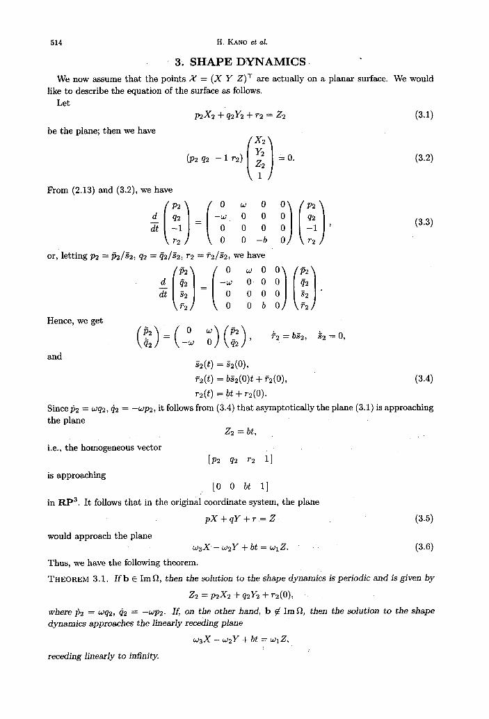
514 H. KANO et al.

’ 3. SHAPE DYNAMICS.. *

We now assume that the points X = (X Y Z)T are actually on a planar surface. We would

like to describe the equation of the surface as follows.

Let

be the plane; then we have

P2X2 +q2y2 +r2 = 22

x2

(3.1)

(P242 -1r2) yz

0

= 22

0. (3.2)

1

From (2.13) and (3.2), we have

or, letting p2 = p~/sz, qz = ~&iz/&, r2 = Fz;Z/SZ, we have

(3.3)

Hence, we get

(!!)=(_“w 5) (;), P2=bS2, sL2=0,

and 52(t) =32(O),

p2(t) = bSz(O)t + Q,(O),

r2(t) = bt + ~~(0).

(3.4)

Sincep2 = wq2, Q = -wps, it follows from (3.4) that asymptotically the plane (3.1) is approaching

the plane 22 = bt,_

i.e., the homogeneous vector

LP2 Q2 T2 11 is approaching

[0 0 bt l]

in RP3. It follows that in the original coordinate system,

pX+qY+r=Z

would approach the plane

the plane

w3X-w2Y+bt=w1Z. .’

(3.5)

(3.6)

Thus, we have the following theorem.

THEOREM 3.1. If b E ImR, then the solution to the shape dynamics is periodic and is given by

22 =p2x2 +qzyz +r2(0),

where fi2 = wqz, 42 = -wp2. If, on the other hand, b @ ImQ then the solution to the shape

dynamics approaches the linearly receding plane

w3X - w2Y + bt = wlZ,

receding linearly to infinity. i

Single Camera Based Motion 515

4. OPTICAL FLOW DYNAMICS

We now assume that the state vector (X Y ,QT is observed via perspective projection where

X 2=--, z y= ;.

Differentiating (4.1) and using (2.1), we get

k= &k--xi A i

22 =z--“z

bl b3 = (w~y+w~)-z(-w2z- w3y)+ - --2--.

z z

Since

Z=pX+qY+r,

(4.1)

(4.2)

we have 1 1-P--qY -= z r ’

Hence,

Li? =w2+w1 y+w2z2+w3xy+(c1-x3)( l- pz-qy),

where q = bJr, i = 1,2,3. Similarly, we obtain

(4.3)

(4.4)

g = w3 - WI2 + w25y + w3y2 + (c2 - c3y) (1 - pz - qy).

Equations (4.4),(4.5) denote the optical flow equation. Ix&particular, when t + 00, .

(4.5)

biw ci+x, i = 1,2,3.

Thus, we have the following theorem.

THEOREM 4.1. When b $ Im 0, the coefficients of the optical flow dynamics (4.4),(4.5) approach

the coefficients of the following dynamics:

k =w2 +wI~+w~x~+w~xY+; (bl -b3z)(wl- w3x+wzy),

$=“&--W~x+W2x~+W3y2+~ ’ (b2 - kiy) (WI- ~32 + WRY) .

If b E Im R on the other hand, the optical flow equation asymptotically is given by

(4.6)

k =w2 +w1y+w2x2+w32y+ r(t) 1 (bl - b) (1 - PX - m),

ti= w3 -w+w2~Y+w3Y2+ r(t) +2 -b3y)(l - PX-WI,

where p(t) and q(t) are periodic functions satisfj&g the Riccati equation

p = w1q - (32 - wzp” - w3pq,

Q= -w1p- w3 -w2pq- w3q2,

i=b3-brp-b2q-r(w3q+wZp).

(4.7)

(4.8)

516 H. KANO et al.

5. SIMULATION STUDIES

Simulation studies are performed focusing specific attention on whether or not (2.15) is satisfied.

Motion and shape parameters are estimated from noisy image data by employing an extended

Kalman filter. For convenience of numerical computation, the filter is designed in discrete-time

settings.

5.1. Time-Discretized Motion and Shape Dynamics

The continuous-time motion dynamics (2.2) is now discretized with sampling time T as

&c+l = A& + g. (5.1)

Here & = X(/6!‘) = (xk, Yk, zk)T, and A = [aij] and g = (gr, gs, gs)T are obtained as

A = ,Or, g = I ’ e”i(T-‘)bdT. Jo

Motion parameters are now aij and gi, i, j = 1,2,3. Then, with w = ,/w: + wi + w$ # 0, the

following relation holds:

R= & (A - AT) ’ (5.3)

where w is given by

w = +Atan2 (“yz,yr) . (5.4)

Here, A tan 2(., .) is the two-variable arctangent function (see, e.g., [lo]), and 71 and 72 are defined

as

yl = tr.A - 1, ,=$A-A’ll, (5.5)

with ]] . 1) b ein g matrix Euclidean norm. This formula can be used to compute R from A.

On the other hand, the equation of planar surface is given by

zk = Pkxk + qkyk + Tkr (5.6)

where pk, qk, and rk are the shape parameters. The shape dynamics corresponding to (4.8) is

then given [ll] as &rPk + fkzqk - A13

“+l = - A31pk + &qk - A33 ’

&lPk + h9k - A23 qk+l = -

&lPk + hwc - A33 ’

(5.7)

and

rk+l = g3 - rk - 91 (AllPk + A129k - A13) - Q2 (&oPk + &2qk - A23)

&Ple + fh9k - A33 (5.8)

Here Aij denotes the cofactor of aij of rotation matrix A.

Under perspective projection, a feature point & iS observed as a point (zk, &) on the image

plane by xk = Xk/Zk and yk = Yk/zk yielding the following optical flow dynamics.

xk+l = dl,kxk + &,kYk + dS,k

d7,kxk + dS,kyk + dg,k ’

dl,kXk + &,kYk + dS,k

“+I = h,kXk + dS,kYk + dg,k ’

(5.9)

Single Camera Based Motion 517

Here, di,]e, i = 1,2, . . . , 9, called essential parameters, are defined as

4,k = a11 - Cl,kPk,

da,k = a21 - C2,kPk,

d7,k = asi - C3,kPk,

d2,k = ‘J12 - Cl,kqk,

&,k = a22 - CP,kqk,

&,k = a32 - C3,kqk,

d3,k = ‘J13 + cl,k,

‘&,k = a23 + CZ,k,

&,k = a33,

(5.10)

and C&k, i = 1,2,3, defined by

clk=Q1 Tk ’

C2k=QZ rk ’

C3k=Q3 rk ’

(5.11)

are governed by the following recursive equations.

c, k+l = (A3lPk + A32qk - A331 Ci,k 2,

Ek , i = 1,2,3, (5.12)

where Ek = (AllPk + b2qk - A13) cl,k + (AzlPk + A22qk - A23) C2,k

+ (A31Pk + A32qk - A33) C3,k - 1.

(5.13)

5.2. Extended Kalman Filter

We are now in a position to design an extended Kalman filter (e.g., [12]). It is noted that,

theoretically [9], the drift vector g and Tk are identifiable only in the form of the ratios, namely

as Ci,k, i = 1,2,3 in (5.11). The parameters to be estimated are now a~, C&k, for i, j = 1,2,3,

and Pk, qk*

It is assumed that, at each time instant k, a set of n positions (zik, yik), i = 1,2,. . . , n

corresponding to n feature points xik, i = 1,2,. . . , n on the surface are measured. Hence, as a

state vector ok, we take

81, = (all,k&2,kr.. . , T

~33,k,Cl,k,C2,k,C3,k,~k,~kr~lk,Ylk,~~~,~nk,Ynk) , (5.14)

with & E R2n+14. The associated state equation denoted as

ok+1 = f (ok) (5.15)

follows readily from Uij,k+l = aij,k for i,j = 1,2,3, (5,12), (5.7), and (5.9).

On the other hand, let the position (zik, Yik), i = 1,2,. . . , n be observed with additive noises,

and let zk E R2n be the observation vector. Then the observation equation is given by

.zk = Hek + wk, (5.16)

where H E Ranx (2n+14) is defined by H = [0 2n,1412n]. {?_I&} is assumed to be a Gaussian white

noise with mean zero and covariance R, namely,

E {wk$} = R&l, (5.17)

where 6kl denotes Kronecker delta.

It is now a straightforward task to derive an extended Kalman filter, as summarized below.

Letting &,k and f&+-i be the estimates Of ok given the data (20, 21, . . . , zk} and {a, ~1,. . . , &__1}, respectively, the filter equation is given by

dk,k = dk,k-, + Kk [zk - Hik,k-ij , &,-I = go,

(5.18)

518 H. KANO et al.

with the Kalman gain

K,, = Pk,,&@ [H&,&1@ + RI-‘.

The error covariance matrix pklk for k&k, and Pk+,-+llk for &+llk, are then given by

Pklk = pklk-1 - IckHPkIk-1, POl-1 = co,

Pk+llk = Fkpk,kF:,

where Fk is the Jacobian matrix of f(e) evaluated at 0 = &klk, namely,

0.5 1 I

0.5 0 0.5 1 1.5 2 2.5 3 Y

Figure 1. Sample trajectory on image plane for the case 6 E ImO.

2.5 -

/

,

2-

1.5- /’

21 --\

o.I; .lj-.llh.:

0.5 ’ j 0.5 0 0.5 1 1.5 2

x

(5.19)

(5.20)

(5.21)

Figure 2. Sample trajectory on image plane for the case 6 e Im R.

Single Camera Based Motion 519

0.97

0.95’ 0 60 100 160 200 260 300 360 400 450 !

k

Figure 3. Estimated value &ll,k (solid line) and true value all (dotted line) for the csse bE Imf2.

i

1

C

6

6 50 loo 150 200 250 300 350 400 450 500

k

Figure 4. Estimation error variance (vertical axis in log scale) for all, for the csse b E ImR.

5.3. Simulation Results

We first show the motion and shape parameters used in our simulation studies. In (2.2), Sl is

set by (WI, ~2, ~3) = (-0.2,0.1, -O.l), and we consider the following two cases for b depending

on whether or not b E ImQ.

CASE 1.

b = (0.1 0.1 -0.1 )T E ImR. (5.22)

CASE 2.

b = (0.1 0.1 O.l)T $Imfi. (5.23)

520 H. KANO et al.

0 50 100 150 200 250 300 350 400 450 500 k

Figure 5. Estimated parameter Ljl,k (solid line) and true value WI (dotted line) for the case b E ImR.

0 0 50 100 150 200 250 300 350 400 450

k

Figure 6. Estimated value El,k (solid line) and true value c1.k (dotted line) for the casebEImn.

Then, with T = 0.1, the rotation matrix A is computed as

A=

i

0.9998 -0.0199 0.0101

0.0200 0.9998 -0.0099 (5.24) -0.0099 0.0101 0.9999

and the drift vector g in (5.1) as g = (0.0098 0.0101 -O.O1OO)T for Case 1 and g = (0.0099

0.0100 O.O1OO)T for Case 2. Initial values for shape parameters in (5.6) are (pa,qo,rc) =

(O.l,O.l, 2.0). The number of feature points n to be observed is assumed to be n = 3, hence, f?k E R20 in (5.15)

and zk E R6 in (5.16). The noise covariance R in (5.17) is set as R = 0~16 with cr = 0.01. Finally,

for the initial conditions in the Kalman filter, & is taken as the 20-dimensional vector with 1s in

its first, fifth, and ninth positions and OS elsewhere, and Ca = 100120.

Single Camera Based Motion 521

0 50 loo 150 200 250 300 350 400 450 500 k

Figure 7. Estimated value fik (solid line) and true value pk (dotted line) for the case

bcC352.

2.5 -

3 -

3.5 -

0 50 loo 150 200 250 300 350 400 450 500 k

Figure 8. Estimated value Ijk (solid line) and true value pk (dotted line) for the case

b@ImR.

Sample trajectories on the image plane corresponding to a feature point on the planar surface

are plotted in Figures 1 and 2 for the cases b E Im fi and b # Im fl, respectively. We may recognize

that the noises are fairly large. In the following figures, we show the estimation results where

estimated values are plotted in solid lines and true values in dotted lines for k = 0, 1, . . , ,500.

First, we present the simulation results for Case 1, i.e., the case b E ImR. As a typical example

of the estimates &j,k, i, j = 1,2,3, Figure 3 shows the plot of &ir,k. We may observe ,that &ii&

is converging to the true value ail. In fact, from the plot of the corresponding estimation error

variance in Figure 4 where vertical axis is in log scale, standard deviation of the error has been

reduced eventually to the order of lo- . * The motion parameters wi, ~2, wg in continuous-time dynamics are recovered from &j,k, i,j = 1,2,3 by (5.3)-(5.5), and the result for &,k presented in Figure 5 shows quite fast convergence. Figure 6 shows the estimate for the parameter c1.k

622 H. KANO et al.

30 -

25-

c -,20-

0 50 loo 150 200 250 300 350 400 450 500 k

Figure 9. ‘Ikue vdue of fk for the case b $! ImC2.

15 20 tru value of rk

Figure 10. Normalized estimation error s& plotted-against rk with k as the parameter

for the case b g’ Im 0.

in (5.12), and we observe that accurate tracking has been achieved. We confirm that the associ-

ated error variance has decreased to the order of 10S7. The estimate of the shape parameter pk

is plotted in Figure 7. The performance is not quite satisfactory, especially in the valley portions

of the plot which arise periodically and correspond to a large, value of rk. This phenomenon

becomes more evident in Case 2 as we will see shortly.

Next, we consider Case 2 in (5.23). Equally good performance as in Case 1 was observed for the estimation of aij, c+,k, and WC, i, j = 1,2,3. On the other hand, as we see in Figure 8, the

performance ‘for shape parameter pk is far from satisfactory. From Figures 8 and 9, where true value of rk is plotted, we see that the error is large whenever the value of flk’ is large.

Single Camera Baeed Motion 523

20

15

cj 10

5

0

I I

51 0 50 100 150 200 250 300 350 400 450 500

time

Figure 11. Estimated parameter G1.k by algebraic method for the case b E Imn.

150 200 250 time

300

Figure 12. Estimated value Ijk by algebraic method for the cese b E Im R.

Such a phenomenon becomes more evident from Figure 10, where the following normalized

estimation error ek for pk and qk,

d (Ijk -pk12 + (#k -Pk)? Ek =

J_ (5.25)

is plotted against rk with k bemg the parameter. According to Theorem 4.1, the trend of rk

recedes to infinity linearly with time, and eventually pk and qk are decoupled from optical flow equation. This implies that the estimation becomes worse and worse as time proceeds:

Finally, for the sake of com&rison, we computed the motion and shape parameters by existing

method based on a solution of a .set .of nonlinear algebraic equations [4]. Since this method

requires position and velocity data for at least four feature points, we took a fourth feature point

524 H. KANO et al.

additionally on the planar surface to result in the data (Q, yirc) and (kik, &) for i = 1,2,3,4.

Thus, we have a total of 16 observation data at each time instant k, to which noises with the

same statistical properties as in the previous experiments are added. As the typical examples,

&l,k and ?jk are shown in Figures 11 and 12, respectively. Note that this method is known to

yield two sets of motion and shape parameters, one of which corresponds to the true parameters

and the other gives ‘fake’ parameters. In these figures, we plotted the set that corresponds to the

true one, which we know from a pre-experiment without noises. Comparing Figures 11 and 12,

respectively, with Figures 5 and 7, it is obvious that the algebraic method is highly sensitive to

additive observation noises.

6. CONCLUDING REMARKS

We considered the problem of estimating motion and shape parameters of moving rigid body

from noisy image data under perspective projection. Such a motion is described by the equation

with skew symmetric matrix R, which is widely used in the theory of machine vision.

First, by introducing suitable coordinate transformations, we clarified asymptotic behavior of

motions depending on whether or not the drift vector b is in ImR. In particular, if b E ImSt,

the motion was shown to be circular and periodic around certain axis of rotation. On the other

hand, if b # Ima, then the body is proved to be receding to infinity linearly in time in the

direction of the eigenvector of fl corresponding to zero eigenvalue. The shape parameters are

then asymptotically decoupled from optical flow dynamics and are asymptotically invisible from

the image data.

Secondly, the results of such analyses were confirmed by computer simulation studies. Here,

we employed the extended Kalman filter assuming that the image data is corrupted with additive

observation noise. In both cases, b E ImS2 and b $i ImR, motion parameters were recovered

successfully with sufficient accuracy. On the other hand, the performance for shape parameters

becomes poor whenever the rigid body becomes far from the camera, which always is the case if

b @Ima.

As we have seen from the simulation results, the Kalman filter employed here for estimating

motion and shape parameters provides various advantages over the conventional nonrecursive

method based on solutions of nonlinear algebraic equations. It is naturally more robust to noises

in image data and the same is expected to modelling errors in equation of motion. Since we

formulated the identification problem as the state estimation problem for dynamical system, the

scheme is recursive, and velocity in image data is not required, unlike the nonrecursive algebraic

method.

REFERENCES

1. L. Matthies, T. Kanade and R. Szeliski, Kalman filter-based algorithms for estimating depth from image sequences, Int. J. Comput. Vision 3, 209-236. (1989).

2. S. Soatto, A geometric framework for dynamic vision, Ph.D. Thesis, California Institute of Technology

(1996). 3. S. Soatto, R. Frezza and P. Perona, Motion estimation via dynamic vision, IEEE ‘l+ansactions on Automatic

Control 41 (1996). 4. K. Kanatani, Group-Theoretical Methods in Image Understanding, Springer-Verlag, (1990).

5. M. Subbarao and A.M. Waxman, On the uniqueness of image flow solutions for planar surfaces in motion, Technical Report 114, University of Maryland, College Park, Center for Automation Research (1985).

6. A.M. Wsxman and S. Ullman, Surface structure and 3-D motion from image flow: Kinematic analysis,

Intentational .I. Robotics Research 4, 72-94 (1985). 7. M. Jankovic and B.K. Ghosh, Visually guided ranging from observations of points, lines and curves via an

identifier based nonlinear observer, Syst. Con&. Lett. 25, 63-73 (1995).

8. X. Matveev, X. Hu, R. F’rezza and H. Rehbinder, Observers for systems with implicit output, IEEE Zkans- actions on Automatic Control 45 (l), 168-173 (2000).

9. B.K. Ghosh and E.P. Loucks, A perspective theory for motion and shape estimation in machine vision, SIAM J. Control and Optimization 33, 1530-1559 (1995).

Single Camera Based Motion 525

10. J.J. Craig, Introduction to Robotics: Mechanics and Control, Second Edition, Addison-Wesley, (1989). 11. E.P. Loucks, A perspective systems approach to motion and shape estimation in machine vision, Ph.D.

Thesis, Washington University (1994). 12. B.D.O. Anderson and J.B. Moore, Optimal Filtering, Prentice-Hall, (1979).