Three-state Extended Kalman Filter for Mobile Robot ...kom.aau.dk/group/05gr999/reference_material/filtering/eKf-3state.pdf · Three-state Extended Kalman Filter for Mobile Robot

Three-state Extended Kalman Filter for MobileRobot Localization

Evgeni [email protected]

Martin [email protected]

April 12, 2002

Summary

This report describes the application of an extended Kalman filter to localiza-tion of a golf course lawn mower using fiber-optic gyroscope (FOG), odometry,and machine vision sensors. The two machine vision cameras were used toextract angular measurements from the previously surveyed artificial ground-level markers on the course. The filter showed an average 0.352 m Cartesianerror with a standard deviation of 0.296 m in position estimation and a meanerror of 0.244o and standard deviation of 3.488o in heading estimation. The er-rors were computed with respect to the existing high-performance localizationsystem.

1 Introduction

For an autonomous lawn mower to be used on a golf course its navigation sys-tem must provide accuracy and robustness to assure precision of the resultingmowing pattern. The mower state - its position and orientation in real time - isobtained by combining the available internal and external sensory informationusing an Extended Kalman Filter (EKF).

The internal sensor set consists of front wheel odometers[3] and a fiberoptic gyroscope (FOG)[4], the external, absolute sensing is currently achievedby 2 cm accuracy NovAtel ProPack DGPS[5]. The internal and the absolutepositioning information is fused in real time by an extended Kalman filter forlocalization and control of the mower. The existing DGPS high-performancelocalization system maintained 97% tracking error below a target value of10 cm [7], and is used as a ground truth. At the same time the high cost ofDGPS and its dependence on good satellite visibility calls for an alternativeabsolute localization system.

Absolute positioning based on passive or active landmarks could replacethe high-cost DGPS. In addition such a system could also provide reliable

1

2 IMAGE PROCESSING AT CMU 2

absolute positioning in places where the GPS signal is degraded or unavailable.A vision-based passive marker detection was implemented as an alternative toDGPS absolute localization. The local marker approach is general, so theresults of the experiment will estimate the localization accuracy obtainable bya marker-based system irrespective of the actual hardware implementation.

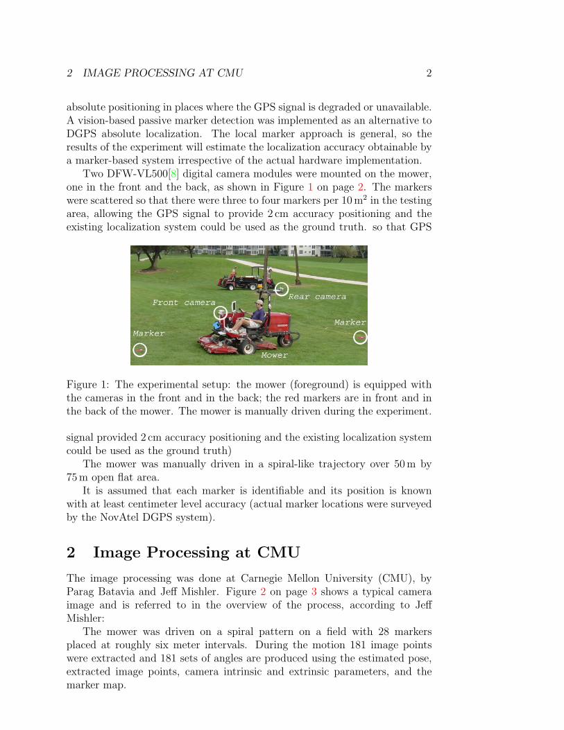
Two DFW-VL500[8] digital camera modules were mounted on the mower,one in the front and the back, as shown in Figure 1 on page 2. The markerswere scattered so that there were three to four markers per 10 m2 in the testingarea, allowing the GPS signal to provide 2 cm accuracy positioning and theexisting localization system could be used as the ground truth. so that GPS

Figure 1: The experimental setup: the mower (foreground) is equipped withthe cameras in the front and in the back; the red markers are in front and inthe back of the mower. The mower is manually driven during the experiment.

signal provided 2 cm accuracy positioning and the existing localization systemcould be used as the ground truth)

The mower was manually driven in a spiral-like trajectory over 50 m by75 m open flat area.

It is assumed that each marker is identifiable and its position is knownwith at least centimeter level accuracy (actual marker locations were surveyedby the NovAtel DGPS system).

2 Image Processing at CMU

The image processing was done at Carnegie Mellon University (CMU), byParag Batavia and Jeff Mishler. Figure 2 on page 3 shows a typical cameraimage and is referred to in the overview of the process, according to JeffMishler:

The mower was driven on a spiral pattern on a field with 28 markersplaced at roughly six meter intervals. During the motion 181 image pointswere extracted and 181 sets of angles are produced using the estimated pose,extracted image points, camera intrinsic and extrinsic parameters, and themarker map.

2 IMAGE PROCESSING AT CMU 3

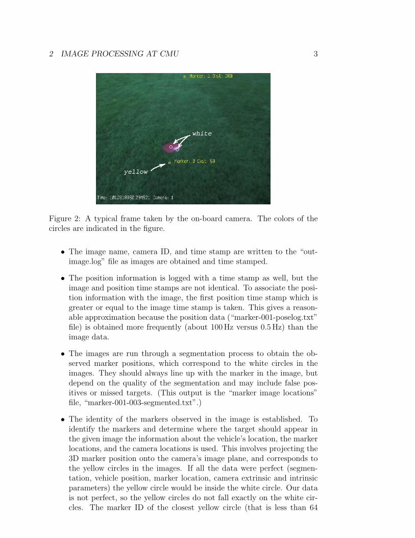
Figure 2: A typical frame taken by the on-board camera. The colors of thecircles are indicated in the figure.

• The image name, camera ID, and time stamp are written to the “out-image.log” file as images are obtained and time stamped.

• The position information is logged with a time stamp as well, but theimage and position time stamps are not identical. To associate the posi-tion information with the image, the first position time stamp which isgreater or equal to the image time stamp is taken. This gives a reason-able approximation because the position data (“marker-001-poselog.txt”file) is obtained more frequently (about 100 Hz versus 0.5 Hz) than theimage data.

• The images are run through a segmentation process to obtain the ob-served marker positions, which correspond to the white circles in theimages. They should always line up with the marker in the image, butdepend on the quality of the segmentation and may include false pos-itives or missed targets. (This output is the “marker image locations”file, “marker-001-003-segmented.txt”.)

• The identity of the markers observed in the image is established. Toidentify the markers and determine where the target should appear inthe given image the information about the vehicle’s location, the markerlocations, and the camera locations is used. This involves projecting the3D marker position onto the camera’s image plane, and corresponds tothe yellow circles in the images. If all the data were perfect (segmen-tation, vehicle position, marker location, camera extrinsic and intrinsicparameters) the yellow circle would be inside the white circle. Our datais not perfect, so the yellow circles do not fall exactly on the white cir-cles. The marker ID of the closest yellow circle (that is less than 64

3 DISCRETE EXTENDED KALMAN FILTER 4

pixels away from the white circle) is associated with this image observa-tion. (This step can be eliminated if we have barcodes or other meansof performing this data association.)

• If there is a successful match, the angles to this marker are computed andstored along with the time stamp in the “Marker angles” file, “marker-001-003-angles.txt”.

The data from “Marker angles” file is used as measurement input in theExtended Kalman Filter algorithm.

3 Discrete Extended Kalman Filter

The discrete Extended Kalman Filter [2] was used to fuse the internal positionestimation and external measurements to the markers. The following are thegeneral discrete Extended Kalman Filter [6] equations particular realizationsof which for our system are given in the Subsection 3.1.

The general nonlinear system (Equation 1) and measurement (Equation 2)where xk and zk represent the state and measurement vectors at time instantk, f(·) and h(·) are the nonlinear system and measurement functions, uk isthe input to the system, wk−1, γk−1 and vk−1 are the system, input andmeasurement noises:

xk = f(xk−1,uk; wk−1,γk−1) (1)

zk = h(xk; vk−1) (2)

removing the explicit noise descriptions from the above equations and repre-senting them in terms of their probability distributions, the state and mea-surement estimates are obtained:

xk = f(xk−1,uk,0,0) (3)

zk = h(xk,0) (4)

The system, input and measurement noises are assumed to be Gaussian withzero mean and are represented by their covariance matrices Q, Γ, and R:

p(w) = N(0,Q) (5)

p(γ) = N(0,Γ) (6)

p(v) = N(0,R) (7)

The Extended Kalman Filter predicts the future state of the system x−kbased on the available system model f(·) and projects ahead the state errorcovariance matrix P−k using the time update equations:

x−k = f(xk−1,uk,0,0) (8)

P−k = AkPk−1ATk + BkΓk−1B

Tk + Qk−1 (9)


Once measurements zk become available the Kalman gain matrix Kk is com-puted and used to incorporate the measurement into the state estimate xk.The state error covariance for the updated state estimate Pk is also computedusing the following measurement update equations:

Kk = P−k HTk (HkP

−k HT

k + Rk)−1 (10)

xk = x−k + Kk(zk − h(x−k ,0)) (11)

Pk = (I−KkHk)P−k (12)

Where I is an identity matrix and system (A), input (B), and measurement(H) matrices are calculated as the following Jacobians of the system (f(·)) andmeasurement (h(·)) functions:

A[i,j] =∂f[i]

∂x[j]

(x−k ,uk,0,0) (13)

B[i,j] =∂f[i]

∂u[j]

(x−k ,uk,0,0) (14)

H[i,j] =∂h[i]

∂x[j]

(x−k ,0) (15)

3.1 Mower System Modeling

The mower’s planar Cartesian coordinates (x, y) and heading (Φ) describe poseof the mower and are used as the state variables of the Kalman filter. Thewheels encoder and the FOG measurements are treated as inputs to the system.The angles to the markers are treated as the measurements. The mower ismodeled by the following kinematic equations representing the position of themid-axis (x, y) and the orientation in the global frame (Φ) [9].

fx = xk+1 = xk + ∆Dk · cos(Φk +∆Φk

2) (16)

fy = yk+1 = yk + ∆Dk · sin(Φk +∆Φk

2) (17)

fΦ = Φk+1 = Φk + ∆Φk (18)

Where ∆Dk is the distance travelled by the mid-axis point given the valuesthat the right and the left wheels have travelled, ∆DkR and ∆DkL respectively:

∆Dk =∆DkR + ∆DkL

2(19)

The incremental change in the orientation ∆Φk,can be obtained from odometrygiven the effective width of the mower b:

∆Φk =∆DkR −∆DkL

b(20)


Thus the system state vector may be written as xk = [xk yk Φk]T , the input

vector as uk = [∆DkL ∆DkR]T and the system function f(x) = [fx fy fΦ]T

where the function components are represented by the Equations (16 to 18).The system (Ak) and input (Bk) Jacobians for our system are given below:

Ak =

∂fx∂xk

∂fx∂yk

∂fx∂Φk

∂fy∂xk

∂fy∂yk

∂fy∂Φk

∂fΦ

∂xk

∂fΦ

∂yk

∂fΦ

∂Φk

xk

=

1 0 −∆Dk · sin(Φk + ∆Φk2

)0 1 ∆Dk · cos(Φk + ∆Φk

2)

0 0 1

xk

(21)

Bk =

∂fx

∂∆DkL

∂fx∂∆DkR

∂fy∂∆DkL

∂fy∂∆DkR

∂fΦ

∂∆DkL

∂fΦ

∂∆DkR

xk

(22)

=

12

cos(Φk + ∆Φk2

) + ∆Dk2b

sin(Φk + ∆Φk2

) 12

cos(Φk + ∆Φk2

)− ∆Dk2b

sin(Φk + ∆Φk2

)12

sin(Φk + ∆Φk2

)− ∆Dk2b

cos(Φk + ∆Φk2

) 12

sin(Φk + ∆Φk2

) + ∆Dk2b

cos(Φk + ∆Φk2

)−1/b 1/b

xk

my

D∆

mx

Bx By( , )

xB

yB− y− x

____( )

∆DR

∆DL

α

x

y

arctan

B

d

ΦM(x,y)

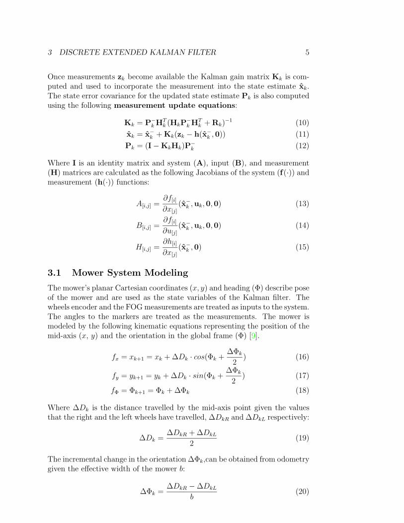
Figure 3: The system schematic (the bird’s eye view.) The blocks representthe mower wheels and the concentric circles represent a marker.

The azimuth αi with respect to the mower x-axis and elevation ηi withrespect to the mower x−y plane (observed from the mid-axis point at the dis-tance µ form the ground-plane) angles to the i-th marker obtained from thevision at a time instant k can be related to the current system state variablesxk, yk, and Φk as follows:

αi = hαi(xk) = arctan(yBi − ykxBi − xk

)− Φk (23)

ηi = hηi(xk) = − arctan(µ/di(xk)) (24)

di(xk) =√

(xBi − xk)2 + (yBi − yk)2


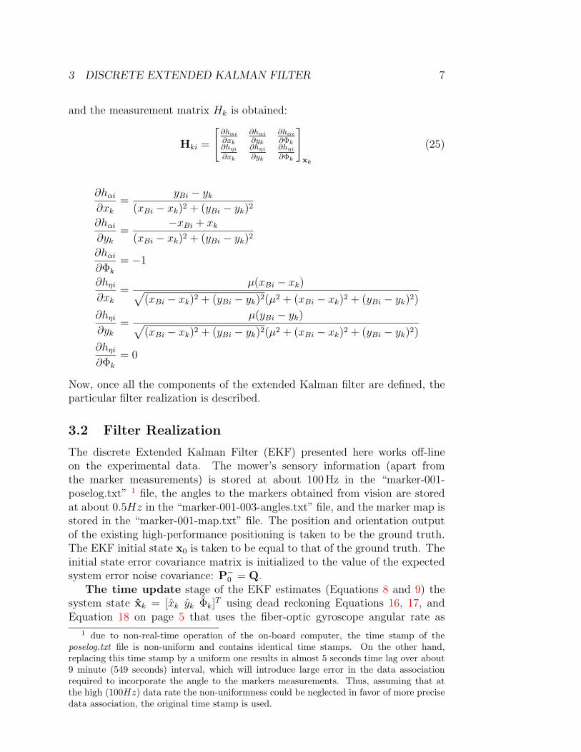
and the measurement matrix Hk is obtained:

Hki =

[∂hαi∂xk

∂hαi∂yk

∂hαi∂Φk

∂hηi∂xk

∂hηi∂yk

∂hηi∂Φk

]xk

(25)

∂hαi∂xk

=yBi − yk


∂hαi∂yk

=−xBi + xk


∂hαi∂Φk

= −1

∂hηi∂xk

=µ(xBi − xk)√

(xBi − xk)2 + (yBi − yk)2(µ2 + (xBi − xk)2 + (yBi − yk)2)

∂hηi∂yk

=µ(yBi − yk)√

(xBi − xk)2 + (yBi − yk)2(µ2 + (xBi − xk)2 + (yBi − yk)2)

∂hηi∂Φk

= 0

Now, once all the components of the extended Kalman filter are defined, theparticular filter realization is described.

3.2 Filter Realization

The discrete Extended Kalman Filter (EKF) presented here works off-lineon the experimental data. The mower’s sensory information (apart fromthe marker measurements) is stored at about 100 Hz in the “marker-001-poselog.txt” 1 file, the angles to the markers obtained from vision are storedat about 0.5Hz in the “marker-001-003-angles.txt” file, and the marker map isstored in the “marker-001-map.txt” file. The position and orientation outputof the existing high-performance positioning is taken to be the ground truth.The EKF initial state x0 is taken to be equal to that of the ground truth. Theinitial state error covariance matrix is initialized to the value of the expectedsystem error noise covariance: P−0 = Q.

The time update stage of the EKF estimates (Equations 8 and 9) thesystem state xk = [xk yk Φk]

T using dead reckoning Equations 16, 17, andEquation 18 on page 5 that uses the fiber-optic gyroscope angular rate as

1 due to non-real-time operation of the on-board computer, the time stamp of theposelog.txt file is non-uniform and contains identical time stamps. On the other hand,replacing this time stamp by a uniform one results in almost 5 seconds time lag over about9 minute (549 seconds) interval, which will introduce large error in the data associationrequired to incorporate the angle to the markers measurements. Thus, assuming that atthe high (100Hz) data rate the non-uniformness could be neglected in favor of more precisedata association, the original time stamp is used.


input independent of odometry. The covariance matrix of the prior estimateis calculated by the formula:

P−k = AkPk−1ATk + σ2

γBkBTk + Q (26)

where σ2γ is the the input noise variance (the encoders are assumed to have

the same noise variance), and Q — the 3×3 covariance matrix of the systemnoise is taken to be time-invariant.

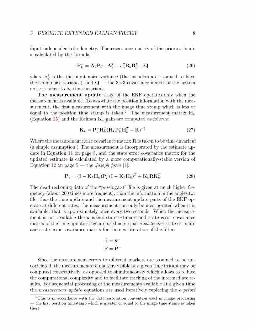
The measurement update stage of the EKF operates only when themeasurement is available. To associate the position information with the mea-surement, the first measurement with the image time stamp which is less orequal to the position time stamp is taken.2 The measurement matrix Hk

(Equation 25) and the Kalman Kk gain are computed as follows:

Kk = P−k HTk (HkP

−k HT

k + R)−1 (27)

Where the measurement noise covariance matrix R is taken to be time-invariant(a simple assumption.) The measurement is incorporated by the estimate up-date in Equation 11 on page 5, and the state error covariance matrix for theupdated estimate is calculated by a more computationally-stable version ofEquation 12 on page 5 — the Joseph form [1]:

Pk = (I−KkHk)P−k (I−KkHk)

T + KkRKTk (28)

The dead reckoning data of the “poselog.txt” file is given at much higher fre-quency (about 200 times more frequent), than the information in the angles.txtfile, thus the time update and the measurement update parts of the EKF op-erate at different rates: the measurement can only be incorporated when it isavailable, that is approximately once every two seconds. When the measure-ment is not available the a priori state estimate and state error covariancematrix of the time update stage are used as virtual a posteriori state estimateand state error covariance matrix for the next iteration of the filter:

x = x−

P = P−

Since the measurement errors to different markers are assumed to be un-correlated, the measurements to markers visible at a given time instant may becomputed consecutively, as opposed to simultaneously which allows to reducethe computational complexity and to facilitate tracking of the intermediate re-sults. For sequential processing of the measurements available at a given timethe measurement update equations are used iteratively replacing the a priori

2This is in accordance with the data association convention used in image processing— the first position timestamp which is greater or equal to the image time stamp is takenthere.

4 LOCALIZATION SIMULATIONS 9

values of the state estimate and its error covariance matrix by the updatedvalues after each iteration:

x− = x

P− = P

4 Localization Simulations

The filter was used to estimate the mower state x (position and orientation inplanar motion) by fusing the odometry, gyroscope, and the angle informationfrom the absolute marker detection. The algorithm was run on the experi-mental as well as on the simulated ideal data that would have been obtainedif the measurements had been perfect.

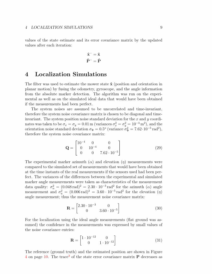
The system noises are assumed to be uncorrelated and time-invariant,therefore the system noise covariance matrix is chosen to be diagonal and time-invariant. The system position noise standard deviation for the x and y coordi-nates was taken to be σx = σy = 0.01 m (variances σ2

x = σ2y = 10−4 m2), and the

orientation noise standard deviation σΦ = 0.5o (variance σ2Φ = 7.62·10−5 rad2),

therefore the system noise covariance matrix:

Q =

10−4 0 00 10−4 00 0 7.62 · 10−5

(29)

The experimental marker azimuth (α) and elevation (η) measurements werecompared to the simulated set of measurements that would have been obtainedat the time instants of the real measurements if the sensors used had been per-fect. The variances of the differences between the experimental and simulatedmarker angle measurements were taken as characteristics of the measurementdata quality: σ2

α = (0.048 rad)2 = 2.30 · 10−3 rad2 for the azimuth (α) anglemeasurement and σ2

η = (0.006 rad)2 = 3.60 · 10−5 rad2 for the elevation (η)angle measurement; thus the measurement noise covariance matrix:

R =

[2.30 · 10−3 0

0 3.60 · 10−5

](30)

For the localization using the ideal angle measurements (flat ground was as-sumed) the confidence in the measurements was expressed by small values ofthe noise covariance entries:

R =

[1 · 10−12 0

0 1 · 10−12

](31)

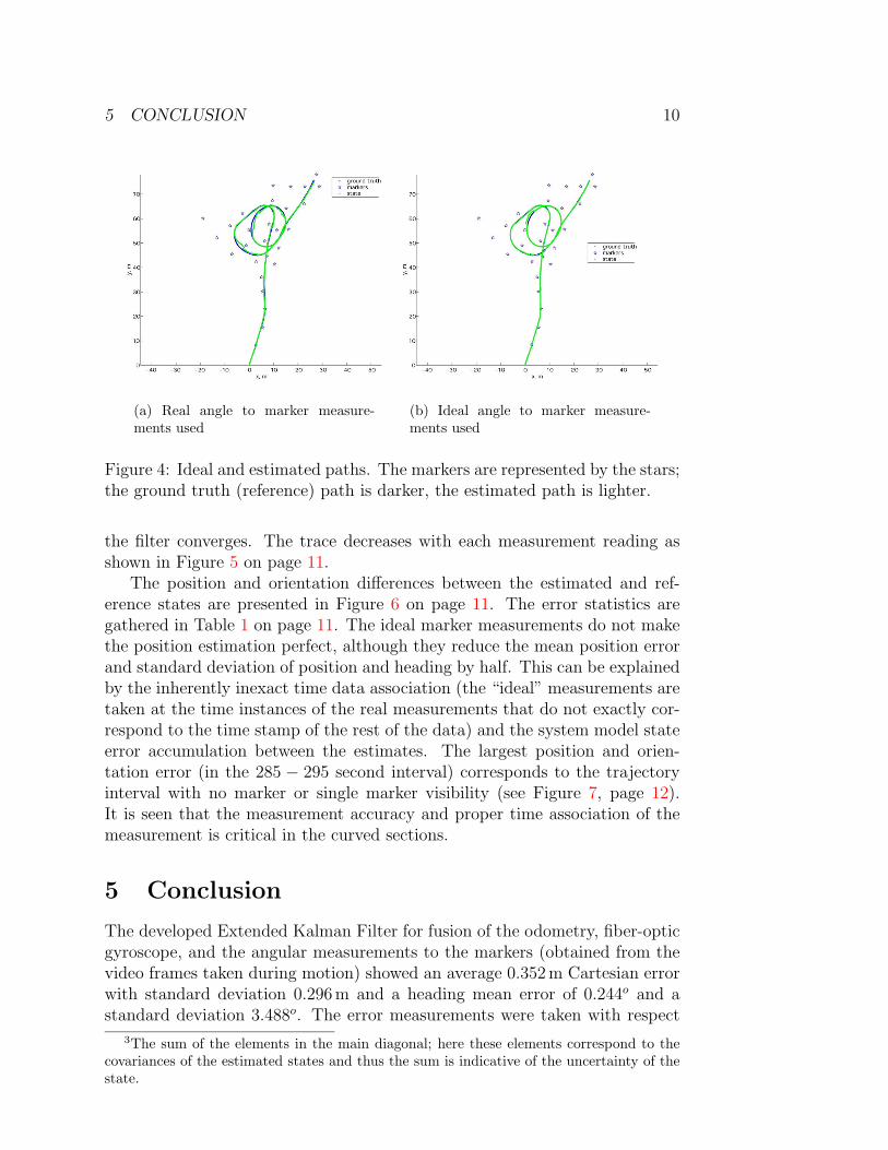
The reference (ground truth) and the estimated position are shown in Figure4 on page 10. The trace3 of the state error covariance matrix P decreases as

5 CONCLUSION 10

(a) Real angle to marker measure-ments used

(b) Ideal angle to marker measure-ments used

Figure 4: Ideal and estimated paths. The markers are represented by the stars;the ground truth (reference) path is darker, the estimated path is lighter.

the filter converges. The trace decreases with each measurement reading asshown in Figure 5 on page 11.

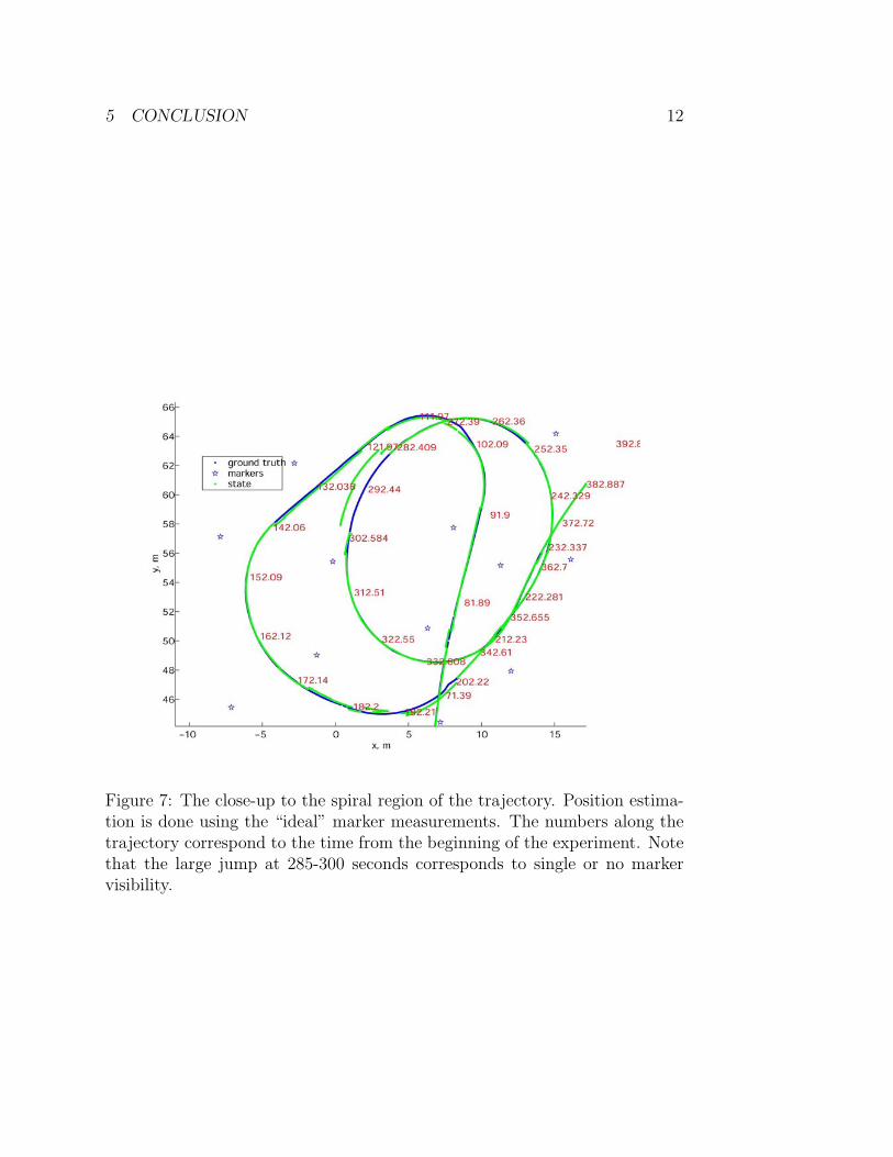
The position and orientation differences between the estimated and ref-erence states are presented in Figure 6 on page 11. The error statistics aregathered in Table 1 on page 11. The ideal marker measurements do not makethe position estimation perfect, although they reduce the mean position errorand standard deviation of position and heading by half. This can be explainedby the inherently inexact time data association (the “ideal” measurements aretaken at the time instances of the real measurements that do not exactly cor-respond to the time stamp of the rest of the data) and the system model stateerror accumulation between the estimates. The largest position and orien-tation error (in the 285 − 295 second interval) corresponds to the trajectoryinterval with no marker or single marker visibility (see Figure 7, page 12).It is seen that the measurement accuracy and proper time association of themeasurement is critical in the curved sections.

5 Conclusion

The developed Extended Kalman Filter for fusion of the odometry, fiber-opticgyroscope, and the angular measurements to the markers (obtained from thevideo frames taken during motion) showed an average 0.352 m Cartesian errorwith standard deviation 0.296 m and a heading mean error of 0.244o and astandard deviation 3.488o. The error measurements were taken with respect

3The sum of the elements in the main diagonal; here these elements correspond to thecovariances of the estimated states and thus the sum is indicative of the uncertainty of thestate.

5 CONCLUSION 11



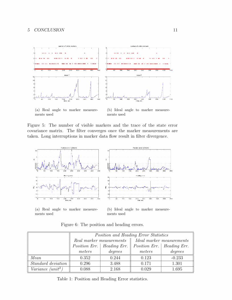
Figure 5: The number of visible markers and the trace of the state errorcovariance matrix. The filter converges once the marker measurements aretaken. Long interruptions in marker data flow result in filter divergence.



Figure 6: The position and heading errors.

Position and Heading Error StatisticsReal marker measurements Ideal marker measurements

Position Err. Heading Err. Position Err. Heading Err.meters degrees meters degrees

Mean 0.352 0.244 0.123 -0.233Standard deviation 0.296 3.488 0.171 1.301Variance (unit2) 0.088 2.168 0.029 1.695

Table 1: Position and Heading Error statistics.

5 CONCLUSION 12

Figure 7: The close-up to the spiral region of the trajectory. Position estima-tion is done using the “ideal” marker measurements. The numbers along thetrajectory correspond to the time from the beginning of the experiment. Notethat the large jump at 285-300 seconds corresponds to single or no markervisibility.

6 ACKNOWLEDGEMENTS 13

to the ground truth trajectory. The filter performance can be improved by:

• On line adjustment of the system (Qk) and measurement (Rk) covariancematrices based on the statistical properties of the incoming data.

• Extending the state of the filter to include the translational and rota-tional velocities.

• Improved real time data correlation.

• Increased external measurement data frequency.

• Improved external data precision.

6 Acknowledgements

The authors would like to thank the CMU team (Sanjiv Singh, Jeff Mishler,Parag Batavia, and Stephan Roth) for taking the data, processing, and pro-viding us with the data that went into this report. We also thank Dana Lonnfor sponsoring this work and making the trip to Palm Aire possible.

References

[1] Introduction to random signals and applied Kalman filtering: with MAT-LAB exercises and solutions, chapter 6.6, page 261. John Wiley Sons,Inc., third edition, 1997.

[2] Ph. Bonnifait and G. Garcia. ”A Multicensor Localization Algorithm forMobile Robots and its Real-Time Experimental Validation”. In Proc. ofthe IEEE International Conference on Robotics and Automation, pages1395–1400, Minneapolis, Minnesota, April 1996. IEEE.

[3] Dynaher Corporation, http://dynapar-encoders.com. Dynapar encoder se-ries H20 data sheet.

[4] KVH, http://www.kvh.com/Products/Product.asp?id=39. KVH2060 datasheet, 2000.

[5] NovAtel Inc., http://www.novatel.com/Documents/Papers/Rt-2.pdf. No-vAtel ProPack data sheet, 2000.

[6] P. Y. C. Hwang R. G. Brown. Introduction to random signals and ap-plied Kalman filtering: with MATLAB exercises and solutions. John WileySons, Inc., third edition, 1997.

[7] Stephan Roth, Parag Batavia, and Sanjiv Singh. Palm Aire Data Analysis.report, February 2002.

A MATLAB CODE LISTING 14

[8] Sony, http://www.sony.co.jp/en/Products/ISP/pdf/catalog/DFWV500E.pdf.Sony DFW-VL500 Digital Camera Module data sheet.

[9] C. Ming Wang. “localization estimation and uncertainty analysis for mobilerobots”. In IEEE Int. Conf. on Robotics and Automation, Philadelphia,April 1988.

A MATLAB Code Listing

% this is an extended Kalman filter driver script

% with sequential measurements incorporation.

switch 1

case 1

clear all

% Load the input files:

%========================================================================

positionLog_o =load(’marker-001-poselog.txt’);

% [timeStamp, MarkerID, azimuth, inclination, vehSpeed, headingRate; ...]

finalMarkerLog =load(’marker-001-003-angles.txt’);

%finalMarkerLog =load(’FinalMarkerLog’);

%MarkerMap file: [markerID, markerX, markerY; ...]

markerMap =load(’marker-001-map.txt’);

%========================================================================

case 2

clear state

end %switch

bgn=10464; % first element of the positionLog to be considered;

endd=bgn+10000;

positionLog=positionLog_o(bgn:end,:);

% get phi within +/- 2pi range (wrap)

positionLog(:,21)=mod(positionLog(:,21),sign(positionLog(:,21))*2*pi);

%hight of the reference point of the mower.

h=0.226;

% clock (generate times at 0.01 sec for the length of the experiment)

%========================================================================

switch 2 % 1) 0.01 sec time stamp. 2) original time stamp. 3) equalized time step.

case 1

dT=0.01;

time=0:dT:dT*(size(positionLog,1)-1);

timePosLog=time’+positionLog(1,3);

case 2


dT=0.01;

timePosLog=positionLog(:,3);

case 3

dT=(positionLog(end,3)-positionLog(1,3))/size(positionLog,1);

timePosLog=0:dT:dT*(size(positionLog,1)-1);

timePosLog=timePosLog+positionLog(1,3);

end %switch

timeMarker=finalMarkerLog(:,1);

%========================================================================

b=1.41; %b=1.65-0.24; % mower effective width (Hal)

% Initialize the Kalman filter:

%========================================================================

%enter loop with prior state estimate and its error covariance

%x(0)projected or prior; supplied form the driver script.

%P(0)its error covariance; supplied form the driver script.

% Initial state guess:[xM; yM; Phi];

initHead=mean(positionLog(1+1:100,21));

initHead=mod(initHead,sign(initHead)*2*pi); % get phi within +/- 2pi range (wrap)

x=[positionLog(1,19);

positionLog(1,20);

initHead];

PhiOdom=initHead;

dPhiOdom=0;

% System noise covariance:

Q11=1e-4*1.00;

Q22=1e-4*1.00;

Q33=7.62e-5*1.00;

Q=diag([Q11,Q22,Q33]);

% Error covariance matrix:

P_initial=Q;

%P_initial=diag([1e-4,1e-4,1e-4]);

traceP_initial=trace(P_initial);

traceResetValue=traceP_initial*0.5;

P=P_initial;

% Build the measurement error covariance martix:

azimuthCov=0.048^2;

inclinCov=0.006^2;

singleSensorCov=[azimuthCov inclinCov];

R=[];

R=diag(singleSensorCov);


varIn=1e-4; % input noise covariance

%========================================================================

numOfVisibleMarkers=zeros(size(positionLog,1),1);

msrmtCnt=0;

for i=1:size(positionLog,1) %main

% store state

state(:,1,i)=x;

%========================================================================

% input:

dDl=positionLog(i,4); % [m]

dDr=positionLog(i,5); % [m]

dPhiFOG=positionLog(i,9); % [rad/sec]

%========================================================================

%===========================================================================

%the Kalman filter

% The state vector:

xM=x(1);

yM=x(2);

Phi=x(3);

dD=(dDl+dDr)/2;

%===========================================================================

% TIME UPDATE EQUATIONS (predict)

% EKF time update equations:

%x(k+1)project ahead=f(x(k)estim updated w meas);

%P(k+1)project ahead=A(k)*P(k)*A(k)’+Q(k);

argmnt=Phi+dPhiFOG/2*dT;

x(1)=xM+dD*cos(argmnt);

x(2)=yM+dD*sin(argmnt);

x(3)=Phi+dPhiFOG*dT;

x(3)=mod(x(3),sign(x(3))*2*pi); % get phi within +/- 2pi range (wrap)

% Build the system matrix A:

A=eye(3,3);

%A=zeros(3,3);

A(1,3)=-dD*sin(argmnt); A(2,3)=dD*cos(argmnt);

% Build the input matrix B:

cPhi=0.5*cos(argmnt); dDs=dD/2/b*sin(argmnt);

sPhi=0.5*sin(argmnt); dDc=dD/2/b*cos(argmnt);

B(1,1)=cPhi+dDs; B(1,2)=cPhi-dDs;

B(2,1)=sPhi-dDc; B(2,2)=sPhi+dDc;

B(3,1)=-1/b; B(3,2)=1/b;

P=A*P*A’+varIn*B*eye(2,2)*B’+Q;


%P=A*P+P*A’+Q;

%===========================================================================

%===========================================================================

% Now, if a measurement is available - incorporate it:

if ~isempty(finalMarkerLog) % check if markers exist

% find the measurements corresponding to the current time instance:

% according to CMU association: t_posLog>=t_marker

measurementEntries=find(timeMarker>=timePosLog(i)-0.01 & timeMarker<=timePosLog(i));

% Search the final marker log for the time stamps equal to the curent time

%and retrieve the corresponding data entry numbers:

if ~isempty(measurementEntries) % if there exist contemporary measurements:

numberOfMeas=length(measurementEntries);

numOfVisibleMarkers(i)=numberOfMeas;

markerID=finalMarkerLog(measurementEntries,2)+1;

for n=1:numberOfMeas %loop for multiple measurements:

% Build the measurement martix:

xB=markerMap(markerID(n),2);

yB=markerMap(markerID(n),3);

H=[]; distSq=(xB-xM)^2+(yB-yM)^2; SqrtDistSq=sqrt(distSq);

H(1,1)=-(-yB+yM)/( distSq );

H(1,2)=-( xB-xM)/( distSq );

H(1,3)=-1;

H(2,1)=-h*(xB-xM)/(SqrtDistSq*(h^2+distSq));

H(2,2)=-h*(yB-yM)/(SqrtDistSq*(h^2+distSq));

H(2,3)=0;

% measurement function:

hx=[];

hx(1,1)=atan2(yB-yM,xB-xM)-Phi; %azimuth; non-linear version

hx(2,1)=-atan(h/SqrtDistSq); %inclination; non-linear version

% measurement:

z=[finalMarkerLog(measurementEntries(n),3);

finalMarkerLog(measurementEntries(n),4)];

% Compute Kalman Gain:

%K(k)=P(k)projected*H(k)’*inv(H(k)*P(k)projected*H(k)’+R(k));

%R - variance of the measurement noise

K=P*H’*inv(H*P*H’+R);

condK=cond(K);

if condK>100,

disp([’condition number for K is > 100; it is ’ num2str(condK) ’ at step ’ num2str(i)]);


end

% Update estimate with measurement y(k):

%x(k)=x(k)projected + K(k)*(y-H(k)*x(k)projected);%x=x+K*(z-hx); % extended KF

estAzimuth=hx(1);

%bring to +/- 180

if abs(estAzimuth)>pi, estAzimuth=-sign(estAzimuth)*2*pi+estAzimuth; end;

hx(1)=estAzimuth; %substitute the corrected alpha (azimuth) values.

innov=z-hx;

%bring alpha to +/- 180

if abs(innov(1))>pi, innov(1)=-sign(innov(1))*2*pi+innov(1); end;

corr=K*innov;

x=x+corr;

% Compute error covariance for updated estimate:

%P(k)=(I-K(k)*H(k))P(k)projected;

%P=(eye(size(K,1))-K*H)*P;

%"Joseph form" - better numerical behavior (Brown p.261)

P=(eye(size(K,1))-K*H)*P*(eye(size(K,1))-K*H)’+K*R*K’;

end % loop for multiple measurements (sequential meas. incorporation)

end % if there exist contemporary measurements;

end % if markers exist

%===========================================================================

% end of the Kalman filter

%check for filter divergence (+ve definiteness of the state error covariance matrix):

if eig(P)<0,

disp([’covariance matrix P is not positive-definite in step ’ num2str(i)]);

end

traceP(i)=trace(P); %(becomes smaller as filter converges, see Greg’s p.25)

xVar(i)=P(1,1);

yVar(i)=P(2,2);

PhiVar(i)=P(3,3);

end %main

state = squeeze(state);