Simulation of Variable Speed Wind Engineering & Education

Simulation of Variable Speed WindTurbines based on Open-SourceSolutions: application to Bachelor andMaster Degrees

The International Journal of ElectricalEngineering & EducationXX(X):1–9©The Author(s) 2021Reprints and permission:sagepub.co.uk/journalsPermissions.navDOI: 10.1177/0020720920980974www.sagepub.com/

SAGE

Ana Fernandez-Guillamon1 and Angel Molina-Garcıa1

AbstractThis paper describes variable speed wind turbine (Types 3 and 4, IEC 61400-27-1) simulations based on an open-source solution to be applied to Bachelor and Master Degrees. It is an attempt to improve the education quality ofsuch sustainable energy by giving an open-source experimental environment for both undergraduate and graduatestudents. Indeed, among the renewable sources, wind energy is currently becoming essential in most power systems.The simulations include both one–mass and two–mass mechanical models, as well as pitch angle control. A generaloverview of the structure, control, and operation of the variable speed wind turbine is provided by these easy-to-useinteractive virtual experiments. In addition, a comparison between commercial and open-source software packagesis described and discussed in detail. Examples and extensive results are also included in the paper. The models areavailable in Scilab-Xcos file exchange for power system education and researcher communities.

KeywordsVSWT, Modeling, Education, FOSS

NomenclatureBSc Bachelor degreeDC Direct currentDFIG Doubly fed induction generatorECTS European Credit Transfer SystemEHEA European Higher Education AreaFOSS Free open-source solutionFSWT Fixed speed wind turbineMSc Master degreePhD Philosophiæ doctorRES Renewable energy sourcesTSO Transmission system operatorVSWT Variable speed wind turbineWT Wind turbine

Introduction

During the last decade, aspects such as climate change,energy dependence, fossil resource scarcity and the increas-ing costs of nuclear power, have promoted the integra-tion of Renewable Energy Sources (RES) into power sys-tems1. Among these renewable resources, wind power is themost popular alternative developed and currently integratedinto the grid2. Actually, since 2001, the global cumula-tive installed wind capacity has suffered an exponentialgrowth, see Figure 1. As a consequence, the wind energysector is promoting new employment opportunities3. Theseemployment opportunities include direct employment —manufacturing companies, promotion, utilities, engineeringand R&D— as well as indirect employment —providingservices or components for wind turbines (WTs)—4. Fig-ure 2 shows the normalised employment (jobs/MW) for

manufacturing, installation, and O&M, including direct andindirect employments determined by Cameron and Van DerZwaan. However, and in spite of this relevant employmentopportunity, it was reported in 2017 a ’lack of talent’ inthe renewable energy sector5. Consequently, it has beendemanded by the sector new educational programs aimingto meet the increasing human capital requirement for RES,especially in wind power areas6. Moreover, these activitiesrequire heterogeneous educational backgrounds, involvingengineering, technician, economics, marketing, managementand customer services7. To overcome these deficiencies,some European universities have already started to imple-ment new bachelor degrees (BSc), master degrees (MSc) andphilosophiæ doctor (PhD), as summarised in Table 1. Otheruniversities include renewable energy subjects in industrialengineering BSc, either as core academic or optional sub-jects.

Engineering students need to experiment and observewhat they are taught in the theory sessions to improvetheir knowledge in topic10. In fact, virtual experimentingis considered an alternative solution for the practicalsessions of the ’Wind energy’ subject, facing the lack ofwind energy experimental laboratories mainly due to theexpensive costs of such teaching equipment. Laboratoryscaled-workbench solutions11 and lab-scale experiments12

have been previously proposed to overcome the high

1Dept. of Automatics, Electrical Engineering and Electronic Technology,Universidad Politecnica de Cartagena, 30202 Cartagena, Spain.

Corresponding author:Ana Fernandez-GuillamonEmail: [email protected]

This paper is a postprint of a paper submitted to and accepted for publication in The International Journal of Electrical Engineering & Education and is subject to SAGE’s

Author Archiving and Re–Use Guidelines.

arX

iv:2

103.

0175

9v1

[ee

ss.S

Y]

27

Feb

2021

2 The International Journal of Electrical Engineering & Education XX(X)

2001

2002

2003

2004

2005

2006

2007

2008

2009

2010

2011

2012

2013

2014

2015

2016

2017

0

100

200

300

400

500

Cumulative

installedwindcapacity

(GW

)

Figure 1. Global cumulative installed wind capacity in GW.Data from 8

min med max0

1

2

3

Employmentfactor(jobs/MW

)

Manufacturing - directManufacturing - indirectInstallation - directInstallation - indirectO&M - directO&M - indirect

Figure 2. Direct and indirect jobs per deployment phase (injobs/MW) for wind power. Data from 9

Table 1. European universities including new BSc, MSc andPhD related to energy and RES

Degree Name University Country

BSc Energy engineering University of Southern Denmark DenmarkBSc Energy engineering Aalborg University DenmarkBSc Energy engineering Universidad Carlos III de Madrid SpainBSc Energy engineering Universidad Politecnica de Madrid SpainBSc Energy engineering Universidad Politecnica de Cataluna SpainBSc Renewable energy engineering Stuttgart University GermanyBSc Renewable energy engineering Berlin International College GermanyBSc Renewable energy engineering Universidad Autonoma de Barcelona SpainBSc Renewable energy engineering Universidad del Paıs Vasco SpainBSc Renewable thermal & power engineering National Research University Russia

MSc Renewable energy engineering Carl Von Ossietzky Universitat Oldenburg GermanyMSc Renewable energy engineering Universidad Politecnica de Cartagena SpainMSc Renewable energy engineering University of Aberdeen UKMSc Renewable energy engineering Kingston University UKMSc Renewable energy engineering Heriot Watt University UKMSc Wind energy Technical University of Denmark DenmarkMSc Wind energy Norwegian University of Science and Technology NorwayMSc Wind energy Universidad Nacional de Educacion a Distancia Spain

PhD Renewable energy Aalborg University DenmarkPhD Renewable energy Universidad Politecnica de Cartagena SpainPhD Renewable energy Universidad de Jaen SpainPhD Wind energy Technical University of Denmark DenmarkPhD Wind energy The University of Sheffield UK

cost of such equipment. E-learning trends have alsobeen considered by some authors as an alternative tolab-scale experiments. Other authors have developed aremarkable amount of modules for wind teaching purposesmostly based on commercial software packages13,14 (Matlab,Multisim, LabView, DigSilent) or packages that must runwithin commercial solutions, such as SimPower15,16 orMatDyn17. During the last decade, a continued effort topromote the use of Free Open-Source Solutions (FOSS) forengineering education has been developed under differentprojects, taking into account the educational and pedagogicalbenefits provided by such open-source software18,19 Severaladvantages are found if comparing FOSS with commercialsoftware, such as reducing costs of licenses, prevention ofillegal copying and promoting self-learning and independentstudy20.

Under this scenario, the present paper focuses on thesimulation of Variable Speed Wind Turbines (VSWTs)

within the ’Wind energy’ subject by using the Scilabopen-source solution. These practical sessions are currentlyincluded in both Electrical Engineering BSc and RenewableEnergy MSc —Universidad Politecnica de Cartagena,Spain—. Under this framework, we provide our studentsa visual, friendly and open-source tool for VSWTsimulation purposes, including WT parameter analysisand a comparison between two WT mechanical modelscommonly used by researchers21: one–mas and two-massmechanical models. These simulations give the students acomprehensive view of VSWTs, and allow them to analysetheir main curves. The contributions of the paper can be thensummarised as:

(i) Using an open-source mathematical software forsimulation purposes.

(ii) Analysing how wind speed variations can modify thepitch angle and, subsequently, the power coefficientand mechanical power of VSWTs.

(iii) Determining the optimum tip speed ratio and powercoefficient for different pitch angles, including themechanical power and turbine rotational speed values.

(iv) Comparing the responses of generator and turbinerotational speeds depending on the mechanical modelused.

These objectives are developed under a teaching scenarioaccording to the current European educational framework.The models are available in Scilab-Xcos file exchange forpower system education and researcher communities.

Educational framework in Europe: EHEAIn 1999, 29 European Ministers of Education signed ’TheBologna Declaration’, considered as the first attempt tocreate a new European Higher Education Area (EHEA)22.Nowadays, this EHEA involves 48 countries, and the mainkey-points can be summarised as follows:

• Harmonisation of the Grade-system to promoteEuropean mobility students among the differentcountries. It involves the development of comparablecriteria and methodologies among the universities, aswell as the recognition of foreign degrees in otherinstitutions and countries.

• Introduction of the European Credit Transfer System(ECTS). Each ECTS credit accounts for between 25-27 hours, including the learning hours of the students.Therefore, assuming that students devote 40 h/week tostudy and learning tasks, each Grade level academicsession should account for a maximum of 60 ECTS.

• Harmonisation of the teaching stages in all EHEAcountries: BSc, MSc, and PhD. To access thefollowing teaching cycle, it is required a successfulfinishing of the previous stage (BSc or MSc,respectively).

In most European countries, EHEA has thus promoteda significant change in the universities, moving from thetraditional teacher-oriented approach to a more learner-centred approach. Moreover, in West European countries —such as Austria, Germany, and Spain—, the Bologna Processhas been considered as a tool of domestic leverage by

Prepared using sagej.cls

Fernandez-Guillamon and Molina-Garcıa 3

Wind turbines

FSWT VSWT

Type 1

Type 2

Type 3

Type 4

Figure 3. Classification of wind turbines.

(a) DFIG wind turbine. Type 3

(b) Full-converter wind turbine. Type 4

Figure 4. Variable speed wind turbines.

governments aiming to legitimate much wider projects ofstructural reform in the higher education sector23.

Wind turbines. PreliminariesWTs are usually classified as fixed speed wind tur-bines (FSWTs) or variable speed wind turbines (VSWTs),see Figure 3. FSWTs work at the same rotational speedregardless of the wind speed. On the other hand, VSWTscan operate around their optimum power point for each windspeed, using a partial or full additional power converter,see Figure 4. As a result, VSWTs are considered as moreefficient solutions than FSWTs24. With the aim of providinggeneric electrical simulation models of wind power genera-tion, different standards have been developed such as the IEC61400–27–1.

Simulation tool reviewVarious mathematical computational packages are availablefor research and educational purposes. Among the differentsolutions, Matlab is widely considered as the most oftenused software25. Moreover, it is commonly recommendedfor electrical and electronics students, due to its user-friendlyand easily understood by the students26. Matlab software

Table 2. Supported data types

Data type Matlab Freemat Mathnium Octave R Scilab

Integer X X X X X XDouble X X X X X XBoolean X X X X X XComplex X X X X X XMatrices X X X X X XStrings X X X X X XStructures X X X X X XCells X X X X X XJava class X XSparse matrix X X X X X X

Table 3. Supported language constructsLanguage constructs Matlab Freemat Mathnium Octave R Scilab

Object-oriented X X X X XDynamic allocation of memory X X X XSparse matrix X X X X X XParallel programming X X X X X

combines a desktop environment tuned for iterative analysisand design processes with a programming language thatexpresses matrix and array mathematics directly, as statedin its website. However, as Matlab is commercial software,alternative open-source solutions have been developed in thelast decades27The most popular free mathematical softwarealternatives to Matlab are the following: Freemat, Mathnium,Octave, R and Scilab. One of the most comprehensivestudy found in the literature review has been addressedby Glavelis et al.28, but excluding Matlab. Tables 2–5 summarise a full comparison between Matlab andthe FOSS alternatives. These tables provide a completecharacterisation by considering supported data types,language constructs, the functionality of the programmingenvironment, help facilities and speed comparison analysisrespectively. With regard to the computational time costs,Glavelis et al.28 conclude that the best average performancebetween the aforementioned FOSS is Scilab. Rubtsova andKorolev29 affirm that Scilab can be considered as the mostcomplete open-source alternative to Matlab. Scilab alsoincludes Xcos, a graphical editor of dynamic systems verysimilar to Simulink graphical editor in Matlab30. Therefore,teaching material developed with Matlab/Simulink can besuccessfully replaced by equivalent material developedwith Scilab/Xcos through some adjustments and moderateadditional effort31. In conclusion, and considering theextended comparison depicted in Tables 2–5 as well assuch contributions discussed in this Section, Scilab-Xcosis selected in this paper as the most suitable open-sourcesoftware for our proposals. Nevertheless, other studies canbe found in the specific literature to help learners in Bachelorand Master Degree levels based on other free softwaresolutions. For example, Qin et al32 recently show theinitial efforts in the creation of OpenRES-an open-sourceJModelica.org library for renewable energy resources. Kanojet al33 simulate an autonomous wind energy conversionsystem for irrigation purpose employing induction machinesusing Python.

Simulation set-up & resultsAs was previously discussed, the authors have proposedpractical sessions with Scilab-Xcos in the ’Wind energy’subject of both the Electrical Engineering BSc and



Table 4. Supported functionality of the programmingenvironment

Functionality Matlab Freemat Mathnium Octave R Scilab

Debugger X X X X X XProfiler X X X XSyntax highlighting X X X XCreation of graphical user interface X X

Table 5. Supported help facilities

Help facilities Matlab Freemat Mathnium Octave R Scilab

Help environment X X X X XManual X X X X XSearching index X X X XOnline documentation X X X X XMailing list/user forum X X X X X

Renewable Energy MSc of Universidad Politecnica deCartagena (Spain). The VSWT model is based on theGE 3.6 model available in the specific literature34. Themodel corresponds to a type 3 WT, though the proposedsimulation can be also applied to a type 4 WT, as statedin35. Source codes and data models are provided to thestudents. Actually, files are also available to other researchersand students through the following link https://n9.cl/3hr0z. Additional analysis can be also proposed to extendthese simulations toward a more complex study, mainlyfocused on post-graduate students. For example, a morecomplex wind turbine model discussed by the authors in36

can be used to analyse grid code compliance. In a similarway, more realistic wind speed profiles characterised in37 canbe also considered for simulations.

Scilab simulationBased on the different scripts prepared by the authors,students can graphically analyse the relationship among themain parameters of wind turbines (previously introduced intheoretical sessions): β, λ, vw, Cp, Pmech and ΩWT . Byusing the Scilab-Xcos scripts, the students can compare theirgraphical results facing the estimated VSWT curves. Thesecurves are following described. Results are also included asexamples of our practical sessions.

(i) Cp − vw curve: The rotor performance of a WT ischaracterised by its power coefficient Cp, having alimit of 16

27 ≈ 59% according to the Betz limit. Thepower coefficient Cp can be estimated depending onthe pitch angle β and the tip speed ratio λ:

Cp(λ, β) =

4∑i=0

4∑j=0

αi,jβiλj , (1)

where coefficients αi,j are taken from Table 6. The tipspeed ratio λ is defined as

λ =Ω0 ·R · ΩWT

VW, (2)

where Ω0 is the rotor base speed (rad/s), ΩWT refers tothe rotor speed (pu),R is the rotor radius (m) and vw isthe wind speed (m/s). According to Miller et al.34, therotor reference speed is normally 1.2 pu, assuming thatΩWT = 1.2. The pitch angle can vary between 0 and27. Cut-in and cut-out wind speeds for this WT modelare 4 m/s and 25 m/s, respectively. With all these

Figure 5. Cp = f(vw, β). Scilab: plot(Vw,Cp)

0 102 4 6 8 12 141 3 5 7 9 11 13

0

0.2

0.4

0.6

0.1

0.3

0.5

0.05

0.15

0.25

0.35

0.45

0.55β=0º

β=5º

β=10º

β=15º

Figure 6. Cp = f(λ, β). Scilab: plot(lambda,Cp)

considerations, the Cp − vw curve depending on thepitch angle can be estimated as depicted in Figure 5.From these results, students can graphically check thatthe higher pitch angle β, the lower power coefficient.These lower power coefficient values also reduce theshaft mechanical power, as explained afterwards.

(ii) Cp − λ curve: According to the specific literature, Cp

is usually considered as a function of the tip speedratio λMoreover, the Cp − λ curve is necessary fordeveloping the turbine control and guaranteeing a safeoperation of the WT. According to the definition ofλ in eq. (2), and considering a constant wind speedvalue, if the WT rotational speed is low, too muchwind will pass undisturbed through the blades. On thecontrary, if the rotational speed value is high (λ ≈13), the rotating blades appear as a ’solid disc’ to thewind, creating a large amount of drag38. In practice,the specific literature suggests that the optimum λ fora three-bladed WT is generally estimated as λopt ≈739. In the model under consideration, it is suggestedthat 2 ≤ λ ≤ 13. Figure 6 shows the Cp − λ curvedepending on the pitch angle. According to the resultsand the theoretical sessions given to the students, thelarger pitch angle β value, the lower power coefficient.


https://n9.cl/3hr0z

https://n9.cl/3hr0z


Table 6. Coefficients αi,j to calculate Cp(λ, β)

i,j 0 1 2 3 4

0 −4.19 · 10−1 2.18 · 10−1 −1.24 · 10−2 −1.34 · 10−4 1.15 · 10−5

1 −6.76 · 10−2 6.04 · 10−2 −1.39 · 10−2 1.07 · 10−3 −2.39 · 10−5

2 1.57 · 10−2 −1.01 · 10−2 2.15 · 10−3 −1.49 · 10−4 2.79 · 10−6

3 −8.60 · 10−4 5.71 · 10−4 −1.05 · 10−4 5.99 · 10−6 −8.91 · 10−8

4 1.48 · 10−5 −9.48 · 10−6 1.62 · 10−6 −7.15 · 10−8 4.97 · 10−10

Figure 7. Pmech = f(ΩWT , vw). Scilab: plot(w,Pmec)

Moreover, it can be determined an optimum value ofthe tip speed ratio λopt for each β value —whichaddresses an optimum Cp value accordingly—. Dueto the VSWT power converter performances, they areable to work on each optimum COpt

p value for eachwind speed. This point is a spotlight that should beclarified and highlighted for the students.

(iii) Pmech − ΩWT curve: The mechanical power Pmech isobtained from:

Pmech = Krotor · CP · v3w , (3)

being Krotor = 12 · 1

Sn· ρ ·Ar (Sn the rated power,

ρ the air density, Ar the swept area by the blades),CP the power coefficient, and vw the wind speed.The power coefficient CP is estimated with eq. (1).By considering Krotor = 0.00145, Pmech is obtainedin pu on the MW base of the wind turbine. In linewith the literature review, Pmech is commonly plottedvs the rotor rotational speed ΩWT , which can varybetween 0 and the corresponding reference value (1.2pu). Two different options are then proposed to analysethe Pmech − ΩWT curve:

(a) Constant pitch angle (β) and variable windspeed (vw). β is fixed at 0 and the wind speedis gradually increased from 4 to 12 m/s forthe sake of clarity of the figure, see Figure 7.Pmech − ΩWT curves then reach their maximumvalues at the optimum power coefficient accord-ing to results depicted in Figure 6. Moreover, dueto the cubic dependence between vw and Pmech,such mechanical power run up as wind speedincreases (please compare, for instance, Pmech

at vw = 4 m/s and vw = 8 m/s).(b) Constant wind speed (vw) and variable pitch

angle (β). In this case, wind speed is fixed

Figure 8. Pmech = f(ΩWT , β). Scilab: plot(w,Pmec)

at vw = 12 m/s and β is increased from 0to 19. Figure 8 shows the results obtainedunder this assumption. As in previous cases, a βincreasing reduces the mechanical power due tothe power coefficient decreasing. In our opinion,it is interesting for the students to estimate themechanical power differences between β = 0

and β = 19 —which correspond ≈ 3250 kWfor the selected WT—. These results allowthe student to evaluate in detail the severemechanical power Pmech dependence on thepitch angle.

Xcos simulationAs was previously discussed, the selected VSWT hasbeen simulated by the authors by using the Scilab-Xcosopen-source solution. Apart from the parameters previouslyanalysed (β, λ, vw, Cp, Pmech and ΩWT ), the graphicalXcos environment allows us to determine the electricalpower Pe provided by the WT and the generator rotationalspeed Ωg . The block diagram of the VSWT simulatedwithin this graphical environment is depicted in Figure 9. Acomparison between two different mechanical models of therotor is also carried out in our practical sessions: (i) One-mass mechanical model and (ii) Two-mass mechanicalmodel. Therefore, the block labelled as ’Mechanical model’in Figure 9 corresponds to both approaches. This blockis then modified depending on the mechanical modelunder consideration. The reference rotational speed Ωref isestimated from the measured active power Pef :

Ωref = −0.67 · P 2ef + 1.42 · Pef + 0.51, (4)

being Pef the measured electrical power Pe after a delayTf . The block diagram is depicted in Figure 10. Whenthe electrical measured power Pef is below 0.75 pu, therotational speed reference is calculated according to eq. (4).If Pef is over 0.75 pu, the pitch controller must keep constantthe rotational speed at Ωref = 1.2 pu.

The blades are pitched to limit the maximum mechanicalpower delivered to the shaft. It is carried out by acombination of two controllers40: (i) traditional pitch controland (ii) pitch compensation, see Figure 11. Both controllers



Figure 9. Wind turbine block model. Scilab–Xcos environment.

Figure 10. Rotational speed reference block diagram.Scilab–Xcos environment.

Figure 11. Pitch angle control block diagram. Scilab–Xcosenvironment.

are modelled through conventional PI controllers, andincluding an anti windup. In reference to the pitch anglecontroller, the input variable to such PI controller is thedifference between the actual rotor rotational speed and thereference rotor speed (Ωerr = ΩWT − Ωref ). Regarding thepitch compensation PI controller, the input is determinedfrom the difference between the electrical power Pe andthe maximum power Pmax = 1. The power coefficient and,subsequently, the mechanical power Pmech can be estimatedby using eq. (1) and (3), respectively. The block diagram tocalculate Pmech with Xcos is depicted in Figure 12. TheWT rotational speed ΩWT is estimated depending on themechanical model. In this way, if the equivalent one-massmodel is considered for simulations, the inertia equationprovides ΩWT = Ωg ,

ΩWT (s) =Pe(s) − Pmech(s)

2HWT · s, (5)

being HWT the WT equivalent inertia constant. Figure13 shows the one-mass mechanical model block diagramimplemented in Scilab–Xcos.

With regard to the two-mass model approach, it assumesboth rotor and blades as a single mass, and the generator asanother mass, see Figure 14. Hence, two different rotationalspeeds are obtained: (i) rotor rotational speed ΩWT and(ii) generator rotational speed Ωg .

Figure 12. Mechanical power block diagram. Scilab–Xcosenvironment.

Figure 13. One-mass mechanical model block diagram.Scilab–Xcos environment.

(a) Two-mass model scheme

g

WT

(b) Two-mass block diagram model

Figure 14. Two mass model: scheme and block diagram.Scilab–Xcos environment.

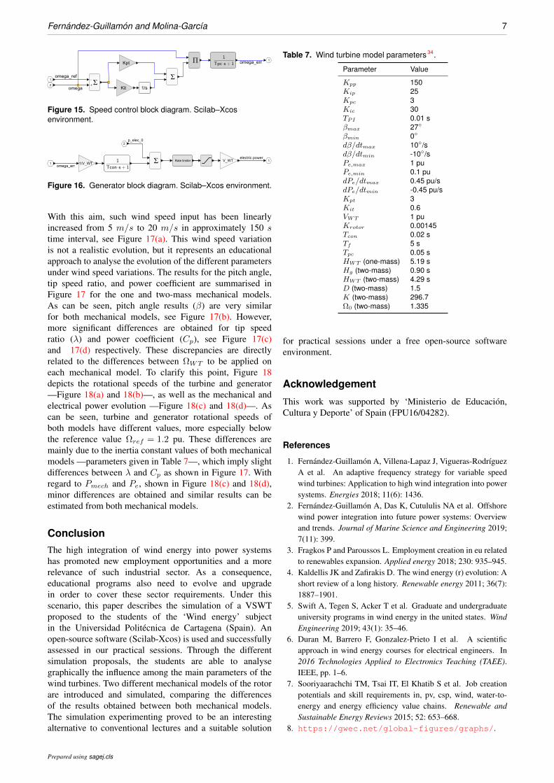
The speed control block estimates the difference betweenthe current rotational speed (Ω) and the reference rotationalspeed value (Ωref ) through a PI controller, as depicted inFigure 15. This error (Ωerr) is sent to the generator andpower converter, determining the electrical power variationdue to such rotational speed error (Ωerr). A subsequentadditional electric power value is then incorporated tothe initial electric power value (p elec 0), as depicted inFigure 16.

Both parameters and values of the implemented modelare summarised in Table 7. These parameters are tunedby using a set of typical wind speed values as an input.



Figure 15. Speed control block diagram. Scilab–Xcosenvironment.

Figure 16. Generator block diagram. Scilab–Xcos environment.

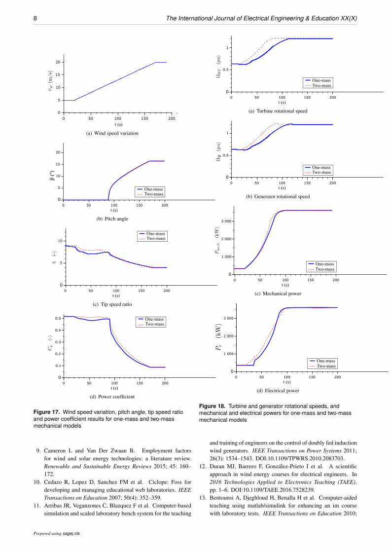
With this aim, such wind speed input has been linearlyincreased from 5 m/s to 20 m/s in approximately 150 stime interval, see Figure 17(a). This wind speed variationis not a realistic evolution, but it represents an educationalapproach to analyse the evolution of the different parametersunder wind speed variations. The results for the pitch angle,tip speed ratio, and power coefficient are summarised inFigure 17 for the one and two-mass mechanical models.As can be seen, pitch angle results (β) are very similarfor both mechanical models, see Figure 17(b). However,more significant differences are obtained for tip speedratio (λ) and power coefficient (Cp), see Figure 17(c)and 17(d) respectively. These discrepancies are directlyrelated to the differences between ΩWT to be applied oneach mechanical model. To clarify this point, Figure 18depicts the rotational speeds of the turbine and generator—Figure 18(a) and 18(b)—, as well as the mechanical andelectrical power evolution —Figure 18(c) and 18(d)—. Ascan be seen, turbine and generator rotational speeds ofboth models have different values, more especially belowthe reference value Ωref = 1.2 pu. These differences aremainly due to the inertia constant values of both mechanicalmodels —parameters given in Table 7—, which imply slightdifferences between λ and Cp as shown in Figure 17. Withregard to Pmech and Pe, shown in Figure 18(c) and 18(d),minor differences are obtained and similar results can beestimated from both mechanical models.

ConclusionThe high integration of wind energy into power systemshas promoted new employment opportunities and a morerelevance of such industrial sector. As a consequence,educational programs also need to evolve and upgradein order to cover these sector requirements. Under thisscenario, this paper describes the simulation of a VSWTproposed to the students of the ‘Wind energy’ subjectin the Universidad Politecnica de Cartagena (Spain). Anopen-source software (Scilab-Xcos) is used and successfullyassessed in our practical sessions. Through the differentsimulation proposals, the students are able to analysegraphically the influence among the main parameters of thewind turbines. Two different mechanical models of the rotorare introduced and simulated, comparing the differencesof the results obtained between both mechanical models.The simulation experimenting proved to be an interestingalternative to conventional lectures and a suitable solution

Table 7. Wind turbine model parameters 34.

Parameter Value

Kpp 150Kip 25Kpc 3Kic 30TPI 0.01 sβmax 27

βmin 0

dβ/dtmax 10/sdβ/dtmin -10/sPe,max 1 puPe,min 0.1 pudPe/dtmax 0.45 pu/sdPe/dtmin -0.45 pu/sKpt 3Kit 0.6VWT 1 puKrotor 0.00145Tcon 0.02 sTf 5 sTpc 0.05 sHWT (one-mass) 5.19 sHg (two-mass) 0.90 sHWT (two-mass) 4.29 sD (two-mass) 1.5K (two-mass) 296.7Ω0 (two-mass) 1.335

for practical sessions under a free open-source softwareenvironment.

Acknowledgement

This work was supported by ‘Ministerio de Educacion,Cultura y Deporte’ of Spain (FPU16/04282).

References

1. Fernandez-Guillamon A, Villena-Lapaz J, Vigueras-RodrıguezA et al. An adaptive frequency strategy for variable speedwind turbines: Application to high wind integration into powersystems. Energies 2018; 11(6): 1436.

2. Fernandez-Guillamon A, Das K, Cutululis NA et al. Offshorewind power integration into future power systems: Overviewand trends. Journal of Marine Science and Engineering 2019;7(11): 399.

3. Fragkos P and Paroussos L. Employment creation in eu relatedto renewables expansion. Applied energy 2018; 230: 935–945.

4. Kaldellis JK and Zafirakis D. The wind energy (r) evolution: Ashort review of a long history. Renewable energy 2011; 36(7):1887–1901.

5. Swift A, Tegen S, Acker T et al. Graduate and undergraduateuniversity programs in wind energy in the united states. WindEngineering 2019; 43(1): 35–46.

6. Duran M, Barrero F, Gonzalez-Prieto I et al. A scientificapproach in wind energy courses for electrical engineers. In2016 Technologies Applied to Electronics Teaching (TAEE).IEEE, pp. 1–6.

7. Sooriyaarachchi TM, Tsai IT, El Khatib S et al. Job creationpotentials and skill requirements in, pv, csp, wind, water-to-energy and energy efficiency value chains. Renewable andSustainable Energy Reviews 2015; 52: 653–668.

8. https://gwec.net/global-figures/graphs/.


https://gwec.net/global-figures/graphs/


(a) Wind speed variation

One-massTwo-mass

(b) Pitch angle

One-massTwo-mass

(c) Tip speed ratio

One-massTwo-mass

(d) Power coefficient

Figure 17. Wind speed variation, pitch angle, tip speed ratioand power coefficient results for one-mass and two-massmechanical models

9. Cameron L and Van Der Zwaan B. Employment factorsfor wind and solar energy technologies: a literature review.Renewable and Sustainable Energy Reviews 2015; 45: 160–172.

10. Cedazo R, Lopez D, Sanchez FM et al. Ciclope: Foss fordeveloping and managing educational web laboratories. IEEETransactions on Education 2007; 50(4): 352–359.

11. Arribas JR, Veganzones C, Blazquez F et al. Computer-basedsimulation and scaled laboratory bench system for the teaching

Two-massOne-mass

(a) Turbine rotational speed

g

One-massTwo-mass

(b) Generator rotational speed

Two-massOne-mass

(c) Mechanical power

Two-massOne-mass

(d) Electrical power

Figure 18. Turbine and generator rotational speeds, andmechanical and electrical powers for one-mass and two-massmechanical models

and training of engineers on the control of doubly fed inductionwind generators. IEEE Transactions on Power Systems 2011;26(3): 1534–1543. DOI:10.1109/TPWRS.2010.2083703.

12. Duran MJ, Barrero F, Gonzalez-Prieto I et al. A scientificapproach in wind energy courses for electrical engineers. In2016 Technologies Applied to Electronics Teaching (TAEE).pp. 1–6. DOI:10.1109/TAEE.2016.7528239.

13. Bentounsi A, Djeghloud H, Benalla H et al. Computer-aidedteaching using matlab/simulink for enhancing an im coursewith laboratory tests. IEEE Transactions on Education 2010;



54(3): 479–491.14. Tortoreli MD, Chatzarakis GE, Voudoukis NF et al.

Teaching fundamentals of photovoltaic array performancewith simulation tools. International Journal of ElectricalEngineering Education 2017; 54(1): 82–94.

15. Moeini A, Kamwa I, Brunelle P et al. Open data IEEEtest systems implemented in SimPowerSystems for educationand research in power grid dynamics and control. In 201550th International Universities Power Engineering Conference(UPEC). pp. 1–6. DOI:10.1109/UPEC.2015.7339813.

16. Das K, Hansen AD and Sørensen PE. Understandingiec standard wind turbine models using simpowersystems.Wind Engineering 2016; 40(3): 212–227. DOI:10.1177/0309524X16642058.

17. Cole S and Belmans R. MatDyn, a new Matlab-based toolboxfor power system dynamic simulation. IEEE Transactionson Power Systems 2011; 26(3): 1129–1136. DOI:10.1109/TPWRS.2010.2071888.

18. Milano F and Vanfretti L. State of the art and future of OSS forpower systems. In 2009 IEEE Power Energy Society GeneralMeeting. pp. 1–7. DOI:10.1109/PES.2009.5275920.

19. Hsu HmJ. The emergence of Free and Open–Source Softwareon Campuses in Taiwan. In Proceedings of the 2012 IEEEGlobal Humanitarian Technology Conference. Washington,DC, USA: IEEE Computer Society. ISBN 978-0-7695-4849-4,pp. 403–407. DOI:10.1109/GHTC.2012.58.

20. Nehra V and Tyagi A. Free open source software in electronicsengineering education: a survey. International Journal ofModern Education and Computer Science 2014; 6(5): 15–25.

21. Seixas M, Melıcio R and Mendes VMF. Simulation by discretemass modeling of offshore wind turbine system with dc link.International Journal of Marine Energy 2016; 14: 80–100.

22. Elias M. Impact of the bologna process on spanish students’expectations. International Journal of Iberian Studies 2010;23(1): 53–62.

23. Harmsen R. Future Scenarios for the European HigherEducation Area: Exploring the Possibilities of ’ExperimentalistGovernance’. Cham: Springer International Publishing. ISBN978-3-319-20877-0, 2015. pp. 785–803. DOI:10.1007/978-3-319-20877-0 48.

24. Njiri JG and Soeffker D. State-of-the-art in wind turbinecontrol: Trends and challenges. Renewable and SustainableEnergy Reviews 2016; 60: 377–393.

25. Sharma N and Gobbert MK. A comparative evaluation ofmatlab, octave, freemat, and scilab for research and teaching.UMBC Faculty Collection 2010; .

26. Vijayalakshmi S, Anuradha C, Ganapathy V et al. Directdriven wind energy conversion system connected to loadusing variable frequency transformer. The InternationalJournal of Electrical Engineering & Education 2019; :0020720919829011.

27. Kouroussis G, Fekih LB, Conti C et al. Easymod: Amatlab/scilab toolbox for teaching modal analysis. In 19thInternational Congress on Sound and Vibration (ICSV19),Vilnius, Lithuania.

28. Glavelis T, Ploskas N and Samaras N. A computationalevaluation of some free mathematical software for scientificcomputing. Journal of Computational Science 2010; 1(3):150–158.

29. Rubtsova A and Korolev V. Scilab. creating graphicalapplications. In Abstracts of XXIII international scientific and

practical conference of young scientists and student, volume 2.p. 292.

30. Arianto S, Yunaningsih RY, Astuti ET et al. Developmentof single cell lithium ion battery model using scilab/xcos. InAIP Conference Proceedings, volume 1711. AIP Publishing, p.060007.

31. Tona P. Teaching process control with scilab and scicos. In2006 American Control Conference. pp. 6 pp.–.

32. Qin Y, Korkali M, Top P et al. A JModelica.org library forpower grid dynamic simulation with Wind Turbine Control. In2019 IEEE Power Energy Society General Meeting (PESGM).pp. 1–5.

33. Kanoj B, Sanu MA and Raju AB. Steady state analysisof autonomous wind energy conversion system for irrigationpurpose employing induction machines using python — a freeand open source software. In 2013 IEEE Global HumanitarianTechnology Conference: South Asia Satellite (GHTC-SAS). pp.292–297.

34. Miller NW, Sanchez-Gasca JJ, Price WW et al. Dynamicmodeling of ge 1.5 and 3.6 mw wind turbine-generators forstability simulations. In Power Engineering Society GeneralMeeting, 2003, IEEE, volume 3. IEEE, pp. 1977–1983.

35. Ullah NR, Thiringer T and Karlsson D. Temporary primaryfrequency control support by variable speed wind turbines– potential and applications. IEEE Transactions on PowerSystems 2008; 23(2): 601–612.

36. Villena-Ruiz R, Jimenez-Buendıa F, Honrubia-Escribano Aet al. Compliance of a generic Type 3 WT model with theSpanish Grid Code. Energies 2019; 12(9). DOI:10.3390/en12091631.

37. Molina-Garcıa A, Fernandez-Guillamon A, Gomez-Lazaro Eet al. Vertical wind profile characterization and identification ofpatterns based on a Shape Clustering Algorithm. IEEE Access2019; 7: 30890–30904. DOI:10.1109/ACCESS.2019.2902242.

38. Ragheb M and Ragheb AM. Wind turbines theory-the betzequation and optimal rotor tip speed ratio. In Fundamental andadvanced topics in wind power. IntechOpen, 2011.

39. Ata R and Kocyigit Y. An adaptive neuro-fuzzy inferencesystem approach for prediction of tip speed ratio in windturbines. Expert Systems with Applications 2010; 37(7): 5454–5460.

40. Martınez-Lucas G, Sarasua J and Sanchez-Fernandez J.Frequency regulation of a hybrid wind–hydro power plant inan isolated power system. Energies 2018; 11(1): 239.


Documents

Simulation of Variable Speed Wind Engineering & Education