SIMULATION AND PERFORMANCE ANALYSIS OF A

SHIPBOARD GAS TURBINE EMERGENCY GENERATOR SET

Phil Id J. Grossweiler

SIMULATION AND PERFORMANCE ANALYSIS OF A

SHIPBOARD GAS TURBINE EMERGENCY GENERATOR SET

by

PHILIP J.^GROSSWEILER III

B.S. , United States Coast Guard Academy

(1966)

SUBMITTED IN PARTIAL FULFILLMENT OF THE

REQUIREMENTS FOR THE DEGREES OF

MASTER OF SCIENCE IN MECHANICAL ENGINEERING

and

MASTER OF SCIENCE IN NAVAL ARCHITECTURE AND MARINE ENGINEERING

at the

MASSACHUSETTS INSTITUTE OF TECHNOLOGY

May, 1972

-2-

SIMULATION AND PERFORMANCE ANALYSIS OF A

SHIPBOARD GAS TURBINE EMERGENCY GENERATOR SET

by PHILIP J. GROSSWEILER III

Submitted to the Departments of Ocean Engineering and MechanicalEngineering on May 12, 1972, in partial fulfillment of the requirementsfor the degrees of Master of Science in Naval Architecture and MarineEngineering and Master of Science in Mechanical Engineering.

ABSTRACT

The objective of this study is to model and simulate using an Analogcomputer the performance of a relatively complex engineering system. Theresults of the simulation are validated by a comparison of the simulationwith the measured performance of the prototype system.

The prototype system consists of a single shaft gas turbine enginedriving a three-phase alternator. The alternator load is a variable speedthree phase wound rotor induction motor which drives a ship bow thrusterpropeller. In order to provide sufficient data to validate the simulation,the alternator speed, current and terminal voltage, KW load, and inductionmotor speed are recorded continuously as the motor is switched through five

speeds. The recorded transients in these variables are then used to validatethe model and simulation.

The system is segregated into five sections and analytical models are

determined for each component. The gas turbine is modeled using a transferfunction derived from the engine performance curves. The speed governingsystem is modeled using transfer functions for the governor components £3

supplied by Woodward Governor Company. The alternator model is a result of

the work of Professor Paynter and is taken from notes from his subject"Dynamics and Control of Rotating Machine Systems." The induction motormodel is derived from a simplified equivalent circuit. The propeller is

modeled as a torque proportional to the square of the speed. The simula-tion is simplified considerably by using a single-phase model to representthe electrical machinery.

The correlation between the simulation and the prototype performanceis excellent. The models used are relatively simple and yet can provideclose estimates of the system performance and can demonstrate how perform-ance varies as the system parameters are changed.

Thesis Supervisor: Henry M. PaynterTitle: Professor of Mechanical Engineering

Thesis Reader: Warren C. DietzTitle: Associate Professor of Marine Engineering

-3-

ACKNOWLEDGEMENTS

I would like to first thank my wife Diana for the patience she has

shown during the last two years of school work, and especially during the

last term.

During this study valuable assistance has been received from many

individuals and in various ways. The most important has been the advice

and guidance received from Professor Paynter, both during this study and

in previous course work.

I am particularly grateful to Mr. Henry Egan of the Boston Naval

Shipyard for providing me with the equipment required for monitoring the

performance of the prototype system.

The cooperation of the United States Coast Guard First District

Naval Engineering Branch and the engineers of the USCGC BOUTWELL and the

USCGC CHASE was indispensible in making the required recordings of the

system operation. In particular, the willingness of Chief Electrician

Duke to allow an outsider to connect wires and recorders to various sec-

tions of the BOUTWELL 'S electrical equipment was most encouraging. With-

out his willing help, it would have been most difficult to obtain system

data.

Also, I would like to thank Richard S. Sidell for his assistance

over the past four terms with the EAI-6 80 Analog computer.

Finally, I would like to thank Mrs. Jack "Sam" Price for her excel-

lent and efficient work in typing this paper.

-4-

Title Page 1

Abstrac- 2

Acknowlecgr.er.rs "^

Table cf lor. tar.rs ^

5

List of Svricls ^

1. Introducticr. ^

2. Description of Prototype System ^^

3. Instrunentatior. ar.d P.eccrdir.g Procedures 23

4. Systen Models

4.1 Gas Turbine 28

U.2 Governor Section ^^

4.3 Alternator 32

4.4 Induction Motor **"^

4.5 Propeller ^2

4.5 Bearing Resistances ^^

5. Siinulation

5 . 1 Parar.eter Zstirr^ates ^^

5.2 Analog Setuc 50

5.3 Scaling .analog Siimilation

7. Conclusions and Recommendations

58

6 . Results^"^

B^^

pqReferences

-5-

LIST OF ILLUSTRATIONS AND TABLES

Illustrations Page

1. Prototype System Bond Graph .16

2. Cutaway View Saturn Gas Turbine Engine ' 17

3. Reduction Gear Drive Arrangement 18

4. Saturn Engine Performance Curves 19

5. Governing System Schematic 20

6. Schottel Bow Thruster Arrangement 21

7. Propeller with Nozzle 22

8. Instrumentation Bond Graph 27

9. Analog Computing Diagram 57

10. Prototype Measurements and Simulation Results 69

11. Induction Motor Performance Curves with Simulation Results 83

12. Engine and Governing System Block Diagram 31

13. Engine and Governing System Block Diagram 58

Tables

1. Amplifier Assignment Sheet 6M-

2. Potentiometer Assignment Sheet 66

3. Correlation of Alternator Speed 78

M-. Correlation of Induction Motor Performance 79

5. Comparison of Estimated Parameters with Values Used in Simulation 80

-5-

LIST OF SYMBOLS

ALT Alternator

a Governor constant

Oi Fuel control actuator buffer spring stiffness

02 Fuel control actuator constant

03 Fuel control actuator needle valve setting

3 Propeller water velocity angle

C^ Propeller torque coefficient

CT Current transformer-

D Propeller diameter

E, e Voltage

E^ Governor error signal

E3 Output of governor amplifier section

FCA Fuel control actuator

FCV Fuel control valve

GCB Governor control box

Y Governor stabilizing section damping ratio

I_ Alternator line current

If Alternator field current

Igq Inertia of all components driven by gas turbine

Iju Inertia of motor

Ip Inertia of propeller

IM Induction motor

K Gain of governor amplifier section

Kf Fuel control actuator constant

-7-

K^ Engine torque constant

Lg Alternator Inductance

Lju Motor inductance

N Speed in RPM

AN Deviation of alternator speed from base speed

Npgf Base speed of alternator and motor

m Air flow rate

m^ Fuel flow into engine manifold

Wf' Fuel flow into fuel control valve

Wf Fuel flow into engine manifold

P. Ambient pressure

?H Engine exhaust pressure

PT Potential transformer

R2 Bearing resistance of engine and alternator

R3 Bearing resistance of induction motor and propeller

Rg^ Motor rotor resistance

Rg' Added rotor resistance

4'f Dynamic operator representing fuel control valve action

p Water density

s Laplacian operator

.Angle of fuel control actuator shaft

max -

Q . Maximum travel of fuel control actuator shaftmmT Engine mechanical time constant

T Torque

T Normalized torque (x/Tpg-f)

-8-

T- Alternator torque

Tg Engine torque

T Motor torque

Tn Engine inlet temperature

Tn Engine exhaust temperature

TFn Bond Graph symbol for engine speed reducer

TF2 Bond Graph symbol for motor speed reducer

Vq Axial water velocity through propeller

V Tangential velocity of propeller blade at maximum diameter

0) Speed in radians per second

0)- Motor synchronous speed

X Electrical reactance

X _ Equivalent reactance of motoreq

Xgg Synchronous reactance of alternator

-9-

1. INTRODUCTION

Simulation has become one of the most important tools available

to engineers in the study and design of complex physical systems. The

ability to predict a system's response to various inputs is useful in

many ways. Actions which can have disastrous effects on a system can

be avoided if accurate predictions of the system response are avail-

able. Simulation can also aid in the realization of high levels of

system performance by aiding in control system design. Studies of the

effects of varying system parameters can be performed with a simulation

so that an optimum or near optimum prototype can be built without a

costly trial and error process.

The first stage in simulating a complex physical system is to i-

dentify the individual components. An attempt is then made to formulate

a model for each component of the system so that the interconnected m.od-

els will predict the performance of the system within a specified level

of accuracy. Simulation is in effect a four-stage process. In the

first stage the system is reduced to individual components and "black

boxes" are used to represent these components. In the second stage,

the components are Interconnected so as to reflect the structure of the

prototype system. The third stage usually requires the use of a com-

puting machine to determine the time history of the variables as the

components interact with each other.

This simulation procedure can be carried out almost completely us-

ing the concept of Bond Graphs (1), (2). Although bond graph techniques

can be used to develop a set of state equationrs representing the entire

-10-

system, for this simulation bond graphs will be used primarily to dis-

play the structure of the system. The Bond Graph method enables one

to visualize a system as a set of multi-port devices connected by power

bonds. As a result of this partitioning of the system the energetic

interactions across the boundaries are clearly shown. For the case of

the prototype system under study the basic bond graph representing the

main power flow is as follows

:

Gas ^ AT^ ^ ^w Induction . d^^t^^it^^.

N»,Altemator X .. \ PropellerTurbine Motor

Each component is a multiport which interacts with the rest of the

system through the power bonds as shown. Associated with each bond

are the power variables (T, u or e , i) which determine the power flow

between the multiports.

The models required for the multiports shown above can be deter-

mined in various ways. However, regardless of how the models are de-

termined, they should satisfy the following conditions:

1) The time history o f the power variables at each port when connected

to the system should in the simulation match that of the corresponding

prototype parts over the ranges of variables and frequencies being con-

sidered.

2) Each mod-^1 should be as simple as possible consistent with the ac-

curacy required for the simulation. Unnecessary complexity will in-

crease the cost of simulation and will tend to obscure the more impor-

tant points. More important however is the need to adapt the simulation

to available computer facilities. Frequently, as in this case, the

-11-

simulation must be simplified because of limitations of the available

computing equipment.

There is no unique method of modeling system components. However,

any method can be classified as being either analytical or empirical.

Analytic methods rely on use of the basic engineering disciplines and

in effect derive a model from first principles. Although in principle

analytic methods can be used to model any device, these methods become

extremely difficult to use for very complex components. Empirical

methods are in effect a transfer function approach to modeling. Given

a component and information about its performance und-r specified con-

ditions, it is usually possible to infer a relationship between the in- .

put and output variables. For multiple input-multiple output systems

this technique may become difficult to use. Also, this method gives no

information about the internal operation of the component. However, for

studies where only interactions with the rest of a system are considered

this method is perfectly adequate.

In this study the models are determined using both methods. The

alternator model is based on an analytic derivation whereas the model

for the gas turbine is derived from performance curves. The models used

for this simulation are discussed in detail in the following sections.

The question most frequently asked during this study was "Why simu-

late a system which has already been built?" The final stage in any sim-

ulation is validation of the results. Although in most cases the simu-

lation must be validated without prior knowledge of the prototype, models

which have been proven with one prototype can be used with great confi-

dence for a large family of similar systems. In effect, the best

-12-

documentation of a system model is by comparison with observed perform-

ance of a prototype. A large part of this study deals with collecting

sufficient operating data from the prototype system in order to validate

the models used.

The prototype was selected because it provided the opportunity to

model an interconnected system which included mechanical and electrical

machinery with feed-back control on the energy source. Equally im-

portant was the ability to instrument the system in order to record

sufficient operating data to validate the model. The prototype selected

was the gas turbine emergency generator set and bow propulsion system on

the USCGC BOUTWELL which is located in Boston, Massachusetts. The pur-

pose of this study is to simulate the effects of the transients in the

system caused when the bow thruster motor is started.

-13-

2. DESCRIPTION OF PROTOTYPE SYSTEM

The p rototype system is shovm in detail in the bond graph shown

in Figure 1. The prototype system is defined from an arbitrary choice

of equipment installed on the ship. The emergency generator can be

used to supply electrical power to any load on the ship as shown in the

sketch below. The bow thruster is a trainable propeller which is used

to provide a directional thrust at the bow when docking the ship. The

unit is retracted into the ship when not in use. The electrical system

can be interconnected so that the bow thruster is the only load on the

emergency generator. The prime mover is a single shaft Solar Saturn

Gas Turbine. For standard atmospheric conditions the engine is rated

at 1200 HP at 22,300 RPM. The output is reduced through a two stage

planetary gear box to 1200 RPM. An engine cutaway view, arrangement of

reducing gear and engine performance curves are given in Figures 2, 3,

and 4.

The engine speed is controlled by a Woodward EG series governor.

The governor system is shown in the schematic on page 20. The two main

components are the EGA Control Box and the EGB-2C Actuator. The gover-

nor can control the engine in either isochronous or droop mode. The

actuator can also control the speed using the conventional mechanical

flyweight assembly. For this study the system will be controlled

electrically and in the isochronous mode. The operation can best be

described by the transfer functions for the components. The transfer

functions supplied by Woodward Governor Company are of the following

form:

-14-

r - -1.5 A N ^ 0.00405 S f , • -, \£ _ _ j..^ — ^ _. e_ (error signal)-^ NrE s/10 + 1 Tj^^^

-1 = ./ ^^ ^ '^-' (amplifier section)E]_ s^ + YS + o

, 0_ __33.3 a2(s

| ^^) ^^^^_^^ Actuator)E3 sis + a-j_)

These signals are shown in the governor schematic. Figure 5.

The error signal is a combination of a voltage proportional to the

error in speed and a voltage output from the load sensing network which

provides lead compensation. The governor response can vary over a wide

range depending on the values of the following parameters:

(1) Feedforward gain of the load sensing network (O. 00405)

(2) Gain of the amplifier section (K)

(3) Damping ratio of the stabilizer section (y)

(4) Buffer spring stiffness (a-,)

(5) Needle valve setting (03)

The alternator is a General Electric machine with the following

characteristics

:

Rated KVA 525 Speed 1200 RPM

Rated KW 500 Winding 3 Phase

Rated P.F. 0.8 Connection Y

Rated Volts 450 Frequency 60 Hz

Rated Amps 801 Poles 6

Voltage regulation is provided by a static excitation system.

The alternator is connected to the ship's electrical system in the

following way.

-15-

Emergency

Generator

EmergencySwitchboard

#2

Switchboard

#1

Switchboard

Eor this study the system is set up so that the emergency generator is

supplying only the Bow Thruster load.

The Bow Thruster Unit is shown in Figures 6 and 7. It is manufactured

by Schottel of America, Inc. The driving motor is a General Electric three-

phase wound rotor induction motor with the following ratings:

Rated Volts 440 Rated Amps 440

Speed 1180 RPM Torque 1550 Ib-ft

HP 350 Frequency 50 Hz

The motor performance curves are shown in Fig'ore 11. The motor is started

with full line voltage applied and additional resistance in the rotor cir-

cuit. Five propeller speeds are provided by shunting the external re-

sistors in four steps. The shunting of these resistors is controlled by

time delay relays. The motor is connected to the propeller through a

vertical shaft and bevel gears.

The propeller is enclosed in a nozzle as shown on page 22. The

diameter is four feet, pitch 28.819 inches and the reduction ratio from

the motor speed 2.079:1.

-16-

W

p=:oQ*--

»

* Or— P^:

Hto CI•H >-:

1^ 03

Wa,IHE^O&4O«

m«

OJrH

A-7

^^ r >—O— O

1E-i

/IOJ

\

K>

eWpq X

t-t

"7?. V L-l

-O

>o

/I

<M

K

\/ >^

pqoo

ofi4

-17-

Figtore 2.

in

nto

I

QA

(J

CMCuVa

u3

aCbi

3?i

x>

oa>.

H

0)

3u

3b£

Drawing Courtesy of SOLAR Inc.

18-

Flgure 3,

liINd

a.

SUN

KING GEAR(STATIONAKY)

ni.\C CEAJ^

2NXI-t>TAGEOUTPUT

PL.\NtT Gt.\KC.\HKItR

Itt-STAGE

PLANET GEAR CARRIEROMITTED FOR CLARITV

Drawing Courtesy of SCLAR I?IC,

-19-

in

nI

Q

• r\ I'll' Al rh HKlUMANCK SA 1 I UN(.A.s aullINK KM.l.SK .,01) KW (.fNHIAIOH

Figure •+.

~0. 27

/mo INl.KI AND KXHAt'Sr DL'CT PHKSSIKK " 26l.OSSIS AT 1(10 l-mc'KNl KATKI) KNCINK SI'KKl) fa

SKA 1 KVH. <

• 1MI- II UHISK HKNKHATdH SKT IS HATKI)AT r.OO KW .

II PI PK, MAXIM! M COSTINl ( IL'S

(iPf HATION Ul TH (nHU.OAl) CAPAnil.lTVOy lU PKRCKN r KOn 2 HOI US IN ANY 24 llOtltI'HtlOl),

• ': 1

1

I'

1

1

^-1-14 +-

Mi:MMM <

i!!p«"

ipi.f:•

*- i—i--

t

t

^i

. .1

»

1

1 1

300 400 500 600 700 800 900

EXHAUST GAS TEMP 'F

I \(,1M All! MASS h LOW (^\ ) TIIOI SANDS I'MIt

.1 "ill I'J th

20 30 40 50 60 70 90 90

ENCrNE INLET AIR TEMPERATURE (T,!'' F

100 110

Output Power (KW) vs Engine Inlet Air Ter.:.'erature

Drawing Courtesy of SOLAR INC.

-20-

Figiire 5»

Governing Systen Schematic

WSSSSSED

L_-.HYDRiUlIC

tCTUtlOR^—^ ENGINE hU^ GENERATOR PPi 1

left : Nornidl Posilion \Single unit isochionous conliol ot parallel wilh other EG governors ^

Right : Droop Posilion

DROOP SWITCH —-___ Parallel with infinite bus or dissimilar governors

Circuit Breaker

^iUXIllARY C0NI4CI

L_

-o o- PiRiUElING LINE

to Other Units

^

PlRtllElING ,

I NETWORK I

I I

£o . AMPIIEIER SECTION— —

I

(Gain)I

I

(Adjustable) |"*~

STABILIZER SECTION

H (Stability) |—

I

(Adjustable) .

-UI

I JLOAD SECTION r-^

—I (load Gam)'

I

(Adjustable)

DROOP SECTION

(Adjustable)

LOAD

I

SPEED SECTION [^ '

I I

I I

ISPEED REFERENCE i^

1 SECTION r*~

I I

CONTROL SOX

Drawing Courtesy ofwooDV/ARD gover:.'OR cc: fa:.t

(Bulletin ?7706B)

-21-

\D

W)

(t:^

H<:un

+> «c Cd

^<U

bO «rH

C O rocC 1

(h

EH

ITN

^ COH

^1 o ^0) CD+J CJ ,0

piW

§^1 <H ^:

X OH bO

>. C^ m •Ho 0) >pq 4J CO

H ^o op o+Jc W)x: co •HCO

-22-

Figure 7.

Bow Propeller With Nozzle

H2

i5*a*b

SCHOTTEL- NEDERLAND N.V. D E N H A A G — WA R M O N D

-23-

3. INSTRUMENTATION AND RECORDING

Verification of the system model and simulation by comparison with

the prototype performance requires records of the system variables during

operation. The optimum choice for recorded variables are the state varia-

bles of the system model. In this case the choice of observed variables

was limited to measurements which could be made without major modifica-

tions to the prototype and which did not require excessive time or cost.

As a result, most of the observed variables were chosen because the proto-

type was instrumented to monitor these variables. However, these con-

straints did not prevent obtaining a set of observables sufficient for

model verification.

The complete instrumentation setup is shown in the bond graph in

Figure 8. The main power flow through the system is shown with heavy

lines. The boxed items show all sensors, signal conditioners and record-

ers which were added to the prototype instrumentation. Each box is la-

beled with the variable recorded. All bonds to the boxes are active, i.

e., zero power flow into the recorders is assumed. Details of each meas-

urement is given below.

Results were recorded on a Clevite Mark 220 Brush Recorder. This

instrument is very versatile and provided satisfactory records of all

variables measured. Input signals ranged from five millivolts to fifty

volts and in frequency from D.C. to 50 Hz. For full scale deflections

the frequency response is flat up to 40 Hz. The frequency response can

be increased to 100 Hz if the meter movement is limited to twenty percent

of the full scale.

ALTERNATOR LOAD The EGA Control Box Load Section senses the

-24-

altemator terminal voltage and current through potential and current

transformers. A correction Is made for power factor so that the output

of the load section Is a signal with a D.C. level proportional to the KW

load. At full load the D.C. level is approximately nine volts. However,

this value will vary depending on the values of the resistors used with

the current transformers, the levels of voltages and currents delivered

by the instrument transformers and the gain of the load sensing section.

The load signal contains harmonics of the line frequency in addi-

tion to the D.C. level. Since the amplitude of these harmonics was ap-

proximately twenty percent of the D.C. level an RC low pass filter with a

time constant of 0.06 8 seconds was used to filter the harmonics.

FIELD CURRENT The full load field current is approximately seventy

amps at seventy volts. A shunt resistor was inserted in the field circuit

at the brush rigging. The shunt resistor voltage drop is fifty millivolts

at seventy-five amps.

ALTERNATOR SPEED The installed tachometers and frequency meter are

used primarily for steady state observations. Large errors in measuring

transients can be expected when the time Interval of the transient ap-

proaches the time constants of the meter movements . As a result , the

meters cannot be used to accurately record transients resulting from step

changes in load.

The speed measurement was made using a Clevite Corporation Frequency

Converter. The converter is calibrated to give a D.C. signal proportional

to the change in frequency. A deviation of ± 5 Hz from the base frequency

gives a ± 2.5 volt output. The rise time of the output signal is 0.060

-25-

seconds. This response together with the response of the recorder gives

an accurate measure of the speed transient.

The signal input to the converter is at 110 volts in the range 55-55

Hz. The prototype system was set up with the alternator supplying the

emergency switchboard so that the bow thruster was the only load. In

order to provide a 110-volt signal at the alternator frequency for input

to the converter, the 110-volt lighting circuit at the emergency generator

was supplied from the emergency board. This total lighting load is less

than five KW so that the effect on the alternator is negligible. The al-

ternator load is assumed to be from the bow thruster motor only.

TERMINAL VOLTAGE The terminal voltage was recorded using a Clevite

Corporation Volts Converter. The recorder delivers a D.C. voltage propor-

tional to the peak A.C. voltage. The converter was driven by the 220 volt

output of the load sensing network potential transformer.

ARMATURE CURRENT The armature current was recorded from the voltage

across the input resistors to the load sensing network. The current to

these resistors is supplied by the current transformers connected across

the main line. Since this signal was at the 60 Hz line frequency the

maximum amplitude of the recorded signal was limited to approximately

twenty percent of the chart deflection in order to have satisfactory fre-

quency response

.

BOW THRUSTER SPEED The induction motor drives an A.C. tachometer

generator. The tachometer output was recorded directly on the Brush Re-

corder. Speed can be determined either from the instantaneous frequency

or voltage amplitude. For 1200 motor RPM the tachometer frequency is

-26-

40 Hz. The tachometer signal was recorded full scale on the chart since

the recorder frequency response is flat to 40 Hz.

-27-

Figure 8.

iiistrui-:e::tatioii boiid graph

4J O

<v:i

s It- enQc^.o q'f>o w !^;

r-:i p:^ O1—4 P^ O

m̂o

^ ; CO

'id

@ 0)

Q cu^ COOo infj op:; +->

o

O

EHa,

Ken t'-:

H L-i

.-? Pio M> r'

oo

«

^

o—.@1 P,1 <^-'

1K (

1 o^ gB p^K—

(

CQ

-P

/\

oo

o

rt

aM

K!

>O

28-

U.l GAS TURBINE MODEL The derivation and final structure of the

gas turbine model depends on the type of study involved. In one type of

study, knowledge of internal behavior in response to changes in environ-

ment and load is required. In other studies, only knowledge of the time

history of the i nput /output variables is required. Obviously for the

latter case the model can be simpler and will most likely be in the form

of a transfer function.

In reference (10) a model is derived from basic principles for a

single shaft gas turbine where it is shown that the gas turbine can be

represented by a multiple input-multiple output transfer function of the

following form.

Pi

Tl

N

"^fb

-^

Gas

Turbine

Engine

^>- "^•

The matrix representing the input and output vectors is a relatively com-

plicated non-linear function of the internal variables and engine charac-

teristics. For this case the model can be simplified considerably and

will be used in a linearized form.

The most valuable information provided by this formulation is an indi-

cation of the functional relationships which exist between the input and

output variables. Since the mass flow rate (m) is not being considered,

only the functional relationship for torque is needed. From the transfer

function it is seen that

T = <I>(Pi, T^, P4, N, mf^)

-29-

For this study, the ambient conditions P-, and T-, can be assumed constant.

For a constant mass flow rate, fixed geometry and constant ambient condi-

tions the exit pressure P^ is also relatively constant. Since the mass

flow rate is primarily a function of the speed, which is relatively con-

stant, "the only input variable which changes significantly is the fuel flow

rate liifv. As a result the functional relationship can be reduced to:

T = $'(mf:^)

This functional relationship can also be derived by considering a

control surface around the engine.

Air Flow ) —^ Air Flow

Engine

Fuel Flow ^ —^ Shaft Power

For this case where the engine can be considered small with respect to its

ability to store energy as a result of either mass or thermal capacity,

the changes in stored energy can be neglected. From observations on the

prototype, it is known that the temperature of the exhaust gas is relative-

ly constant throughout the operating range. With a constant air flow rate

and exit velocity the enthalpy of the entering and leaving gases is rela-

tively constant. As a result, the primary energy quantities entering and

leaving the control surface are in the fuel flow and shaft work. With all

of the assumptions above it is seen that output power is proportional to

input fuel. Since speed is relatively constant it follows that

T = $'(mf]3) = KtiTif^

This relationship is verified by the engine performance curves given

in Figure 4. Since the output KW is proportional to torque at constant

-30-

speed, the torque is proportional to fuel flow rate for constant T-, .

In a simulation, it is necessary to consider the effects of the

engine dead time or transport delay. This delay is defined as the time

interval between a change in fuel flow rate and the change in torque out-

put. From the control surface above, it is seen that this delay depends

on the ability of the engine to store energy and the speed at which changes

in internal temperature resulting from fuel rate changes can propogate

through the engine. As stated above, the storage effects can be neglected.

An estimate of the delay due to propagation time can be made by consider-

ing the transit time for sound waves through the engine. This is the speed

at which the temperature changes resulting from fuel rate changes propogate,

For the Saturn engine, the transit or dead time is on the order of 0.005

seconds. The torque relationship is then modified as follows:

^ _ ^, -Ts- ~ ^ "'fbT - K^e nif^ = 1 + Ts

The delay is approximated by a first order lag for the purposes of analog

computation.

All that is necessary to develop the turbine model is to determine the

torque coefficient from the performance curve. This coefficient is a func-

tion of ambient temperature with K^ decreasing with increasing ambient tem-

perature. It will be shown below that when the system block diagram is

non-dimensionalized for the analog computation, the torque constant can be

lumped with the overall loop gain.

4.2 GOVERNOR SECTION The governor schematic is shown in Figure 5.

The engine block diagram can be formulated directly from the schematic us-

ing the governor transfer functions supplied by Woodward Governor Company.

31-

load

.0

0.0045 s

(s/10+1) T^gf

_1_

Is o K2 (s + a) 33.3a2(s+a3)s(s + a-]_)

Figiore 12.

From the diagram it is seen that if the delay is neglected

^e= ^T-^fb = K/Yf = K^'Kf e

where it is assumed that the fuel flow is proportional to the angle of the

fuel control valve. Although in most cases this relationship is approxi-

mately linear, slight non-linearities will not affect the overall system

performance. Although the fuel control valve is actually a dynamic opera-

tor, in this case the valve will be considered to be a static operator.

For low frequency changes in fuel angle this is a good approximation.

With Kj = K^'Kf ; x = K^0 Taking t = T^^p when = (Q^ax ' Qmin)>

where (©max ~ ®min^ ^^ "*^^^ maximum travel of the fuel control actuator,

the torque constant K^ is

K^ =T^REF

^0Tn;.v -max ^mm

."»I

-32-

In reference (10) it is shown that if the loop gain K2 is not exces- .

sive the gain and phase margins at the crossover point of the open loop

transfer function (approximately 5 rad/sec) will be adequate and the action

of the stabilizer section of the control box [ •) can be neglected,s + Ys + <^

This simplification neglects the response of the governor system to fre-

quencies above approximately 50 rad/sec. With the stabilizer section ne-

glected and using the nominal values for the governor settings, the system

block diagram is as shown in the section on Analog Scaling page 58.

4.3 ALTERNATOR MODEL The study of alternators typically involves

deriving an equivalent circuit and phasor diagram of the electrical varia-

bles. However, the phasor diagram does not explicitly show the mechanical-

electrical energy conversion process which is a major part of the prototype

system's power interactions. The model used for the simulation must in-

clude the torque -current and speed-voltage relationships involved in the

energy conversion process. Such a model can be derived from a study of

the energy interactions of idealized magnetic circuits. The model proposed

by Paynter, reference (10),was formulated this way and as a result shows

the structure of alternator as a gyrator-type converter as well as the

behavior of the electrical variables.

The major assumptions required to simplify the analytical derivation

of the alternator model are that the magnetic circuits are not saturated

and that all fluxes are linear functions of the currents. The lineariza-

tion reduces the problem to a study of linear-coupled circuits and allows

superposition of the magnetic fields. It is also assumed that the air

gap is uniform. However, in a study of terminal voltage, current, torque.

-33-

and speed relations under load conditions, salient pole effects are rel-

atively minor and can be neglected. One of the main effects of saliency

is to produce a reluctance torque, and, except at no load, this torque

is negligible compared to the total torque. The resulting model can then

be used for machines which are operated under quasi -linear conditions and

can be used for modeling the prototype alternator.

The basic variables and relations required for the derivation are as

follows

:

X = flux linkage = N(j)

N = effective turns ratio of winding

({) = equivalent flux linking all terms = PF

P E permeance

F = magnetomotive force = Ni

F i

Wjjj'« E co-energy in magnetic field =J

(()(F)df = Jx(i)dj[o

The inherent behavior of polyphase machines is the same regardless of

the number of phases. As a result the torque is determined by the current

flowing in each phase and the number of phases. In the balanced Dolyphase

machine each phase torque is a pulsating torque at twice the line fre-

quency with a D.C. level which is exactly the total torque divided by the

number of phases. When all phase torques are summed the pulsating torques

cancel so that the total torque is constant in the steady state.

A reasonably accurate model of the alternator (and motor) can be made

using only a single phase if the torque pulses can be neglected. Alternators

with large inertias behave dynamically as low pass filters as seen from the

simplified bond graph and system equations for a rotating mass.

sT ^

Where - = — Where I = ^^T Is + R g

For the prototype system I is on the order of 2000 Ib-ft and 2co

the frequency of the torque pulsations is 754 radians per second. Since

R is relatively small;

where co is the fluctuation in speed

<< 12000 ^ ^^^^ caused by the pulsating torque.32

The inertia of the induction motor and load is the same order of mag-

nitude so that a single phase model can be used for both with torque pulsa-

tions being filtered by the relatively large inertias.

The alternator model used below is taken from, one phase of a two-

phase alternator model. Although the model is derived for a two-phase

machine, one phase can be used to represent one phase of a three-phase

machine since the torque pulsations are both double -frequency pulsations

and are filtered by the inertias. All that is required to use this model

for a three-phase machine is to properly scale the D.C. level of the

torque

.

The two-phase representation shown below is very similar to the Park's

dqo transformation used in studying three-phase machines. In this case the

variables are referred to the two-phase stator whereas in the dqo trans-

formation the variables are viewed with respect to the rotor.

-35-

> a

Total flux linking coil a

>^a.= NaPCNaig + NfifC] (1)

Total flux linking coil b

Xb = NaPCNaib + Nfi^S] • (2)

Total flux linking coil f

\f = NfPCNaiaC + NaibS + Nfif] (3)

Where Ng = Nj^ Me NaNfP

C = cos N E Na^

S = sin

and the permeance is independent of in accordance with the assumption

of a smooth air gap.

Now W^»'* = /C^adi^ + Xi^di^ + A^dif]

V = /[^PNiadia + CMifdia + PNi^dii^ + SMifdi^ + CMigdif + SMifadif

+PNf2ifdif] = i^PNCia^ + ib^l +''2PNf:2if2 + MifCCi^ + Si^] (4)

-36-

For any electro-mechanical converter

3Wl= T30

so that T = Mi^ [-Si . + Cihl

The exact relationship between x, o), e and i is found from a con-

sideration of power balance.

Assuming a lossless system:

Pniech "" Pag (developed at air gap)

Pelect output = ^AG " ^stored (i^^ magnetic field)

The alternator is in effect separated into two processes, energy conver-

sion and energy storage. Equating power at the air gap yields the fol-

lowing identity:

TO) = PAG

Where for a two-phase machine

TO) = eaia + e-^i^

MifW C-Sia + Cifc] = e^ia + e^^i^^

or ea = [-SMif] w = Ra oj

e-^ - [CMif] (jj = Rj^ 0)

Where Ra = - SMif and \ ' CMif

in matrix notation

^a Ra' ia

^b= \ X ib

T Ra % w

If T is separated into its two components the gyrator-like action of the

energy conversion is evident.

^a = ^a^a ^a = Ra'^

Tb = Rb^b ^h = Rb"

-37-

The magnetic energy can be modeled as an I field. The three currents

ig, ij^ , and if are the sources of the stored magnetic energy. Since

if << ig and

if « ib

most of the energy is stored as a result of the armature currents so that

changes in armature currents will account for most of the change in stored

energy. This implies a model of the form

ea vt

'ia

which is in fact the equivalent circuit of an alternator with negligible

armature resistance.

The bond graph for the complete conversion process is:

-sin(w)

A

cos(aj)

^' R.

-i- MI.

^^ Rv

X -e

^b

^ 1 h

^ ^

VFO = variablefrequencyoscillator

^

Az

-38-

where E represents the prime mover. The causality of E is determined by

the structure of the complete system. The Analog simulation of this

model will represent the exact alternator behavior (within the limits of

original assumptions). However, the model requires six multipliers. The

need to minimize Analog hardware required for simulation makes it neces-

sary to use the single-phase model.

For this case

^a = Raia

= -MIf sin (wt) ia

for i^ = Ig sin(cot -<|>) where = cot

(j) = phase angle between i^ and e^

T = - MIfIa sin(ojt) sin (wt -(t>)

= MIfIa sin (cot) sin (wt - (p)

= ^Ifla [cos(j> - co3(2 cot - ({))]

Whereas"^a

'''

"^b~

^"'"f-'-a^'^^ ^ '

Tg alone gives a D.C. value equal to h of the actual steady torque

plus a double frequency pulsating value. As shown above the alternator

rotating mass has a large amount of inertia and acts as a filter for the

high frequency torque pulsations. As a result, the one phase approxima-

tion can be used without any appreciable loss in accuracy.

The total torque input to the prime mover can then be obtained merely

by doubling the torque calculated above.

For the simplified model the bond graph becomes:

eq

-39-

ir

-^-^4

>

:sk mgy

y\R.

^ 1

-e MI.

J^

In this model the inertia of the rotating mass has been included and is

shown connected to the -1 junction of the alternator. Now the causality

required for the prime mover can be determined.

The I element imposes the velocity at the 1 junction so that the fol-

lowing causality must be imposed.

TMGY

This requires that the prime mover be modeled as some type of torque

source. This is as expected because if a velocity source were assumed,

step changes in the input would impose a step change in the velocity of

the rotating mass and to do so would require infinite power. As a result

the model of the gas turbine must be of a form such that velocity is the

-40-

input signal and torque is the output signal.

From the simplified model bond graph the state variable representa-

tion can be formulated from the following equations

.

eq

^=-L (e -v)dt Ii

e = R^

T = Ri

R = MI^ cos wt

V = Zi

This model involves five parameters.

I = inertia of rotating masseseq

I-j E synchronous reactance of alternator

M E this parameter is defined above as N^N^P. However, it is

closely approximated by the slope of the air gap voltage

line of the alternator at synchronous speed,

e = [Ml£(cos u)t)] 0)

0) = constant

I^ E field current, for the initial simulation will be assumed

constant.

Z E connected load.

The Analog setup sheet is shown on page 57 where the load Z is re-

placed by the induction motor model.

-41-

i+.U INDUCTION MOTOR A coTninonly used induction motor equivalent

circuit is the Steinmetz equivalent circuit shovm below.

-NAAAAv nfZrSTSSr-1

QmS^Si53~

;Ro/s

R-]_ X-L ^ Xj

The derivation of this equivalent circuit is given in standard Electrical

Engineering texts. This model can be simplified considerably without

serious error by neglecting the magnetizing reactance Xj^. The circuit

can then be simplified to the following.

y L '^eq - Aj_ + ^2'^eq --*

Req/2 Req = Rl + % and Rj_ '^. R2

Except at standstill Req '^ ^2^^' ^^ '^^^ case of the wound rotor induc-

tion motor large resistance is added to the rotor circuit for starting so

that through the entire operating range the equivalent resistance is

R2'Req '^ — where R2

'= R2 + Radded-

For the case of the prototype motor, the added resistance is approxi-

mately thirty times as large as R2 and is shunted out in four steps so

that R]_ can be neglected at all speeds.

By applying a power balance across the air gap and neglecting losses

an expression for the developed torque can be derived.

^ W3 s

where (w ) is the synchronous mechanical speed and (q) is the number of

phases.

-42-

4.5 PROPELLER The torque relationship for any non-cavitating

propeller can be represented by an equation of the form

T = p d3 n2 C^ (3)

where the water density (p) and diameter (D) are constants. The torque

coefficient C^(3) is a function of the velocity angle (B) where 3 is de-

fined as 8 = tan" (V^/V^) where Vq is the axial velocity of flow through

the propeller and

V(jj is the tangential velocity of the propeller at the maximum diameter.

The angle g is identical to the propeller advance ratio (J) used in propel-

ler design by naval architects where J = Vo/TrnD. With 6 constant the

propeller can be modeled by an expression of the form

• -r = v^From the picture of the propeller shown in Figure 7, it is seen that

the propeller operates in a nozzle with an axial length approximately one-

half diameter. With this nozzle the flow rate through the propeller is

of the approximate form V ocQ/D

V ^ n

As a result the velocity angle S becomes

3 = tan"l(—-) = constTTnD

The torque expression given above then reduces to the form commonly

used to represent propeller loads over a wide range of RPM where torque

is taken as directly proportional to RPM squared.

The prototype system was operated with the ship tied to the pier

when the data was taken. Although there is some slight motion of the

ship during the operation of the bow thruster it was assumed that the

-43-

propeller is stationary and that the axial velocity of water through the

propeller is due to water motion only.

4.6 BEARING RESISTANCES All bearing resistances will be neglected

in the simulation. In the case of the alternator where the speed devia-

tions are slight the bearing drag is constant and will have no significant

influence. For the induction motor the resistance will vary, but the

resistance effects are assumed to be small compared to the load and driving

torques. The resistances can therefore be neglected with no serious error.

-44-

5.1 PARAMETER ESTIMATES The system model to be used for this

simulation i^equires values for the following parameters:

I-, - engine inertia

12 - accessory drive inertia

13 - speed reducer inertia

1^ - alternator inertia

X33 - synchronous reactance of the alternator

^sm " synchronous reactance of the induction motor

R_ - rotor resistance of motor

R-' - added series rotor resistances

I - motor inertiam

K_ - engine torque/fuel flow ratio

governor parameters

Where possible these parameters were obtained from, information sup-

plied by the equipment manufacturers. However, in some cases it was

necessary to estimate parameters.

I}_ The engine inertia is divided into three parts, the compressor,

turbine and accessory drive package. Estimates for compressor and turbine

inertias were obtained from Solar.

Compressor 1.750 in-lb-sec^

Turbine Stage (1) .532

Turbine Stage (2) . .564

Turbine Stage (3) .916

3.752 in-lb-sec^ at 22,300 RPM

-45-

^2 The accessory drive is approximated as follows. The idler gear

and output gear are the largest rotating parts at the intermediate speed.

These are approximated as steel discs one-half inch thick and eight inches

in diameter. For a single disc,

I = ^mr^

TTD^TPm = —-r— where for steel P = U87 lb/ft

m = ^^6U) ^87 = 0.0184 Ib-secVin4(2) 1728-384

I = i^mr^ = 0.147 in-lb-sec^

For two discs and considering the remaining parts as having the same inertia

as a single disc, the total inertia of the accessory drive is approximately

0.5 in-lb-sec2 at 6010 RPM.

^3 The speed reducer inertia is estimated by assuming that all

inertias are negligible except that of the first-stage ring gear. Since

all inertias will be referred to the output speed, both speed ratios and

WR2 values must be considered. The first-stage ring gear is approximated

by a one-quarter inch steel disc eleven inches in diameter plus a ring two

inches wide by one-quarter inch thick and eleven inches in diameter. The

resulting inertia is approximately 1.0 in-lb-sec'^. Although the inertias

of the second-stage parts are of the same order of magnitude as the first

stage ring gear, they become insignificant compared to the first stage

parts when referred to the output speed.

^4 The alternator rotor inertia was given on the manufacturer's

drawings.

Wr2 = 951 lb-ft2 or I = 29.6 Ib-ft-sec^

-46-

All Inertias can now be referred to the output speed of 1200 RPM,

lEQ= I

^turb1

3.76

12

N ait

'22,30C

1200 I

= 108 Ib-ft-sec^

•EQ= 1,

ace drive

alt

0.50 r5010^2, ,^ ^ 2

^2- [l^j~- 11^-ft-sec

•3eQ= I-

N, ^ 21st stage!

'alt

_ ii°.fsoioV

12 U200J2 Ib-ft-sec^

I^ = I4 = 29.6 Ib-ft-sec"^

It is seen that the inertias of the engine and the alternator are the

2dominant terms. The total inertia is taken -as 140 Ib-ft-sec .

^sa The alternator synchronous reactance is given en General

Electric drawings as 1.19 ohms. For a line frequency of 60 Hz;

^saL = -— = 0.00316h

CD

^sm, Ra The motor reactance can be estimated from the equivalent

circuit model used for the motor and the motor performance curves.

Ns-N

O '030BO04*-

sm ^0R_ = — s =

Nc

From performance curves at the motor rating point;

N = 1180 RPM

I = 440 amps

E = 440 volts

-47-

For the equivalent circuit used, the magnitudes of the phasor quantities

are related by:

E 2 o ^I = - where Z = (R + X 2)^

Li S ^

Xg = 0.71 ohm

EZ - - - 1 ohm and L = 0.00188h

The rotor resistance is given in the General Electric drawings as 0.0117 ohms,

£m No figures were available in the manufacturer's drawings for the

motor inertia. The inertia was estimated from a drawing of the rotor where

the mass was approximated by a steel right circular cylinder fifteen inches

long by twenty inches in diameter. The inertia estimate is 14.1 Ib-ft-sec^.

This is approximately fifty percent the inertia of the alternator and is a

reasonable estimate.

The propeller is approximated by a steel disc four feet in diameter

and one inch thick. This gives a value of 30 Ib-ft-sec . When this iner-

tia is referred to the motor speed through a speed ratio of approximately

2:1 the equivalent inertia of the propeller becomes 7.5 Ib-ft-sec .

^T The ratio of steady state engine torque to fuel flow is obtained

from the engine performance curves. For constant speed and constant ambient

conditions the torque is linear with fuel flow throughout the operating

range. In this study where fuel input is not observed it is not necessary

to isolate this constant from the overall gain in the engine control loop.

In scaling of the simulation it is shown that where torque and fuel actu-

ator angle are considered in non-dimensional form this constant is reduced

to unity.

-48-

^ No information on the propeller was available from the manu-

factiorer. However, for the assumed propeller model which is

a torque coefficient can be fit from the observed propeller performance.

Using the maximum observed propeller speed for fitting the coefficient

gives the following: N„ = 1125 RPM° ° max

Neglecting frictional losses the motor torque at this speed is 1370 Ib-ft

so thatT

= 0.00108 Ib-ft/RPM^

GOVERNOR SETTINGS There are five parameters connected with the

engine governing system. These parameters can vary over a wide range

depending on the governor settings. In order to determine the exact

settings it would be necessary to measure the open loop frequency re-

sponse of the control system. The ranges of the governor settings as

well as nominal values were supplied by the Woodward Governor Company.

The nominal values will be used in this study. The feedforward gain and

loop gain will be varied and the effect on system performance observed.

The values for the other parameters will be taken as follows:

Parameter Range Nominal Value

aj_ 23 to 184 28

a2" ^-^

as 0.08 to 150 4

K vary in simulation 30,000

a - ~ 10

-49-

Parameter Range Nominal Value

Y —46a — 2210

Feed Forward Gain vary in simulation O.OOM-5

t

^a The added rotor resistances are given in the manufacturer's

drawing. The resistances are shunted out in four steps.

Step 1 .240 ohms /phase

Step 2 .088 ohms/phase

Step 3 .072 ohms /phase

Step 4 .063 ohms /phase

-50-

5.2 SIMULATION-ANALOG SET UP The models derived in previous sec-

tions can be set up for Analog computation in a straightforward manner.

The set up for the complete system is shown in Figiure 9 on page 57.

GAS TURBINE The Analog set up for the gas turbine and speed control

is implemented directly from the block diagram of the engine on page 31.

(1) The feedforward of load disturbance is a high pass filter of the

form:

KSX TS + 1

This transfer function is realized by a circuit of the form below

which is taken from reference (3).

where A = 1/T

B = k/T-G>

Ka)- M>-|—© 3^ Y

The operator is realized using A40 and A31 in the simulation.

(2) The engine speed is obtained at A50 by integrating the difference

of the driving and load torques.

. .^1

Aw =

I(Xe - T^) dt (tn ) - W (tn)•1

to

Since w ('^q) can be taken as the base speed of the alternator the

output of A50 when properly scaled gives the error in engine speed. This

voltage is summed with the output of the feedforward network to give the

error signal developed in the EGA control box.

(3) The error signal is generated by A61.

E. =Kl s

1 To + 1 ^^ 2w

Ao) - altwhere x =

ref a "^ ref

-51-

(4) Since the operator representing the stabilizer section of the

control box has been neglected the transfer function between the error

signal E-i and the output of the fuel actuator- angle is

_e _ Kg (t^s + 1)(T2S + 1)

^1 s (T3 s + 1)

This transfer function can be realized by taking two operators cas-

caded.

Y Tis +1For - = —

X s

Y= T^X + X

or Y = T^X + /X

This operator is realized using A95, A39 , and AOl

-JX

3^

Y (T^s + 1)The operator for — = -—

^

7- is also from reference (3)^ (T3S + 1)

<t>

-&65>

<E>

-Y

A = KT2/T3

B = (T2-T3)/T2T3

C = I/T3

The output of A90 represents the angle of the fuel control actuator. In

the derivation of the turbine model it was shown that except for a trans-

port delay the torque is proportional to fuel input. The fuel control

-52-

angle is assumed proportional to fuel input. The engine dead time can

be neglected so that except for a gain factor the output of A90 represents

the gas turbine torque

.

With the correct setting on P50 the output of A91 represents engine

torque

.

The gas turbine model is now complete except for the load torque. The

alternator torque is generated hv i-he multiplier A38. This torque is of

the form

T = Tq (It cos 2 OJt)

It is necessary to filter the double frequency component for two reasons.

(1) The pulsations are- a form of noise which cause slight variations

in engine speed. When compared to the base engine speed of 1200 RPM,

these fluctuations in speed are insignificant. However, with a fine speed

control on the engine where the variations in speed due to the real load

changes are of the order of 10 RPM, the noise from the load torque signal

becomes significant. This point is most evident when scaling the integrator

which generates the speed signal. If the integrator is scaled so that the

output is N/Nj^gf where Npgf is 1200 RPM the integrator gain which represents

the reciprocal of inertia is small and corresponds to a large inertia. In

the simulation it is necessary to generate N/N' where N' is of the order of

the maximum deviation in engine speed due to changes in load torque. As a

result, the integrator gain is increased to the point where the double

frequency torque pulsations are passed along with the D.C. torque level.

(2) It is also necessary to filter the load torque because it is in-

put to the load sensing network which has a derivative action.

-53-

A low pass filter was chosen over a band stop filter for removing

the torque pulsations because the low pass filter requires less Analog

hardware. An attenuation of M-0 db at the noise frequency will provide

adequate filtering. At this level the noise is barely noticeable on

the oscilloscope. A first order filter tuned for an attenuation of 40

db at the noise frequency of 120 Hz will have its break point at 1.2 Hz

and is considered to be too low for the expected load transients. As a

result a second order filter was used with the break point at 12 Hz, and

40 db attenuation at 120 Hz. The transfer function of the second order

filter is of the following form:

G(jw) =

1 + 2 Chco 1.^

iwn;

With the break point at 12 Hz and with 5 set at 0.55 in order to minimize

overshoot near the break frequency, the transfer function becomes:

G(s) = - =Y 1-1 o2^ It zrrr s + _sf

where s = jw

7.5 75'

Performing the operations indicated gives

Y = 5650X - 32.5 Y -5550Y.

Scaling this equation to a form suitable for Analog computation gives

100= 55. 5X - 82.5

Y

10055. 5Y.

This filter is shown on the Analog set up sheet using A70 , A74 and AlOO.

ALTERNATOR, INDUCTION MOTOR, PROPELLER The equations representing

these components were derived previously.

-51+-

(1)dt

(t« - T-,)

(2) R = MIf cos ut

(3) Ta = R.

dn 1

dt^ (La + Lm)(e - v)

(5) e = Ru

(6) V

(7) T

_ 1^2 R20)0 1^2

m1^2

0)0-0)

= IV

MNq-N

(8) Tp = Kn2

(9)dN 30

^''m - ^p>dt dp + Ij„)Tr^

Equation (1) has been described above with ABO generating the

alternator speed.

Equation (2) determines the gyrator modulus of the alternator and

is a function of the field current and frequency. In the prototype the

speed variations were insignificant compared to the base speed so that

the frequency can be considered constant. Although the field current

did vary slightly a constant field current will be used. The gyrator

modulus is then of the form

R = K cos (wt)

The 60 Hz sinusoidal waveform was generated using the Wavetek signal

generator.

Equation (4) is solved using AOO where e is the air gap voltage of

the alternator and v is the back emf of the induction motor.

-55-

Equation (5) is the air gap voltage of the alternator. With the

assumption of constant frequency and field current, e is a sinusoidal

voltage of constant frequency and amplitude.

Equation (5) generates the back emf of the induction motor and is

realized at multiplier A03

.

Equation (7) generates the torque output of the induction motor.

This torque also contains a double frequency component. However, since

the induction motor speed is scaled to the 1200 RPM synchronous speed

it is not necessary to filter this torque.

Equation (8) is realized at multiplier A63 where the propeller

torque coefficient is set on P67.

The switching of the induction motor rotor resistances is set up

in the network which is input to the junction inverter A04. The values

of the switched resistors are set on the potentiometers P95, POO, P32,

and P55 with the residual resistance on P03. The switched resistors are

input to the amplifier junction of AOU through the D/A switches shown.

The switching of the D/A switches is controlled by the logic outputs of

the comparators

.

In the prototype system the switching is controlled by time delay

relays. This switching action is simulated in the following way. A05

generates a ramp timing signal. This signal is input to comparators C04,

C34, C64, and C9M-. These comparators have a negative bias corresponding

to the time at which switching is to occur. The inverted logic output

of each comparator is input to the switch control of the respective D/A

switch. Initially the output of A05 is zero. All comparators are in the

-56-

low position. As a result, the inverted output to the D/A switch is high

and all switches are conducting. The input to A04 is

i (Rg + Rj + R2 + R3 + R4).

As the output of A05 increases to a level above the bias of each comparator,

switching occurs when the comparator logic output goes high and the in-

verted output goes low so that the respective D/A switches are turned off.

After all switching occurs, only the resistance due to P03 remains in the

circuit.

-57-

ANALOG DIAGRAM Fis S.

=—©H]^ANALOG PATCH ;W<3

LOG /c PATCH IMG

bD^>—®—'^^

t-rj-€)-

iti

Mjbs-^ ^1^8>

i ^ CiL-^|— i

>o>—0«f ^ [cj -@)-

33>

.©^J

—®- 4>

^^Ji^^^

'0—Cf*;

iS^S.^!.

Z^^K]|^

-^

-hS)-

J^ T9 f >»

-58-

5.3 SCALING ANALOG SIMULATION

GAS TURBINE When nominal values are substituted for the governor

settings the block diagram for the prime mover and governor is as shown

below.

Figure 13.

0.00405s(s/10+1)

^O T^ sm

1.5 O 1035(s/10 + l)(s/4 + 1)

s(s/28 + 1)

re

The machine time constant (T ) is defined from the non-dimensional equa-m ^

tion for the alternator speed.

'e - ^a =Iw

To dt I coo

where T10)0

m

The base speed Wq is 125.6 rad/sec and the inertia I is the combined iner-

tia of the engine, speed reducer and alternator referred to oOq. The selec-

tion of the base torque is somewhat arbitrary. Based on the engine power

rating of 1200 HP with output at 1200 RPM the base torque is:

1200 X 550= 5250 Ib-ft'0 125.6

The maximum expected steady load torque is approximately 1500 Ib-ft. The

-59-

maximum engine torque is limited by the acceleration limiting response

of the fuel control valve. For a step load change of 1500 Ib-ft the

maximum engine torque developed is assumed to be 3000 Ib-ft. With this

base torque the engine time constant is 5.86 sec. The corresponding gain

on the integrator which generates Aco is 0.170. The expected maximum

deviation in speed is taken to be 7.5 rad/sec. With this base speed the

gain on the speed integrator is

:

Aw

7.5

where T^'m

im'sle-Ja

= 1^0 ^7.503000

= 0.352 sec

The gain on the speed integrator must be increased by a factor of 16.7

for this new value of of T^'. This is accomplished by modifying the sys-

tem transfer function as shown below.

0.0450s(s/10 + 1)

:6 Tm's

Aw

o (s/10 + l)(s/4 + 1)

s(s/28 + 1)

92.5 K.

-50-

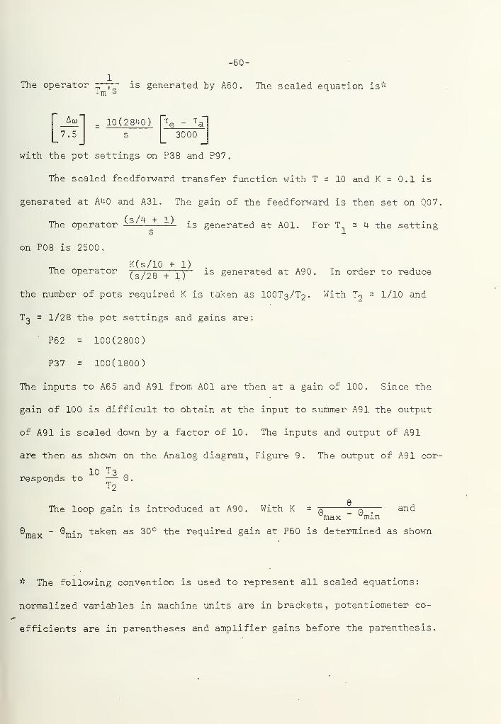
1The operator , is generated by A50. The scaled equation is»'-

"•m

7.5

10(2 840'I "^e - ^a13000s

with the pot settings on P38 and P97.

The scaled feedforward transfer function with T = 10 and K = 0.1 is

generated at A40 and A31. The gain of the feedforward is then set on Q07.

f s /4 + 1)The operator ^—^ is generated at AOl. For T, = 4 the setting

s 1

on P08 is 2500.

^ K(s/10 + 1) .

The operator(s/28 + 1)

"""^ generated at A90. In order to reduce

the number of pots required K is taken as IOOT3/T2. With Tj = 1/10 and

T3 = 1/2 8 the pot settings and gains are:

P62 = 100(2800)

P37 = 100(1800)

The inputs to A65 and A91 from AOl are then at a gain of 100. Since the

gain of 100 is difficult to obtain at the input to summer A91 the output

of A91 is scaled down by a factor of 10. The inputs and output of A91

are then as shown on the Analog diagram. Figure 9. The output of A91 cor-

responds to — 9.T2

aThe loop gain is introduced at A90. With K =

q q— and

max min

®niax~ ®min "t^^^s^ ^s 30° the required gain at P60 is determined as shown

* The following convention is used to represent all scaled equaticms:

normalized variables in machine units are in brackets, potentiometer co-

efficients are in parentheses and amplifier gains before the parenthesis,

-61-

below.

92.5 KtQ _ 92.50

-^e

"'^0 ®max ~ ®Tnin

utput of A91 is 10T̂2

10 T3 (gain) = 92.5

T2 ®max "'^min

(gain) 92.5 T2.8650

T3(0Tnax " ©min^

The required setting on P60 is then 1(8650).

LOAD COMPONENTS The induction motor speed is generated at A35.

The unsealed equation is: -„

The maximum motor speed is 1200 RPM which is the synchronous speed. The

maximum steady motor torque is approximately 1500 Ib-ft. Since the simu-

lated motor torque has the double frequency component the maximum torque

is twice the instantaneous D.C. level. As a result the maximum torque

is taken as 4000 Ib-ft. With the inertia (I) taken as 21.6 Ib-ft-sec^

the scaled equation becomes:

10(1475)[—

1

|_1200j4000 Set on P35

The propeller torque is generated at A63. The unsealed equation is

-^p = KpN^

_3With K = 1.08 X 10 and the torque and speed base values as above the

P

scaled equation becomes:

[

"^P

"

I- 1(3880) r__N^____l

4OOOJ |_i.44 X 10ej

Set on P67

-62-

The voltages and current in the simulation must be scaled based on

peak values rather than the RMS values. For maximum RMS values of 440

volts and I/phase of 1000 amps the base values are taken as:

^base = l^^l"^ ^"^Ps

Vbase 750 volts

Multiplier A3 3 generates the unsealed product of e and i. This is

scaled to the induction motor torque as follows. For the induction motor

for three phases

:

P(t) = 3 V^^^ sin(wt) Ijjj^j^ sin(wt + cf>)

or

^.^(t) = -^ ^max-'-iTiax (1 + cos2tot)'m 2WC

where the phase angle can be neglected in scaling the equation and (.7376)

is a conversion from newton-meters to Ib-ft. Wg is the synchronous me-

chanical speed which for this case is 125.6 rad/sec. With the base vari-

ables assumed above the scaled equation becomes:

h+oooI

= 10(2340)V

750

i

1414 Set on P35

The output of AOO must be scaled to Ijnax " 1^1'+ • The unsealed equa-

tion for AOO is :

1 = —s

1 (e -V )

Using the base values for current and voltage and the equivalent inductance

(L) for a single phase the scaled equation is:

|_1414j

10^ (8460) e - V

750

The motor voltage is generated at A03. The unsealed equation is:

V =RaIN

Ns-Ns. _ RI

1-N/Nc

-63-

The denominator is generated at A06 and is already in a non-dimensional

form. Scaling the equation for current and voltage gives:

r_vi ^ 1.89 R, r__oI 750J

1 - N/NsI

I^IM

The potentiometers in the switching network are then set to 1.89 R^ and

Ra' where R^ is the value for the rotor resistance and R^' the value of

the added rotor resistance.

The alternator torque is generated at multiplier A3 8. As shown

above this output can be scaled to a base torque of 4000 Ib-ft using the

same setting as on P35 which is 10(2340). However, the alternator torque

is filtered before being input to the gas turbine section so that it is

not necessary to scale this signal for the double frequency pulsation. With

the turbine base torque taken as 3000 Ib-ft the gain on the output of A38

is 10(3100). Since the second order filter is set to a gain of (1) this

gain is set on P07.

The scaled variables for all amplifiers and settings for all poten-

tiometers are given on the assignment sheets given in Tables 1 and 2.

-64-

Table 1.

AMPLIFIER ASSIGNMENTS

Amplifier

00

01

02

03

04

05

05

07

09

10

14

30

31

32

33

34

35

36

38

39

40

Scaled Value

i/1414

e/750

v/750

1.89R-,i/1414

CNs-N)/N

1^/3000

v/750

(v-e)/750

-(Ns-N)/N

-i/1414

vi/750 X 1414

-N^/1.44 X 10^

N/1200

dp -T^)/4000

Coimnent

Governor Control Box

Alternator Modulus

I.M. Back emf

For I.M. Back emf

Time Signal for ResistorNetwork

I.M. Slip

Invert I.M. Back emf

Invert A06

LPF for Viewing Torques

FFWD of Governor

I.M. Torque

I.M. Speed

Load Torque on G.T.

Governor Control Box

Governor FFWD Net

-55-

Amplifier Scaled Value Comment

44 Invert A02

50 Aa)/7.5 Change in Alternator Speed

51 Governor Error Signal

5 3 N^/1.44 X 10 For Propeller Torque

65 Governor Control Box

70 Butterworth Filter

74 Butterworth Filter

90 Tg/3000 G.T. Torque

91 Fuel Control Angle

95 Governor Control Box

100 Butterworth Filter

POT

Q04Q0700

020301+

05

07

08

10

32

34

35

36

37

38

60

6162

6465

6770

90

95

97

100

-66-

Table 2.

POTENTIOMETER ASSIGNMENTS

PARAMETER

Au/wq GainFFWD gain

Ra (switched)Alt. modulusRaSwitching timeTiming signalScale T^

Cont. box settingMotor inductanceRa (switched)Switching timeInertia of I.M.

Scale motor torqueGovt. Cont. boxAlt. inertiaControl loop gain

Butterworth filterGovt. Cont. boxSwitching time

Ra (switched)Scale propeller torque

Butterworth filterSwitching time

Ra (switched)Alt. inertiaButterworth filter

SETTING W/GAIN

1000 (10)2000 ( vary

)

6000Set for AG 7 outp0597117805003103 (10)

22878277 (1000)2000

32912000 (10)2341 (10)

1800 (10)

2841 (10)2177 (10) (vary)

5549 (100)

2651 (100)48952005

3880

8243

6 819

20012841 (10)5648 (100)

.8500

-67-

6. RESULTS

The results of monitoring the prototype performance and the results

of the simulation are shown on pages 59 through 75 . A chart speed of

twenty-five millimeters/second was used for all recordings. Strips A-L

correspond to a time duration of approximately fourteen seconds while

channels M-BB span approximately the first eight seconds of the simulation,

The records are presented in the following order.

A. Observed Alternator Speed Deviation

B. Simulated Alternator Speed Deviation

C. Observed K.W. Load (through 0.068 sec. LPF)

D. Simulated Alternator Torque (through 0.058 sec. LPF)

E. Observed Line Current

F. Simulated Line Current

G. Observed Induction Motor Speed (A.C. tachometer)

H. Simulated Induction Motor Speed

I. Simulated Motor Torque (through 0.068 sec. LPF)

J. Simulated Alternator Torque (through Butterworth filter)

K. Simulated Engine Torque - No Dead Time, No FFWD

L. Simulated Engine Torque - No Dead Tim.e , With FFWD

M. Alternator Speed with FFWD Gain (Q07) at .1000

N. Alternator Speed with FFWD Gain at .2000

0. Alternator Speed with FFWD Gain at .3000

P. Alternator Speed with FFWD Gain at .5000

-58-

Q. Simulated Output of Governor Load Sensing Section

R. Simulated Governor Error Signal

S. Observed Alternator Terminal Voltage

U. Simulated Alternator Speed with 0.1 Sec. Dead Time

V. Simulated Engine Torque with 0.1 Sec. Dead Time

W. Simulated Fuel Control Angle with 0.1 Sec. Dead Time

X. Simulated Alternator Speed with 0.01 Sec. Dead Time

Y. Simulated Engine Torque with 0.01 Sec. Dead Time

Z. Simulated Alternator Speed - Loop Gain = 1.0 Per Unit

AA. Simulated Alternator Speed - Loop Gain = 1.6 Per Unit

BB. Simulated Alternator Speed - Loop Gain =2.3 Per Unit

-69-

Figure 10lilv

CQSFffVEO ALTsBnaToh ERE<SOfcjjc> " .' lArjr oh;o

(— 1 SEC -^

If <AB/Jer y'Mu t. A-rfco Aixfert ^/AJ:o;i j"pe.6/> , ( D£\y /AT/oA^ EApj4 j^-A/cHSovoui _ y^ecTLX

"X,^

trwiB/stt }^i sec —

^

OQSfe/^veo K IV L.OA,D LtHIUo^h O.OtI I£C 4.Pf5^

/^

kr- I x*c -->|

S^ZlLV^A-ntQ <*i*.TfelJb/A-I50A__ XoaOWE jTtHRouSX Oq<,I J£t U>P")

-70-

_ Figure 10

. 9'}TA_^V£X> /AL0U.CT10V /lOTGA ^fego

k-l S4c—t

s//fv»sATte /vDucT/eAJ^ AieTx/t j"pefcP

*-j xec —jl

-71-

Figure 10

PE« uwiT flA^e I8*0 t.8- FT

I.O f.O.

;---; i-^ J^^J i L—t_L -1-4— i—i_L-

SiMOLAT-p^ Aure^x;^ ro^ rion qjtt.

PILR. wwrr 8-^s€ "Seoo ot PT

J^

SiMylLAT^^ EM<ilAJe__T[5«UlU£ Cw ITHOt/T Vfwn

C?OT » OOOO

SW^uuATeo ew&jM€. -ro<t.<i>ue fujiT<i Frwi(>

-72-

^t^*JLf\Tfn ACT S-P€fA - iTPuyn G-A/K) - . I

']

S/A^ciLA-nex» AO" SPe.g.0 — FFwa G-fi^i K) =. Jj.

O

0)

•H

S-if^ ULA-reX) /^CT S P€.<£.Q r* FFWQ ,C=f A/>0 - • -T

-73-

^/A>uCAT-<:0 Goi>ggX>0<^ ffwD 5

(JOl = aooo

S/HU LA-rer. -Bc x/^P-KiOR £/LfeQfk S«JJ a/ ,3J_

OQo*? =. aooo

OfiStJLv^ /KW^l^tJATOK Te^M/vAi. Woi-T/^ee

s^?5~P^

-74-

s/n^ft-AT^ n y^i^-|

^pg;€o - o.\ s^c n^Ao -riH€.

Qoi -= aooo CLf;VITt CORPOKAIION BRUSH INSIRUMENTS D

^iAlcrLATje.D__EVSriALS_jroA.9vjgi - O^l 5^C lOeADT/'MC

•

o

4)

oLS'iAlu<.Ar€£> AeroA-T^» A>J G-L£ - <^.l Sfcc 0£AD r//><g

(5on = aoOjO

S'J MULATTO AUr S"P6€£> — OOl S"^c 0«e>^C> T/>< g

QOl= llOOO

-75-

, ^:^Y^> ^:ri^-^>J^:)>u^_TgRj;^og^ O .o, 3-g^ n^AQ-nx£

--T-

:---^- -f-

! ! i

"'

"r:4:ri:t

Qoi - aooo

s^iM ULAT^o Ao- :!PE:gn -^oop gA/Aj - / PeiL UKjrr

o

0)

Oon - Q-poo

•^/McTLAre/o >\cr spe^^c - ^oop g^a/a) - /.C Po.

TE CORPORAnON BRUSH INSTRUMENTS DIVISION C^O 1 - 3 OOO

g/Hm-ATg^D >\Cr S-pCgLp - L.OQP Gf<i\J = ^.h Pu.

BB-

(S>OT •= ;0 00©tVliL COKPOt

-75-

DISCUSSION OF RESULTS

ALTERNATOR SPEED A comparison of strips A and B shows that there is

excellent qualitative correlation between the simulation and the prototype

performance. In the simulation the speed transient which occurs when the

induction motor switches to speed five occurs approximately one second too

late. This is due to an error in setting P90 which controls the switching

time for' motor speed five and in no way affects the validity of the model.

The three criteria listed below give an indication of the quantitative cor-

relation for the first speed transient.

(1) Maximum deviation in speed--For the prototype the drop in fre-

quency is eighteen chart divisions at a sensitivity of 20 mv/division. The

frequency converter sensitivity is 2.5V/5Hz. The frequency deviation is

0.72 Hz which corresponds to a 0.24 rev/sec drop in alternator speed. In

the simulation the speed drop was 1.5 rad/sec or 0.239 rev/sec.

(2) Ratio of speed drop to speed overshoot--Comparing the simulation

and prototype gives the following approximate values :

Simulation - 3.34

Prototype - 3.50

(3) Time to return to original speed—For both simulation and proto-

type the speed first returned to synchronous speed in approximately 0.70

seconds.

The correlation noted above is admittedly a retrofit to the prototype

data. However, it is clearly shown that the model used closely predicts

the prototype performance. In the simulation the engine parameters set

on the potentiometers were the values determined in the previous section.

-77-

The only settings which varied were the governor loop gain and the gain

on the governor feedforward signal. These two settings are varied in the

simulations to show their effects on engine performance.

The simulated output of the feedforward network is shown on strip Q.

As expected this signal shows the derivative operation in the FFWD net-

work. Strips M through P show the effect of increasing the FFWD gain.

On strip P the speed shows an initial increase when the load is applied.

This type of response is not possible for the system under study so that

an upper limit must be imposed on Q07 which corresponds to the FFWD gain.

However, the trend in engine performance as Q07 is increased is evident.

The effect of the FFWD on engine torque is shown in strips K and L.

The effect of loop gain on performance is shown in strips Z, AA and

BB. As gain is increased the speed deviations become smaller. In strips

AA and BB it is evident that the FFWD gain is set too high since the speed

shows a slight initial increase as load is applied. However, the influence

of loop gain is still clear.

In deriving the turbine model, the engine dead time was assumed to be

negligible or at least less than 0.01 seconds. The influence of dead time

on response is shown in strips U through Y. The dead time is simulated us-

ing a first order lag approximation. In strip U the speed response for 0.1

seconds dead time is shown. The response is noticeably worse than that

shown on strip N which is the response for the same potentiometer settings

for all components and with no dead time. The reason for the deterioration

in response is evident from comparing strips V and W. The dead time causes

the torque to lag the fuel actuator angle as shown. Strips X and Y corre-

spond to a dead time of 0.01 second. Comparison of the speed response

-78-

shown on strips X and N shows that there is no noticeable difference in

response. As a result, any dead time less than 0.01 second can be neglected.

ALTERNATOR LOAD Strip C is the alternator KW load as measured by the

governor load sensing section and as viewed through the 0.058 sec. LPF.

Since the maximum alternator speed variation is on the order of one percent

of base speed the load is roughly proportional to the alternator torque.

The load signal was not calibrated to a known level of load so that this

measurement may be used only for a qualitative comparison. Two ratios are

used below to give an indication of the degree of correlation. The over-

shoot ratio compares the maximum torque for each transient to the steady

torque level at the corresponding induction motor speed. The steady state

ratio compares the steady torque at each induction motor speed to the steady

torque at the maximum motor speed.

Table 3.

OVERSHOOT RATIO STEADY RATIO

IM SPEED

1

2

3

4 •

5

SIM

2.80

1.29

1.16

1.25

1.61

PROTO SIM PROTO

2.00 .47 .55

1.24 .65 .70

1.14 .72 .78

1.19 .84 .87

1.37 1.00 1.00

The differences between simulated and observed values is due primarily to the

difference between estimated and actual rotor resistance values.

A rough check can be made on the actual magnitude of the simulated

-79-

alternator torque. At speed five the induction motor torque is approximate-

ly 1400 Ib-ft at 1150 RPM. Since the alternator speed is approximately 1200

RPM and the power levels of the alternator and induction motor are approxi-

mately equal, the alternator torque will be approximately 1400 Ib-ft. The

scaled value for the simulated alternator torque is 1350 Ib-ft.

INDUCTION MOTOR The correlation of the induction motor performance

and the simulation is given in Table 4 below. The values for the motor

torque and current were taken from the motor performance curve. Figure 11 .

Also shown on this curve are the simulated values for torque and current.

Table 4.

Speed RPM RPM Torque ^RMS Torque ^RMS

Position Obs.

834

Sim.

840

(Performanc

800

:e Curve

)

Simulated

1 700 200

2 966 960 1000 310 915 250

3 10 32 1015 1100 340 10 30 275

4 1104 10 80 1270 380 1190 300

5 1180 1150 1450 425 1380 350

As with the engine simulation the results can vary widely depending on the

values used for the motor and propeller parameters. The original estimates

for the motor inertia and the rotor resistances were changed slightly in

order to provide a better fit between the model and the observed performance,

The differences between the original parameter estimates and the values used

in the simulation are summarized in Table 5.

80-

Table 5.

Estimated Setting FromParameter Value Potentiometer

PIG

Scaled Eqn.

8460(103)

Setting Used

^sm .71 ohms 8277(10^)

Ra .0117 P03 0220 0597

^a(l) .240 POO 4450 6000

Ra(2) .088 P32 1660 2000

Ra(3) .072 P65 1360 2000

Ra(U) .063 P95 1190 2000

Im+Ip 21.6 P35 1475(10) 2000(10)

K. 1.08 X 10"^ P67 3880 3880

All parameters agree with the estimated values except for the rotor

resistances and the motor inertia. The difference in inertia is not large

and is within the accuracy of the original estimate. The potentiometer

settings corresponding to values of R^ were considerably higher than the

original estimates. These higher settings result from the fact that a

single-phase model is being used to represent a three-phase machine.

For the three phase delta connected rotor the resistance is given as

0.0117 ohms. This resistance was probably measured across the slip rings

and would correspond to the following diagram.

As a result the single phase equivalent resistance (Rp) is 1.5 P^. This

requires that the settings for the potentiometers representing the rotor

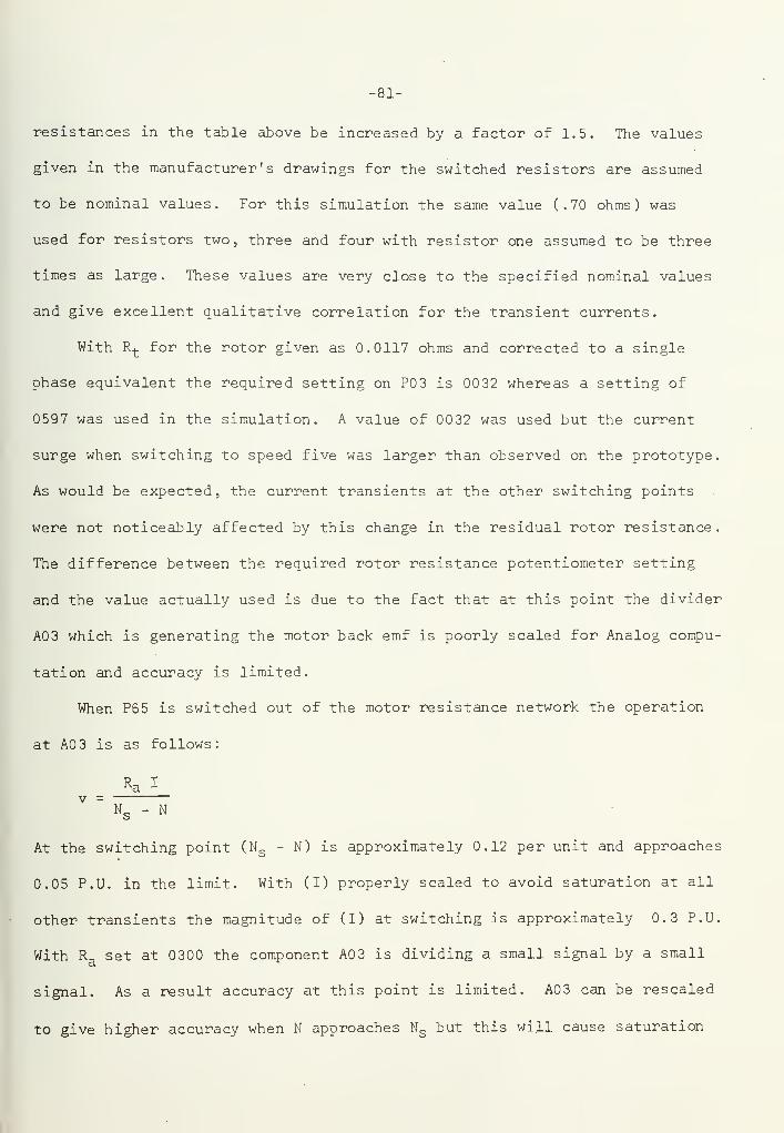
-81-

resistances in the table above be increased by a factor of 1.5. The values

given in the manufacturer's drawings for the switched resistors are assumed

to be nominal values. For this simulation the same value (.70 ohms) was

used for resistors two, three and four with resistor one assumed to be three

times as large. These values are very close to the specified nominal values

and give excellent qualitative correlation for the transient currents.

With R^ for the rotor given as 0.0117 ohms and corrected to a single

phase equivalent the required setting on P03 is 0032 whereas a setting of

0597 was used in the simulation. A value of 0032 was used but the current

surge when switching to speed five was larger than observed on the prototype.

As would be expected, the current transients at the other switching points

were not noticeably affected by this change in the residual rotor resistance.

The difference between the required rotor resistance potentiometer setting

and the value actually used is due to the fact that at this point the divider

A03 which is generating the motor back emf is poorly scaled for Analog compu-

tation and accuracy is limited.

When P65 is switched out of the motor resistance network the operation

at A0 3 is as follows:

Ra X

V =N3 - N

At the switching point (Ng - N) is approximately 0.12 per unit and approaches

0.05 P.U. in the limit. With (I) properly scaled to avoid saturation at all

other transients the magnitude of (I) at switching is approximately 0.3 P.U.

With Rg set at 0300 the component A03 is dividing a small signal by a small

signal. As a result accuracy at this point is limited. A03 can be rescaled

to give higher accuracy when N approaches Ng but this will cause saturation

-82-

when the motor is first started. The divider must be constrained to

operate at all times with the numerator smaller in magnitude than the

denominator.

Even with the reduced accuracy, when the motor speed approaches

synchronous speed, there is still good correlation between the simulation

and the prototype performance throughout the entire operating range.

Strips E through H show the correlation of speed and current. The data

tabulated above is plotted on the motor performance curve, Eigure 11, and

shows the quantitative correlation for torque and current. The simulated

current shows the same trend as the performance curve data but is lower at

all points. This is due in part to the error in measuring the magnitudes

of the current from the strip recording.

-84-

7. CONCLUSIONS AND RECOMMENDATIONS

The correlation between the simulation and prototype for all observed

variables proves the validity of the models used in the simulation. The

natural tendency is to expect that highly complex models will be required

for each component. However, reasonable accuracy in quantitative predic-

tions and highly valuable qualitative information about system performance

have been obtained using simple "off the shelf" models. The simulation

can be helpful in design or as a training aid.

As indicated earlier, the simulation gives the designer an indication

of trends in system performance as the various parameters are adjusted. For

a given motor the parameters X^^j, and R^ are fixed. The switched resistors

and switching times are the two most important parameters which can also be

easily adjusted. The simulation shows how the performance can be varied

over a wide range by adjusting these parameters. Although the designer has

little control over the inertia of the motor and propeller, the inertia ef-

fects are clearly shown. Finally, the effects of propeller pitch as char-

acterized by the propeller torque coefficient can be investigated.

The simulation provides an excellent study of the governing system

and engine performance. The most important governor adjustments are con-

trollable by potentiometer settings so that changes in the governor coef-

ficients can be investigated. The effects on engine torque and speed

response are clearly shown. In addition to providing useful design informa-

tion, the simulation can demonstrate to operating personnel the effects on

system performance due to changes in the governor settings

.

The transfer function approach to modeling the prime mover yielded a

-85-

simulation which can easily be adapted to any other type of prime mover by .

siibstituting the proper transfer function (on a diode function generator

if necessary) in the place of the gas turbine model. The model used in

this simulation is readily adaptable for use with diesel engines with the

most significant change being in the assumed engine dead time.

The two most important dynamic effects which were not included in the

simulation because of the limitation on computing hardware were the voltage

regulation and fuel control valve effects. With additional hardward these

effects can easily be included. However, as the results indicate, neglect

of these effects did not seriously affect the accuracy of the simulation.

Neglecting the stabilizer section of the governor control box and

dynamics of the fuel control valve did not seriously affect the results

for two reasons. The input disturbances to the gas turbine were below the

frequency level where the stabilizer section influences performance. Al-

though the load transient was close to a step change the second order filter

on load inputs to the gas turbine limits change to approximately 12 Hz. Al-

so, in scaling the simulation the developed engine torque was limited to

3000 Ib-ft. This provides a form of acceleration limiting.

Neglect of the voltage regulation effects can influence the results

in two ways. First, in the simulation the induction motor is supplied with

a constant voltage whereas in the prototype the voltage varies as shown in

Strip S. The error caused by this assumption is not serious. The second

effect of neglecting the voltage regulation is on alternator torque. With

field current assumed constant, the gyrator modulus on the alternator is

constant so that the torque is directly proportional to the line current.

-85-

The field ciorrent does Increase slightly during the transients so that the

prototype alternator torque is higher than shown on strip J. However, the

correlation between the simulation and prototype performance shows that

considering field current constant does not cause a serious error.

The use of a single-phase model for the three-phase machine intro-

duces no serious errors. The inertia of the induction motor is large

enough so that the double frequency torque pulsations in the motor are not

noticed. At the alternator end, the second order filter provided adequate

filtering of the pulsations and adequate frequency response in order to pass

the transient loads. Even with unlimited Analog hardware it would not be

necessary to use a three-phase model as the single-phase model is more than

.

adequate

.

RECOMMENDATIONS

The observed system performance indicates that the original system

design is more than adequate in order to meet its performance specifica-

tions. Therefore, use of this simulation in an attempt to improve the

overall design is not practical. The only change to the original system

which could be made at small cost is in the starting resistors. The speed

range of the motor with the installed resistors is from approximately 65

to 95 percent of synchronous speed. This range could be extended by chang-

ing the resistors. The required resistors and dynamic performance can be

determined by the simulation. However, it is not practical to lower the

speed significantly because then the motor will be operating at a very low

efficiency.

-87-

One area where additional work may be done is in utilizing the hybrid

capabilities of the computer facility. Although the simulation has been

done with only the Analog computer, the hybrid facility can be utilized to

increase the effectiveness of the simulation. One very interesting study

would be to perform an optimization study of the system. Even though

prototype system performance is adequate, such a study would give a student

the opportunity to learn the basics of hybria computing and to study in the

area of optimal control.

The most important dynamic elements which were neglected were the fuel

control valve and the voltage regulator. The governor control box stabilizer

section was also neglected. Since the simulation required approximately 90

.

percent of the Analog hardware, it would be difficult to include reliable

models of these components. A more detailed study of the generator set

alone can be performed by replacing the induction motor load by a step load

change. It will then be possible to include the effects of the fuel control

valve, voltage regulator and stabilizing section.

The generator set frequency regulation is extremely important for

proper operation of the shipboard electronic equipment. As a result, the

speed deviations of the gas turbine must be kept to a minimum when the

generator is supplying power to the electronic equipment. A simulation of

the generator set in response to step load changes can be used to design

the governing system and to determine the governor settings required for

best performance.

The most direct benefit of the simulation would be to use it to demon-

strate to operating personnel how the system performance can be altered by

adjusting the governor settings. The desire to "leave well enough alone"

-88-

together with a lack of complete understanding of how a system operates

will usually prevent operators from adjusting the governor to get better

performance. The simulation can be used to instruct operators in how the

various governor settings effect performance. With a better understanding

of how the system behaves, it will be easier to adjust the governor set-

tings for near optimum performance.

-89-

REFERENCES

(1) Paynter, H.M. , "Hydraulics by Analog— An Electronic Model of a

Pumpint Plant," J. Boston Soc. of Civil Engineers, July 1959, pp.197-219.

(2) Woodward Governor Company, "EG- A Control Box," Woodward Governor Company,Rockford, Illinois.

(3) EAI Inc. , Handbook of Analog Computation , published by ElectronicAssociates, Inc., 1967.

(4) EAI, Inc., 6 80 Reference Handbook, published by Electronic Asso-

ciates, Inc., 1967.

(5) Kamopp, D. and Rosenberg, R. , Analysis and Simulation of MultiportSystems

,published by the M.I.T. Press, 1968.

(6) Ferre, G. and Lenkaitis, D., "Gas Turbine Engine Analog Simulation forAcceleration Sensing Fuel Control Studies," from Gas Turbine Fuel Con-trols Analysis and Design, published by Society of Automotive Engineers,

• 1965.

(7) Del Toro, V., Principles of Electrical Engineering , published byPrentice-Hall, Inc., 1955.

(8) Paynter, H. , and Kamopp, D., "Design and Control of Multiport Engineer-ing Systems," Proceedings of IFAC Tokyo Symposium on Systems Engineeringfor Control System Design, 1965.

(9) Fitzgerald, A., and Kingsley, C. , Electric Machinery , published byMcGraw-Hill Book Company, 1961.

(10) "First Interim Technical Report, Computer Simulation of The Power Con-

version System for Nike-X Power Plants," 1 March to 15 July 1965,Arthur D. Little, Inc., Cambridge, Massachusetts.

Thesis 134737G86on Grosswei ler

Simulation and per-

formance analysis of

a shipboard gas tur-

bine emergency gen-

erator set.

thesG8605

Simulation and performance analysis of a""

mi

3 2768 002 13566 7DUDLEY KNOX LIBRARY