Embed Size (px)
Citation preview

Signals and Systems
Version 2.5 printed on February 2015 First published on March 2009
Signals & Systems Page 2
Background and Acknowledgements This material has been developed for the first course in Signal and Systems. The content is derived from the author’s educational, technical and management experiences, in-addition to teaching experience. Many other sources, including the following specific sources, have also informed the content and format of this text:
Nilsson, J. Electrical Circuits. (2004) Pearson. Oppenheim, A. Signals & Systems (1997) Prentice Hall Stremler, F. Introduction to Communication Systems (1990) Addison Lathi, B. Modern Digital and Analog Communication Systems (1998) Oxford University Press MathWorks. MATLAB Reference Material Version R2000a. (2007) MathWorks
I would like to give special thanks to my students and colleagues for their valued contributions in making this material a more effective learning tool. I invite the reader to forward any corrections, additional topics, examples and problems to me for future revisions. Thanks,
Izad Khormaee www.EngrCS.com
© 2010 Izad Khormaee, All Rights Reserved.

Signals & Systems Page 3
Contents
Chapter 1. Signals & Systems ...................................................................................................................... 5
1.1. Introductions .......................................................................................................................................... 6 1.2. Continuous-Time (CT) and Discrete-Time(DT) Signals ........................................................................ 8 1.3. Signal Energy and Power ................................................................................................................... 10 1.4. Independent Variable Transformations ............................................................................................... 12 1.5. Complex Exponential and Sinusoidal Signals .................................................................................... 16 1.6. Unit Impulse and Unit Step Functions ................................................................................................. 28 1.7. Fundamental System Properties ......................................................................................................... 33 1.8. Statistical Properties of Noise ............................................................................................................. 39 1.9. Chapter Summary ............................................................................................................................... 41 1.10. Additional Resources ........................................................................................................................ 42 1.11. Problems ........................................................................................................................................... 43
Chapter 2. Linear Time-Invariant (LTI) Systems ......................................................................................... 44
2.1. Linear Time Invariant (LTI) System Overview .................................................................................... 45 2.2. Convolution Sum in Discrete-Time LTI Systems ................................................................................. 46 2.3. Sidebar Notes (Useful Relationships) ................................................................................................. 53 2.4. Convolution Integral in Continuous-Time LTI Systems ....................................................................... 54 2.5. Linear Time-Invariant (LTI) Systems Properties ................................................................................. 58 2.6. Differential/Difference Equations ........................................................................................................ 62 2.7. Chapter Summary ............................................................................................................................... 65 2.8. Additional Resources .......................................................................................................................... 66 2.9. Problems ............................................................................................................................................. 67
Chapter 3. Fourier Series Representation of Periodic Signals ................................................................... 68
3.1. Overview & History of Fourier series .................................................................................................. 69 3.2. Complex Exponential Signals and LTI System Responses ................................................................ 70 3.3. Fourier Series Representation of Continuous-Time Periodic Signals ................................................ 74 3.4. Convergence of the Continuous-Time Fourier Series ........................................................................ 82 3.5. Continuous-Time Fourier Series Properties........................................................................................ 86 3.6. Fourier Series Representation of Discrete-Time Periodic Signals ..................................................... 90 3.7. Discrete-Time Fourier Series Properties ............................................................................................. 93 3.8. Application of Fourier Series in LTI systems ...................................................................................... 95 3.9. Chapter Summary ............................................................................................................................... 97 3.10. Additional Resources ........................................................................................................................ 98 3.11. Problems ........................................................................................................................................... 99
Chapter 4. The Continuous-Time Fourier Transform ................................................................................ 100
4.1. Introduction ....................................................................................................................................... 101 4.2. Fourier Transform for Aperiodic and Periodic Signals ...................................................................... 102 4.3. Fourier Transform Convergence ....................................................................................................... 106 4.4. Properties of the Continuous-Time Fourier Transform ..................................................................... 108 4.5. Chapter Summary ............................................................................................................................. 114 4.6. Additional Resources ........................................................................................................................ 115 4.7. Problems ........................................................................................................................................... 116
Chapter 5. The Discrete-Time Fourier transform ...................................................................................... 117
5.1. Introduction ....................................................................................................................................... 118 5.2. Fourier Transform of Aperiodic and Periodic Signals ....................................................................... 119

Signals & Systems Page 4
5.3. Fourier Transform Convergence ....................................................................................................... 123 5.4. Properties of the Discrete-Time Fourier Transform .......................................................................... 124 5.5. Summary of Fourier Series and Transform Equations ..................................................................... 129 5.6. Additional Resources ........................................................................................................................ 130 5.7. Problems ........................................................................................................................................... 131
Chapter 6. Sampling ................................................................................................................................. 132
6.1. Introduction ....................................................................................................................................... 133 6.2. Sampling Theorem ............................................................................................................................ 135 6.3. Aliasing Caused by Under Sampling ................................................................................................ 145 6.4. Interpolation Techniques for Signal Reconstruction From Samples ................................................. 148 6.5. Additional Resources ........................................................................................................................ 151 6.6. Problems ........................................................................................................................................... 152
Chapter 7. Communication Systems ........................................................................................................ 153
7.1. Introduction ....................................................................................................................................... 154 7.2. Amplitude Modulation (AM) ............................................................................................................... 157 7.3. Sinusoidal Amplitude Demodulation - Synchronous and Asynchronous .......................................... 162 7.4. Sinusoidal Frequency Modulation (FM) ............................................................................................ 167 7.5. Frequency-Division and Time-Division Multiplexing ......................................................................... 168 7.6. Common Modulation Techniques ..................................................................................................... 169 7.7. Additional Resources ........................................................................................................................ 170 7.8. Problems ........................................................................................................................................... 171
Chapter 8. Laplace Transform .................................................................................................................. 172
8.1. Laplace Transform “X(s) = Lx(t)” .................................................................................................... 173 8.2. Inverse Laplace Transform “x(t)=L-1x(t)” ......................................................................................... 175 8.3. Region Of Convergence (ROC) ........................................................................................................ 177 8.4. Laplace Transform Properties ........................................................................................................... 183 8.5. Application of Laplace Transform to LTI Systems ............................................................................ 185 8.6. Additional Resources ........................................................................................................................ 187 8.7. Problems ........................................................................................................................................... 188
Chapter 9. Z-Transform ............................................................................................................................. 189
9.1. Z-Transform, “X(z) = Zx[n]” ............................................................................................................. 190 9.2. Inverse Z-Transform, “x[n] = Z-1X(z)” .............................................................................................. 192 9.3. Region Of Convergence (ROC) ........................................................................................................ 193 9.4. Z-Transform Properties ..................................................................................................................... 197 9.5. Application of Z-Transform in LTI Systems ....................................................................................... 199 9.6. Additional Resources ........................................................................................................................ 200 9.7. Problems ........................................................................................................................................... 201
Appendix A. Additional Resources ............................................................................................................ 202

Signals & Systems Page 5
Chapter 1. Signals & Systems
Key Concepts and Overview Introduction
Continuous-Time (CT) and Discrete-Time (DT) Signals
Signal Energy and Power
Independent Variable Transformations
Complex Exponential Sinusoidal Signals
The Unit-Impulse and Unit Step Functions
Fundamental (CT & DT) System Properties
Statistical Properties of Noise
Additional Resources

Signals & Systems Page 6
1.1. Introductions
Study of signals and systems leverages mathematics, computer solutions, understanding of science and system engineering in order to analyze system behavior, design systems and derive information from signals. Signal and systems application can be found in a broad range of fields including:
Communication Aeronautics and Astronautics Circuit design Acoustics and visuals Seismology and Geology Biomedical Engineering Energy generation Distribution systems Chemical Process Control Speech Processing Financial Analysis and Forecasting
Although the underlying phenomenon or effect being studied in each field may be dramatically different, they all share two basic features:
Signals Signals are defined as functions that are dependent on one or more independent variables and carry information about the behavior or nature of one or more phenomenon. In this text we will focus on signals that depend only on a single independent variable. For example x(t). Although the dependent variable may vary, we will be using t as the default dependent variable.
Systems Systems are defined to respond to a particular signals by producing another signals which has a set of desired characteristics
Here are some examples of signals and systems applications:
Electrical Circuits Voltage value over time may be considered a signal x(t) Voltage or current in any other part of circuit may be used as system response y1(t) and y2(t)
Seismology
Signal may be the signal generated from the impact of some physical device with ground x(t) Response may be the reflection of signal as it bounces off different layers y(t)
R
L C Vi
+ Vo -
i + -
System x(t)
Input y(t) Response

Signals & Systems Page 7
Financial Market Economic parameters such as interest rate, earning, past price x1(t), x2(t), x2(t),… Output may be the future price of stocks y(t).
Most commonly signal and systems techniques are used to: Analyze and characterize existing systems Design systems to process signals based on a set of rules Enhance and restore signals Controlling characteristic of given systems based on input signals, system behavior and other
systems.
The remainder of this text provides a broad coverage of signal and systems with a focus on linear systems that are time invariant.

Signals & Systems Page 8
1.2. Continuous-Time (CT) and Discrete-Time(DT) Signals
As discussed earlier, the focus here is on signals with single independent variable. Further the default independent variable will be time, t. This enables the most efficient coverage of the topics but it is important to remember that the concepts may be applied to other signals with other types of independent variables. Natural phenomenon signals are continuous which means at any point time there is a value associated with the signal. This type of signal is referred to as continuous-time signal where the independent variable is continuous. For example, function x(t)=10sin(20t) represent a continuous function. In continuous-time, independent variable is represented by t (real number). In general continuous time signals are plotted with connected lines as shown below:
The second type of signal used in Signal & Systems is the Discrete-time signal where the independent variable only takes discrete values. Discrete-time signal allows for signal to be constructed out of discrete observed values. Each discrete value is a sample and we are not able of make any definite statements about the signal value between the sample points. In many cases, we make assumptions based on the underlying system characteristic in order to approximate the values between the sample points. x[n] is used to represent Discrete-Time signal (Note the use of “[“ instead of “(“ and “n” instead of “t”). n is an integer number. For example, function x[n] = 10 cos(10n) represent a discrete function. In general, discrete-time functions are plotted as stems:
Although we sense and effect our environment in continuous-time, efficiency of digital (computer) systems has encouraged the use of discrete-time to approximate and model systems. Digital systems are less expensive and more flexible in storing and processing system data. These facts have resulted in
x[n]
n 0 2
4 -2 -4 -6
x(t)
t 0
Signals & Systems Page 9
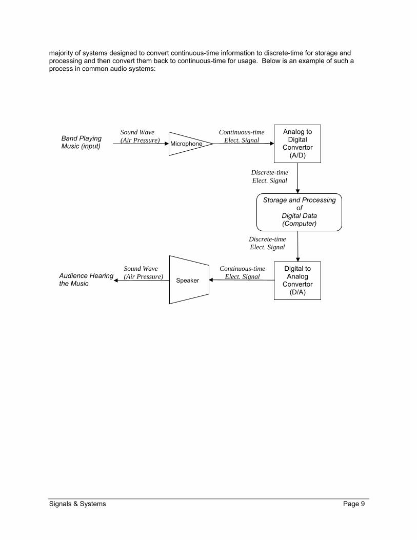
majority of systems designed to convert continuous-time information to discrete-time for storage and processing and then convert them back to continuous-time for usage. Below is an example of such a process in common audio systems:
Band Playing Music (input) Microphone
Analog to Digital
Convertor (A/D)
Storage and Processing of
Digital Data (Computer)
Digital to Analog
Convertor (D/A)
Audience Hearing the Music Speaker
Sound Wave (Air Pressure)
Continuous-time Elect. Signal
Discrete-time Elect. Signal
Discrete-time Elect. Signal
Continuous-time Elect. Signal
Sound Wave (Air Pressure)

Signals & Systems Page 10
1.3. Signal Energy and Power
In signals and systems, the first step is to relate the signals to the physical quantities. In electrical engineering, the focus is on power and by extension energy since power defines the ability of any electrical systems to effect change or sense change. In this section we will define three types of signals based on their energy profile. Note that for each concept introduced, it will be discussed with respect to Continuous-Time signal and with respect to Discrete-Time signal. In most cases, the two treatments will be similar but there are instances where the continuous (t) vs. discrete [n], effects the outcome. Let’s start from the basic concepts of Power (P) and Energy (E) in electrical engineering:
Power )(1
)()()( 2 tvR
titvtp
The total energy over the time interval 21 ttt
2
1
2
1
)(1
)( 2t
t
t
t
dttvR
dttpE
The average power over the time interval 21 ttt is represented by
2
1
2
1
)(11
)(1 2
1212
t
t
t
t
dttvRtt
dttptt
P
As discussed earlier, in the study of signal and systems, x(t) may be used to represent the magnitude of voltage therefore the energy equation for the discrete-time and continuous-time may be written as shown below:
Continuous-time Signal x(t) where |x(t)| is the amplitude of Complex value x(t)
The total energy over the time interval 21 ttt 2
1
2|)(|t
t
dttxE
The average power over the time interval 21 ttt
2
1
2
12
|)(|1
t
t
dttxtt
P
Discrete-time Signal x[n] where |x[n]| is the amplitude of Complex value x[n]
The total energy over the time interval 21 nnn
2
1
2|][|n
nn
nxE
The average power over the time interval 21 nnn
2
1
2
12
|][|1
1 n
nn
nxnn
P
Next, the above derivations may be extended by allowing the independent variables to approach :
Signals & Systems Page 11
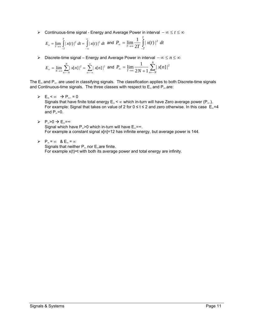
Continuous-time signal - Energy and Average Power in interval t
dttxdttxE
T
TT
22 |)(||)(|lim and
T
TT
dttxT
P 2|)(|2
1lim
Discrete-time signal – Energy and Average Power in interval n
n
N
NnN
nxnxE 22 |][||][|lim and
N
NnT
nxN
P 2|][|12
1lim
The E and P. are used in classifying signals. The classification applies to both Discrete-time signals and Continuous-time signals. The three classes with respect to E and P.are:
E < P. = 0 Signals that have finite total energy E < which in-turn will have Zero average power (P.). For example: Signal that takes on value of 2 for 0 ≤ t ≤ 2 and zero otherwise. In this case E=4 and P=0.
P>0 E=∞ Signal which have P>0 which in-turn will have E=∞. For example a constant signal x[n]=12 has infinite energy, but average power is 144.
P = & E = Signals that neither P nor Eare finite. For example x(t)=t with both its average power and total energy are infinity.

Signals & Systems Page 12
1.4. Independent Variable Transformations
It is common in signal and systems to transform a system’s response by transforming the independent variable (t or n). The three most common transformations used by engineers are time shift, time reversal and time scale. The remainder of this section will outline each of the three transformations and how they may be combined for a more complex transformation. As done earlier, each transformation is outlined for both discrete-time [n] and continuous-time t: Time Shift
Time Shift delays or advances the signal by adjusting the independent variable. x(t) x( t- t0)
If t0 > 0 the signal is delayed If t0 < 0 the signal is advanced
x[n] -> x[n - n0]
If n0 > 0 the signal is delayed If n0 < 0 the signal is advanced
Examples:
Time Reversal Time Reversal will reflect the signal about the origin with respect with independent. x(t) x( - t)
x[n] -> x[ - n]
Examples:
x(t)
t 0
x(-t)
t 0
x[n]
n 0 2 4
-2 -4 -6
x[n -2]
n 2 4 6
0 -2 -4

Signals & Systems Page 13
Time Scaling Time Scaling expands or compresses by multiply independent variables with a constant. x(t) x( at)
x[n] -> x[ an]
Examples-Scaling
Draw x(2t) for the following function, x(t):
Solution:
Example-Scaling Find the frequency of x(20t) when x(t) = 25 cos(1000πt). Solution: Student Exercise
General Form The above three transformations may be combined into a single step in the general form shown here: x(t) x( at+b)
x[n] -> x[an - b] where a & b are integers
x(2t)
t 0 2.5 -1.5
x(t)
t 0 5 -3

Signals & Systems Page 14
Example – Transformation Transform x(t) to x(5t/3 + 2) for the x(t) shown below.
Solution:
Note: This problem shifts first and scales second.
0 2 4 -2
1. x(t) Original Signal
2. x(t+2) shifted signal
t
0 2 4 -2
t
3. x(5t/3+2) scaled & shifted signal
0 6/5 2 -6/5
t
0 2 4 -2 t
x(t)

Signals & Systems Page 15
Example – Transformation
Transform x(t) to x(t/3 + 6) for the x(t) shown below.
Solution: (shift first and then scale)
Example – Transformation
Transform x(t) to x(3(t+4)) for the x(t) shown below.
Solution: Student Exercise
6 12 0 t
x(t)
2
-12 -6 3 -3 t
x(t/3+6)
20
15
2 4 7 5 t
x(t)
20
15

Signals & Systems Page 16
1.5. Complex Exponential and Sinusoidal Signals
This section introduces the most important signal class, Complex Exponential and Sinusoidal Signals that is the foundation of signal and systems analysis. The first step is to re-examine the definition of periodic signal for Continuous-Time and Discrete-Time:
Continuous-time periodic signal with period T x(t)=x(t+kT) Smallest positive T (real number) that satisfies the above equation is called the Fundamental
period T0.
Discrete-time periodic signal with period N x[n]=x(n+kN) Smallest positive N (integer) that satisfies the above equation is called the Fundamental
period N0.
One property that is utilized to simplify signal and systems analysis is Symmetry about the independent variable origin. A signal may have even, odd or mixed Symmetry:
Even Symmetry exists when: x(t) =x(-t) x[n]=x[-n] For example, function x(t) has even symmetry.
Odd Symmetry exists when: x(t) =-x(-t) x[n]=-x[-n]
Note: odd symmetric function by definition must be 0 at n=0 or t=0. For example, function x[n] has odd symmetry.
n
x[n]
2
4
5
-4-5
-2
-1 1 2 4 t
x(t)
-4 -2
Signals & Systems Page 17
Examples – Odd/Even Are Sin() and Cos() functions odd or even? Solution: Student Exercise
If a signal is neither odd nor even then must be a function with mixed symmetry. At times, it is useful to analyze the signal’s odd and even components independently. Below is the process to find the even and odd components of any signal:
Continuous-time Even x(t) = ½x(t) + x(-t) Odd x(t) = ½x(t) –x(-t)
Discrete-time
Even x[n] = ½x[n] + x[-n] Odd x[n] = ½x[n] –x[-n]
For example, x(t) = 2t + 1 is neither purely even nor purely odd but has mixed symmetry. Here is the process to find the even and odd parts of this mixed signal: Even x(t) = ½x(t) + x(-t) = ½ 2t +1 -2t +1 = 1 Odd x(t) = ½x(t) –x(-t) = ½ 2t + 1 +2t -1 = 2t

Signals & Systems Page 18
Examples – Odd/Even Part
Find odd and even part of X[n]
Solution: Student Exercise
Examples – Odd/Even Part Find odd and even part of the following function: x(t) = 3t + cos(t) Solution: Student Exercise
n
x[n]
2
4
-4
-2 -1 0 1 2 3
-2

Signals & Systems Page 19
Now that we have the definition for periodic signals and symmetry, we are ready to introduce the Complex Exponential and Sinusoidal Signal classes. This class of signals is the basis of signal definition throughout this text and is the most common approach to signal definition in the industry. These signals serve as a basic building block of many common signals. This section covers the Continuous-Time(CT) first, followed by Discrete-Time(DT) classes of Complex Exponential Sinusoidal Signals. Continuous-Time Complex Exponential Sinusoidal Signals
The general form of Complex Exponential and Sinusoidal is best stated by the following:
atCetx )( Where C and a are both complex numbers
imagrealj jaaeaa a ||
imagrealj jCCeCC c ||
The simplest form of x(t) is when a=0 which resolves x(t) to simple constant value. The next simplest form of x(t) occurs when both a and C are real. In this case x(t) resolves to real exponential signal. Depending on the sign of a, x(t) may be growing and decaying exponential as shown below:
Another subclass of signals are when “a” is pure imaginary which results in:
tjwetx 0)( Complex Periodic Exponential.
The Complex Periodic Exponential signals have a number of important properties which are listed below: Periodicity
Of course this signal is periodic which means:
)(00)( Ttjwtjw eetx Where
0
0
2
wT
is fundamental period and T is multiple of T0
Here is the proof that the above equality is true:
x(t)
t
C
x(t) has the exponential decay form when (a<0)
x(t)
t
C
x(t) has the exponential growth when (a>0)

Signals & Systems Page 20
tjwTtjw
Tjw
Tjw
TjwtjwTtjw
eetx
jethenw
nTSince
TwjTwelationsEulerapply
eeetx
00
0
0
000
)(
0
00
)(
)(
1012
sincosRe'
)(
Sinusoidal Signal
The Sinusoidal Signal )cos()( 0 twAtx is closely related to Complex Periodic Exponential
(Real part of the signal) which is demonstrated below using Euler’s Relation:
Im)sin(
Re)cos(
:22
)cos()(
sincosRe':
)(0
)(0
0
0
0
00
tjw
tjw
tjwjtjwj
jb
eanginaryAtwA
ealAtwA
itwritetowayAnother
eeA
eeA
twAtx
bjbelationsEulerNote
Average Power and Total Energy
Use the Average Power and Total Energy equations to calculate the corresponding for Complex
Periodic Exponential signal tjwetx 0)( .
12
||2
1|)(|
2
1lim 22 0
T
TTdte
Tdttx
TP
T
T
tjwT
TT
dtedttxE tjw 22 |||)(| 0
Note: 1|||)(| 0 tjwetx ; to prove this equality use Euler’s Identity "sincos" ajae ja .
Finally, the General form of Complex Period Exponential Signals atCetx )( Where:
jeCC || C is complex represented in Polar Form
0jwra a is complex represented in Rectangular Form
The above relationships may be used to rewrite atCetx )( in a form that we are more familiar
with, using Euler’s Identity:
)sin(||)cos(||)(
||||)(
00
)()( 00
tweCjtweCtx
eeCeeCCetxrtrt
twjrttjwrtat
Below are the graphical representations of Real Part of x(t) (imaginary is ignored):

Signals & Systems Page 21
Example – Complex Exponential Signals
Given the ability to generate complex exponential signal, x(t)=Ceat, show how you can generated cos(wt) signal. Note: a and C are complex numbers and you may utilize Euler’s Identity. Solution:
x(t)
t
r=0 “a is pure imaginary” x(t)=|C|cos(w0t + ) Constant Sinusoidal Signal
x(t)
t
r>0 x(t)=|C|ertcos(w0t + ) Growing Sinusoidal Signal
x(t)
t
r<0 x(t)=|C|ertcos(w0t + ) Decaying Sinusoid Signal damped sinusoid- RLC Circuit
Signals & Systems Page 22
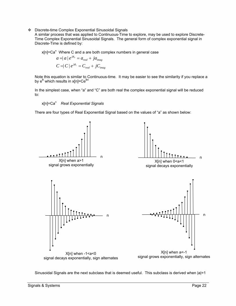
Discrete-time Complex Exponential Sinusoidal Signals A similar process that was applied to Continuous-Time to explore, may be used to explore Discrete-Time Complex Exponential Sinusoidal Signals. The general form of complex exponential signal in Discrete-Time is defined by: x[n]=Can Where C and a are both complex numbers in general case
imagrealj jaaeaa a ||
imagrealj jCCeCC c ||
Note this equation is similar to Continuous-time. It may be easier to see the similarity if you replace a by eB which results in x[n]=CeBn In the simplest case, when “a” and “C” are both real the complex exponential signal will be reduced to: x[n]=Can Real Exponential Signals There are four types of Real Exponential Signal based on the values of “a” as shown below:
Sinusoidal Signals are the next subclass that is deemed useful. This subclass is derived when |a|=1
n
n
n X[n] when a>1
signal grows exponentially X[n] when 0<a<1
signal decays exponentially
X[n] when a<-1 signal grows exponentially, sign alternates
n
X[n] when -1<a<0 signal decays exponentially, sign alternates

Signals & Systems Page 23
and B is pure imaginary (B=jwon) as shown below:
njwCenx 0][ Sinusoidal Signals
Using Euler’s identify, we can rewrite the above equation in term of complex exponential by:
njwjnjwj eeA
eeA
nwA 00
22)cos( 0
Now is the time to explore general form of Complex Exponential Periodic Signals in Discrete-Time. First, let’s rewrite the General Complex Exponential Signals in order to interpret it in-term real exponential and sinusoidal signals. Apply the polar form of C and a to X[n] general form equation:
)sin(||||)cos(||||][
||&||
00
0
nwaCjnwaCCanx
eaaeCCnnn
jwj
The above general form may be represented by one of the following three graphs based on the range of “a” values.
n
x(t) when |a| > 1 “Sinusoidal Multiplied by growing exponentials”
n
x(t) when |a| = 1 “Real & imaginary part of complex exponential are sinusoidal”

Signals & Systems Page 24
Discrete-time has similar periodic properties as Continuous-Time but there are also important
distinctions. The exponential signal with frequency wo is the same as any signal with frequencies (wo + 2k) where k is an integer:
njwnjnjwnwj eeee 000 2)2( Real part or Cos(w0n) is typically plotted.
Although any 2 period may be used to as the period, commonly intervals 20 0 w or
0w are used.
A few additional points to consider: wo at 2n and 0 which produce the lowest rate of oscillation:
102 jj ee
wo at n produces the highest number of oscillations njne )1(
x[n]= njwe 0 is periodic with period N only if woN is a multiple of 2. It is important to note that unlike the Continuous-Time, woN is not guaranteed to be a multiple
n
N =2 sample Period w0 = 2/N = x[n]=cos(n)
…
n
N =1 sample Period w0 = 2/N = 2 x[n]=cos(2n)=cos(0)
…
n
x(t) when |a| < 1 “Sinusoidal multiplied by decaying exponentials”

Signals & Systems Page 25
of 2. Therefore we need to ensure it is true when analyzing a signal. Starting with the definition of periodicity. IN order for x[n] to be periodic with period N, it must satisfy:
)(00
Nnjwnjw ee For this equation to be true,
equation mjNjw ee 210 must hold true
Which means mNw 20
therefore
fundamental frequency. N
mw
20
fundamental period is )2
(0w
mN
when integers m and N have no common factors
Finally, note that 20w
must be rational number for signal njwe 0 to be periodic.
Examples – Fundamental Period and Frequency
Example – Find the fundamental period and frequency of the following Discrete-Time signals:
Solution: N =12 Sample Period w0 = 2/N = /6 x[n]=cos(n/6)
Example – Find the fundamental period and frequency of the following Discrete-Time signals:
Solution: N =8 Sample Period w0 = 2/N = /4
n
…
n
…

Signals & Systems Page 26
x[n]=cos(n/4)
Example – what is the fundamental frequency and period of the combined discrete-time signals represented by the following equation:
njnj eenx )6/2()8/4(][
Solution: First term has fundamental period N1=4 Second term has fundamental period N2=6 x[n] fundamental period, N, is the lowest common multiplier by N1 & N2 N = 12 (evenly divisible to both terms fundamental period)
Signals & Systems Page 27
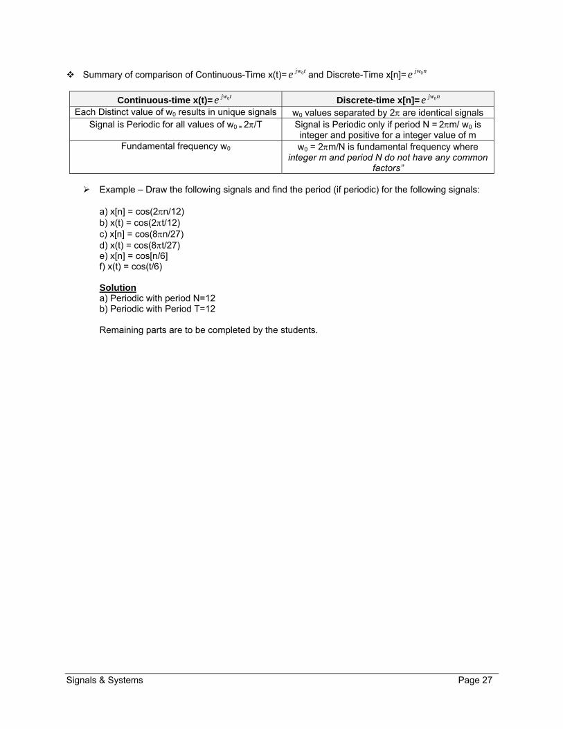
Summary of comparison of Continuous-Time x(t)= tjwe 0 and Discrete-Time x[n]= njwe 0
Continuous-time x(t)= tjwe 0 Discrete-time x[n]= njwe 0 Each Distinct value of w0 results in unique signals w0 values separated by 2 are identical signals
Signal is Periodic for all values of w0 = 2/T Signal is Periodic only if period N = 2m/ w0 is integer and positive for a integer value of m
Fundamental frequency w0 w0 = 2m/N is fundamental frequency where integer m and period N do not have any common
factors” Example – Draw the following signals and find the period (if periodic) for the following signals:
a) x[n] = cos(2n/12) b) x(t) = cos(2t/12) c) x[n] = cos(8n/27) d) x(t) = cos(8t/27) e) x[n] = cos[n/6] f) x(t) = cos(t/6) Solution a) Periodic with period N=12 b) Periodic with Period T=12 Remaining parts are to be completed by the students.

Signals & Systems Page 28
1.6. Unit Impulse and Unit Step Functions
Unit Impulse and Unit Step functions are two ideal signals specially defined as a tool for signal processing. Both signals are crucial in our ability to model systems mathematically. In this section we will define these functions. Discrete-Time Unit Impulse and Unit Step Function
Unit impulse, [n] (or unit sample)
Unit impulse is equal to 1 only when the independent variable is equal to 0; otherwise unit impulse is 0.
Here are a couple of relationships that explain the reason for also referring to impulse function as sample function.
n
[0]x = [n] x[0]= [n]x[n]
To prove refer to the definition of [n] which says [n] is only 1 at n=0 The more general form of the above equation is shown below:
n
][nx = ]n-[n] x[n= ]n-[nx[n] 0000
Unit impulse is commonly referred to simply as impulse function.
Unit Step function, u[n] Step response is equal to 1 as long as the independent variable is larger or equal to 0.
It is commonly referred to Unit Step function as simply Step function.
Relationships between Step and Impulse functions * From Step to Impulse function conversion . [n]=u[n]-u[n-1] * From Impulse to Step Function conversion
1
0
u[n] 0,1
0,0
n
n
n
. . .
1
0
[n] 0,1
0,0
n
n
n “Greek character Delta”

Signals & Systems Page 29
u[n]=
0
][k
kn
Example - write the following function in term of step functions and then again in terms of
impulse function.
Solution: Step Function Representation: x[n] = 6u[t] - 6u[t-5] Impulse Function Representation: x[n]= 6 [0] + [1] + [2] + [3] + [4]
Example - write the following function in term of step functions.
Solution: <Student Exercise>
Continuous-time Unit Impulse and Unit Step Response
Unit impulse, (t) (or unit sample)
Unit Impulse function has no duration but the unit area is 1.
Unit impulse is commonly referred to simply as impulse function. Impulse function is also used to sample value of a continuous function utilizing the following property of impulse function:
1
0
(t) 0,1
0,0
t
t
t
(t)
n0 1 2 3 4
4
-10 -9 -8
n0 1 2 3 4
6

Signals & Systems Page 30
x(0))()x(
d
This is true based on definition of (t) which say it is only 1 at t=0 Here is a more general form:
)x(t)()x()()x( 0000
tttdt
Unit Step, u(t) function
Step function is equal to 1 when t>0 and is equal otherwise. Step function is undefined at t=0.
Unit Step function is commonly referred to simply as impulse function
Relationship between Impulse and Unit Functions Impulse function may be written in-term of Unit Step Function using the following relationship:
dt
tdut
)()(
Below is the graphical representation:
Another approach is to write Unit Step function in-term of Impulse Function using:
0
)()( dtu
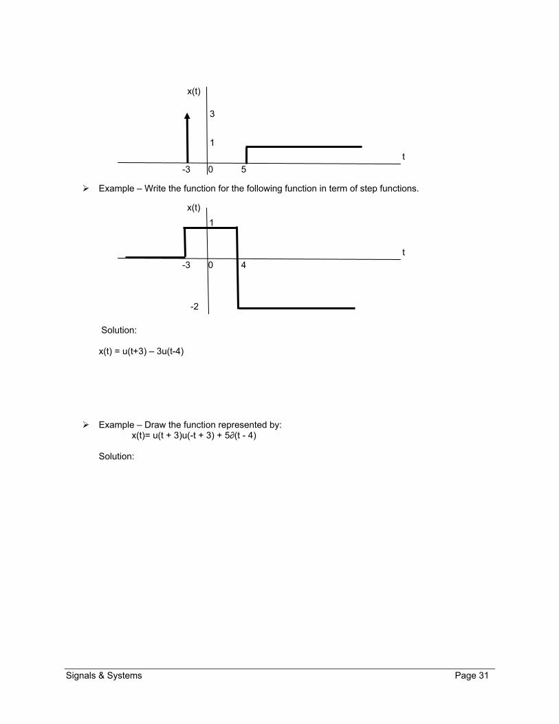
Example – Draw the function x(t)=u(t-5) + 3(t+3).
Solution:
1
0
t
u(t) where 0
1/
0
t
(t) where 0
1
0
u[t] 0,1
0,0
t
t
t
Signals & Systems Page 31
Example – Write the function for the following function in term of step functions.
Solution: x(t) = u(t+3) – 3u(t-4)
Example – Draw the function represented by: x(t)= u(t + 3)u(-t + 3) + 5∂(t - 4) Solution:
1
-3 0 4
t
x(t)
-2
3
1
-3 0 5
t
x(t)
Signals & Systems Page 32
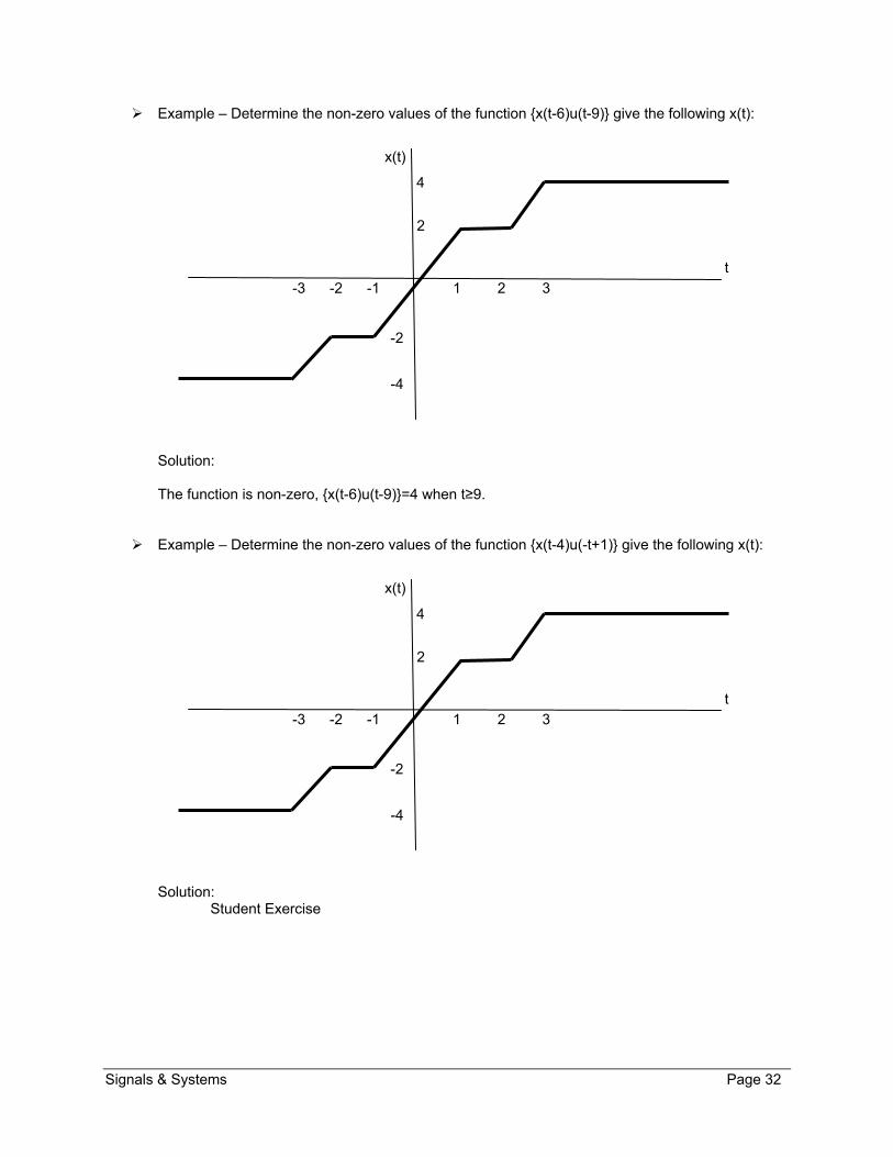
Example – Determine the non-zero values of the function x(t-6)u(t-9) give the following x(t):
Solution: The function is non-zero, x(t-6)u(t-9)=4 when t≥9.
Example – Determine the non-zero values of the function x(t-4)u(-t+1) give the following x(t):
Solution: Student Exercise
2
-3 -2 -1 1 2 3
t
x(t)
-2
4
-4
2
-3 -2 -1 1 2 3
t
x(t)
-2
4
-4

Signals & Systems Page 33
1.7. Fundamental System Properties
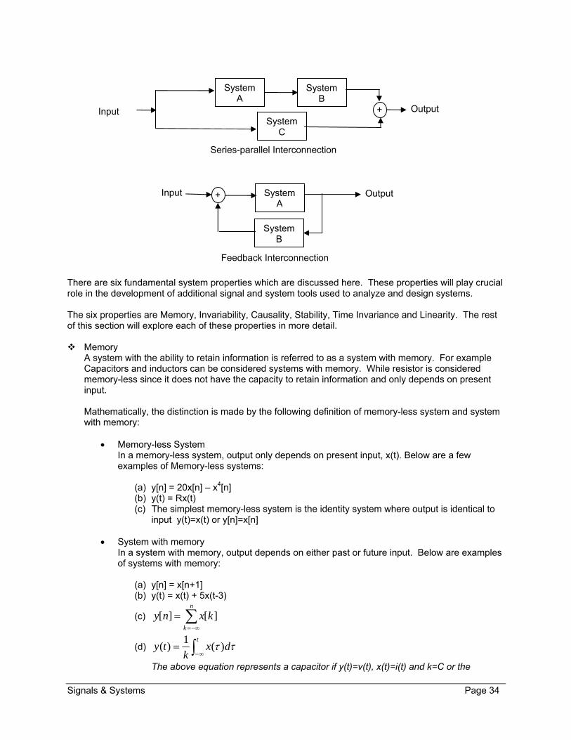
As it was discussed earlier the concept of signal and systems applied to a broad range of fields beyond Electrical Engineering. The power of signal and system comes from the fact that all problems to be solved or analyzed can be modeled as a system. A System is a mathematical model of physical systems that has a set of inputs and outputs. It additionally describes a transformation from the input to output signals. A system diagram for fully discrete-time or fully continuous-time is shown below:
More complex systems can be designed by interconnection systems in order to perform more complex tasks. Systems are typically interconnected in one of the following four configurations:
System A
System B
Parallel Interconnection
Input + Output
System A
System B
Cascade (Series) Interconnection
Input Output
Continuous-time System
Discrete-time System x[n]
y(t) X(t)
y[n]
Signals & Systems Page 34
There are six fundamental system properties which are discussed here. These properties will play crucial role in the development of additional signal and system tools used to analyze and design systems. The six properties are Memory, Invariability, Causality, Stability, Time Invariance and Linearity. The rest of this section will explore each of these properties in more detail. Memory
A system with the ability to retain information is referred to as a system with memory. For example Capacitors and inductors can be considered systems with memory. While resistor is considered memory-less since it does not have the capacity to retain information and only depends on present input. Mathematically, the distinction is made by the following definition of memory-less system and system with memory:
Memory-less System In a memory-less system, output only depends on present input, x(t). Below are a few examples of Memory-less systems:
(a) y[n] = 20x[n] – x4[n] (b) y(t) = Rx(t) (c) The simplest memory-less system is the identity system where output is identical to
input y(t)=x(t) or y[n]=x[n]
System with memory In a system with memory, output depends on either past or future input. Below are examples of systems with memory:
(a) y[n] = x[n+1] (b) y(t) = x(t) + 5x(t-3)
(c)
n
k
kxny ][][
(d)
tdx
kty )(
1)(
The above equation represents a capacitor if y(t)=v(t), x(t)=i(t) and k=C or the
System A
System B
Feedback Interconnection
Input + Output
System B
System C
Series-parallel Interconnection
Input + Output
System A

Signals & Systems Page 35
equation represents an inductor if y(t)=i(t), x(t)=v(t) and k=L.
Invertibility A system is invertible if the system generates unique output in response to a unique input. In this type of systems, output may be used to uniquely identify the input which is the benefit of Invertibility. In a invertible system, an inverse system exists such that when cascaded with the original system, the output of the combined system, w[n] is the same as the input x[n]
For example y[n]=3 is not invertible since there is no way to identify a unique input on the other hand y(t) = 4x(t) is invertible since input is uniquely related to the output. The system described by y(t)=x2(t) is not invertible since the sign of input is lost therefore input cannot be uniquely identified based on output. The concept of Invertibility is key to any system that takes an input that needs to be recovered at some point in the future. For example cell phones and computers. Can you think of any other ones?
Causality A system is causal if the output depends only on present and past input. The causal system does not anticipate input which is the reason it is also called no anticipative system. On the flip side, a non-causal system depends on the future input. Example - Is the system described by y[n]=x[n]+x[n+3] Causal?
Solution: The system is non-causal since it depends on x[n+3] which is a future input.
Example - Is the system described by y[n]= x[-n] Causal? Solution: Before answering try n=-2 note that y[-2]=x[2] is noncausal
Example - Is the system described by y(t)=x(t)sin(t+2) Causal? Solution: Yes, since it only depends on current x(t). Note that sin(t+2) is just a factor and has nothing to do with the input. The concept of causality is a valuable concept in speech, image processing as well as geographical/meteorological signals.
Stability A Stable system is one in which small inputs lead to responses that do not diverge. An example of a stable physical system is a ball sitting at the bottom of inverted cone. On the other hand if the ball is balance on top of a cone, it is unstable since the slightest force will dislodge the ball from the top. In general, stability of physical systems results from the presence of mechanisms that dissipate energy. A system is said to be stable if the system output is bounded in response to all bounded input. In other words, if the input is finite (|x(t)|<∞) then the output also will be finite. Example - Is the system described by y(t)=tx(t) stable?
Solution: The system is unstable since for bounded x(t) y(t) is unbounded as
y(t) = 5x(t) w(t) = (1/5) x(t) x(t) y(t)
w(t)=x(t) System Inverse System
Signals & Systems Page 36
t approaches infinity.
Example - Is the system described by y(t)= ex(t) stable? Solution: The system is stable since y(t) is bounded as long as x(t) is bounded.
Time Invariance A system is time invariant if the system characteristic does not change over time. For example a typical RLC circuit is time invariant since its behavior does not change for one minute to the next. The formal definition is that a system is time invariant if an input shift-in-time results in an identical time-shift in the output. Example - Is the system described by y(t)=5 cos[x(t)] time invariant?
Solution: First apply the input x1(t) to the system y1(t)=5cos[x1(t)] and shift by t0 y1(t-t0)=5cos[x1(t-t0)] Second apply the time shifted input x2(t) = x1(t-t0) to the system y2(t)=5cos[x1(t-t0)] . Since y1(t- t0) = y2(t) then the system is time invariant.
Example: Is the system described by y[n]=2nx[n] time invariant? Solution: Using the formal approach… First apply the input x1[n] to the system y1[n]=2nx[n] and shift by n0 y1[n-n0]=2(n-n0)x1[n-n0] Second apply the time shifted input x2[n] = x1[n-n0] to the system y2(t)=2n x1[n-n0] . Since y1(t- t0) ≠ y2(t) then the system is not a time invariant system. Alternative approach - Sometime it is easier to find one input that violates the time invariant rule such as is done below: 1) set x1[n]=[n] y1[n]=n[n]=0 always (Hint: [n]=1 only if n=0) 2) set x2[n]= [n-1] y2[n]=n[n-1]= [n-1] Since y2[n] from shifted input is not equal to shift output y1[n-1] then this is not a time invariant system.
Example: Is the system described by y(t)=x(t + 2) time invariant? Solution:

Signals & Systems Page 37
Linearity A linear system exhibits the superposition property which defines linearity. The superposition has the following two characteristics: 1) Additive Characteristic response to x1(t) + x2(t) is y1(t) + y2(t) 1) Homogeneity Characteristic response to ax1(t) is ay1(t) where a is any complex constant Both of the characteristics can be combined to a single statement which may be state for CT and DT as shown below: Continuous-Time (CT): ax1(t) + bx2(t) ay1(t) + by2(t) Discrete-Time (DT): ax1[n] + bx2[n] ay1[n] + by2[n] Note: a and b can be complex numbers. The Superposition property statements can be generalized to:
Continuous-Time (CT): k
kkk
kk tyatytxatx )()()()(
Discrete-Time (DT): k
kkk
kk nyanynxanx ][][][][
Example - Is the system described by y(t)=tx(t) linear?
Solution Apply x1(t) y1(t)=tx1(t) Apply x2(t) y2(t)=tx2(t) x3(t)= ax1(t) + bx2(t) y3(t)=tax1(t) + bx2(t) Since y3(t) = ay1(t) + by2(t), This is a linear system.
Example - Define the properties of a system where x(t) is the input and y(t) is the output as defined below: a) y(t) = 2t + 1 b) y(t) = 2x(t) +1 c) y(t) = t2 + x(t+1) d) y(t) = (t-1)x(t) Solution Student Exercise.
Note if y3(t) = ay1(t) + by2(t) Then “a linear system” Else “Not a linear system”

Signals & Systems Page 38
Example - Define the properties of a system where x[n] is the input and y[n] is the output as defined below: a) y[n] = x[n] b) y[n]=x[n+1] c) y[n] = x[n]x[n-2]
d)
0
0
][][nn
nnk
kxny
Solution Student Exercise.
Example - Define the properties of a system where x[n] is the input and y[n] is the output as defined below: y[n] = cos[w0n + ] x[-n + 3]u[-5 + n] – u[n - 9] Solution Student Exercise.

Signals & Systems Page 39
1.8. Statistical Properties of Noise
Discussion of signal and system is not complete without an overview of noise in the system. As the name implies noise is an unplanned, unwanted and in many cases an unknown quantity in the system. Noise may have been introduced to the system from other devices, natural phenomenon or the system itself. The goal of designer is to be able to separate the signal which carries the information even in a noisy environment. In cases where Noise is understood and has a well define characteristic, then it may be filtered out but when the noise is distributed over a range and has a random nature then a broad solution is need based on the profile of noise. The most common approach to understanding and treatment this type noise is through probabilities and statistics. In this section we will introduce one of the most common noise classes which are the white noise. White noise is a random signal which is distributed with a uniform, Gaussian or other probability distributions. Before discussing an example of white noise distribution, let’s start with the definition of probability distribution. In statistics, a probability distribution is defined as:
the probability of occurrence of any value of an unidentified random variable for Discreet-Time. the probability of occurrence of any value falling within a particular interval for Continuous-time.
The most common type white noise is the uniformly distributed white noise which is a random signal with a uniformly distributed value distribute between two frequencies. Discrete Uniform Distribution
Discrete Uniform Distribution is a discrete probability distribution that allows all values of a finite set equal probability of occurring. Let’s say the set of possibilities are AA1, A2, … An) and they are distribution uniformallly. At any given point, each possibility (Ai) has probability equal to (1/n) to be present. In Matlab such a discrete uniformally distributed white noise may be created by the use of random number generator that is limited to the list of possibilities.
Continuous Uniform Distribution Continuous Uniform Distribution is a probability distribution where each value in a given range has equal probability of occurring. Below is the probability function:
Probability Density Function
t Min Max
1/(Max –Min)

Signals & Systems Page 40
MaxtorMintwhen
MaxtMinwhenMinMaxtp
0
1)(
The uniformally distributed white noise plays an important role since it allows testing of design to verify that the signal can be recovered when noise is present at a given range of frequencies. The random nature forces designer to solutions other than filter which are static in their basic implementation. Signal and Noise is an integral part of signal and systems student so will be encountering them again.

Signals & Systems Page 41
1.9. Chapter Summary

Signals & Systems Page 42
1.10. Additional Resources
Oppenheim, A. Signals & Systems (1997) Prentice Hall
Chapter 1.
Modern Digital & Analog Communication Systems (1998) Oxford University Press Chapter 2
Stremler, F. Introduction to Communication Systems (1990) Addison-Wesley Publishing Company Chapt 2
Introduction to Statistics

Signals & Systems Page 43
1.11. Problems
Refer to www.EngrCS.com or online course page for complete solved and unsolved problem set.
Signals & Systems Page 44
Chapter 2. Linear Time-Invariant (LTI) Systems
Key Concepts and Overview Linear Time Invariant (LTI) System Overview
Convolution Sum in Discrete-Time LTI Systems
Convolution Integral in Continuous-Time LTI Systems:
LTI Systems Properties
Differential/Difference Equations
Additional Resources

Signals & Systems Page 45
2.1. Linear Time Invariant (LTI) System Overview
Fundamentals of signals and systems were introduced in previous chapter. In this chapter, the focus is on defining Linear Time Invariant (LTI) systems which serve as the start point for modeling systems. LTI systems also are the foundation for the topics covered in the next chapters. Linear Time Invariant systems as the name implies have two defining properties:
Linearity In a linear system superposition hold true which means responses to individual input can be summed up to calculate the total system response.
Time-invariance Time-invariance provides for shifting input in time and expecting output to shift in time without changing its characteristic.
The following sections explore the concepts of system impulse response, convolution sum/integration, and difference/differential equations for both the Discrete-Time and Continuous-Time Linear Time Invariant (LTI) systems.

Signals & Systems Page 46
2.2. Convolution Sum in Discrete-Time LTI Systems
Any signal may be describe using impulse functions as discussed in the previous chapter. In general any signal can be written as:
][][][
...]2[]2[]1[]1[][]0[]1[]1[...][
knkxnx
nxnxnxnxnx
k
This equation is built based on the fact that impulse function can be used to isolate (or sample) a single value of the signal out of the total signal. This feature is referred to as the sifting property of the unit impulse function. Again, the unit impulse function [n-k] is non-zero only when k=n, so it sifts through the signal for value of x[k]. Also, step function u[n] is related to impulse function as it is described by the following equation:
][][0
knnuk
k
Examples – Use of Impulse Function to Describe a Discrete-Time Signal
Example – Use the sifting property of impulse response functions to mathematically describe the
function described graphically by the following:
Solution: ]3[]1[][2]1[2][ nnnnnx
Example – Plot the function described by the following equation:
]2[)1(]3[2][3
2
knnnxk
k
x[n]
. . . . . . -3 -2 -1 0 1 2 3 4 5
2
-2
-1
1

Signals & Systems Page 47
Solution:
x[n]
. . . . . . -3 -2 -1 0 1 2 3 4 5 6
2
-1
1

Signals & Systems Page 48
Unit Impulse Response LTI systems may be characterized by their unit impulse response or simply impulse response, h[n]. Impulse response is the superposition of responses of the LTI system to impulse function from negative infinity to positive infinity. The following diagram shows the relationship among the impulse response, input and output:
Another way of stating the same concept is that the response of a linear system to x[n] is the superposition of the scaled system responses to x[n]. This can be represented by: h[n-k]=a[n-k] when n=k The next section leverages this finding to calculate output based on input and impulse response.
The Convolution Sum The convolution sum is a method of finding output, y[n], of a system in response to an input signal x[n] that is not the impulse function, [n]. This is done with the use of the convolution sum and the impulse response function, h[n]. Conceptually, each non-zero value of input should be multiplied by each non-zero value of h[n] and summed to calculate the value of the output. This is implemented by the following equation which is referred to as the convolution sum:
][*][][
][][][
nhnxny
knhkxnyk
k
“The Convolution Sum and corresponding notation”
Another useful tool in understanding and applying the convulsion sum is graphical approach. The following steps can be used to graphically calculate the output using the convolution sum:
(1) Draw signal h[n-k] * Reflect h[k] about the k=0 axis which results in h[-k] * Shift h[n-k] from - to + by changing n from - to +. Identify intervals where h[n-k] & x[k] hold their function and neither is zero.
(2) Calculate the product of x[n] and h[n-k] from - to + Note: There may be many intervals that the products are zero.
(3) Sum the product of h[n-k] and x(k)
h[n] Impulse Response
k
k
knnx ][][ y[n]=h[n]
Signals & Systems Page 49
Examples – The Convolution Sum
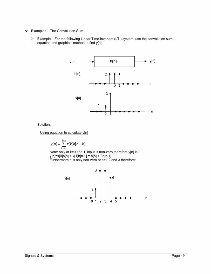
Example – For the following Linear Time Invariant (LTI) system, use the convolution sum
equation and graphical method to find y[n]:
Solution: Using equation to calculate y[n]
][][][ knhkxnyk
k
Note: only at k=0 and 1, input is non-zero therefore y[n] is: y[n]=x[0]h[n] + x[1]h[n-1] = h[n] + 3h[n-1] Furthermore h is only non-zero at n=1,2 and 3 therefore:
n
y[n]
0 1 2 3 4 5
8
2
6
n
h[n]
n
x[n]
1 2 3
0 1
2
1
3
h[n] y[n] x[n]

Signals & Systems Page 50
Using Graphical application of the Convolution Sum to calculate y[n]
h[-k] ”reflected h[k]”
y[n] ”sum of the products of h[n-k] and x[k]”
k -3 -2 -1
2
k
x[k]
0 1
1
3
h[n-k] ”move h[n-k] as n goes from -∞ to +∞”
k n-3 n-2 n-1
2
n -∞ to +∞
n=1 Overlap Region n=4
n 0 1 2 3 4 5
8
2
6

Signals & Systems Page 51
Example - Find the value of y[n] by applying the convolution sum graphically to the following LTI system:
x[n] = otherwise
n
0
401 & h[n]=
otherwise
nan
0
60
Solution:
Apply ][][][ knhkxnyk
k
graphically
K 0
K
K 0
K
0
0
K 0
K
n 0
0
x[k]
h[n-k] for n<0 no overlap
0][][][0
knhkxnyk
h[n-k] for 40 n partial right Overlap
40][][][0
kknhkxnyn
k
Y[n] = 0 for n < 0
= 401
1 1
0
nfora
aa
nn
k
kn
= 641
146
4
nfora
aaa
nn
k
kn
= 1061
744
6
nfora
aaa
n
nk
kn
= 0 for n > 10
n-6 n
h[n-k] for 64 n full Overlap
40][][][4
0
kknhkxnyk
h[n-k] for 106 n partial left Overlap
4)6(][][][4
)6(
knknhkxnynk
h[n-k] for 10n no Overlap 0][ ny
Interval 1:
Interval 5:
Interval 4:
Interval 3:
Interval 2:
4 6 10
y[n]:

Signals & Systems Page 52
Example – Convolution Find the value of y[n] by applying the convolution sum to the following LTI system and input:
Solution: Student Exercise
Example – Find and plot y[n] for an LTI system where: Input, x[n] = 20 sin(0.005πn)u[n-3]-u[n-9] Impulse response, h[n]= 10e-n∂[n+1] + 3∂[n+10] Solution: Student Exercise
h[n] =
]2[][3 nnn
y[n] x[n] =
]6[2]2[]5[3 nununue n

Signals & Systems Page 53
2.3. Sidebar Notes (Useful Relationships)
Geometric Series are useful in simplifying the results of the Convolution Sum: 1) Finite Geometric Series:
r
rrr
nmn
mk
k
1
1
2) Infinite Geometric Series (n=∞) when |r|<1:
r
rr
m
mk
k
1
3) Infinite Geometric Series (n=∞) when |r|<1 and m=0:
r
rk
k
1
1
0
The Geometric Series may be used to derive more complex series such as:
)cos(21
)sin()sin(2
0 xrr
xr
r
kx
kk

Signals & Systems Page 54
2.4. Convolution Integral in Continuous-Time LTI Systems
The convolution integral approach to calculating output in Continuous-Time LTI system is similar to the one introduced in the previous section for the Discrete-Time. Of course the main difference is that the interval between two adjacent points on the signal is infinitely small (∆t0). LTI systems may be characterized by their unit impulse response or simply impulse response, h(t). Impulse response is the superposition of responses of the LTI system to impulse function from negative infinity to positive infinity. The following diagram shows the relationship amongst impulse response, input and output:
Similar to the Discrete-Time, unit impulse function’s sifting property “x()(t-)= x(t)(t-)” can be used to represent a single value of the signal (sample) as shown below:
Extending the sifting property of impulse function, all of input signal, x(t), to the LTI system is represented
x(t)
t
(t-)
t
1
Sifting Property: x()(t-)= x(t)(t-)
t
x()
h(t) Impulse Response y(t)=h(t) dttx )()(

Signals & Systems Page 55
by:
The Continuous-Time convolution integral is a method of finding system output, y(t), that is generated in response to an input signal x(t), using the impulse response function, h(t). It is important to note that x(t) is not necessarily just an impulse function, (t). Conceptually, each non-zero value of input should be multiplied by each non-zero value of h[n] and summed to calculate the value of output. This is implemented by the following equation which is called the convolution integral:
)(*)()(
)()()(
thtxty
dthxty
“The Convolution Integral and corresponding notation”
Another useful tool for understanding and applying the convulsion integral is using graphical approach. The following steps can be used to graphically calculate the output using the convolution integral:
(1) Draw the impulse response transformation, h(t-) * Reflect h()about the k=0 axis which results in h(-) * Shift h(t-)from - to + by changing n from - to +. Identify intervals where h(t-)& x() hold their function and neither is zero.
(2) Calculate the product of x() and h(t-) from - to + Note: There may be many intervals that the products are zero.
(3) Sum the product of h(t-) and x()
h(t) Impulse Response y(t) dtxtx )()()(

Signals & Systems Page 56
Example – The Convolution Integral
Example - Find y(t) for the Linear Time Invariant (LTI) system described by “h(t) = 2u(t)” when
input is “x(t) = e-3t u(t)”. Solution:
h()
x()
1
2
0
0
h(t-)
2
0 t
h(t-)
2
0 t
Interval 1: For t<0 y(t)=0
Interval 2: For t≥0
)1(3
2)(
)(3
22)(
)()()(
3
03
0
3
0
t
tt
t
ety
eedety
dthxty
t -∞ to +∞

Signals & Systems Page 57
Example - Find y(t) for the Linear Time Invariant (LTI) system described by:
Solution
Student Exercise - Find the value of y(t) by applying Convolution Sum to the following LTI system and input:
h(t) =
]2[]1[2 ttt
y[n] x(t)=
)6(2)2()5(4 tututue t
h()
x()
1
1
5
0
h(t-)
1
0 t- 5
h(t-)
1
0
Interval 1: For (t- 5)0 t5
)5(95
95
9
1)()()(
ttt
ededthxty
Interval 2: For t -5 >0 t>5
9
1)()()(
09
0
dedthxty
t- 5
h(t) = u(t-5) y(t) x(t) = e9t u(-t)

Signals & Systems Page 58
2.5. Linear Time-Invariant (LTI) Systems Properties
This section re-examines the system properties which were initially introduced in the previous section. In this section, the focus is on Linear Time-Invariant Systems and the convolution operations. The remainder of this section characterizes LTI systems in-terms of system’s Impulse response, h(t): The Commutative Property
The Commutative Property asserts that the order of convolution does not impact the results. The commutative property is represented by the following equations:
kk
knxnhknhkxnxnhnhnx
dtxhdthxtxththtx
)(][)(][][*][][*][
)()()()()(*)()(*)(
The Commutative property may be proved by replacing “” with “t-p” in continuous-time or replacing “k” with “n-r” in discrete-time.
The Distributive Property The convolution may be distributed over addition without affecting the results. The Distributive Property can be defined by:
][*][][*][])[][(*][
)(*)()(*)()]()([*)(
2121
2121
nhnxnhnxnhnhnx
thtxthtxththtx
The Commutative property may be proved by writing out the convolution sum/integral and factoring out the terms. The implication of Commutative property is that both of the following configurations are equivalent:
The Associative Property The Associative property states that the order of convolution does not affect the result. Below is the restatement of this property in the equation form: .
][*][*][])[*][(*][
)(*)(*)()](*)([*)(
2121
2121
nhnhnxnhnhnx
ththtxththtx
The Associative property may be proved by writing out the sum/integral and factoring out the terms. The implication of Associative property is that all of the following configurations are equivalent:
h1[n]
h2[n]
y[n] x[n]
h1[n]+ h2[n] x[n] y[n]
+

Signals & Systems Page 59
Of course, the same is true for Discrete-Time LTI system.
LTI System with and without memory Memory-less LTI system’s output only depend on the value of present input. Therefore, memory-less system impulse response, h(t) or h[n], satisfies the following relationships: h[n]=0 for n0 h[n]=K[n] y[n]=Kx[n] “Discrete-Time” h(t)=0 for t0 h(t)=K(t) y(t)=Kx(t) “Continuous-Time” All other systems are LTI systems with memory, by definition.
Invertibility of LTI Systems A system is invertible only if an inverse system and impulse response exist that when connected in series to the original system, produces an output equal to the input of the first system.
In order for the Invertibility to be true, h1(t) * h2(t) must be an identity function, (t) where h1(t) is the original system impulse response and h2(t) is the inverse system impulse response. The following equation restates the definition of invertible system: h1(t) * h2(t) = (t) h1[n] * h2[n] = [n] Example -- A system’s input and output are related by the following equation:
y(t)=5x(t- 4) Is this system invertible? Solution: We need the system impulse response in order to answer the question of Invertibility. By inspecting the given input/output relationship, it is clear that the output is equal to the input shifted and scaled. Therefore: h1(t) = (1/5) (t - 4) “System Impulse Response”
Identity System, (t) x[n] x[n]
h1[n] h2[n] x[n] x[n] y[n]
h1(t) h2(t) y(t) x(t)
h2(t) h1(t) x(t) y(t)
h2(t) * h1(t) x(t) y(t)
h1(t) * h2(t) x(t) y(t)

Signals & Systems Page 60
System is invertible only If an inverse impulse response, h2(t), can be find such that h1(t)*h2(t) = (t). It can be seen that h1(t) = 5 (t + 4) would satisfy the Invertibility requirement: h1(t)* h2(t)= (1/5) (t- 4)* (5)(t + 4)= (t)
Student Exercise – Show that LTI system with impulse response h1[n]=u[-n+2] is invertible by calculate the inverse impulse response and testing it. Hint: u[n]*( [n] - [n-1]) = [n]
Causality of LTI Systems In a causal LTI system, the system’s present output only depends on the present and past input. In other words, the system is non-causal if the system output depends on the future input. For a causal Discrete-Time LTI system, y[n] does not depend on x[k] where k > n. This requirement translates to the rule that in a causal system, h[n]=0 for n<0.
Examine the Convolution sum
k
knxkhny ][][][ , to relate the two requirements.
Similar requirements for causality exists in continuous-time which states that h(t)=0 for t<0 in causal systems. In summary, a system is causal if its impulse response “h(t) or hn]” is zero for “t<0 or n<0”.
Stability for LTI Systems A system is stable if for every bounded input, the out is also bounded. Below is a restatement of stability definition in-term of impulse response: Discrete-Time
Input is bounded |x[n]| < A for all n where A is a finite value
|][|||][||][][||][|
kk
khAnyknxkhny for all n
The above equation is true if:
|][|k
kh then the system is stable
Continuous-Time
Using a similar process to Discrete-Time, we can conclude that if:
dh |][| then the system is stable
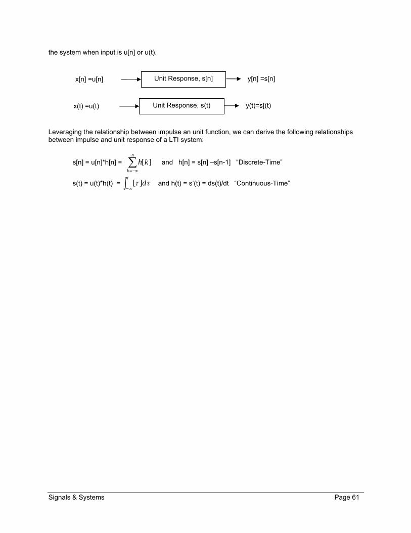
Although impulse response is used commonly to characterize systems, LTI systems may also be characterized by the unit step response, s[n] or s(t). The unit step response, s[n] or s(t), is the output of
Signals & Systems Page 61
the system when input is u[n] or u(t).
Leveraging the relationship between impulse an unit function, we can derive the following relationships between impulse and unit response of a LTI system:
s[n] = u[n]*h[n] =
n
k
kh ][ and h[n] = s[n] –s[n-1] “Discrete-Time”
s(t) = u(t)*h(t) =
td ][ and h(t) = s’(t) = ds(t)/dt “Continuous-Time”
Unit Response, s[n] x[n] =u[n] y[n] =s[n]
Unit Response, s(t) x(t) =u(t) y(t)=s[(t)

Signals & Systems Page 62
2.6. Differential/Difference Equations
Differential/Difference equations can be used to describe important subclasses of LTI systems. The linear constant-coefficient differential equation is used for continuous-time and the linear constant coefficient difference equation is used for discrete-time. Although these subclasses are more limited in scope, they serve as tools in analysis of an important subclass of systems such as the RC and RL circuits. Additionally, they serve as the basis for study of broader types of signals and systems. This section introduces and applies difference and differential equations with linear constant-coefficient. Linear Constant-Coefficient Differential Equations
First, let’s use an RC circuit to derive linear constant-coefficient differential equation. In the following LTI system, voltage is the input, x(t), and current is the system output, y(t)::
.Using KVL )()(
1.0)(200 txdt
tdyty
One difference is that in this equation y(t) is not given in-term of x(t). We must solve the differential equation to find the output. The solution will have constants which would require additional relationships between input/output such as initial condition in order to find the constants’ value. Solution to an ordinary linear differential equation may be written as: y(t) = yp(t) + yh(t) where yp(t) or the particular solution will be the same form as the input in this case yp(t)=Ae2t yh(t) or the homogenous solution will have the form yh(t)=Best with x(t)=0 Talking advantage of superposition property of the LTI system, we can find each portion of the solution (output or response) and then sum them to find the total solution. First, plug yp(t)=Ae2t (same as input except for the coefficient) into the differential equation to find the Particular solution:
t
p
tt
t
etyAAA
edt
AedAe
2
22
2
02.0)(2.200/442.0200
4
1.0200
Second, plug yh(t)=Best (power or coefficient are unknowns) into the differential equation where x(t)=0 to find the homogenous solution:
t
hst
stst
BetyssBes
equationldifferntiaogeneousfortxdt
BedBe
01.0)(01.00)2.0200(0)2.0200(
"hom0)("0
1.0200
Therefore the total solutions is : y(t)= yp(t)+ yh(t)= 0.02e2t + Be-0.01t Now, we need to find the coefficient B by using the initial state if not given, assume y(t0)=0 with the
+ -
200 Ω
100 mH v=L(di/dt)
x(t)=4e2t
y(t)=i(t)
Signals & Systems Page 63
total solution equation. We will assume at the initial state (t0=0), the system is at rest y(0)=0, therefore:
02.0002.0)0( BBy
Therefore y(t)= yp(t)+ yp(t)= 0.02e2t – 0.02e-0.01t Key take away from this section are:
(1) Total solution consists of particular (with input) solution and homogeneous solutions (input set to 0). Homogeneous solution is considered natural response since x(t)=0.
(2) To find all the constants, equations based on system condition at a given time (t0) are required. It is common to assume that system is at rest at time t=0 therefore y(0)=0.
(3) In the example and description presented in this section, we used first order equations. The same approach may be applied to higher order linear constant-coefficient differential equations such as the one shown by the following general form:
k
kQ
kkj
jP
jj dt
txdb
dt
tyda
)()(
00
Linear Constant-coefficient Difference Equations
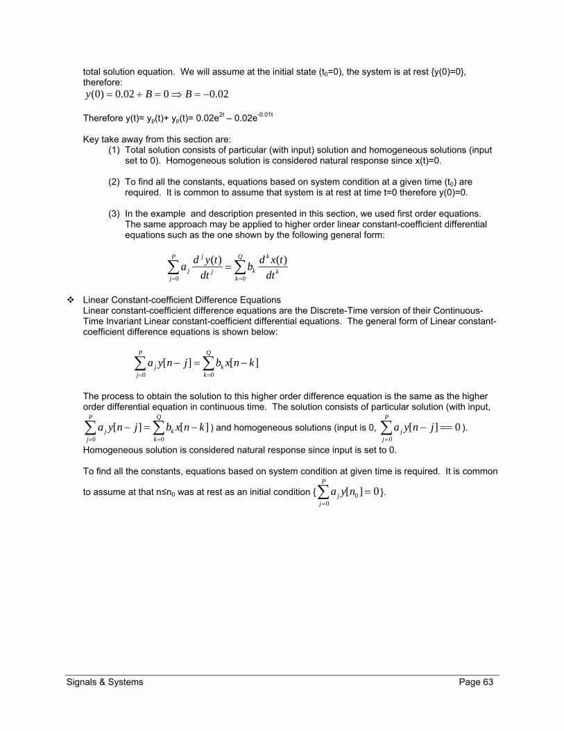
Linear constant-coefficient difference equations are the Discrete-Time version of their Continuous-Time Invariant Linear constant-coefficient differential equations. The general form of Linear constant-coefficient difference equations is shown below:
][][00
knxbjnyaQ
kk
P
jj
The process to obtain the solution to this higher order difference equation is the same as the higher order differential equation in continuous time. The solution consists of particular solution (with input,
][][00
knxbjnyaQ
kk
P
jj
) and homogeneous solutions (input is 0, 0][0
jnyaP
jj ).
Homogeneous solution is considered natural response since input is set to 0. To find all the constants, equations based on system condition at given time is required. It is common
to assume at that n≤n0 was at rest as an initial condition 0][ 00
nyaP
jj .

Signals & Systems Page 64
Graphical representation of the difference and differential equations One advantage of these equations is that they can be intuitively and easily described by graphical representation. Here are some of the common symbols used in the graphical representations:
For example the differential equation )()(
1.0)(200 txdt
tdyty may be rewritten as:
)(005.0)(
0005.0)( txdt
tdyty and can be represented graphically as shown below:
The same system may also be represented using integrators by rewriting it as
tdyxty )](2000)(10[)( and presented graphically as:
y(t)
-2000
+ x(t) 10
y(t)
-0.0005
D
+ x(t) 0.005
+ x1
x2
x1+x2
Adder Scalar
kx x k
D
Unit Delay or Differentiator
x[n] x[n-1]
D x(t) dx(t)/dt
Integrator
x(t)
tdx )(

Signals & Systems Page 65
2.7. Chapter Summary
This section is a summary of key concepts from this chapter. Discrete-Time Convolution Sum
][*][][
][][][
nhnxny
knhkxnyk
k
Continuous-Time Convolution Integral
)(*)()(
)()()(
thtxty
dthxty
Linear Time-Invariant (LTI) System Properties Associativity Causality Commutativity Distributivity Invertibility Linearity Memory Stability

Signals & Systems Page 66
2.8. Additional Resources
Oppenheim, A. Signals & Systems (1997) Prentice Hall
Chapter 2
Modern Digital & Analog Communication Systems (1998) Oxford University Press Chapter 2
Stremler, F. Introduction to Communication Systems (1990) Addison-Wesley Publishing Company Chapt 2
Birkhoff, G. Ordinary differential equations (1978) J. Wiley and sons

Signals & Systems Page 67
2.9. Problems
Refer to www.EngrCS.com or online course page for complete solved and unsolved problem set.

Signals & Systems Page 68
Chapter 3. Fourier Series Representation of Periodic Signals
Key Concepts and Overview Overview & History of Fourier Series
Complex Exponential Signals and LTI System Responses
Fourier Series Representation of Continuous-Time Periodic Signals
Convergence of the Continuous-Time Fourier Series
Continuous-Time Fourier Series Properties
Fourier Series Representation of Discrete-Time Periodic Signals
Discrete-Time Fourier Series Properties
Application of Fourier Series in LTI systems
Filtering in Continuous-time and Discrete-Time
Additional Resources

Signals & Systems Page 69
3.1. Overview & History of Fourier series
This chapter introduces Fourier series in the context of Linear Time Invariant (LTI) Systems when input signal is periodic. The concepts will be developed both in Continuous-Time and Discrete-time. As discussed earlier, all periodic signals can be represented using complex exponential form. Additionally, it will be shown that most periodic signals may be represented as a Fourier series which is a weighted sum of harmonics (integer multiples) of the fundamental frequency. Fourier series and LTI system properties lead to relationship between input and output which are useful in finding the LTI system response to periodic signals. In future chapters, the concepts developed here will be broaden to include aperiodic (Not periodic) signals. Form a historical point-of-view, the work started with Euler in 1748 but Fourier made the key observation that period signals can be represented as a trigonometric series in 1802 and he also understood that this is a very important class of signals. Fourier’s findings are viewed as the core concept which is the reason for the series being named for Fourier. Dirichlet in 1829 developed the precise mathematical representation, now known as Fourier series. But it was not until 1965, when Cooley and Tukey discover a method called Fast Fourier Transform (FFT) which enable engineers to design computer programs that would perform functions such as filtering fast enough to make it useful. FFT along with the advent of higher performance computer has led to use for Fourier transforms and series is design majority of signal processing devices. In a nutshell, Fourier series allows us to represent any signal as a series of harmonic signal components. So to filter any frequency, simply zero the coefficient for the corresponding harmonic. In general, we can reshape any signal by simply changing the coefficient of its harmonic components. Although in this text, our interest in Fourier series is in its application to audio, video, electrical and computing fields, the Fourier series concept has much wider use including heat transfer and mechanical systems.

Signals & Systems Page 70
3.2. Complex Exponential Signals and LTI System Responses
As discussed earlier, Complex Exponential signals can be used to represent any periodic signal. Since we are focusing on LTI systems then the response to a periodic signal will be a linear combination of the complex exponential terms. Let’s start by defining a few terms to use in our development of Fourier series for complex exponential signals and LTI systems. The following table defines input and Responses:
Input Response Continuous-time est H(s)est Discrete-time zn H(z)zn Where:
s and z are complex numbers but for the purposes here we can define them as:
(1) s = jw “pure imaginary” (2) z=ejw
H(s) and H(z) are complex functions of s and z accordingly Response may or may not be complex Input est or zn are referred to as the eigen function H(s) for a specific value of sk is referred to as the eigen value associated with
eigen function sk. This is the value that is multiplied by eigen function to find the response.
Using the above definition for input, our next step is to find eigen values H(s) and H(z) in terms of the system impulse response h(t) and h[n] for continuous-time and discrete-time respectively. Determining the value of H(s) in terms of h(t) for a continuous-time LTI System
Here is a graphical restatement of the LTI system with Impulse response h(t) and a periodic input signal x(t) and response y(t).
In order to find the eigen value H(s), we need to apply the convolution definition to find the response to this system:
dehsHWhereesHty
dehedehdtxhtxthty
sst
sstts
)()()()(
)()()()()(*)()( )(
Notes: ejwt is referred to as the eigen function (input) H(s) for a specific value of sk is referred to as the eigen value associated with eigen function
sk. System Response is equal to eigen function multiplied by eigen function.
Determining the value of H(z) in terms of h[n] for a discrete-time LTI System Following a similar process as the Continuous-Time, H(z) can be determined in term of h[n].
LTI system h(t)
x(t)=est y(t)=H(s)est

Signals & Systems Page 71
k
kn
k
kn
k
kn
k
zkhzHWherezzHny
zkhzzkhknxkhnxnhny
][)()(][
][][][][][*][][ )(
Notes: zn or ejwn is referred to as the eigen function (input) H(s) for a specific value of zk is referred to as the eigen value associated with eigen function
zk. System Response is equal to eigen function multiplied by eigen function.
Response to Generalized Input Generalized input signal may have many terms (eigen functions) which leads to system response being sum of responses to each eigen function and will have associated eigen value. Starting with the Continuous time LTI system, Let’s use the multi-term input
tststs eaeaeatx 321321)(
Applying the eigen function property, the response (output) to each input terms can be written as follows:
tsts
tsts
tsts
esHaea
esHaea
esHaea
33
22
11
)(
)(
)(
333
222
111
Now, we can apply the superposition since the system is linear which means response to the sum of inputs is the sum of individual responses:
tststs esHaesHaesHaty 321 )()()()( 332211
We can generalize the above derivation for LTI systems as:
k
tskk
k
tsk
kk esHatyeatx )()()(
Similar process can be used to derive the generalized response for Discrete-time LTI system which is shown below:
k
nkkk
k
nkk zzHatyzanx )()(][
Examples - eigen value and eigen function
LTI system h[n]
X[n]=zn Y[n]=H(z)zn

Signals & Systems Page 72
Example 1: In a LTI System, output is related to input by a time shift of -4 find eigen value associate with eigen function x(t) = ej2t Solutions y(t) = x(t+4) = ej2(t+4) = ej8 ej2t So we can say that eigen function is ej2t =est= ejwt which means s=2j or w=2. Also eigen value H(s)= e4s for s=j2 is H(s=j2) = ej8
Note: h(t) = δ(t-4), so we can use the convolution to confirm the output.
Example 2: Given the eigen value H(s) = e-2s find the response to the input (eigen function) x(t) = cos5t Solutions: x(t) = cos(5t) = cos(wt) w=5 rad/s s=j5 y(t) = H(s)x(t) = e-2scos(5t) = e-j10cos(5t) Applying Euler’s Identify cos(a) = ½ (eja + e-ja) y(t)= ½ (ej(5(t-2) + e-j(5(t+2)) Applying Euler’s identify again y(t) =cos(5(t-2)) So input is shifted in time by 2 when the eigen value is H(s) = e-2s
Example 3: Given the eigen value H(s) = e-2s, find the response to the input x(t) = cos(5t) + sin(9t). Note: Find eigen value for each component. Solutions: ”Student Exercise”
Example 3: Find eigen value, H(s), for the following Circuit:
Solutions: ”Student Exercise”
-
+
+ x(t)
-+
y(t) -
R
C

Signals & Systems Page 73

Signals & Systems Page 74
3.3. Fourier Series Representation of Continuous-Time Periodic Signals
As mentioned earlier, Fourier Series is a representation of Continuous-Time periodic signals in terms of weighted sum of signal’s harmonics. The first step in the Fourier Series development process is to define the Periodic signal. A signal is periodic, if for some positive value of Period, T, the following equality holds: x(t) = x(t+T) for all t. Fundamental period of x(t) is the minimum, positive, nonzero value of T that satisfies the above equation. Further, W0 = 2/T is referred to as fundamental frequency. Harmonically related periodic signal representations with fundamental frequency w0 simply uses signals with frequencies that are integer multiples of w0. This means that the harmonic signals have period Tk which is a fraction of the fundamental Period T= 2/w0. Below are some examples of harmonically related signals:
Sinusoidal Signal, x1(t) = cos (w0t) The harmonically related signals of x1(t) can be represented as:
...,2,1,0/T)t)2cos(k( t)cos(k (t) 0k kwherew
Pure Imaginary Exponential Signal, tjw2
0e (t)x
The harmonically related signals of x2(t) can be represented as:
...,2,1,0e e (t) /T)tjk(2tjkk
0 kwherew
The following facts are important to consider when working with the harmonically related periodic signal representations:
(1) Each of the harmonics has a frequency which is multiples of fundamental frequency. (2) Signal component with k=0 is constant (3) Signal component with k=+1 and -1 is referred to as the first harmonics or fundamental (4) Signal component with k=+2 and -2 is referred to as the second harmonics (5) Signal component with k=+N and -N is referred to as the Nth harmonics
The linear combination of harmonically related signals is also periodic which means that the following general form of harmonically related signals is periodic:
k
tTjkk
k
tjkwk eaeatx )/2(0)(
Fourier Series Representation
This representation of Periodic signal is referred to as the “Fourier Series Representation” where ak is referred to as the Fourier Coefficient. Examples - Fourier Series Representation
Example 1: Plot a periodic signal x(t), with fundamental frequency w0= with the following Fourier
series Coefficients: a0 = 1; a1=a-1=1/3; a2=a-2=1/2; all other coefficients are 0 Solutions

Signals & Systems Page 75
First write out the Fourier Series
)(2
1)(
3
11)(
2
1
3
11
3
1
2
1)(
22
202
0
0
tjtjtjtj
k
tjkwk
tjtjtjtj
k
tjkwk
eeeeeatx
eeeeeeatx
Apply Euler’s Identity (eja + e-ja) = 2cos(a) x(t) = 1 + 2/3 cos(t) + cos(2t)

Signals & Systems Page 76
x0(t)=1
t
x1(t)= 2/3 cos(t)
t
x2(t)= cos(2t)
t
x(t)= x0(t) + x1(t) + x2(t)= 1 + 2/3cos(t) +cos(2t)
t 0
3

Signals & Systems Page 77
Example - Plot a periodic signal x(t), with fundamental frequency w0=/2 with the following
Fourier series Coefficients: a0=1; a1=a-1=2; a2=a-2=3; a3=a-3=1/5; all other coefficients are 0 Verify your results using Matlab. Solutions ”Student Exercise”
Example – Draw time domain and frequency domain, and find values of non-zero Fourier series coefficients (ak) for the following signals: a) A DC signal with magnitude of 2. b) x(t) = ej50πt c) x(t) = sin(200πt) Solutions ”Student Exercise”

Signals & Systems Page 78
Alternative Forms of Fourier Series Representations There are three forms of Fourier Series Representation which are commonly used. All these forms are mathematically equivalent:
k
tjkwk eatx 0)( “This is the form that is most commonly use in this text”
kjkk
kkk eAawheretkwAatx
1
00 )cos(2)(
kkkk
kk jCBawheretkwjCtkwBatx
1000 )sin()cos(2)(
It is highly recommended that students proof that all three are mathematically equivalent.
Calculation of the Fourier Series Representation of a Continuous-time Periodic Signal In order to derive the Fourier Series Representation, we need to have the original signal’s fundamental frequency and Fourier Series Coefficient ak. The fundamental frequency can be obtained from the signal. Below is the process for finding the Fourier Series Coefficient, ak. We know that any periodic signal can be represented by the following Fourier Series Representation:
k
tjkwk eatx 0)( Fourier Series Synthesis Equation
Our objective here is to find the Fourier Coefficients, ak for a given signal x(t). We will start by multiplying both side of the Fourier Series Synthesis Equation by e-jnwot.
k
tjnwtjkwk
tjnw eeatxe 000 )(
Next, integrate both side over one fundamental period (from 0 to T=2/w0)
k
Ttwnkj
k
Ttjnw
T
k
tjnwtjkwk
Ttjnw
dteadttxe
dteeadttxe
0
)(
0
00
00
000
)(
)(

Signals & Systems Page 79
Side Bar We can simplify the integral inside the bracket as shown below using the Euler’s identity:
TTT
twnkj dttwnkjdttwnkdte0
0
0
0
0
)( )sin()cos(0
When (k-n)= 0 or k=n then TTT
twnkj Tdtjdtdte000
)( 00
When (k-n)≠ 0 or k≠n then
000
sincos0
)( 0
periodoneforareaeperiodoneforareainedteT
twnkj
Therefore
kk
Ttwnkj
k Tadtea0
)( 0
Using the derivation of the side bar, we can rewrite the above equation as:
Tadttxe k
Ttjnw
0
)(0
Which can be re-arrange to find the Fourier Coefficient an
T
tjkwk
Ttjkw
k dttxeT
aordttxeT
a )(1
)(1
00
0
Fourier Series Analysis Equation
Summary of Fourier Series equations for a periodic continuous-time signal
k
tTjkk
k
tjkwk eaeatx )/2(0)( Synthesis Equation
T
tTjk
T
tjkwk dttxe
Tdttxe
Ta )(
1)(
1 )/2(0 Analysis Equation
* ak is referred to as the Fourier Series Coefficient or the spectral coefficients of x(t) Note of interest: Euler and Lagrange both knew this equation in 18th century but they did not see it as important since they did not feel it cover large enough class of periodic signal. Fourier a hundred years later showed that they indeed cover a large class which is the reason these equations are named for Fourier.
Example - Fourier Series Application Example - What are the Fourier Series Coefficients of x(t)=sin(wot)?
Solutions
You can use the analysis equations to find the coefficient TwdttxeT
a o
T
tjkwk /2,)(
10
But the easier way would be to use Euler’s identity )(2
1sin jaja ee
ja

Signals & Systems Page 80
so tjwtjwo
oo ej
ej
twtx 2
1
2
1sin)(
a1 = 1/2j , a-1 = -1/2j , ak = 0 for k≠-1 & k≠+1 Below is the bar graph of the Fourier Series Coefficient:
Example: What is the Fourier Series Coefficient for the period Square Wave where:
T
tTjk
T
tjkwk dttxe
Tdttxe
Ta )(
1)(
1 )/2(0
“Fourier Series Coefficient can be calculated over any period”, for this problem period from –T/2 to T/2 is one of the easiest.
1
1
01
T
T
tjkwk dte
Ta
for k=0 T
Tdt
Ta
T
T
o121 1
1
for k≠0 k
Tkw
Tkw
Tkw
j
ee
Tkwdte
Ta o
o
oTjkwTjkw
o
T
T
tjkwk
)sin()sin(2
2
21 1110101
1
0
Note: above simplification uses Euler’s identity )(2
1sin jaja ee
ja & wo = 2/T
x(t)
1
-T T -T1 T1 T/2 -T/2
. . . . . .
x(t) = 1 for |t| < T1 0 for T1 < |t| < T/2
Coefficient Magnitude
-1 0 1
Coefficient Phase
k
1/2
-1 0 1k
+90o
-90o
1/2
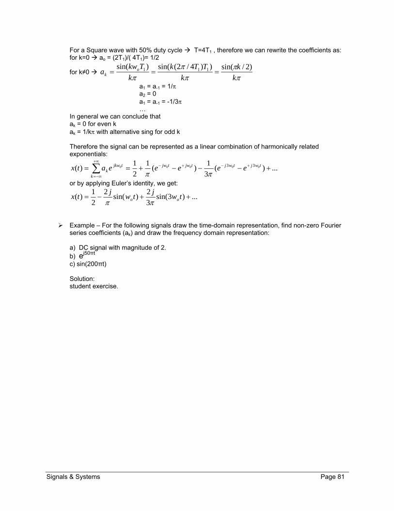
Signals & Systems Page 81
For a Square wave with 50% duty cycle T=4T1 , therefore we can rewrite the coefficients as: for k=0 ao = (2T1)/( 4T1)= 1/2
for k≠0
k
k
k
TTk
k
Tkwa o
k
)2/sin())4/2(sin()sin( 111
a1 = a-1 = 1/ a2 = 0 a1 = a-1 = -1/3 … In general we can conclude that ak = 0 for even k ak = 1/k with alternative sing for odd k Therefore the signal can be represented as a linear combination of harmonically related exponentials:
...)(3
1)(
1
2
1)( 00000 33
twjtwjtjwtjw
k
tjkwk eeeeeatx
or by applying Euler’s identity, we get:
...)3sin(3
2)sin(
2
2
1)( tw
jtw
jtx oo
Example – For the following signals draw the time-domain representation, find non-zero Fourier series coefficients (ak) and draw the frequency domain representation: a) DC signal with magnitude of 2. b) ej50πt c) sin(200πt) Solution: student exercise.

Signals & Systems Page 82
3.4. Convergence of the Continuous-Time Fourier Series
Fourier Series can represent an extremely large class of periodic signals including square wave as shown earlier. The full representation is a linear combination of an infinite number of harmonically related complex exponentials. The immediate question is how many terms are sufficient in representing the signal accurately. From the previous section, we know that x(t) is fully described by the following:
k
tjkwk eatx 0)(
In a finite sum, the positive and negative infinity limits needs to be replaced by a finite value of (-N to N) which means xN(t) value is a Nth approximation of x(t) and is written as:
N
Nk
tjkwkN eatx 0)( Nth approximation of x(t)
To answer the question of when finite sum is a good enough approximation, we need calculate the approximation error as shown below:
N
Nk
tjkwkNN eatxtxtxte 0)()()()( Approximation Error
The goodness of approximation is quantitatively measured by the energy of the error in one period as shown below:
T
N dtperiodainerrorofPowerE Energy of Error over one period =
or
T
NN dtteE 2|)(|
An approximation with EN equal to zero means that the original and approximated signal have the same energy so it is a good approximation to the original signal. It is important to realize that it does necessarily mean that the approximated signal is the same as the original signal x(t). A signal has a Fourier Series representation if and only if: as N ∞ , eN(t) 0 and xN(t) x(t)
This type signal are said to converge which means as k goes to infinity, T
tjkwk dttxe
Ta )(
10 and
k
tjkwk eatx 0)( converge.
The good news is that there are large classes of signals that have no convergence problem. And for these signals Fourier Series representation exists. Even though a Fourier Series representation exists for convergent signals, it does not mean that the Fourier Series representation and original signal have the same value at every point. For example in the case of signals with discontinuities such as a square wave, at the discontinuities the Fourier Series Representation takes on the average value of signal from the two sides of the discontinuity.

Signals & Systems Page 83
Convergence Conditions and Dirichlet’s three Conditions Again, a signal does not converge if:
(1) T
tjkwk dttxe
Ta )(
10 does not converge (meaning ak goes to ∞)
or
(2) At times ak converge but the sum
k
tjkwk eatx 0)( does not converge
(meaning x(t) goes to ∞)
Criteria for deciding if a signal has a (Converging or valid) Fourier Series Representation The periods that have finite energy over a single period will have Fourier Series Representation. Dirichlet developed three conditions that when met, it is given x(t) equals its Fourier Series representation excluding for values of t that x(t) is discontinuous. Condition 1
Over any one period, x(t) Must be absolutely integrable; meaning T
dttx |)(|
For example the following x(t)t fails condition 1:
Other signals that fail this condition include e1/sin(t) and tan(1/sin(t)).
Condition 2 In any finite interval of time, x(t) is has finite variation; meaning there is no more than a finite number of maximum of minimum during a single period. For example the following x(t)t fails condition 2:
t
x(t)
-2a -a 0 a 2a

Signals & Systems Page 84
sin(1/sin(t)) is example of a signal that fail this condition.
Condition 3 In any finite interval of time, there are only a finite number of discontinuities. Each discontinuity also must be finite.
As you can see signal that do not meet the Dirichlet’s three conditions are not common. It is safe to say that most natural signals are convergent and have a Fourier Series Representation.
Observations Relating to Signal Discontinuity For a periodic signal that has no discontinuity, the Fourier Series Representation converges and equals the original signal at every value of t as N∞ where N is number of terms used in approximation. For a periodic signal with a finite number discontinuities in each period, the following holds true:
the Fourier Series Representation equals the signal everywhere except at the isolate points of discontinuity at which the series converges to the average value of signal on each side of the discontinuity.
Gibbs phenomenon is also present, meaning as the finite N (number of terms) increases, the peak amplitude of the error move toward the discontinuities but the error peak values remain constant.
t
x(t)
-2a -a 0 a 2a
… … … ……
t
x(t)
-2a -a 0 a 2a
… … … … …

Signals & Systems Page 85
The following diagram demonstrated the two stated properties for a square wave as the number of terms to approximate the signal, N, is increased: (N=1, 5, 17)
t
xN(t) with N=1
-T 0 T
a/2
a
t -T 0 T
a/2
a
xN(t) with N=5
t -T 0 T
a/2
a
xN(t) with N=17

Signals & Systems Page 86
3.5. Continuous-Time Fourier Series Properties
In this section we will cover some of the properties of Fourier Series which are used in future exercises and analysis of signal and systems. These properties not only provide us with insights, they also are crucial is reducing complexity. The following notation to show that ak is the Fourier series coefficient of signal x(t):
kFS atx )(
The proofs for the properties presented in this section are left to the reader. The proofs consist of plugging in the values into the synthesis or analysis equations in order to show that equality holds. The remainder of this section is dedicated to Fourier Series Properties: Linearity
Let x(t) and y(t) denote two periodic signals with period T and fundamental frequency wo = 2/T. x(t) and y(t) have Fourier Series coefficient ak and bk respectively:
k
FS
kFS
bty
atx
)(
)(
Linearity property states that:
kkkFS BbAactBytAxtz )()()(
ck is Fourier coefficient of z(t) where A and B are constants.
Time Shifting When a time shift is applied to a periodic signal x(t), the period T, fundamental frequency wo = 2/T and magnitude of the signal is preserved. Time Shifting property states that:
k
tjkwFS
kFS
aettx
atxoo
)(
)(
0
Time Reversal
When a time reversal is applied to a periodic signal x(t), the period T, fundamental frequency wo = 2/T and magnitude of the signal is preserved. Time Reversal property states that:
k
FS
kFS
atx
atx
)(
)(
Two note of interest relating to time reversal:
If x(t) is even, meaning x(t)=x(-t) ak = a-k if x(t) is odd , meaning x(t) = -x(-t) ak = - a-k
These two observations can be used to determine if a function is odd or even based on their Fourier
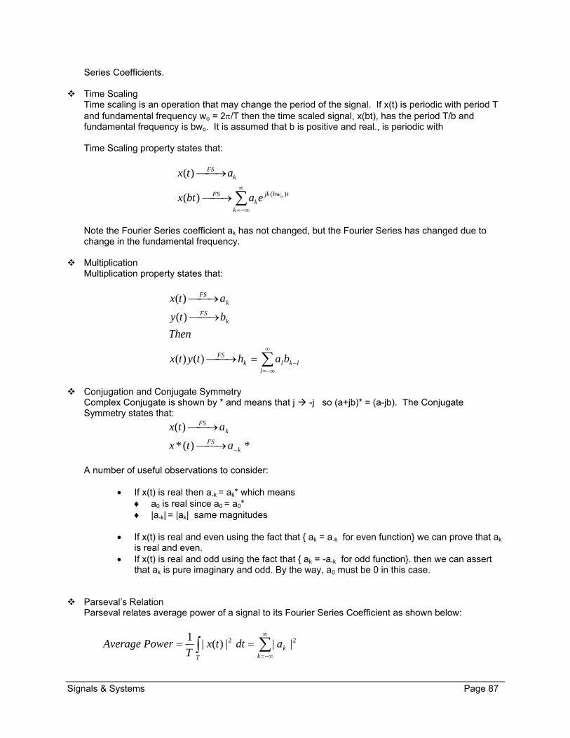
Signals & Systems Page 87
Series Coefficients.
Time Scaling Time scaling is an operation that may change the period of the signal. If x(t) is periodic with period T and fundamental frequency wo = 2/T then the time scaled signal, x(bt), has the period T/b and fundamental frequency is bwo. It is assumed that b is positive and real., is periodic with Time Scaling property states that:
k
tbwjkk
FS
kFS
oeabtx
atx
)()(
)(
Note the Fourier Series coefficient ak has not changed, but the Fourier Series has changed due to change in the fundamental frequency.
Multiplication Multiplication property states that:
llklk
FS
kFS
kFS
bahtytx
Then
bty
atx
)()(
)(
)(
Conjugation and Conjugate Symmetry
Complex Conjugate is shown by * and means that j -j so (a+jb)* = (a-jb). The Conjugate Symmetry states that:
*)(*
)(
kFS
kFS
atx
atx
A number of useful observations to consider:
If x(t) is real then a-k = ak* which means a0 is real since a0 = a0* |a-k| = |ak| same magnitudes
If x(t) is real and even using the fact that ak = a-k for even function we can prove that ak
is real and even. If x(t) is real and odd using the fact that ak = -a-k for odd function. then we can assert
that ak is pure imaginary and odd. By the way, a0 must be 0 in this case.
Parseval’s Relation Parseval relates average power of a signal to its Fourier Series Coefficient as shown below:
k
k
T
adttxT
PowerAverage 22 |||)(|1

Signals & Systems Page 88
To prove, replace x(t) with the synthesis equation and simplify the equation. The process is similar to proving the properties.
Properties of continuous-time Fourier Series
Properties
Periodic Signal x(t) and y(t) with w0 = 2/T
Fourier Series Coefficient ak and bk
Conjugate symmetry Real x(t) ak=a-k* Conjugation x*(t) a-k
* Convolution, Periodic dtyx
T
)()( T ak bk
Differentiation
dt
tdx )(
jkw0ak
Frequency Shifting )(txetjQwo ak-Q
Integration
t
dx )( periodic & finite only if a0 =0 ak / jkw0
Linearity Ax(t) + By(t) Aak + Bbk Multiplication x(t)y(t)
llklba
Parseval’s Relation Average Power for Periodic signals
k
k
T
adttxT
PowerAverage 22 |||)(|1
Real and Even Signals Real and even x(t) ak is real and even Real and Odd Signals Real and odd x(t) ak is purely imaginary and odd Time Reversal x(-t) a-k Time Scaling x(bt)
b>0 Period =T/b and w0 = 2b/T ak
Time Shifting x(t-t0) k
tjkw ae oo
Examples – Properties of continuous-time Fourier Series
Example - Use the following properties of x(t) to determine the x(t) function:
1) x(t) is periodic with T=2 2) x(t) has Fourier Series Coefficient ak 3) ak =0 for |k| ≥ 2 4) x(t) is a real signal 5) DC component of the signal is 1/3 6) Magnitude of fundamental frequency component is 1/5. Solution Property 1 w0 = 2/T = Property 2 & 3 all ak=0 except a-1, a0, a1
Property 4 a1 = a-1*
Property 5 a0 = 1/3 Property 6 a1 = 1/5

Signals & Systems Page 89
Using above information and synthesis equation:
tjtjtjkwtjkw
k
tjkwk eeeaaeaeatx )5/1(3/1)5/1()( 000
101
Example – Find x(t+5) given x(t) has the following non-zero Fourier Series Coefficients:
a-1 = 2, a0 = 5+j, a4 = 3. Solution
Example – Given real function x(t) with non-zero Fourier Series Coefficients a-1=a1=3 and a-
2=a2=4, a) Find Fourier Series Coefficients for x(9t). b) What’s fundamental frequency of x(9t). c) What’s the approximation of x(t) using Fourier Series. Solution a) Same as x(t) b) 9w0
c) twjtwjtwjtwj
twjtwjtwjtwj
k
tjkwk
eeee
eeeeeatx
0000
00000
189918
9)2(9)1(9)1(9)2(
4334
4334)9(
Example – Given that function x(t) has the Fourier Series Coefficients a-1 = 2+j , a0 = 5, a+1 = 2-j, determine if x(t) is real and/or even/odd. Solution ak = a-k* x(t) is real It’s neither odd or even.
Example – for a 100 Hz square wave signal with 50% duty cycle, maximum of 5v and minimum of 0v, a) Find the Fourier Series Coefficients b) find N-term approximation of x(t) Solution

Signals & Systems Page 90
3.6. Fourier Series Representation of Discrete-Time Periodic Signals
Development of Fourier Series Representation of Discrete-Time Periodic Signals is similar to the process used for the Continuous-time and the results are similar also. The one key difference is that Discrete-time Fourier Series representation is a finite series as opposed to infinite series representation required for continuous-time periodic signals. This difference means that the Discrete-Time Fourier Series does NOT have convergence issue. Now let’s start the process of finding the relationship between the discrete-time signal and its Fourier Series (Synthesis and Analysis equations) Again, periodic Discrete-time Signal x[n] is a signal that meets the following definition:
x[n]=x[n+N] The Fundamental period is the smallest positive integer N for which x[n]=x[n+N] Fundamental Frequency w0=2/N
Discrete-Time Fourier Series Equations
Any periodic signal can be represented mathematically in complex exponential form. Each term of the complex exponential signal may be represented by:
,...3,2,1][ 00 )/2( keen nwNjknjkwk
Signals represented by these terms have frequencies which are multiple of the fundamental frequency (w0=2/N). These terms represent the signal harmonics. We can restate the definition of Periodic signal in Discrete-time by the fact that all terms of the complex exponential signal with same relative location in the period are equal. The following equation restates this fact:
][][ )( nn rNkk where r is an integer and N is the fundamental Period.
The Discrete-Time Fourier Series is also a linear combination of harmonically related complex exponentials. The proof is similar to the Continuous-Time and starts by writing the convolution sum. The following equation pair are the general Discrete-Time Fourier Series Synthesis and Analysis Equations:
1,...,1,
][ )/2(
Nmmmkfor
eaeanxNk
nNjkk
Nk
njkwk
o
Fourier Series Synthesis Equation
Nn
nNjk
Nn
njkwk enx
Nenx
Na o )/2(][
1][
1 Fourier Series Analysis Equation
Where: 1) x[n] is a periodic signal 2) N is the Fundamental Period 3) m is an arbitrary integer 4) ak is Fourier Series coefficient (ak = ak + N)
Example - Fourier Series Representation of Discrete-Time Periodic Signals

Signals & Systems Page 91
Example1: Find the Fourier Series coefficients For the signal x[n] = sin(w0n). Solution Although we could use the analysis equation to find ak, an easier way would be to use the Euler equation to reshape the signal to its linear exponential format select coefficients so that would be equivalent to the x(t) representation with the synthesis equation.
0;2
1;
2
1)(
2
1)sin(][ 110
00
knjwnjw aotherwise
ja
jaee
jnwnx
Example 2: Find the Fourier Series coefficient for the following discrete time periodic square wave
signal.
We see that the signal period is N. If we look at period -N/2 ≤ n ≤N/2 then only values in between –N1 and +N1 are one and the rest are zero. So we can write the analysis equation as:
1
1
)/2()/2( ][1
][1 N
Nn
nNjk
Nn
nNjkk enx
Nenx
Na
by lettering n=m-N1, we can rewrite the equation as:
111
1
2
0
)/2()/2(2
0
))(/2(1 N
m
mNjkNNjkN
m
NmNjkk e
N
ee
Na
applying the finite sum b
bb
MM
k
k
1
1 1
0
which would allows to write ak as
)/2(
)12)(/2()/2(2
0
)/2()/2(
1
1 1111
Njk
NNjkNNjkN
m
mNjkNNjk
k e
e
N
ee
N
ea
Question of Convergence for Discrete-time periodic Signal Fourier Series As discussed earlier, all Discrete-time signal Fourier Series coefficients converge so there is no issue with convergence unlike Continuous time. Gibbs Phenomenon at discontinuity which states that as the number of terms used in synthesis equation, the error ripples become compressed but the error peak values remain constant hold true for discrete-time same as continuous time. For a signal, x[n], with the period N, x[n] is approximated using the following equation:
Approximation of x(n) =
M
Mk
njkwk eanx 0
^
)( Using terms from –M to M
where: Even N -M ≤ N/2 “x(t) approximation is error free when M=N/2”
n
-N1 0 N1 -N N
1

Signals & Systems Page 92
Odd N M ≤ (N-1)/2 “x(t) approximation is error free when M=(N-1)/2” . Note: N is the period. The following diagram demonstrated the effect of M on approximate square wave signals x[n]:
n
Approximation of x[n] with M=5 ”Approximation is error free since M=N/2=5”
Period, N=10
Approximation of x[n] with M=3
n
Approximation of x[n] with M=1
n

Signals & Systems Page 93
3.7. Discrete-Time Fourier Series Properties
The properties of Discrete-time Fourier Series and Continuous-Time Fourier Series are similar. Below is a summary table of Discrete-time Fourier Series Properties: Properties
Periodic Signal x[n] and y[n] with w0 = 2/N
Fourier Series Coefficient ak and bk “Period N”
Conjugate symmetry Real x[n] ak=a-k* Conjugation x*[n] a-k
* Convolution, Periodic
Nl
lnxlx ][][ N ak bk
First Difference X[n] - X[n-1] k
jkw ae )1( 0
Frequency Shifting ][nxenjQwo ak-Q
Linearity Ax[n] + By[n] Aak + Bbk Multiplication X[n]y[n]
Nn
ikiba|
Parseval’s Relation Average Power for Periodic signals
Nk
kNn
anxN
PowerAverage 22 |||][|1
Real and Even Signals Real and even x[n] ak is real and even Real and Odd Signals Real and odd x[n] ak is purely imaginary and odd Running Sum
n
k
kx ][ periodic & finite only if a0 =0 kjkw ae
)1
1(
0
Time Reversal x[-n] a-k Time Scaling x(b)[n] = x[n/b] if n is a multiple of b
0 if n is not a multiple of b ”Periodic with Period bN”
(1/b)ak
”Periodic with Period bN” Time Shifting X[n - n0]
knjkw ae oo

Signals & Systems Page 94
Examples – Discrete-Time Fourier Series Properties Example – Write the expression for a Discrete-Time signal with the following characterization:
1) Real periodic signal with period of 12 2) With nonzero Fourier Series Coefficients: a0=-2, a-1=-5j, a6= a7= a8=3, a-14= a-15=-(2+j). Solution: use the properties: . Real ak= a-k* Discrete-time Periodic ak= ak+12
w0 = 2π/N = 2π/12 = π/6 rad/sec resulting in: a-6=3, a-5=3, a-4=3, a-3=2+j, a-2=32+j, a-1=5j, a0=-2, a1=-5j, a2=2-j, a3=2-j, a4=3, a5=3.
5
6
6/][k
jknk
Nk
njkwk eaeanx o
Example – Given two signals with period of 10 and the following nonzero Fourier Series Coefficients : x[n] a0=5, a1=29, a3=-30. y[n] b1=3, b5=10, b6=-15. Calculate Fourier Series Coefficients of X[n]Y[n]. Solution:
Nl
klk baa
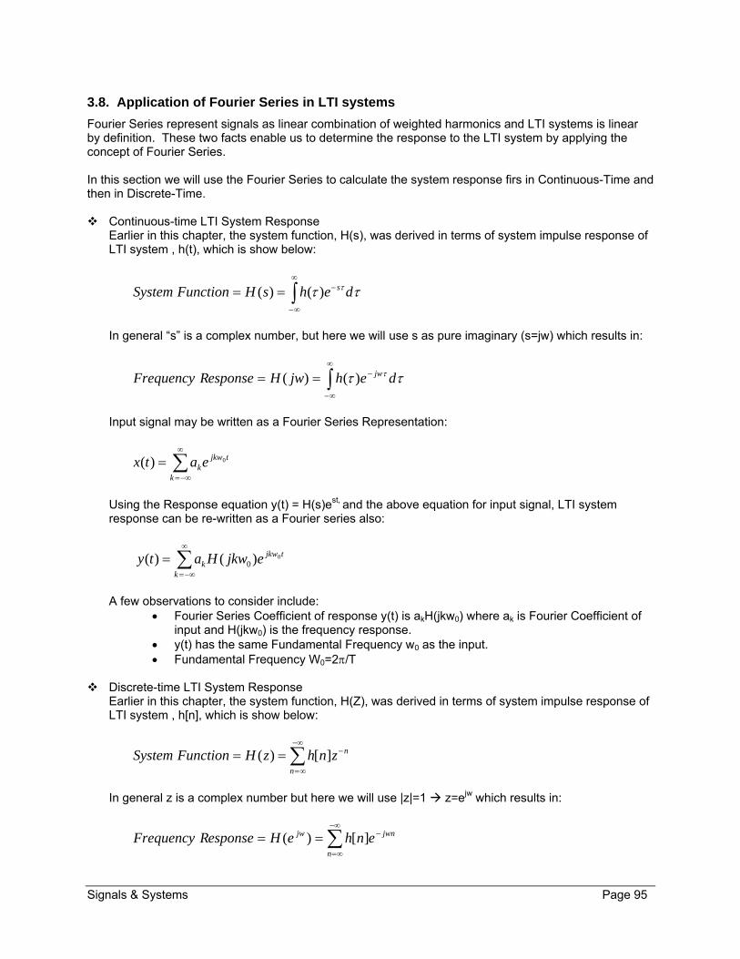
Signals & Systems Page 95
3.8. Application of Fourier Series in LTI systems
Fourier Series represent signals as linear combination of weighted harmonics and LTI systems is linear by definition. These two facts enable us to determine the response to the LTI system by applying the concept of Fourier Series. In this section we will use the Fourier Series to calculate the system response firs in Continuous-Time and then in Discrete-Time. Continuous-time LTI System Response
Earlier in this chapter, the system function, H(s), was derived in terms of system impulse response of LTI system , h(t), which is show below:
dehsHFunctionSystem s)()(
In general “s” is a complex number, but here we will use s as pure imaginary (s=jw) which results in:
dehjwHesponseRFrequency jw)()(
Input signal may be written as a Fourier Series Representation:
k
tjkwkeatx 0)(
Using the Response equation y(t) = H(s)est, and the above equation for input signal, LTI system response can be re-written as a Fourier series also:
k
tjkwk ejkwHaty 0)()( 0
A few observations to consider include:
Fourier Series Coefficient of response y(t) is akH(jkw0) where ak is Fourier Coefficient of input and H(jkw0) is the frequency response.
y(t) has the same Fundamental Frequency w0 as the input. Fundamental Frequency W0=2/T
Discrete-time LTI System Response
Earlier in this chapter, the system function, H(Z), was derived in terms of system impulse response of LTI system , h[n], which is show below:
n
nznhzHFunctionSystem ][)(
In general z is a complex number but here we will use |z|=1 z=ejw which results in:
n
jwnjw enheHesponseRFrequency ][)(

Signals & Systems Page 96
Input signal may be written as a Fourier Series Representation:
Nk
njkwkeanx 0][
Using the Response equation y[n] = H(z)zn, and the above equation for input signal, LTI system response can be re-written as a Fourier series also:
Nk
njkwjkwk eeHany 00 )(][
A few Observations to consider include:
Fourier Series Coefficient of response y[n] is akH(ejkw0) where ak is Fourier Coefficient of input and H(ejkw0) is the frequency response.
Y[n] has the same Fundamental Frequency w0 as the input. Fundamental Frequency W0=2/N
Examples – Application of Fourier Series in LTI Systems Properties Example – Signal, x(t) = 20 + 3 cos(3πt/8 – π/3), is passed through a low pass filter with cut off
frequency of 10 Hz. Write the output signal equation. Solution: response, y(t) = 20 + 3 cos(3πt/8 – π/3)
Example – x(t) is a square wave with the period of 1 msec. and 25% duty cycle with maximum of 5V and minimum of 0V. This signal is input to a band pass filter with cut off frequencies of 5,000 and 10,000 rad/sec. Calculate and plot the response in frequency and time domain. Solution:

Signals & Systems Page 97
3.9. Chapter Summary
This section is a summary of key concepts from this chapter. Continuous-Time Fourier Series x(t) must be periodic and converging.
k
tTjkk
k
tjkwk eaeatx )/2(0)(
Synthesis Equation
T
tTjk
T
tjkwk dttxe
Tdttxe
Ta )(
1)(
1 )/2(0 Analysis Equation
Discrete-Time Fourier Series X[n] must be periodic and is by definition converging.
1,...,1,
][ )/2(
Nmmmkfor
eaeanxNk
nNjkk
Nk
njkwk
o
Synthesis Equation
Nn
nNjk
Nn
njkwk enx
Nenx
Na o )/2(][
1][
1 Analysis Equation
Euler’s Identity
j
eea
eea
ajae
jaja
jaja
ja
2)sin(
2)cos(
)sin()cos(

Signals & Systems Page 98
3.10. Additional Resources
Oppenheim, A. Signals & Systems (1997) Prentice Hall Chapter 3.
Lathi, B. Modern Digital & Analog Communication Systems (1998) Oxford University Press Chapter 3.
Stremler, F. Introduction to Communication Systems (1990) Addison-Wesley Publishing Company Chapter 3.
Nilsson, J. Electrical Circuits. (2004) Pearson. Chapter 16 and 17.

Signals & Systems Page 99
3.11. Problems
Refer to www.EngrCS.com or online course page for complete solved and unsolved problem set.
Signals & Systems Page 100
Chapter 4. The Continuous-Time Fourier Transform
Key Concepts and Overview Introduction
Fourier Transform of Aperiodic and Periodic Signals
Fourier Transform Convergence
Properties of the Continuous-Time Fourier Transform
Systems Characterized by Linear Constant-Coefficient Differential Equations
Additional Resources

Signals & Systems Page 101
4.1. Introduction
This chapter introduces Fourier Transform for Aperiodic signals. We will leverage the work from pervious chapter on Fourier series for the periodic signal. Aperiodic signal will be approached as if it is a periodic signal with period, T . This would also imply that the fundamental frequency W0 0. The resulting Fourier Transform has a number of useful properties that will be used to describe the characteristics of the original signal. Additionally, the Fourier Transform plays an important role in study of signal & systems by providing a Frequency spectrum analysis tool. It will also be shown that Fourier Transform is also applicable to periodic signal. This chapter is dedicated to Continuous time signal and it’s Fourier Transform. Next chapter applies Fourier Transform to the Discrete-time aperiodic signals.

Signals & Systems Page 102
4.2. Fourier Transform for Aperiodic and Periodic Signals
The development of Fourier Transform for Continuous-time Aperiodic signals starts by revisiting the definition of Aperiodic signal. An Aperiodic signal has non zero value of interested from some time value T1 to T2 which would fit within an interval t0 to (t0 + T). As shown below:
We can consider that the signal shown above is a single period of a periodic signal with a period of T. With this consideration, the Continuous-Time Fourier Series synthesis and analysis equation can be used to write the following equations for x(t) approximation and ak:
dtetxT
a
eatx
T
T
tjkwk
tjkw
kk
2/
2/
0
0
)(1
)(
for the Interval: 0 t T where w0 = 2/T
Since the signal in reality is not periodic and the value of x(t) is zero outside of the interval, we can change the integration limit to infinity and use x(t) instead of approximation. These modifications results in the following analysis for calculation of Fourier Series Coefficient:
dtetxT
a tjkwk
0)(1
At this point we can define the Fourier Transform X(jw) as T multiplied by ak.
dtetxjwX jwt
)()( Fourier Transform or Fourier Integral of x(t)
From the above equation, the Fourier Series Coefficient for a periodic signal may be calculated by setting w to kw0 as shown below:
)(1
jwXT
ak where w = kw0
using the above two equations, we can write the x(t) approximation in-term of X(jw) as shown below:
tjkw
k
ejkwXT
tx 0)(1
)( 0
X(t)
t T2 T1

Signals & Systems Page 103
we know that wo = 2 /T or T =2 / wo so we can rewrite the above equation as:
dwejwXwejkwXtx jwt
k
tjkw
k
)(2
1)(
2
1)( 00
0
In the case of an Aperiodic signal, T, wo 0 and dw 0 which means the sum of terms in the above equation changes to an integral. This change results in the following integral which is referred to as an Inverse Fourier Transform:
dwejwXtx jwt)(2
1)(
Inverse Fourier Transform
Below is a summary of the three equations resulting from the above derivations:
periodiciftCoefficienSeriesFourierjkwXT
jwXT
a
txofegralFourierortransformFouriertxFdtetxjwX
equationtransformFourierInversejwXFdwejwXtx
ok
jwt
jwt
)(1
)(1
)(int)()()(
)()(2
1)( 1
Example: Continuous-Time Fourier Transform for Aperiodic Signals
Example 1 – Find the Fourier Transform for the signal x(t) =e-2t u(t).
Solutions:
jwjwX
ejw
dtedteedtetuejwX tjwtjwjwttjwtt
2
1)(
2
1)()( 0
)2(
0
)2(
0
22
Example 2 – Find the x(t) with Fourier Transform X(jw) = 5 2 < w < 4 0 Otherwise Solution:
)(2
55
2
1)(
2
1)( 24
4
2
tjtjjwtjwt eet
dwedwejwXtx
Example 3 - Find Fourier transform of the signal:
x(t) = e-a|t| u(t-1) – u(t-5) Solutions:

Signals & Systems Page 104
Student Exercise.
Example 3 - Find Fourier transform of the signal: x(t) = e-a|t| u(t+1) – u(t+5) Solutions: Student Exercise.
Fourier Transform of Periodic Signals The Fourier Transform of Continuous-time Aperiodic signal derivation can be extended to find the Fourier Transform of periodic signals. Let’s start with a Fourier Transform of the following form: X(jw) = 2δ(w-w0) We can apply inverse Fourier Transform to find x(t):
tjwjwtjwt edwewwdwejwXtx 0)(22
1)(
2
1)( 0
Note: δ(w-w0)f(w)=f(w0) We can generalize the above derivation to:
tjkwetx 0)( which has a Fourier Transform of the form X(jw) = 2δ(w-kw0)
As it was developed in the previous section, Periodic signals may be written as linear sum of their harmonic using Fourier Series Coefficients which is shown below:
tjkw
kk eatx 0)(
Using the above relationships, Fourier Transform of Periodic signal may be written as:
k
k kwwajwX )(2)( 0
The Fourier transform of a periodic signal with Fourier Series Coefficients aK is an impulse train at the harmonic frequencies. The impulse train will be used in later chapters for the analysis of sampling systems. Here is a summary of relationships for Fourier Transform of periodic signals:

Signals & Systems Page 105
EquationTransformFourierkwwajwX
EquationAnalysisSeriesFourierdtetxT
a
EquationSynthesisSeriesFouriereatx
kk
T
T
tjkwk
tjkw
kk
)(2)(
)(1
)(
0
2/
2/
0
0
Example 1– Find the Fourier Transform for the signal x(t) = sin(300t).
Solutions: w0 = 300 = 2/T T = 2/300
)]()([)(2)(
002
1
)(2
1
2
300
)300(sin2
300)(
1
000
11
300/
300/
300300300
300/
300/
3002/
2/
0
wwwwj
kwwajwX
kforaandj
aa
dteeej
a
dtetdtetxT
a
kk
k
tjktjtjk
tjkT
T
tjkwk
Example 2 – Find the Fourier Transform for a periodic square wave with 25% duty cycle a with the period of 10 uSec., high value of 2v and low of -1v. Solutions: Student Exercise

Signals & Systems Page 106
4.3. Fourier Transform Convergence
The discussion of the Continuous-Time Fourier Transform for Aperiodic signals convergence is similar to the convergence of Fourier Series for periodic signals. Fourier Transform of x(t) converges and the
equation
dwejwXtx jwt)(2
1)(
^
accurately represent the original signal x(t) only if x(t) has finite
energy as shown by the following equation:
dttxEnergy 2|)(|
If the original x(t) and x(t) approximated by inverse Fourier Transform have the same finite energy then the total error energy is 0 as shown below:
0|)(|
)()()(
2
dtteEnergy
txtxteerror
Another way to state the same concept is that “the approximated signal has the same energy signature as the original x(t) signal”. Much like the periodic case, Dirichlet conditions are sufficient to ensure the approximation of x(t) using Inverse Fourier Transform is equal to x(t) except at the discontinuities. As discussed earlier, the value at the discontinuities is equal to the average of the values on either side of discontinuity. Again, the three Dirichlet conditions required for convergence are listed here:
1) x(t) is absolutely integrateable which means
dttx |)(| .
2) x(t) has finite number of oscillations within any finite interval. 3) x(t) has finite number of discontinuities within any finite interval and each discontinuity is finite.

Signals & Systems Page 107
Example – Fourier Transform Convergence Example 1 – determine the Fourier Transform For the following signal if it converges:
x(t)=e-b|t| where b>0. Solution: Since all three of Drichelet’s condition holds, X(jw) converges and x(t) has a valid Fourier series. The following process is used to calculate x(jw):
22
0
0
2)(
11)()(
wb
bjwX
jwbjwbdteedteedtetxjwX jwtbtjwtbtjwt
t w
x(t)
1
-b b
1/b
X(jw)
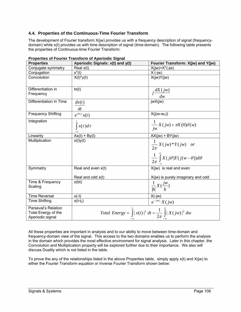
Signals & Systems Page 108
4.4. Properties of the Continuous-Time Fourier Transform
The development of Fourier transform X(jw) provides us with a frequency description of signal (frequency-domain) while x(t) provides us with time description of signal (time-domain). The following table presents the properties of Continuous-time Fourier Transform: Properties of Fourier Transform of Aperiodic Signal Properties Aperiodic Signals: x(t) and y(t) Fourier Transform: X(jw) and Y(jw) Conjugate symmetry Real x(t) X(jw)=X*(-jw) Conjugation x*(t) X*(-jw) Convolution X(t)*y(t) X(jw)Y(jw)
Differentiation in Frequency
tx(t)
dw
jwdXj
)(
Differentiation in Time
dt
tdx )(
jwX(jw)
Frequency Shifting )(txe tjwo X(j(w-w0))
Integration
t
dx )( )()0()(1
wXjwXjw
Linearity Ax(t) + By(t) AX(jw) + BY(jw) Multiplication x(t)y(t)
dwjYjX
orjwYjwX
))(()(2
1
)(*)(2
1
Symmetry Real and even x(t) Real and odd x(t)
X(jw) is real and even X(jw) is purely imaginary and odd
Time & Frequency Scaling
x(bt) )(
1
b
jwX
b
Time Reversal x(-t) X(-jw) Time Shifting x(t-t0) )( jwXe ojwt
Parseval’s Relation Total Energy of the Aperiodic signal
dwjwXdttxEnergyTotal 22 |)(|2
1|)(|
All these properties are important in analysis and to our ability to move between time-domain and frequency-domain view of the signal. This access to the two domains enables us to perform the analysis in the domain which provides the most effective environment for signal analysis. Later in this chapter, the Convolution and Multiplication property will be explored further due to their importance. We also will discuss Duality which is not listed in the table. To prove the any of the relationships listed in the above Properties table, simply apply x(t) and X(jw) to either the Fourier Transform equation or Inverse Fourier Transform shown below:
Signals & Systems Page 109
)(int)()()(
)()(2
1)( 1
txofegralFourierortransformFouriertxFdtetxjwX
equationtransformFourierInversejwXFdwejwXtx
jwt
jwt
Example – Fourier Transform
Example – Prove the frequency shifting Property of Fourier transform:
))(()( 0wwjXtxeF tjwo or ))(()( 01 wwjXFtxe tjwo
Solution:
Example2 – Using the properties in the properties table find the Fourier transform in terms of Fx(t)=X(jw) for the following signal: y(t) = 2 x(t - k/3) + 4 x(t + n/5) Solution:
Example – Find Fourier Transform of y(t) = )25()(
txdt
tdx when Fourier Transform of x(t)is
X(jw). Solution:
)()()( 25 jwXejwjwXjwY wj
Example – Find Fourier Transform of y(t) = ))25(200sin())2000(sin(
tdt
td .
Solution:

Signals & Systems Page 110
Convolution Property and Application Convolution property states that a time-domain convolution is replaced by multiplication in frequency domain as shown below:
)()()()()(*)()( jwHjwXjwYtyFtxthtyF
Here is the proof that Convolution Property holds true:
)()()(
)(2
1)(sin
)()(2
1)()(
2
1lim)(
sup
)()()()(
)(2
1lim)(
0
)(2
1)(
0000
0
000
0
0
0
0
0
0
jwHjwXjwY
Then
dwejwYtyce
dwejwHjwXwejkwHjkwXty
erpositionandproductsfrequencycrossnoassuchpropertiesLTIApplying
dtethjkwHdtethsH
wejkwXtx
kandwwhensumaasrewritecanyou
dwejwXtx
jwt
jwt
k
tjkw
w
tjkwst
k
tjkw
w
jwt
The importance of Convolution property is the fact that it can be applied to LTI systems to determine the System Response. In earlier work, it is known that in time-domain the system response is equal to input x(t) convoluted with impulse response h(t): y(t) = h(t) * x(t) By taking the Fourier Transform of both side, we can state that in frequency-domain, response Y(jw) is the product of input X(jw) and Frequency Response H(jw): Y(jw) = X(jw)H(jw) where X(jw) = Fx(t), Y(jw) = Fy(t) and H(jw) = Fh(t). Below is a system diagram annotated in time-domain and frequency-domain:
Like the unit impulse response, h(t), frequency response H(jw) completely characterizes the LTI System and it does not depend on the order. Therefore, the following system configurations are
LTI System h(t) “Impulse Response”
H(jw)=Fh(t) “Frequency Response”
x(t) X(jw) =Fx(t)
y(t) Y(jw) =Fy(t)

Signals & Systems Page 111
equivalent:
Furthermore, H(jw) converges and exists if its energy is bounded. This means we can apply Drichlet’s three conditions. If all three condition are met then H(jw) converges and therefore it exists:
x(t) is integrable; that is
dttx )(
x(t) has finite number of oscillation within any finite interval x(t) has finite number of discontinuities within any finite interval. Furthermore, each of
these discontinuities must be finite.
Example - Given dttxtyt
)()( is response of an LTI system with input x(t) what is the impulse
response h(t) of the LTI system? Solution:
Take an inverse Fourier transform of dttxtyt
)()(
)()(
sin
)(1
)(:
)()()(:
)()(1
)(
)()()(1
)(
)()()()0(:
)()0()(1
)(
tuth
tablepropertygu
wjw
jwHTherefore
jwHjwXjwYKnown
jwXwjw
jwY
wjwXjwXjw
jwY
wjwXwXknown
wXjwXjw
jwY
Multiplication Property and Application
Multiplication property states that a time-domain multiplication is replaced by convolution in frequency domain as shown below:
H1(jw) H2(jw) y(t) x(t)
H2(jw) H1(jw) y(t) x(t)
H1(jw) H2(jw) y(t) x(t)
Y(jw)=X(jw)H1(jw)H2(jw)
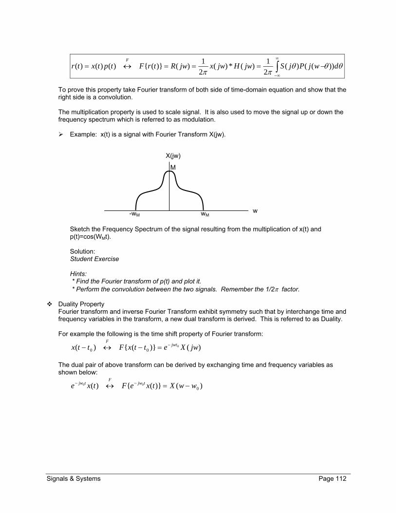
Signals & Systems Page 112
dwjPjSjwHjwxjwRtrFtptxtrF
))(()(2
1)(*)(
2
1)()()()()(
To prove this property take Fourier transform of both side of time-domain equation and show that the right side is a convolution. The multiplication property is used to scale signal. It is also used to move the signal up or down the frequency spectrum which is referred to as modulation. Example: x(t) is a signal with Fourier Transform X(jw).
Sketch the Frequency Spectrum of the signal resulting from the multiplication of x(t) and p(t)=cos(WMt). Solution: Student Exercise Hints: * Find the Fourier transform of p(t) and plot it. * Perform the convolution between the two signals. Remember the 1/2 factor.
Duality Property Fourier transform and inverse Fourier Transform exhibit symmetry such that by interchange time and frequency variables in the transform, a new dual transform is derived. This is referred to as Duality. For example the following is the time shift property of Fourier transform:
)()()( 000 jwXettxFttx jwt
F
The dual pair of above transform can be derived by exchanging time and frequency variables as shown below:
)()()( 000 wwXtxeFtxe tjw
Ftjw
w
X(jw)
M
-wM wM

Signals & Systems Page 113
Time-Domain Signal, Fourier Transform and Fourier Series Coefficient The following table summarizes some of the most common Signals and their Fourier transforms. Also included is the Fourier Series Coefficient for the signal if the signal is periodic.
Time-Domain Signal, Fourier Transform and Fourier Series Coefficient Signal, x(t) =F-1X(jw) Fourier Transform, X(jw)=Fx(t) [1] Fourier Series Coefficient, ak
tjkw
kkea 0
)(2 0kwwak
k
dtetxT
tjkw
0)(1
tjwe 0 )(2 0ww a1=1 ak =0 for all other k values
cos(w0t) )]()([ 00 wwww a1 = a-1 =1/2 ak =0 for all other k values
sin(w0t) )]()([ 00 wwww
j
a1 = -a-1 =1/(j2) ak =0 for all other k values
1 )(2 w a0= 1 ak =0 for all other k values
Periodic Square Wave x(t) = 1 |t| <T1 0 T1< |t| <T/2 with Period T.
)()sin(2
010 kww
k
Tkw
k
k
Tkw )sin( 10
Pulse Train in Time
n
nTt )(
k T
kw
T)
2(
2
ak = 1/T for all k
x(t) = 1 |t|<T1
0 |t|≥T1 w
wT1sin2
N.A.
t
Wt
sin
X(jw) = 1 |w| < W 0 |w| > W
N.A.
)(t 1 N.A.
u(t) )(
1w
jw
N.A.
)( 0tt 0jwte N.A.
)(tue at for Rea>0
jwa 1
N.A.
)(tute at for Rea>0 2)(
1
jwa
N.A.
)()!1(
1
tuen
t atn
for Rea>0
njwa )(
1
N.A.
Note: [1]Fourier Series Coefficient exists only if signal is periodic.
Signals & Systems Page 114
4.5. Chapter Summary
This section is a summary of key concepts from this chapter. Continuous -time Fourier Transform
x(t) may be aperiodic but must be converging. Fourier Transform - Analysis Equation
X(jw) is the Fourier Transform of x(t) and is aperiodic in frequency domain.
dtetxtxFjwX jwt)()()(
Fourier Inverse Transform - Synthesis Equation x(t) is the Fourier inverse Transform of x(t) and is aperiodic in time domain.
dwejwXtxFtx jwt)(2
1)()( 1
Fourier Transform and Fourier Series relationship (valid only if x(t) is periodic) ak =X(jw) = X(jkw0)

Signals & Systems Page 115
4.6. Additional Resources
Oppenheim, A. Signals & Systems (1997) Prentice Hall Chapter 4.
Lathi, B. Modern Digital & Analog Communication Systems (1998) Oxford University Press Chapter 3.
Stremler, F. Introduction to Communication Systems (1990) Addison-Wesley Publishing Company Chapter 3.
Nilsson, J. Electrical Circuits. (2004) Pearson. Chapter 16 and 17.

Signals & Systems Page 116
4.7. Problems
Refer to www.EngrCS.com or online course page for complete solved and unsolved problem set.

Signals & Systems Page 117
Chapter 5. The Discrete-Time Fourier transform
Key Concepts and Overview Introduction
Fourier Transform of Aperiodic and Periodic Signals
Fourier Transform Convergence
Properties of the Discrete-Time Fourier Transform
Summary of Fourier Series and Transform Equations
Systems Characterized by Linear Constant-Coefficient Differences Equations
Additional Resources

Signals & Systems Page 118
5.1. Introduction
As discussed earlier, a major benefit of Fourier Transform is the ability to perform Frequency-Domain analysis for LTI system in addition to time-domain analysis. Specifically, the convolution property in time-domain and its equivalent multiplication in frequency-domain relate the response and input of a LTI system. Development of Discrete-Time Fourier Transform for Aperiodic signals follows a similar process to the Continuous-Time Fourier Transform development. As it was done in the last chapter, the development of Discrete-Time Fourier Transform starts with the Fourier series and the assumption that any aperiodic signal can be treated as a single period of periodic signal. Many of the Discrete-Time Fourier Transform properties are counterparts of the Continuous-Timer Fourier Transform properties. One difference is that the Discrete-Time Fourier Transform of an aperiodic signal is always periodic with period 2.
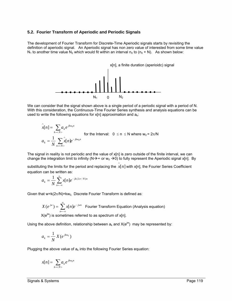
Signals & Systems Page 119
5.2. Fourier Transform of Aperiodic and Periodic Signals
The development of Fourier Transform for Discrete-Time Aperiodic signals starts by revisiting the definition of aperiodic signal. An Aperiodic signal has non zero value of interested from some time value N1 to another time value N2 which would fit within an interval n0 to (n0 + N). As shown below:
We can consider that the signal shown above is a single period of a periodic signal with a period of N. With this consideration, the Continuous-Time Fourier Series synthesis and analysis equations can be used to write the following equations for x[n] approximation and ak:
njkw
Nnk
njkw
Nkk
enxN
a
eanx
0
0
][1
][
for the Interval: 0 n N where w0 = 2/N
The signal in reality is not periodic and the value of x[n] is zero outside of the finite interval, we can change the integration limit to infinity (N∞ or w0 0) to fully represent the Aperiodic signal x[n]. By
substituting the limits for the period and replacing the with x[n], the Fourier Series Coefficient
equation can be written as:
n
nNjkk enx
Na )/2(][
1
Given that w=k(2/N)=kw0, Discrete Fourier Transform is defined as:
n
jwnjw enxeX ][)( Fourier Transform Equation (Analysis equation)
X(ejw) is sometimes referred to as spectrum of x[n]. Using the above definition, relationship between ak and X(ejw) may be represented by:
)(1
0jkwk eX
Na
Plugging the above value of ak into the following Fourier Series equation:
Nk
njkwk eanx 0][
][nx
0 N2 N1
x[n], a finite duration (aperioidc) signal
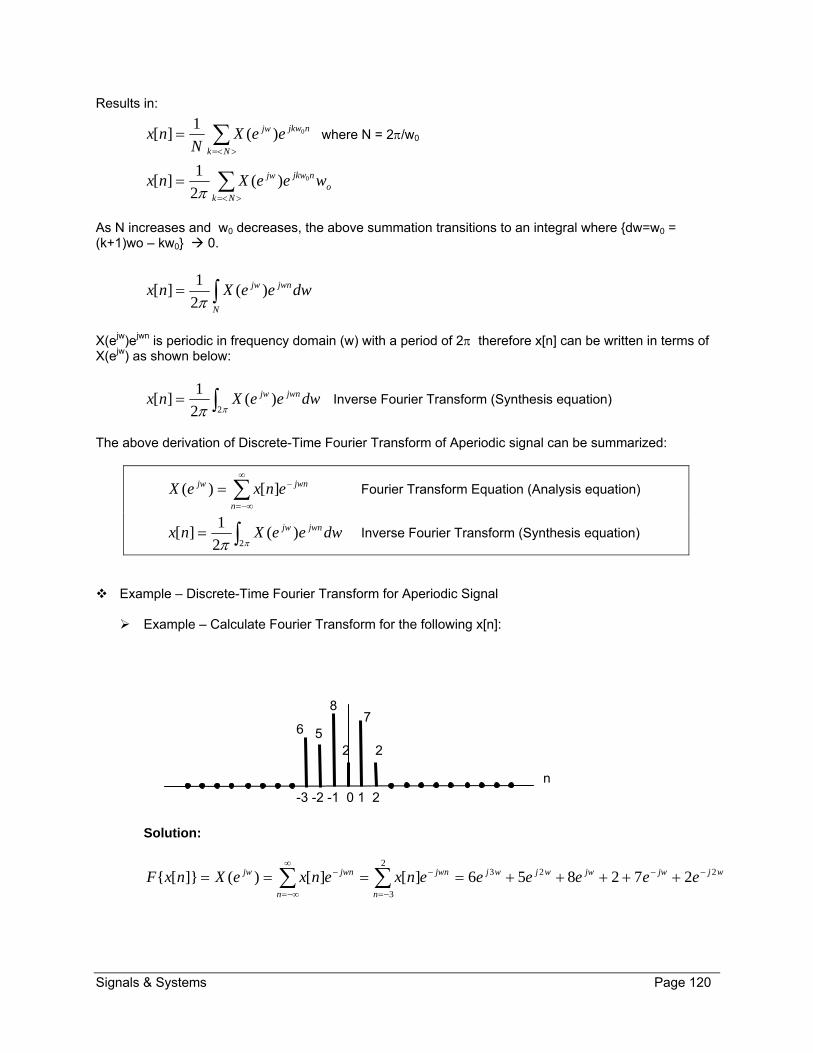
Signals & Systems Page 120
Results in:
Nk
njkwjw eeXN
nx 0)(1
][ where N = 2/w0
Nk
onjkwjw weeXnx 0)(
2
1][
As N increases and w0 decreases, the above summation transitions to an integral where dw=w0 = (k+1)wo – kw0 0.
N
jwnjw dweeXnx )(2
1][
X(ejw)ejwn is periodic in frequency domain (w) with a period of 2 therefore x[n] can be written in terms of X(ejw) as shown below:
dweeXnx jwnjw 2
)(2
1][ Inverse Fourier Transform (Synthesis equation)
The above derivation of Discrete-Time Fourier Transform of Aperiodic signal can be summarized:
n
jwnjw enxeX ][)( Fourier Transform Equation (Analysis equation)
dweeXnx jwnjw 2
)(2
1][ Inverse Fourier Transform (Synthesis equation)
Example – Discrete-Time Fourier Transform for Aperiodic Signal
Example – Calculate Fourier Transform for the following x[n]:
Solution:
wjjwjwwjwj
n
jwn
n
jwnjw eeeeeenxenxeXnxF 2232
3
272856][][)(][
-3 -2 -1 0 1 2
n
2
7 8
5 6
2

Signals & Systems Page 121
Example - Find and plot the magnitude and phase of Fourier Transform of x[n]=anu[n] where a<1. Solution
00
)(][][)(n
njw
n
jwnn
n
jwnn
n
jwnjw aeeaenuaenxeX
Applying the finite sum equation:
jwjw
aeeX
1
1)(
Plot the magnitude and phase of X(ejw) and use Matlab to plot the equation.
Example 2: Find and plot the magnitude and phase of Fourier Transform of x[n] = 1 where |n| ≤ N1 0 where |n| > N1 Solution
1
1
1
1
][)(N
Nn
jwnN
Nn
jwn
n
jwnjw eeenxeX
let n=m-N1
1
1
1
1
2
0
2
0
)()()(N
m
mjwjwNN
m
Nmjwjw eeeeX
Applying Finite Sum Equation
)2/sin(
)2/1(sin2
)(1
)(1)( 1
12 1
1
w
Nw
e
eeeX
jw
Njw
jwNjw
Plot the magnitude and phase of X(ejw) and use Matlab to plot the equation.
Fourier Transform of Discrete-Time periodic Signals
The remainder of this section is focused on derivation of Fourier Transform for Discrete-Time periodic
Signals. First, consider a periodic Signal njwenx 0][ which has a period of 2. We will suggest that
the Fourier Transform of x[n] should be sum of impulses at w0, w0 ± 2, w0 ± 4, … . So here is the Fourier Transform of x[n]:
l
jw lwweX )2(2][ 0
To check validity of the Fourier Transform, one has to take the Inverse Fourier Transform of X(ejw) and prove that x[n] is indeed a periodic signal:
njwjwn
l
jwnjw oedwelwwdweeXnx
2 02
)2(22
1)(
2
1][
Note : there is only one impulse per 2 period.

Signals & Systems Page 122
The general form of periodic signal (sequence) with period N and its transform can be written as follows:
kk
jw
Nk
nNjkk
N
kwaeX
eanx
)2
(2)(
][ )/2(
Fourier Transform of a periodic signal can be directly constructed from the Fourier Series Coefficients as shown by the above equation.
Example – Discrete-Time Fourier Transform of Periodic Signal
Example1: Find Fourier Transform of Periodic Signal: nwnx 0cos][ where 5
20
w .
Solution Apply Euler’s identity:
njwnjw oo eenx 2
1
2
1][
Now we can apply the Fourier Transform equation where5
20
w N=5
lll
jw lwlwlwweX )25
2(2
2
1)2
5
2(2
2
1)2(2][ 0
That is for each period (0 to 2) we have:
wwherewweX jw )5
2()
5
2(][
So the whole signal is shown below:
|X[ejw]|
w w0 -w0 0
(-2+w0) (-2-w0) -2 (2+w0) (2-w0) 2
. . . . . .

Signals & Systems Page 123
5.3. Fourier Transform Convergence
In the Discrete-Time Fourier Transform case, convergence is required in order for Fourier Transform to exist. This is another similarity between the Continuous-Time and Discrete-Time Fourier Transform. Here again we have to deal with infinite summation to find the Fourier Transform. So we need to ensure that the signal, x[n], is convergent before using the following Fourier Transform equation to find the Fourier Transform of x[n].
n
jwnjw enxeX ][)( Fourier Transform Equation
As discussed earlier, in order for xn] to be convergent and have a Fourier Transform, the following must be true:
n
nx |][| which says the xn] is absolutely summable
or
n
nx 2|][| which says that the sequence xn] has finite energy
In this case unlike the continuous-time situation we do not expect to see any behavior similar to the Gibbs Phenomenon since limits are finite. You may recall that Gibbs Phenomenon says that as the period increases, the ripples in the partial sums become compressed toward the discontinuity, but for any finite value of period, the peak amplitude of the ripples remains constant. Further, not all LTI systems have impulse responses that converge. For example 2nu[n] does not
converge since
n
notisnh |][| or diverges which means that it does not have a Fourier transform.
We will introduce an extension to Discrete-Time Fourier Transform called z-transform that will allow us to use the transformation techniques for LTI systems for which the frequency response does not converge. Finally, the issue of convergence does not exist for Inverse Fourier transform since the limits are defined within any 2 period:
dweeXnx jwnjw 2
)(2
1][ Inverse Fourier Transform

Signals & Systems Page 124
5.4. Properties of the Discrete-Time Fourier Transform
The development of Fourier transform X(ejw) provides us with a frequency description of signal (frequency-domain) while x[n] provides us with time description of signal (time-domain). The following table presents the properties of Discrete-time Fourier Transform: Properties of Discrete-Time Fourier Transform of Aperiodic Signal Properties
Aperiodic Signal x[n] and y[n]
Fourier Transform: X(ejw) and Y(ejw)
”always periodic with period 2” Linearity Ax[n] + By[n] AX(ejw) + BX(ejw) Time Shifting x[n – n0] )( jwjwn eXe o
Frequency Shifting ][nxe njwo )( )( owwjeX
Conjugation x*[n] X*(e-jw) Time Reversal x[-n] X(e-jw) Time Expansion x(k)[n] = x[n/k] if n = multiple of k
0 if n ≠ multiple of k X(ejkw)
Convolution x[n]*y[n] X(ejw)Y(ejw) Multiplication x[n]y[n]
deYeX
oreYeX
wjj
jwjw
)()(2
1
)(*)(2
1
)(
Differencing in Time x[n] – x[n – 1] (1 – e-jw)X(ejw) Summation
n
k
kx ][ )(1
1 jwjw
eXe
Differentiation in Frequency
nx[n]
dw
edXj
jw )(
Conjugate symmetry Real x[n] X(ejw)=X*(e-jw) Symmetry Real and even x[n]
Even x[n] Real and odd x[n]
X(ejw) is real and even X(ejw) is real X(ejw) is purely imaginary and odd
Parseval’s Relation Total Energy of the Aperiodic signal
2
22 |)(|2
1|][| dweXnxEnergyTotal jw
n
All these properties are important in analysis and to our ability to move between time-domain and frequency-domain view of the signal. This access to the two domains enables us to perform the analysis in the domain which provides the most effective environment for signal analysis. To prove that any of the relationships listed in the above Properties table, simply apply x[n] and X(ejw) to either the Fourier Transform equation or Inverse Fourier Transform shown below:
n
jwnjw enxeX ][)( Fourier Transform Equation
dweeXnx jwnjw 2
)(2
1][ Inverse Fourier Transform

Signals & Systems Page 125
Two important property to consider:
Periodicity: Discrete-time Fourier transform is always Periodic in w with period 2 for all x[n]
][][ 2 jwjw eXeX
Convolution: where y[n]=x[n]*h[n] and y(ejw)= X(ejw) H(ejw)
Example - Discrete-Time Fourier Transform Properties Example 1: Consider the following LTI system where the frequency response Hlp(e
jw) are ideal low pass filter with cutoff frequencies /4 and unity gain in the pass-band.
Find the Frequency response of the whole system. Solution
First work through the top path.
* We know that ))sin()(cos()1( njne njn
* We also know that this is a linear system therefore and applying frequency shifting property
)(][ )( 00 wwjnjw eXnxe )(
1 ()( wjjw eXeW
)()()()()()(
)()()()()()()()2()(
23
)(12
wj
lpjwwj
lpwjwjjw
jwlp
wjjwlp
jwjw
eHeXeHeXeWeW
eHeXeHeWeW
Now the bottom branch
)()()(4 jwlp
jwjw eHeXeW
X Hlp(ejw) X
Hlp(ejw)
x[n]
W1[n]
(-1)n
W2[n]
(-1)n
W3[n]
+
W4[n]
y[n]

Signals & Systems Page 126
Now the final addition of top and bottom branch:
)()()(
)()()()(
)()()()()()()(
)(
)(
)(43
wjlp
jwlp
jw
wjlp
jwlp
jwjw
wjlp
jwjwlp
jwjwjwjw
eHeHeH
Therefore
eHeHeXeY
eHeXeHeXeWeWeY
* We know )( jwlp eH is low pass filter with cut off frequency /4 Therefore
* ][)1()( )( nheH lpnwj
lp which is impulse response of high pass filter with cut off
frequency of 3/4 based on above two facts the system is a band pass filter with cut off frequencies at /4 and -/4 as shown below:
/4 -/4 -3/4 3/4
H(ejw)
w
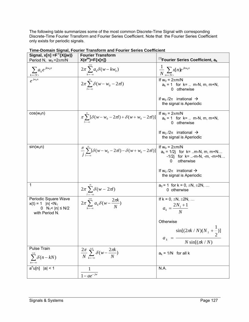
Signals & Systems Page 127
The following table summarizes some of the most common Discrete-Time Signal with corresponding Discrete-Time Fourier Transform and Fourier Series Coefficient. Note that the Fourier Series Coefficient only exists for periodic signals. Time-Domain Signal, Fourier Transform and Fourier Series Coefficient Signal, x[n] =F-1X(jw) Period N, w0 =2m/N
Fourier Transform X(ejw)=Fx[n] [1]Fourier Series Coefficient, ak
njkw
Nkk ea 0
)(2 0kwwak
k
njkw
Nn
enxN
0][1
njwe 0
l
lww )2(2 0 If w0 = 2m/N ak = 1 for k= .. m-N, m, m+N, 0 otherwise if w0 /2 irrational the signal is Aperiodic
cos(w0n)
l
lwwlww )]2()2([ 00
If w0 = 2m/N ak = 1 for k= .. m-N, m, m+N, 0 otherwise If w0 /2 irrational the signal is Aperiodic
sin(w0n)
l
lwwlwwj
)]2()2([ 00
If w0 = 2m/N ak = 1/2j for k= ..m-N, m, m+N… -1/2j for k= ..-m-N, -m, -m+N… 0 otherwise If w0 /2 irrational the signal is Aperiodic
1
l
lw )2(2 a0 = 1 for k = 0, N, 2N, … 0 otherwise
Periodic Square Wave x(t) = 1 |n| <N1 0 N1< |n| ≤ N/2 with Period N.
k
k N
kwa )
2(2
If k = 0, N, 2N, …
N
Nak
12 1
Otherwise
)/sin[(
)]2
1)(/2sin[( 1
NkN
NNk
a k
Pulse Train
n
kNn )(
k N
kw
N)
2(
2
ak = 1/N for all k
anu[n] |a| < 1 jwae1
1
N.A.

Signals & Systems Page 128
x[n] = 1 |N| ≤ N1
0 |N| > N1 )2/sin(
)2/1(sin2 1
w
Nw
N.A.
n
Wn
sin
0 < W < 1 for 0 ≤ |w| ≤ W 0 for W < |w| > X(ejw) is periodic with period of 2
N.A.
][n 1 N.A.
u[n]
kjw
kwe
)2(1
1 N.A.
][ 0nn 0jwne N.A.
][)1( nuan n |a|<1 2)1(
1jwae
N.A.
][)!1(!
)!1(nua
nn
rn n
|a|<1 rjwae )1(
1
N.A.
Note: [1]Fourier Series Coefficient exists only if signal is periodic.

Signals & Systems Page 129
5.5. Summary of Fourier Series and Transform Equations
This section is a summary of key concepts from this chapter. Discrete-time Fourier Transform
x(t) may be aperiodic but must be converging. Fourier Transform -Analysis Equation
X(ejw) is the Fourier Transform of x[n] and is periodic in frequency domain.
n
jwnjw enxnxFeX ][][)(
Fourier Inverse Transform -Synthesis Equation x(t) is the Fourier Inverse Transform of X(ejw) and is aperiodic in frequency domain.
2
1 )(2
1)(][ dweeXeXFnx jwnjwjw
Summary of Phase transform, Fourier series and Fourier Transform
Transform Time Domain (t) Frequency Domain (w) Phasor Transform x(t) a sinusoidal signal in steady
state system.
Fourier Series x(t) is periodic CT Signal xn] is periodic DT Signal
ak is periodic ak is periodic
Fourier Transform (s=jw)
x(t) is aperiodic CT Signal x[n] is aperiodic DT Signal
X(jw)=Fx(t) is aperiodic X(ejw)=Fx[ejw] is periodic
Laplace Transform (s=jw+σ)
x(t) is aperiodic CT Signal
X(jw)=Lx(t)
Z Transform (s=jw+σ)
xn] is aperiodic DT Signal X(z)=Zx[n]
The following table summarizes the Fourier Series and Transform relationships.
Continuous time Discrete time Time Domain Frequency
Domain Time Domain Frequency Domain
Fourier Series
k
tjkwk ea
tx
0
)(
Periodic in time
0
0)(1
0 T
tjkw
k
dtetxT
a
Aperiodic in freq.
Nk
nNjkkea
nx)/2(
][
Periodic in time
Nn
nNjk
k
enxN
a
)/2(][1
Periodic in frequency
Fourier Transform
dwejwX
tx
jwt)(2
1
)(
Aperiodic in time
dtetx
jwX
jwt)(
)(
Aperiodic in freq.
2
)(2
1
][
dweeX
nx
jwnjw
Aperiodic in time
n
jwn
jw
enx
ex
][
)(
Periodic in frequency

Signals & Systems Page 130
5.6. Additional Resources
Oppenheim, A. Signals & Systems (1997) Prentice Hall Chapter 5.
Lathi, B. Modern Digital & Analog Communication Systems (1998) Oxford University Press Chapter 3.
Stremler, F. Introduction to Communication Systems (1990) Addison-Wesley Publishing Company Chapter 3.
Nilsson, J. Electrical Circuits. (2004) Pearson. Chapter 16 and 17.

Signals & Systems Page 131
5.7. Problems
Refer to www.EngrCS.com or online course page for complete solved and unsolved problem set.

Signals & Systems Page 132
Chapter 6. Sampling
Key Concepts and Overview Introduction
Sampling Theorem
Aliasing Caused by Under Sampling
Interpolation Techniques for Signal Reconstruction From Samples
Statistical Approach to Sampling
Additional Resources

Signals & Systems Page 133
6.1. Introduction
This chapter focuses on sampling theory and its application to signals and systems. Natural signals such as images/light, sound/air pressure and movement are all continuous-time signals. This is of course true both in the sensing of this signal as well as control/generation of these types of signals. Prior to the advent of high speed computers and Fast Fourier Transform techniques, systems were designed to process the continuous-time signals directly, producing continuous-time output as depicted by the following diagram:
A filter build with active or passive electrical component is a good example of traditional continuous-time processing system. The flexibility of such systems are limited in-term of their ability to adapt to changing requirements of bandwidth, pass and no-pass transition time and cost. Additionally, it would be difficult to build systems that behave ideally with transitions that are instant such as in ideal filters. On the other hand, using the ability to convert the continuous-time (analog) input signal to discrete-time (digital) signals then processing it in discrete-time (digitally) and converting it back to continuous-time output (analog), enables designer to reduce cost while increase flexibility and precision. The following diagram graphically describes such a system.
With the advent of high speed computers and Fast Fourier Transforms techniques, this process delivers a more cost effective, flexible and precise system than direct continuous-time (analog) approach. Today, systems are designed using this approach except in cases where some unusual circumstance may exist. An example of unusual circumstance is extreme high conversions (sampling rate) requirements. Sampling rates of Giga samples per second is considered too high for this approach and it would be best designed in direct continuous-time. The key question that this chapter is concerned with is the conversion from continuous to discrete-time and back such that the original signal can be uniquely reconstructed. Sampling is the process of taking values of continuous-time signal at equal intervals and using them to construct a discrete time signal
Convert to Discrete-time signal using Analog-to-Digital (A/D) Converter
Continuous-time input, x(t)
Process the signal in Discrete-time (Digitally) using computer programs
Convert to Continuous-time signal using Digital-to-Analog (D/A) Converter
Continuous-time output, y(t)
Sampled Input xp(t)=x[n]
Sampled Output y[n]
Continuous-time signal Processing System
Continuous-time output Signal
Continuous-time input signal

Signals & Systems Page 134
representing the original signal. First question to be answered in this chapter is how many samples per seconds are required for complete reconstruction which leads to the Sampling Theorem. In the next section, Sampling Theorem is introduced. The Sampling Theorem is a critical element in system design since it is the bridge between continuous-time and discrete-time.

Signals & Systems Page 135
6.2. Sampling Theorem
Let‘s start by accepting the fact that a signal may not be uniquely specified by a sequence of equally spaced samples. For example, it is clear that x1(t) x2(t) x3(t) but the samples at equally spaced intervals are equal. x1(kT) = x2(kT) = x3(kT) as shown below:
However if the signal is band-limited which means the value of signal above a finite frequency is equal to 0, and we sample the signal at short enough intervals then the samples uniquely represent the signal. Let’s explore the previous sentence in more detail: First, signal is band-limited. This means that maximum frequency of the signal may be represented with a finite value WM. In other words, the Fourier Transform of signal at frequencies above WM is equal to 0. Second, the sample must be high enough frequency (short intervals) which we show latter means that the sample frequency, WS, must be more than twice the maximum signal frequency, WM . This key concept is known as Sampling Theorem. If Sampling Theorem conditions are met then the samples uniquely specify the signal, and we can reconstruct it perfectly. Now, let’s focus on the process of sampling a continuous-time signal. You may recall from earlier chapters, the concept of an Impulse Train Signal, p(t):
n
nTttp )()(
The impulse train signal is used to sample the signal. Basically, regularly space impulses are applied to the signal x(t) to obtain the sampled sequence as shown below:
)()()( tptxtx p where Impulse Train
n
nTttp )()(
T
x1(t)
x2(t)
x3(t)
Sample at kT
Sample at (k-1)T
Sample at (k-2)T
Sample at (k+1)T
Sample at (k+2)T
t
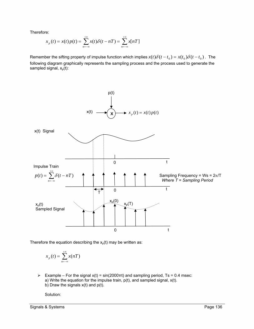
Signals & Systems Page 136
Therefore:
nn
p nTxnTttxtptxtx ][)()()()()(
Remember the sifting property of impulse function which implies )()()()( 000 tttxtttx . The
following diagram graphically represents the sampling process and the process used to generate the sampled signal, xp(t):
Therefore the equation describing the xp(t) may be written as:
n
p nTxtx )()(
Example – For the signal x(t) = sin(2000πt) and sampling period, Ts = 0.4 msec: a) Write the equation for the impulse train, p(t), and sampled signal, x(t). b) Draw the signals x(t) and p(t). Solution:
Xx(t)
p(t)
)()()( tptxtx p
0
0
0
T
xp(0) xp(T)
t
t
t
x(t) Signal
xp(t) Sampled Signal
Sampling Frequency = Ws = 2/T Where T = Sampling Period
Impulse Train
n
nTttp )()(

Signals & Systems Page 137
Student Exercise.
Applying the Multiplication property from Continuous-Time Fourier Transform Property:
dwjPjXjwPjwXjwX p ))(()(2
1)(*)(
2
1)(
Remember that the following two facts:
1) Fourier Transform of p(t) is
k
skwwT
jwP )(2
)( Note: Ws = 2/T
2) Convolution of impulse function and X(jw) results in a shifted signal X(jw) as shown below:
))(()(*)( 00 wwjXwwjwX
Using the above two facts in combination with Xp(jw), we can rewrite the sampled signal equation as:
k
sp kwwjXT
jwX ))((1
)(
Now that we have the Fourier Transform of the sampled signal in terms of the Fourier Transform of the shifted original signal, we can explore the signal and sampling in frequency spectrum. This view provides the basis to discuss the implication of the equation:
k
sp kwwjXT
jwX ))((1
)(
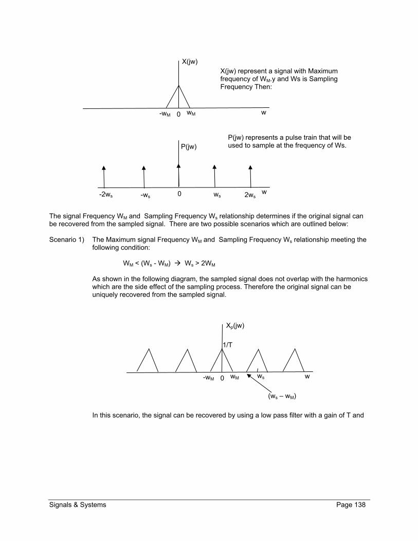
Signals & Systems Page 138
The signal Frequency WM and Sampling Frequency Ws relationship determines if the original signal can be recovered from the sampled signal. There are two possible scenarios which are outlined below: Scenario 1) The Maximum signal Frequency WM and Sampling Frequency Ws relationship meeting the
following condition: WM < (Ws - WM) Ws > 2WM
As shown in the following diagram, the sampled signal does not overlap with the harmonics which are the side effect of the sampling process. Therefore the original signal can be uniquely recovered from the sampled signal.
In this scenario, the signal can be recovered by using a low pass filter with a gain of T and
0 w
Xp(jw)
wM -wM
(ws – wM)
ws
1/T
0 w
0 w
X(jw)
P(jw)
wM -wM
-ws -2ws 2ws ws
X(jw) represent a signal with Maximum frequency of WM.y and Ws is Sampling Frequency Then:
P(jw) represents a pulse train that will be used to sample at the frequency of Ws.

Signals & Systems Page 139
cut-off frequency greater than WM and less than (Ws - WM).
Scenario 2) The Maximum signal Frequency WM and Sampling Frequency Ws relationship meeting the
following condition: WM ≥ (Ws - WM) Ws ≤ 2WM
As shown in the following diagram, the sampled signal overlaps with the harmonics of the original signal which results in a side effect refers to aliasing. This means that content of an alias (Harmonic) is corrupting the original signal spectrum. Therefore the original signal cannot be uniquely recovered from the sampled signal. Below is frequency spectrum of sampled signal under aliasing scenario:
This leads us to the Nyquist-Shannon Sampling Theorem or simply Sampling Theorem which are stated below:
If the signal x(t) is band-limited (X(jw)=0 for |w| > WM), then the signal x(t) is completely (uniquely) determined by its samples x(nT) only if Ws > 2WM.
Notes: [1] sampling frequency, Ws = 2/T. [2] n=0, 1, 2, …
The frequency 2WM, which, under the Sampling Theorem, must be exceeded by the sampling frequency, is commonly referred to as the Nyquist Rate. Nyquist Frequency refers to WM which is one half of the Nyquist Rate. The process to sample a continuous-time signal under the Sampling Theorem can be accomplished by multiplying the continuous-time signal x(t) with an impulse train signal p(t) to generate the sampled signal xp(t). Assuming the condition of Sampling Theorem is met (Ws > 2WM) then the original signal can be uniquely reconstructed using an ideal low pass filter with cut-off frequency wc between WM & Ws. Below is an example of the process used for sampling a continuous signal and then reconstructing the signal from the samples using a low pass filter (this example meets the sampling theorem requirement of
0 w
Xp(jw
wM -wM
(ws – wM)
ws
1/T
0 w
Xp(jw)
wM -wM ws
1/T
Ideal filter to recover the original signal.

Signals & Systems Page 140
Ws > 2WM):
This example uses an ideal low pass filter to recover the signal. Since real filters will not have the exact characteristic of an ideal low pass filter which means that there may be distortion in the reconstructed signal depending on how closely the recovery low pass filter matches the characteristic of an ideal low pass filter. Just a quick reminder that ideal low pass filter meets the following conditions: H(jw) = 1 for |w| < wM
0 for |w| > (ws – wM)
0 w
X(jw), Original Signal
wM -wM
0 w
Xp(jw), Signal Samples
wM -wM
(ws – wM)
ws
1/T
X x(t)
p(t)
Sampled Signal xp(t) Hlp(jw)
1
Recovered Signal Xr(t)
Sampling Recovery
0 w
Xr(jw), fully recovered Signal
wM -wM
1
Using sampling rate, ws the satisfies ws > 2 wM.
0 w
Hlp(jw), Ideal Low Pass Filter Transfer Function
Wc -wc
1 Cut-off frequency, wc Satisfies: wM < wc < (ws – wM)

Signals & Systems Page 141
The process of sampling described earlier requires the use of impulse train. Impulse function is a pulse of zero duration but finite amplitude. Of course, creating a signal that approaches impulse function definition is difficult even though the impulse function was useful in the process of arriving at the Sampling Theorem. A more practical approach to sampling is a method called “ Sampling with a zero-order hold”. Zero-order hold system samples x0(t) at a given instant and holds that value until next instant at which another sample is taken. Here is an illustration:
t
x(t)
X x(t)
p(t)
xp(t) Zero-hold sampled signal Xo(t)
Sampling
t
h0(t)
1
Ts
t
xp(t) – using impulse train
t
x0(t) – using zero-hold approach

Signals & Systems Page 142
Example – For the signal, x(t), with only nonzero coefficients (a0 -=1, a1=2, a3=2j) with
fundamental frequency of 22 Khz. a) What is the maximum frequency of signal x(t)? b) What are the nyquist frequency and rate? c) What is the Minimum and maximum sampling period so that x(t) is recoverable? d) What is the Minimum and maximum sampling frequency so that x(t) is recoverable? Solution:
Example – What is the minimum sampling frequency, fs, so that x(t)=sin(2000πt) is recoverable. Solution:

Signals & Systems Page 143
The Sampling and Recovery for the Zero-order hold system is as follows:
h0(t) is a square wave with duration from –T/2 to T/2 (shifted by T/2) therefore its Fourier Transform Function (using Fourier Transform Tables) can be written as:
w
wTejwH jwT )2/sin(2
)( 2/0
The next step is to find the frequency response for the reconstruction filter, Hr(jw). As we saw earlier a low pass filter was sufficient to recover x(t) from xp(t) which means the following relationships has to be true:
)(
)()()()()(
00 jwH
jwHjwHjwHjwHjwH lp
rrlp
Substituting the value of H0(jw) in the Hr(jw) results in the following equation:
w
wTjwHe
jwH lpjwT
r )2/sin(2)(
)(2/
With the Hlp(jw) cut off frequency equal to Ws/2, the ideal magnitude and phase for the reconstruction filter following a zero-order hold is shown below:
X x(t)
p(t)
xp(t) x0(t)
Sampling
t
h0(t)
1
T
hr(t)
Hr(jw)
Recovered Signal x(t)
Recovery (Reconstruction Filter)
Hlp(jw)
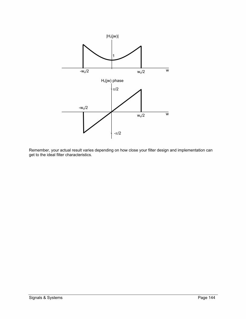
Signals & Systems Page 144
Remember, your actual result varies depending on how close your filter design and implementation can get to the ideal filter characteristics.
w
|Hr(jw)|
ws/2-ws/2
w
Hr(jw) phase
ws/2
-ws/2
/2
-/2
1

Signals & Systems Page 145
6.3. Aliasing Caused by Under Sampling
As Sampling Theorem states Sampling frequency (ws) must at least two times the maximum signal frequency (wM) in order to be able to completely reconstruct the original signal. In other words, the
reconstructed signal xr(t) will be equal to the original signal. Ms ww 2
If above conditional is violated, Ms ww 2 , then xr(t) is no longer equal to x(t), even though, the sample
values are equal to the original signal at the point of sample xr(nT)= x(nT). Let’s use x(t)=cos(w0t) to demonstrated the idea of aliasing. The Fourier Transform of x(t) can be written as: X(jw) = [(w - w0) + (w + w0)] Based on the equation for the Fourier Transform, we can draw the frequency spectrum of cos(w0t) as:
Depending on the Sampling frequency, we can have full recovery or aliasing defects in the reconstructed signal preventing full recovery. Below are examples of the two scenarios:
No Aliasing Scenario - Sampled at frequency ws = 4 wo In this case the maximum signal frequency is wm which is equal to wo therefore ws > 2 wm meeting the requirement of sampling theorem.
The time domain implication is that the original signal can be fully recoverable. Time-domain of
w0 -ws
Ideal low pass filter response overlay with cut off frequencies wc=ws/2.
w ws/2 ws
(ws - w0) (Ws + W0)
Xp(jw), Sampled Signal ws=4w0 =4 wM
X(jw), Original Signal (Dashed line is for –w)
w0 -w0
w
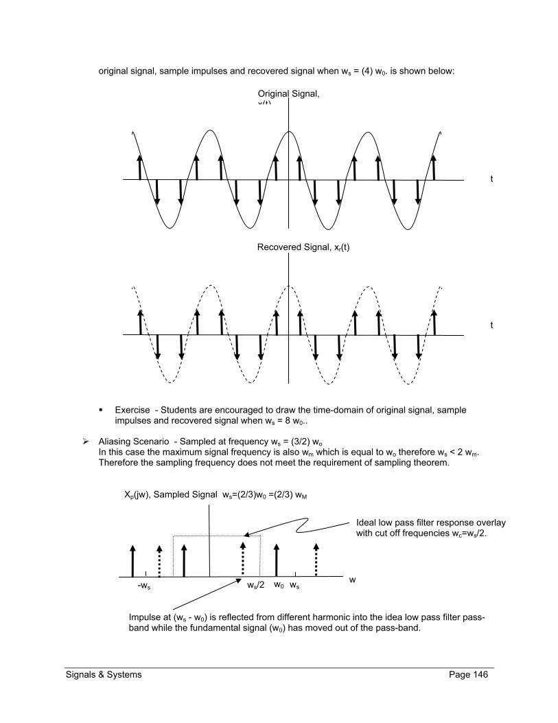
Signals & Systems Page 146
original signal, sample impulses and recovered signal when ws = (4) w0. is shown below:
Exercise - Students are encouraged to draw the time-domain of original signal, sample
impulses and recovered signal when ws = 8 w0..
Aliasing Scenario - Sampled at frequency ws = (3/2) wo
In this case the maximum signal frequency is also wm which is equal to wo therefore ws < 2 wm. Therefore the sampling frequency does not meet the requirement of sampling theorem.
w0 -ws w
ws/2 ws
Impulse at (ws - w0) is reflected from different harmonic into the idea low pass filter pass-band while the fundamental signal (w0) has moved out of the pass-band.
Xp(jw), Sampled Signal ws=(2/3)w0 =(2/3) wM
Ideal low pass filter response overlay with cut off frequencies wc=ws/2.
t
Original Signal, x(t)
t
Recovered Signal, xr(t)

Signals & Systems Page 147
In this case the original signal cannot be uniquely recovered. Time-domain of original signal, sample impulses and recovered signal when ws = (3/2) w0. is shown below:
Exercise - Students are encouraged to draw the time-domain of original signal, sample
impulses and recovered signal when ws = 2 w0.
observations As the w0 increases the dashed lines move to the right and solid lines move to the left. If frequency is increased so that w0 > ws/2 then aliasing will occur. It is important to note that the sampling frequency must be greater than twice the maximum signal frequency; even equal results in aliasing.
t
Original Signal, x(t)
t
Recovered Signal, xr(t)

Signals & Systems Page 148
6.4. Interpolation Techniques for Signal Reconstruction From Samples
In previous sections, we developed and discussed the Sampling Theorem and used it to sample continuous-time signals such that the sampled signal had sufficient information to fully recover the original signal from it. Further, it was shown that low pass filter would allow full recovery of the original signal without any aliasing as shown below again:
In other words, for band-limited signals, if the sampling rate is higher the twice the maximum frequency of signal, the signal can be constructed uniquely using Low Pass Ideal Filter. The challenge is that although it is possible to approximate an ideal low pass filter, it is impossible to implement an ideal low pass filter. Interpolation is an attempt to fit a continuous-time signal to a set of samples that approximates the original function. Two of the simplest interpolations are:
1) zero-order hold which simply holds the last sampled value of the signal until it is time for the next signal sample.
2) one-order hold or linear interpolation uses a straight line from one sample to next sample to approximate the original signal. There are higher-order hold approaches which use higher order polynomials to approximate between the two samples.
One way to compare the two basic reconstruction approaches (zero-order hold and first-order hold) is by comparing their transfer function with an ideal low pass filter:
0 w
Xp(jw), Signal Samples
wM -wM
(ws – wM)
ws
1/T
0 w
Xr(jw), fully recovered Signal
wM -wM
1
0 w
Hlp(jw), Low Pass filter transfer
Wc -wc
1 Cut-off frequency, wc Satisfies: wM < wc < (ws – wM)

Signals & Systems Page 149
As it is shown in the above responses, both zero-order and first-order hold have potential for aliasing which may distorts the reconstruction. By revisiting the process of ideal interpolating (low pass filter), we can describe the reconstructed signal xr(t) in terms of the ideal low pass filter characteristics as shown below:
n c
ccr
c
cc
cLP
nr
np
pr
nTtw
nTtwTwnTxtx
Finally
tw
twTwththerefore
otherwisewwforjwHknowwe
sposamplesbetweencurvecontinousfittohowshowsequationThis
nTthnTxtx
thereforenTtnTxtxhadweearlier
thtxtx
)(
))(sin()()(
,
)sin()(
0||1)(
int
)()()(
)()()(
)(*)()(
Interpolation using impulse response of low pass filter is commonly referred to as band-limited interpolation, since it implements exact reconstruction of x(t) is band limited and the sampling frequency satisfies the sampling frequency (ws>2wc). The zero-hold process was described in pervious section so at this point, we will explore the first-order hold which although more complex than zero-hold, it is simple enough to implement and provide improved approximation of the original signal: First-order hold or Linear Interpolation which means that Xp(t) is convoluted with h(t) that is linear in the form of a triangle. With the transfer function:
2
2/
)2/sin(1)(
w
wT
TjwH
H(jw)
w ws -ws -ws/2 ws/2
Ideal Interpolation “Ideal Low Pass Filter”
First-order Interpolation
Zero-order Interpolation
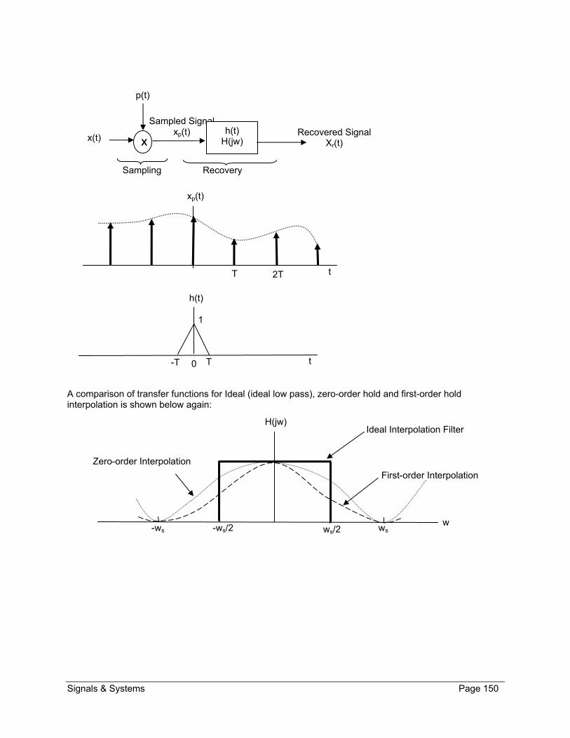
Signals & Systems Page 150
A comparison of transfer functions for Ideal (ideal low pass), zero-order hold and first-order hold interpolation is shown below again:
H(jw)
w ws -ws -ws/2 ws/2
Ideal Interpolation Filter
First-order Interpolation
Zero-order Interpolation
0 t
h(t)
T -T
X x(t)
p(t)
Sampled Signal xp(t) h(t)
H(jw)
1
Recovered Signal Xr(t)
Sampling Recovery
t T 2T
xp(t)

Signals & Systems Page 151
6.5. Additional Resources
Oppenheim, A. Signals & Systems (1997) Prentice Hall
Chapter 7. Lathi B. Modern Digital & Analog Communication Systems (1998) Oxford University Press
Chapter 6.

Signals & Systems Page 152
6.6. Problems
Refer to www.EngrCS.com or online course page for complete solved and unsolved problem set.

Signals & Systems Page 153
Chapter 7. Communication Systems
Key Concepts and Overview Introduction
Amplitude Modulation (AM)
Sinusoidal Amplitude Demodulation - Synchronous and Asynchronous
Frequency-Division and Time Division Multiplexing
Frequency Modulation(FM)
Additional Resources
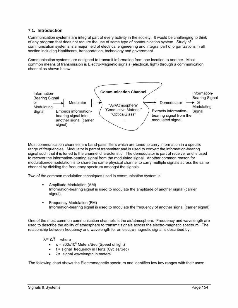
Signals & Systems Page 154
7.1. Introduction
Communication systems are integral part of every activity in the society. It would be challenging to think of any program that does not require the use of some type of communication system. Study of communication systems is a major field of electrical engineering and integral part of organizations in all section including Healthcare, transportation, technology and government. Communication systems are designed to transmit information from one location to another. Most common means of transmission is Electro-Magnetic signals (electrical, light) through a communication channel as shown below:
Most communication channels are band-pass filters which are tuned to carry information in a specific range of frequencies. Modulator is part of transmitter and is used to convert the information-bearing signal such that it is tuned to the channel characteristic. The demodulator is part of receiver and is used to recover the information-bearing signal from the modulated signal. Another common reason for modulation/demodulation is to share the same physical channel to carry multiple signals across the same channel by dividing the frequency spectrum amongst the signals. Two of the common modulation techniques used in communication system is:
Amplitude Modulation (AM) Information-bearing signal is used to modulate the amplitude of another signal (carrier signal).
Frequency Modulation (FM) Information-bearing signal is used to modulate the frequency of another signal (carrier signal)
One of the most common communication channels is the air/atmosphere. Frequency and wavelength are used to describe the ability of atmosphere to transmit signals across the electro-magnetic spectrum. The relationship between frequency and wavelength for an electro-magnetic signal is described by:
= c/f where c = 300x106 Meters/Sec (Speed of light) f = signal frequency in Hertz (Cycles/Sec) = signal wavelength in meters
The following chart shows the Electromagnetic spectrum and identifies few key ranges with their uses:
Modulator
Information- Bearing Signal or Modulating Signal
Demodulator
Communication Channel
”Air/Atmosphere” ”Conductive Material”
”Optics/Glass” …
Extracts information-bearing signal from the modulated signal.
Embeds information-bearing signal into another signal (carrier signal)
Information- Bearing Signal or Modulating Signal

Signals & Systems Page 155
Below is the profile of atmosphere response or opacity to signals based on frequency range:
Other channels such as glass-fiber optics, metal-transmission lines or space have their own unique opacity profile (response) with respect to various signal frequencies. Let’s start by considering a basic simplex system which is shown below with its components:
The word simplex refers to the fact that data only travels in one direction. The role of each component is described below:
Encoder Modulator Transmission
Medium Demodulator Decoder
Transmitter Channel Receiver
Information In (Signal)
Information Out (Signal)
Atmosphere Opacity
Radio Window f: 3x10⁵ to 3x10¹¹ Hz : 103 to 10-3 Meters
Optical Window f: 3x10¹³ to 3x10¹⁵ Hz : 10-5 to 10-7 Meters
Atmosphere is Opaque
Red Violet
103 107 1011 1015 1019 1023Frequency, c (Hertz)
3x10⁵ 3x101 3x10⁻³ 3x10⁻⁷ 3x10-11 3x10-15Wavelength, (Meters)
Radio AM540-1650 KHz; FM88-108 MHz; Microwave
Infrared far Near
Visible Freq :3 - 7.5x10¹⁴ Hz; Wavelength: 700 – 400 nanoMeter
Ultraviolet Near Far X rays
Soft Hard
Gamma rays
Scale Mount
Everest Human Height
Virus Atomic Nucleus
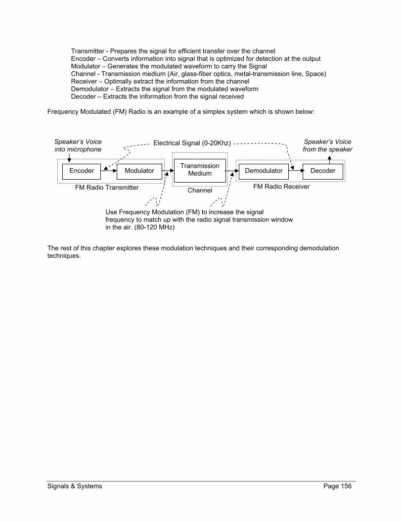
Signals & Systems Page 156
Transmitter - Prepares the signal for efficient transfer over the channel Encoder – Converts information into signal that is optimized for detection at the output Modulator – Generates the modulated waveform to carry the Signal Channel - Transmission medium (Air, glass-fiber optics, metal-transmission line, Space) Receiver – Optimally extract the information from the channel Demodulator – Extracts the signal from the modulated waveform Decoder – Extracts the information from the signal received Frequency Modulated (FM) Radio is an example of a simplex system which is shown below:
The rest of this chapter explores these modulation techniques and their corresponding demodulation techniques.
Encoder Modulator Transmission
Medium Demodulator Decoder
FM Radio Transmitter Channel FM Radio Receiver
Speaker’s Voice into microphone
Speaker’s Voice from the speaker
Electrical Signal (0-20Khz)
Use Frequency Modulation (FM) to increase the signal frequency to match up with the radio signal transmission window in the air. (80-120 MHz)

Signals & Systems Page 157
7.2. Amplitude Modulation (AM)
As discussed in the introduction, modulation is used to move the signal to a frequency range that is available and effective in the selected communication channel. For example, AM radio is typically broadcasted in frequencies from 500 Khz to 2 Mhz. Human audible signal frequency range is within 20 Hz - 20 Khz range. So the recorded signal x(t) has to modulated using a carrier signal c(t) in order to generated modulated signal y(t)=x(t)c(t) for transmission. Below is system diagram of a Modulator:
In Amplitude Modulation (AM), the signal we want to transmit (Information-bearing signal) x(t) is used to modulate the amplitude of the carrier signal, c(t). The carrier signal typically is either a complex exponential signal or a sinusoidal signal as shown below:
tjwcetc )( Complex exponential carrier signal
)cos()( twtc c Sinusoidal carrier signal
In both cases, wc is the Carrier Frequency and the carrier phase is assumed to be zero for simplicity. For the first case, let’s use the complex exponential carriers and apply it to the information bearing signal in order to obtain the equation for the modulated signal:
))(()(
:int
)(2)()(
)(()(2
1)(
)()(
)(
c
c
tjw
tjw
wwjXjwY
getweegrationnConvolutioabovethetoimplusetheApplying
wwtcFjwCGiven
dwjCjXjwY
propertyionmultipicatTransformFourierApplying
etxty
etcLetc
c
From the results, we can conclude that the modulated signal y(t) is information-bearing signal x(t) shifted
Information-bearing Signal, x(t) ”Modulating Signal”
Complex exponential or sinusoidal signal, c(t) ”Carrier Signal”
y(t)=x(t)c(t) ”Modulated Signal” X

Signals & Systems Page 158
by the carrier frequency wc which is shown below graphically:
On the receiving end, the information bearing signal can be recovered by demodulating the signal which means shifting the signal back. Here are the mathematical equivalents of demodulation:
))(()(
)()(
c
tjw
wwjyjwX
or
etytx c
The exponential carrier signal has real cosine and imaginary sine part (Application of Euler’s relationship). Typically the actual implementation requires the use of the following system:
X(jw)
w
w
C(jw)
wM wM
Y(jw)
w (wc + wM)
wc
wc (wc - wM)

Signals & Systems Page 159
It would be equally effective to only use one of the two paths shown above to modulate and demodulate signals. And, designer commonly use the sinusoidal carrier signal x(t)=cos(wct) to modulate the signal and simplify the communication system and has equally effective solutions.
Below are the derivations for the Fourier transform of the modulated signal Y(jw) when the sinusoidal carrier signal c(t) is used:
)(()((2
1)(
:int
)(()(2
1)(
)cos()()(
)()()()(
)cos()(
cc
c
cc
c
wwjXwwjXjwY
getweegrationnConvolutiothetoimplusetheApplying
dwjCjXjwY
propertyionmultipicatTransformFourierApplying
tjwtxty
wwwwjwCtcFGiven
tjwtcLet
From the results, we can conclude that the modulated signal y(t) is information-bearing signal x(t) shifted
X
c(t)= cos(wct)
Modulator
y(t) = x(t)c(t)= x(t)cos(wct) x(t))
x(t)
X
X
sin(wct)
cos(wct)
Imagy(t)
Realy(t)
X
X
-sin(wct)
cos(wct)
x(t)
Modulator Synchronous Demodulator

Signals & Systems Page 160
by the carrier frequencies - wc and +wc which is shown below:
When using sinusoidal Amplitude Modulation, it is required that wc > wM (Carrier Freq > Max. Signal Freq.) in order for the information-bearing signal to be recoverable. As it can be seen from the diagram, if wc ≤ wM then there will be an overlap between two replicas which mean that the information-bearing signal x(t) is not recoverable from the modulated signal y(t). The following diagram provides a time-domain representation of the Amplitude Modulation process:
X x(t)
cos(wct)
y(t)=x(t)cos(wct)
Antenna
t
x(t)
t t
c((t)=cos(wct)
a) Information-Bearing Signal, x(t)
b) Carrier Signal, c(t) c) Modulated Signal, y(t)
X(jw)
w wM wM
C(jw)
w wc -wc
Y(jw)
w wc (-wc -wM) -wc (-wc + wM) (wc -wM) (wc + wM)
1/2
1

Signals & Systems Page 161
Example – Available Modulator/Demodulator (Modems) Refer to MC 1496 Balanced Modulator/Demodulator data sheet for description of a typical FM/AM Modem available on the Market. MC 1496 is priced at less than $1 in 2010.
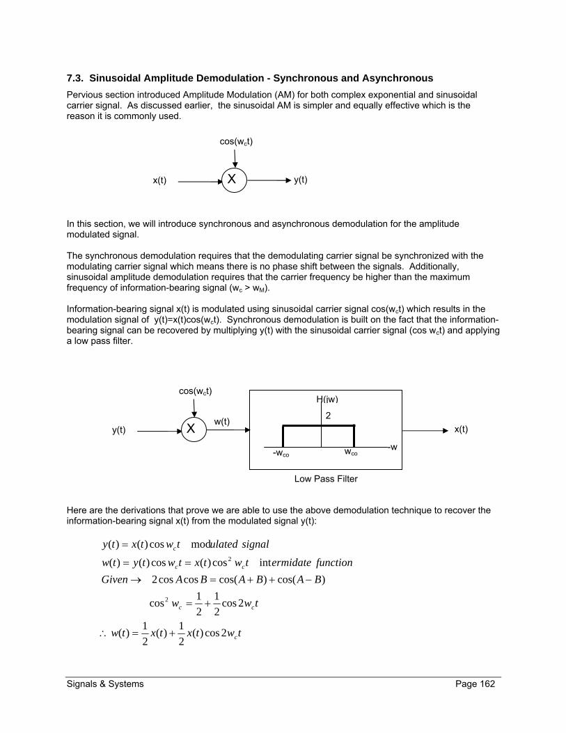
Signals & Systems Page 162
7.3. Sinusoidal Amplitude Demodulation - Synchronous and Asynchronous
Pervious section introduced Amplitude Modulation (AM) for both complex exponential and sinusoidal carrier signal. As discussed earlier, the sinusoidal AM is simpler and equally effective which is the reason it is commonly used.
In this section, we will introduce synchronous and asynchronous demodulation for the amplitude modulated signal. The synchronous demodulation requires that the demodulating carrier signal be synchronized with the modulating carrier signal which means there is no phase shift between the signals. Additionally, sinusoidal amplitude demodulation requires that the carrier frequency be higher than the maximum frequency of information-bearing signal (wc > wM). Information-bearing signal x(t) is modulated using sinusoidal carrier signal cos(wct) which results in the modulation signal of y(t)=x(t)cos(wct). Synchronous demodulation is built on the fact that the information-bearing signal can be recovered by multiplying y(t) with the sinusoidal carrier signal (cos wct) and applying a low pass filter.
Here are the derivations that prove we are able to use the above demodulation technique to recover the information-bearing signal x(t) from the modulated signal y(t):
twtxtxtw
tww
BABABAGiven
functionermidatetwtxtwtytw
signalulatedtwtxty
c
cc
cc
c
2cos)(2
1)(
2
1)(
2cos2
1
2
1cos
)cos()cos(coscos2
intcos)(cos)()(
modcos)()(
2
2
X
cos(wct)
w(t) y(t) x(t)
-wco wco -w
2
H(jw)
Low Pass Filter
X
cos(wct)
y(t) x(t)

Signals & Systems Page 163
We are able to extract x(t) by passing the intermediate function w(t) through a low pass filter with a gain of 2 and cut off frequency wc0 (wM wc0 <wc). Below are the frequency spectrum diagrams representing the steps of AM modulation and demodulation graphically:
C(jw)
w wc -wc
Y(jw)
w wc (-wc -wM) -wc (-wc + wM) (wc -wM) (wc + wM)
1/2
W(jw)
2wc (-2wc -wM) -2wc (-2wc + wM) (2wc -wM) (2wc + wM)
1/2
0
1/4 1/4
wM -wM
Low Pass Filter 2
X(jw)
1
0 wM -wM w

Signals & Systems Page 164
The following diagram provides a time-domain representation of the demodulation process:
The one challenge with synchronous demodulation is the requirement that the carrier signal at the receiver used to demodulate has to be synchronized with the signal used to modulate the signal at the transmitter (no phase shift). The asynchronous sinusoidal demodulation removes the requirement that the carrier signal at transmitting and receiving side have to have be in-phase (have the same phase). Asynchronous sinusoidal demodulation occurs when the demodulating signal w(t) is not in-phase with modulating signal y(t)
Where:
)()cos()cos()(
)()cos()(
)()cos()(
)cos()(
txtwtwtw
tytwtw
txtwty
twtc
cDcMcc
Dcc
Mcc
Mcc
X
cos(wct+Mc)
y(t) x(t) X
cos(wct+Dc)
w(t) xr(t) = cos(M-D)x(t)
-wco wco
2
H(jw)
Low Pass Filter
Transmitter & Modulator Receiver & Demodulator
X f(t)
cos(wct)
x(t)cos(wct)
Antenna
t t
x(t) cos2 (wct)
b) Carrier Signal, c(t) a) Modulated Signal, y(t)
Low Pass Filter (LPF)
f(t)cos2wct
f(t)cos(wct)
c) Input Signal, x(t)
x(t)

Signals & Systems Page 165
Given trigonometry relation )cos()cos(2
1coscos BABABA , w(t) can be rewritten as:
)()2cos(2
1)()cos(
2
1)( txtwtxtw McDccMcDc
In this situation, we can attempt to recover information-bearing signal x(t) from the modulated signal y(t) by only using the envelop (Peaks):
The two conditions required for this type of demodulation are: 1) x(t) must be positive 2) Carrier frequency wc is much higher than the maximum signal frequency, wM An example of modulator/demodulate system used to implement the asynchronous demodulation is outlined below:
The demodulation using envelop detector requires “A” to be sufficiently large so that x(t) + A is always positive. Since K is the maximum amplitude of x(t) then in order for x(t) + A to be positive, A must be larger than K (A >K). The ratio of K/A is called the modulation index m (m=K/A). You may also see m expressed in percent and called percent modulation. For example the modulated signal y(t) shown below has m =K/A=2/3= 67% modulation:
X
cos(wct)
y(t) = (A+ x(t)) cos(wct) x(t) where |x(t)| < K
+
A
t
y(t) x(t)
Envelop
Envelop

Signals & Systems Page 166
In order to derive a close approximation to the x(t), we can utilize the following low pass circuit:
An advantage of asynchronous modulation-demodulation over synchronous approach is that it does not need synchronized carriers at the modulation and demodulation. Disadvantage is that it requires the transmitter to transmit higher power since x(t) must be positive and A>K. Although it adds cost to the transmitter, it reduces the cost of the receivers. For example in the case of an AM radio, this is a desirable trade off, since there is only one transmitter station but many receivers.
R C
+ y(t) -
+ Approximation of x(t) -
Time Constant =1/RC must be significantly smaller than maximum x(t) period (TM = 2/wM) and larger than carrier period (Tc = 2/wc) TC<< <<TM
t
y(t)
A = 6
K = 4
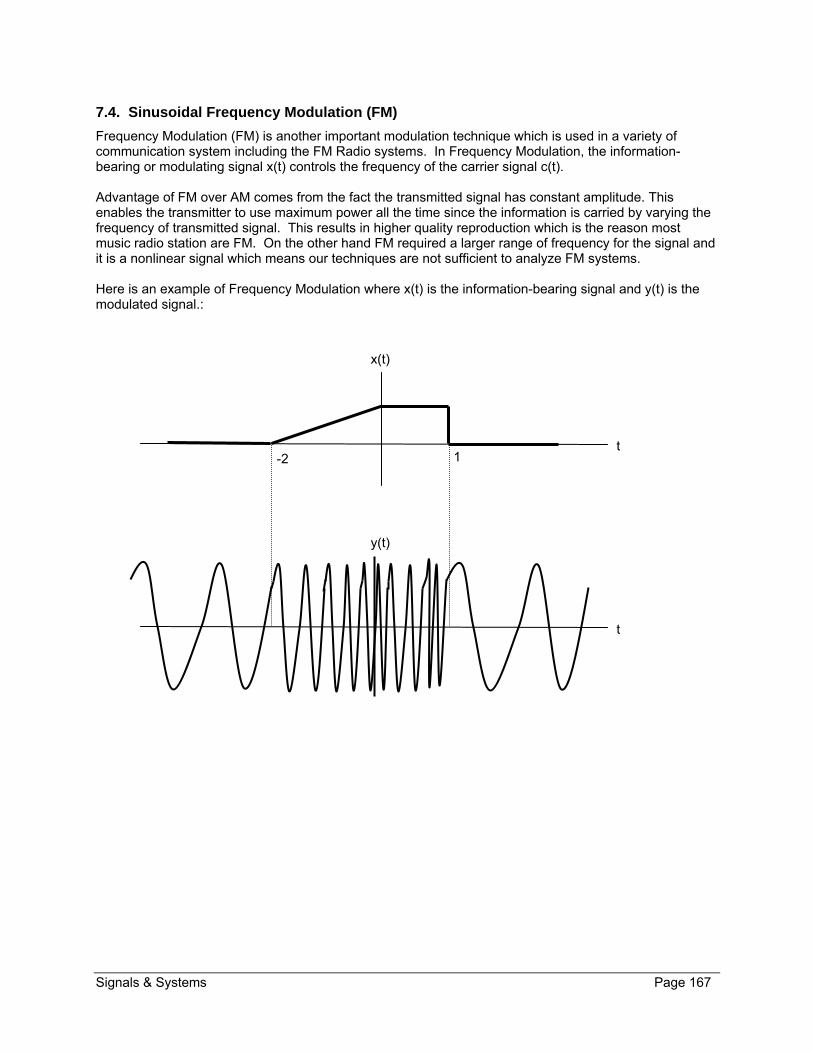
Signals & Systems Page 167
7.4. Sinusoidal Frequency Modulation (FM)
Frequency Modulation (FM) is another important modulation technique which is used in a variety of communication system including the FM Radio systems. In Frequency Modulation, the information-bearing or modulating signal x(t) controls the frequency of the carrier signal c(t). Advantage of FM over AM comes from the fact the transmitted signal has constant amplitude. This enables the transmitter to use maximum power all the time since the information is carried by varying the frequency of transmitted signal. This results in higher quality reproduction which is the reason most music radio station are FM. On the other hand FM required a larger range of frequency for the signal and it is a nonlinear signal which means our techniques are not sufficient to analyze FM systems. Here is an example of Frequency Modulation where x(t) is the information-bearing signal and y(t) is the modulated signal.:
t
x(t)
1-2
t
y(t)

Signals & Systems Page 168
7.5. Frequency-Division and Time-Division Multiplexing
In addition to using the modulation (shifting signal frequency) for matching the optimal frequency range of the selected channel, the modulation/demodulation technique may be used to transmit many signals on the same channel. This is accomplished by allocating each signal different parts of the frequency spectrum. This technique is referred to as Frequency-Division Multiplexing (FDM). Below is a system diagram for modulation and demodulation required for Frequency-Division Multiplexing:
The key requirement is that the signal carrier frequencies be far enough from each other so that frequency spectrum signals do not overlap. Below is an example of n signals being Frequency-Division Multiplexed onto a single channel signal as shown by the following frequency spectrum of the signals:
Another way to share the channel is Time-Division Multiplexing (TDM) which means each signal is given a defined period of time to use the channel. In other word, the channel is shared over time and at any given time there is only one signal being transmitted through the channel.
-wM1 wM1 w
x1(jw)
-wMn wMn w
xn(jw)
. . .
Y(jw)
wc1 -wc1 wcn -wcn
. . . . . .
X x1(t)
Cos(wc1t)
y1(t)
X
Cos(wcnt)
Yn(t) xn(t)
+. . .
Band pass filter
Low pass filter X
Cos(wc1t)
x1(t)
.
.
.
Band pass filter
Low pass filter X
Cos(wcnt)
xn(t)
y(t)
w

Signals & Systems Page 169
7.6. Common Modulation Techniques
Analog Modulation
o AM Amplitude modulation (AM) is a technique used modulate analog signal by changing the amplitude of the carrier signal.
o FM Frequency modulation (FM) is a technique used modulate analog signal by changing the frequency of the carrier signal.
o PM Phase modulation (FM) is a technique used modulate analog signal by changing the phase of the carrier signal.
Digital Modulation
o ASK
Amplitude-shift keying (ASK) represents digital data as changes in amplitude of carrier signal.
o FSK Frequency-shift keying (FSK) represents digital data as changes in Frequency of carrier signal.
o CPM Continuous phase modulation (CPM) is a form of digital data modulation.
Digital Data Transmission Support Encodings
o NRZI
Non-Return-to-Zero-Inverted (NRZI) is a method of mapping a binary signal to a physical signal for transmission. The two level NRZI signal has a transition at a clock boundary if the bit being transmitted is a logical 1, and does not have a transition if the bit being transmitted is a logical 0.

Signals & Systems Page 170
7.7. Additional Resources
Oppenheim, A. Signals & Systems (1997) Prentice Hall Chapter 8.
Lathi, B. Modern Digital & Analog Communication Systems (1998) Oxford University Press
Chapter 4.
Stremler, F. Introduction to Communication Systems (1990) Addison-Wesley Publishing Company Chapt 5,6 and 7.

Signals & Systems Page 171
7.8. Problems
Refer to www.EngrCS.com or online course page for complete solved and unsolved problem set.

Signals & Systems Page 172
Chapter 8. Laplace Transform
Key Concepts and Overview Laplace Transform
Inverse Laplace Transform
Region Of Convergence (ROC)
Laplace Transform Properties
Application of Laplace Transform to LTI Systems
Additional Resources

Signals & Systems Page 173
8.1. Laplace Transform “X(s) = Lx(t)”
The continuous-time Fourier Transform has proven to be an effective tool in analysis of LTI system behavior across a broad range of signals. Fourier Transform provides representation of signals as linear combinations of complex exponential signals in the form: est where s=jw “pure imaginary” This chapter introduces Laplace Transform which is an extension of continuous Fourier Transform. The Laplace Transform extends the definition of s such that: s = σ + jw “s is a complex number” In addition to covering a broader range of signals, Laplace Transforms enables analysis of system that may only be stable in a some regions. Later in this chapter, Laplace transform will be used in analysis of such LTI systems. Throughout this chapter, we will discuss bilateral Laplace transform. There is a special case Laplace transform which is called Unilateral Laplace transform where t ≤ 0- is assume to be zero. Unilateral Laplace transform is typically used for LTI systems with zero initial conditions. In this chapter, it will be demonstrated that there exist many similarities between Fourier transform and Laplace transform operation. Therefore we can leverage our knowledge of Fourier transform and take advantage of Laplace transform’s additional benefits and flexibility. The following relation is a restatement of result of earlier work on time-domain to frequency domain transforms:
dtethsHwhereesHty stst )()()()(
where s=jw (pure imaginary) Frequency response H(s) is the Fourier Transform of impulse response h(t).
The above relationship may be generalized by stating that s is a complex variable (s=σ+jw). The change in the value of s to a complex numbers instead of pure imaginary yields:
dtetxsX st)()( Referred to as the Laplace Transform equation (s=σ+jw)
Laplace Transform is Represented by )()( sXtx L or Lx(t) = X(s)
It can be seen from the following equation that when s=jw, Laplace transform changes to a Fourier transform:
jws
jwt sXdtetxtxFjwX
)()()()(
Another observation is the relationship between the Fourier Transform and Laplace Transform when (s=σ+jw). The following derivation demonstrates the relationship:
)()()()()( )( tjwtttjw etxFdteetxdtetxtxLSX
or

Signals & Systems Page 174
Lx(t) = Fx(t)e-at Example – Laplace Transform derivation
Example 1 – Find the Laplace transform of the signal x(t) = [2e-at + 5e-bt]u(t). Solution:
))((
)52(752)(
52)
]52]52[)(
52)(52)()(
0)(
0)(
0
)jw(
0
)jw(
0
)()(
0
sbsa
bas
sbsasX
esb
esa
sX
dtedtedteesX
dteeedtetueedtetxsX
tsbtsa
tbtatsbtsa
stbtatstbtatst
Another consideration is the convergence which requires the integrals to have values less than infinity:
asbb
asaa
requireseConvergenc
dteedteedtedtesX jwttbjwttatbta
Re0
Re0
:
52]52)(0
)t(
0
)t(
0
)jw(
0
)jw(
Latter in this section the topic of Region of Convergence (ROC) will be covered in more detail.
Example 2 - Find the Laplace transform for the signal x(t) = 5 sin(3t) e-2t u(t) Solution: Student Exercise
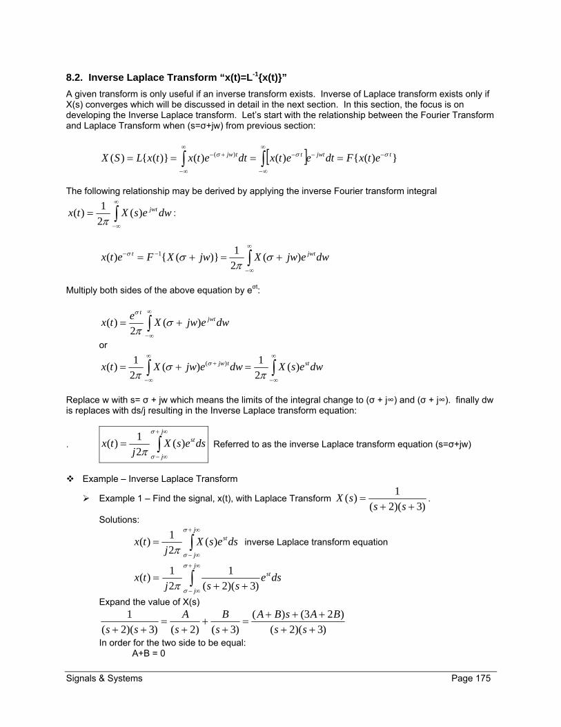
Signals & Systems Page 175
8.2. Inverse Laplace Transform “x(t)=L-1x(t)”
A given transform is only useful if an inverse transform exists. Inverse of Laplace transform exists only if X(s) converges which will be discussed in detail in the next section. In this section, the focus is on developing the Inverse Laplace transform. Let’s start with the relationship between the Fourier Transform and Laplace Transform when (s=σ+jw) from previous section:
)()()()()( )( tjwtttjw etxFdteetxdtetxtxLSX
The following relationship may be derived by applying the inverse Fourier transform integral
dwesXtx jwt)(2
1)(
:
dwejwXjwXFetx jwtt )(2
1)()( 1
Multiply both sides of the above equation by eσt:
dwejwXe
tx jwtt
)(2
)(
or
dwesXdwejwXtx sttjw )(2
1)(
2
1)( )(
Replace w with s= σ + jw which means the limits of the integral change to (σ + j∞) and (σ + j∞). finally dw is replaces with ds/j resulting in the Inverse Laplace transform equation:
.
j
j
stdsesXj
tx
)(
2
1)( Referred to as the inverse Laplace transform equation (s=σ+jw)
Example – Inverse Laplace Transform
Example 1 – Find the signal, x(t), with Laplace Transform )3)(2(
1)(
sssX .
Solutions:
j
j
stdsesXj
tx
)(
2
1)( inverse Laplace transform equation
j
j
stdsessj
tx
)3)(2(
1
2
1)(
Expand the value of X(s)
)3)(2(
)23()(
)3()2()3)(2(
1
ss
BAsBA
s
B
s
A
ss
In order for the two side to be equal: A+B = 0

Signals & Systems Page 176
3A+2B =1 Solve the system of two equation and two unknowns to find A=1 and B =-1, therefore:
j
j
j
j
ststj
j
st dsesj
dsesj
dsessj
tx
)3(
1
2
1
)2(
1
2
1
)3(
1
)2(
1
2
1)(
Need to make the power of est and the denominator the same by multiply/dividing powers of e:
2Re)()(
22)(
)3(
1
2)2(
1
2)(
)3(
1
2
1
)2(
1
2
1)(
32
)3(3
)2(2
)3(3
)2(2
3
3
2
2
sfortueetx
MISSINGSTEPS
ej
ee
j
etx
dsesj
edse
sj
etx
dsee
e
sjdse
e
e
sjtx
tt
j
j
tstj
j
tst
j
j
j
j
tst
tst
j
j
j
j
stt
tst
t
t
As it can been seen from the above example, we can find the inverse Laplace transform with the use of inverse Laplace transforms equation for a class of ration Laplace transforms of the form:
tsconsareakandAkwhereas
AsX
N
k k
k tan)(1
N
k
tak tueAtx k
1
)()( if ROC is Res >-ak
N
k
tak tueAtx k
1
)()( if ROC is Re s <-ak
Example 2 – Find the signal x(t) with Laplace transform 3212
2)(
2
sssX
Solution: Student Exercise

Signals & Systems Page 177
8.3. Region Of Convergence (ROC)
The Laplace Transform Region of Convergence (ROC) is the range of value of (s=σ + jw) where valid
Laplace transform
dtetxsX st)()( exists. For valid Laplace transform to exist, we only need to
show that the following inequality is true:
dtetx t|)(|
Typically, ROC is shown in a rectangular coordinate which is referred to as s-plane. The vertical axis (jw-axis) is the imaginary part of s (Ims=w) and horizontal axis (σ-axis)is the real part of s (Res= σ). The shaded area of the s-plane is the ROC. Below are two examples of ROC in s-planes:
In the case where the signal x(t) is a linear combination of real or complex exponential, its Laplace transform is rational. Which means, it is ratio of numerator over denominator in term of complex variable s:
)(
)()(
sD
sNsX
As simple example would be x(t) = 5e-4tu(t) + 2e-3tu(t). In this case x(t) is a linear combination of real exponential. Its Laplace transform is rational and can be calculated by:
sssX
es
es
dteesX
dteeedtetxsX
tstststs
stttst
3
5
4
2)(
3
5
4
2]25[)(
25)()(
0)3(
0)3(
0
)3()4(
0
34
Res, σ
Ims, jw
ROC
-2 Res, σ
Ims, jw
ROC
-4
a) ROC is Res < -2 b) ROC is Res > -4
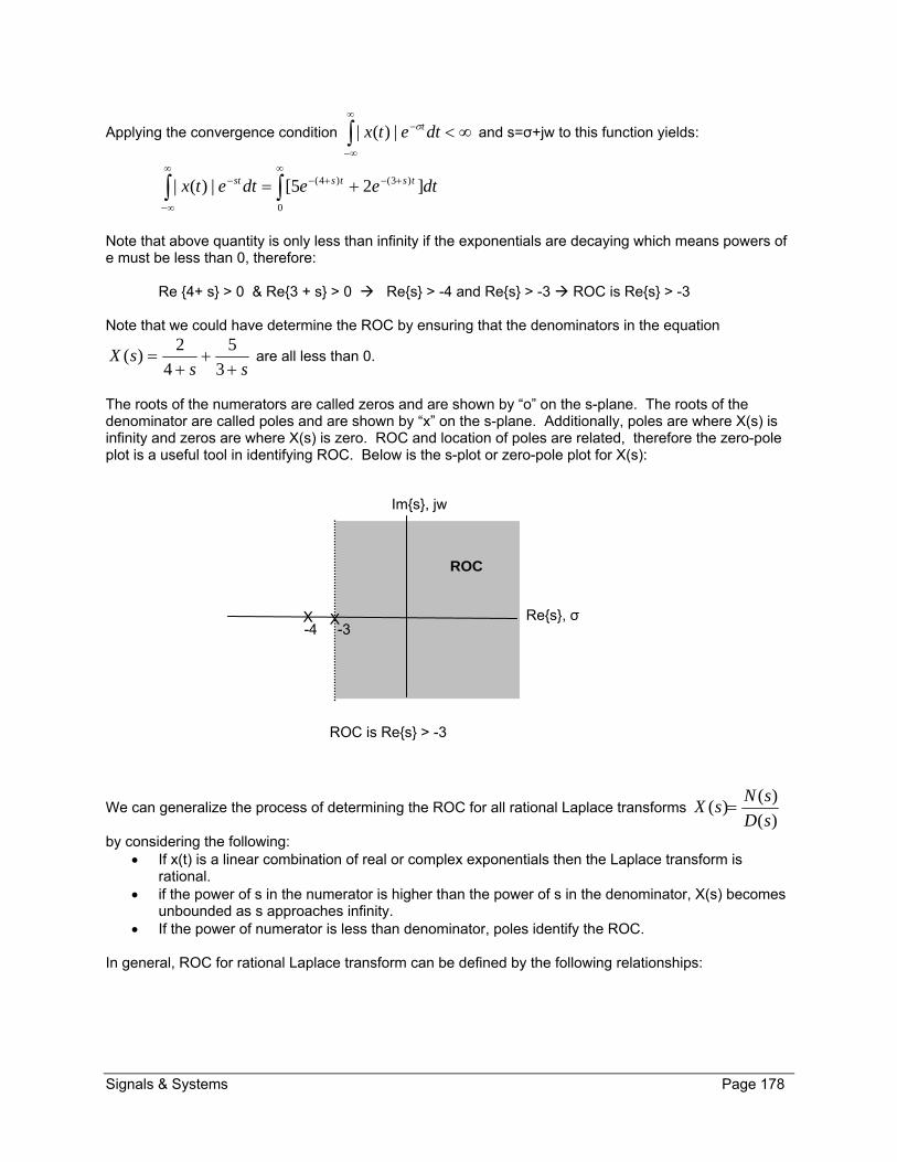
Signals & Systems Page 178
Applying the convergence condition
dtetx t|)(| and s=σ+jw to this function yields:
0
)3()4( ]25[|)(| dteedtetx tstsst
Note that above quantity is only less than infinity if the exponentials are decaying which means powers of e must be less than 0, therefore: Re 4+ s > 0 & Re3 + s > 0 Res > -4 and Res > -3 ROC is Res > -3 Note that we could have determine the ROC by ensuring that the denominators in the equation
sssX
3
5
4
2)( are all less than 0.
The roots of the numerators are called zeros and are shown by “o” on the s-plane. The roots of the denominator are called poles and are shown by “x” on the s-plane. Additionally, poles are where X(s) is infinity and zeros are where X(s) is zero. ROC and location of poles are related, therefore the zero-pole plot is a useful tool in identifying ROC. Below is the s-plot or zero-pole plot for X(s):
We can generalize the process of determining the ROC for all rational Laplace transforms )(
)()(
sD
sNsX
by considering the following: If x(t) is a linear combination of real or complex exponentials then the Laplace transform is
rational. if the power of s in the numerator is higher than the power of s in the denominator, X(s) becomes
unbounded as s approaches infinity. If the power of numerator is less than denominator, poles identify the ROC.
In general, ROC for rational Laplace transform can be defined by the following relationships:
Res, σ
Ims, jw
ROC
-4 -3
ROC is Res > -3
X X

Signals & Systems Page 179
i i
i
as
A
sD
sNsX
)(
)()( ROC is where:
Res > - Reai when Ai > 0 Res < - Reai when Ai < 0 Example – ROC for Rational Laplace Transform
Example 1 - Find the Laplace transform with its ROC for the function x(t) = e-7tu(t) + e-3tu(-t). Solution:
It is understood that Lx(t)=X(s)= 3
1
7
1
ss
ROC for first term Rs > -7 ROC for second term Rs < -3 Therefore the ROC for X(s) is -7 < Rs < -3 The following s-plan shows the ROC (shaded area):
Example 1 – Find the Laplace transform with its ROC for the function
x(t) = [e-4t + e-2t cos(5t)] u(t). Solutions: x(t) = [e-4t + ½ e-2t ej5t + e-j5t ] u(t) = [e-4t + ½ e(-2 + j5)t + ½ e(-2 - j5)t]u(t)
252ReRe52
2/1
252ReRe52
2/1
4Re4
1
)52(
2/1
)52(
2/1
4
1)(
2
1
2
1)()(
0
)52()52(4
jsROCjs
jsROCjs
sROCs
jsjsssX
dteeeedtetxsX sttjtjtst
Res, σ
Ims, jw
ROC
-7 -3
ROC is Res > -3
XX
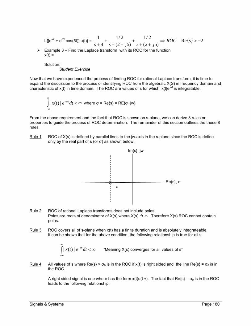
Signals & Systems Page 180
L[e-4t + e-2t cos(5t)] u(t) = 2Re)52(
2/1
)52(
2/1
4
1
sROC
jsjss
Example 3 – Find the Laplace transform with its ROC for the function x(t) = Solution: Student Exercise
Now that we have experienced the process of finding ROC for rational Laplace transform, it is time to expand the discussion to the process of identifying ROC from the algebraic X(S) in frequency domain and characteristic of x(t) in time domain. The ROC are values of s for which |x(t|e-t is integratable:
dtetx t|)(| where σ = Res = REσ+jw
From the above requirement and the fact that ROC is shown on s-plane, we can derive 8 rules or properties to guide the process of ROC determination. The remainder of this section outlines the these 8 rules: Rule 1 ROC of X(s) is defined by parallel lines to the jw-axis in the s-plane since the ROC is define
only by the real part of s (or σ) as shown below:
Rule 2 ROC of rational Laplace transforms does not include poles.
Poles are roots of denominator of X(s) where X(s) . Therefore X(s) ROC cannot contain poles.
Rule 3 ROC covers all of s-plane when x(t) has a finite duration and is absolutely integrateable. It can be shown that for the above condition, the following relationship is true for all s:
dtetx t|)(| ”Meaning X(s) converges for all values of s”
Rule 4 All values of s where Res > σ0 is in the ROC if x(t) is right sided and the line Res = σ0 is in
the ROC. A right sided signal is one where has the form x(t)u(t-). The fact that Res = σ0 is in the ROC leads to the following relationship:
Res, σ
Ims, jw
-aX
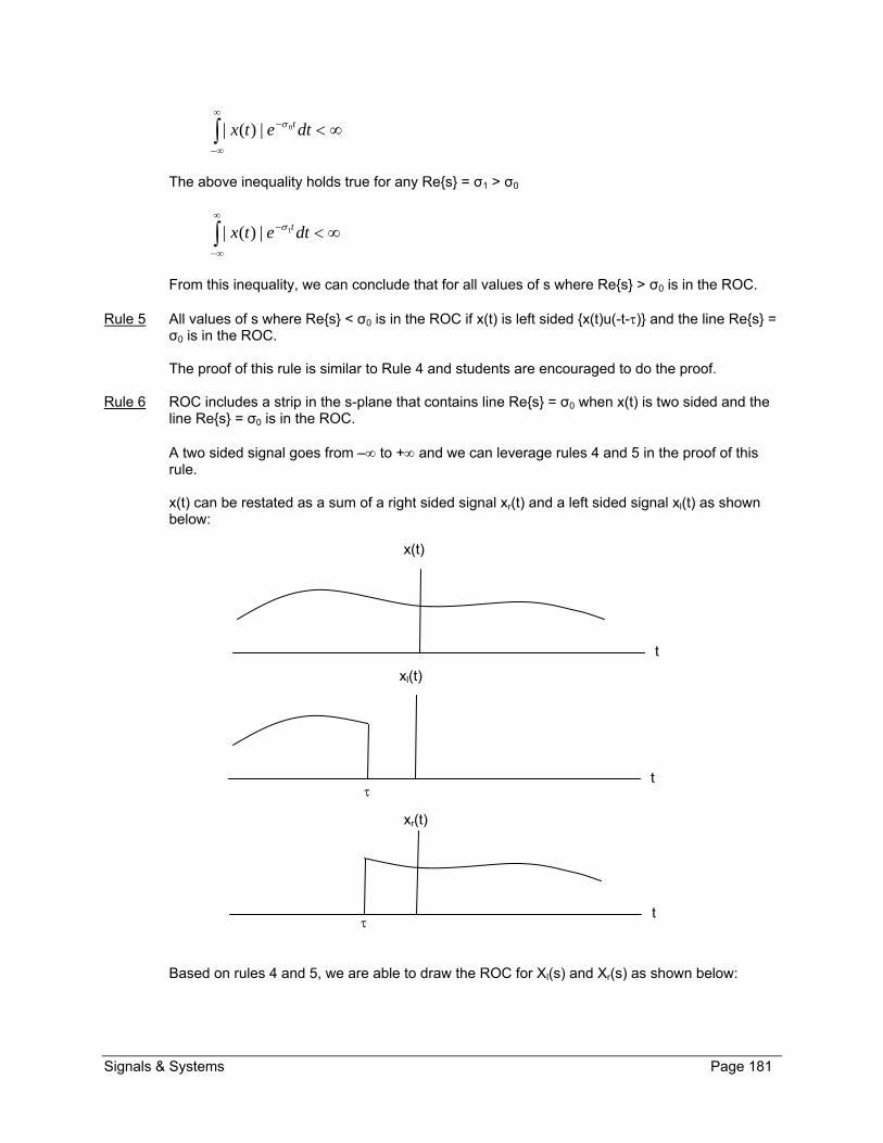
Signals & Systems Page 181
dtetx t0|)(|
The above inequality holds true for any Res = σ1 > σ0
dtetx t1|)(|
From this inequality, we can conclude that for all values of s where Res > σ0 is in the ROC.
Rule 5 All values of s where Res < σ0 is in the ROC if x(t) is left sided x(t)u(-t-) and the line Res = σ0 is in the ROC. The proof of this rule is similar to Rule 4 and students are encouraged to do the proof.
Rule 6 ROC includes a strip in the s-plane that contains line Res = σ0 when x(t) is two sided and the line Res = σ0 is in the ROC. A two sided signal goes from – to + and we can leverage rules 4 and 5 in the proof of this rule. x(t) can be restated as a sum of a right sided signal xr(t) and a left sided signal xl(t) as shown below:
Based on rules 4 and 5, we are able to draw the ROC for Xl(s) and Xr(s) as shown below:
x(t)
t
xl(t)
t
xr(t)
t
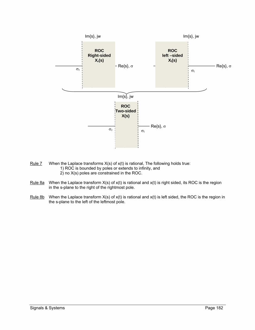
Signals & Systems Page 182
Rule 7 When the Laplace transforms X(s) of x(t) is rational, The following holds true: 1) ROC is bounded by poles or extends to infinity, and 2) no X(s) poles are constrained in the ROC.
Rule 8a When the Laplace transform X(s) of x(t) is rational and x(t) is right sided, its ROC is the region in the s-plane to the right of the rightmost pole.
Rule 8b When the Laplace transform X(s) of x(t) is rational and x(t) is left sided, the ROC is the region in the s-plane to the left of the leftmost pole.
Ims, jw
Res, r
ROC Right-sided
Xr(s)
Ims, jw
Res, l
ROC left –sided
Xl(s)
Ims, jw
Res, r
ROC Two-sided
X(s)
l

Signals & Systems Page 183
8.4. Laplace Transform Properties
Laplace Transform has properties that are similar to the Fourier Transform. The following table contains the most common properties of Laplace Transform:
Property
Time-Domain x(t), x1(t), x2(t)
Laplace s-Domain X(s), X1(s), X2(s)
ROC R, R1, R2
Linearity ax1(t) + bx2(t) aX1(s) + bX2(s) At least R1 ∩ R2 Time shifting x(t - t0) )(0 sXe t
R
Shifting in the s-Domain )(0 txe ts
X(s – s0) Shifted R ”s is in R if (s – s0) is in R”
Time scaling x(at)
)(||
1
a
sX
a
Scaled R ”s is in R if s/a is in R”
Convolution x1(t) * x2(t) X1(s)X2(s) At least R1 ∩ R2 Conjunction x*(t) X*(s*) R
Differentiation in t
n
n
dt
txd )(
snX(s) At least R
Differentiation in s (-1)n tn x(t)
n
n
ds
sXd )(
R
Integration in t
)()(
t
dx )(1
sXs
At Least R ∩ [Res > 0]
Note: ∩ “Intersection of sets” resulting set includes only the common elements of the two sets. U “Union of sets” resulting set includes all the elements of both sets. One may proof these properties by apply the Laplace transform or Laplace inverse transform equations.
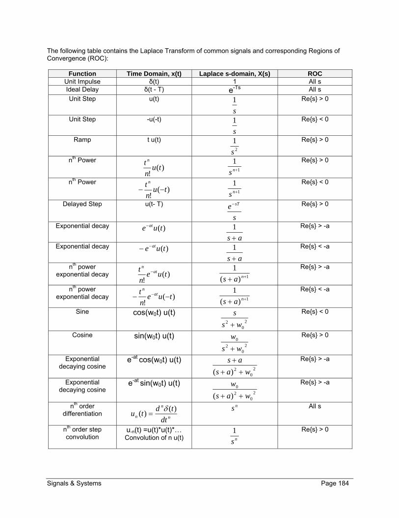
Signals & Systems Page 184
The following table contains the Laplace Transform of common signals and corresponding Regions of Convergence (ROC):
Function Time Domain, x(t) Laplace s-domain, X(s) ROC Unit Impulse δ(t) 1 All s Ideal Delay δ(t - T) e-Ts All s
Unit Step u(t)
s
1
Res > 0
Unit Step -u(-t)
s
1
Res < 0
Ramp t u(t) 2
1
s
Res > 0
nth Power )(
!tu
n
t n
1
1ns
Res > 0
nth Power )(
!tu
n
t n
1
1ns
Res < 0
Delayed Step u(t- T)
s
e sT
Res > 0
Exponential decay )(tue at
as 1
Res > -a
Exponential decay )(tue at
as 1
Res < -a
nth power exponential decay )(
!tue
n
t atn
1)(
1 nas
Res > -a
nth power exponential decay )(
!tue
n
t atn
1)(
1 nas
Res < -a
Sine cos(w0t) u(t) 2
02 ws
s
Res < 0
Cosine sin(w0t) u(t) 2
02
0
ws
w
Res > 0
Exponential decaying cosine
e-at cos(w0t) u(t) 2
02)( was
as
Res > -a
Exponential decaying cosine
e-at sin(w0t) u(t) 2
02
0
)( was
w
Res > -a
nth order differentiation
n
n
n dt
tdtu
)()(
ns All s
nth order step convolution
u-n(t) =u(t)*u(t)*… Convolution of n u(t) ns
1
Res > 0
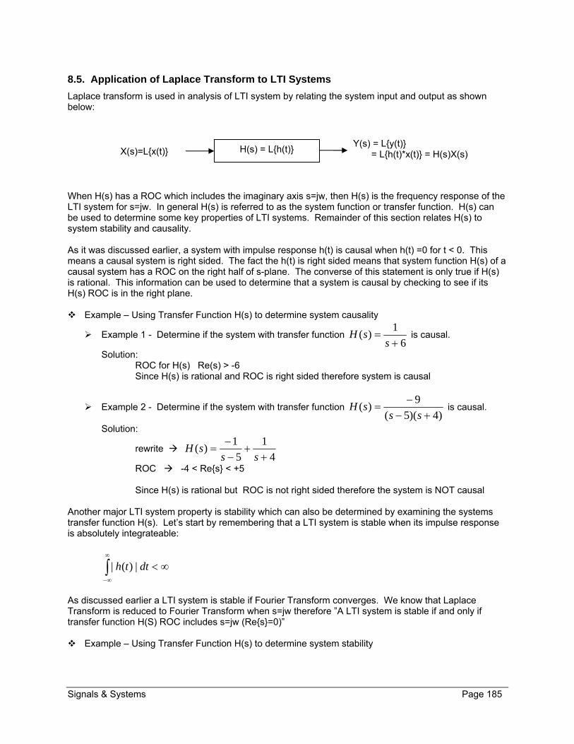
Signals & Systems Page 185
8.5. Application of Laplace Transform to LTI Systems
Laplace transform is used in analysis of LTI system by relating the system input and output as shown below:
When H(s) has a ROC which includes the imaginary axis s=jw, then H(s) is the frequency response of the LTI system for s=jw. In general H(s) is referred to as the system function or transfer function. H(s) can be used to determine some key properties of LTI systems. Remainder of this section relates H(s) to system stability and causality. As it was discussed earlier, a system with impulse response h(t) is causal when h(t) =0 for t < 0. This means a causal system is right sided. The fact the h(t) is right sided means that system function H(s) of a causal system has a ROC on the right half of s-plane. The converse of this statement is only true if H(s) is rational. This information can be used to determine that a system is causal by checking to see if its H(s) ROC is in the right plane. Example – Using Transfer Function H(s) to determine system causality
Example 1 - Determine if the system with transfer function 6
1)(
ssH is causal.
Solution: ROC for H(s) Re(s) > -6 Since H(s) is rational and ROC is right sided therefore system is causal
Example 2 - Determine if the system with transfer function )4)(5(
9)(
ss
sH is causal.
Solution:
rewrite 4
1
5
1)(
ss
sH
ROC -4 < Res < +5 Since H(s) is rational but ROC is not right sided therefore the system is NOT causal
Another major LTI system property is stability which can also be determined by examining the systems transfer function H(s). Let’s start by remembering that a LTI system is stable when its impulse response is absolutely integrateable:
dtth |)(|
As discussed earlier a LTI system is stable if Fourier Transform converges. We know that Laplace Transform is reduced to Fourier Transform when s=jw therefore ”A LTI system is stable if and only if transfer function H(S) ROC includes s=jw (Res=0)” Example – Using Transfer Function H(s) to determine system stability
H(s) = Lh(t) X(s)=Lx(t) Y(s) = Ly(t) = Lh(t)*x(t) = H(s)X(s)

Signals & Systems Page 186
Example 1 - Determine if the system with transfer function 2
1)(
ssH is stable.
Solution: ROC for H(s) Re(s) > 2 Since ROC does not include s=jw or Res=0, the system is not stable.
Example 2 - Determine if the system with transfer function )4)(5(
9)(
ss
sH is stable.
Solution:
rewrite 4
1
5
1)(
ss
sH
ROC -4 < Res < +5 Since ROC contain s=jw or Res=0, the system is stable.

Signals & Systems Page 187
8.6. Additional Resources
Oppenheim, A. Signals & Systems (1997) Prentice Hall
Chapter 9. Nilsson, J. Electrical Circuits. (2004) Pearson.
Chapter 12 and 13.

Signals & Systems Page 188
8.7. Problems
Refer to www.EngrCS.com or online course page for complete solved and unsolved problem set.

Signals & Systems Page 189
Chapter 9. Z-Transform
Key Concepts and Overview Z-Transform
Inverse Z-Transform
Region Of Convergence (ROC)
Z-Transform Properties
Application of Z-Transform in LTI Systems
Additional Resources
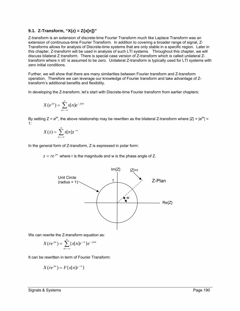
Signals & Systems Page 190
9.1. Z-Transform, “X(z) = Zx[n]”
Z-transform is an extension of discrete-time Fourier Transform much like Laplace Transform was an extension of continuous-time Fourier Transform. In addition to covering a broader range of signal, Z-Transforms allows for analysis of Discrete-time systems that are only stable in a specific region. Later in this chapter, Z-transform will be used in analysis of such LTI systems. Throughout this chapter, we will discuss bilateral Z transform. There is special case version of Z-transform which is called unilateral Z-transform where n ≤0- is assumed to be zero. Unilateral Z-transform is typically used for LTI systems with zero initial conditions. Further, we will show that there are many similarities between Fourier transform and Z-transform operation. Therefore we can leverage our knowledge of Fourier transform and take advantage of Z-transform’s additional benefits and flexibility. In developing the Z-transform, let’s start with Discrete-time Fourier transform from earlier chapters:
n
jwnjw enxeX ][)(
By setting Z = ejw, the above relationship may be rewritten as the bilateral Z-transform where |Z| = |ejw| = 1:
n
nznxzX ][)(
In the general form of Z-transform, Z is expressed in polar form:
jwrez where r is the magnitude and w is the phase angle of Z.
We can rewrite the Z-transform equation as:
n
jwnnjw ernxreX ][)(
It can be rewritten in term of Fourier Transform:
][)( njw rnxFreX
ReZ w
|Z|=r
Unit Circle (radius = 1) Z-Plan 1
ImZ

Signals & Systems Page 191
Z-transform can be characterized based on value of “r” as shown below:
Decaying when r>1 Growing when r<1
For r=1 z-transform is reduced to Fourier transform ][)()( nxFeXzX jw
ez jw

Signals & Systems Page 192
9.2. Inverse Z-Transform, “x[n] = Z-1X(z)”
TBC

Signals & Systems Page 193
9.3. Region Of Convergence (ROC)
Z-transform Region Of Convergence (ROC) is define by using the unit circuit introduced earlier:
For X(z) to converge, Fourier transform of x[n]r-n must converge and ROC on Z-Plan are value of z for which X(z) converges. If ROC contains the circle then Fourier transform of x[n] also converges.
Example 1. Find ROC for x[n]=anu[n] Apply the Z-transform analysis equation
0
1 )(][][)(n
n
n
nn
n
n azznuaznxzX
For X(z) to converge we require
0
1 ||n
naz which means |az-1| < 1 or |z|>|a|
Applying the finite sum we get: az
z
azzX
11
1)( when |z|>|a|
The requirement |z|>|a| defines the Region of Convergence (ROC) for X(Z) as the shaded area in the following pole-zero plot when 0<|a|<1:
Imaginary
Real w
Z=ejw
Unit Circle
Z-Plan
1
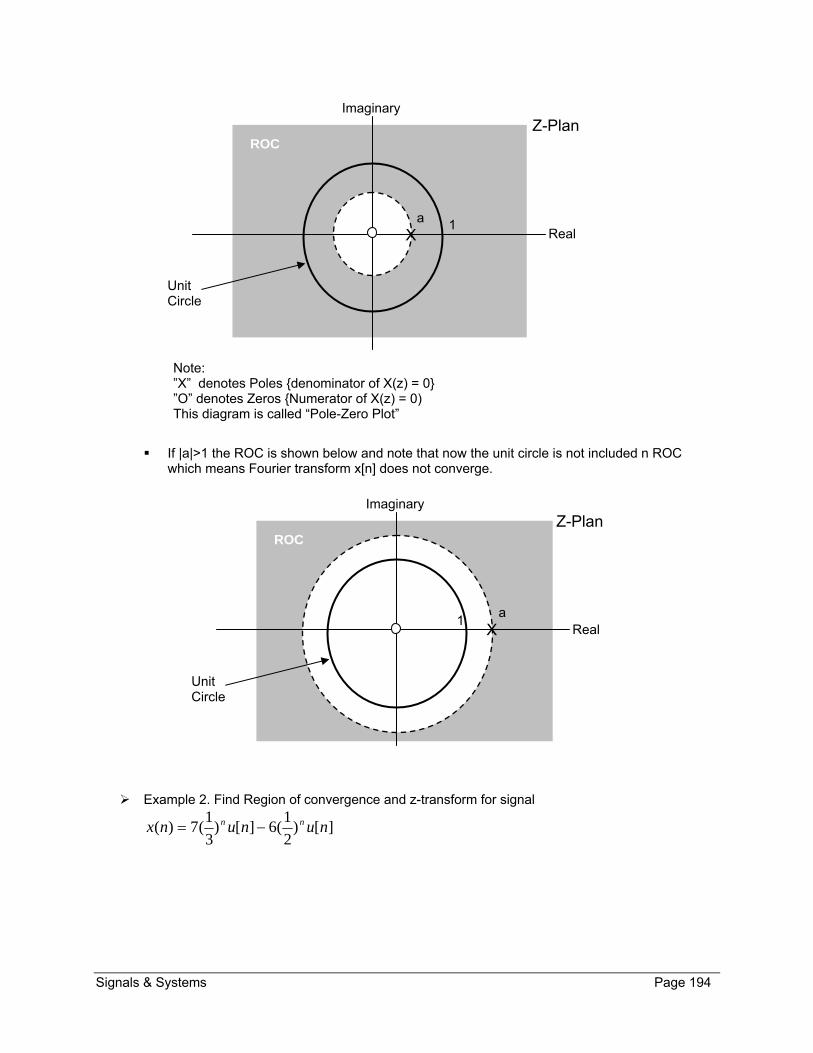
Signals & Systems Page 194
If |a|>1 the ROC is shown below and note that now the unit circle is not included n ROC
which means Fourier transform x[n] does not converge.
Example 2. Find Region of convergence and z-transform for signal
][)2
1(6][)
3
1(7)( nununx nn
Imaginary
Real
Z-Plan
1 a
ROC
Unit Circle
X
Imaginary
Real
Z-Plan
1 a
ROC
Unit Circle
X
Note: ”X” denotes Poles denominator of X(z) = 0 ”O” denotes Zeros Numerator of X(z) = 0) This diagram is called “Pole-Zero Plot”

Signals & Systems Page 195
0 0
11 )2
1(6)
3
1(7)(
][)2
1(6][)
3
1(7)(
][)2
1(6][)
3
1(7][)(
n n
nn
n n
nnnn
n
nnn
n
n
zzzX
znuznuzX
znunuznxzX
First term requires |(1/3)z-1|<1 |z|>1/3 second term requires |(1/2)z-1|<1 |z|>1/2 Therefore X(z) converges when |z|>1/2 and applying infinite sum relationship we get z-transform:
2/1||
2
11
6
3
11
7)(
11
zwherezz
zX
combining the fraction we get a rational function:
2/1||)
2
1)(
3
1(
)2
3(
)(
zwhere
zz
zzzX
Two Zeros: 0 & 3/2 Two poles: 1/3 & 1/2 Pole-zero plot and ROC are shown below:
Example 4. Find Region of convergence and z-transform for sequence
][)4
sin()3
1()( nunnx n
Imaginary
Real
Z-Plan
1
ROC
Unit Circle
X X 1/3 1/2 3/2
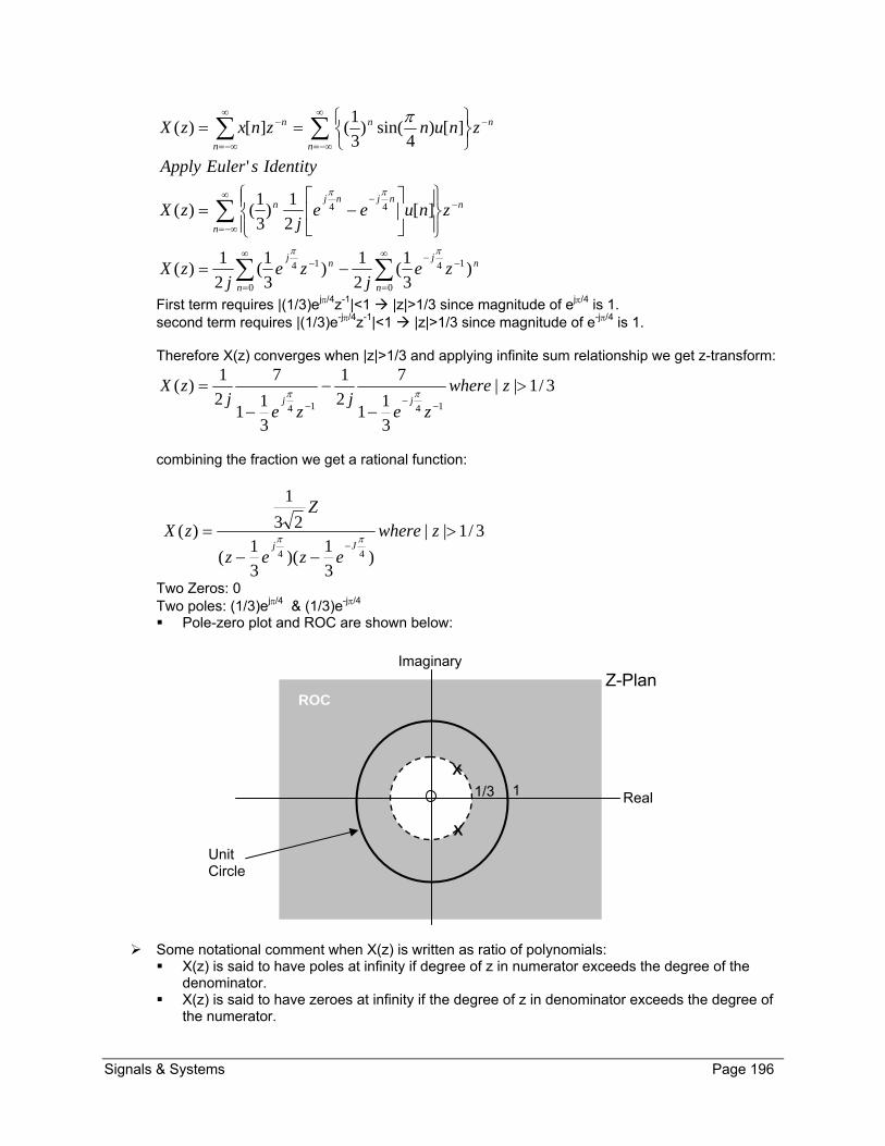
Signals & Systems Page 196
0
14
0
14
44
)3
1(
2
1)
3
1(
2
1)(
][2
1)
3
1()(
'
][)4
sin()3
1(][)(
n
nj
n
nj
n
nnjnj
n
n
nn
n
n
zej
zej
zX
znueej
zX
IdentitysEulerApply
znunznxzX
First term requires |(1/3)ej/4z-1|<1 |z|>1/3 since magnitude of ej/4 is 1. second term requires |(1/3)e-j/4z-1|<1 |z|>1/3 since magnitude of e-j/4 is 1. Therefore X(z) converges when |z|>1/3 and applying infinite sum relationship we get z-transform:
3/1||
3
11
7
2
1
3
11
7
2
1)(
1414
zwhere
zej
zej
zXjj
combining the fraction we get a rational function:
3/1||
)3
1)(
3
1(
23
1
)(44
zwhere
ezez
ZzX
Jj
Two Zeros: 0 Two poles: (1/3)ej/4 & (1/3)e-j/4 Pole-zero plot and ROC are shown below:
Some notational comment when X(z) is written as ratio of polynomials:
X(z) is said to have poles at infinity if degree of z in numerator exceeds the degree of the denominator.
X(z) is said to have zeroes at infinity if the degree of z in denominator exceeds the degree of the numerator.
Imaginary
Real
Z-Plan
1
ROC
Unit Circle
X
X
1/3
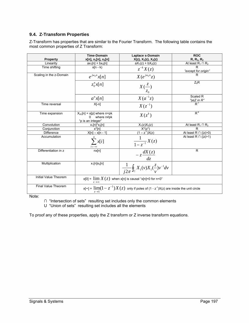
Signals & Systems Page 197
9.4. Z-Transform Properties
Z-Transform has properties that are similar to the Fourier Transform. The following table contains the most common properties of Z Transform:
Property
Time-Domain x[n], x1[n], x2[n]
Laplace s-Domain X(z), X1(z), X2(z)
ROC R, R1, R2
Linearity ax1[n] + bx2[n] aX1(z) + bX2(z) At least R1 ∩ R2 Time shifting x[n - k) )(zXz k
R
”except for origin”Scaling in the z-Domain ][0 nxe njw
)( 0 zeX njw
R
][0 nxzn )(
0z
zX
Z0R
][nxan )( 1zaX
Scaled R ”|a|Z in R”
Time reversal X[-n] )( 1zX R-1
Time expansion X(k)[n] = x[p] where n=pk 0 where n≠pk “p is an integer”
)( kzX R-k
Convolution x1[n]*x2[n] X1(z)X2(z) At least R1 ∩ R2 Conjunction x*[n] X*(z*) R Difference X[n] – x[n - 1] (1 – z-1)X(z) At least R ∩ (|z|>0)
Accumulation
n
i
ix ][ )(1
11 zX
z
At least R ∩ (|z|>1)
Differentiation in z nx[n]
dz
zdXz
)(
R
Multiplication x1[n]x2[n]
dvvv
zXvX
j C
111 )()(
2
1
Initial Value Theorem x[0] = )(lim zXz
when x[n] is causal “x[n]=0 for n<0”
Final Value Theorem x[∞] = )()1(lim 1
1zXz
z
only if poles of (1 - z-1)X(z) are inside the unit circle
Note: ∩ “Intersection of sets” resulting set includes only the common elements U “Union of sets” resulting set includes all the elements To proof any of these properties, apply the Z transform or Z inverse transform equations.

Signals & Systems Page 198
The following table contains the Z-Transform of common signals and corresponding Regions of Convergence (ROC):
Function Time Domain, x(t) Laplace s-domain, X(s) ROC Unit Impulse δ[n] 1 All z Ideal Delay δ[n – n0] 0nz Z ≠ 0
Unit Step u[n] 11
1 z
|z| > 1
Unit Step -u[-n-1] 11
1 z
|z| < 1
Ramp nu[n]
21
1
)1(
z
z
|z| > 1
Ramp -nu[-n-1]
21
1
)1(
z
z
|z| < 1
nth Power ][nuan 11
1 az
|z| > |a|
nth Power ]1[ nuan 11
1 az
|z| < |a|
nth Power ][nunan 21
1
)1(
az
az
|z| > |a|
nth Power ]1[ nunan 21
1
)1(
az
az
|z| < |a|
Cosine [cosw0n]u[n]
210
10
]cos2[1
][cos1
zzw
zw
|z| > 1
Sine [sinw0n]u[n]
210
10
]sin2[1
][sin
zzw
zw
|z| > 1
nth Power Cosine rn[cosw0n]u[n]
2210
10
]cos2[1
]cos[
zrzwr
zwr
|z| > r
nth Power Sine rn[sinw0n]u[n]
2210
10
]sin2[1
]sin[
zrzwr
zwr
|z| > r

Signals & Systems Page 199
9.5. Application of Z-Transform in LTI Systems
Z-transformation applies to discrete-time linear time-Invariant system with impulse response h[n], the system response y[n] to x[n] as shown below:
h[n]
n
nznhzH ][)( x[n] y[n] = H(z)x[n]
Signals & Systems Page 200
9.6. Additional Resources
Oppenheim, A. Signals & Systems (1997) Prentice Hall
Chapter10

Signals & Systems Page 201
9.7. Problems
Refer to www.EngrCS.com or online course page for complete solved and unsolved problem set.

Signals & Systems Page 202
Appendix A. Additional Resources
Additional resources are available at the author’s website http://www.EngrCS.com/
Future Enhancements Add study questions, practical problems. Expand Laplace and Z transform chapters.
![Continuous Time Signals & Systems: Part Ieeweb.poly.edu/~yao/EE3054/Chap9.1_9.5.pdf · Signals and Systems Continuous Time Signals & Systems: Part I Yao Wang ... DISCRETE-TIME: x[n]](https://img.dokumen.tips/doc/110x75/5b8493d97f8b9ae0498c7b9d/continuous-time-signals-systems-part-yaoee3054chap9195pdf-signals-and.jpg)


![Fourier Representation for Continuous Time Signals · · 2016-07-07Fourier Representation for Continuous Time Signals ... • Discrete-time signal x[n] ... Sketches for different](https://img.dokumen.tips/doc/110x75/5aeca2ec7f8b9a3b2e8f695a/fourier-representation-for-continuous-time-signals-representation-for-continuous.jpg)