Shortwave aerosol radiative forcing over cloud-free oceans

from Terra:

2. Seasonal and global distributions

Jianglong Zhang,1,2 and Sundar A. ChristopherDepartment of Atmospheric Sciences, University of Alabama, Huntsville, Alabama, USA

Lorraine A. Remer and Yoram J. KaufmanNASA Goddard Space Flight Center Data Center, Greenbelt, Maryland, USA

Received 12 May 2004; revised 18 August 2004; accepted 1 December 2004; published 9 March 2005.

[1] Using 10 months of collocated Clouds and the Earth’s Radiant Energy System(CERES) scanner and Moderate Resolution Imaging Spectroradiometer (MODIS) aerosoland cloud data from Terra, we provide estimates of the shortwave aerosol direct radiativeforcing (SWARF) and its uncertainties over the cloud-free global oceans. Newlydeveloped aerosol angular distribution models (ADMs) (Zhang et al., 2005), specificallyfor different sea surface conditions and aerosol types, are used for inverting the CERESobserved radiances to shortwave fluxes while accounting for the effect of aerosol opticalproperties on the anisotropy of the top of atmosphere (TOA) shortwave radiationfields. The spatial and seasonal distributions of SWARF are presented, and the MODISretrieved aerosol optical depth (t0.55) and the independently derived SWARF show ahigh degree of correlation and can be estimated using the equation SWARF = 0.05 �74.6 t0.55 + 18.2 t0.55

2 W m�2 (t0.55 < 0.8). The instantaneous TOA SWARF from Terraoverpass time is �6.4 ± 2.6 W m�2 for cloud-free oceans. Accounting for samplebiases and diurnal averaging, we estimate the SWARF over cloud-free oceans to be �5.3 ±1.7 W m�2, consistent with previous studies. Our study is an independent measurement-based assessment of cloud-free aerosol radiative forcing that could be used as a validationtool for numerical modeling studies.

Citation: Zhang, J., S. A. Christopher, L. A. Remer, and Y. J. Kaufman (2005), Shortwave aerosol radiative forcing over cloud-free

oceans from Terra: 2. Seasonal and global distributions, J. Geophys. Res., 110, D10S24, doi:10.1029/2004JD005009.

1. Introduction

[2] Owing to their significance in climate change studies[Intergovernmental Panel on Climate Change (IPCC),2001], aerosols and their radiative effects have been studiedthrough various methods [e.g., Hansen et al., 1998;Haywood et al., 1999]. Commonly used approaches tostudy the effect of aerosols on climate include either simpleradiative transfer equations [e.g., Penner et al., 1994] orcomplex general circulation models [Hansen et al., 1998].However, satellite observations have also been used to studythe shortwave aerosol radiative forcing (SWARF) overcloud-free conditions [Loeb and Kato, 2002; Christopherand Zhang, 2002, 2004]. In these studies, satellite broad-band observations from either the Earth Radiation BudgetExperiment (ERBE) or Clouds and the Earth’s RadiantEnergy System (CERES) are classified into three groupsof data including ‘‘clear,’’ ‘‘cloud-free aerosol skies’’ and

‘‘cloudy skies’’ through the use of additional multispectralsatellite observations. The SWARF over cloud-free skies isthen derived by removing the clear sky component from thetop of atmosphere (TOA) fluxes. Since the CERES has alarge footprint on the order of 20 km at nadir on Terra,additional finer spatial resolution satellite observations areneeded to obtain aerosol and cloud properties within theCERES footprint.[3] Using a similar approach from the Visible Infrared

Scanner (VIRS) and CERES data on board the TropicalRainfall Measuring Mission (TRMM), Christopher et al.[2000] studied the SWARF over both land and ocean. Loeband Kato [2002] extended this study using nine months ofcollocated VIRS and CERES data, and reported diurnallyaveraged SWARF of �4.6 W m�2 over the tropical oceans.However, the VIRS was not designed for aerosol studiesand has several limitations including limited number ofspectral channels, limited spatial coverage (only 37N–37S),and coarse spatial resolution of 2 km when compared withother current imagers such as Moderate Resolution ImagingSpectroradiometer (MODIS).[4] The recently launched Terra and Aqua satellites

provide an excellent opportunity for studying both aerosoland SWARF using space observations. Onboard these

JOURNAL OF GEOPHYSICAL RESEARCH, VOL. 110, D10S24, doi:10.1029/2004JD005009, 2005

1Now at Naval Research Laboratory, Monterey, California, USA.2Visiting scientist from University Corporation for Atmospheric

Research, Boulder, Colorado, USA.

Copyright 2005 by the American Geophysical Union.0148-0227/05/2004JD005009$09.00

D10S24 1 of 10

satellites, the Moderate Resolution Imaging Spectroradiom-eter (MODIS) has a total of 36 channels with improvedspatial, spectral and radiometric resolutions when comparedwith previous imagers [King et al., 1992]. A major goal ofMODIS is to characterize the spatial distribution of aerosolsand clouds and their optical properties. Over global oceans,the MODIS is used to retrieve aerosol optical depth andaerosol particle size information and have been intensivelyvalidated against ground and insitu measurements [e.g.,Remer et al., 2002]. Also on board Terra, the CERES,which is a broadband instrument, can be used to obtainTOA outgoing shortwave and longwave fluxes. TheMODIS cloud and aerosol information and the CERESTOA fluxes have been merged together to form the CERESSingle Scanner Footprint (SSF) data [Loeb and Kato, 2002],which can be used to examine the effect of aerosols on theEarth-atmosphere system. Since the CERES does not ob-serve SW fluxes directly, Angular Dependence Models(ADMs) are used for inverting the observed radiance toTOA flux for a given scene [Wielicki et al., 1996]. Using tenmonths of MODIS and CERES data from Terra, newaerosol ADMs have been developed specifically for satelliteSWARF studies and is an improvement over the previousERBE and TRMM ADMs [Zhang et al., 2005].[5] In this paper, we examine the SWARF over global

cloud-free oceans and the seasonal and regional distribu-tions of SWARF are also presented. Different from ourprevious efforts [Christopher and Zhang, 2002], the effectsof solar zenith angle, clear-sky bias, diurnal averaging andthe ratio of fine mode to total aerosol optical depth on thesatellite-derived SWARF are investigated.

2. Data Sets

[6] The details of the CERES and MODIS data sets arediscussed in detail in the work of Zhang et al. [2005] andonly a brief summary is provided here. We used ten months(November 2000 to August 2001) of the CERES SSFproduct that contains the point spread function weightedaerosol and cloud properties [Loeb et al., 2003] includingthe aerosol optical depth and the ratio (h) of fine aerosol tototal aerosol optical depth at 0.47, 0.55 and 0.67 mm[Kaufman et al., 2005; Remer et al., 2002]. The MODISretrieved aerosol optical properties at 0.55 mm (t0.55) areused in this study and recent studies show that the MODISretrieved aerosol optical depth values (t0.55) are within theexpected uncertainties of ±0.03 ± 0.05 t0.55 over the globaloceans [Remer et al., 2002]. In this study, only CERESobservations over cloud-free oceans are used and we requirethe CERES pixels to be at least 99.9% cloud-free asdetermined by MODIS data.

3. Methods and Results

[7] In a companion paper [Zhang et al., 2005], wedescribe the angular models that were developed for con-verting the CERES measured radiances to TOA fluxes forcloud-free pixels. The new aerosol ADMs are built asfunctions of SSM/I wind speed, the ratio of fine modeAOT to total AOT (h), and the MODIS aerosol opticalthickness. In previous studies [e.g., Loeb and Kato, 2002;Christopher and Zhang, 2002], over cloud-free oceans,

there was only one set of ADMs available and aerosoldarkening effect over glint regions and aerosol brighteningeffect over nonglint regions are not considered and there-fore, the derived SWARF could be overestimated [Zhang etal., 2005]. For the TRMM ADMs, only one aerosol model(maritime tropical aerosol model) for correcting the effectsof aerosols on the angular distribution pattern of TOA SWradiation fields is assumed, and therefore the SWARF couldbe underestimated. In this study, we compare the SWARFusing ERBE, TRMM, and Terra ADMS over cloud-freeoceans and examine the seasonal and spatial distribution ofSWARF from the newly constructed ADMs.[8] The SWARF is defined as the difference in the SW

flux observed without (Fclr) and with (Faero) the presence ofaerosols [e.g., Ackerman and Chung, 1992; Christopherand Zhang, 2002] where Fclr is ‘‘clear-sky’’ flux thatrepresents TOA CERES fluxes in cloud and aerosol-freeconditions and Faero is the observed cloud-free CERESTOA SW flux in the presence of aerosols. Both Fclr andFaero are computed for every 2 � 2 degree latitude,longitude bins and due to the significant increase in pixelsize as a function of scan angle, only the CERES pixels thathave viewing zenith angle less than 60� and solar zenithangle less than 60� are used. The SWARF is derived bysubtracting the Fclr of a 2 � 2 degree bin from the binaveraged cloud-free CERES flux.[9] To obtain SWARF, the TOA SW fluxes in aerosol and

cloud-free conditions are needed where Fclr is defined as theSW flux when MODIS t0.55 = 0. However, it is not possibleto have observed scenes that have zero aerosol loading.Therefore, in this study, the Fclr is computed using the twosteps. First, the seasonal mean Fclr values are constructed asfunctions of solar zenith angle (qo) and near surface windspeed. Owing to uncertainties in MODIS aerosol retrievals atvery low optical depths [e.g.,Remer et al., 2002], it is difficultto isolate CERES pixels with zero t0.55. Therefore we assumethat for observations with t0.55 < 0.2, CERES fluxes andMODIS t0.55 have a linear relationship [Christopher andZhang, 2002] and for each qo and wind speed bin (ten qoand four wind speed bins), the linear regression relation(equation (1)) is computed using all cloud-free CERES pixelsthat have t0.55 < 0.2.

SW flux ¼ Fclr þ slope*t0:55 ð1Þ

[10] The Fclr is obtained by extrapolating the regressionrelation back to zero t0.55. Using this approach, lookuptables of Fclr and the slope of SW flux versus t0.55 areestablished as functions of wind speed and qo. Therefore, fora given CERES observation, the Fclr can be obtained usingthe predetermined LUTs.[11] Averaging over all solar zenith angle bins and all wind

speed bins, the Fclr values are 70.4, 72.0 and 74.6 W m�2 forthe Northern Hemisphere summer (June–July–August),spring (March–April–May), and winter (November–December–January–February) seasons, respectively. Owingto variations in oceanic and atmospheric conditions such aswater vapor, Fclr also shows local variations. To account forthese local variations, a correction factor is computed locally.For each bin, the mean SW flux, t0.55, qo and wind speed forCERES pixels that have t0.55 < 0.2 are computed for eachseason. The mean qo and wind speed are used as indices to

D10S24 ZHANG ET AL.: SEASONAL AND GLOBAL DISTRIBUTIONS

2 of 10

D10S24

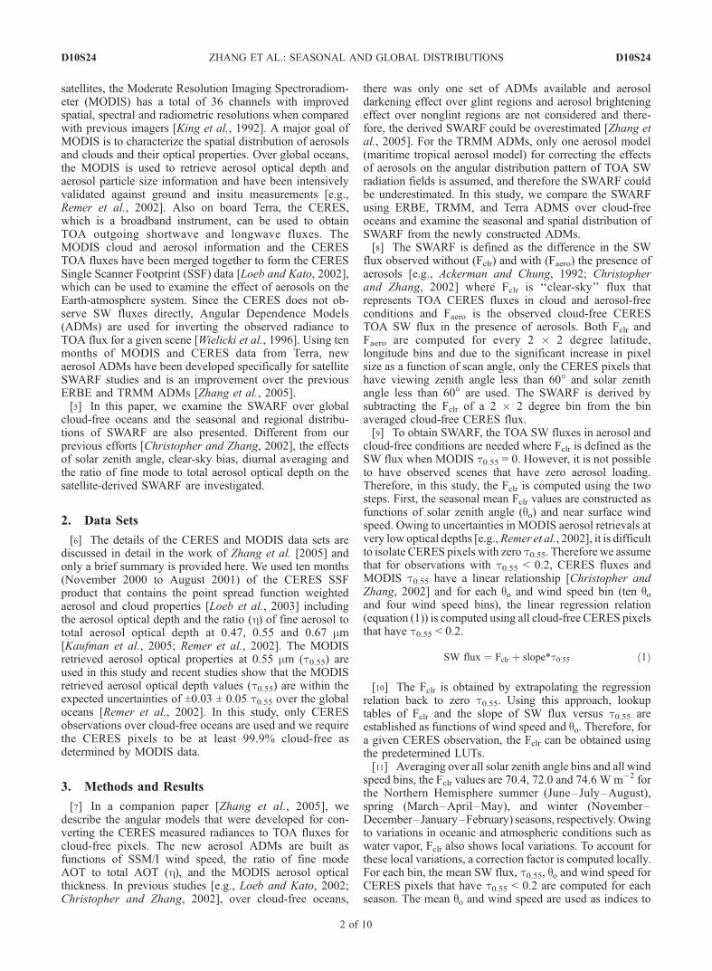
retrieve both Fclr and the slope of the regression relation fromthe predetermined LUTs. Using the retrieved regressionrelation, a new flux value is derived by inputting the averagedt0.55 value. The difference between the averaged and derivedfluxes (DF) is assumed to be from local variations and Fclr istherefore adjusted by adding the correction term DF that arethe order of 1.71, 1.34 and 1.67Wm�2 for the winter, spring,and summer seasons, respectively.[12] Figures 1a–1f show the global distribution of

MODIS t0.55 and CERES-derived SWARF over cloud-freeoceans for winter, spring, and summer seasons. Thesevalues are called instantaneous because they are derivedfrom the time of the satellite overpass. The geographicaldistribution of t0.55 and CERES-derived SWARF are con-sistent, and regions with high t0.55 are associated withregions of high SWARF. For example, in winter, both high

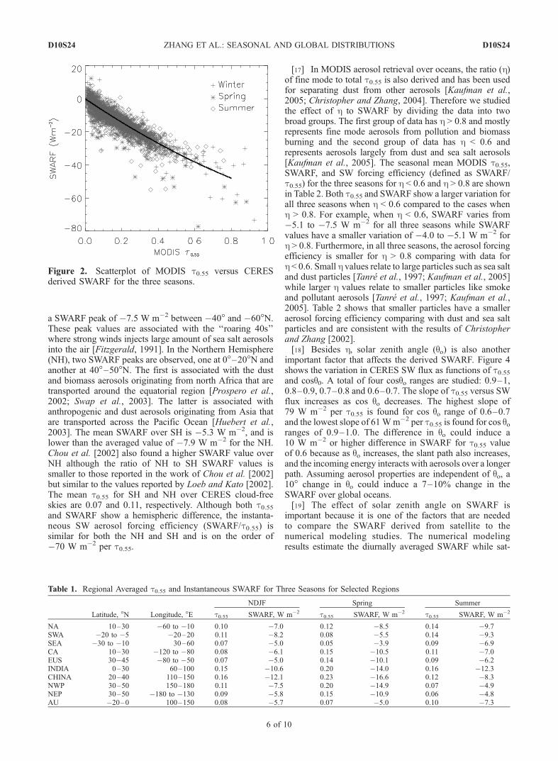
aerosol loading and high SWARF are observed over thewest coast of Africa, the Indian Ocean and the east coast ofAsia. Figure 2 shows the scatterplot of t0.55 versus SWARFfor the three seasons. The scatterplots for the three seasonsshow a similar pattern when t0.55 < 0.6, while for t0.55 >0.6, the SWARF values from spring and winter seasons arehigher than that of the summer season. The aerosol forcingefficiency, that is defined as the mean SWARF of the seasondivided by the mean t0.55 of the season, are: �72, �73,and �70 W m�2 per t0.55 for the winter, spring andsummer seasons, respectively. Also shown in Figure 2 bythe thick black line is a second-order polynomial fit for allthree seasons where SWARF = 0.05 � 74.6t0.55 +18.2t0.55

2 W m�2. The slope of t0.55 versus SWARF in thisstudy is higher than previously reported in the work ofChristopher and Zhang, [2002] where SWARF was studied

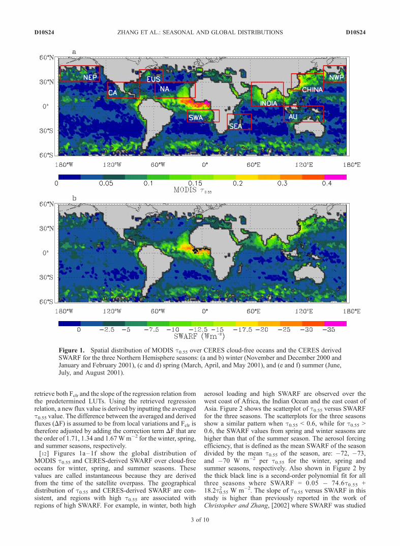
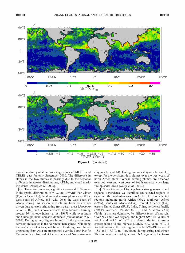
Figure 1. Spatial distribution of MODIS t0.55 over CERES cloud-free oceans and the CERES derivedSWARF for the three Northern Hemisphere seasons: (a and b) winter (November and December 2000 andJanuary and February 2001), (c and d) spring (March, April, and May 2001), and (e and f) summer (June,July, and August 2001).

D10S24 ZHANG ET AL.: SEASONAL AND GLOBAL DISTRIBUTIONS

3 of 10

D10S24

over cloud-free global oceans using collocated MODIS andCERES data for only September 2000. The difference inslopes in the two studies is possibly due to the seasonaldifference in aerosol distributions, ADMs, and cloud mask-ing issues [Zhang et al., 2005].[13] There are, however, significant seasonal differences

in the spatial distribution of t0.55, and SWARF. For winter(Figures 1a and 1b), the dominant aerosol plumes are off thewest coast of Africa, and Asia. Over the west coast ofAfrica, during this season, aerosols are from both wind-driven dust aerosols originating from desert areas [Prosperoet al., 2002], and smoke aerosols from biomass burningaround 10� latitude [Husar et al., 1997] while over Indiaand China, pollutant aerosols dominate [Ramanathan et al.,2001]. During spring (Figures 1c and 1d), the predominantaerosols are located in the Northern Hemisphere (NH) alongthe west coast of Africa, and India. The strong dust plumesoriginating from Asia are transported over the North PacificOcean and are observed at the west coast of North America

(Figures 1c and 1d). During summer (Figures 1e and 1f),except for the persistent dust plumes over the west coast ofnorth Africa, thick biomass burning plumes are observedover both east and west coast of South America when largefire episodes occur [Swap et al., 2003].[14] Since the aerosol forcing has a strong seasonal and

regional dependence we identified ten selected regions toexamine the instantaneous SWARF. The ten selectedregions including north Africa (NA), southwest Africa(SWA), southeast Africa (SEA), Central America (CA),eastern United States (EUS), India, China, northwest Pacific(NWP), northeast Pacific (NEP), and Australia (AU)(Table 1) that are dominated by different types of aerosols.Over NA and SWA regions, the highest SWARF values of�9.7 and �9.3 W m�2 are found during summercorresponding to the highest MODIS t0.55 value of 0.14for both regions. For NA region, smaller SWARF values of�8.5 and �7.0 W m�2 are found during spring and winter.The dominant aerosol type over NA region is the trans-

Figure 1. (continued)

D10S24 ZHANG ET AL.: SEASONAL AND GLOBAL DISTRIBUTIONS

4 of 10

D10S24

ported dust aerosol originating from the Saharan deserts[e.g., Prospero et al., 2002]. The high SWARF values overNA region for all three regions indicate the persistent dustSW cooling effect over that region. For SWA region, duringspring, no significant aerosol plumes are apparent inFigure 1, and SWARF is as low as �5.5 W m�2. Duringwinter, due to the biomass burning activities in South Africathat typically starts around August and lasts until November[Swap et al., 2003], the SWARF in SWA region increases to�8.2 W m�2.[15] Over India and China, the mean instantaneous

SWARF reaches high values of �14.0 and �16.6 W m�2

during spring. High SWARF values are also found duringsummer and remain high through the winter for both of theregions. The fraction of fine mode to the total aerosoloptical depth, as indicated by h is high for India where finemode aerosol dominates the spring and winter seasons whilecoarse mode aerosols such as dust aerosols transported fromNA region, dominate the summer season. Over China, the

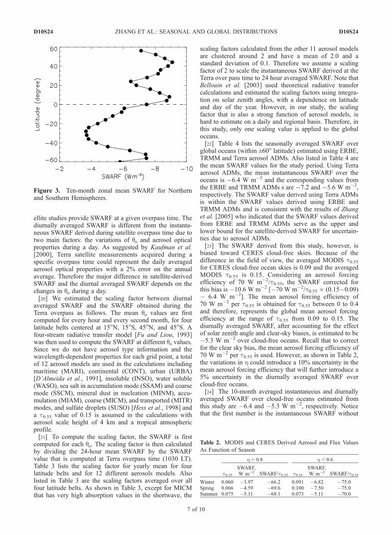
fine mode aerosols dominate at all seasons, although duringspring the h value is the lowest. Similarly, the highestSWARF values of �14.9 and �10.9 W m�2 are also foundover NWP and NEP regions for the same period. It isinteresting to note that SWARF values are gradually re-duced from source to NWP and NEP, which possiblyindicates the direction of aerosol transport. In other twoseasons, both NWP and NEP regions have low SWARFvalues. Also, during spring, both CA and EUS have hight0.55 and SWARF values compared with other seasons.Over CA, the SWARF values are �7.0, �10.5 and�6.1 W m�2 for summer, spring and winter, respectively.The high SWARF and t0.55 values during spring areassociated with biomass burning events during that seasonover Central America [Christopher et al., 2000].[16] Figure 3 shows the zonal mean SWARF over cloud-

free oceans calculated from the time of the satellite over-pass. In the Southern Hemisphere (SH), the minimumSWARF values are found near �20� to �40� latitude with

Figure 1. (continued)

D10S24 ZHANG ET AL.: SEASONAL AND GLOBAL DISTRIBUTIONS

5 of 10

D10S24

a SWARF peak of �7.5 W m�2 between �40� and �60�N.These peak values are associated with the ‘‘roaring 40s’’where strong winds injects large amount of sea salt aerosolsinto the air [Fitzgerald, 1991]. In the Northern Hemisphere(NH), two SWARF peaks are observed, one at 0�–20�N andanother at 40�–50�N. The first is associated with the dustand biomass aerosols originating from north Africa that aretransported around the equatorial region [Prospero et al.,2002; Swap et al., 2003]. The latter is associated withanthropogenic and dust aerosols originating from Asia thatare transported across the Pacific Ocean [Huebert et al.,2003]. The mean SWARF over SH is �5.3 W m�2, and islower than the averaged value of �7.9 W m�2 for the NH.Chou et al. [2002] also found a higher SWARF value overNH although the ratio of NH to SH SWARF values issmaller to those reported in the work of Chou et al. [2002]but similar to the values reported by Loeb and Kato [2002].The mean t0.55 for SH and NH over CERES cloud-freeskies are 0.07 and 0.11, respectively. Although both t0.55and SWARF show a hemispheric difference, the instanta-neous SW aerosol forcing efficiency (SWARF/t0.55) issimilar for both the NH and SH and is on the order of�70 W m�2 per t0.55.

[17] In MODIS aerosol retrieval over oceans, the ratio (h)of fine mode to total t0.55 is also derived and has been usedfor separating dust from other aerosols [Kaufman et al.,2005; Christopher and Zhang, 2004]. Therefore we studiedthe effect of h to SWARF by dividing the data into twobroad groups. The first group of data has h > 0.8 and mostlyrepresents fine mode aerosols from pollution and biomassburning and the second group of data has h < 0.6 andrepresents aerosols largely from dust and sea salt aerosols[Kaufman et al., 2005]. The seasonal mean MODIS t0.55,SWARF, and SW forcing efficiency (defined as SWARF/t0.55) for the three seasons for h < 0.6 and h > 0.8 are shownin Table 2. Both t0.55 and SWARF show a larger variation forall three seasons when h < 0.6 compared to the cases whenh > 0.8. For example, when h < 0.6, SWARF varies from�5.1 to �7.5 W m�2 for all three seasons while SWARFvalues have a smaller variation of �4.0 to �5.1 W m�2 forh > 0.8. Furthermore, in all three seasons, the aerosol forcingefficiency is smaller for h > 0.8 comparing with data forh < 0.6. Small h values relate to large particles such as sea saltand dust particles [Tanre et al., 1997; Kaufman et al., 2005]while larger h values relate to smaller particles like smokeand pollutant aerosols [Tanre et al., 1997; Kaufman et al.,2005]. Table 2 shows that smaller particles have a smalleraerosol forcing efficiency comparing with dust and sea saltparticles and are consistent with the results of Christopherand Zhang [2002].[18] Besides h, solar zenith angle (qo) is also another

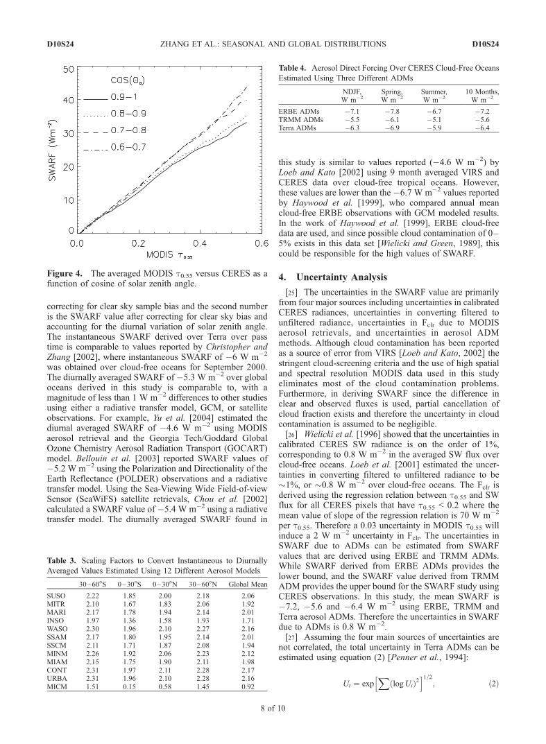
important factor that affects the derived SWARF. Figure 4shows the variation in CERES SW flux as functions of t0.55and cosq0. A total of four cosqo ranges are studied: 0.9–1,0.8–0.9, 0.7–0.8 and 0.6–0.7. The slope of t0.55 versus SWflux increases as cos qo decreases. The highest slope of79 W m�2 per t0.55 is found for cos qo range of 0.6–0.7and the lowest slope of 61Wm�2 per t0.55 is found for cos qoranges of 0.9–1.0. The difference in qo could induce a10 W m�2 or higher difference in SWARF for t0.55 valueof 0.6 because as qo increases, the slant path also increases,and the incoming energy interacts with aerosols over a longerpath. Assuming aerosol properties are independent of qo, a10� change in qo could induce a 7–10% change in theSWARF over global oceans.[19] The effect of solar zenith angle on SWARF is

important because it is one of the factors that are neededto compare the SWARF derived from satellite to thenumerical modeling studies. The numerical modelingresults estimate the diurnally averaged SWARF while sat-

Table 1. Regional Averaged t0.55 and Instantaneous SWARF for Three Seasons for Selected Regions

Latitude, �N Longitude, �E

NDJF Spring Summer

t0.55 SWARF, W m�2 t0.55 SWARF, W m�2 t0.55 SWARF, W m�2

NA 10–30 �60 to �10 0.10 �7.0 0.12 �8.5 0.14 �9.7SWA �20 to �5 �20–20 0.11 �8.2 0.08 �5.5 0.14 �9.3SEA �30 to �10 30–60 0.07 �5.0 0.05 �3.9 0.09 �6.9CA 10–30 �120 to �80 0.08 �6.1 0.15 �10.5 0.11 �7.0EUS 30�45 �80 to �50 0.07 �5.0 0.14 �10.1 0.09 �6.2INDIA 0–30 60–100 0.15 �10.6 0.20 �14.0 0.16 �12.3CHINA 20–40 110–150 0.16 �12.1 0.23 �16.6 0.12 �8.3NWP 30–50 150–180 0.11 �7.5 0.20 �14.9 0.07 �4.9NEP 30–50 �180 to �130 0.09 �5.8 0.15 �10.9 0.06 �4.8AU �20–0 100–150 0.08 �5.7 0.07 �5.0 0.10 �7.3

Figure 2. Scatterplot of MODIS t0.55 versus CERESderived SWARF for the three seasons.

D10S24 ZHANG ET AL.: SEASONAL AND GLOBAL DISTRIBUTIONS

6 of 10

D10S24

ellite studies provide SWARF at a given overpass time. Thediurnally averaged SWARF is different from the instanta-neous SWARF derived during satellite overpass time due totwo main factors: the variations of qo and aerosol opticalproperties during a day. As suggested by Kaufman et al.[2000], Terra satellite measurements acquired during aspecific overpass time could represent the daily averagedaerosol optical properties with a 2% error on the annualaverage. Therefore the major difference in satellite-derivedSWARF and the diurnal averaged SWARF depends on thechanges in qo during a day.[20] We estimated the scaling factor between diurnal

averaged SWARF and the SWARF obtained during theTerra overpass as follows. The mean qo values are firstcomputed for every hour and every second month, for fourlatitude belts centered at 15�N, 15�S, 45�N, and 45�S. Afour-stream radiative transfer model [Fu and Liou, 1993]was then used to compute the SWARF at different qo values.Since we do not have aerosol type information and thewavelength-dependent properties for each grid point, a totalof 12 aerosol models are used in the calculations includingmaritime (MARI), continental (CONT), urban (URBA)[D’Almeida et al., 1991], insoluble (INSO), water soluble(WASO), sea salt in accumulation mode (SSAM) and coarsemode (SSCM), mineral dust in nucleation (MINM), accu-mulation (MIAM), coarse (MICM), and transported (MITR)modes, and sulfate droplets (SUSO) [Hess et al., 1998] anda t0.55 value of 0.15 is assumed in the calculations withaerosol scale height of 4 km and a tropical atmosphericprofile.[21] To compute the scaling factor, the SWARF is first

computed for each qo. The scaling factor is then calculatedby dividing the 24-hour mean SWARF by the SWARFvalue that is computed at Terra overpass time (1030 LT).Table 3 lists the scaling factor for yearly mean for fourlatitude belts and for 12 different aerosols models. Alsolisted in Table 3 are the scaling factors averaged over allfour latitude belts. As shown in Table 3, except for MICMthat has very high absorption values in the shortwave, the

scaling factors calculated from the other 11 aerosol modelsare clustered around 2 and have a mean of 2.0 and astandard deviation of 0.1. Therefore we assume a scalingfactor of 2 to scale the instantaneous SWARF derived at theTerra over pass time to 24 hour averaged SWARF. Note thatBellouin et al. [2003] used theoretical radiative transfercalculations and estimated the scaling factors using integra-tion on solar zenith angles, with a dependence on latitudeand day of the year. However, in our study, the scalingfactor that is also a strong function of aerosol models, ishard to estimate on a daily and regional basis. Therefore, inthis study, only one scaling value is applied to the globaloceans.[22] Table 4 lists the seasonally averaged SWARF over

global oceans (within ±60� latitude) estimated using ERBE,TRMM and Terra aerosol ADMs. Also listed in Table 4 arethe mean SWARF values for the study period. Using Terraaerosol ADMs, the mean instantaneous SWARF over theoceans is �6.4 W m�2 and the corresponding values fromthe ERBE and TRMM ADMs s are �7.2 and �5.6 W m�2,respectively. The SWARF value derived using Terra ADMsis within the SWARF values derived using ERBE andTRMM ADMs and is consistent with the results of Zhanget al. [2005] who indicated that the SWARF values derivedfrom ERBE and TRMM ADMs serve as the upper andlower bound for the satellite-derived SWARF for uncertain-ties due to aerosol ADMs.[23] The SWARF derived from this study, however, is

biased toward CERES cloud-free skies. Because of thedifference in the field of view, the averaged MODIS t0.55for CERES cloud-free ocean skies is 0.09 and the averagedMODIS t0.55 is 0.15. Considering an aerosol forcingefficiency of 70 W m�2/t0.55, the SWARF corrected forthis bias is �10.6 W m�2 [�70 W m�2/t0.55 � (0.15�0.09)� 6.4 W m�2]. The mean aerosol forcing efficiency of70 W m�2 per t0.55 is obtained for t0.55 between 0 to 0.4and therefore, represents the global mean aerosol forcingefficiency at the range of t0.55 from 0.09 to 0.15. Thediurnally averaged SWARF, after accounting for the effectof solar zenith angle and clear-sky biases, is estimated to be�5.3 W m�2 over cloud-free oceans. Recall that to correctfor the clear sky bias, the mean aerosol forcing efficiency of70 W m�2 per t0.55 is used. However, as shown in Table 2,the variations in h could introduce a 10% uncertainty in themean aerosol forcing efficiency that will further introduce a5% uncertainty in the diurnally averaged SWARF overcloud-free oceans.[24] The 10-month averaged instantaneous and diurnally

averaged SWARF over cloud-free oceans estimated fromthis study are �6.4 and �5.3 W m�2, respectively. Noticethat the first number is the instantaneous SWARF without

Table 2. MODIS and CERES Derived Aerosol and Flux Values

As Function of Season

h > 0.8 h < 0.6

t0.55SWARF,W m�2 SWARF/t0.55 t0.55

SWARF,W m�2 SWARF/t0.55

Winter 0.060 �3.97 �66.2 0.091 �6.82 �75.0Spring 0.066 �4.59 �69.6 0.100 �7.50 �75.0Summer 0.075 �5.11 �68.1 0.073 �5.11 �70.0

Figure 3. Ten-month zonal mean SWARF for Northernand Southern Hemispheres.

D10S24 ZHANG ET AL.: SEASONAL AND GLOBAL DISTRIBUTIONS

7 of 10

D10S24

correcting for clear sky sample bias and the second numberis the SWARF value after correcting for clear sky bias andaccounting for the diurnal variation of solar zenith angle.The instantaneous SWARF derived over Terra over passtime is comparable to values reported by Christopher andZhang [2002], where instantaneous SWARF of �6 W m�2

was obtained over cloud-free oceans for September 2000.The diurnally averaged SWARF of �5.3 W m�2 over globaloceans derived in this study is comparable to, with amagnitude of less than 1 W m�2 differences to other studiesusing either a radiative transfer model, GCM, or satelliteobservations. For example, Yu et al. [2004] estimated thediurnal averaged SWARF of �4.6 W m�2 using MODISaerosol retrieval and the Georgia Tech/Goddard GlobalOzone Chemistry Aerosol Radiation Transport (GOCART)model. Bellouin et al. [2003] reported SWARF values of�5.2 W m�2 using the Polarization and Directionality of theEarth Reflectance (POLDER) observations and a radiativetransfer model. Using the Sea-Viewing Wide Field-of-viewSensor (SeaWiFS) satellite retrievals, Chou et al. [2002]calculated a SWARF value of �5.4 W m�2 using a radiativetransfer model. The diurnally averaged SWARF found in

this study is similar to values reported (�4.6 W m�2) byLoeb and Kato [2002] using 9 month averaged VIRS andCERES data over cloud-free tropical oceans. However,these values are lower than the �6.7 W m�2 values reportedby Haywood et al. [1999], who compared annual meancloud-free ERBE observations with GCM modeled results.In the work of Haywood et al. [1999], ERBE cloud-freedata are used, and since possible cloud contamination of 0–5% exists in this data set [Wielicki and Green, 1989], thiscould be responsible for the high values of SWARF.

4. Uncertainty Analysis

[25] The uncertainties in the SWARF value are primarilyfrom four major sources including uncertainties in calibratedCERES radiances, uncertainties in converting filtered tounfiltered radiance, uncertainties in Fclr due to MODISaerosol retrievals, and uncertainties in aerosol ADMmethods. Although cloud contamination has been reportedas a source of error from VIRS [Loeb and Kato, 2002] thestringent cloud-screening criteria and the use of high spatialand spectral resolution MODIS data used in this studyeliminates most of the cloud contamination problems.Furthermore, in deriving SWARF since the difference inclear and observed fluxes is used, partial cancellation ofcloud fraction exists and therefore the uncertainty in cloudcontamination is assumed to be negligible.[26] Wielicki et al. [1996] showed that the uncertainties in

calibrated CERES SW radiance is on the order of 1%,corresponding to 0.8 W m�2 in the averaged SW flux overcloud-free oceans. Loeb et al. [2001] estimated the uncer-tainties in converting filtered to unfiltered radiance to be�1%, or �0.8 W m�2 over cloud-free oceans. The Fclr isderived using the regression relation between t0.55 and SWflux for all CERES pixels that have t0.55 < 0.2 where themean value of slope of the regression relation is 70 W m�2

per t0.55. Therefore a 0.03 uncertainty in MODIS t0.55 willinduce a 2 W m�2 uncertainty in Fclr. The uncertainties inSWARF due to ADMs can be estimated from SWARFvalues that are derived using ERBE and TRMM ADMs.While SWARF derived from ERBE ADMs provides thelower bound, and the SWARF value derived from TRMMADM provides the upper bound for the SWARF study usingCERES observations. In this study, the mean SWARF is�7.2, �5.6 and �6.4 W m�2 using ERBE, TRMM andTerra aerosol ADMs. Therefore the uncertainties in SWARFdue to ADMs is 0.8 W m�2.[27] Assuming the four main sources of uncertainties are

not correlated, the total uncertainty in Terra ADMs can beestimated using equation (2) [Penner et al., 1994]:

Ut ¼ expX

logUið Þ2h i1=2

; ð2Þ

Figure 4. The averaged MODIS t0.55 versus CERES as afunction of cosine of solar zenith angle.

Table 3. Scaling Factors to Convert Instantaneous to Diurnally

Averaged Values Estimated Using 12 Different Aerosol Models

30–60�S 0–30�S 0–30�N 30–60�N Global Mean

SUSO 2.22 1.85 2.00 2.18 2.06MITR 2.10 1.67 1.83 2.06 1.92MARI 2.17 1.78 1.94 2.14 2.01INSO 1.97 1.36 1.58 1.93 1.71WASO 2.30 1.96 2.10 2.27 2.16SSAM 2.17 1.80 1.95 2.14 2.01SSCM 2.11 1.71 1.87 2.08 1.94MINM 2.26 1.92 2.06 2.23 2.12MIAM 2.15 1.75 1.90 2.11 1.98CONT 2.31 1.97 2.11 2.28 2.17URBA 2.31 1.96 2.10 2.28 2.16MICM 1.51 0.15 0.58 1.45 0.92

Table 4. Aerosol Direct Forcing Over CERES Cloud-Free Oceans

Estimated Using Three Different ADMs

NDJF,W m�2

Spring,W m�2

Summer,W m�2

10 Months,W m�2

ERBE ADMs �7.1 �7.8 �6.7 �7.2TRMM ADMs �5.5 �6.1 �5.1 �5.6Terra ADMs �6.3 �6.9 �5.9 �6.4

D10S24 ZHANG ET AL.: SEASONAL AND GLOBAL DISTRIBUTIONS

8 of 10

D10S24

where Ui is the uncertainty factor from each individualsource of uncertainty and Ut is the total uncertainty factor. A2% uncertainty is equivalent to an uncertainty factor valueof 1.02. Combining all four sources of uncertainties, theaveraged uncertainty in the instantaneous cloud-free skyCERES flux of 2.6 W m�2. Two sources of uncertaintiesarise when converting the instantaneous SWARF to adiurnally averaged SWARF value including the uncertaintyin the scaling factor (±0.1), and uncertainty in correcting theCERES clear sky bias for the global mean AOT (±0.03). Weestimate the combined uncertainties from our analysis to be1.7 W m�2.

5. Conclusion

[28] Using 10 month of CERES SSF data, we haveestimated the TOA SWARF over cloud-free oceans. Thenew Terra aerosol ADMs that are a significant improvementwhen compared to previous studies are used for invertingCERES SW radiances to fluxes that account for the varia-tions in TOA SW radiance angular distribution patterns dueto aerosols optical properties and near surface wind speed.The spatial and seasonal features of MODIS t0.55 corre-spond well with the high SWARF values derived fromCERES. The major results of this study are as follows:[29] 1. Averaged over 10 months of data, the relationship

between the instantaneous MODIS t0.55 and SWARF esti-mated from two independent instruments can be representedby the following equation:

SWARF ¼ 0:05� 74:6t0:55 þ 18:2t20:55Wm�2 t0:55 < 0:8ð Þ:

[30] 2. Averaged over global oceans, the instantaneousSWARF from Terra overpass is �6.4 ± 2.6 W m�2 and thediurnally averaged SWARF over cloud-free oceans is esti-mated to be �5.3 ± 1.7 W m�2. The difference from �6.4 to�5.3 W m�2 is due to both the differences from instanta-neous to diurnally averaged SWARF values and the correc-tion for clear-sky bias. The instantaneous SWARF estimatedfrom this study is similar to the estimations from one monthof CERES and MODIS analysis [Christopher and Zhang,2002]. The diurnally averaged SWARF is well within therange of values estimated by previous studies [Loeb andKato, 2002; Boucher and Tanre, 2000; Chou et al., 2002; Yuet al., 2004].[31] 3. This study does not use a radiative transfer model

to calculate the SWARF from satellite-retrieved AOT.Rather it uses measured broadband radiances and an em-pirical ADM to retrieve fluxes at the TOA and is thereforean independent estimate of aerosol radiative forcing.[32] 4. The aerosol forcing efficiency (SWARF/ t0.55) is

sensitive to the h factor, which is the ratio of small mode tocoarse mode aerosol optical depth retrieved from MODIS.The aerosol forcing efficiency is higher when h < 0.6compared to cases where h > 0.8 for all three seasons.The h factor has been used in separating dust from otheraerosols [Kaufman et al., 2005; Christopher and Zhang,2004], and could be used in studying SWARF due toanthropogenic aerosols.

[33] Acknowledgments. This research was supported by NASA’sRadiation Sciences, EOS Interdisciplinary Sciences, and ACMAP pro-

grams. Jianglong Zhang was supported by the NASA Earth System ScienceFellowship and NASA AEROCENTER visiting scientist program. TheCERES data were obtained from the NASA Langley Research CenterAtmospheric Sciences Data Center, the MODIS data were obtained throughthe Goddard Space Flight Center Data Center, and the SSMI data wereobtained from National Space and Science Technology Center (NSSTC),Huntsville, Alabama.

ReferencesAckerman, S. A., and H. Chung (1992), Radiative effects of airborne dust onregional energy budgets at the top of the atmosphere, J. Appl. Meteorol.,31, 223–233.

Bellouin, N., O. Boucher, D. Tanre, and O. Dubovik (2003), Aerosolabsorption over the clear-sky oceans deduced from POLDER-1 andAERONET observations, Geophys. Res. Lett., 30(14), 1748,doi:10.1029/2003GL017121.

Boucher, O., and D. Tanre (2000), Estimation of the aerosol perturbation tothe Earth’s radiative budget over oceans using POLDER satellite aerosolretrievals, Geophys. Res. Lett., 27(8), 1103–1106.

Chou, M., P. Chan, and M. Wang (2002), Aerosol radiative forcing derivedfrom sea WiFS-retrieved aerosol optical properties, J. Atmos. Sci., 59,748–757.

Christopher, S. A., and J. Zhang (2002), Shortwave Aerosol RadiativeForcing from MODIS and CERES observations over the oceans, Geo-phys. Res. Lett., 29(18), 1859, doi:10.1029/2002GL014803.

Christopher, S. A., and J. Zhang (2004), Cloud-free shortwave aerosolradiative effect over oceans: Strategies for identifying anthropogenicforcing from Terra satellite measurements, Geophys. Res. Lett., 31,L18101, doi:10.1029/2004GL020510.

Christopher, S. A., J. Chou, J. Zhang, X. Li, and R. M. Welch (2000),Shortwave direct radiative forcing of biomass burning aerosols estimatedfrom VIRS and CERES, Geophys. Res. Lett., 27, 2197–2200.

D’Almeida, G. A., P. Koepke, and E. P. Shettle (1991), Atmospheric Aero-sols—Global Climatology and Radiative Characteristics, 561 pp.,A. Deepak Publishing, Hampton, Va.

Fitzgerald, J. W. (1991), Marine aerosols: A review, Atmos. Environ. Part A,25, 533–545.

Fu, Q., and K. N. Liou (1993), Parameterization of the radiative propertiesof cirrus clouds, J. Atmos. Sci., 50, 2008–2025.

Hansen, J., M. Sato, A. Lacis, R. Ruedy, I. Tegen, and E. Matthews (1998),Climate forcings in the industrial era, Proc. Natl. Acad. Sci., 95, 12,753–12,758.

Haywood, J. M., V. Ramaswamy, and B. J. Soden (1999), Troposphericaerosol climate forcing in clear-sky satellite observations over the oceans,Science, 283, 1299–1303.

Hess, M., P. Koepke, and I. Schult (1998), Optical properties of aerosolsand clouds: The software package OPAC, Bull. Am. Meteorol. Soc., 79,831–844.

Huebert, B. J., T. Bates, P. B. Russell, G. Shi, Y. J. Kim, K. Kawamura,G. Carmichael, and T. Nakajima (2003), An overview of ACE-Asia:Strategies for quantifying the relationships between Asian aerosols andtheir climatic impacts, J. Geophys. Res., 108(D23), 8633, doi:10.1029/2003JD003550.

Husar, R. B., J. M. Prospero, and L. L. Stowe (1997), Characterization oftropospheric aerosols over the oceans with the NOAA advanced veryhigh resolution radiometer optical thickens operational product, J. Geo-phys. Res., 102(D14), 16,889–16,909.

Intergovernmental Panel on Climate Change (IPCC) (2001), ClimateChange 2001: The Scientific Basis, edited by J. T. Houghton et al., Cam-bridge Univ. Press, New York.

Kaufman, Y. J., B. N. Holben, D. Tanre, I. Slutzker, T. F. Eck, andA. Smirnov (2000), Will aerosol measurements from Terra and Aquapolar orbiting satellites represent the daily aerosol abundance and proper-ties, Geophys. Res. Lett., 23, 3861–3864.

Kaufman, Y. J., I. Koren, L. Remer, D. Tanre, P. Ginoux, and S. Fan (2005),Dust transport and deposition observed from the Terra-MODIS spacecraftover the Atlantic Ocean, Bull. Am. Meteorol. Soc, in press.

King, M. D., Y. J. Kaufman, W. P. Menzel, and D. Tanre (1992), RemoteSensing of cloud, aerosol, and water vapor properties from the ModerateResolution Imaging Spectrometer (MODIS), IEEE Trans. Geosci.Remote Sens., 30, 2–27.

Loeb, N. G., and S. Kato (2002), Top-of-atmosphere direct radiative effectof aerosols from the Clouds and the Earth’s Radiant Energy SystemSatellite instrument (CERES), J. Clim., 15, 1474–1484.

Loeb, N. G., et al. (2001), Determination of unfiltered radiances from theClouds and the Earth’s Radiant Energy System (CERES) instrument,J. Appl. Meteorol., 40, 822–835.

Loeb, N. G., et al. (2003), Angular distribution models for Top-of-Atmosphere radiative flux estimation from the Clouds and the Earth’sRadiant Energy System instrument on the Tropical Rainfall Measur-

D10S24 ZHANG ET AL.: SEASONAL AND GLOBAL DISTRIBUTIONS

9 of 10

D10S24

ing Mission satellite. Part I: Methodology, J. Appl. Meteorol., 42,240–265.

Penner, J. E., R. J. Charlson, S. E. Schwartz, J. M. Hales, N. S. Laulainen,L. Travis, R. Leifer, T. Novakov, J. Ogren, and L. F. Radke (1994),Quantifying and minimizing uncertainty of climate forcing by anthropo-genic aerosols, Bull. Am. Meteorol. Soc., 75, 375–400.

Prospero, J. M., P. Ginoux, O. Torres, S. E. Nicholson, and T. E. Gill(2002), Environmental characterization of global sources of atmosphericsoil dust identified with the NIMBUS 7 Total Ozone Mapping Spectrom-eter (TOMS) absorbing aerosol product, Rev. Geophys., 40(1), 1002,doi:10.1029/2000RG000095.

Ramanathan, V., et al. (2001), The Indian Ocean Experiment: An Integratedassessment of the climate forcing and effects of the Great Indo-AsianHaze, J. Geophys. Res., 106(D22), 28,371–28,399.

Remer, L. A., et al. (2002), Validation of MODIS aerosol retrieval overocean, Geophys. Res. Lett., 29(12), 8008, doi:10.1029/2001GL013204.

Swap, R. J., H. J. Annegarn, J. T. Suttles, M. D. King, S. Platnick, J. L.Privette, and R. J. Scholes (2003), Africa burning: A thematic analysis ofthe Southern African Regional Science Initiative (SAFARI 2000),J. Geophys. Res., 108(D13), 8465, doi:10.1029/2003JD003747.

Tanre, D., Y. J. Kaufman, M. Herman, and S. Matto (1997), Remote sensingof aerosol properties over oceans using the MODIS/EOS spectral radi-ance, J. Geophys. Res., 102, 16,971–16,988.

Wielicki, B. A., and R. N. Green (1989), Cloud identification for ERBEradiative flux retrieval, J. Appl. Meteorol., 28, 1133–1146.

Wielicki, B. A., B. R. Barkstrom, E. F. Harrison, R. B. Lee III, G. L. Smith,and J. E. Cooper (1996), Clouds and the Earth’s Radiant Energy System(CERES): An Earth Observing System Experiment, Bull. Am. Meteorol.Soc., 77, 853–868.

Yu, H., et al. (2004), Direct radiative effect of aerosols as determined from acombination of MODIS retrievals and GOCART simulations, J. Geophys.Res., 109, D03206, doi:10.1029/2003JD003914.

Zhang, J., S. A. Christopher, L. A. Remer, and Y. J. Kaufman (2005),Shortwave aerosol radiative forcing over cloud-free oceans from Terra:1. Angular models for aerosols, J. Geophys. Res., D10S23, doi:10.1029/2004JD005008.

�����������������������S. A. Christopher, Department of Atmospheric Sciences, University of

Alabama, 320 Sparkman Drive, Huntsville, AL 35805-1912, USA.Y. J. Kaufman and L. A. Remer, Code 913, NASA Goddard Space Flight

Center Data Center, Greenbelt, MD 20771, USA.J. Zhang, Naval Research Laboratory, 7 Grace Hopper Ave., Stop 2,

Monterey, CA 93943-5502, USA. (zhang@nrlmry.navy.mil)

D10S24 ZHANG ET AL.: SEASONAL AND GLOBAL DISTRIBUTIONS

10 of 10

D10S24