Senior Thesis in Mathematics

Partial Least Squares Regressionin Football Projections

Author:Kalyan Chadalavada

Advisor:Dr. Jo Hardin

Submitted to Pomona College in Partial Fulfillmentof the Degree of Bachelor of Arts

May 5, 2018

1

Abstract

Partial least squares (PLS) is a developing modeling technique that is gainingtraction in the world of predictive models. It has the capability to compress alarge number of explanatory variables into fewer components that are in turnused in a linear model to predict response variables. What sets PLS apartfrom principle components analysis (PCA) is that PLS also relates the responsevariables to the explanatory variables for more accurate predictive capabilities,as well as predicting multiple response variables. In this paper, I will examinethe mechanism that PLS utilizes and apply it to NFL quarterback data from2009 to 2017 to predict the total yardage a quarterback may have in futureseasons.

Contents

1 Introduction 2

2 Background 42.1 Multiple Linear Regression . . . . . . . . . . . . . . . . . . . . . 42.2 Principle Components Analysis . . . . . . . . . . . . . . . . . . . 7

3 Mathematical Derivation of Partial Least Squares 10

4 PLS Application to NFL Data 14

5 Conclusion 19

1

Chapter 1

Introduction

Every day models are used to predict an outcome, and many of them arebarely even noticed. From choosing what to eat to following the behavior ofthe United States’ economy and everything in between, people utilize differenttechniques to decide what is the best method of action for the future. Whenordering a meal, a customer will think about what he already knows he likes toeat, what his stomach is craving in the moment, what has been recommendedto him, the restaurant’s specials, any news on health issues on certain foods,the type of diet he is on, and the list goes on and on. Although all of thesequestions are answered in just a short amount of time, choosing a meal is stillconsidered a trivial action that is almost second nature.

Now, predicting the ups and downs of the seemingly-capricious movementof the New York Stock Exchange is a task that even professionals have troublemastering. Every day people buy shares of hundreds of different companies inthe hopes of falling on the fruitful side of luck and making a fortune. When theybuy a stock, they believe that based off of current events in the world, trends inthat stock from the past, advice from financial advisors and other professionalsthey, too, will be able to catch a boom in that stock and make some profit fromthe investment. Figure 1.1 portrays the volatile nature of the stock market.Although the general trend of the graph is positive after 2009, there are manydips that would result in a loss of principal. The dive in the stock market in2008 would have resulted in a huge loss of money. With such a temperamentalbehavior, it would seem that plotting the course of stocks for the future is aninsurmountable task.

The movie The Big Short(2015) argues that it actually is possible to pre-dict even the stock market. In this movie, a small group of economists wereable to foresee the economic collapse of 2008, use this foresight to their advan-tage, make specific financial actions to brace for the collapse, and make millionswhile many others suffered. Now although these economists may not have usedmultiple linear regression to become wealthy, it is one technique to create amodel in order to predict future data. Multiple linear regression (MLR) cre-ates a linear model as a function of multiple explanatory variables to predict

2

Figure 1.1: NYSE Composite Index from 2006-2015[1]

a single response variable. However, MLR may not be suitable for all datasets, particularly ones that do not satisfy the assumptions required for multiplelinear regression. Another analysis method that can be used is principal com-ponents regression. Principal components creates linear combinations betweenthe most important explanatory variables to best match the existing data. Itgives weights to each explanatory variable, assigning individual weights to eachpredictor to best represent the data set. An extension to principal componentsanalysis is partial least squares regression. In this report, I will introduce mul-tiple linear regression and principle components analysis to provide an in depthexplanation of partial least squares regression. Finally, I will apply partial leastsquares analysis to National Football League(NFL) data to show how playerproductivity and value can be predicted with a model. In turn, this model canbe used by teams to recruit more accurately and more confidently.

3

Chapter 2

Background

2.1 Multiple Linear Regression

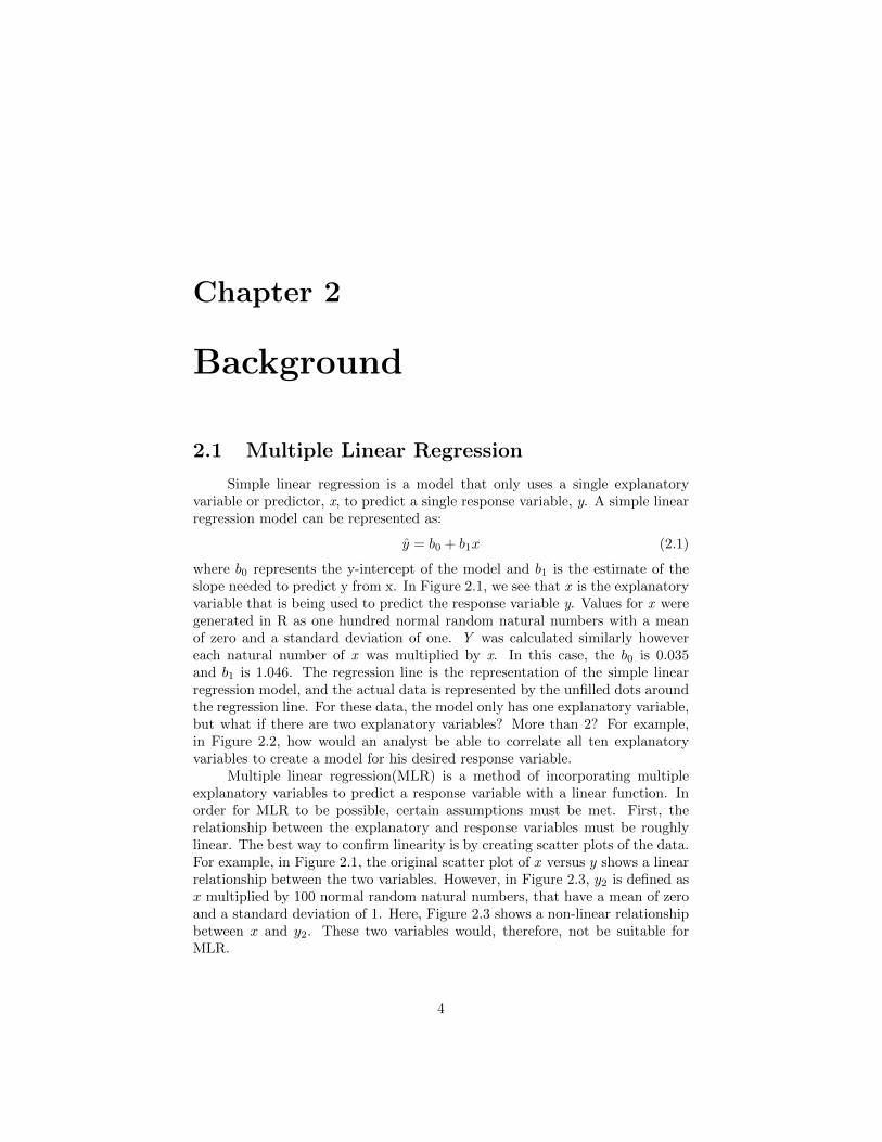
Simple linear regression is a model that only uses a single explanatoryvariable or predictor, x, to predict a single response variable, y. A simple linearregression model can be represented as:

y = b0 + b1x (2.1)

where b0 represents the y-intercept of the model and b1 is the estimate of theslope needed to predict y from x. In Figure 2.1, we see that x is the explanatoryvariable that is being used to predict the response variable y. Values for x weregenerated in R as one hundred normal random natural numbers with a meanof zero and a standard deviation of one. Y was calculated similarly howevereach natural number of x was multiplied by x. In this case, the b0 is 0.035and b1 is 1.046. The regression line is the representation of the simple linearregression model, and the actual data is represented by the unfilled dots aroundthe regression line. For these data, the model only has one explanatory variable,but what if there are two explanatory variables? More than 2? For example,in Figure 2.2, how would an analyst be able to correlate all ten explanatoryvariables to create a model for his desired response variable.

Multiple linear regression(MLR) is a method of incorporating multipleexplanatory variables to predict a response variable with a linear function. Inorder for MLR to be possible, certain assumptions must be met. First, therelationship between the explanatory and response variables must be roughlylinear. The best way to confirm linearity is by creating scatter plots of the data.For example, in Figure 2.1, the original scatter plot of x versus y shows a linearrelationship between the two variables. However, in Figure 2.3, y2 is defined asx multiplied by 100 normal random natural numbers, that have a mean of zeroand a standard deviation of 1. Here, Figure 2.3 shows a non-linear relationshipbetween x and y2. These two variables would, therefore, not be suitable forMLR.

4

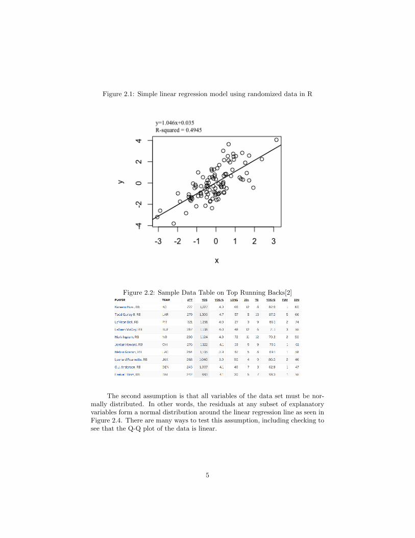
Figure 2.1: Simple linear regression model using randomized data in R

Figure 2.2: Sample Data Table on Top Running Backs[2]

The second assumption is that all variables of the data set must be nor-mally distributed. In other words, the residuals at any subset of explanatoryvariables form a normal distribution around the linear regression line as seen inFigure 2.4. There are many ways to test this assumption, including checking tosee that the Q-Q plot of the data is linear.

5

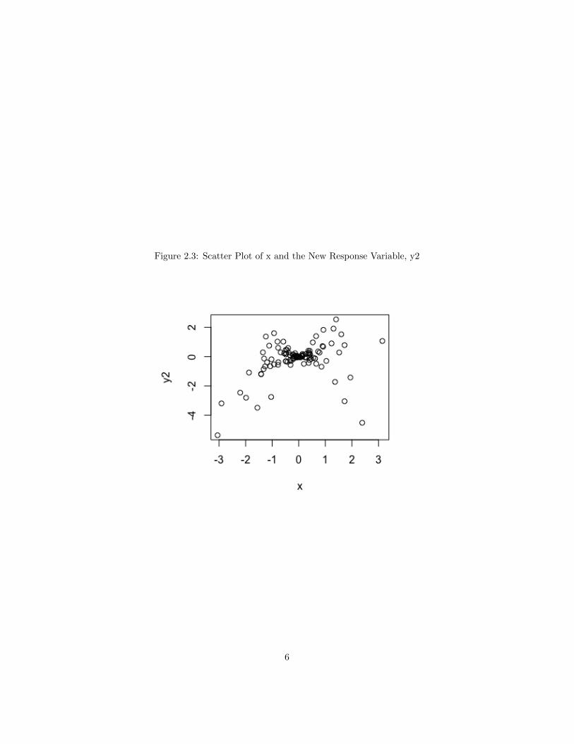
Figure 2.3: Scatter Plot of x and the New Response Variable, y2

6

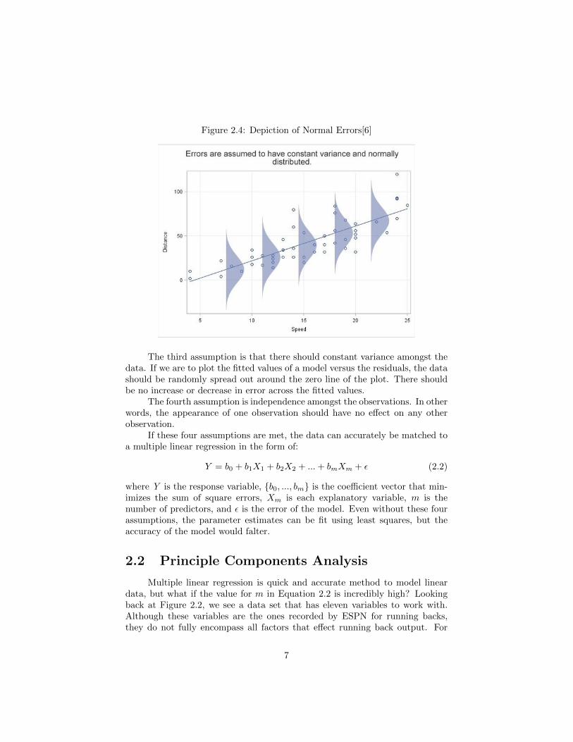
Figure 2.4: Depiction of Normal Errors[6]

The third assumption is that there should constant variance amongst thedata. If we are to plot the fitted values of a model versus the residuals, the datashould be randomly spread out around the zero line of the plot. There shouldbe no increase or decrease in error across the fitted values.

The fourth assumption is independence amongst the observations. In otherwords, the appearance of one observation should have no effect on any otherobservation.

If these four assumptions are met, the data can accurately be matched toa multiple linear regression in the form of:

Y = b0 + b1X1 + b2X2 + ...+ bmXm + ε (2.2)

where Y is the response variable, {b0, ..., bm} is the coefficient vector that min-imizes the sum of square errors, Xm is each explanatory variable, m is thenumber of predictors, and ε is the error of the model. Even without these fourassumptions, the parameter estimates can be fit using least squares, but theaccuracy of the model would falter.

2.2 Principle Components Analysis

Multiple linear regression is quick and accurate method to model lineardata, but what if the value for m in Equation 2.2 is incredibly high? Lookingback at Figure 2.2, we see a data set that has eleven variables to work with.Although these variables are the ones recorded by ESPN for running backs,they do not fully encompass all factors that effect running back output. For

7

example, one variable that is not accounted for in Figure 2.2 is the capability ofone’s offensive line. No matter how talented a running back is, the offensive lineis necessary in creating openings to run through and keeping defenders at bay.Now what are all the factors that contribute to the effectiveness of the offensiveline? We could still use MLR for a large number of explanatory variables, butsome variables like the offensive line, speed of the running back, and others aremore substantial in affecting running back output than variables like a team’swide receiver output. The less important pieces of information can be left outof models as they have little effect on the response variable. However, how canwe decide which variables have more influence on the data?

Principal components analysis (PCA) is a method of analysis that cansolve both of these questions that MLR cannot. When dealing with m numberof of variables, where m is very large, PCA serves to compress the data tobe focused on k components, where k is less than or equal to m. Althoughthe full dataset includes all m variables, the k variables will be able to explainapproximately the same amount of variability in the response variable that them explanatory variables do. Figure 2.5 shows a broad overview of how PCAzooms the scope of the model to only incorporate the most important variables.

In other words, PCA creates linear combinations, or principle components(PC), of all variables to represent the data set. The top image of Figure 2.5depicts a model that uses a set of the original explanatory variables to predicty1. M1 portrays a model that does not have any relation between y1 and x5.M2 utilizes the same five explanatory variables to predict y1. This shows howlinear combinations of x1-x4 can create just two components, C1 and C2. Thesecomponents are then used in a linear model to predict y1. Similarly, PCA canbe used in football data like from Figure 2.2 to compress the enormous numberof variables into fewer variables which are then utilized in a linear model topredict a response variable[4].

8

Figure 2.5: Principle Components Analysis Flow Chart [3]

9

Chapter 3

Mathematical Derivation ofPartial Least Squares

Much like PCA, Partial Least Squares (PLS) aims to compress the orig-inal data matrix in order to create a regression model with fewer explanatorycomponents than number of variables in the original data space. Similarly, PLScreates linear combinations to represent the explanatory variables with latentvariables, and the greater the number of latent variables or components, themore representative of the data these latent variables will be. The sets of lin-ear combinations for both PLS and PCA are from the explanatory variables;however, the key difference between the two modeling techniques lies in theoptimization criteria that created the coefficients. PCA aims to create a lin-ear combination that will project the data onto the one dimensional space thatcaptures the maximum variability in X, but PLS’s goal is to do the same forXTY . We will dive into more depth on how PLS achieves this goal later in thischapter.

Let’s suppose we have a sample of size N which contains the responsevariables Y1,Y2,...,Yp and the explanatory variables X1,X2,...,Xm, where p andm are the number of response and explanatory variables, respectively. Whenp is only one, we have the option of creating a linear regression model of thefollowing form:

Y = XB (3.1)

where the regression coefficients, B, can be estimated with:

B = X+Y (3.2)

Here, X+ is defined as (XTX)−1XT , otherwise known as the matrix pseudoin-verse. However, collinear variables in the X matrix create trouble in this set ofsolutions because XTX must be invertible. The issue of non-invertible XTXmatrices can be solved by using PLS. We must decompose the X and Y matricesinto the following forms:

XN×m = TN×rPTr×m YN×r = TN×rC

Tr×p (3.3)

10

where T is an orthogonal matrix that is common to both X and Y . In PLS,the common matrix T acts to relate the explanatory variables with the responsevariables for more accurate latent variables. The T matrix is arbitrary at themoment, but it is the same matrix in the decomposition of X and Y matrices tomaximize the variability of XTY captured by the linear combination betweenX and Y . P and C are the loadings matrices for X and Y , r is the rankof the input matrix. T , P , and C must be computed iteratively. We mustcalculate a component, w ∈ Rm×1, such that the covariance between X and Yis maximized. Let’s define the matrix, S, as such:

S1 = XT1 Y1 (3.4)

where X1 and Y1 represent the initial conditions of the response and explanatoryvariables. That is, X1 = X and Y1 = Y . The subscripts for these matricesindicate that PLS is a iterative process where each covariance matrix after thefirst is an approximated version of the original data matrices. Because thecovariance equation is cov(X) = XXT if X is centered, we know that thecov(XTY ) = XTY XY T = SST . Based on the initial conditions X1 and Y1, thefirst component vector w1 is the solution to the following optimization problem:

w1 = arg max||w||=1

wTS1ST1 w (3.5)

which then maximizes the cov(w1XTY ). w1 is also the largest eigenvector of

cov(XTY ),w1 = Eigmax{S1S

T1 }. (3.6)

Here, Eigmax{} is the operator that extracts the maximum eigenvector from agiven matrix. We, then, take our newly calculated first component, w1, and useit to calculate the first column of the scores matrix T in the following way:

t1 = X1w1. (3.7)

Eventually, we want to rewrite equation (3.3) as a summation of the multipli-cation between the columns of T and P for X and between the columns of Tand C for Y .

X =

r∑d=1

tdpTd , Y =

r∑d=1

tdcTd (3.8)

However, our PLS equation only calculated the first score, t1, and we do notknow the other column values for the T matrix. This first column of the scoresis used as an approximation of the X and Y matrices as such:

X ≈ t1pT1 , Y ≈ t1cT1 (3.9)

where p1 and c1 are the first columns of their respective loadings matrices.Later, I will show how to calculate X2. P and C have not yet been calculatedso we must figure out a way to determine these values. Upon closer inspection,the equations in (3.9) are similar to equation (3.1). Using least squares as in

11

equation (3.2), we apply the same method to determine the first columns of Pand C. We do so by projecting the values of X1 onto t1 as seen in equation(3.10)

X1 = t1pT1 → p1 = (tT1 t1)−1tT1X1 (3.10)

The Y matrix is treated similarly to calculate c1 as such:

Y1 = t1cT1 → c1 = (tT1 t1)−1tT1 Y1, (3.11)

which simplifies to equation (3.12) determining p1 and c1.

p1 =XT

1 t1tT1 t1

, c1 =Y T1 t1tT1 t1

(3.12)

We then subtract t1pT1 from X to create a new deflated matrix. This process

removes the influence of t1 on the original X and Y matrices, and we are leftwith the following:

X2 ← X1 − t1pT1 , Y2 ← Y1 − t1cT1 (3.13)

In other words, we subtract the component in the direction of the maximumcov(w1X

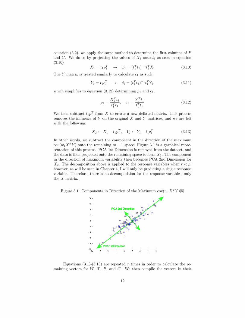
TY ) onto the remaining m − 1 space. Figure 3.1 is a graphical repre-sentation of this process. PCA 1st Dimension is removed from the dataset, andthe data is then projected onto the remaining space to form X2. The componentin the direction of maximum variability then becomes PCA 2nd Dimension forX2. The decomposition above is applied to the response variables when r < p;however, as will be seen in Chapter 4, I will only be predicting a single responsevariable. Therefore, there is no decomposition for the response variables, onlythe X matrix.

Figure 3.1: Components in Direction of the Maximum cov(w1XTY )[5]

Equations (3.1)-(3.13) are repeated r times in order to calculate the re-maining vectors for W , T , P , and C. We then compile the vectors in their

12

respective matrices as such:

W = w1, ..., wr T = t1, ..., tr P = p1, ..., pr C = c1, ..., cr (3.14)

Finally, we are left with a newly formed X matrix marked as:

X = TPT = TPT × I = TPTWWT = T (PTW )WT (3.15)

where I is the identity matrix. The coefficients for this PLS model are calculatedin a similar way as equation (3.2).

B = X+Y (3.16)

X+ is calculated as such:

X+ = (XT X)−1XT (3.17)

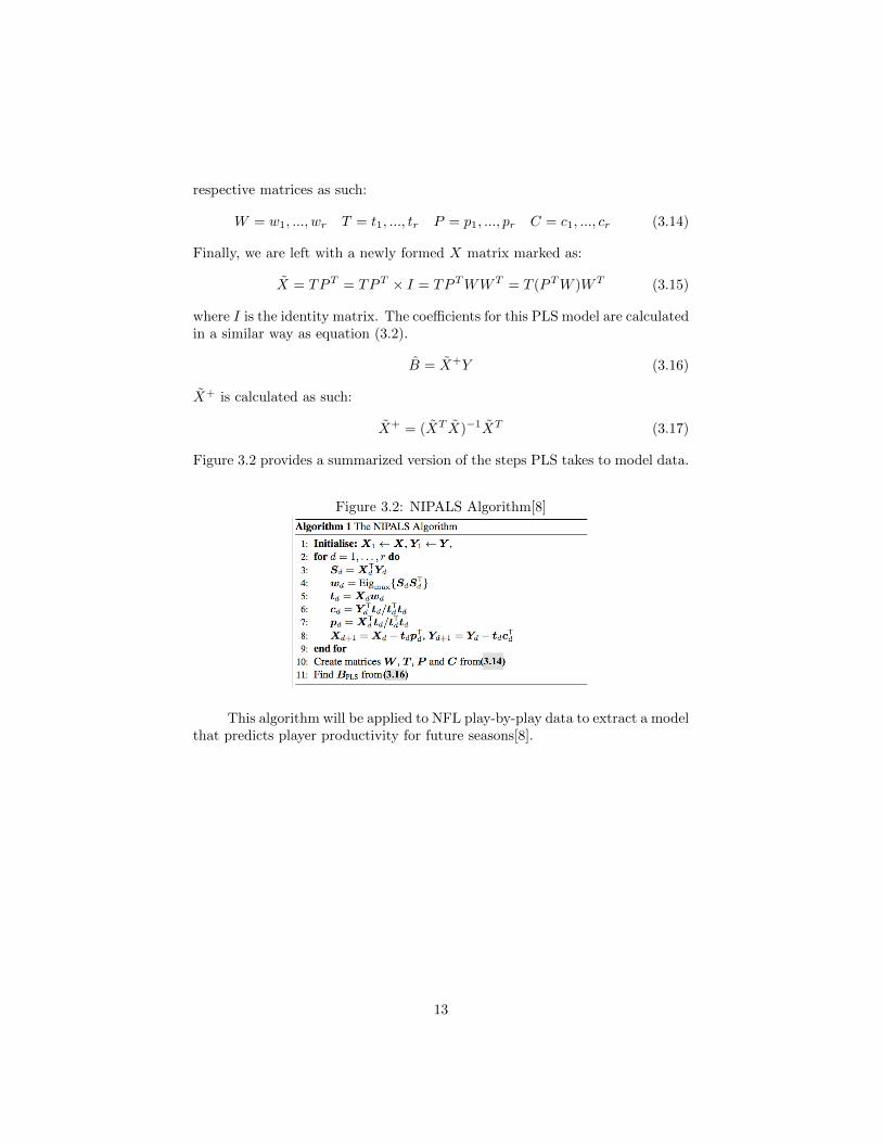
Figure 3.2 provides a summarized version of the steps PLS takes to model data.

Figure 3.2: NIPALS Algorithm[8]

This algorithm will be applied to NFL play-by-play data to extract a modelthat predicts player productivity for future seasons[8].

13

Chapter 4

PLS Application to NFLData

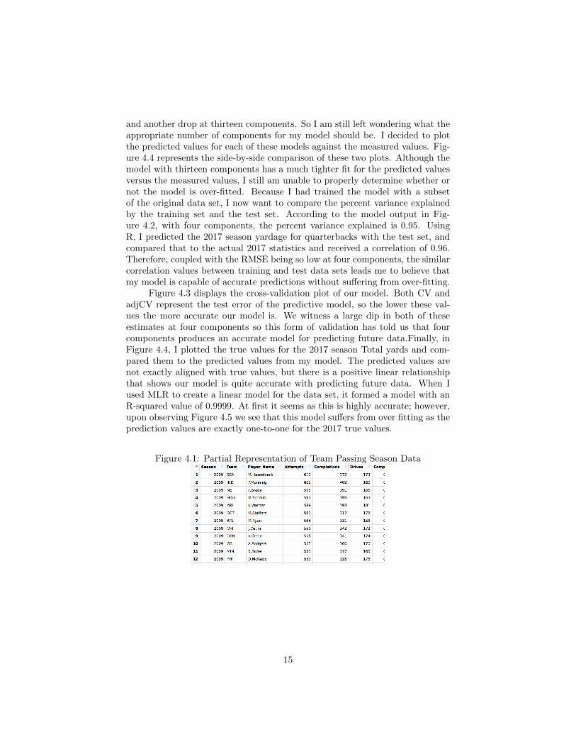
In order to fully grasp the depth of the PLS technique, I have applied itto nine seasons worth of NFL play-by-play data scraped from ryurko’s githubrepository [7]. The play-by-play data displays the time of each play, what typeof play was run, the players involved in the play, the result of the play in termsof yardage or any other event including touchdowns and turnovers, and otherdetails about the play. When approaching these datasets, my focus was to ob-serve a player or team’s output over an entire season rather than just a play at atime. I then began running analysis on the data sets that presented data in sucha fashion seen in Figure 4.1, which presents statistics each team’s quarterbackfrom 2009 to 2017. In Figure 4.1, there seem to only be a few variables, sowouldn’t I just use MLR to model these data? In actuality, this image is onlya small section of the full dataset. The full dataset has 288 observations and88 variables, which makes MLR a less appropriate technique. Thankfully, oneof PLS’s prime objectives is to compress the number of explanatory variables.And so, using R, I applied a PLS Regression model to this dataset that resultedin the output seen in Figure 4.2. The model consisted of just one response vari-able (Total Yardage) and the rest of the dataset as the explanatory variables.I chose twenty components to put into the model in order to as an arbitrarymaximum number of components. From the output in Figure 4.2, I can seethat the percent variance explained in the response variable begins to plateauat four components; however, there seems to be another plateau at thirteencomponents as well. In order to better determine what the appropriate numberof components are to be used in the model. I plotted the root mean squarederror (RMSE) of this model in Figure 4.3. The goal is to minimize the RMSEvalue without running into the dilemma of over-fitting. To detect over-fitting,the model was constructed with a training dataset consisting of data from 2009to 2016. The 2017 season was set aside as the test data set for later use. Justas expected, there is a significant drop until the model reaches four components

14

and another drop at thirteen components. So I am still left wondering what theappropriate number of components for my model should be. I decided to plotthe predicted values for each of these models against the measured values. Fig-ure 4.4 represents the side-by-side comparison of these two plots. Although themodel with thirteen components has a much tighter fit for the predicted valuesversus the measured values, I still am unable to properly determine whether ornot the model is over-fitted. Because I had trained the model with a subsetof the original data set, I now want to compare the percent variance explainedby the training set and the test set. According to the model output in Fig-ure 4.2, with four components, the percent variance explained is 0.95. UsingR, I predicted the 2017 season yardage for quarterbacks with the test set, andcompared that to the actual 2017 statistics and received a correlation of 0.96.Therefore, coupled with the RMSE being so low at four components, the similarcorrelation values between training and test data sets leads me to believe thatmy model is capable of accurate predictions without suffering from over-fitting.

Figure 4.3 displays the cross-validation plot of our model. Both CV andadjCV represent the test error of the predictive model, so the lower these val-ues the more accurate our model is. We witness a large dip in both of theseestimates at four components so this form of validation has told us that fourcomponents produces an accurate model for predicting future data.Finally, inFigure 4.4, I plotted the true values for the 2017 season Total yards and com-pared them to the predicted values from my model. The predicted values arenot exactly aligned with true values, but there is a positive linear relationshipthat shows our model is quite accurate with predicting future data. When Iused MLR to create a linear model for the data set, it formed a model with anR-squared value of 0.9999. At first it seems as this is highly accurate; however,upon observing Figure 4.5 we see that this model suffers from over fitting as theprediction values are exactly one-to-one for the 2017 true values.

Figure 4.1: Partial Representation of Team Passing Season Data

15

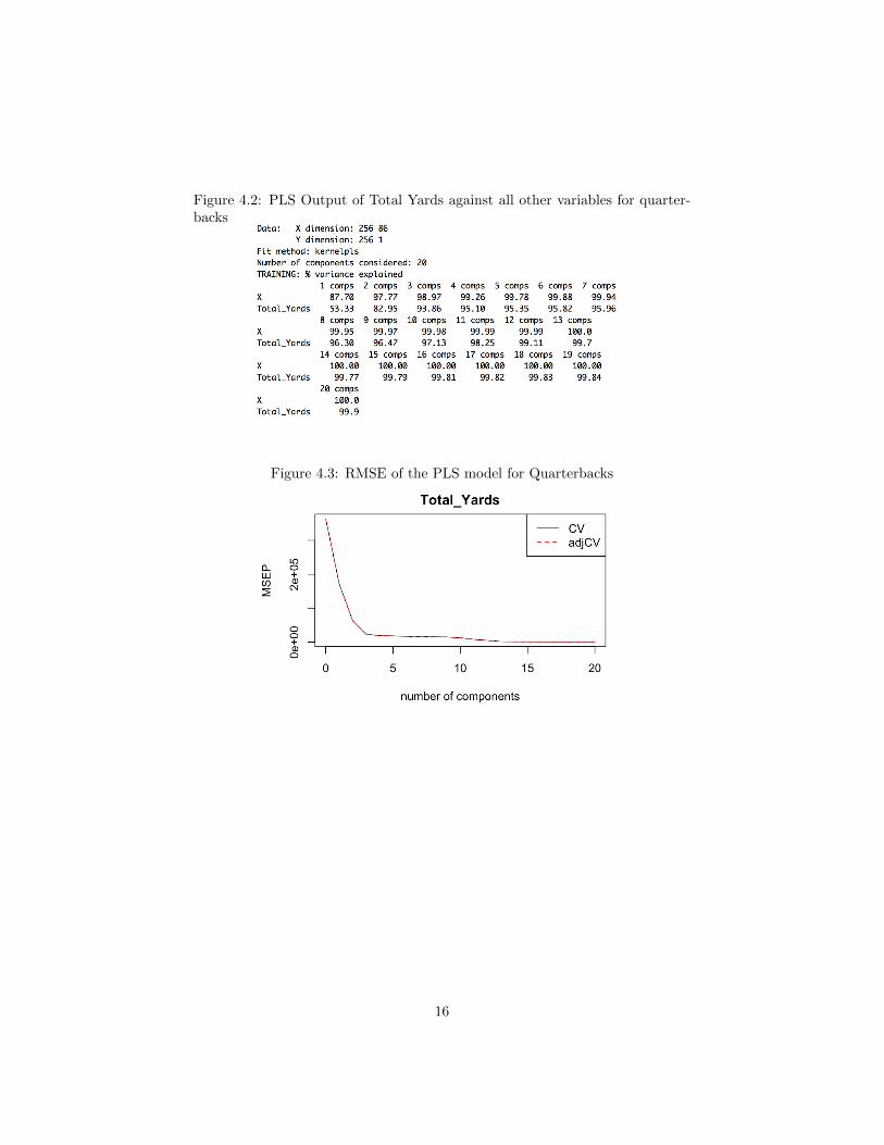
Figure 4.2: PLS Output of Total Yards against all other variables for quarter-backs

Figure 4.3: RMSE of the PLS model for Quarterbacks

16

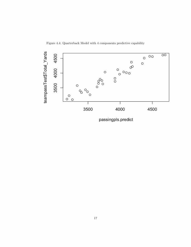
Figure 4.4: Quarterback Model with 4 components predictive capability

17

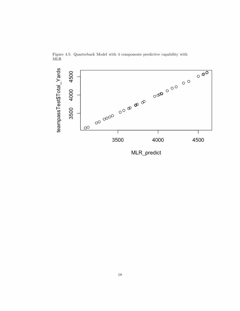
Figure 4.5: Quarterback Model with 4 components predictive capability withMLR

18

Chapter 5

Conclusion

Through the data analysis, I was able to create a model to best repre-sent the quarterback passing data over 8 seasons. The appropriate number ofcomponents for the model was found to be four components in order to avoidover-fitting while still providing a strong enough model for predictive ability.As a general rule of thumb for PLS regression models, the appropriated numberof components for the model can be found by choosing the value with the firstsignificant drop in RMSE value.

In the future, I would like to apply this type of analysis to players in-cluding the running back, wide receivers, tight end, etc. I would also like toresearch the effects that these players have upon each other. In other words,how does a running back’s productivity affect that of the quarterback and viceversa. To do so, I would like to create a numerical rating system for each playerbased off their statistics, and include these values with other player’s stat chartsto observe the correlation between players on the same team. Currently, thereis little data on the effectiveness of the offensive line in these datasets, but Iwould like to be able to incorporate a method of measuring their efficiency andstrength as a variable for the other players as well. One additional metric thatmust be analyzed is each team’s defensive opponents. Clearly, a quarterbackwill perform at a higher level against weaker defenses, but how do we measurea team’s defensive value. Just as there is the quarterback rating(QBR), I wouldlike to create a scale for defenses to be able to account for all factors that influ-ence a player’s productivity. In the long run, these models will be used to createa full team depth chart based off of style of play and effectiveness with each playstyle. The factors that have the most influence on Total Yards or Touchdownscan be isolated using coefficient plots, leading to the areas that need the mostattention while practicing or building a team.

In a perfect world (with more time), I would also create models with MLRand PCA. I could then compare the accuracy and analyze the difference betweenall three modeling techniques. They each have their own advantages and disad-vantages with respect to predictive capability, so it is important to understandwhich data sets require each technique.

19

Bibliography

[1] Chris Ciovacco. Bullish or bearish stocks? www.seeitmarket.com/

bullish-or-bearish-stocks-what-the-charts-are-saying-14335/.

[2] ESPN. Rushing yards leaders. www.espn.com/nfl/statistics/player/-/stat/rushing/sort/rushingYards/seasontype/2.

[3] Stack Exchange. Do the problems of stepwise variable selection exist infa, pca, sem? https://stats.stackexchange.com/questions/231412/

do-the-problems-of-stepwise-variable-selection-exist-in-fa-pca-sem.

[4] Richard Johnson and Dean Wichern. Applied Multivariate Statistical Anal-ysis. Prentice Hall, Inc., 1992.

[5] Guoxin Li. How do i interpret the results of a pca analysis? https://www.

quora.com/How-do-I-interpret-the-results-of-a-PCA-analysis.

[6] Quora. What are the difference errors and residuals in regression analysis,for example, linear regression?

[7] ryurko. nflscrapr-data. https://github.com/ryurko/nflscrapR-data.

[8] Alexander E. Stott, Sithan Kanna, Danilo P. Mandic, and William T. Pike.An online nipals algorithm for partial least squares.

20