Embed Size (px)
Citation preview

Institutionen för Matematik och Fysik Code: MdH-IMa-2005:015
MASTER THESIS IN MATHEMATICS /APPLIED MATHEMATICS
A Java Applet for pricing Bonds and Bond Options using the
Black-Derman-Toy model
by
Zhang Lei
Magisterarbete i matematik / tillämpad matematik
DEPARTMENT OF MATHEMATICS AND PHYSICS MÄLARDALEN UNIVERSITY
SE-721 23 VÄSTERÅS, SWEDEN

DEPARTEMENT OF MATHEMATICS AND PHYSICS ___________________________________________________________________________ Master thesis in mathematics / applied mathematics Date: 2005-10-26 Projectname: A Java Applet for Pricing Bonds and Bond Options using the Black-Derman-Toy model Author: Zhang Lei Supervisor: Jan Röman Examiner: Anatoliy Malyarenko Comprising: 10 points ___________________________________________________________________________

Abstract There are seven parts in this thesis report. Part one: Introduction gives information about background, purpose of study and using methods. Part two: The Black-Derman-Toy model gives the detail of the definition, using one example to show how the theory could be used for backward induction and also another graphical example to show how to build up the binomial lattice model. Part three: Brownian-Path Independent Interest models explain the green function and forward induction method. BDT model could be used only to fit to the yield curve, and also could fit to both interest rate yield and volatility data. Part four: Bond and option pricing describes how to calculate the discount factor tree, Zero-coupon bond, calculate market price from a given spread and calculate spread from a given market price. In the option pricing part, we gives graphical examples by using European call and put, American call and put and Bermudan call and put options to show how BDT model be used for pricing bond options. Part five: User’s Guide. This is the main part of the whole work. We use earlier knowledge of Analytical Finance II together with Java in Analytical Finance, in order to create a Java Applet that Pricing Bonds and bond Options using The Black-Derman-Toy Model and shows results graphically. Part six: Conclusion focuses on the purpose of this study. In the end, three important appendixes, such as fitting yield curves with maximum smoothness, the Newton-Raphson method in 2 dimensions and the Java Applet code has been presented.

- 1 -
Acknowledgements The writing of this thesis gives me an invaluable knowledge how to make a project alive from the state of idea generation to a concrete paper, and to explore the basic knowledge of earlier experience. From my very personal point of view, I think the major point with this study is to understand financial results by using mathematical models. Along with the theories, an applet is built for Java. I sincerely thank Jan Röman for his help and advice during the life of the project.

- 2 -
Table of contents 1 Introduction.............................................................................................................- 3 -
1.1 Background.....................................................................................................- 3 - 1.2 Purpose of Study .............................................................................................- 3 - 1.3 Method ............................................................................................................- 3 -
2 The Black Derman Toy model................................................................................- 4 - 2.1 Definition: .......................................................................................................- 4 - 2.2 Example of using backward induction............................................................- 5 - 2.3 Binomial Lattice model.................................................................................- 12 -
3 Brownian-Path Independent Interest Models........................................................- 15 - 3.1 The Green function and the forward induction method................................- 16 - 3.2 BDT model fitted to the yield curve only .....................................................- 17 - 3.3 BDT model fitted to interest rate yield and volatility data ...........................- 19 -
4 Bond and option pricing........................................................................................- 22 - 4.1 Calculating the discount factor tree ..............................................................- 22 - 4.2 Zero-Coupon bond........................................................................................- 23 - 4.3 Coupon paying bond.....................................................................................- 24 - 4.4 Spread and market price................................................................................- 25 -
4.4.1 Calculate market price from a given spread .........................................- 26 - 4.4.2 Calculate spread from a given market price .........................................- 27 -
4.5 Option pricing ...............................................................................................- 28 - 4.5.1 European call option .............................................................................- 29 - 4.5.2 European put option..............................................................................- 29 - 4.5.3 American call option.............................................................................- 30 - 4.5.4 American put option .............................................................................- 31 - 4.5.5 Bermudan call option............................................................................- 32 - 4.5.6 Bermudan put option.............................................................................- 33 -
5 User’s Guide .........................................................................................................- 35 - 6 Conclusion ............................................................................................................- 41 - 7 Appendixes ...........................................................................................................- 42 -
7.1 Fitting yield curves with maximum smoothness ..........................................- 42 - 7.2 The Newton-Raphson method in 2 dimensions ............................................- 45 - 7.3 Java Applet code ...........................................................................................- 48 -
References.....................................................................................................................- 67 -

- 3 -
1 Introduction
1.1 Background In 1991 Black and Karasinski generalized the Black-Derman-Toy model. This one-factor model is one of the most used yield-based models to price bonds and interest-rate options. The model is arbitrage-free and thus consistent with the observed term structure of interest rates. The family of a financial option is a general term denoting the class into which the option falls, usually defined by the dates on which the option may be exercised. The vast majority of option contracts are either European or American style options. Under normal American option, there exists a type of non-standard American option, called Bermudan option. Java is a programming language developed by Sun Microsystems. The syntax of Java is much like that of C/C++, but it is object-oriented and structured around "classes" instead of functions. Java can also be used for programming applets -- small programs that can be embedded in Web sites. The language is becoming increasingly popular among both Web and software developers since it is efficient and easy-to-use.
1.2 Purpose of Study The purpose of this thesis is to use the Black-Derman-Toy model to value cash flow instruments, such as: bonds, bond options and callable/put able bonds with OAS. The input of data and results will be given in a web-based Graphical User Interface (GUI). The preferred code will be written as a Java applet to be presented at the Internet.
1.3 Method The descriptions and analysis of theories are based mainly on student literature from courses Analytical Finance I and Analytical Finance II. Also, there is reliable secondary information gathered from Internet that has been used. The Java Applet program used to build the graphical User Interface (GUI) part is based on course Java in Analytical Finance. Extra study material literature was supplied by the project supervisor.

- 4 -
2 The Black Derman Toy model
2.1 Definition:1 The Black-Derman Toy model is a one factor short-rate model and is one of the most used yield-based models to price bonds and interest-rate options. It was generalized by Black and Karasinski and first presented in an article published in the Financial Analyst Journal in 1990. The model is arbitrage-free and it is developed to match the observed term structure of yields on zero coupon bonds and their corresponding volatilities. Short rates are lognormally distributed at all times. Short-rate volatility is potentially time dependent, and the continuous process of the short-term interest rate is given by:
( ) ( ) ( )( ) ( ) ( )dztdttrttttrd σ
σσθ +
+= lnln
'
( 2.1)
Where σ´(t)/σ(t) is the speed of mean reversion (“gravity”), and θ(t) divided by the speed of mean reversion is a time-dependent mean-reversion level. The BDT model incorporates as we see, two independent functions of time, θ(t) and σ(t), chosen so that the model fits the term structure of spot interest rates and the term structure of spot rate volatilities. The changes in the short rate are lognormally distributed, with the resulting advantage that interest rates cannot become negative. Once θ(t) and σ(t) are chosen, the future short-rate volatility, by definition, is entirely determined. The model has the advantage that the volatility unit is a percentage, conforming to the market convention. Unfortunately, due to its lognormality, neither analytic solutions for the prices of bonds or the prices of bond options are available, nor numerical procedures are required to derive the short-rate tree that correctly returns the market term structures. Many practitioners choose to fit the rate structure only, holding the future short-rate volatility constant. The convergent limit therefore reduces to the following:
( ) ( )dztdttdInr σθ += ( 2.2 )
This version can be seen as a lognormal version of Ho-Lee model.
1 Haug, E., The Complete Guide to option Pricing Formulas. McGraw-Hill
- 5 -
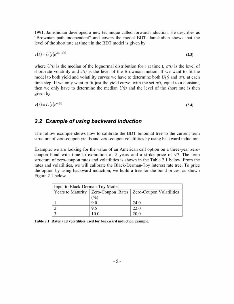
1991, Jamshidian developed a new technique called forward induction. He describes as “Brownian path independent” and covers the model BDT. Jamshidian shows that the level of the short rate at time t in the BDT model is given by ( ) ( ) ( )tztetUtr )(σ= (2.3)
where U(t) is the median of the lognormal distribution for r at time t, σ(t) is the level of short-rate volatility and z(t) is the level of the Brownian motion. If we want to fit the model to both yield and volatility curves we have to determine both U(t) and σ(t) at each time step. If we only want to fit just the yield curve, with the set σ(t) equal to a constant, then we only have to determine the median U(t) and the level of the short rate is then given by ( ) ( ) ( )tzetUtr σ= (2.4)
2.2 Example of using backward induction The follow example shows how to calibrate the BDT binomial tree to the current term structure of zero-coupon yields and zero-coupon volatilities by using backward induction. Example: we are looking for the value of an American call option on a three-year zero-coupon bond with time to expiration of 2 years and a strike price of 90. The term structure of zero-coupon rates and volatilities is shown in the Table 2.1 below. From the rates and volatilities, we will calibrate the Black-Derman-Toy interest rate tree. To price the option by using backward induction, we build a tree for the bond prices, as shown Figure 2.1 below.
Input to Black-Derman-Toy Model Years to Maturity Zero-Coupon Rates
(%) Zero-Coupon Volatilities
1 9.0 24.0 2 9.5 22.0 3 10.0 20.0
Table 2.1. Rates and volatilities used for backward induction example.

- 6 -
Figure 2.1. Bond price tree.
In order to build the price tree, we need to build the rate tree below, Figure 2.2:
Figure 2.2. Rate tree.
Now we will find the prices of the zero-coupon bonds with maturity from one year to three year in the future. By using the zero-coupon rate are shown in the table above and the face value are 100 (% of the nominal amount). We got:
74.9109.01
100=
+
( )40.83
095.01100
2 =+
( )13.75
10.01100
3 =+
r ru
rd
ruu
rud
rdd
S Su
Sd
Suu
Sdd
Sud
100
100
100
100

- 7 -
Then we add this to our data below, Table 2.2
Years to Maturity
Zero-Coupon Rates (%)
Zero-Coupon Volatilities
Zero-Bond Prices
1 9.0 24.0 91.74 2 9.5 22.0 83.40 3 10.0 20.0 75.13
Table 2.2. Calculated input refer to table 2.1.
Then give us a one-period price tree:
Figure 2.3. One period price tree.
The next step is to build a two-period price tree. As shown in the table 2.2 above, it is clear that the price today of a two-year zero-coupon bond with maturity two years from today must be 83.40. To find the second-year bond prices at year one, we need to know the short rates at step one:
Figure 2.4. Two period price tree and one period rate tree.
Appealing to risk-neutral valuation, the following relationship must hold:
40.8309.01
11005.0
11005.0
=+
+⋅+
+⋅
ud rr ( 2.5)
In a standard binomial tree, we have
83.40 Su
Sd
100
100
100
ru
rd 9.0
91.74 100
100

- 8 -
teu ∆= σ ( 2.6)
ted ∆−= σ ( 2.7)
tduIne
du t ∆=
⇒= ∆ σσ 22 ( 2.8)
∆=
duIn
t21σ ( 2.9)
+=
+=
dd
uu
rS
rS
1100
1100
( 2.10)
Where ∆t in the situation above is one year. Similarly, in the BDT tree, the rates are assumed to be log-normally distributed. This implies that
22.05.02
1=
⋅=
∆=
d
u
d
un r
rIn
rr
Int
σ
We define the volatility factor Zn by:
tn
neZ ∆= σ2 ( 2.11)
Now left two equations with two unknowns, there are ru and rd. Since ru = rdZn = rde0.44, this leads to the following quadratic equation:
40.8309.01
11005.0
11005.0 44.0
=+
⋅+⋅+
+⋅
err dd ( 2.12)
By solving this equation and discarding the negative solution (a rate can not be negative), we get the following rates at step one:
%87.7=dr , %22.12=ur

- 9 -
Using these solutions, it is now possible to calculate the bond prices that correspond to these rates. The two-step tree of prices then becomes shown Figure 2.5 :
Figure 2.5. Two period price tree.
The next step is to fill in the two-period rate tree.
Figure 2.6. Two period rate tree.
Last time, there were two unknown rates, and two sources of information:
• Zero-coupon rates. • The volatility of the zero-coupon rates.
This time, we have three unknown rates, but still only two sources of information. To get around this problem, remember that the BDT model is built on the following assumptions:
• Rates are lognormally distributed. • The volatility is only dependent on time, not on the level of the short rates. There
is thus only level of volatility at the same time step in the rate tree. Therefore, the step between the rates is given by:
40.020.0223
3 eeeZ t === ⋅∆σ
9.0% 12.22%
7.87%
ruu
rud
rdd
83.40 89.11
92.70
100
100
100

- 10 -
3Zrr
rr
dd
ud
ud
uu == ( 2.13)
Now we left only two unknowns. Based on the risk-neutral valuation principle, the following relationships must hold:
231
1001100
ZrrS
uuuuuu ⋅+
=+
= ( 2.14)
31100
1100
ZrrS
ddudud ⋅+
=+
= ( 2.15)
dddd r
S+
=1100
( 2.16)
1222.015.05.0
+⋅+⋅
= uduuu
SSS ( 2.17)
0787.015.05.0
+⋅+⋅
= ddudd
SSS ( 2.18)
09.015.05.0
13.75+
⋅+⋅= du SS
If the bond only has two years left to maturity, the bond yield or rate of return must Satisfy:
09.010787.01
11005.0
11005.0
5.01222.01
11005.0
11005.0
5.013.75
3323
++
+⋅+
⋅+⋅
⋅++
⋅+⋅+
⋅+⋅
⋅=
dddddddd rZrZrZr
By solving this equation and again discarding any negative answer, we get rdd, then by multiplying with Z3 we get rud and ruu:
%47.7=ddr , %76.10=udr , %50.15=uur

- 11 -
This gives the following rate tree:
Figure 2.7. Two period rate tree.
With these values for r the equations (2.14 – 2.18) above for the S tree can be solved:
58.861100
=+
=uu
uu rS
29.90
1100
=+
=ud
ud rS
05.93
1100
=+
=dd
dd rS
80.781222.01
5.05.0=
+⋅+⋅
= uduuu
SSS
98.840787.01
5.05.0=
+⋅+⋅
= ddudd
SSS
This gives the following three-year price tree:
Figure 2.8. Three period price tree.
9% 12.22%
7.87%
15.50%
10.76%
7.47%
75.13 78.8
84.98
86.58
93.05
90.29
100
100
100
100

- 12 -
The value of the American call option from above is found by standard backward induction:
+−+⋅+++⋅
−=),(1
)1,1(5.0)1,1(5.0,90),(max),(jmr
jmCjmCjmSjmC ( 2.19)
Figure 2.9. American call option value tree.
The calculated price is therefore 0.77.
2.3 Binomial Lattice model Now we will describe the implementation of the model using a binomial lattice. The unit time is divided into M period of length ∆t = 1/M each. At each period m, corresponding to time t = n/M = n∆t, there are n+1 states, which the range from j = -m, -m+2,…, m-2, m. At the present period m = 0, there is a single state j = 0. As shown in the Figure 2.10.
Figure 2.10. Four period binomial lattice.
0 -1
1
-2
0
2
-1
-3
1
3
-2
-4
0
2
4
0.77 0.132
1.55
0
0.296
3.05

- 13 -
Let rm,j denote the annualized one-period rate at period m and state j. Denote the discount factor at period m and state j by:
( )( )[ ] tjmr
jmp ∆+=
,11, (2.20)
Below is one example with the five-step tree of discount factors in Figure 2.11.
Figure 2.11. Five-steps discount factor tree.
As shown in the figure 2.11 is a discrete time representation of the stochastic process for the short rate. We can use equation 2.20 to explain the discount factors instead of the one period rate at each node. The probability for an up or down move in the tree is chosen to be ½. Now we say that the advantage of the binomial lattice model that is once the one period discount factors p(m,j) are determined, thus made securities are evaluated easily by backward induction. So now we let C(m,j) denote the price of a security at period m and state j. This price will get from its prices at the up and down nodes in the next period by the backward equation.
( ))1,1()1,1(),(21),( −++++= jmCjmCjmpjmC ( 2.21)
P1,-1
p1,1
p2,-2
p2,0
p2,2
p3,-1
p3,-3
p3,1
p3,3
p4,-2
p4,-4
p4,0
p4,2
p4,4
p0,0

- 14 -
Figure 2.12. One period price tree.
If we continue all the way backwards to period m = 0 in equation 2.21.We get the price today, C(0,0).
C(m,j) C(m+1,j+1)
C(m+1,j-1)

- 15 -
3 Brownian-Path Independent Interest Models2 This section will talk about the Brownian-Path Independent interest models, and the BDT model which is included in these. By definition, an interest rate model is referred to as Brownian Path Independent (BPI) if there is a function r(z(t), t) such that r(t) = r(z(t), t), where z(t) is the Brownian motion. At any time t the instantaneous interest rate and therefore the entire yield curve depends on z(t) but not on the prior history z(s), s < t of the Brownian motion. Two types of BPI are most interesting:
Normal BPI )()()()( tzttUtr NN σ+= (3.1)
Lognormal BPI )()()()( tztL
LetUtr σ= (3.2)
Where σN(t) and σL(t) represent, respectively the absolute and the percentage volatility of the short rate r(t). UN(t) is the mean and UL(t) the median of r(t). The advantages with the lognormal BPI are as we have mentioned the positive interest rates and natural unit of volatility in percentage form, consistent with the way volatility is quoted in the market place. However, unlike the normal BPI, the lognormal BPI does not provide a closed form solution. It is possible to fit the yield curve by trial and error but this is inefficient. In fact, the total computational time needed to calculate the entire discount factors of a tree with N periods is proportional to N3. If N is a high number, say at least 100, too many iterations are needed. Forward induction efficiently solves the yield curve fitting problems, but before describing the procedure a discrete version of the BPI models is necessary. Consider again the figure 2.10 previously. Define the variable Xk as
∑=
=k
jjk yX
1 Where yj = 1 if an up move occurs at period k and yj = -1 if a down move occurs at period k. The variable Xk gives the state of the short rate at period k. At any period k, the Xk has a binomial distribution with mean zero and variance k. Now, let us investigate the mean and variance of Xk∆t0.5. { } { } 0=∆=∆ kk XEttXE (3.3)
2 Jan Röman, Lecture Notes in Analytical finance II, pp190. 2005

- 16 -
{ } { } 0=∆=∆=∆ tkXtVartXVar kk (3.4)
It follows that Xk∆t0.5 has the same mean and variance as the Brownian motion z(t). Since the normal distribution is a limit of binomial distributions, and the binomial process Xk has independent increments, the binomial process Xk∆t0.5 converges to the Brownian motion z(t) as ∆t approaches zero. The state of the short rate was denoted by j. Replacing Xk by j will lead to having z(t) approximated as j∆t0.5. Now, replacing t by m (with m = t/∆t ) gives the discrete version of the normal and lognormal BPI families.
Normal BPI: ( ) timmUr NNjm ∆+= )(, σ (3.5)
Lognormal BPI: ( ) timLjm
LemUr ∆= )(,
σ (3.6)
This lognormal BPI formula 3.6 is to build a tree for the short rate in the applet.
3.1 The Green function and the forward induction method3 Green function is known as Arrow-Debreu prices in discrete-time finance. Arrow-Debreu prices represent prices of primitive securities. By definition, let G(n,i,m,j) denote the price at period n and state i of a security that has a cash flow of unity at period m ≥ n and state j. Note that G(m,j,m,j) = 1 and that G(m,i,m,j) = 0 for i ≠ j. In most cases we ignore the first two denotations and say that G(m,j) = 1 if we reach the node (m,j) and zero else. We can compute G(m,j) with the forward induction:
( )
( ) ( ) ( ) ( )[ ]
( ) ( )
( ) ( )
++
−−
−−+++
=+
1,1,21
1,1,21
1,1,1,1,21
,1
jmGjmp
jmGjmp
jmGjmpjmGjmp
jmG
1,
1,
1,
−−=
+=
−≤
mj
mj
mj
(3.7)
Where p(m,j) is the one-period discount factor:
( )( )[ ] tjmr
jmp ∆+=
,11, (3.8)
3 Jan Röman, Lecture Notes in Analytical finance II, pp193. 2005

- 17 -
The initial condition is given by G(0,0) = 1. Note that an arbitrary short-rate security expiring at t = m, with a payoff P(m) can be considered as a combination of pure-state securities. The equation (3.7) is the binomial forward induction. We can see that the forward induction function states how we discount a cash flow of unity for receiving it one period later. This is also can be expressed by use the binomial lattice model. Remember if j = ±m, there is only one node (at the bottom or at the top), which gives a modified expression for these two cases. The term structure P(0,m) which represent the price today of a bond that pays unity at period m, can be obtained for all values of m, by the maximum smoothness criterion (see appendix 7.1) Arrow-Debreu prices are the building blocks of all securities. The price of a zero-coupon bond which matures at period m + 1 can be expressed in terms of the Arrow-Debreu prices and the discount factors in period m. ( ) ( ) ( )∑=+
jjmGjmpmP ,,0,0,1,0 (3.9)
In most cases we simply write this equation as ( ) ( ) ( )∑=+
j
jmGjmpmP ,,1 (3.10)
The term structure can be fitted to any Brownian path independent models using forward induction. First, assume that σ(m) = σ is a given constant. We need to solve U(m) to match the given discount function p(m,j) where:
( )( )[ ] ttjemU
jmp ∆∆+=
σ1
1, (3.11)
3.2 BDT model fitted to the yield curve only As we mentioned before that many practitioners when using the BDT model, they set the short-rate volatility to be a constant, and it only will fit to the yield curve. Now we let σ(m) = σ. Let m > 0 and assume that U(m - 1), G(m – 1,j), r(m – 1,j) and p(m – 1,j) have been found. The values at the initial time m = 0 are U(0) = r(0,0), G(0,0) = 1 and p(0,0) = 1/[1+r(0,0)]∆t.

- 18 -
Step 1: Generate the Green functions:
( )
( ) ( ) ( ) ( )[ ]
( ) ( )
( ) ( )
++
−−
−−+++
=+
1,1,21
1,1,21
1,1,1,1,21
,1
jmGjmp
jmGjmp
jmGjmpjmGjmp
jmG
1,
1,
1,
−−=
+=
−≤
mj
mj
mj
Step 2: Use P(m+1) to solve U(m) by use :
( ) ( )( )[ ] ttjj emU
jmGmP ∆∆+=+ ∑
σ1
1,1 ( 3.12)
Step 3: From U(m) calculate the short rate, and update the discount factors, for all nodes at time m: ( ) ( ) tjemUjmr ∆= σ,
( )( )[ ] tjmr
jmp ∆+=
,11,
For the solution in step 2, we use a Newton-Raphson method:
( )( )n
m
nmn
mnm xf
xfxx
'1 −=+ ( 3.13)
We can easily do this since we have the derivatives. Let U(m) = xm be the unknown, then
( ) ( ) [ ] ( )∑ =+−+
= ∆∆jttj
m
m mPex
jmGxf 011
1,σ
( 3.14)

- 19 -
The derivatives are given by
( ) ( ) [ ]∑ +∆∆
∆
+
∆=
jttj
m
tj
mex
tejmGxf 11
,'σ
σ
( 3.15)
3.3 BDT model fitted to interest rate yield and volatility data Now we will fit to both the yield and volatility curves in BDT model. This requires solving U(m) and σ(m). Let PU(m) and PD(m) represent the prices at period n = 1 states of m-maturity zero-coupon bonds. Note that according to the definition of the volatility an up move of the short rate differs from a down move by a factor e2σ(m)∆t^0.5. Therefore we have:
( )( )
( ) tm
D
U termemymy ∆= σ2 ( 3.16)
Where y±(m) denote the yield corresponding to PU(m) and PD(m). Solving for σterm(m)∆t0.5 in equation (3.16) yields,
( ) ( ) ( )
( ) ( ) 1
11
1
11
2
−
−=
∆−−
∆−−∆
tmD
tmUtm
mP
mPe termσ , 2≥m ( 3.17)
A second equation for PU(m) and PD(m) is found by discounting back to the origin.
( ) ( ) ( )[ ] ( )jmpmPmPmP DU ,21
+= , 2≥m ( 3.18)
These two equations can be combined and PU(m) isolation to:
( ) ( )( ) ( ) ( )( )jmp
mPePemPtm
ttmU
tU ,
211
2112 =⋅+−+
∆−−∆−∆−
−∆− σσ ( 3.19)
This equation is solved using Newton Raphson, PD(m) is then:

- 20 -
( ) ( )( ) ( ) tmttm
Ut
D ePemP∆−−
∆−∆−−∆− ⋅+−=
121
121 σσ ( 3.20)
Forward induction is again used to determine the time-dependent functions that ensure consistency with the initial yield curve data. However, state prices are now determined from the nodes U and D requiring the following notation: GU(m,j): the value, as seen from node U, of a security that pays off $1 if node (m, j) is reached and zero otherwise. GD(m,j): the value, as seen from node D, of a security that pays off $1 if node (m, j) is reached and zero otherwise. By definition GU(1,1) = 1 and GD(1,-1) = 1. The tree is constructed from time ∆t onward using a procedure similar to the last section. Now we have two equations:
( ) ( ) ( )( ) ( ) ( )
=+=+
∑∑
jmpjmGmPjmpjmGmP
DD
UU
,,1,,1
( 3.21)
where j = -m, -m + 2,…, m - 2, m and
( )( ) ( )[ ] ttjmemU
jmp ∆∆+=
σ1
1,
The term structure of zero-coupon bonds P(m) and the yield volatility term structure σterm(m) are known. U(m) and σ(m) are two unknown sets, we can solve them by use a two-dimensional Newton-Raphson technique. (See appendix 7.2) The full set of steps to build the tree is therefore the following. Assume m > 0 and that U(m-1), σ(m-1), GU(m-1,j), GD(m-1,j) and r(m-1,j) are known for all j at time step m – 1. The values at initial time are U(0,0) = r(0,0), σ(0) = σterm(1), GU(1,1) = 1, GD(1,-1) = 1 and r(m-1,j) giving p(0,0) = 1/[1+r(0,0)]∆t. Step 1: Derive PU(m) and PD(m) for m = 2 to N.
( ) ( )( ) ( ) tmttm
Ut
D ePemP∆−−
∆−∆−−∆− ⋅+−=
121
121 σσ PU(m) is found as the solution to

- 21 -
( ) ( )( ) ( ) ( )( )jmp
mPePemPtm
ttmU
tU ,
211
2112 =⋅+−+
∆−−∆−∆−
−∆− σσ
Step 2: Generate GU(m,j), GD(m,j):
( ) ( ) ( ) ( ) ( )[ ]
( ) ( ) ( ) ( ) ( )[ ]
+−+−+−−−−=
+−+−+−−−−=
1,11,11,11,121,
1,11,11,11,121,
jmGjmpjmGjmpjmG
jmGjmpjmGjmpjmG
DDD
UUU ( 3.22)
Step 3: Using the derived discount functions PU(m+1) and PD(m+1), solve U(m) and σ(m) from
( ) ( ) ( )( ) ( ) ( )
=+=+
∑∑
jmpjmGmPjmpjmGmP
DD
UU
,,1,,1
Where j = -m, -m + 2,…, m - 2, m and
( )( ) ( )[ ] ttjmemU
jmp ∆∆+=
σ1
1,
Step 4: From the calculated values of U(m) and σ(m) calculate the short rate, and one period discount factors for all nodes j at time m: ( ) ( ) ( ) tjmemUjmr ∆= σ,
( )[ ( ) ] tjmr
jmp∆+
=,1
1,
The method of forward induction requires only n arithmetic operations to construct the discount factors at period n. The iterations are made only on the nodes at the given period, not the whole way back to the root of the tree as in "trial and error". In a tree with N periods, the computational time is proportional to the number of nodes N2, which is of the same order as when closed formed solutions for the discount factors are available.

- 22 -
4 Bond and option pricing This chapter will discuss and describe how to price bonds and options on those bonds using the BDT forward induction model. All calculations are done by the Java applet produced together with this thesis which uses the theory from chapter 2 and 3.
4.1 Calculating the discount factor tree The first thing needed in pricing bonds and options is the rate and discount factor trees. Table 4.1 below gives the assumed market term structure. Maturity: m(years)
Zero-Coupon Bond: P(0,m) (paying $1 in m years)
Yields: y (m) (%)
Yield Volatility: σterm(m) (%)
1 0.9524 5 21 2 0.8900 6 20 3 0.8163 7 19 4 0.7350 8 18 5 0.6499 9 17
Table 4.1. Rates and volatilities used for bond and option examples.
These values are inserted in the Java applet which calculates the rate tree shown in Figure 4.1 and the discount factor tree as shown in Figure 4.2.
0.0699 0.0653 0.0611 0.0947 0.0564 0.0912 0.05 0.088 0.1282 0.0841 0.1273 0.1269 0.1737 0.1777 0.2352
Figure 4.1. Rate tree.

- 23 -
0.9347 0.9387 0.9424 0.9135 0.9466 0.9164 0.9524 0.9191 0.8863 0.9224 0.8871 0.8874 0.852 0.8491 0.8096
Figure 4.2. Discount factor tree.
4.2 Zero-Coupon bond Once the discount factor tree has been calculated it can be used to calculate the bond price tree for zero-coupon bond. The price at maturity is known to be unity (100%). The discount factors from Figure 4.2 are then used to calculate the bond prices before that date using the equation for the bond price tree below.
( ) ( ) ( ) ( )[ ]1,11,1,21, −++++⋅= jmPjmPjmpjmP ( 4.1)
P(m+1,j+1)P(m,j) P(m+1,j-1)

- 24 -
This gives the zero-coupon bond price tree as follows:
100.0 93.4651 86.7437 100.0 79.739 91.3504 72.4501 82.4736 100.0 64.9931 73.3342 88.6347 64.0355 77.1049 100.0 65.5135 85.2043 70.5452 100.0 80.9609 100.0
Figure 4.3. Zero-Coupon bond price tree.
The single value at the beginning of the tree, 64.9931, is called the Bullet bond price and represents the price of a bond without any embedded options or spread.
4.3 Coupon paying bond The price tree for a coupon paying bond is the same as for the zero-coupon bond except that a cash flow, C, is added according to the coupon frequency, f, and coupon rate, R.
fRC = ( 4.2)
The price at maturity is known to be unity. Assuming the time step between nodes in the tree is 1/f the value of the cash flow is added at every node. The same discount factor tree, Figure 4.2, as before is then used to calculate the bond prices back to present time. Bond price tree:
( ) ( ) ( ) ( )[ ] CjmPjmPjmpjmP +−++++⋅= 1,11,1,21, ( 4.3)
With a coupon frequency of one year and a coupon rate of 5% the coupon bond price tree becomes as follows:

- 25 -
105.0 103.1384 100.7745 105.0 97.8091 100.918 94.2412 96.1796 105.0 85.2113 90.7405 98.0664 84.7026 90.3956 105.0 82.078 94.4645 83.3179 105.0 90.0089 105.0
Figure 4.4. 5% coupon paying bond price tree.
The Bullet bond price of the five year coupon bond with 5% coupon rate is 85.2113 as can be seen in Figure 4.4. With paying coupon bonds it is no longer always best to exercise as early as possible with American put options as it was with the zero-coupon bonds. The coupon rate makes the price of the bond higher the higher the rate is as more money is paid out.
4.4 Spread and market price The actual market prices of bonds or options are often if not always different than the values calculated previously by the theoretical equations. This difference between the Market bond price and the theoretical Bond price is called the spread and it affects the market price such that the higher the spread is the lower the market price is. The spread is measured in basis points which are the same as one-hundredth of a percent, 0.01%. The reasons for it are many but the most important ones are credit risk and liquidity. Credit ratings for companies can be seen as an example for credit risk. The companies that the market considers most stabile (lowest risk) are given the rate AAA, those that are a considered little bit less stabile are given AA and so on until the rate D that are for companies that have defaulted on financial obligations. The rates given the different companies directly affect the spread put on bonds they would issue; an AAA company would have a low spread added and a D company would have a very high spread added if there was actually anybody interested in buying it.

- 26 -
Liquidity represents how easy it is to trade the asset. If there is a readily available market for it the added spread would be low but if there is no designated market for it and it would be difficult to find another buyer the added spread would be high.
4.4.1 Calculate market price from a given spread If there is a given spread the market price associated with this spread can be calculated. The way to do this is to add the spread to every rate node in the rate tree. For example if a spread of 100 basis points is added to the rate tree in Figure 4.1 the result is the following rate tree. The coupon rate is set to zero.
0.0799 0.0753 0.0711 0.1047 0.0664 0.1012 0.06 0.098 0.1382 0.0941 0.1373 0.1369 0.1837 0.1877 0.2452
Figure 4.5. Rate tree using a spread of 100 basis points.
It is plain to see that the value 0.01 has been added to every rate in the tree compared to the old rate tree. This new rate tree including the spread gives the following discount factor tree in Figure 4.6 which of course differs from its old one too, Figure 4.2.
0.926 0.93 0.9336 0.9052 0.9377 0.9081 0.9434 0.9107 0.8786 0.914 0.8793 0.8796 0.8448 0.8419 0.8031
Figure 4.6. Discount factor tree using a spread of 100 basis points.

- 27 -
This new discount rate tree is then used to calculate the new coupon price tree, including 5% coupon rate and 100 basis points spread, as seen in Figure 4.7.
105.0 102.2296 99.0575 105.0 95.3971 100.0497 91.2591 94.586 105.0 81.788 88.577 97.2487 82.1315 88.9529 105.0 80.2092 93.7086 82.0529 105.0 89.3262 105.0
Figure 4.7. Bond price tree using a spread of 100 basis points and 5 % coupon rate.
The price of the five year bond with spread and the coupon rate is 81.788 as can be seen in Figure 4.7. As with the rate and discount factor trees the coupon price tree is also affected by the spread. By comparison with Figure 4.4 it is easy to see that an increase in the spread led to a lower price.
4.4.2 Calculate spread from a given market price Just like the Market bond price can be calculated if the spread is known, the spread can be calculated if the market price of the bond is known. The way to do this is to guess an initial spread, calculate the market price for this spread and if it is wrong try a new spread. Instead of just testing different spreads at random a much better way is to use a numerical method like Newton-Raphson and iterate until a close enough value for the spread is found. Since it isn’t possible to take the derivative of the whole market price procedure a simpler version of Newton-Rapson is used. This version uses a numerical approximation of the derivative instead of the analytical derivative. Instead of:
( )( )n
nnn xf
xfxx
'1 −=+ ( 4.4 )

- 28 -
The following equation is used.
( )( ) ( )nn
nnn xfhxf
hxfxx
−+⋅
−=+1 ( 4.5 )
Previously the market price 81.788 was calculated using a spread of 100 basis points. If the market price is instead set to 82 and the spread is calculated as said above the spread becomes 93.6522.
4.5 Option pricing The bond price trees and discount factor trees that were calculated before in chapters 4.1 to 4.4 can be used to calculate the values of options on the respective bonds. The calculations for the option values are done the same way no matter if there is or isn’t a coupon rate or spread. The only thing is that the discount factor trees and bond price trees including those coupon rates or spreads have got to be used. This means that the same spread will be added for the option as for the bond. An option can be embedded or not. A bond with an embedded option means that either the issuer or holders of the bond have the right to take some action, for example a bond with an embedded call option gives the issuer the right to buy the bond back for the strike price. An embedded option affects the price of the bond. An embedded call option lowers the price of the bond with the value of the option. An embedded put option on the other hand raises the price of the bond with the value of the option. There are three names used to describe the prices of bonds; Market bond price, Bond price and Bullet bond price. The Market price is the price the bond is traded for and includes spread and values of embedded options. The Bond price does not include the spread but includes embedded options and shows what the theoretical price is. The bullet bond price is the price without either spread or embedded options and shows what the value is if no option is exercised. Six types of options will be presented: European call, European put, American call, American put, Bermudan call and Bermudan put. For simplicity we set the same strike price as K = 97 (the Bermuda option has more and other strike prices) and maturity T = 4 years for all six options.

- 29 -
4.5.1 European call option A European call option gives the holder the right to buy the underlying asset for the strike price at the time of maturity. If the strike price is higher than the value of the bond the holder will not exercise. If on the other hand, the strike price is lower than the value of the bond the holder will exercise the option and earn the differences between them.
( ) ( ){ }0,,max, KjmSjmCE −= , for m = T. ( 4.6) This value is then discounted back to present time using the discount factor tree:
( ) ( ) ( ) ( )[ ]1,11,1,21, −++++⋅= jmCEjmCEjmpjmCE , for m < T. ( 4.7)
This gives the option value tree:
5.2296 3.8498 2.4963 3.0497 1.5135 1.4977 0.882 0.7318 0.2487 0.3564 0.1094 0.0481 0.0 0.0 0.0
Figure 4.8. European call option value tree.
The value of the European call option with strike price 97 on the five-year coupon bond with 5% coupon rate and 100 basis points spread is thus 0.882.
4.5.2 European put option A European put option gives the holder the right to sell the underlying asset for the strike price at the time of maturity. If the strike price is higher than the value of the bond the holder will exercise the option and earn the differences between them. If on the other hand, the strike price is lower than the value of the bond the holder will not exercise.

- 30 -
( ) ( ){ }0,,max, jmSKjmPE −= , for m = T. ( 4.8) This value is then discounted back to present time using the discount factor tree:
( ) ( ) ( ) ( )[ ]1,11,1,21, −++++⋅= jmPEjmPEjmpjmPE , for m < T. ( 4.9)
This gives the option value tree:
0.0 0.0 0.0 0.0 0.3089 0.0 0.8626 0.6589 0.0 1.5197 1.447 2.6666 3.2914 4.616 7.6738
Figure 4.9. European put option value tree.
The price of the European put option with strike price 97 on the five-year coupon bond with 5% coupon rate and 100 basis points spread is thus 0.8626.
4.5.3 American call option An American call option gives the holder the right to buy the underlying asset for the strike price at any time up to maturity. At the time of maturity the holder has the same right to exercise as with a European call option. If the strike price is higher than the value of the bond the holder will not exercise. If on the other hand, the strike price is lower than the value of the bond the holder will exercise the option and earn the differences between them.
( ) ( ){ }0,,max, KjmSjmCA −= , for m = T. ( 4.10) The American option is however different from the European at the time before the maturity. There is a choice between discounting back the value from a later time point and exercising at this time point.

- 31 -
( ) ( ) ( ) ( ) ( )[ ]
−++++⋅−= 1,11,1,
21,,max, jmCAjmCAjmpKjmSjmCA , for m < T.
( 4.11) This gives the option value tree:
5.2296 3.8498 2.4963 3.0497 1.5135 1.4977 0.882 0.7318 0.2487 0.3564 0.1094 0.0481 0.0 0.0 0.0
Figure 4.10. American call option value tree.
The price of the American call option with strike price 97 on the five-year coupon bond with 5% coupon rate and 100 basis points spread is thus 0.882. This tree is the same as the value tree for the European call because both will be exercised in the last year.
4.5.4 American put option An American put option gives the holder the right to sell the underlying asset for the strike price at any time up to maturity. At the time of maturity the holder has the same right to exercise as with a European put option. If the strike price is lower than the value of the bond the holder will not exercise. If on the other hand, the strike price is higher than the value of the bond the holder will exercise the option and earn the differences between them.
( ) ( ){ }0,,max, jmSKjmPA −= , for m = T. ( 4.12) The American option is however different from the European at the time before the maturity. There is a choice between discounting back the value from a later time point and exercising at this time point.

- 32 -
( ) ( ) ( ) ( )[ ]
−++++⋅−= 1,11,1,
21),,(max, jmPAjmPAjmpjmSKjmPA , for m < T.
( 4.13)
This gives the option value tree:
0.0 0.0 1.6029 0.0 5.7409 2.414 9.7214 8.423 0.0 14.8685 8.0471 16.7908 3.2914 14.9471 7.6738
Figure 4.11. American put option value tree.
The price of the American put option with strike price 97 on the five-year coupon bond with 5% coupon rate and 100 basis points spread is thus 9.7214. As can be seen in the tree above the value increases from the fourth year to third, this is because the price of a bond is usually lower the longer it has to maturity. It is in fact always best to exercise an American put option on a non coupon paying bond as early as possible. If it is a coupon paying bond it is not always that an early exercise is best.
4.5.5 Bermudan call option A Bermudan option is a type of non-standard American option. This type of call option gives the holder the right to buy the underlying asset at a set (always discretely spaced) number of times up to maturity. The strike price is specified for each time and may change during the life of the option. At the time of maturity the holder has the same right to exercise as with a European call option. If the strike price is higher than the value of the bond the holder will not exercise. If on the other hand, the strike price is lower than the value of the bond the holder will exercise the option and earn the differences between them.
{ }0),(),(max),( mKjmSjmCB −= , for m = T. ( 4.14)

- 33 -
The Bermudan option is different from the standard American in that it can have different strike prices. Same as the American there is a choice between discounting back the value from a later time point and exercising at this time point using this time point’s strike price.
( )[ ]
−++++⋅−= )1,1()1,1(.,
21),().(max).( jmCBjmCBjmpmKjmSjmCB ,
for m < T. ( 4.15)
The strike prices in this example are from earliest exercise time to maturity: 82, 87, 92, 97. This gives the following option value tree:
5.2296 7.0575 8.3971 3.0497 9.2591 2.586 4.7178 1.577 0.2487 0.7426 0.1094 0.0481 0.0 0.0 0.0
Figure 4.12. Bermudan call option value tree.
The price of the Bermudan call option with strike prices 82, 87, 92, 97 on the five-year coupon bond with 5% coupon rate and 100 basis points spread is thus 4.7178.
4.5.6 Bermudan put option A Bermudan option is a type of non-standard American option. This type of put option gives the holder the right to sell the underlying asset at a set (always discretely spaced) number of times up to maturity. The strike price is specified for each time and may change during the life of the option. At the time of maturity the holder has the same right to exercise as with a European put option. If the strike price is lower than the value of the bond the holder will not exercise. If on the other hand, the strike price is higher than the value of the bond the holder will exercise the option and earn the differences between them.

- 34 -
.
{ }0),.()(max).( jmSmKjmPB −= , for m = T. (4.16)
The Bermudan option is different from the standard American in that it can have different strike prices. Same as the American there is a choice between discounting back the value from a later time point and exercising at this time point using this time point’s strike price.
( )[ ]
−++++⋅−= )1,1()1,1(.,
21),.()(max).( jmPBjmPBjmpjmSmKjmPB ,
for m < T. ( 4.17)
The strike prices in this example are from earliest exercise time to maturity: 82, 87, 92, 97. This gives the following option value tree:
0.0 0.0 0.0 0.0 0.6506 0.0 2.0698 1.3875 0.0 3.7373 3.0471 6.7908 3.2914 9.9471 7.6738
Figure 4.13. Bermudan put option value tree.
The price of the Bermudan put option with strike prices 82, 87, 92, 97 on the five-year coupon bond with 5% coupon rate and 100 basis points spread is thus 2.0698.

- 35 -
5 User’s Guide The Java applet that was developed for this thesis can calculate bond prices using inputs like annual short rates, short rate volatilities, coupon rate, strike prices, spread and embedded options. An example where all of these features are included can be seen below in Figure 5.1.
Figure 5.1. Java applet screen shot.
The applet is divided into three panels. The lower left panel is for input values. The lower right panel is for input and calculation buttons. The top panel is for results. The different fields in the input values panel to the lower left are described below:

- 36 -
Option Adjusted Spread input: This is where the given spread is entered if a market price is wanted. If the spread is set to 0 no spread will be added. Market price input: This is where the given Market bond price is given if a spread is wanted. Step size in months: Here the time interval between the nodes in the binomial trees is given. This value also determines the Coupon rate frequency as the frequency equals 1/Step size. Coupon rate: This is where the bond’s Coupon rate is given. Steps to expiration of option: Here the number of steps to the expiration of the option is given. This value should be lower than the steps to maturity of the bond. The value chosen here determines what strike price field or fields are enabled to enter values into. Steps to maturity: Here the number of steps to maturity of the bond is given. The value chosen here determines what rate and volatility fields are enabled to enter values into Annual Z-C rates: This is where the short rates are entered; the rate should be given in annual form. One short rate for each step has to be entered. The rates should be growing for every step as it is natural that a better interest per year is given if money is locked away for more years. Rate volatilities: This is where the volatilities corresponding to the short rates are given. One volatility for each step has to be entered. Strike prices: Here is where the strike price or prices are entered. If a European option is chosen the strike price for the step set to option expiration has to be given. If an American/Bermudan option is chosen the strike price for all the steps up to the step set to expiration has to be given. The different buttons in lower right panel are described below: Calculate market price:

- 37 -
This button is chosen if the market price given a certain spread is wanted. Calculate spread: This button is chosen if the spread given a certain market price is wanted. No embedded option: This button is chosen if no option is wanted on the bond. European Call: This button is chosen if a European call option is wanted on the bond. European Put: This button is chosen if a European put option is wanted on the bond. American/Bermudan Call: This button is chosen if an American or a Bermudan call option is wanted on the bond. American/Bermudan Put: This button is chosen if an American or a Bermudan put option is wanted on the bond. Show rate tree: Pressing this button brings up another separate window that shows the rate tree including the spread used in the calculations.
Figure 5.2. Windows displayed when pressing Show rate tree.
Show discount factor tree: Pressing this button brings up another separate window that shows the discount factor tree including the spread used in the calculations.

- 38 -
Figure 5.3. Windows displayed when pressing Show discount factor tree.
Show coupon price tree: Pressing this button brings up another separate window that shows the coupon price tree including the spread used in the calculations.
Figure 5.4. Windows displayed when pressing Show coupon price tree.
Show option value tree: If the ‘No embedded option’ is not chosen pressing this button brings up another separate window that shows the option value tree including the spread used in the calculations.

- 39 -
Figure 5.5. Windows displayed when pressing Show option value tree.
Calculate: Pressing this button and all the calculations are done. Reset to defaults: Pressing this button set all inputs back to default values. The different fields in the top panel are described below: Option Adjusted Spread: This field shows the spread given or the spread calculated depending on which button was chosen. Market bond price: This field shows the market price given or the market price calculated depending on which button was chosen. Bond price: This field shows the price of the bond including any option but without spread. Bullet bond price: This field shows the price of the bond without any spread or option. Option value, with spread: This field shows the value of the chosen option calculated with the spread.

- 40 -
Option value, without spread: This field shows the value of the chosen option calculated without the spread.

- 41 -
6 Conclusion The BDT model is a one-factor model that is one of the most used yield-based models to price bonds and interest-rate options. The model is arbitrage-free and thus consistent with the observed term structure of interest rates. The theory behind the BDT model was read, understood and then explained in the first part of the thesis. Together with the theory a Java applet was constructed to illustrate the BDT model and to calculate bond prices using that model. The Java applet calculates the BDT model according to the forward induction method and calibrates it to both yield and volatility data. Using the BDT model the applet can calculate the market price of a bond that includes any of the following; coupon rate, embedded option and spread. If the market price and bond structure is known the applet can even calculate the spread applied to the bond. The embedded options the applet can handle are the most common ones which are; European, American and Bermudan. The options can be chosen as putable or callable. The results are displayed graphically and separate windows can be brought up to check the binomial trees used in the calculations. As we know the BDT model is widely used to price bonds and interest rate options. So we believe our results are correct but the real-time market might have different values. In the future we would like to compare the applet results to actual market data.

- 42 -
7 Appendixes
7.1 Fitting yield curves with maximum smoothness4 Single-factor term structure models such as Hull and White can be used to fit yield curves and forward rate curves with maximum smoothness. Such a method will generally match the observable yield curve data very well but between observable data points, yield curve smoothing technique is necessary. Kenneth J. Adams and Donald R. Van Deventer provide an approach to yield curve fitting by introducing the "maximum smoothness criterion". The objective is to fit observable points on the yield curve with the function of time that produces the smoothest possible forward rate curve. To do this, a technique from numerical analyses is used. The smoothest possible forward rate curve on an interval (0, T), is defined as one that minimizes the functional
( )[ ]∫=T
dssfZ0
2,0''
Subject to
( ) ( )tPdssfit
,0,0exp0
=
− ∫ i = 1, 2,…,m
Where P(0,ti) represent the observed prices of zero coupon bonds with maturities ti. Expressing the forward rate curve as a fiction of a specified form with a finite number of parameters may approach this problem. The maximum smoothness term structure can then be found within this parametric family, that is, it will be more smooth than that given by any other mathematical expression of the same degree and same functional form. However, it would be more useful to determine the maximum smoothness term structure within all possible functional forms. This is possible due to the theorem provided by Oldrich Vasicek and stated in an article by Adams and Van Deventer in The Joumal of fixed income, pp. 53-62. June 1994. 4 Jan Röman, Lecture Notes in Analytical Finance II, pp202. 2005

- 43 -
Theorem: The term structure f(0, t), Tt ≤≤0 of forward rates that satisfies the equations above is a fourth order spine with the cubic term absent given by ( ) iii atbtctf ++= 4,0 ii ttt <≤−1 i = 1, 2, …, m+1
Where the maturities satisfy 0 = t0 < t1 <...< tm+1 < T. The coefficients ai, bi, ci, satisfy the equations
114
14
+++ ++=++ iiiiiiiiii atbtcatbtc
13
13 44 ++ +=+ iiiiii btcbtc
01 =+mc
( ) ( ) ( ) ( )( )
−=−+−+−−
−−−1
12
125
15
,0,0
21
51
i
iiiiiiiiii tP
tPInttattbttc
For a proof of this theorem, we refer to the article written by Kenneth J. Adams and Donald R. Van Deventer. It is seen that the theorem specifies 3m + 1 equations for the 3m + 3 unknown parameters ai, bi, ci, i=1,2,…, m+1. The maximum smoothness solution is unique and can be obtained analytically as follows The objective function is proportional to
( )∑=
−−=m
iiii ttcZ
1
51
52
According to the term structure f(t) stated by Oldrich Vasicek's theorem. This function is quadratic in the parameters while the four conditions above are all linear in the parameters. We have an unconstrained quadratic problem of the form: min x T Dx Subject to Ax = b With the solution ( )( ) 01
=−− DxAAAAI TT
Any two of these equations provide the remaining conditions on the parameters ai, bi, ci. Two additional requirements may be stated:

- 44 -
1. f ’(T) = 0 for the asymptotic behaviour of the term structure. 2. a0 = r which means that the instantaneous forward rate at time zero is equal to an observable rate r. If both of the additional requirements are used, no equation from the equation above is needed.

- 45 -
7.2 The Newton-Raphson method in 2 dimensions The Newton-Raphson method is a well-known numerical method to solve roots to equations from numerical analysis. The iteration scheme can be derived from a MacLaurin expansion of a given function f(x):
( ) ( ) ( ) ( ) ...''!2
'2
+++=+ xfhxhfxfhxf
To the lowest order we have f(x+h) = f(x) + hf´(x) where x+h is the root we are trying to calculate. Let the root be xn+1 we can write an iteration scheme as:
( ) ( ) ( ) ( )nnnnn xfxxxfxf '0 11 −+== ++ This gives the well-known formula for Newton-Raphson in one dimension:
( )( )n
nnn xf
xfxx
'1 −=+
If we have to solve two equations simultaneous:
( )( )
==
0,0,
yxgyxf
We can write Newton-Raphson with vector notation:
( )( )n
nnn xf
xfxx
'1 −=+
Where xn = (xn,yn) and
( ) ( )( )
=
bn
nnn yxg
yxfxf
,,
The derivative is called the Jacobian and is defined as:

- 46 -
( ) ( )
( ) ( )
( ) ( )
∂∂
∂∂
∂∂
∂∂
==
n
nn
n
nn
n
nn
n
nb
nn
yyxg
xyxg
yyxf
xyxf
XfXJ .,
,,
'
Since we can no divide by the Jacobian, we have to multiply with the inverse Jacobian. Therefore, we remember how to invert a 2 x 2 matrix from the linear algebra:
( )
−
−=⇒
= −
acbd
JJ
dcba
Jdet
11
, ( ) bcadJ −=det We then have the following system of equation to solve:
( ) ( )
( ) ( )( )( )
∂∂
∂∂
−
∂∂
−∂
∂
−
=
+
+
nn
nn
n
nn
n
nn
n
nn
n
nb
n
n
n
n
yxgyxf
xyxf
xyxg
yyxf
yyxg
Dyx
yx
,,
.,
,,1
1
1
Where
( ) ( )
( ) ( )( ) ( ) ( ) ( )
n
nn
n
nn
n
nn
n
nn
n
nn
n
nb
n
n
n
nn
xyxg
yyxf
yyxg
xyxf
yyxg
xyxg
yyxf
xyxf
D∂
∂∂
∂−
∂∂
∂∂
=
∂∂
∂∂
∂
∂
∂∂
=,,,,
,,
,,
Use Newton-Raphson to solve U(m) and σ(m) from the BDT model
( ) ( ) ( )( ) ( ) ( )
=+=+
∑∑
jmpjmGmPjmpjmGmP
DD
UU
,,1,,1
Where j = -m, -m+2,…, m-2, m and
( )( ) ( )[ ] ttjmemU
jmp ∆∆+=
σ1
1,
I.e., we have two equations

- 47 -
( ) ( )( ) ( )
=−==−=
∑∑
0,,0,,
DD
UU
PUpGUgPUpGUf
σσσσ
With
( ) ( )
( ) ( )
( ) ( )
( ) ( )
∂∂
=
∂∂
=
∂∂
=
∂∂
=
∑
∑
∑
∑
σσσ
σσσσσ
σσ
σ
σ
,,'
,,'
,,'
,,'
UpGUgU
UpGUg
UpGUfU
UpGUf
D
DU
U
UU
( ) ( )[ ]
( )∑ =+−+
=∆∆
jttj
mm mP
exjmGxf 01
11,σ
The derivatives are given by
( ) ( )
( ) ( )[ ] 11
,+∆∆
∆
+
∆−=
∂∂
ttjm
tjm
emU
teU
Upσ
σσ
And
( ) ( ) ( )
( ) ( )[ ] 11
,+∆∆
∆
+
∆∆−=
∂∂
ttjm
tjm
emU
ettjmUUpσ
σ
σσ
. Similar expressions yields for the derivates of PD(U,σ). Therefore, we have the Jacobian and can use Newton-Raphson to build the tree.

- 48 -
7.3 Java Applet code //------------------------------------------------ // Name: BDT_bond_pricing.java // Authors: Lei Zhang // Date: 05-10-01 // //------------------------------------------------ import java.awt.*; import java.awt.event.*; import java.awt.color.*; import javax.swing.*; import javax.swing.table.*; import java.math.*; import java.util.*; import java.lang.*; public class BDT_bond_pricing extends JApplet implements ActionListener { //- Variables //- Content pane private Container contentPane = null; //- Panels private JPanel headerPanel = null; private JPanel resultPanel = null; // maybe use later... private JPanel inputPanel = null; private JPanel dataPanel = null; private JPanel fixeddataPanel = null; private JPanel dynamicdataPanel = null; private JPanel controlPanel = null; private JPanel commandPanel = null; private JPanel tablePanel = null; private JPanel tablePanel0 = null; private JPanel tablePanel1 = null; private JPanel tablePanel2 = null; private JPanel tablePanel3 = null; private JPanel callPutPanel = null; private JPanel spreadPanel = null; private JPanel calculatePanel = null; private JPanel showTreePanel = null; private JPanel resetPanel = null; private JPanel couponPricePanel = null; private JPanel optionPricePanel = null; //- Strings private final String HEADER = "PRICING BONDS AND BOND OPTIONS USING THE BDT MODEL"; private final String COUPONPRICE = " Market bond price:"; private final String OPTIONPRICE = " Option value, with spread:"; private final String SPREADOUT = " Option Adjusted Spread:"; private final String OPTIONPRICESIMPLE = " Option value, without spread:"; private final String BULLETPRICE = " Bullet bond price:"; private final String BONDPRICE = " Bond price:"; private final String STEP = " Step size in months:"; private final String STRIKE = " Strike prices:"; private final String EMPTY = " "; private final String NUM_EXP = " Steps to expiration of option:"; private final String COUPONRATE = " Coupon rate, set to 0 for zero-coupon:"; private final String NUM_STEPS = " Steps to maturity of underlying asset:"; private final String STEPS_TO_MAT = " Steps to maturity"; private final String Z_C_RATE = " Annual Z-C rates:"; private final String Z_C_VOLATILITY = " Rate volatilities:";

- 49 -
private final String NO_OPTION = " No embedded option"; private final String CALL = " European Call"; private final String PUT = " European Put"; private final String ACALL = " American/Bermudan Call"; private final String APUT = " American/Bermudan Put"; private final String CALCULATE = " Calculate "; private final String SHOWRATE = " Show rate tree "; private final String SHOWDISCOUNT = " Show discount factor tree "; private final String SHOWCOUPON = " Show coupon price tree "; private final String SHOWOPTION = " Show option value tree "; private final String RESET = " Reset to defaults "; private final String RATE_TREE = " Short rate tree:"; private final String DISCOUNT_TREE = " Discount factor tree:"; private final String BOND_PRICE_TREE = " Coupon bond price tree:"; private final String OPT_PRICE_TREE = " Option value tree:"; private final String NOT_A_NUMBER = " Enter a number"; private final String NON_POSITIVE = " Enter a positive number"; private final String EXP_MAT_ERROR = " Expiration must be lower than maturity"; private final String BAD_RATES = " Rates should not go down for more years"; private final String CALC_SPREAD = " Calculate spread"; private final String CALC_MARKETP = " Calculate market price"; private final String SPREADIN = " Option Adjusted Spread input:"; private final String MARKETPIN = " Market price input:"; //- Tool tips private final String SPREADOUT_TIP = "Spread, in basis points (0.01 %)"; private final String MARKETPOUT_TIP = "Market price, including possible embedded option"; private final String BONDPRICE_TIP = "Value of the bond including embedded option but not spread"; private final String BULLETPRICE_TIP = "Value of the bond without embedded options or spread"; private final String OPTIONPRICE_TIP = "Value of embedded option"; private final String OPTIONPRICESIMPLE_TIP = "Value of option, without spread"; private final String SPREADIN_TIP = "Observed spread, in basis points (0.01 %)"; private final String MARKETPIN_TIP = "Observed market price"; private final String STEP_TIP = "Size of steps for measuring time to maturity and expiration, (=1/coupon frequency)"; private final String STRIKE_TIP = "Strike price for the option, is disabled if 'No option' is selected"; private final String NUMEXP_TIP = "Time to expiration of option, counted in steps"; private final String COUPONRATE_TIP = "Rate that decides the cash flow from the coupon, in %"; private final String NUMSTEPS_TIP = "Time to maturity of bond, counted in steps"; private final String Z_C_RATE_TIP = "Risk-free annual interest rate, in %"; private final String Z_C_VOLATILITY_TIP = "Volatility of the interest rates, in %"; //- Labels private JLabel headerLabel = null; private JLabel stepLabel = null; private JLabel couponRateLabel = null; private JLabel numStepsLabel = null; private JLabel numExpLabel = null; private JLabel stepsToMatLabel = null; private JLabel zcVolatilityLabel = null; private JLabel zcRateLabel = null; private JLabel couponPriceLabel = null; private JLabel optionPriceLabel = null;

- 50 -
private JLabel spreadInLabel = null; private JLabel spreadOutLabel = null; private JLabel marketpInLabel = null; private JLabel bulletLabel = null; private JLabel bondLabel = null; private JLabel optionSimpleLabel = null; //- Text fields private JTextField couponPriceField = null; private JTextField optionPriceField = null; private JTextField stepField = null; private JTextField couponRateField = null; private JTextField[][] inputTable; // matrix of fields to generate a table private JTextField spreadOutField = null; private JTextField spreadInField = null; private JTextField marketpInField = null; private JTextField bulletField = null; private JTextField bondField = null; private JTextField optionSimpleField = null; //- Radio button private JRadioButton[] callPutButton = null; private JRadioButton[] spreadButton = null; //- Combo Boxes private JComboBox numStepsBox = null; private JComboBox numExpBox = null; //- Table scroll private JScrollPane inputTableScroll = new JScrollPane(); //- Buttons private JButton calculateButton = null; private JButton showRateButton = null; private JButton showDiscountButton = null; private JButton showCouponButton = null; private JButton showOptionButton = null; private JButton resetButton = null; //- Input Default private double defSpreadValue = 0; // start with no spread private double defMarketpInValue = 85; // start market price value private double defStepValue = 12; // one year in months private double defStrikeValue = 90; // money units private double defVolatilityValue = 0.0; // in procent private double defRateValue = 5.0; private double defCouponRateValue = 0.0; // in procent //- Input Variables private double stepValue; private double[] strikeValue; private double volatilityValue; private double couponRateValue; private double spreadValue; private double marketpInValue; //- Calculation Variables private int maxSteps; // max number of steps to limit table sizes private int numSteps; // number of steps for bond maturity private int numExp; // number of steps for option expiration private Integer[] numStepsArray; // array for combobox private Integer[] numExpArray; // array for combobox private double dt; // step time private double sdt; // sqrt of step time

- 51 -
private int N; // number of steps private double[] sig; // calculated volatility private double[] R; // Z_C bond rates private double[] V; // Z_C bond volatilities private double[] P; // price of pure discont bond private double[] Pu; // Price of upper P private double[] Pd; //Price of lower P private double[][] Qu; // upper Q-tree private double[][] Qd; //lower Q-tree private double[] U; // internal variable private double[][] r; // output rate private double[][] d; // one period discount factor private double[][] rs; // output rate with added spread private double[][] ds; // one period discount factor with added spread private double[][] s; // bondPrice price private double[][] v; // output value of call or put private double sumtempDer; // internal variable private double sumtemp; // internal variable private double epsilon; // allowed error for newton raphson iteration private double whileCounter; // counter in while calculations private double[] expfunc; // used for a common calculation private double tempFunc; // temp func value in while calc private double tempFunc2; // temp func value in while calc private double tempFuncDer; // temp func value in while calc private double tempFunc2Der; // temp func value in while calc private double tempFuncDer2; // temp func value in while calc private double tempFunc2Der2; // temp func value in while calc private double jacob; // jacobian for the 2D newton //- Methods public void init() { //---------------------------------------------- //- Add panels //- Add content pain contentPane = getContentPane(); contentPane.setSize(1000,1000); contentPane.setLayout(new BorderLayout()); //- create header panel headerPanel = new JPanel(); headerPanel.setBorder(BorderFactory.createLineBorder( Color.BLACK, 1)); contentPane.add(headerPanel, BorderLayout.NORTH); //- Add data panel dataPanel = new JPanel(new BorderLayout()); dataPanel.setBorder(BorderFactory.createLineBorder( Color.BLACK, 1)); contentPane.add(dataPanel,BorderLayout.CENTER); //- Add input panel inputPanel = new JPanel(new BorderLayout()); inputPanel.setBorder(BorderFactory.createLineBorder( Color.BLACK, 1)); dataPanel.add(inputPanel,BorderLayout.CENTER); //- Add fixeddata panel fixeddataPanel = new JPanel(new GridLayout(7,2)); inputPanel.add(fixeddataPanel,BorderLayout.NORTH); //- Add dynamicdata dynamicdataPanel = new JPanel(); inputPanel.add(dynamicdataPanel,BorderLayout.CENTER);

- 52 -
//- Add command and control panels controlPanel = new JPanel(new BorderLayout()); controlPanel.setBorder(BorderFactory.createLineBorder( Color.BLACK, 1)); dataPanel.add(controlPanel,BorderLayout.EAST); //- Add command panel commandPanel = new JPanel(); commandPanel.setLayout(new BoxLayout( commandPanel, BoxLayout.Y_AXIS)); controlPanel.add(commandPanel,BorderLayout.NORTH); //- create result panel, maybe use later... resultPanel = new JPanel(new GridLayout(6,2)); resultPanel.setBorder(BorderFactory.createLineBorder( Color.black, 1)); dataPanel.add(resultPanel, BorderLayout.NORTH); //------------------------------------------------------- //- result panel: Add spread output label and field spreadOutLabel = new JLabel(SPREADOUT); resultPanel.add(spreadOutLabel); spreadOutField = new JTextField(); spreadOutField.setEditable(false); spreadOutField.setToolTipText(SPREADOUT_TIP); resultPanel.add(spreadOutField); //- result panel: Add Coupon price label and field couponPriceLabel = new JLabel(COUPONPRICE); resultPanel.add(couponPriceLabel); couponPriceField = new JTextField(); couponPriceField.setEditable(false); couponPriceField.setToolTipText(MARKETPOUT_TIP); resultPanel.add(couponPriceField); //- result panel: Add Bullet price label and field bondLabel = new JLabel(BONDPRICE); resultPanel.add(bondLabel); bondField = new JTextField(); bondField.setEditable(false); //bondField.setToolTipText(BONDPRICE_TIP); resultPanel.add(bondField); //- result panel: Add Bullet price label and field bulletLabel = new JLabel(BULLETPRICE); resultPanel.add(bulletLabel); bulletField = new JTextField(); bulletField.setEditable(false); //bulletField.setToolTipText(BULLETPRICE_TIP); resultPanel.add(bulletField); //- result panel: Add option price label and field optionPriceLabel = new JLabel(OPTIONPRICE); resultPanel.add(optionPriceLabel); optionPriceField = new JTextField(); optionPriceField.setEditable(false); optionPriceField.setToolTipText(OPTIONPRICE_TIP); resultPanel.add(optionPriceField); //- result panel: Add spread simple output label and field optionSimpleLabel = new JLabel(OPTIONPRICESIMPLE); resultPanel.add(optionSimpleLabel); optionSimpleField = new JTextField(); optionSimpleField.setEditable(false); //optionSimpleField.setToolTipText(OPTIONPRICESIMPLE_TIP);

- 53 -
resultPanel.add(optionSimpleField); //----------------------------------------------------- //- fixeddata panel: Add spread input label and field spreadInLabel = new JLabel(SPREADIN); fixeddataPanel.add(spreadInLabel); spreadInField = new JTextField(); spreadInField.setText(Double.toString(defSpreadValue)); spreadInField.setToolTipText(SPREADIN_TIP); fixeddataPanel.add(spreadInField); //- fixeddata panel: Add market price input label and field marketpInLabel = new JLabel(MARKETPIN); fixeddataPanel.add(marketpInLabel); marketpInField = new JTextField(); marketpInField.setEditable(false); marketpInField.setToolTipText(MARKETPOUT_TIP); fixeddataPanel.add(marketpInField); //- fixeddata panel: Add step label and field stepLabel = new JLabel(STEP); fixeddataPanel.add(stepLabel); stepField = new JTextField(); stepField.setText(Double.toString(defStepValue)); stepField.setToolTipText(STEP_TIP); fixeddataPanel.add(stepField); //- fixeddata panel: Add coupon rate label and field couponRateLabel = new JLabel(COUPONRATE); fixeddataPanel.add(couponRateLabel); couponRateField = new JTextField(); couponRateField.setText(Double.toString(defCouponRateValue)); couponRateField.setToolTipText(COUPONRATE_TIP); fixeddataPanel.add(couponRateField); //- fixeddata panel: Add numExp comboBox label and box numExpLabel = new JLabel(NUM_EXP); fixeddataPanel.add(numExpLabel); maxSteps = 1000; Integer[] numExpArray = new Integer[maxSteps]; for ( int i = 0; i<numExpArray.length; i++){ numExpArray[i] = new Integer(i); }; numExpBox = new JComboBox(numExpArray); numExpBox.setToolTipText(NUMEXP_TIP); numExpBox.setSelectedIndex(0); numExp = 0; //Allways starts with row zero. fixeddataPanel.add(numExpBox); //- fixeddata panel: Add numSteps comboBox label and box numStepsLabel = new JLabel(NUM_STEPS); fixeddataPanel.add(numStepsLabel); Integer[] numStepsArray = new Integer[maxSteps]; for ( int i = 0; i<numStepsArray.length; i++){ numStepsArray[i] = new Integer(i+1); }; numStepsBox = new JComboBox(numStepsArray); numStepsBox.setToolTipText(NUMSTEPS_TIP); numStepsBox.setSelectedIndex(0); numSteps = 1; //Allways starts with row one. fixeddataPanel.add(numStepsBox); //--------------------------------------------- //- dynamicdata panel: Add input table tablePanel = new JPanel(new GridLayout(1,4));

- 54 -
tablePanel0 = new JPanel(new GridLayout(maxSteps+1,1)); tablePanel1 = new JPanel(new GridLayout(maxSteps+1,1)); tablePanel2 = new JPanel(new GridLayout(maxSteps+1,1)); tablePanel3 = new JPanel(new GridLayout(maxSteps+1,1)); tablePanel.add(tablePanel0); tablePanel.add(tablePanel1); tablePanel.add(tablePanel2); tablePanel.add(tablePanel3); inputTableScroll = new JScrollPane(tablePanel); inputTableScroll.setPreferredSize(new Dimension(450,220)); dynamicdataPanel.add(inputTableScroll); //- dynamicdata panel: add headers to table inputTable = new JTextField[maxSteps+1][4]; inputTable[0][0] = new JTextField(); inputTable[0][1] = new JTextField(); inputTable[0][2] = new JTextField(); inputTable[0][3] = new JTextField(); tablePanel0.add(inputTable[0][0]); tablePanel1.add(inputTable[0][1]); tablePanel2.add(inputTable[0][2]); tablePanel3.add(inputTable[0][3]); inputTable[0][0].setText(STEPS_TO_MAT); inputTable[0][1].setText(Z_C_RATE); inputTable[0][1].setToolTipText(Z_C_RATE_TIP); inputTable[0][2].setText(Z_C_VOLATILITY); inputTable[0][2].setToolTipText(Z_C_VOLATILITY_TIP); inputTable[0][3].setText(STRIKE); inputTable[0][3].setToolTipText(STRIKE_TIP); inputTable[0][0].setEditable(false); inputTable[0][1].setEditable(false); inputTable[0][2].setEditable(false); inputTable[0][3].setEditable(false); //- dynamicdata panel: add first row to table inputTable[1][0] = new JTextField(); inputTable[1][1] = new JTextField(); inputTable[1][2] = new JTextField(); inputTable[1][3] = new JTextField(); tablePanel0.add(inputTable[1][0]); tablePanel1.add(inputTable[1][1]); tablePanel2.add(inputTable[1][2]); tablePanel3.add(inputTable[1][3]); inputTable[1][0].setText("1"); inputTable[1][0].setEditable(false); inputTable[1][1].setText(Double.toString(defRateValue)); inputTable[1][1].setToolTipText(Z_C_RATE_TIP); inputTable[1][2].setText(Double.toString(defVolatilityValue)); inputTable[1][2].setToolTipText(Z_C_VOLATILITY_TIP); inputTable[1][3].setEditable(false); //- dynamicdata panel: add all other rows to table for (int i=2; i<=maxSteps; i++){ inputTable[i][0] = new JTextField(); inputTable[i][1] = new JTextField(); inputTable[i][2] = new JTextField(); inputTable[i][3] = new JTextField(); tablePanel0.add(inputTable[i][0]); tablePanel1.add(inputTable[i][1]); tablePanel2.add(inputTable[i][2]); tablePanel3.add(inputTable[i][3]); inputTable[i][0].setEditable(false); inputTable[i][1].setEditable(false); inputTable[i][2].setEditable(false); inputTable[i][3].setEditable(false);

- 55 -
}; //---------------------------------------------------------- //- command panel: Add callPut panel and Radio buttons spreadPanel = new JPanel(new GridLayout(2,1)); spreadPanel.setBorder(BorderFactory.createLineBorder( Color.black, 1)); commandPanel.add(spreadPanel); spreadButton = new JRadioButton[2]; spreadButton[0] = new JRadioButton(CALC_MARKETP); spreadButton[1] = new JRadioButton(CALC_SPREAD); ButtonGroup spreadGroup = new ButtonGroup(); spreadGroup.add(spreadButton[0]); spreadGroup.add(spreadButton[1]); spreadPanel.add(spreadButton[0]); spreadPanel.add(spreadButton[1]); spreadButton[0].setSelected(true); //- command panel: Add callPut panel and Radio buttons callPutPanel = new JPanel(new GridLayout(5,1)); callPutPanel.setBorder(BorderFactory.createLineBorder( Color.black, 1)); commandPanel.add(callPutPanel); callPutButton = new JRadioButton[5]; callPutButton[0] = new JRadioButton(NO_OPTION); callPutButton[1] = new JRadioButton(CALL); callPutButton[2] = new JRadioButton(PUT); callPutButton[3] = new JRadioButton(ACALL); callPutButton[4] = new JRadioButton(APUT); ButtonGroup callPutGroup = new ButtonGroup(); callPutGroup.add(callPutButton[0]); callPutGroup.add(callPutButton[1]); callPutGroup.add(callPutButton[2]); callPutGroup.add(callPutButton[3]); callPutGroup.add(callPutButton[4]); callPutPanel.add(callPutButton[0]); callPutPanel.add(callPutButton[1]); callPutPanel.add(callPutButton[2]); callPutPanel.add(callPutButton[3]); callPutPanel.add(callPutButton[4]); callPutButton[0].setSelected(true); //- command panel: Add show tree panel panel and buttons showTreePanel = new JPanel(new GridLayout(4,1)); commandPanel.add(showTreePanel); showRateButton = new JButton(SHOWRATE); showTreePanel.add(showRateButton); showDiscountButton = new JButton(SHOWDISCOUNT); showTreePanel.add(showDiscountButton); showCouponButton = new JButton(SHOWCOUPON); showTreePanel.add(showCouponButton); showOptionButton = new JButton(SHOWOPTION); showTreePanel.add(showOptionButton); //- command panel: Add calculate panel and button calculatePanel = new JPanel(); commandPanel.add(calculatePanel); calculateButton = new JButton(CALCULATE); calculatePanel.add(calculateButton); //- command panel: Add default panel and button resetPanel = new JPanel(); commandPanel.add(resetPanel);

- 56 -
resetButton = new JButton(RESET); resetPanel.add(resetButton); //-------------------------------------------------------------- //- header panel: Add header headerLabel = new JLabel(HEADER); headerPanel.add(headerLabel); //---------------------------------------------------------- //- Adding action listeners numStepsBox.addActionListener(this); numExpBox.addActionListener(this); spreadButton[0].addActionListener(this); spreadButton[1].addActionListener(this); callPutButton[0].addActionListener(this); callPutButton[1].addActionListener(this); callPutButton[2].addActionListener(this); callPutButton[3].addActionListener(this); callPutButton[4].addActionListener(this); showRateButton.addActionListener(this); showDiscountButton.addActionListener(this); showCouponButton.addActionListener(this); showOptionButton.addActionListener(this); resetButton.addActionListener(this); calculateButton.addActionListener(this); } //-------------------------------------------------------- //- method to handle actions public void actionPerformed(ActionEvent e){ Object source = e.getSource(); //-------------------------------------------------------- // if number of steps to maturitybox if(source == numStepsBox){ //- remove not needed rows for (int i=numSteps; i>numStepsBox.getSelectedIndex()+1; i--){ inputTable[i][0].setText(" "); inputTable[i][1].setText(" "); inputTable[i][1].setEditable(false); inputTable[i][2].setText(" "); inputTable[i][2].setEditable(false); }; //- add nedeed rows for (int i=numSteps+1; i<=numStepsBox.getSelectedIndex()+1; i++){ inputTable[i][0].setText(Integer.toString(i)); inputTable[i][1].setText(Double.toString(defRateValue)); inputTable[i][1].setEditable(true); inputTable[i][2].setText(Double.toString(defVolatilityValue)); inputTable[i][2].setEditable(true); }; numSteps = numStepsBox.getSelectedIndex()+1; //- ERROR message if maturity <= expiration if (numExp>=numSteps) { JOptionPane.showMessageDialog(null, EXP_MAT_ERROR, NUM_EXP, JOptionPane.ERROR_MESSAGE); numExpBox.setSelectedIndex(numSteps-1); //lower expiration to ok level numExp=numSteps-1; }; }; //-------------------------------------------------------- //- if number of steps to expiration if(source == numExpBox){ numExp = numExpBox.getSelectedIndex();

- 57 -
// ERROR message if maturity <= expiration if(numExp>=numSteps){ JOptionPane.showMessageDialog(null, EXP_MAT_ERROR, NUM_EXP, JOptionPane.ERROR_MESSAGE); numExpBox.setSelectedIndex(numSteps-1); //lower expiration to ok level numExp=numSteps-1; }; strikeDisp(numExp); }; //-------------------------------------------------------- //- if reset button: reset input fields if (source == resetButton) { spreadButton[0].setSelected(true); spreadInField.setEditable(true); spreadInField.setText(Double.toString(defSpreadValue)); marketpInField.setEditable(false); marketpInField.setText(EMPTY); callPutButton[0].setSelected(true); numExpBox.setSelectedIndex(0); // reset steps to expiration numExp = 0; stepField.setText(Double.toString(defStepValue)); return; }; //-------------------------------------------------------- //- if show rate button: show the tree if (source == showRateButton) { Frame rateTreeFrame = new tableFrame(RATE_TREE,rs,numSteps); rateTreeFrame.show(); }; //- if show discount button: show the tree if (source == showDiscountButton) { Frame discountTreeFrame = new tableFrame(DISCOUNT_TREE,ds,numSteps); discountTreeFrame.show(); }; //- if discount rate button: show the tree if (source == showCouponButton) { Frame couponTreeFrame = new tableFrame(BOND_PRICE_TREE,s,numSteps+1); couponTreeFrame.show(); }; //- if option rate button: show the tree if (source == showOptionButton){ if (callPutButton[0].isSelected() == true){ // no option selected numExpBox.setSelectedIndex(0); // reset steps to expiration numExp = 0; } else{ // an option has been chosen Frame optionTreeFrame = new tableFrame(OPT_PRICE_TREE,v,numExp+1); optionTreeFrame.show(); } } //-------------------------------------------------------- // ask for strike price if an option is chosen if (source == callPutButton[0]) { numExpBox.setSelectedIndex(0); // reset steps to expiration numExp = 0; strikeDisp(numExp); }; if ((source == callPutButton[1])| (source == callPutButton[2])| (source == callPutButton[3])| (source == callPutButton[4])){

- 58 -
strikeDisp(numExp); }; //-------------------------------------------------------- // ask for right input depending on if market price or spread is wanted if (source == spreadButton[0]) { spreadInField.setEditable(true); spreadInField.setText(Double.toString(defSpreadValue)); marketpInField.setEditable(false); marketpInField.setText(EMPTY); }; if (source == spreadButton[1]) { spreadInField.setEditable(false); spreadInField.setText(EMPTY); marketpInField.setEditable(true); marketpInField.setText(Double.toString(defMarketpInValue)); }; //-------------------------------------------------------- //- if calculate button if (source == calculateButton) { //- initiate variables N = numSteps; sig = new double[N+1]; R = new double[N+1]; V = new double[N+1]; P = new double[N+1]; Pu = new double[N+1]; Pd = new double[N+1]; Qu = new double[2*N][N+1]; Qd = new double[2*N][N+1]; U = new double[N+1]; r = new double[2*N][N+1]; d = new double[2*N][N+1]; rs = new double[2*N][N+1]; ds = new double[2*N][N+1]; s = new double[2*N+2][N+1]; v = new double[2*numExp+3][N+1]; strikeValue = new double[N+1]; epsilon = 0.0000001; // accepted error at N-R calculations. expfunc = new double[2*N]; //- check input fields //- get strike input if (numExp!=0){ if ((callPutButton[1].isSelected() == true)| (callPutButton[2].isSelected() == true)) { strikeValue[numExp] = inputNumber(inputTable[numExp][3], defStrikeValue, (STRIKE + " at: " + numExp)); }; if ((callPutButton[3].isSelected() == true)| (callPutButton[4].isSelected() == true)) { for (int i=1; i<=numExp; i++){ strikeValue[i] = inputNumber(inputTable[i][3], defStrikeValue, (STRIKE + " at: " + i)); }; }; }; //- get step size input stepValue = inputNumber(stepField, defStepValue, STEP); //- get coupon rate input

- 59 -
couponRateValue = inputNumber(couponRateField, defCouponRateValue, COUPONRATE); //- get spread input if (spreadButton[0].isSelected() == true) { spreadValue = 0.0001*inputNumber(spreadInField, defSpreadValue, SPREADIN); }; if (spreadButton[1].isSelected() == true) { marketpInValue = inputNumber(marketpInField, defMarketpInValue, MARKETPIN); }; //- get rate input for (int i=1; i<=numSteps; i++){ R[i] = 0.01*inputNumber(inputTable[i][1], defRateValue, Z_C_RATE); }; //- get volatility input for (int i=1; i<=numSteps; i++){ V[i] = 0.01*inputNumber(inputTable[i][2], defVolatilityValue, Z_C_VOLATILITY); }; //- initiate constants dt = stepValue/12; sdt = Math.sqrt(dt); //- CALCULATE WITH VARIABLE VOLATILITY r[N][0] = R[1]; d[N][0] = 1/Math.pow(1+r[N][0],dt); //- calculate price of pure discount bonds for (int i=1; i<=N; i++) { P[i]=1/(Math.pow(1+R[i],(i*dt))); }; for (int i=0; i<=N; i++) { U[i] = R[i]; sig[i] = V[i]; }; //- Calculate Pu and Pd for (int i=2; i<=N; i++) { //- calculate Pu with newton-raphson Pu[i] = 1; whileCounter = 0; expfunc[i] = Math.exp(-2*V[i]*sdt); // used often //- calculate initial value. tempFunc=Pu[i]+Math.pow(1 - expfunc[i] + expfunc[i]*Math.pow(Pu[i], -1/((i-1)*dt)), -(i-1)*dt) - 2*P[i]*Math.pow(1+r[N][0],dt); while (Math.abs(tempFunc) > epsilon){ whileCounter = whileCounter +1; tempFuncDer=1 + Math.pow(1 - expfunc[i] + expfunc[i]*Math.pow(Pu[i], -1/((i-1)*dt)), -(i-1)*dt-1)* expfunc[i]*Math.pow(Pu[i],-1/((i-1)*dt)-1); Pu[i] = Pu[i] - tempFunc/tempFuncDer; //- update. tempFunc=Pu[i]+Math.pow(1 - expfunc[i] + expfunc[i]*Math.pow(Pu[i],

- 60 -
-1/((i-1)*dt)), -(i-1)*dt) - 2*P[i]*Math.pow(1+r[N][0],dt); }; Pd[i]= Math.pow(1 - expfunc[i] + expfunc[i]*Math.pow(Pu[i], -1/((i-1)*dt)), -(i-1)*dt); }; //- Calculate and build trees for (int i=1; i<N; i++) { //- build Qu and Qd trees if ( i == 1) { Qu[N+1][1] = 1; Qd[N-1][1] = 1; } else {// for outer rows Qu[N+i][i] = 0.5*Qu[N+i-1][i-1]*d[N+i-1][i-1]; //top row, Qu Qu[N+2-i][i] = 0.5*Qu[N+2-i+1][i-1]*d[N+2-i+1][i-1]; //low row, Qu Qd[N-2+i][i] = 0.5*Qd[N-2+i-1][i-1]*d[N-2+i-1][i-1]; //top row, Qd Qd[N-i][i] = 0.5*Qd[N-i+1][i-1]*d[N-i+1][i-1]; //low row, Qd for (int j=N+2-i+2; j<=N+i-2; j=j+2){ // for inner rows of Qu Qu[j][i] = 0.5*Qu[j-1][i-1]*d[j-1][i-1] + 0.5*Qu[j+1][i-1]*d[j+1][i-1]; }; for (int j=N-i+2; j<=N-2+i-2; j=j+2){ // for inner rows of Qd Qd[j][i] = 0.5*Qd[j-1][i-1]*d[j-1][i-1] + 0.5*Qd[j+1][i-1]*d[j+1][i-1]; }; } //- Calculate U and sig using Newton-Raphson //- calculate initial values for (int j=N-i; j<=N+i; j=j+2) { expfunc[j]=Math.exp(sig[i]*(j-N)*sdt); // equation used twice below. }; sumtemp = 0 ; for (int j=N-i+2; j<=N+i; j=j+2) { sumtemp=sumtemp + Qu[j][i]/Math.pow(1+U[i]*expfunc[j],dt); }; tempFunc=sumtemp-Pu[i+1]; sumtemp = 0 ; for (int j=N-i; j<=N+i-2; j=j+2) { sumtemp=sumtemp + Qd[j][i]/Math.pow(1+U[i]*expfunc[j],dt); }; tempFunc2=sumtemp-Pd[i+1]; whileCounter = 0; while ( (Math.abs(tempFunc) > epsilon) | (Math.abs(tempFunc2) > epsilon)){ whileCounter = whileCounter +1; //- calculate derivatives sumtempDer = 0; for (int j=N-i+2; j<=N+i; j=j+2) { sumtempDer=sumtempDer - Qu[j][i]*expfunc[j]*dt/ Math.pow((1+U[i]*expfunc[j]),dt+1); }; tempFuncDer=sumtempDer; sumtempDer = 0; for (int j=N-i+2; j<=N+i; j=j+2) { sumtempDer=sumtempDer - Qu[j][i]*U[i]*dt*(j-N)*sdt*expfunc[j]/ Math.pow((1+U[i]*expfunc[j]),dt+1);

- 61 -
}; tempFuncDer2=sumtempDer; sumtempDer = 0; for (int j=N-i; j<=N+i-2; j=j+2) { sumtempDer=sumtempDer - Qd[j][i]*expfunc[j]*dt/ Math.pow((1+U[i]*expfunc[j]),dt+1); }; tempFunc2Der=sumtempDer; sumtempDer = 0; for (int j=N-i; j<=N+i-2; j=j+2) { sumtempDer=sumtempDer - Qd[j][i]*U[i]*dt*(j-N)*sdt*expfunc[j]/ Math.pow((1+U[i]*expfunc[j]),dt+1); }; tempFunc2Der2=sumtempDer; //- calculate new values for U and sig jacob= (tempFuncDer*tempFunc2Der2) - (tempFunc2Der*tempFuncDer2); U[i] = U[i] - ((tempFunc*tempFunc2Der2 - tempFunc2*tempFuncDer2)/ jacob); sig[i] = sig[i] - ((tempFunc2*tempFuncDer - tempFunc*tempFunc2Der)/ jacob); //- update functions for (int j=N-i; j<=N+i; j=j+2) { expfunc[j]=Math.exp(sig[i]*(j-N)*sdt); //equation used often }; sumtemp = 0 ; for (int j=N-i+2; j<=N+i; j=j+2) { sumtemp=sumtemp + Qu[j][i]/Math.pow(1+U[i]*expfunc[j],dt); }; tempFunc=sumtemp-Pu[i+1]; sumtemp = 0 ; for (int j=N-i; j<=N+i-2; j=j+2) { sumtemp=sumtemp + Qd[j][i]/Math.pow(1+U[i]*expfunc[j],dt); }; tempFunc2=sumtemp-Pd[i+1]; }; //- calculate rates ----------------- for (int j=N-i; j<=N+i; j=j+2) { r[j][i] = U[i]*Math.exp(sig[i]*(j-N)*sdt); d[j][i] = 1/Math.pow(1+r[j][i],dt); }; }; // end Calculate and build trees //- display results not using spread treeCalc(0); bulletField.setText(Double.toString(roundDec(s[numSteps+1][0],4))); optionSimpleField.setText(Double.toString(roundDec(v[numExp+1][0],4))); if (callPutButton[0].isSelected() == true ) { bondField.setText(Double.toString(roundDec(s[numSteps+1][0],4))); optionSimpleField.setText(EMPTY); }; if ((callPutButton[1].isSelected() == true)| (callPutButton[3].isSelected() == true)) { bondField.setText(Double.toString(roundDec(s[numSteps+1][0] - v[numExp+1][0],4))); optionSimpleField.setText(Double.toString(roundDec(v[numExp+1][0],4))); }; if ((callPutButton[2].isSelected() == true)| (callPutButton[4].isSelected() == true)) {

- 62 -
bondField.setText(Double.toString(roundDec(s[numSteps+1][0] + v[numExp+1][0],4))); optionSimpleField.setText(Double.toString(roundDec(v[numExp+1][0],4))); }; //- display results using spread //- calculate market price from given spread if (spreadButton[0].isSelected() == true ) { treeCalc(spreadValue); }; //- calculate spread from given market price if (spreadButton[1].isSelected() == true ) { spreadValue = 0.01; // initial guess treeCalc(spreadValue); if (callPutButton[0].isSelected() == true){ tempFunc = s[numSteps+1][0] - marketpInValue; while (Math.abs(tempFunc) > epsilon){ treeCalc(spreadValue + 0.0001); tempFuncDer = s[numSteps+1][0] - marketpInValue; spreadValue = spreadValue - tempFunc*0.0001/(tempFuncDer - tempFunc); //- update. treeCalc(spreadValue); tempFunc = s[numSteps+1][0] - marketpInValue; }; }; if ((callPutButton[1].isSelected() == true)| (callPutButton[3].isSelected() == true)) { tempFunc = s[numSteps+1][0]-v[numExp+1][0]- marketpInValue; while (Math.abs(tempFunc) > epsilon){ treeCalc(spreadValue + 0.0001); tempFuncDer = s[numSteps+1][0]-v[numExp+1][0] - marketpInValue; spreadValue = spreadValue - tempFunc*0.0001/(tempFuncDer - tempFunc); //- update. treeCalc(spreadValue); tempFunc = s[numSteps+1][0] - v[numExp+1][0] - marketpInValue; }; }; if ((callPutButton[2].isSelected() == true)| (callPutButton[4].isSelected() == true)) { tempFunc = s[numSteps+1][0]+v[numExp+1][0] - marketpInValue; while (Math.abs(tempFunc) > epsilon){ treeCalc(spreadValue+0.0001); tempFuncDer = s[numSteps+1][0]+v[numExp+1][0] - marketpInValue ; spreadValue = spreadValue - tempFunc*0.0001/(tempFuncDer - tempFunc); //- update. treeCalc(spreadValue); tempFunc = s[numSteps+1][0]+v[numExp+1][0] - marketpInValue; }; }; } //- Display results spreadOutField.setText(Double.toString(roundDec(spreadValue*10000,4))); if(callPutButton[0].isSelected() == true ) { couponPriceField.setText(Double.toString(roundDec(s[numSteps+1][0],4))); optionPriceField.setText(EMPTY); }; if((callPutButton[1].isSelected() == true)| (callPutButton[3].isSelected() == true)) {

- 63 -
couponPriceField.setText(Double.toString(roundDec(s[numSteps+1][0] - v[numExp+1][0],4))); optionPriceField.setText(Double.toString(roundDec(v[numExp+1][0],4))); }; if((callPutButton[2].isSelected() == true)| (callPutButton[4].isSelected() == true)) { couponPriceField.setText(Double.toString(roundDec(s[numSteps+1][0] + v[numExp+1][0],4))); optionPriceField.setText(Double.toString(roundDec(v[numExp+1][0],4))); }; }; // end calculate };// end method for action handling //------------------------------------------------------------------------- //- method for asking right strikeprices. private void strikeDisp(int numExp){ if (callPutButton[0].isSelected() == true){ // no option is needed numExpBox.setSelectedIndex(0); // reset steps to expiration numExp = 0; for (int i=1; i<maxSteps; i++){ inputTable[i][3].setEditable(false); inputTable[i][3].setText(EMPTY); }; } if ((callPutButton[1].isSelected() == true)| (callPutButton[2].isSelected() == true)){ for (int i=1; i<numExp; i++){ inputTable[i][3].setEditable(false); inputTable[i][3].setText(EMPTY); }; if (numExp!=0){ inputTable[numExp][3].setEditable(true); }; for (int i=numExp+1; i<=maxSteps; i++){ inputTable[i][3].setEditable(false); inputTable[i][3].setText(EMPTY); }; } if ((callPutButton[3].isSelected() == true)| (callPutButton[4].isSelected() == true)){ for (int i=1; i<=numExp; i++){ inputTable[i][3].setEditable(true); }; for (int i=numExp+1; i<=maxSteps; i++){ inputTable[i][3].setEditable(false); inputTable[i][3].setText(EMPTY); }; }; }; //----------------------------------------------------------------- //- Method for calculating the bond price and option price private void treeCalc (double spread){ for (int i=0; i<N; i++) { for (int j=N-i; j<=N+i; j=j+2) { rs[j][i] = r[j][i]+spread; ds[j][i] = 1/Math.pow(1+rs[j][i],dt); }; }; //- calculate bond price --------------- for (int j = 1; j<=2*numSteps+1; j=j+2){ s[j][numSteps] = 100 + couponRateValue*dt; }; for (int i=numSteps-1; i>0; i--){

- 64 -
for (int j=numSteps-i+1; j<=numSteps+i+1; j=j+2) { s[j][i] = 0.5*(s[j-1][i+1]+s[j+1][i+1])*ds[j-1][i] + couponRateValue*dt; }; }; s[numSteps+1][0] = 0.5*(s[numSteps][1]+s[numSteps+2][1])*ds[numSteps][0]; //- calculate european call -------- if(callPutButton[1].isSelected() == true ) { for (int j=1; j<=numExp*2+1; j=j+2) { v[j][numExp] = Math.max(0, s[j-numExp+numSteps][numExp] - strikeValue[numExp]); }; for (int i=numExp-1; i>0; i--){ for (int j=numExp-i+1; j<=numExp+i+1; j=j+2) { v[j][i] = ds[j-numExp-1+numSteps][i]*0.5*(v[j-1][i+1]+v[j+1][i+1]); }; }; v[numExp+1][0] = ds[numSteps][0]*0.5*(v[numExp][1]+v[numExp+2][1]); } //- calculate european put if (callPutButton[2].isSelected() == true ){ for (int j=1; j<=numExp*2+1; j=j+2) { v[j][numExp] = Math.max(0, strikeValue[numExp] - s[j-numExp+numSteps][numExp]); }; for (int i=numExp-1; i>0; i--){ for (int j=numExp-i+1; j<=numExp+i+1; j=j+2) { v[j][i] = ds[j-numExp-1+numSteps][i]*0.5*(v[j-1][i+1]+v[j+1][i+1]); }; }; v[numExp+1][0] = ds[numSteps][0]*0.5*(v[numExp][1]+v[numExp+2][1]); } //- calculate american call -------- if(callPutButton[3].isSelected() == true ) { for (int j=1; j<=numExp*2+1; j=j+2) { v[j][numExp]=Math.max(0, s[j-numExp+numSteps][numExp] - strikeValue[numExp]); }; for (int i=numExp-1; i>0; i--){ for (int j=numExp-i+1; j<=numExp+i+1; j=j+2) { v[j][i]= Math.max(ds[j-numExp-1+numSteps][i]*0.5* (v[j-1][i+1]+v[j+1][i+1]), s[j-numExp+numSteps][i]-strikeValue[i]); }; }; v[numExp+1][0]=ds[numSteps][0]*0.5*(v[numExp][1]+v[numExp+2][1]); } //- calculate american put if (callPutButton[4].isSelected() == true ){ for (int j=1; j<=numExp*2+1; j=j+2) { v[j][numExp]=Math.max(0, strikeValue[numExp] - s[j-numExp+numSteps][numExp]); }; for (int i=numExp-1; i>0; i--){ for (int j=numExp-i+1; j<=numExp+i+1; j=j+2) { v[j][i]= Math.max(ds[j-numExp-1+numSteps][i]*0.5* (v[j-1][i+1]+v[j+1][i+1]), strikeValue[i]-s[j-numExp+numSteps][i]); }; }; v[numExp+1][0]=ds[numSteps][0]*0.5*(v[numExp][1]+v[numExp+2][1]);

- 65 -
} }; //---------------------------------------------------------------- //- method for testing inputs private double inputNumber(JTextField field, double oldValue, String title) { boolean isOK = true; double newValue = 1; try { // test input newValue = Double.parseDouble(field.getText()); } catch (NumberFormatException e) { // ERROR message JOptionPane.showMessageDialog(null, NOT_A_NUMBER, title, JOptionPane.ERROR_MESSAGE); isOK = false; } if (newValue < 0) { // ERROR message JOptionPane.showMessageDialog(null, NON_POSITIVE, title, JOptionPane.ERROR_MESSAGE); isOK = false; } if (isOK) { return newValue; // everything was ok } else { field.setText(Double.toString(oldValue)); //something was wrong return oldValue; } } //---------------------------------------------------------------- //- method for displaying right number of decimals public double roundDec(double value, int dispDec) { double decFact = Math.pow(10,dispDec); value = Math.rint(value*decFact)/decFact; return value; } } // end methods //-------------------------------------------------------------- //- Class for displaying trees. class tableFrame extends Frame { tableFrame (String title, double[][] tableValue, int columns){ super(title); setLayout(new BorderLayout()); JPanel TreePanel = null; JLabel TreeLabel = null; DefaultTableModel model = new DefaultTableModel(){ public boolean isCellEditable(int row, int column ){ return false; }; }; JTable Table = new JTable(model); JScrollPane TableScroll = new JScrollPane(Table); TreePanel = new JPanel(new BorderLayout()); TreePanel.setBorder(BorderFactory.createLineBorder( Color.BLACK, 1)); add(TreePanel);

- 66 -
//- Tree panel: Add table tree TreeLabel = new JLabel(title); TreePanel.add(TreeLabel, BorderLayout.NORTH); Table = new JTable(model); TreePanel.add(Table, BorderLayout.CENTER); TableScroll = new JScrollPane(Table); TreePanel.add(TableScroll, BorderLayout.CENTER); Table.setAutoResizeMode(JTable.AUTO_RESIZE_OFF); // for horisontal scroll for (int i =0; i <columns; i++) { model.addColumn(Integer.toString(i)); }; model.addRow(new Object[1]); //- Add rows that are needed for (int i=1; i<columns; i++){ model.addRow(new Object[1]); model.addRow(new Object[1]); }; //- fill right cells with right values for ( int i = 0; i<columns; i++){ //check all cells for (int j = columns-i; j<=columns+i; j=j+2){ model.setValueAt(new Double(roundDec(tableValue[j][i],4)),j-1,i); }; }; resize(Math.min(650,20+columns*80),Math.min(450,90+columns*35)); } public boolean handleEvent(Event evt) { if (evt.id == Event.WINDOW_DESTROY) { hide(); dispose(); return true; } return super.handleEvent(evt); } //- method for displaying right number of decimals public double roundDec(double value, int dispDec) { double decFact = Math.pow(10,dispDec); value = Math.rint(value*decFact)/decFact; return value; } }; // end tableFrame class

- 67 -
References Jan Röman. Lecture Notes in Analytical Finance II. Mälardalen University. 2005 Haug, E., The Complete Guide to Option Pricing Formulas. McGraw-Hill Hull J C. Option Futures and other Derivatives. Prentice-Hall, 5th ed, New Jersey Clewlow and Strikland. Implementing Derivatives Models. Wiley Mary C, Kathy W, Alison H. The Java Tutorial. A Short Course on the Basics. 3rd ed, Addison-Wesley Option Style. Available Online: http://en.wikipedia.org/wiki/American_option Spread. Available Online: http://www.financial-spread-betting.com/


![Untitled Document [janroman.dhis.org]janroman.dhis.org/doc/AF.pdf · Title: Untitled Document Created Date: 10:52 7/2/2003](https://img.dokumen.tips/doc/110x75/5fa13a531f4af522244dd297/untitled-document-title-untitled-document-created-date-1052-722003.jpg)