Embed Size (px)
Citation preview
Institutionen för Matematik och Fysik Code: MdH.IMa.Mat.0063 (2006) 10p - AF
BACHELOR THESIS IN MATHEMATICS /APPLIED MATHEMATICS
Monte Carlo Simulation of Heston Model in MATLAB GUI and its Application to Options
by
Amir Kheirollah
Kandidatarbete i matematik / tillämpad matematik
DEPARTMENT OF MATHEMATICS AND PHYSICS MÄLARDALEN UNIVERSITY
SE-721 23 VÄSTERÅS, SWEDEN

Monte Carlo Simulation of Heston Model in MATLAB GUI and its Application to Options
By Amir Kheirollah Mälardalens Högskola
2
DEPARTEMENT OF MATHEMATICS AND PHYSICS ___________________________________________________________________________ Bachelor thesis in mathematics / applied mathematics Date: 2006-06-12 Projectname: Monte Carlo Simulation of Heston Model in MATLAB GUI and its Application to Options Author: Amir Kheirollah Supervisor: Robin Lundgren Examiner: Dmitrii Silverstrov Comprising: 10 points ___________________________________________________________________________

Monte Carlo Simulation of Heston Model in MATLAB GUI and its Application to Options
By Amir Kheirollah Mälardalens Högskola
3
Abstract In the Black-Scholes model, the volatility considered being deterministic and it causes some inefficiencies and trends in pricing options. It has been proposed by many authors that the volatility should be modelled by a stochastic process. Heston Model is one solution to this problem. To simulate the Heston Model we should be able to overcome the correlation between asset price and the stochastic volatility. This paper considers a solution to this issue. A review of the Heston Model presented in this paper and after modelling some investigations are done on the applet. Also the application of this model on some type of options has programmed by MATLAB Graphical User Interface (GUI).

Monte Carlo Simulation of Heston Model in MATLAB GUI and its Application to Options
By Amir Kheirollah Mälardalens Högskola
4
Acknowledgement I would like to thank my supervisor Robin Lundgren for his guidance and assistance during this project.
Monte Carlo Simulation of Heston Model in MATLAB GUI and its Application to Options
By Amir Kheirollah Mälardalens Högskola
5
Summary In this paper computer software constructed to perform calculations of exotic options by a non-deterministic model for volatility. The theoretical backgrounds for the methods used in this program illustrated one by one and finding a solution to problems arisen during this investigation solved step by step. First by developing the theory of Heston Model and then by deepening on Monte Carlo Simulation and Cholesky Decomposition. MATLAB as a scientific language for programming the mathematical models have chosen and also the ease of using MATLAB GUI to create applets was a reason to this choice. The flexibility of MATLAB let applying any kind of test on accuracy of the model and its programmed applet. A few tests ran on program which the result will be introduces in Empirical Investigation section and it will be conclude later on under the last section, the conclusion.
Monte Carlo Simulation of Heston Model in MATLAB GUI and its Application to Options
By Amir Kheirollah Mälardalens Högskola
6
Table of Content ABSTRACT............................................................................................................................................................... 3 ACKNOWLEDGEMENT ....................................................................................................................................... 4 SUMMARY............................................................................................................................................................... 5 TABLE OF CONTENT ........................................................................................................................................... 6 INTRODUCTION .................................................................................................................................................... 7 MONTE CARLO SIMULATION.......................................................................................................................... 8 AN OVERVIEW ON BLACK-SCHOLES MODEL ........................................................................................... 9 HESTON MODEL ................................................................................................................................................. 10 MONTE CARLO SIMULATION AND CHOLESKY DECOMPOSITION ON THE HESTON GUI ...... 15 OPTIONS UNDER STUDY .................................................................................................................................. 17
EUROPEAN CALL OPTION..................................................................................................................................... 17 AVERAGE OPTION ................................................................................................................................................ 18 LOOKBACK OPTION.............................................................................................................................................. 18
EMPIRICAL INVESTIGATION......................................................................................................................... 19 AN INVESTIGATION ON EUROPEAN OPTION AND EVALUATION METHODS ........................................................... 19
TABLE 1: DATA FOR EMPIRICAL INVESTIGATION................................................................................... 19 AN INVESTIGATION ON OPTIONS’ EVALUATION BY MATLAB GUI ................................................................... 23
TABLE 2: DATA FOR EMPIRICAL INVESTIGATION................................................................................... 23 MATLAB GUI MANUAL..................................................................................................................................... 25 CONCLUSION ....................................................................................................................................................... 29 REFERENCES ....................................................................................................................................................... 30 APPENDICES......................................................................................................................................................... 31
APPENDIX A ......................................................................................................................................................... 31 Appendix A-1................................................................................................................................................... 31 Appendix A-2................................................................................................................................................... 44 Appendix A-3................................................................................................................................................... 45 Appendix A-4................................................................................................................................................... 45 Appendix A-5................................................................................................................................................... 46 Appendix A-6................................................................................................................................................... 48
Monte Carlo Simulation of Heston Model in MATLAB GUI and its Application to Options
By Amir Kheirollah Mälardalens Högskola
7
Introduction Since the purpose of this paper is to simulate the Heston Model by the help of MATLAB GUI a review on the problem seems essential. The main reason to hire Heston Model as underlying process is its unique characteristics on determination of volatility. By the help of continuous time diffusion models for the volatility, Heston Model performs option pricing of random or stochastic volatility. The Black-Scholes Formula uses the Implied or Local volatility which is widely subject to error and mispricing of securities. Most derivative markets exhibit persistent patterns of volatilities varying by strike. In some markets, those patterns form a smile curve, so called "volatility smile". In others, such as equity index options markets, they form more of a skewed curve. This has motivated the name "volatility skew". This makes this model unfavourable among traders and they are motivated in finding models which are taking the volatility smile and skew into account. In order to deal with the problem especially when we face pricing of exotic options the stochastic volatility model developed. This model incorporates the empirical observations in which the volatility of the model varies, at least randomly. It makes the volatility itself to be a stochastic process. The most famous model developed by Heston (1993) to incorporate a stochastic volatility on asset pricing. This model in compare to other stochastic models for variance forms small steps of time, keeps the volatility positive and allows existence of the correlation between asset returns and volatility, finally it is a semi-analytical formula. The problem investigated by this paper is to simulate the volatility stochastic process for the Heston Model. This involves random-generation of numbers by computers. Monte Carlo Simulation seems to be the most appropriate and easiest tool to use for generating of random numbers. This method is used in Financial Engineering vastly. In the next part of this paper a review on this method is presented.
Monte Carlo Simulation of Heston Model in MATLAB GUI and its Application to Options
By Amir Kheirollah Mälardalens Högskola
8
Monte Carlo Simulation Nowadays in financial markets Monte Carlo Simulation is a calculation method meant to imitate a real life system especially when other techniques are mathematically too complex or too difficult to reproduce. Monte Carlo Simulation’s from financial engineering perspective is one of the crucial techniques in pricing of derivative securities. Scientists and financial engineers who deal with this approach are increasingly interested to find better ways to improve the efficiency of a simulation. In order to reach their goals, a better understanding of the mathematical aspect of financial theories (Mathematical Finance) and a deepening in models subject to simulations seems essential. Monte Carlo Simulation is a mathematical experimentation tool. Its adaptability with modern computational techniques used by modern computers and its application to most complicating and complex mathematical models and simplification of them makes it a unique and an easy pattern to be hired. Stochastic processes can be simulated with the help of this method. This simulation method is based on two famous mathematical theorems, Strong Law Of Large Numbers and The Central Limit Theorem. The method samples randomly from a universe of possible outcomes and takes the fraction of random draws that fall in a given set as an estimate of the set’s measure. The Law of Large Numbers guarantees the convergence of the estimation to the correct value as the number of draws increases. The information about the error in the estimate will be provided by The Central Limit Theorem after generation of a finite set of draws. Usually in order to assess the efficiency of the method three considerations are important: computing time, bias and finally variance. In this paper Monte Carlo Simulation used to simulate the Heston Model. This project involves simulating systems with multiple correlated variables. A common solution to this problem is using Cholesky decomposition, which later in this paper will be introduced and its application to the model will be reviewed. This decomposition makes it possible with the covariance properties to model the system. It seems appropriate to mention the disadvantages of this model when it comes to evaluation of exotic and path-dependent contracts. This model is generally slow in compare with the finite-difference solution of partial differential equation [Wilmott, p.468]. This efficiency is true for the contracts with up to three or four dimensions, and as long as we exceed this limit Monte Carlo simulation is an efficient method. The other complication of applying this model is with American options and it has to do with necessity of determination of the optimality of early exercise. Since American options are not subject to this paper we continue our investigation on the European one.
Monte Carlo Simulation of Heston Model in MATLAB GUI and its Application to Options
By Amir Kheirollah Mälardalens Högskola
9
An Overview on Black-Scholes Model Black-Scholes Model is fairly the best known continuous time model. The model is simple and requires only five inputs: the asset price, the strike price, the time to maturity, the risk-free rate of interest, and the volatility. The simple Black-Scholes assumes that the underlying price is given by the process
dWXdtXdX it
it
it
)()()( σμ += Then the Black-Scholes formula for a European Call Option Investigated in this paper is given by;
)()(),( )( tTdKedStSc tTr −−Φ−Φ= −− σ where,
2)(]/log[ tT
tTtTrKSd −+
−−+
=σ
σ
S is the current price of the underlying asset, K is strike price, T is the maturity of the call option, r is the spot rate, σ is the volatility and Φ(d) is the distribution function. This is important to note that the volatility is constant and is defined as the instantaneous standard deviation of the underlying security. One of the solutions for volatility of Black-Scholes formula can be implied volatility. It is the volatility of the underlying which when substituted into the Black-Scholes formula gives a theoretical price equal to the market price. Practically by calculating the option price by this method we will see that despite the assumption for a constant volatility, we find that the volatility is not constant. It will form a smile or a frown and it is due to characteristics of the market and dependence of the implied volatility on strike and expiry. Another interpretation of implied volatility can be introducing it as a representation for the market’s view of future volatility in a complex way. Some modifications on constant volatility in this model were done by a number of scientists in order to make the model accountable for volatility varying by strike. The last attempt was done by Heston (1993) to come over this problem by development of a stochastic volatility by its unique characteristics. In the next section the model will be introduced.
Monte Carlo Simulation of Heston Model in MATLAB GUI and its Application to Options
By Amir Kheirollah Mälardalens Högskola
10
Heston Model In this section of the paper Heston Model will be introduced to the reader. The evolution of the volatility surged existence of the Heston Model. The volatility introduced in this model will be a stochastic process correlated to the price. Thus, the model is a multidimensional geometric Brownian motion, which does not let the volatility be a deterministic volatility function. We introduce the general one-dimensional form of an SDE,
)()()()()()()( )()( it
it
it
it
it
it
itt dWXdtXbadX βα +++= (1)
where the functions a, b, α and β are given continuous adapted processes and tW is a Wiener process [Djehiche, p.127]. For simplicity to apply this model we consider a preocess when
0≡≡ tta α ,
)()()()()()( it
it
it
it
it
it dWXdtXbdX β+=
by substituting the deterministic factors by some values )(i
tX , then
)()()()( iti
iti
it
it dWXdtXdX σμ += ……= d, , 3 2, 1, i
As the model suggests the system of stochastic differential equations in a general form suggests an average value plus its noise, also by dividing both sides of the equation by )(i
tX we will get
'')(
)(
noisedtX
dXii
t
it += μ
and by introducing this noise by
)()(
)(i
tiiit
it dWdt
XdX σμ += ……= d, , 3 2, 1, i (2)
the obtained equation is a SDE which is common to model a continuous time process. In order to model a continuous time process in addition to SDEs, we need to model a diffusion process which this problem can be handled by introducing the Wiener process. In the last equation stated above each )(i
tW is a Wiener process which replaced for a standard one-dimensional Brownian motion. In our model under study any two of these Brownian motions of this general form are correlated by ijρ . ),...,,( 21 dμμμμ = is the drift vector
and ),...,,( 21 dσσσσ = is the volatility vector of ),...,,( )()2()1( dXXXX = as ),( Σ= μGBM . By considering the diffusion term in our SDE we will obtain a diffusion vector,
Monte Carlo Simulation of Heston Model in MATLAB GUI and its Application to Options
By Amir Kheirollah Mälardalens Högskola
11
),...,( )()1(1
ddWW σσ as a ),0( Σ=BM . Also we can define a d*d matrix Σ to be ijjiij ρσσ=Σ
as covariance matrix and a matrix by ijρ entries as correlation matrix. Here it seems to be helpful to deepen in the drift introduced and its relation with S, since the actual drift vector is ),...,( )()1(
1d
tdt XX μμ and the covariance between any two of the processes can obtained by,
)1()()(0
)(0
)()( ],[ −+=jiij
ji etjijt
it eXXXXCov
σσρμμ By representation we will have it in the form of an exponential martingale [Kijima, p.208] or as a solution to a geometric Brownian motion [Djehiche, p.126],
)(2 )2/1()(0
)( itiii Xtii
t eXX σσμ +−= ……= d, , 3 2, 1, i Recall that any Brownian motion ),0( Σ=BM , can be written in the form of AWt, where W be a standard Brownian motion BM (0, I), and A any matrix which Σ=TAA . Σ=TAA is called Choleskey decomposition [Wilmott, p.466]. This result will be later used to model the correlation between Gaussian terms. Before we continue to next step in order to make clear how Cholesky decomposition applied here we need to introduce n-dimensional Ito’s formula. Letting the n-dimensional process on S [Björk, p.54] presented by equation (2) to have its dynamic where the process ))(,( tStf has a stochastic differential equation [Björk, p.54] in the form of,
∑∑∑=== ∂∂
+⎪⎭
⎪⎬⎫
⎪⎩
⎪⎨⎧
∂∂∂
Σ+∂∂
+∂∂
=n
ii
i
n
ji jiij
i
i
n
ii dWa
xfdt
xxfdX
xf
tfdf
11,
2
1 21μ
also by considering a d-dimensional standard scalar Wiener process [ ])()1( ,, dWWW K= , and as stated before let the covariance matrix to be ijjiij ρσσ=Σ [Björk, p.57],
∑∑∑=== ∂∂
+⎪⎭
⎪⎬⎫
⎪⎩
⎪⎨⎧
∂∂∂
+∂∂
+∂∂
=n
iii
i
n
ji jiijji
i
i
n
ii dWa
xfdt
xfdX
xf
tfdf
11,
2
1 21 ρσσμ
where [ ]idii aaa ,,1 L= is the i-th row of the matrix A, and the matrixΣ is defined as follows by Cholesky Decomposition,
Tijji AA==Σ ρσσ
By applying this result to the vector of volatility ),...,( 1 dσσ and rewriting equation (2) [Glasserman, p.],
tiiit
it dWadt
XdX
+= μ)(
)(
……= d, , 3 2, 1, i (3)
Monte Carlo Simulation of Heston Model in MATLAB GUI and its Application to Options
By Amir Kheirollah Mälardalens Högskola
12
Thus, rewriting the previous form of system of SDEs based on the results introduced we will have [Glasserman, p.105],
)(
1)(
)(j
t
d
jijii
t
it dWAdt
XdX ∑
=
+= μ ……= d, , 3 2, 1, i (4)
Basically the Heston model is a stochastic process or random function containing two correlated Wiener processes. A stochastic price and in differ from the previous models, a stochastic volatility introduced. This model assumes that stock price and volatility follow the processes [Fink, p.6],
)1()( ttttt dWSvdtSrdS +−= δ (5) )2()( ttvt dWvdtvdv σβα +−= (6)
where tv is the instantaneous variance of the underlying asset, α / β is the long-run mean of the instantaneous variance, β is a parameter that indicates the speed of the mean-reversion of the variance, and vσ is the variance of the variance process (volatility of volatility).
1W and 2W are the two correlated Wiener processes with correlation 12ρ . A quick comparison
with the general form we can recognize that the drift is tSr )( δ− in price process and )( tvβα − in volatility process introduced. But figuring out how the matrix A is formed in
Heston model is not clear in first glance. By considering the following equities driven from statements (4), (5) & (6),
∑∑==
=d
j
jttt
jt
d
jij dWSvdWA
1
)()(
1
(7)
∑∑==
=d
j
jttv
jt
d
jij dWvdWA
1
)()(
1σ (8)
and since we have only two Wiener processes in Heston model, price tS and volatility of volatility vσ , we can present them in vector form as follows,
),...,( )1()1(111 ttt WSvWSv
),...,( )2()2(11 ttvv WvWv σσ
and further we know that the i-th row of matrix A is ia , by rewriting (7) and (8) we will have,
)1(tttti dWSvdWa =
)2(ttvti dWvdWa σ=
since the Wiener processes are identical we can conclude,
Monte Carlo Simulation of Heston Model in MATLAB GUI and its Application to Options
By Amir Kheirollah Mälardalens Högskola
13
tti Sva =
tvi va σ= so the main part of the problem to solve the system of SDEs is determining the matrix A and solving for the volatility and prices. As it is resulted from our investigation the importance of matrix A for finding the solution forces us to employ a method to generate matrix A. The method used is Cholesky Decomposition. In order to find matrix A we need to find the d*d covariance matrix, in general case we have,
∑⎥⎥⎥⎥
⎦
⎤
⎢⎢⎢⎢
⎣
⎡
=
dddd
d
d
σσσ
σσσσσσ
...11
22221
11211
MOMM
L
L
where, ],[ jiij XXCov=σ
for stochastic processes iX and jX . In our case we will have two stochastic processes containing two Wiener processes. The covariance matrix for these two processes would be,
)()()(0
1)(
),(−+=
kiikki et
ki evSvSCov
σσρμμ ……== d, , 3 2, 1, k i by representation of the formula we will have:
)(2 )2/1()(0
)( itiii Xtii
t eSS σσμ +−= )(2 )2/1(
0)( k
tkkk Xtkkt evv σσμ +−=
where this results in,
)()(
)(i
tiiit
it Wadt
SdS
+= μ
)()(
)(k
tkkkt
kt dWadt
vdv
+= μ
and consequently as presented in general form we will have,
)1()(
)(
tikiit
it dWAdt
SdS
+=μ
)2()(
)(
tikkkt
kt dWAdt
vdv
+= μ
This result will help us later to simplify the programming of the model by using Monte Carlo Simulation. By Cholesky Decomposition the matrix A can be calculated, but what we need to know after determination of A is how to determine the correlation between the two Wiener processes introduce on each stochastic process, price and volatility.

Monte Carlo Simulation of Heston Model in MATLAB GUI and its Application to Options
By Amir Kheirollah Mälardalens Högskola
14
The Wiener processes mentioned in (5) and (6) can be replaced by itεΔ , where in our case i═1,2. Since this two processes are correlated, then 1ε and 2ε have correlation ρ . If we come back again on (5) and (6) after this replacement we will have [Fink, p.12]
1)( εδ ttt StvtSrS Δ+Δ−=Δ (9)
2)( εσβα tvtvv tvt Δ+Δ−=Δ (10)
by Cholesky decomposition mentioned in general case it is possible to obtain the correlation matrix between two Wiener processes. We can determine a random matrix ε by the help of correlation matrix Σ and randomize it. Also how to obtain random vectors distributed by N(μ, ∑) from IID normal random numbers. Assuming the covariance matrix is decomposed then we will have a vector of random numbers and we define,
Τ= ),...,,( 21 nxxxx
to be a vector of IID normal random numbers, then we define another random vector Τ= ),...,,( 21 nεεεε , with the help of the vector we introduced in the following way
ε = Ax + μ where 0=μ (11)
in order to get enough random vectors of correlations between two Wiener processes we repeat (9) and (10) [Kijima, p.164]. It seems necessary here to explain the mechanism which is hired on volatility process in order to have a fair generation of random numbers. By referring to SDE presented in number (1) it is clear that α is the mean represented by function at and in order to keep the range of numbers generated close to α another function in the general model (1) is introduced. bt is the function incorporated in the model in order to control the behaviour of the mean value at. In Heston model β is the factor which acts like the function bt Usually these kinds of models are referred as mean-reverting model [Kijima, p.234].
Figure 1: Mean Reversion for Volatility Process.
In the next part application of this method to generate random numbers and the use of Cholesky Decomposition to this method is illustrated.
Monte Carlo Simulation of Heston Model in MATLAB GUI and its Application to Options
By Amir Kheirollah Mälardalens Högskola
15
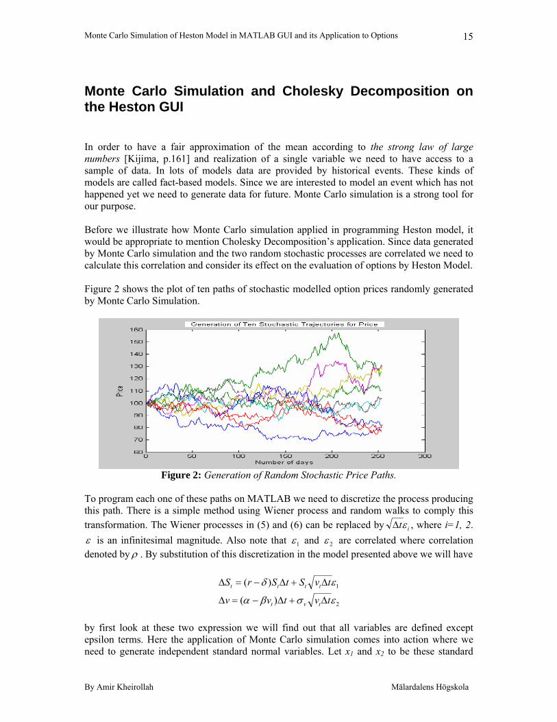
Monte Carlo Simulation and Cholesky Decomposition on the Heston GUI In order to have a fair approximation of the mean according to the strong law of large numbers [Kijima, p.161] and realization of a single variable we need to have access to a sample of data. In lots of models data are provided by historical events. These kinds of models are called fact-based models. Since we are interested to model an event which has not happened yet we need to generate data for future. Monte Carlo simulation is a strong tool for our purpose. Before we illustrate how Monte Carlo simulation applied in programming Heston model, it would be appropriate to mention Cholesky Decomposition’s application. Since data generated by Monte Carlo simulation and the two random stochastic processes are correlated we need to calculate this correlation and consider its effect on the evaluation of options by Heston Model. Figure 2 shows the plot of ten paths of stochastic modelled option prices randomly generated by Monte Carlo Simulation.
Figure 2: Generation of Random Stochastic Price Paths.
To program each one of these paths on MATLAB we need to discretize the process producing this path. There is a simple method using Wiener process and random walks to comply this transformation. The Wiener processes in (5) and (6) can be replaced by itεΔ , where i=1, 2. ε is an infinitesimal magnitude. Also note that 1ε and 2ε are correlated where correlation denoted by ρ . By substitution of this discretization in the model presented above we will have
1)( εδ tvStSrS tttt Δ+Δ−=Δ
2)( εσβα tvtvv tvt Δ+Δ−=Δ by first look at these two expression we will find out that all variables are defined except epsilon terms. Here the application of Monte Carlo simulation comes into action where we need to generate independent standard normal variables. Let x1 and x2 to be these standard

Monte Carlo Simulation of Heston Model in MATLAB GUI and its Application to Options
By Amir Kheirollah Mälardalens Högskola
16
random normal variables with mean zero. If 11 ε=x , then considering statement (11) we will
have 22
12 1 ερρε −+=x [Fink, p.13].
1)( εδ tvStSrS tttt Δ+Δ−=Δ
)1()( 22
1 ερρεσβα −+Δ+Δ−=Δ tvtvv tvt
by this simple transformation epsilon terms are defined. These terms are obtained by Cholesky decomposition. In simple word the multiplication of a random matrix to the correlation matrix decomposed.
Monte Carlo Simulation of Heston Model in MATLAB GUI and its Application to Options
By Amir Kheirollah Mälardalens Högskola
17
Options under Study In this section three underlying options considered by this study and modelled by Heston model under time interval [0,T], which simulated by Monte Carlo simulations are introduced. These three options are most basic and probably most popular options to trade:
1. European Call Option 2. Average Option 3. Lookback Option
In this section each of these options are introduced and some of their characteristics mentioned.
European Call Option
European call option is the basic model for options studied in this paper. It will be followed by this part how the other options introduced here are based on this particular option. European call option can be exercised only on expiration date, considering this characteristic it is the simplest model to simulate by Monte Carlo simulation. If we let S t be the price of the underlying asset at the maturity and K, be the strike price then if S t >K, the investor have the right to buy the asset for the price K and sell it in the market for the price S t and enjoy the differential. Otherwise the investor abandons the right to exercise and do nothing, which in this case his/her loss will be zero. The payoff function in the call case of the European option would be:
{ }+−= KSX t
If we denote the ith realization of ST by its , then the expected payoff from the call option
can be evaluated as
{ }[ ] { }∑=
++ −≈−N
i
itt Ks
NKSE
1
1
for sufficiently large N. We should consider the discount rate in our evaluation of European call option. It let us to have a more precise approximation of the differential.
{ }[ ]+− −= KSEeX trT
Consequently,
{ }∑=
+− −=
N
i
it
rT KsN
eX1
1

Monte Carlo Simulation of Heston Model in MATLAB GUI and its Application to Options
By Amir Kheirollah Mälardalens Högskola
18
Average Option The other option considered in our applet and modelled by the Monte Carlo method in Heston Model is Average or Asian option. Asian option has a payoff that depends on the average value of the underlying asset over some period before expiry. Average options are one of the examples of the path-dependent contracts, because they are not just determined by the value where they reach at the maturity but its value totally depends on the shape of the path during the period as their life-time. The applet written by MATLAB is supposed to estimate the premium of the Average option by Monte Carlo simulation. Let i
ts be the ith realization of S t in the Monte Carlo simulation, then for sufficiently large N we would have,
{ }∑=
+− −=
N
i
it
T KsN
RY1
1
which is an example of ordinary European call option premium written on S(T). In the same way we can obtain ith realization of the Average option. Thus we can estimate the Average option premium in this way,
{ }∑∑=
+=
− −=T
t
it
N
i
T KsTN
RX11
11
One of the advantages of this option is that it reduces the sensitivity of the contract to the price change at the maturity of a contract which is important in the markets which maybe illiquid.
Lookback Option
Lookback option’s payoff is dependent on the maximum or minimum of the asset price achieved during a certain period. The payoff dependent on the underlying price path would cause this derivative to be categorized as a path-dependent security. This maximum or minimum value can be calculated continuously or discretely, Considering a price process {S t }, letting
tTtt SM≤≤
=0max where 0⟩T
then M t is the maximum of the price process during the time interval [ ]T,0 . If the payoff function at maturity is given by
{ }+−= KML t more explicit we can denote it by
{ }[ ]∑=
+
− −=N
i
iT KMN
RLi
1
1τ
Where iτ is the time where the i:th sample has it’s maximum.
Monte Carlo Simulation of Heston Model in MATLAB GUI and its Application to Options
By Amir Kheirollah Mälardalens Högskola
19
Empirical Investigation
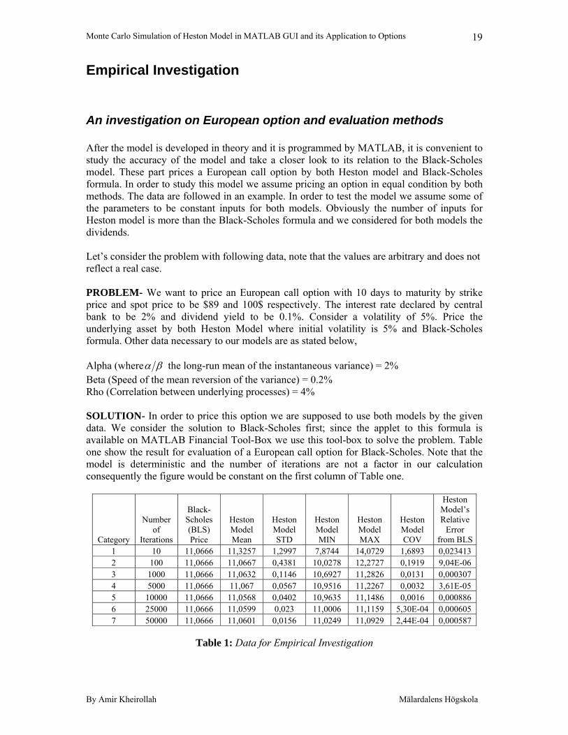
An investigation on European option and evaluation methods After the model is developed in theory and it is programmed by MATLAB, it is convenient to study the accuracy of the model and take a closer look to its relation to the Black-Scholes model. These part prices a European call option by both Heston model and Black-Scholes formula. In order to study this model we assume pricing an option in equal condition by both methods. The data are followed in an example. In order to test the model we assume some of the parameters to be constant inputs for both models. Obviously the number of inputs for Heston model is more than the Black-Scholes formula and we considered for both models the dividends. Let’s consider the problem with following data, note that the values are arbitrary and does not reflect a real case. PROBLEM- We want to price an European call option with 10 days to maturity by strike price and spot price to be $89 and 100$ respectively. The interest rate declared by central bank to be 2% and dividend yield to be 0.1%. Consider a volatility of 5%. Price the underlying asset by both Heston Model where initial volatility is 5% and Black-Scholes formula. Other data necessary to our models are as stated below, Alpha (where βα the long-run mean of the instantaneous variance) = 2% Beta (Speed of the mean reversion of the variance) = 0.2% Rho (Correlation between underlying processes) = 4% SOLUTION- In order to price this option we are supposed to use both models by the given data. We consider the solution to Black-Scholes first; since the applet to this formula is available on MATLAB Financial Tool-Box we use this tool-box to solve the problem. Table one show the result for evaluation of a European call option for Black-Scholes. Note that the model is deterministic and the number of iterations are not a factor in our calculation consequently the figure would be constant on the first column of Table one.
Category
Number of
Iterations
Black-Scholes (BLS) Price
Heston Model Mean
Heston Model STD
Heston Model MIN
Heston Model MAX
Heston Model COV
Heston Model’s Relative
Error from BLS
1 10 11,0666 11,3257 1,2997 7,8744 14,0729 1,6893 0,023413 2 100 11,0666 11,0667 0,4381 10,0278 12,2727 0,1919 9,04E-06 3 1000 11,0666 11,0632 0,1146 10,6927 11,2826 0,0131 0,000307 4 5000 11,0666 11,067 0,0567 10,9516 11,2267 0,0032 3,61E-05 5 10000 11,0666 11,0568 0,0402 10,9635 11,1486 0,0016 0,000886 6 25000 11,0666 11,0599 0,023 11,0006 11,1159 5,30E-04 0,000605 7 50000 11,0666 11,0601 0,0156 11,0249 11,0929 2,44E-04 0,000587
Table 1: Data for Empirical Investigation
Monte Carlo Simulation of Heston Model in MATLAB GUI and its Application to Options
By Amir Kheirollah Mälardalens Högskola
20
Second step on our empirical investigation would be pricing the option by the Heston Model. For this purpose we use the applet written on this model by MATLAB. In order to have fair figures to compare with the result on Black-Scholes seems to be not a strong argument if we run our applet only once for each category. By mathematical statistics we know in order to have a successful hypothesis test we need to have a sample of data and it to be accurate. The probability distribution for a continuous random variable is directly connected to this fact. In order to make our observation more legitimate we have chosen sample of hundred experiments for seven categories of iterations. Since comparison of every single experiment on Heston Model to Black-Scholes formula would not tell a lot about the relationship between this two the mean on Heston Model’s experiment on each categories presented on second column of table one. The data on all experiments is available on appendix. Two observations can be made on this mean values by presenting two simple questions.
1. What is the relation of the mean on stochastic Heston Model to the deterministic Black-Scholes?
2. What the experiments tells us about the accuracy of the Heston formula modelled by Monte Carlo simulation?
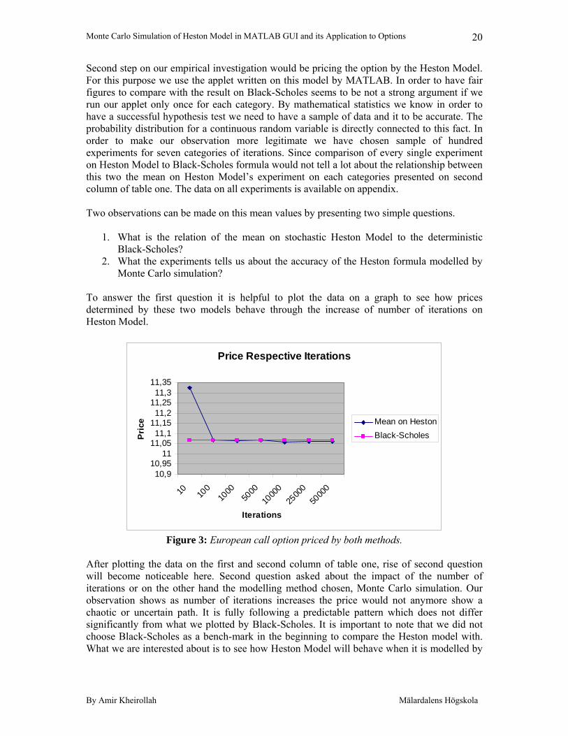
To answer the first question it is helpful to plot the data on a graph to see how prices determined by these two models behave through the increase of number of iterations on Heston Model.
Price Respective Iterations
10,910,95
1111,0511,1
11,1511,2
11,2511,3
11,35
10 100
1000
5000
1000
025
000
5000
0
Iterations
Pric
e Mean on HestonBlack-Scholes
Figure 3: European call option priced by both methods.
After plotting the data on the first and second column of table one, rise of second question will become noticeable here. Second question asked about the impact of the number of iterations or on the other hand the modelling method chosen, Monte Carlo simulation. Our observation shows as number of iterations increases the price would not anymore show a chaotic or uncertain path. It is fully following a predictable pattern which does not differ significantly from what we plotted by Black-Scholes. It is important to note that we did not choose Black-Scholes as a bench-mark in the beginning to compare the Heston model with. What we are interested about is to see how Heston Model will behave when it is modelled by
Monte Carlo Simulation of Heston Model in MATLAB GUI and its Application to Options
By Amir Kheirollah Mälardalens Högskola
21
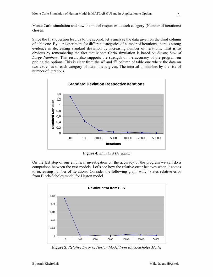
Monte Carlo simulation and how the model responses to each category (Number of iterations) chosen. Since the first question lead us to the second, let’s analyze the data given on the third column of table one. By our experiment for different categories of number of iterations, there is strong evidence in decreasing standard deviation by increasing number of iterations. That is so obvious by remembering the fact that Monte Carlo simulation is based on Strong Law of Large Numbers. This result also supports the strength of the accuracy of the program on pricing the options. This is clear from the 4th and 5th column of table one where the data on two extremes of each category of iterations is given. The interval diminishes by the rise of number of iterations.
Standard Deviation Respective Iterations
0
0,2
0,4
0,6
0,8
1
1,2
1,4
10 100 1000 5000 10000 25000 50000
Iterations
Sta
ndar
d D
evia
tion
Figure 4: Standard Deviation
On the last step of our empirical investigation on the accuracy of the program we can do a comparison between the two models. Let’s see how the relative error behaves when it comes to increasing number of iterations. Consider the following graph which states relative error from Black-Scholes model for Heston model.
Relative error from BLS
0
0,005
0,01
0,015
0,02
0,025
10 100 1000 5000 10000 25000 50000
Figure 5: Relative Error of Heston Model from Black-Scholes Model
Monte Carlo Simulation of Heston Model in MATLAB GUI and its Application to Options
By Amir Kheirollah Mälardalens Högskola
22
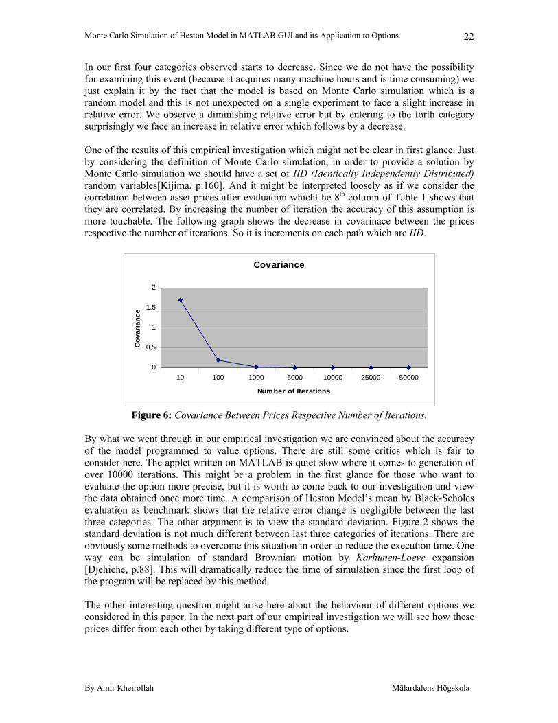
In our first four categories observed starts to decrease. Since we do not have the possibility for examining this event (because it acquires many machine hours and is time consuming) we just explain it by the fact that the model is based on Monte Carlo simulation which is a random model and this is not unexpected on a single experiment to face a slight increase in relative error. We observe a diminishing relative error but by entering to the forth category surprisingly we face an increase in relative error which follows by a decrease. One of the results of this empirical investigation which might not be clear in first glance. Just by considering the definition of Monte Carlo simulation, in order to provide a solution by Monte Carlo simulation we should have a set of IID (Identically Independently Distributed) random variables[Kijima, p.160]. And it might be interpreted loosely as if we consider the correlation between asset prices after evaluation whicht he 8th column of Table 1 shows that they are correlated. By increasing the number of iteration the accuracy of this assumption is more touchable. The following graph shows the decrease in covarinace between the prices respective the number of iterations. So it is increments on each path which are IID.
Covariance
0
0,5
1
1,5
2
10 100 1000 5000 10000 25000 50000
Number of Iterations
Cov
aria
nce
Figure 6: Covariance Between Prices Respective Number of Iterations.
By what we went through in our empirical investigation we are convinced about the accuracy of the model programmed to value options. There are still some critics which is fair to consider here. The applet written on MATLAB is quiet slow where it comes to generation of over 10000 iterations. This might be a problem in the first glance for those who want to evaluate the option more precise, but it is worth to come back to our investigation and view the data obtained once more time. A comparison of Heston Model’s mean by Black-Scholes evaluation as benchmark shows that the relative error change is negligible between the last three categories. The other argument is to view the standard deviation. Figure 2 shows the standard deviation is not much different between last three categories of iterations. There are obviously some methods to overcome this situation in order to reduce the execution time. One way can be simulation of standard Brownian motion by Karhunen-Loeve expansion [Djehiche, p.88]. This will dramatically reduce the time of simulation since the first loop of the program will be replaced by this method. The other interesting question might arise here about the behaviour of different options we considered in this paper. In the next part of our empirical investigation we will see how these prices differ from each other by taking different type of options.
Monte Carlo Simulation of Heston Model in MATLAB GUI and its Application to Options
By Amir Kheirollah Mälardalens Högskola
23
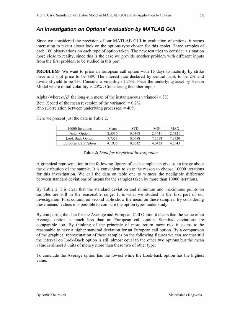
An investigation on Options’ evaluation by MATLAB GUI Since we considered the precision of our MATLAB GUI in evaluation of options, it seems interesting to take a closer look on the options type chosen for this applet. Three samples of each 100 observations on each type of option taken. The new test tries to consider a situation more close to reality, since this is the case we provide another problem with different inputs from the first problem to be studied in this part. PROBLEM- We want to price an European call option with 15 days to maturity by strike price and spot price to be $89. The interest rate declared by central bank to be 2% and dividend yield to be 2%. Consider a volatility of 25%. Price the underlying asset by Heston Model where initial volatility is 25% . Considering the other inputs Alpha (where βα the long-run mean of the instantaneous variance) = 3% Beta (Speed of the mean reversion of the variance) = 0.2% Rho (Correlation between underlying processes) = 40% Here we present just the data in Table 2,
10000 Iterations Mean STD MIN MAX Asian Option 2,5516 0,0368 2,4641 2,6321
Look Back Option 7,7357 0,0688 7,5518 7,8720 European Call Option 4,1935 0,0612 4,0423 4,3343
Table 2: Data for Empirical Investigation
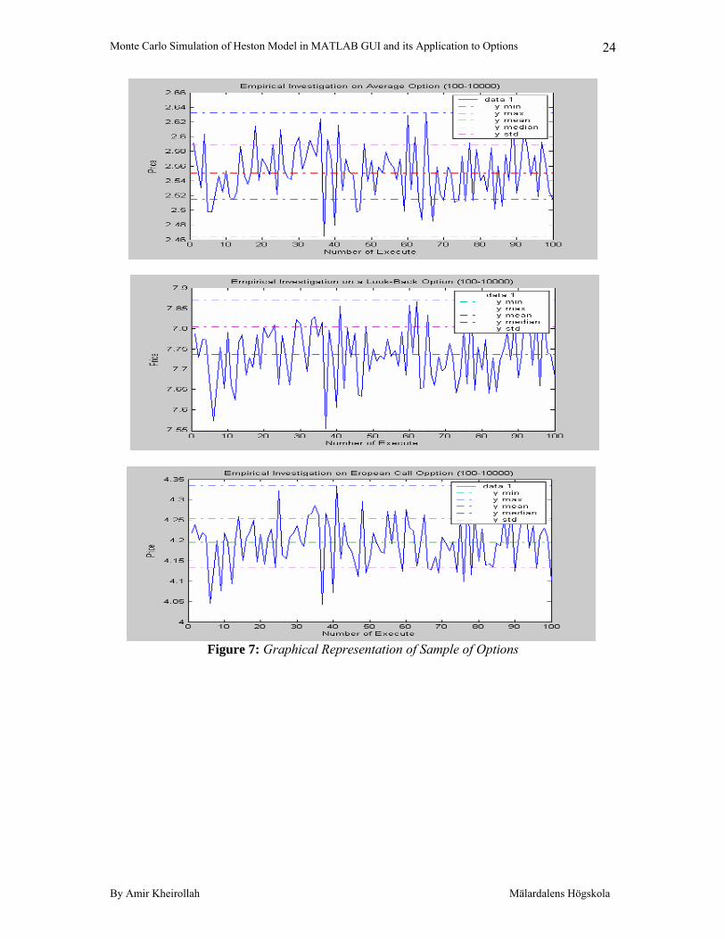
A graphical representation in the following figures of each sample can give us an image about the distribution of the sample. It is convenient to state the reason to choose 10000 iterations for this investigation. We call the data on table one to witness the negligible difference between standard deviations of means for the samples taken by more than 10000 iterations. By Table 2 it is clear that the standard deviation and minimum and maximums points on samples are still in the reasonable range. It is what we studied in the first part of our investigation. First column on second table show the mean on these samples. By considering these means’ values it is possible to compare the option types under study. By comparing the data for the Average and European Call Option it clears that the value of an Average option is much less than an European call option. Standrad deviations are comparable too. By thinking of the principle of more return more risk it seems to be reasonable to have a higher standrad deviation for an European call option. By a comparison of the graphical representation of these samples on the following figures we can see that still the interval on Look-Back option is still almost equal to the other two options but the mean value is almost 3 units of money more than these two of other type. To conclude the Average option has the lowest while the Look-back option has the highest value.
Monte Carlo Simulation of Heston Model in MATLAB GUI and its Application to Options
By Amir Kheirollah Mälardalens Högskola
24
Figure 7: Graphical Representation of Sample of Options
Monte Carlo Simulation of Heston Model in MATLAB GUI and its Application to Options
By Amir Kheirollah Mälardalens Högskola
25
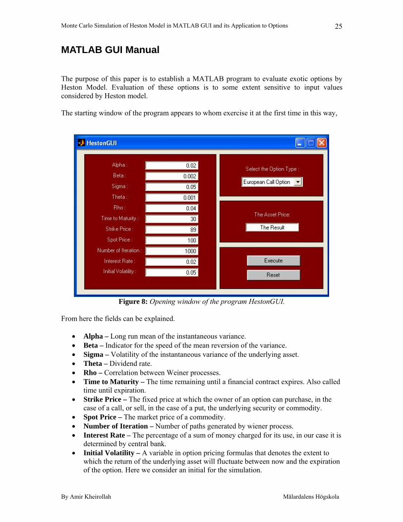
MATLAB GUI Manual The purpose of this paper is to establish a MATLAB program to evaluate exotic options by Heston Model. Evaluation of these options is to some extent sensitive to input values considered by Heston model. The starting window of the program appears to whom exercise it at the first time in this way,
Figure 8: Opening window of the program HestonGUI.
From here the fields can be explained.
• Alpha – Long run mean of the instantaneous variance. • Beta – Indicator for the speed of the mean reversion of the variance. • Sigma – Volatility of the instantaneous variance of the underlying asset. • Theta – Dividend rate. • Rho – Correlation between Weiner processes. • Time to Maturity – The time remaining until a financial contract expires. Also called
time until expiration. • Strike Price – The fixed price at which the owner of an option can purchase, in the
case of a call, or sell, in the case of a put, the underlying security or commodity. • Spot Price – The market price of a commodity. • Number of Iteration – Number of paths generated by wiener process. • Interest Rate – The percentage of a sum of money charged for its use, in our case it is
determined by central bank. • Initial Volatility – A variable in option pricing formulas that denotes the extent to
which the return of the underlying asset will fluctuate between now and the expiration of the option. Here we consider an initial for the simulation.
Monte Carlo Simulation of Heston Model in MATLAB GUI and its Application to Options
By Amir Kheirollah Mälardalens Högskola
26
• Select the Option Type – Make the user capable to evaluate the option by different types.
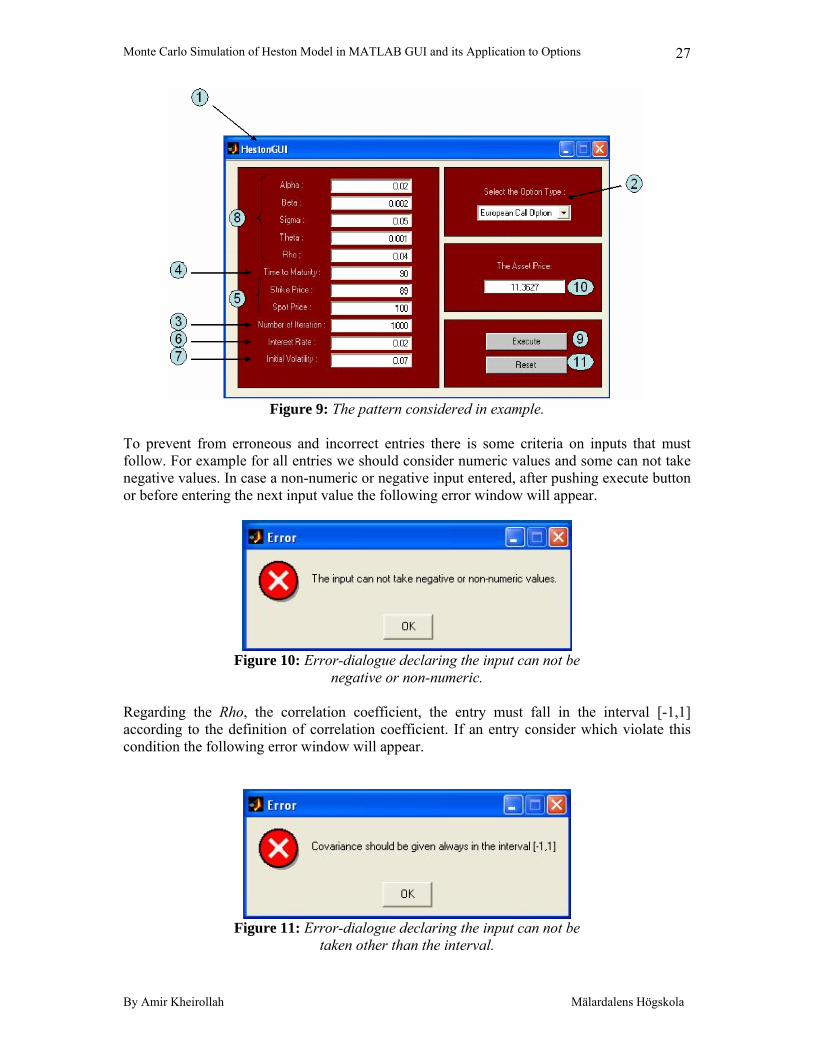
• The Asset Price – The option evaluated amount. • Execute – To run the program. • Reset – To come back to default mode. An example can be helpful to explain how to use the GUI. In this example we will use some of the date pre-entered into the program. The user can follow the following pattern showed on figure 2 to calculate any option values considered in this program.
1- Run the program from MATLAB. 2- Choose the option type you want to calculate its price from the popup menu. In
the case of our example we choose the European option which is by default chosen already by the program.
3- Decide how many iteration you will consider in your calculation. Note that number of iterations can heavily affect on the time of calculations by Monte Carlo simulation. By default the program considers one thousand iterations which we will not change in our example.
4- Put in the length of the period you want to calculate the price for it. The program considers the finance year to be 252 days. In our case we consider a 3 months or 90-days European call option.
5- Next step can be determination of spot and strike price. We will consider the same values taken by default.
6- Interest rate should be considered also as an input to the program. This value usually is declared by central banks in the countries. In our example we consider the interest rate to be 2%.
7- The initial volatility also should be considered. The benchmark for this value can be the historical volatilities in option markets. In our case we consider %7 volatility.
8- The last step in giving data to the program where we put in values for Greeks, we can consider the default values.
9- To see the result we push the execute button and run the program. 10- The result is shown in the asset price field. 11- To reset the program to defaults reset button should be used.
Monte Carlo Simulation of Heston Model in MATLAB GUI and its Application to Options
By Amir Kheirollah Mälardalens Högskola
27
Figure 9: The pattern considered in example.
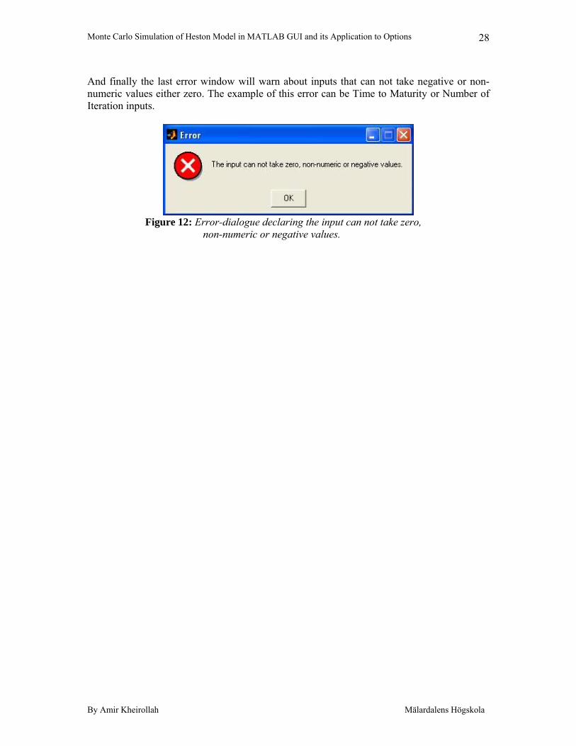
To prevent from erroneous and incorrect entries there is some criteria on inputs that must follow. For example for all entries we should consider numeric values and some can not take negative values. In case a non-numeric or negative input entered, after pushing execute button or before entering the next input value the following error window will appear.
Figure 10: Error-dialogue declaring the input can not be
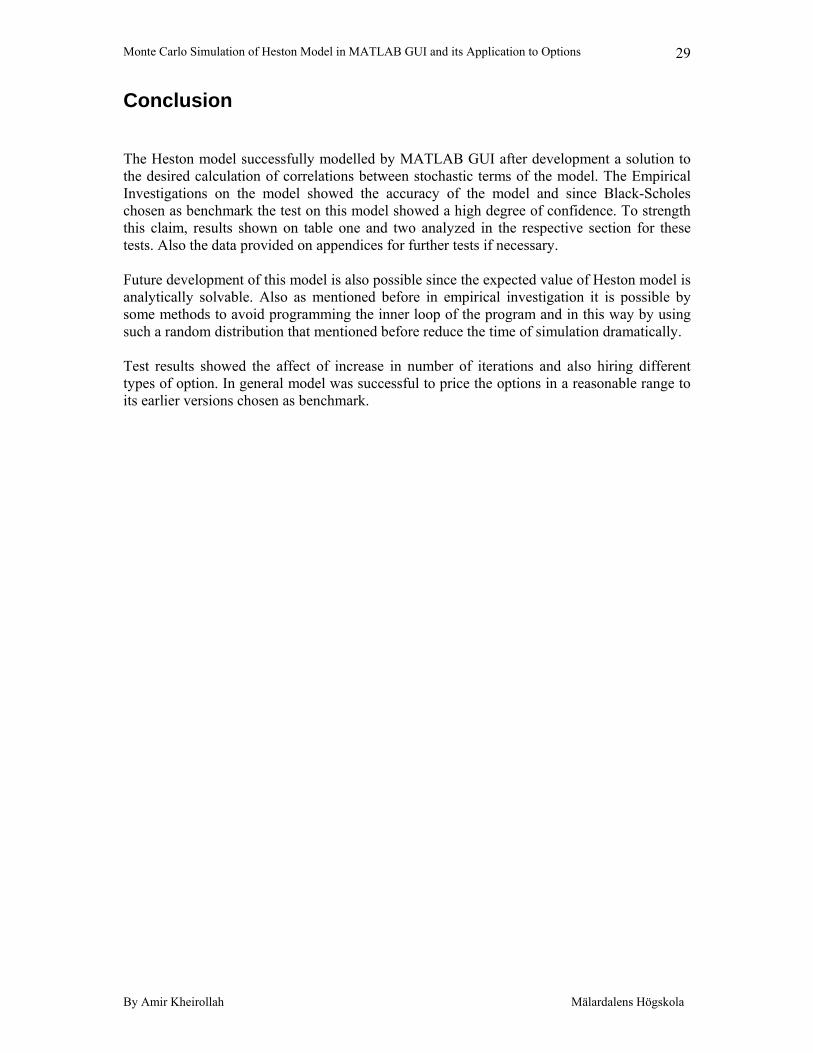
negative or non-numeric. Regarding the Rho, the correlation coefficient, the entry must fall in the interval [-1,1] according to the definition of correlation coefficient. If an entry consider which violate this condition the following error window will appear.
Figure 11: Error-dialogue declaring the input can not be
taken other than the interval.
Monte Carlo Simulation of Heston Model in MATLAB GUI and its Application to Options
By Amir Kheirollah Mälardalens Högskola
28
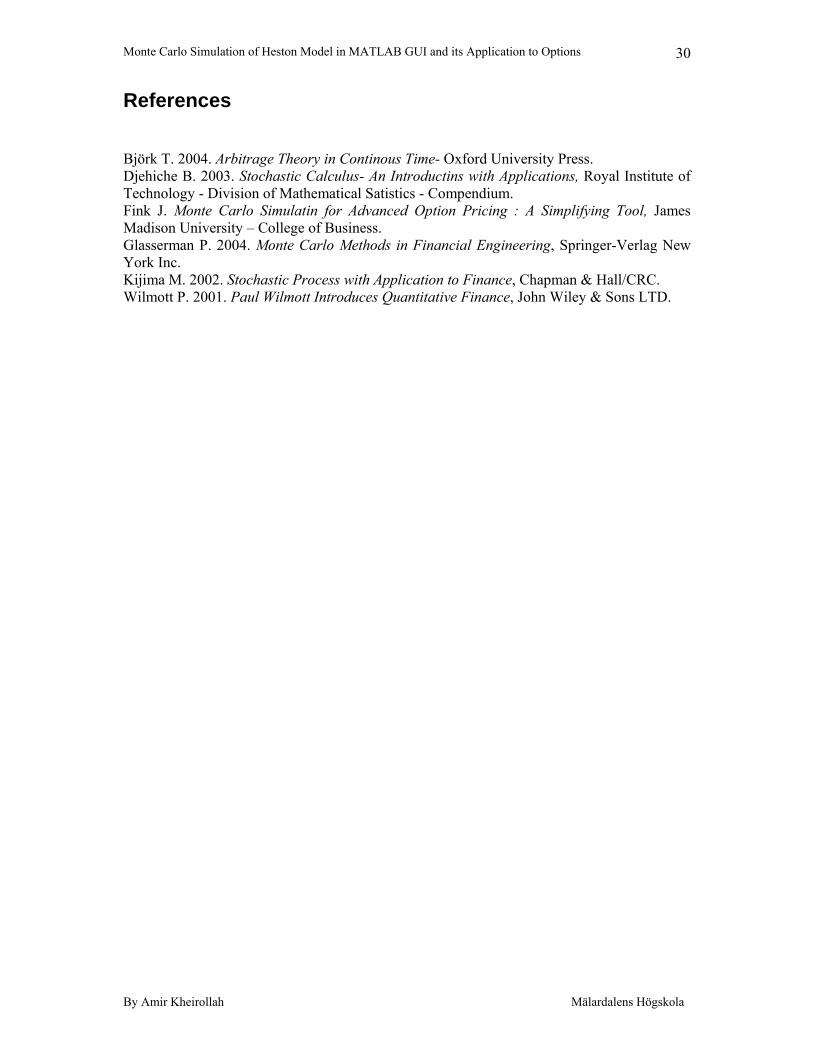
And finally the last error window will warn about inputs that can not take negative or non-numeric values either zero. The example of this error can be Time to Maturity or Number of Iteration inputs.
Figure 12: Error-dialogue declaring the input can not take zero,
non-numeric or negative values.
Monte Carlo Simulation of Heston Model in MATLAB GUI and its Application to Options
By Amir Kheirollah Mälardalens Högskola
29
Conclusion The Heston model successfully modelled by MATLAB GUI after development a solution to the desired calculation of correlations between stochastic terms of the model. The Empirical Investigations on the model showed the accuracy of the model and since Black-Scholes chosen as benchmark the test on this model showed a high degree of confidence. To strength this claim, results shown on table one and two analyzed in the respective section for these tests. Also the data provided on appendices for further tests if necessary. Future development of this model is also possible since the expected value of Heston model is analytically solvable. Also as mentioned before in empirical investigation it is possible by some methods to avoid programming the inner loop of the program and in this way by using such a random distribution that mentioned before reduce the time of simulation dramatically. Test results showed the affect of increase in number of iterations and also hiring different types of option. In general model was successful to price the options in a reasonable range to its earlier versions chosen as benchmark.
Monte Carlo Simulation of Heston Model in MATLAB GUI and its Application to Options
By Amir Kheirollah Mälardalens Högskola
30
References Björk T. 2004. Arbitrage Theory in Continous Time- Oxford University Press. Djehiche B. 2003. Stochastic Calculus- An Introductins with Applications, Royal Institute of Technology - Division of Mathematical Satistics - Compendium. Fink J. Monte Carlo Simulatin for Advanced Option Pricing : A Simplifying Tool, James Madison University – College of Business. Glasserman P. 2004. Monte Carlo Methods in Financial Engineering, Springer-Verlag New York Inc. Kijima M. 2002. Stochastic Process with Application to Finance, Chapman & Hall/CRC. Wilmott P. 2001. Paul Wilmott Introduces Quantitative Finance, John Wiley & Sons LTD.
Monte Carlo Simulation of Heston Model in MATLAB GUI and its Application to Options
By Amir Kheirollah Mälardalens Högskola
31
Appendices
Appendix A
Appendix A-1 function varargout = HestonGUI(varargin) % HESTONGUI M-file for HestonGUI.fig % HESTONGUI, by itself, creates a new HESTONGUI or raises the existing % singleton*. % % H = HESTONGUI returns the handle to a new HESTONGUI or the handle to % the existing singleton*. % % HESTONGUI('CALLBACK',hObject,eventData,handles,...) calls the local % function named CALLBACK in HESTONGUI.M with the given input arguments. % % HESTONGUI('Property','Value',...) creates a new HESTONGUI or raises the % existing singleton*. Starting from the left, property value pairs are % applied to the GUI before HestonGUI_OpeningFunction gets called. An % unrecognized property name or invalid value makes property application % stop. All inputs are passed to HestonGUI_OpeningFcn via varargin. % % *See GUI Options on GUIDE's Tools menu. Choose "GUI allows only one % instance to run (singleton)". % % See also: GUIDE, GUIDATA, GUIHANDLES % Edit the above text to modify the response to help HestonGUI % Last Modified by GUIDE v2.5 05-Mar-2006 18:46:59 % Begin initialization code - DO NOT EDIT gui_Singleton = 1; gui_State = struct('gui_Name', mfilename, ... 'gui_Singleton', gui_Singleton, ... 'gui_OpeningFcn', @HestonGUI_OpeningFcn, ... 'gui_OutputFcn', @HestonGUI_OutputFcn, ... 'gui_LayoutFcn', [] , ... 'gui_Callback', []); if nargin & isstr(varargin{1}) gui_State.gui_Callback = str2func(varargin{1}); end if nargout [varargout{1:nargout}] = gui_mainfcn(gui_State, varargin{:}); else gui_mainfcn(gui_State, varargin{:}); end % End initialization code - DO NOT EDIT % --- Executes just before HestonGUI is made visible. function HestonGUI_OpeningFcn(hObject, eventdata, handles, varargin) % This function has no output args, see OutputFcn. % hObject handle to figure % eventdata reserved - to be defined in a future version of MATLAB
Monte Carlo Simulation of Heston Model in MATLAB GUI and its Application to Options
By Amir Kheirollah Mälardalens Högskola
32
% handles structure with handles and user data (see GUIDATA) % varargin command line arguments to HestonGUI (see VARARGIN) % Choose default command line output for HestonGUI handles.output = hObject; %-------------------------Initializing Values------------------------ handles.alpha = 0.02; set(handles.Alpha, 'String', '0.02'); handles.beta = 0.002; set(handles.Beta, 'String', '0.002'); handles.sigma = 0.05; set(handles.Sigma, 'String', '0.05'); handles.theta = 0.001; set(handles.Theta, 'String', '0.001'); handles.rho = 0.04; set(handles.Rho, 'String', '0.04'); handles.t = 30; set(handles.T, 'String', '30'); handles.strike = 89; set(handles.Strike, 'String', '89'); handles.spot = 100; set(handles.Spot, 'String', '100'); handles.max1 = 1000; set(handles.Max1, 'String', '1000'); handles.r = 0.02; set(handles.R, 'String', '0.02'); handles.v0 = 0.05; set(handles.V0, 'String', '0.05'); handles.optionType = 1; handles.chooser = true; %set(handle.optionType1, 'Enable', 'on'); %set(handles.optionType1, 'BackgroundColor', 'white'); %set(handle.optionType2, 'Enable', 'on'); %set(handles.optionType2, 'BackgroundColor', 'white'); %set(handle.optionType3, 'Enable', 'on'); %set(handles.optionType3, 'BackgroundColor', 'white'); % Update handles structure guidata(hObject, handles); % UIWAIT makes HestonGUI wait for user response (see UIRESUME) % uiwait(handles.figure1); % --- Outputs from this function are returned to the command line. function varargout = HestonGUI_OutputFcn(hObject, eventdata, handles) % varargout cell array for returning output args (see VARARGOUT); % hObject handle to figure % eventdata reserved - to be defined in a future version of MATLAB % handles structure with handles and user data (see GUIDATA) % Get default command line output from handles structure varargout{1} = handles.output;
Monte Carlo Simulation of Heston Model in MATLAB GUI and its Application to Options
By Amir Kheirollah Mälardalens Högskola
33
%------------------- End of Initializing Values------------------------ %-------------------------- Saves the inputs ------------------------ % --- Executes during object creation, after setting all properties. function Alpha_CreateFcn(hObject, eventdata, handles) % hObject handle to Alpha (see GCBO) % eventdata reserved - to be defined in a future version of MATLAB % handles empty - handles not created until after all CreateFcns called % Hint: edit controls usually have a white background on Windows. % See ISPC and COMPUTER. if ispc set(hObject,'BackgroundColor','white'); else set(hObject,'BackgroundColor',get(0,'defaultUicontrolBackgroundColor')); end function Alpha_Callback(hObject, eventdata, handles) % hObject handle to Alpha (see GCBO) % eventdata reserved - to be defined in a future version of MATLAB % handles structure with handles and user data (see GUIDATA) % Hints: get(hObject,'String') returns contents of Alpha as text % str2double(get(hObject,'String')) returns contents of Alpha as a double %--- returns contents of Alpha as a double entry = str2double(get(hObject,'String')); if isnumeric(entry)& entry >= 0 %its ok handles.alpha = entry; %copy variable guidata(hObject,handles); %save changes else errordlg('The input can not take negative or non-numeric values.','Error');% show error message for anything else end set(hObject,'String',num2str(handles.alpha)); %return old value of stock price % --- Executes during object creation, after setting all properties. function Beta_CreateFcn(hObject, eventdata, handles) % hObject handle to Beta (see GCBO) % eventdata reserved - to be defined in a future version of MATLAB % handles empty - handles not created until after all CreateFcns called % Hint: edit controls usually have a white background on Windows. % See ISPC and COMPUTER. if ispc set(hObject,'BackgroundColor','white'); else set(hObject,'BackgroundColor',get(0,'defaultUicontrolBackgroundColor')); end function Beta_Callback(hObject, eventdata, handles) % hObject handle to Beta (see GCBO) % eventdata reserved - to be defined in a future version of MATLAB % handles structure with handles and user data (see GUIDATA)
Monte Carlo Simulation of Heston Model in MATLAB GUI and its Application to Options
By Amir Kheirollah Mälardalens Högskola
34
% Hints: get(hObject,'String') returns contents of Beta as text % str2double(get(hObject,'String')) returns contents of Beta as a double %--- returns contents of Beta as a double entry = str2double(get(hObject,'String')); if isnumeric(entry)& entry >=0 %its ok handles.beta = entry; %copy variable guidata(hObject,handles); %save changes else errordlg('The input can not take negative or non-numeric values.','Error');% show error message for anything else end set(hObject,'String',num2str(handles.beta)); %return old value of stock price % --- Executes during object creation, after setting all properties. function Sigma_CreateFcn(hObject, eventdata, handles) % hObject handle to Sigma (see GCBO) % eventdata reserved - to be defined in a future version of MATLAB % handles empty - handles not created until after all CreateFcns called % Hint: edit controls usually have a white background on Windows. % See ISPC and COMPUTER. if ispc set(hObject,'BackgroundColor','white'); else set(hObject,'BackgroundColor',get(0,'defaultUicontrolBackgroundColor')); end function Sigma_Callback(hObject, eventdata, handles) % hObject handle to Sigma (see GCBO) % eventdata reserved - to be defined in a future version of MATLAB % handles structure with handles and user data (see GUIDATA) % Hints: get(hObject,'String') returns contents of Sigma as text % str2double(get(hObject,'String')) returns contents of Sigma as a double %--- returns contents of Sigma as a double entry = str2double(get(hObject,'String')); if isnumeric(entry)& entry >=0 %its ok handles.sigma = entry; %copy variable guidata(hObject,handles); %save changes else errordlg('The input can not take negative or non-numeric values.','Error');% show error message for anything else end set(hObject,'String',num2str(handles.sigma)); %return old value of stock price % --- Executes during object creation, after setting all properties. function Theta_CreateFcn(hObject, eventdata, handles) % hObject handle to Theta (see GCBO) % eventdata reserved - to be defined in a future version of MATLAB % handles empty - handles not created until after all CreateFcns called % Hint: edit controls usually have a white background on Windows.
Monte Carlo Simulation of Heston Model in MATLAB GUI and its Application to Options
By Amir Kheirollah Mälardalens Högskola
35
% See ISPC and COMPUTER. if ispc set(hObject,'BackgroundColor','white'); else set(hObject,'BackgroundColor',get(0,'defaultUicontrolBackgroundColor')); end function Theta_Callback(hObject, eventdata, handles) % hObject handle to Theta (see GCBO) % eventdata reserved - to be defined in a future version of MATLAB % handles structure with handles and user data (see GUIDATA) % Hints: get(hObject,'String') returns contents of Theta as text % str2double(get(hObject,'String')) returns contents of Theta as a double %--- returns contents of Theta as a double entry = str2double(get(hObject,'String')); if isnumeric(entry)& entry >=0 %its ok handles.theta = entry; %copy variable guidata(hObject,handles); %save changes else errordlg('The input can not take negative or non-numeric values.','Error');% show error message for anything else end set(hObject,'String',num2str(handles.theta)); %return old value of stock price % --- Executes during object creation, after setting all properties. function Rho_CreateFcn(hObject, eventdata, handles) % hObject handle to Rho (see GCBO) % eventdata reserved - to be defined in a future version of MATLAB % handles empty - handles not created until after all CreateFcns called % Hint: edit controls usually have a white background on Windows. % See ISPC and COMPUTER. if ispc set(hObject,'BackgroundColor','white'); else set(hObject,'BackgroundColor',get(0,'defaultUicontrolBackgroundColor')); end function Rho_Callback(hObject, eventdata, handles) % hObject handle to Rho (see GCBO) % eventdata reserved - to be defined in a future version of MATLAB % handles structure with handles and user data (see GUIDATA) % Hints: get(hObject,'String') returns contents of Rho as text % str2double(get(hObject,'String')) returns contents of Rho as a double %--- returns contents of Rho as a double entry = str2double(get(hObject,'String')); if isnumeric(entry)& entry >-1 & entry <1 %its ok handles.rho = entry; %copy variable guidata(hObject,handles); %save changes else
Monte Carlo Simulation of Heston Model in MATLAB GUI and its Application to Options
By Amir Kheirollah Mälardalens Högskola
36
errordlg('Covariance should be given always in the interval [-1,1]','Error');% show error message for anything else end set(hObject,'String',num2str(handles.rho)); %return old value of stock price % --- Executes during object creation, after setting all properties. function T_CreateFcn(hObject, eventdata, handles) % hObject handle to T (see GCBO) % eventdata reserved - to be defined in a future version of MATLAB % handles empty - handles not created until after all CreateFcns called % Hint: edit controls usually have a white background on Windows. % See ISPC and COMPUTER. if ispc set(hObject,'BackgroundColor','white'); else set(hObject,'BackgroundColor',get(0,'defaultUicontrolBackgroundColor')); end function T_Callback(hObject, eventdata, handles) % hObject handle to T (see GCBO) % eventdata reserved - to be defined in a future version of MATLAB % handles structure with handles and user data (see GUIDATA) % Hints: get(hObject,'String') returns contents of T as text % str2double(get(hObject,'String')) returns contents of T as a double %--- returns contents of T as a double entry = str2double(get(hObject,'String')); if isnumeric(entry)& entry >0 %its ok handles.t = entry; %copy variable guidata(hObject,handles); %save changes else errordlg('The input can not take zero, non-numeric or negative values.','Error');% show error message for anything else end set(hObject,'String',num2str(handles.t)); %return old value of stock price % --- Executes during object creation, after setting all properties. function Strike_CreateFcn(hObject, eventdata, handles) % hObject handle to Strike (see GCBO) % eventdata reserved - to be defined in a future version of MATLAB % handles empty - handles not created until after all CreateFcns called % Hint: edit controls usually have a white background on Windows. % See ISPC and COMPUTER. if ispc set(hObject,'BackgroundColor','white'); else set(hObject,'BackgroundColor',get(0,'defaultUicontrolBackgroundColor')); end function Strike_Callback(hObject, eventdata, handles) % hObject handle to Strike (see GCBO) % eventdata reserved - to be defined in a future version of MATLAB
Monte Carlo Simulation of Heston Model in MATLAB GUI and its Application to Options
By Amir Kheirollah Mälardalens Högskola
37
% handles structure with handles and user data (see GUIDATA) % Hints: get(hObject,'String') returns contents of Strike as text % str2double(get(hObject,'String')) returns contents of Strike as a double %--- returns contents of Strike Price as a double entry = str2double(get(hObject,'String')); if isnumeric(entry)& entry >0 %its ok handles.strike = entry; %copy variable guidata(hObject,handles); %save changes else errordlg('The input can not take zero, non-numeric or negative values.','Error');% show error message for anything else end set(hObject,'String',num2str(handles.strike)); %return old value of stock price % --- Executes during object creation, after setting all properties. function Spot_CreateFcn(hObject, eventdata, handles) % hObject handle to Spot (see GCBO) % eventdata reserved - to be defined in a future version of MATLAB % handles empty - handles not created until after all CreateFcns called % Hint: edit controls usually have a white background on Windows. % See ISPC and COMPUTER. if ispc set(hObject,'BackgroundColor','white'); else set(hObject,'BackgroundColor',get(0,'defaultUicontrolBackgroundColor')); end function Spot_Callback(hObject, eventdata, handles) % hObject handle to Spot (see GCBO) % eventdata reserved - to be defined in a future version of MATLAB % handles structure with handles and user data (see GUIDATA) % Hints: get(hObject,'String') returns contents of Spot as text % str2double(get(hObject,'String')) returns contents of Spot as a double %--- returns contents of Strike Price as a double entry = str2double(get(hObject,'String')); if isnumeric(entry)& entry >0 %its ok handles.spot = entry; %copy variable guidata(hObject,handles); %save changes else errordlg('The input can not take zero, non-numeric or negative values.','Error');% show error message for anything else end set(hObject,'String',num2str(handles.spot)); %return old value of stock price % --- Executes during object creation, after setting all properties. function Max1_CreateFcn(hObject, eventdata, handles) % hObject handle to Max1 (see GCBO) % eventdata reserved - to be defined in a future version of MATLAB % handles empty - handles not created until after all CreateFcns called % Hint: edit controls usually have a white background on Windows. % See ISPC and COMPUTER.
Monte Carlo Simulation of Heston Model in MATLAB GUI and its Application to Options
By Amir Kheirollah Mälardalens Högskola
38
if ispc set(hObject,'BackgroundColor','white'); else set(hObject,'BackgroundColor',get(0,'defaultUicontrolBackgroundColor')); end function Max1_Callback(hObject, eventdata, handles) % hObject handle to Max1 (see GCBO) % eventdata reserved - to be defined in a future version of MATLAB % handles structure with handles and user data (see GUIDATA) % Hints: get(hObject,'String') returns contents of Max1 as text % str2double(get(hObject,'String')) returns contents of Max1 as a double %--- returns contents of iterations as a double entry = str2double(get(hObject,'String')); if isnumeric(entry)& entry >0 %its ok handles.max1 = entry; %copy variable guidata(hObject,handles); %save changes else errordlg('The input can not take zero, non-numeric or negative values.','Error');% show error message for anything else end set(hObject,'String',num2str(handles.max1)); %return old value of stock price % --- Executes during object creation, after setting all properties. function R_CreateFcn(hObject, eventdata, handles) % hObject handle to R (see GCBO) % eventdata reserved - to be defined in a future version of MATLAB % handles empty - handles not created until after all CreateFcns called % Hint: edit controls usually have a white background on Windows. % See ISPC and COMPUTER. if ispc set(hObject,'BackgroundColor','white'); else set(hObject,'BackgroundColor',get(0,'defaultUicontrolBackgroundColor')); end function R_Callback(hObject, eventdata, handles) % hObject handle to R (see GCBO) % eventdata reserved - to be defined in a future version of MATLAB % handles structure with handles and user data (see GUIDATA) % Hints: get(hObject,'String') returns contents of R as text % str2double(get(hObject,'String')) returns contents of R as a double %--- returns contents of interest rate as a double entry = str2double(get(hObject,'String')); if isnumeric(entry)& entry >=0 %its ok, consider the fact that interest rate can take negative form in wiered stuations of the market. handles.r = entry; %copy variable guidata(hObject,handles); %save changes else
Monte Carlo Simulation of Heston Model in MATLAB GUI and its Application to Options
By Amir Kheirollah Mälardalens Högskola
39
errordlg('The input can not take non-numeric or negative values.','Error');% show error message for anything else end set(hObject,'String',num2str(handles.r)); %return old value of stock price % --- Executes during object creation, after setting all properties. function V0_CreateFcn(hObject, eventdata, handles) % hObject handle to V0 (see GCBO) % eventdata reserved - to be defined in a future version of MATLAB % handles empty - handles not created until after all CreateFcns called % Hint: edit controls usually have a white background on Windows. % See ISPC and COMPUTER. if ispc set(hObject,'BackgroundColor','white'); else set(hObject,'BackgroundColor',get(0,'defaultUicontrolBackgroundColor')); end function V0_Callback(hObject, eventdata, handles) % hObject handle to V0 (see GCBO) % eventdata reserved - to be defined in a future version of MATLAB % handles structure with handles and user data (see GUIDATA) % Hints: get(hObject,'String') returns contents of V0 as text % str2double(get(hObject,'String')) returns contents of V0 as a double %--- returns contents of initial volatility as a double entry = str2double(get(hObject,'String')); if isnumeric(entry)& entry >=0 %its ok handles.v0 = entry; %copy variable guidata(hObject,handles); %save changes else errordlg('The input can not take non-numeric or negative values.','Error');% show error message for anything else end set(hObject,'String',num2str(handles.v0)); %return old value of stock price %-------------- End of Handling Inputs ---------------------------- % --- Executes during object creation, after setting all properties. function Print_Result_CreateFcn(hObject, eventdata, handles) % hObject handle to Print_Result (see GCBO) % eventdata reserved - to be defined in a future version of MATLAB % handles empty - handles not created until after all CreateFcns called % Hint: edit controls usually have a white background on Windows.
Monte Carlo Simulation of Heston Model in MATLAB GUI and its Application to Options
By Amir Kheirollah Mälardalens Högskola
40
% See ISPC and COMPUTER. if ispc set(hObject,'BackgroundColor','white'); else set(hObject,'BackgroundColor',get(0,'defaultUicontrolBackgroundColor')); end function Print_Result_Callback(hObject, eventdata, handles) % hObject handle to Print_Result (see GCBO) % eventdata reserved - to be defined in a future version of MATLAB % handles structure with handles and user data (see GUIDATA) % Hints: get(hObject,'String') returns contents of Print_Result as text % str2double(get(hObject,'String')) returns contents of Print_Result as a double % --- Executes during object creation, after setting all properties. function optionType_CreateFcn(hObject, eventdata, handles) % hObject handle to optionType (see GCBO) % eventdata reserved - to be defined in a future version of MATLAB % handles empty - handles not created until after all CreateFcns called % Hint: popupmenu controls usually have a white background on Windows. % See ISPC and COMPUTER. if ispc set(hObject,'BackgroundColor','white'); else set(hObject,'BackgroundColor',get(0,'defaultUicontrolBackgroundColor')); end % --- Executes on selection change in optionType. function optionType_Callback(hObject, eventdata, handles) % hObject handle to optionType (see GCBO) % eventdata reserved - to be defined in a future version of MATLAB % handles structure with handles and user data (see GUIDATA) % Hints: contents = get(hObject,'String') returns optionType contents as cell array % contents{get(hObject,'Value')} returns selected item from optionType handles.optionType = get(hObject, 'Value'); guidata(hObject, handles); val=handles.optionType; %set(handle.optionType1, 'Enable', 'on'); %set(handles.optionType1, 'BackgroundColor', 'white'); %set(handle.optionType2, 'Enable', 'on'); %set(handles.optionType2, 'BackgroundColor', 'white'); %set(handle.optionType3, 'Enable', 'on'); %set(handles.optionType3, 'BackgroundColor', 'white'); % --- Executes on button press in Execute. function Execute_Callback(hObject, eventdata, handles) % hObject handle to Execute (see GCBO) % eventdata reserved - to be defined in a future version of MATLAB % handles structure with handles and user data (see GUIDATA)
Monte Carlo Simulation of Heston Model in MATLAB GUI and its Application to Options
By Amir Kheirollah Mälardalens Högskola
41
%--------------------- Calculating The results ----------------------- handles.optionType switch handles.optionType case 1 % write code for European option [EU,EUfinal,s] = europeanoption(handles.alpha,... handles.beta,... % and so on handles.sigma,... handles.theta,... handles.rho,... handles.t,... handles.r,... handles.max1,... handles.spot,... handles.v0,... handles.strike); % show result set(handles.Print_Result,'String',num2str(EUfinal)); case 2 % write code for Asian option [AS,ASfinal,s] = asianoption(handles.alpha,... handles.beta,... % and so on handles.sigma,... handles.theta,... handles.rho,... handles.t,... handles.r,... handles.max1,... handles.spot,... handles.v0,... handles.strike); % show result set(handles.Print_Result,'String',num2str(ASfinal)); case 3 % write code for Lookback option [LB,LBfinal,s] = lookback(handles.alpha,... handles.beta,... % and so on handles.sigma,... handles.theta,... handles.rho,... handles.t,... handles.r,... handles.max1,... handles.spot,... handles.v0,... handles.strike); % show result set(handles.Print_Result,'String',num2str(LBfinal)); end %--------------------- End of Switching and Printing the results -------------------------- % --- Executes on button press in Reset. function Reset_Callback(hObject, eventdata, handles) % hObject handle to Reset (see GCBO) % eventdata reserved - to be defined in a future version of MATLAB
Monte Carlo Simulation of Heston Model in MATLAB GUI and its Application to Options
By Amir Kheirollah Mälardalens Högskola
42
% handles structure with handles and user data (see GUIDATA) %-------------------- Reset the initial values ------------------ handles.alpha = 0.02; set(handles.Alpha, 'String', '0.02'); handles.beta = 0.002; set(handles.Beta, 'String', '0.002'); handles.sigma = 0.05; set(handles.Sigma, 'String', '0.05'); handles.theta = 0.001; set(handles.Theta, 'String', '0.001'); handles.rho = 0.04; set(handles.Rho, 'String', '0.04'); handles.t = 30; set(handles.T, 'String', '30'); handles.strike = 89; set(handles.Strike, 'String', '89'); handles.spot = 100; set(handles.Spot, 'String', '100'); handles.max1 = 1000; set(handles.Max1, 'String', '1000'); handles.r = 0.02; set(handles.R, 'String', '0.02'); handles.v0 = 0.05; set(handles.V0, 'String', '0.05'); handles.optionType = 1; handles.chooser = true; % -------------------------------------------------------------------- function File_Callback(hObject, eventdata, handles) % hObject handle to File (see GCBO) % eventdata reserved - to be defined in a future version of MATLAB % handles structure with handles and user data (see GUIDATA) % -------------------------------------------------------------------- function Open_Callback(hObject, eventdata, handles) % hObject handle to Open (see GCBO) % eventdata reserved - to be defined in a future version of MATLAB % handles structure with handles and user data (see GUIDATA) % -------------------------------------------------------------------- function Save_Callback(hObject, eventdata, handles) % hObject handle to Save (see GCBO) % eventdata reserved - to be defined in a future version of MATLAB % handles structure with handles and user data (see GUIDATA) % -------------------------------------------------------------------- function Exit_Callback(hObject, eventdata, handles) % hObject handle to Exit (see GCBO) % eventdata reserved - to be defined in a future version of MATLAB % handles structure with handles and user data (see GUIDATA) % --------------------------------------------------------------------
Monte Carlo Simulation of Heston Model in MATLAB GUI and its Application to Options
By Amir Kheirollah Mälardalens Högskola
43
function Edit_Callback(hObject, eventdata, handles) % hObject handle to Edit (see GCBO) % eventdata reserved - to be defined in a future version of MATLAB % handles structure with handles and user data (see GUIDATA) % -------------------------------------------------------------------- function Help_Callback(hObject, eventdata, handles) % hObject handle to Help (see GCBO) % eventdata reserved - to be defined in a future version of MATLAB % handles structure with handles and user data (see GUIDATA) % -------------------------------------------------------------------- function Manual_Callback(hObject, eventdata, handles) % hObject handle to Manual (see GCBO) % eventdata reserved - to be defined in a future version of MATLAB % handles structure with handles and user data (see GUIDATA) % -------------------------------------------------------------------- function About_Callback(hObject, eventdata, handles) % hObject handle to About (see GCBO) % eventdata reserved - to be defined in a future version of MATLAB % handles structure with handles and user data (see GUIDATA) % -------------------------------------------------------------------- function Untitled_1_Callback(hObject, eventdata, handles) % hObject handle to Untitled_1 (see GCBO) % eventdata reserved - to be defined in a future version of MATLAB % handles structure with handles and user data (see GUIDATA) % -------------------------------------------------------------------- function Untitled_2_Callback(hObject, eventdata, handles) % hObject handle to Untitled_2 (see GCBO) % eventdata reserved - to be defined in a future version of MATLAB % handles structure with handles and user data (see GUIDATA) % -------------------------------------------------------------------- function MFile_Callback(hObject, eventdata, handles) % hObject handle to MFile (see GCBO) % eventdata reserved - to be defined in a future version of MATLAB % handles structure with handles and user data (see GUIDATA) % --- Executes on button press in Heston_Model. function Heston_Model_Callback(hObject, eventdata, handles) % hObject handle to Heston_Model (see GCBO) % eventdata reserved - to be defined in a future version of MATLAB % handles structure with handles and user data (see GUIDATA) % Hint: get(hObject,'Value') returns toggle state of Heston_Model % --- Executes on button press in Black_Scholes_Model. function Black_Scholes_Model_Callback(hObject, eventdata, handles) % hObject handle to Black_Scholes_Model (see GCBO)
Monte Carlo Simulation of Heston Model in MATLAB GUI and its Application to Options
By Amir Kheirollah Mälardalens Högskola
44
% eventdata reserved - to be defined in a future version of MATLAB % handles structure with handles and user data (see GUIDATA) % Hint: get(hObject,'Value') returns toggle state of Black_Scholes_Model % --- If Enable == 'on', executes on mouse press in 5 pixel border. % --- Otherwise, executes on mouse press in 5 pixel border or over Print_Result. function Print_Result_ButtonDownFcn(hObject, eventdata, handles) % hObject handle to Print_Result (see GCBO) % eventdata reserved - to be defined in a future version of MATLAB % handles structure with handles and user data (see GUIDATA)
Appendix A-2 function [epsilon,s,v] = heston23(alpha,beta,sigma,theta,rho,t,r,spot,v0) % [epsilon s v] = heston23(alpha,beta,sigma,theta,rho,t,r,max1,spot,v0) % function [epsilon,s,v] = heston2(alpha,beta,sigma,theta,rho,T,r,max1) % The heston function calculates the asset price and its volatility % epsilon : the component of replacement of Wiener process in order to % discretization of GBM. By using sholesky decomposition the correlation % between these two valaues, epsilon one and two, is calculated. % s : asset price at maturity % v : volatility or instantanous variance % alpha : a component of long-run mean of instantanous variance % beta : indicator for the speed of mean-reversion of instantanous % variance % sigma : volatility of volatility % theta : the dividend yield % rho : correlation between two Wiener processes discussed in epsilon % determination earlier % T : time to maturity considered in days % r : interest rate % max1 : is the maximum number of iteration % File : Heston.m % Description : Heston Model Simulation by Monte Carlo and its Application % to Exotic Options % Author : Amir Kheirollah % Mail : [email protected] %---------------------------------------------------------------------- % max1 = 100; % alpha = 0.01; % beta = 0.001; % sigma = 0.075; % theta = 0.001; % rho = 0.04; % t = 90; % r = 0.02; s(1) = spot; v(1) = v0; M = [1 rho; rho 1]; % The diagonal matrix for use in cholesky method if (nargin == 9) % the same problem here with nargin. for i=2:(t+2)

Monte Carlo Simulation of Heston Model in MATLAB GUI and its Application to Options
By Amir Kheirollah Mälardalens Högskola
45
epsilon = chol(M)'*randn(2,1); % Generates random numbers in order to determine epsilons by use of %cholesky method deltatime =1/252; % time discretization over the life of the option' the time step length is % one day. v(i) = v(i-1) + [ alpha - beta * v(i-1)] * deltatime + sigma * [[v(i-1) * deltatime]^.5] * epsilon(2); s(i) = s(i-1) + (r- theta) * s(i-1) * deltatime + s(i-1) * [[v(i-1) * deltatime]^.5] * epsilon(1); end else disp('The number of inputs exceed the functions inputs number'); end
Appendix A-3 function [endValues,average,s] = heston4(alpha,beta,sigma,theta,rho,t,r,max1,spot,v0) % [endValues,average,s]=heston4(0.02,0.002,0.001,0.01,0.04,365,0.02,10,100,0.05) % heston4(0.02,0.002,0.001,0.01,0.04,365,0.02,10,100,0.05) if (nargin == 10) for j=1:max1 % The loop generating trajectories essential to Monte Carlo Simulation set(0,'RecursionLimit',100); [epsilon,s(j,:),v]=heston23(alpha,beta,sigma,theta,rho,t,r,spot,v0);%HÄRANROPAR DU Heston23.m average(j) = mean(s(j,:)); % calculate the mean endValues(j)=s(j,t); end else disp('The number of inputs exceed the functions inputs number'); end %figure; %plot(1:252+2,s)
Appendix A-4 function [AS,ASfinal,s] = asianoption(alpha,beta,sigma,theta,rho,t,r,max1,spot,v0,strike) % [a b c]=asianoption(0.02,0.002,0.001,0.01,0.04,365,0.02,10,100,0.05,100) % asianoption(0.02,0.002,0.001,0.01,0.04,365,0.02,10,100,0.05,100) %disp('ASIAN'); if (nargin == 11) % The loop generating trajectories essential to Monte Carlo Simulation set(0,'RecursionLimit',100); %[average,s] = heston4(alpha,beta,sigma,theta,rho,T,r,max1,s0,v0); [endValues,AS,s] = heston4(alpha,beta,sigma,theta,rho,t,r,max1,spot,v0); else disp('The number of inputs exceed the functions inputs number'); end ASfinal = exp(-r*(t/252))*mean(max((AS)-strike,0)); function [endValues,LBfinal,s] = lookback(alpha,beta,sigma,theta,rho,t,r,max1,spot,v0,strike) % [a b c]=lookback(0.02,0.002,0.001,0.01,0.04,365,0.02,10,100,0.05,100) % lookback(0.02,0.002,0.001,0.01,0.04,365,0.02,10,100,0.05,100) %disp('LB'); if (nargin == 11)
Monte Carlo Simulation of Heston Model in MATLAB GUI and its Application to Options
By Amir Kheirollah Mälardalens Högskola
46
set(0,'RecursionLimit',100); %[average,s] = heston4(alpha,beta,sigma,theta,rho,T,r,max1,s0,v0); [endValues,average,s] = heston4(alpha,beta,sigma,theta,rho,t,r,max1,spot,v0); %LB(j) = max(s(:,j)); else disp('The number of inputs exceed the functions inputs number'); end %LBfinal = exp(-r*(t/252))*max(mean(endValues)-strike,0); %EUfinal = exp(-r*(t/252))*(max(mean(endValues)-strike,0)); LBfinal = exp(-r*(t/252))*mean(max((max(s'))-strike,0)); function [endValues,EUfinal,s] = europeanoption(alpha,beta,sigma,theta,rho,t,r,max1,spot,v0,strike) % [EU EUfinal s]=europeanoption(0.02,0.002,0.05,0.001,0.04,252,0.02,1000,100,0.05,89) % europeanoption(0.02,0.002,0.05,0.001,0.04,252,0.02,1000,100,0.05,89) %disp('EU'); if (nargin == 11) % The loop generating trajectories essential to Monte Carlo Simulation set(0,'RecursionLimit',100); [endValues,average,s] = heston4(alpha,beta,sigma,theta,rho,t,r,max1,spot,v0); else disp('The number of inputs exceed the functions inputs number'); end EUfinal = exp(-r*(t/252))*mean(max((endValues)-strike,0));
Appendix A-5 if (nargin == 12) for k=1:max2 % the loop running the program equal to the number of iterations %for j=1:max1 %if (k == j) % garantees equality of number onf running of the program and iterations set(0,'RecursionLimit',100); %[endValues,EUfinal,s] = %europeanoption(alpha,beta,sigma,theta,rho,t,r,max1,spo %t,v0,strike) %calling europeanoption %max11=max1(k) %max1(k+1) = max1(k)+10; %[endValues,EUfinal,s] = heston4(alpha,beta,sigma,theta,rho,t,r,max1(k+1),spot,v0); %calling heston4 [endValues] = heston4(alpha,beta,sigma,theta,rho,t,r,max1,spot,v0); %calling heston4 %[epsilon,s(j,:),v]=heston23(alpha,beta,sigma,theta,rho,t,r,spot,v0) % calling heston23 %endValues=s(j,t) %EUfinalLine(k) = exp(-r*(t/252))*(max(mean(endValues)-strike,0)) % suppose to give back a line or vector of values corresponding number of iteratins EUfinalLine(k) = exp(-r*(t/252))*mean(max((endValues)-strike,0)) %else %disp('max1 is not equal to max2'); % error warning %end %end end else disp('The number of inputs exceed the functions inputs number'); end
Monte Carlo Simulation of Heston Model in MATLAB GUI and its Application to Options
By Amir Kheirollah Mälardalens Högskola
47
figure; j=[1 100]; plot(EUfinalLine); function ASfinalLine = heston6(alpha,beta,sigma,theta,rho,t,r,max1,spot,v0,strike,max2) %ASfinalLine=heston6(0.03,0.002,0.25,0.02,0.4,15,0.02,10,89,0.25,89,2) % to run the program k times to obtain a sample for empirical % investigation. if (nargin == 12) for k=1:max2 % the loop running the program equal to the number of iterations %for j=1:max1 %if (k == j) % garantees equality of number onf running of the program and iterations set(0,'RecursionLimit',100); %[endValues,EUfinal,s] = %europeanoption(alpha,beta,sigma,theta,rho,t,r,max1,spo %t,v0,strike) %calling europeanoption %max11=max1(k) %max1(k+1) = max1(k)+10; %[endValues,EUfinal,s] = heston4(alpha,beta,sigma,theta,rho,t,r,max1(k+1),spot,v0); %calling heston4 [endValues,AS] = heston4(alpha,beta,sigma,theta,rho,t,r,max1,spot,v0); %calling heston4 %[epsilon,s(j,:),v]=heston23(alpha,beta,sigma,theta,rho,t,r,spot,v0) % calling heston23 %endValues=s(j,t) %ASfinalLine(k) = exp(-r*(t/252))*max(mean(AS)-strike,0) % suppose to give back a line or vector of values corresponding number of iteratins ASfinalLine(k) = exp(-r*(t/252))*mean(max((AS)-strike,0)) %else %disp('max1 is not equal to max2'); % error warning %end %end end else disp('The number of inputs exceed the functions inputs number'); end figure; j=[1 100]; plot(ASfinalLine); function LBfinalLine = heston7(alpha,beta,sigma,theta,rho,t,r,max1,spot,v0,strike,max2) %LBfinalLine=heston7(0.03,0.002,0.25,0.02,0.4,15,0.02,10,89,0.25,89,2) % to run the program k times to obtain a sample for empirical % investigation. if (nargin == 12) for k=1:max2 % the loop running the program equal to the number of iterations %for j=1:max1 %if (k == j) % garantees equality of number onf running of the program and iterations set(0,'RecursionLimit',100); %[endValues,EUfinal,s] = %europeanoption(alpha,beta,sigma,theta,rho,t,r,max1,spo %t,v0,strike) %calling europeanoption %max11=max1(k) %max1(k+1) = max1(k)+10; %[endValues,EUfinal,s] = heston4(alpha,beta,sigma,theta,rho,t,r,max1(k+1),spot,v0); %calling heston4 [endValues,AS,s] = heston4(alpha,beta,sigma,theta,rho,t,r,max1,spot,v0); %calling heston4
Monte Carlo Simulation of Heston Model in MATLAB GUI and its Application to Options
By Amir Kheirollah Mälardalens Högskola
48
%[epsilon,s(j,:),v]=heston23(alpha,beta,sigma,theta,rho,t,r,spot,v0) % calling heston23 %endValues=s(j,t) %ASfinalLine(k) = exp(-r*(t/252))*max(mean(AS)-strike,0) % suppose to give back a line or vector of values corresponding number of iteratins LBfinalLine(k) = exp(-r*(t/252))*max(mean(max(s'))-strike,0) %else %disp('max1 is not equal to max2'); % error warning %end %end end else disp('The number of inputs exceed the functions inputs number'); end figure; j=[1 100]; plot(LBfinalLine);
Appendix A-6 function [epsilon,s,v] = volPlot(alpha,beta,sigma,theta,rho,t,r,spot,v0) %volPlot(0.02,0.5,0.1,0.01,0.04,0.02,10,100,0.05) v(1)=v0; M = [1 rho; rho 1]; deltatime =1/252; for(i=2:252) epsilon = chol(M)'*randn(2,1); v(i) = v(i-1)*exp([ alpha - beta * v(i-1)] * deltatime + sigma * [[v(i-1) * deltatime]^.5] * epsilon(2)); end plot(v);