SECONDARY DATA SOURCES FOR RESEARCH

EPIDEMIOLOGICAL AND STATISTICAL CONSIDERATIONS

MSCR PROGRAM AND AXIS RESEARCH DESIGN, EPIDEMIOLOGY AND BIOSTATISTICS

Magda Shaheen, MD, PhD; Deyu Pan, MS; Sukrit Mukherjee, MS

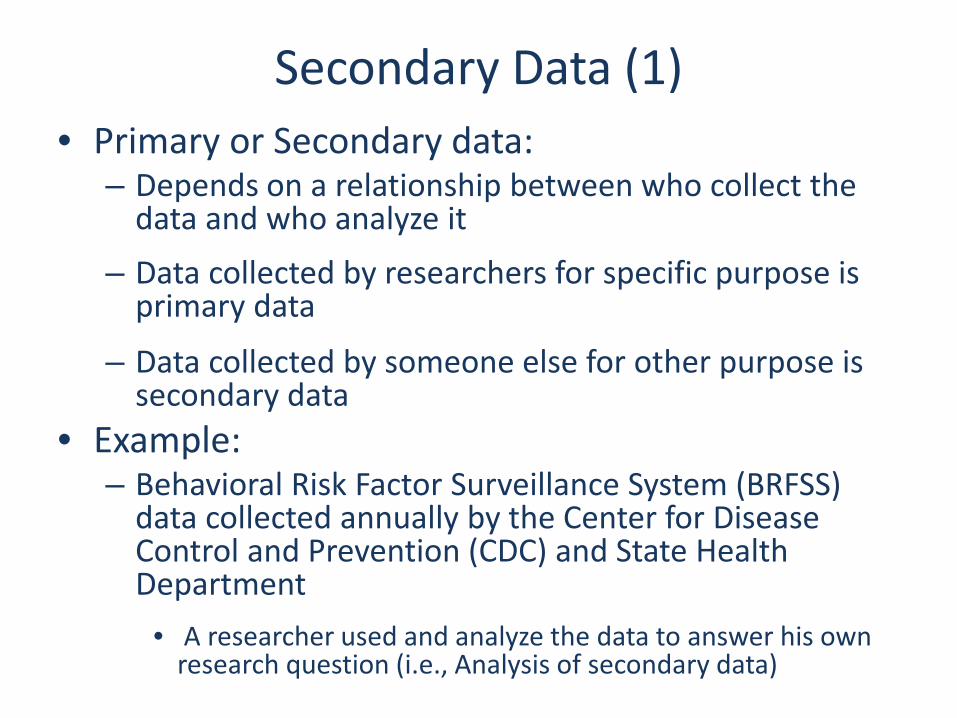
Secondary Data (1)• Primary or Secondary data:

– Depends on a relationship between who collect the data and who analyze it

– Data collected by researchers for specific purpose is primary data

– Data collected by someone else for other purpose is secondary data

• Example:– Behavioral Risk Factor Surveillance System (BRFSS) data collected annually by the Center for Disease Control and Prevention (CDC) and State Health Department 

• A researcher used and analyze the data to answer his own research question (i.e., Analysis of secondary data) 

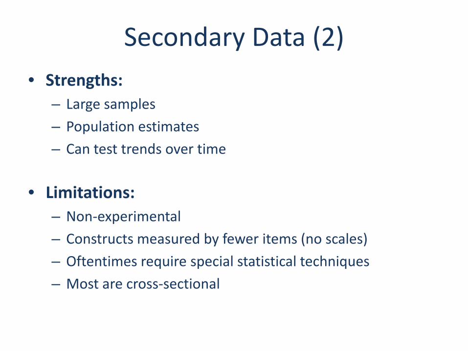
• Strengths:– Large samples

– Population estimates

– Can test trends over time

• Limitations:– Non‐experimental

– Constructs measured by fewer items (no scales)

– Oftentimes require special statistical techniques

– Most are cross‐sectional

Secondary Data (2)

Secondary Data (3)

• Usage:– Pilot data for grant (e.g., R01) proposals

– Hypothesis generation/testing

– Publications

• Types:

– National Health Survey Data

– State Health Survey Data

Behavioral Risk Factor Surveillance System (BRFSS)

http://www.cdc.gov/brfss/

PopulationAdults

MethodRandom Digit Dial telephone surveyState Administration

ContentBehaviors associated with chronic diseases, injuries, and infectious diseases

Sexual behaviorSmokingCancer screeningDiet and exercise

Data>150,000 subjects/yearCore questions asked of everyone and state‐specific modulesData can be combined across states to get national estimates

California Health Interview Survey http://www.chis.ucla.edu

PopulationAdult, adolescent and child questionnairesVery diverse racial/ethnic population

MethodTelephone survey of all California counties

Content Physical activityHealth statusHealth conditionsCancer screeningDietSociodemographic information

Data2001, 2003, 2005, and 2007 data available (2009 underway)~40‐50,000 respondents/survey

NoteMany Latino and Asian groups represented

National Health Interview Survey (NHIS)         

http://www.cdc.gov/nchs/nhis.htm

PopulationHouseholds, families, adults and children

MethodFace to face interview

ContentHealth conditions and behaviors, access to and use of health servicesCancer Control Module (1987, 1992, 2000, 2003, and 2005)

Energy BalanceCancer Screening Sun Avoidance Tobacco Use and Control Genetic Testing

Datan~40,000 households (~87,000 individuals)Initiated in 1957

http://hints.cancer.gov

PopulationAdults (18+)

MethodRandom digit dial (RDD)Conducted Biennially

ContentCommunications trends and practices Cancer information access and usage Cancer risk perceptionMental models of cancerHealth behaviors

Data2003 (n= 6,469); 2005 (n= 5,586)HINTS 2007 data available to public February 16, 2009

Health Information National Trend Survey (HINTS)      

http://www.bls.census.gov/cps/cpsmain.htm

PopulationPart of the Current Population Survey

Method75% telephone 25% in‐home

Content:Cigarette smoking prevalenceCurrent and past cigarette consumption Cigarette smoking quit attempts and intentions to quitCigar, pipe, chewing tobacco, and snuff useDegree of youth access to tobacco in the community Attitudes toward advertising and promotion of tobacco

DataSample of ~240,000 respondents in a given survey periodPart of CPS since 1992

Tobacco Use Supplement – Current Population Survey

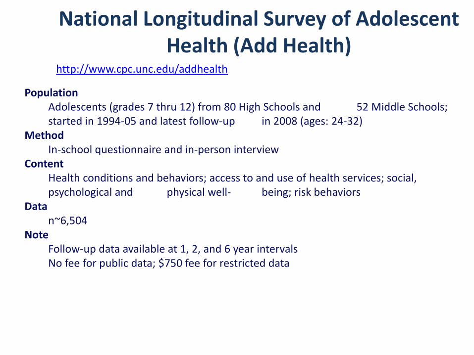
National Longitudinal Survey of Adolescent Health (Add Health)

http://www.cpc.unc.edu/addhealth

PopulationAdolescents (grades 7 thru 12) from 80 High Schools and  52 Middle Schools; started in 1994‐05 and latest follow‐up  in 2008 (ages: 24‐32) 

MethodIn‐school questionnaire and in‐person interview 

ContentHealth conditions and behaviors; access to and use of health services; social, psychological and  physical well‐ being; risk behaviors

Datan~6,504

NoteFollow‐up data available at 1, 2, and 6 year intervalsNo fee for public data; $750 fee for restricted data

Surveillance Epidemiology and End Results (SEER)

http://seer.cancer.gov/

PopulationChildren to adults

MethodData collected from cancer registries that cover ~26% of the US population; follow‐up with individual cases until death

ContentCancer incidence, prevalence, and survival data; limited demographics (age, race/ethnicity, region)

Data100% of cancer cases in registries; Six million cases with 350,000 added each year; 1973 to 2006

NoteNeed specialized software to analyze (SEER*Stat or SEER*Prep)  downloaded from website;Must sign user agreement to obtain; limited to research purposes;

Can be linked to Medicare data

SEER‐Medicare Database

• The linkage of two large population‐based sources of data (Seer + Medicare) 

• can be used for an array of epidemiological and health services research (the use of cancer tests and procedures and the costs of cancer treatment can be examined).

• Are not public use files. Investigators are required to obtain approval in order to acquire data.

National Health and Nutrition Examination Survey 

(NHANES)

http://www.cdc.gov/nchs/nhanes.htm

PopulationChildren and Adults 

MethodFace to face interviewPhysical exams

Content Chronic and Infectious DiseaseMental health and cognitive functioningEnergy BalanceReproductive history and sexual behaviorRespiratory disease

DataN~5000/YearInitiated in 1960’s; Annual since 1999On‐line tutorial

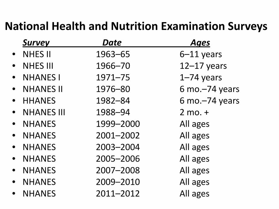
National Health and Nutrition Examination SurveysSurvey Date Ages     

• NHES II  1963–65  6–11 years• NHES III  1966–70  12–17 years• NHANES I  1971–75  1–74 years• NHANES II  1976–80  6 mo.–74 years• HHANES  1982–84  6 mo.–74 years• NHANES III  1988–94  2 mo. +• NHANES  1999–2000  All ages• NHANES  2001–2002  All ages• NHANES  2003–2004  All ages• NHANES  2005–2006  All ages• NHANES  2007–2008  All ages• NHANES  2009–2010  All ages• NHANES  2011–2012  All ages

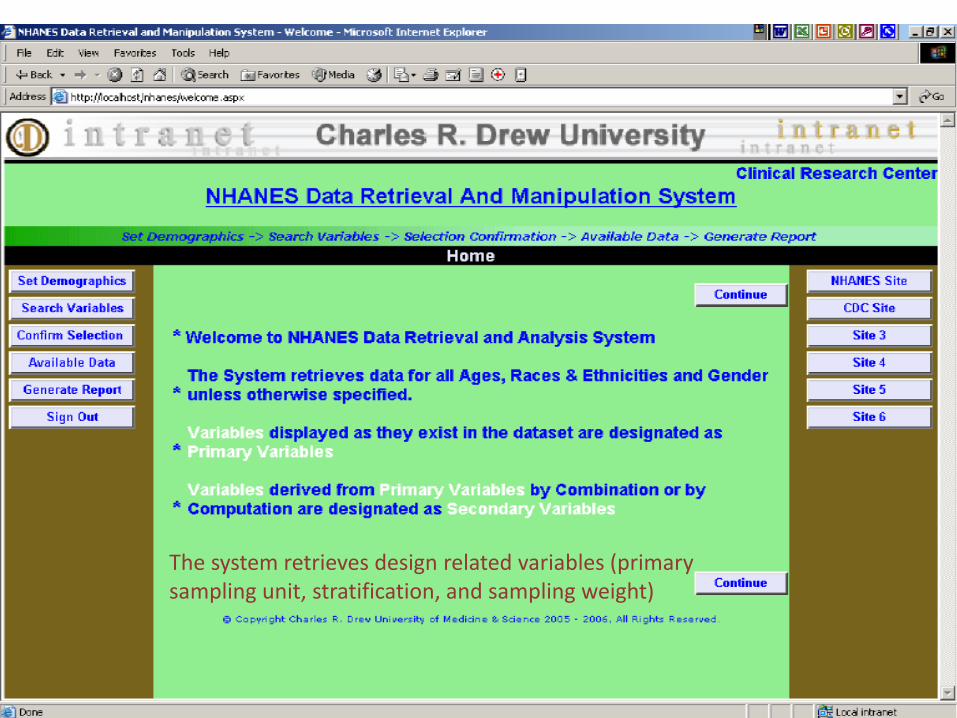
NHANES Data Retrieval & Manipulation System Software Overview (1)

• Product functional capabilities: 

– Give an opportunity to :

• visualize, explore, query and analyze data. 

• display, query, summarize, and organize the NHANES data 

• generate a visual representation of the desired data 

• download the required data in a file format specified by the user.

• The following users will be able to use the system:

1. Faculty of the Charles Drew University of Medicine and Science.

2. Researchers of the Charles Drew University of Medicine and Science.

3. Students of the Charles Drew University of Medicine and Science.

Software Overview (2)• General constraints: 

– Currently only NHANES Data are available for analysis and use. 

– Some training may be required for the users for optimum use of the system.

• The Specification assumes that:

1. No Changes of the historical data takes place in future

2. New data are to be added to the system every year, which must conform to the standard as, laid out in the Database Design Documentation.

3. The Data under consideration is complete and intact.

Attributes• Security: 

– The system is a password‐protected application and each user needs to use his/her credentials to log into the system. 

– There is a default session time for each user session and if left inactive in a logged in state the system will automatically logged off after the session time is over. 

– The user passwords are stored in an encrypted format in the database. – The Administrator is in charge in maintaining the user.

• Reliability, Availability, Maintainance: – The system has an optimum reliability, a high uptime and does not require any 

maintenance.

• Configuration and Compatibility: – The system is not required to be configured for individual customization, because it is 

configured automatically. – The system is not also designed for any other computing environments.

• Installation: – The system is already installed on the Web Server by the developer and does not require 

any special installation. 

• Usability: – The system has a high usability with extremely good user‐friendliness like error messages 

that direct the user to a solution, input range checking as soon as entries are made, and order of choices and screens corresponding to user preferences.

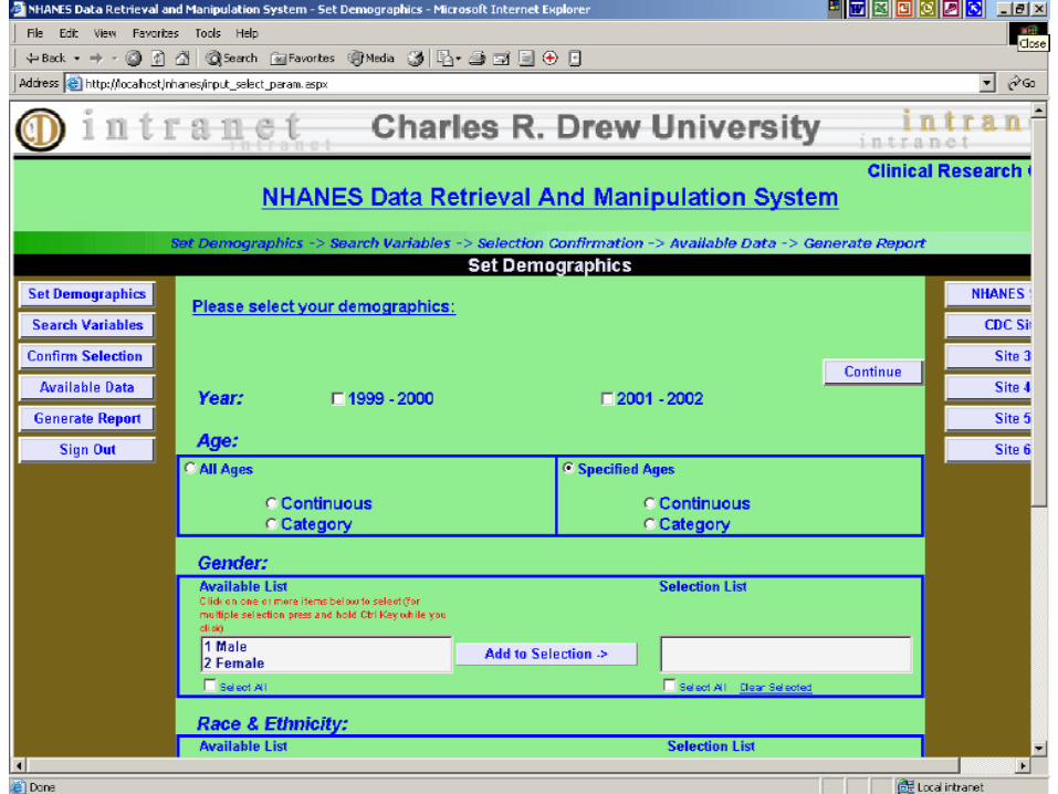
Software Interface (1)

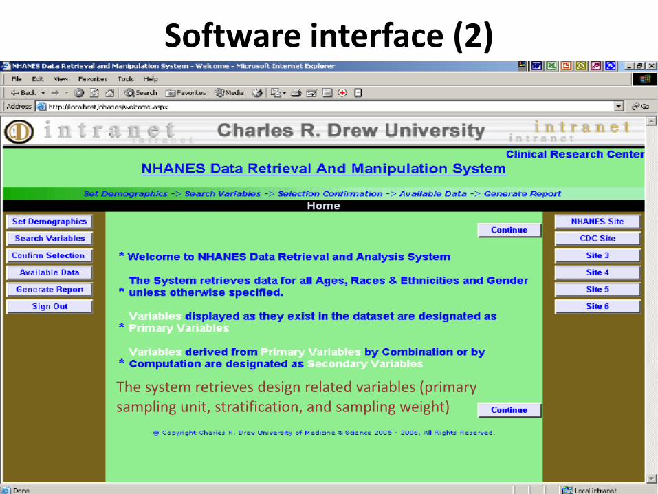
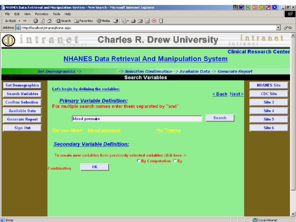
Software interface (2)

The system retrieves design related variables (primary sampling unit, stratification, and sampling weight) 

Other SurveysNational Longitudinal Mortality Study

http://www.census.gov/nlms/National Health Care Survey

http://www.cdc.gov/nchs/nhcs.htmNational Ambulatory Medical Care Survey

http://www.cdc.gov/nchs/about/major/ahcd/ahcd1.htmMedical Expenditure Panel Survey

http://www.meps.ahrq.gov/Medicare Current Beneficiary Survey

http://www.cms.hhs.gov/MCBS/Medicare Health Outcomes Survey

http://www.hosonline.org/National Survey on Drug Use and Health

http://www.oas.samhsa.gov/nhsda.htmNational Survey of Family Growth

http://www.cdc.gov/nchs/about/major/nsfg/nsfgbiblio.htmAmerican Time Use Survey http://www.bls.gov/tus/

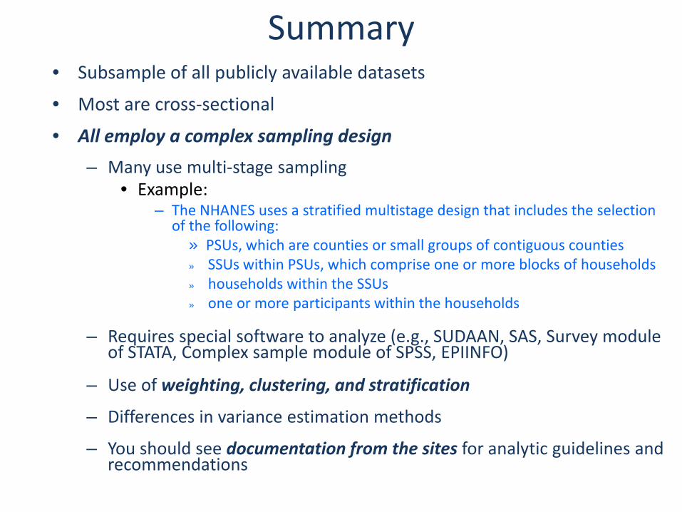
Summary• Subsample of all publicly available datasets

• Most are cross‐sectional

• All employ a complex sampling design

– Many use multi‐stage sampling• Example: 

– The NHANES uses a stratified multistage design that includes the selection of the following:

» PSUs, which are counties or small groups of contiguous counties» SSUs within PSUs, which comprise one or more blocks of households» households within the SSUs» one or more participants within the households

– Requires special software to analyze (e.g., SUDAAN, SAS, Survey module of STATA, Complex sample module of SPSS, EPIINFO)

– Use of weighting, clustering, and stratification

– Differences in variance estimation methods

– You should see documentation from the sites for analytic guidelines and recommendations 

Complex Survey Designs

• Stratification

• Clustering

• Unequal Probabilities of Selection

Traditional calculations give incorrect point estimates; easily fixed through weighting

Traditional statistical calculations give incorrect variance estimates

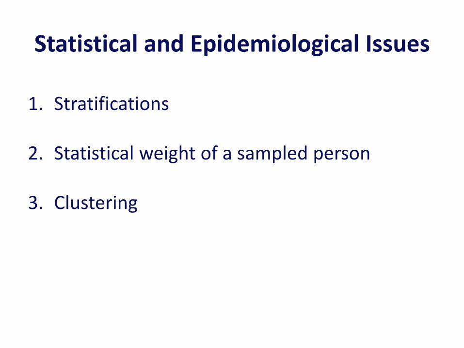
Statistical and Epidemiological Issues

1. Stratifications

2. Statistical weight of a sampled person

3. Clustering

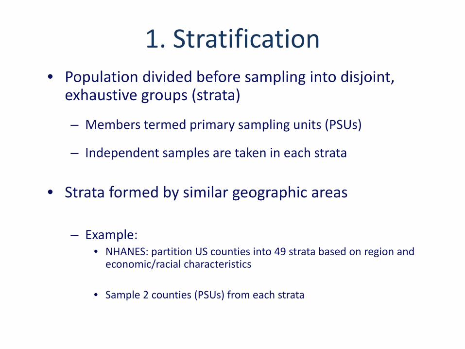
1. Stratification• Population divided before sampling into disjoint, 

exhaustive groups (strata)

– Members termed primary sampling units (PSUs) 

– Independent samples are taken in each strata

• Strata formed by similar geographic areas 

– Example:• NHANES: partition US counties into 49 strata based on region and economic/racial characteristics

• Sample 2 counties (PSUs) from each strata

Simple Random Sample (Random sample of list)

1 324 5 6 7 8 9 10 11

12131415161718192021

2223

24 2526

2728

29 30 3132

3334353637383940

41 42 43 44 45 46 47 48 49 50 51

52

53545556

57585960

2 6

18

26

3740

44 49

5359

Separate population into two or more strata and count number in each

1 324 5 6

78 9 10 11

1213

1415

87654321

1716

1514

1312 11 10

9

2225242321201918

36 35 3433 32 31

3029 28 27 26

45

44434241

4039

3837

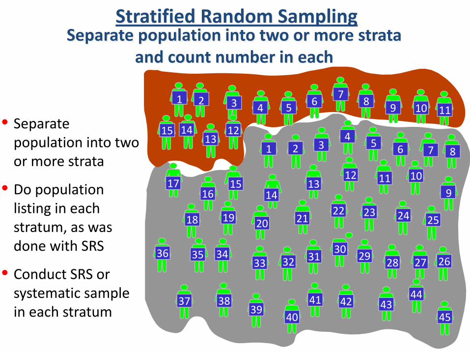
Stratified Random Sampling

• Separate population into two or more strata

• Do population listing in each stratum, as was done with SRS

• Conduct SRS or systematic sample in each stratum

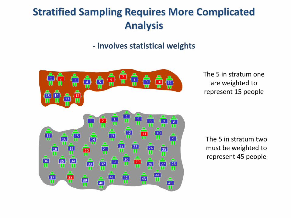
Stratified Sampling Requires More Complicated Analysis

‐ involves statistical weights

87654

321

1716

1514

1312 11

36 35 3433 32 31

3029

28 27

10

9

2524232221201918

26

45

44434241

4039

3837

The 5 in stratum two must be weighted to represent 45 people

1 324 5

67

89 10 11

1213

1415

The 5 in stratum one are weighted to 

represent 15 people

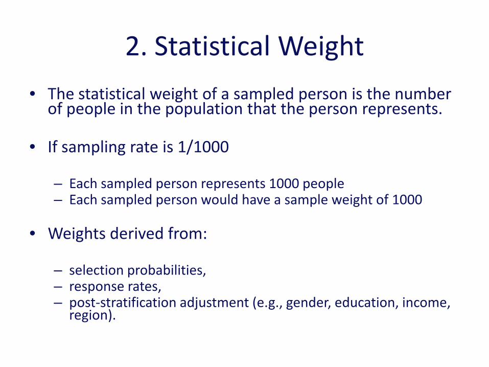
2. Statistical Weight

• The statistical weight of a sampled person is the number of people in the population that the person represents. 

• If sampling rate is 1/1000 

– Each sampled person represents 1000 people – Each sampled person would have a sample weight of 1000

• Weights derived from:

– selection probabilities, – response rates, – post‐stratification adjustment (e.g., gender, education, income, 

region).

HINTS (2003): Older People Participated at a Higher Rate Female participated at higher rate

Unweighted Analysis would have:

Participation increased with educationMinorities were oversampled

* Too many African Americans and Hispanics* Too many 45+ and too few 18-34 year olds* Too many females and too few males* Too many people with high education

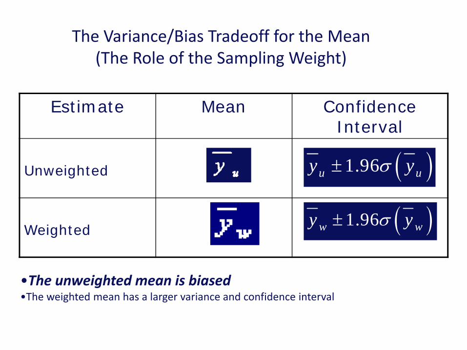
The Variance/Bias Tradeoff for the Mean(The Role of the Sampling Weight)

Estimate Mean Confidence Interval

Unweighted

Weighted

•The unweighted mean is biased•The weighted mean has a larger variance and confidence interval

( )1.96u uy yσ±

( )1.96w wy yσ±

Example: Glycohemoglobin Level (Ghb)• A blood test that measures the amount of glucose bound to hemoglobin.

• Normally, about 4% to 6%.• The test indicates how well diabetes has been controlled in the 2 to 3 months before the test.

• Suppose that we would like to assess the distribution of glycohemoglobin levels. 

• Sampling weights must be considered before plotting a histogram.

SAS Code: Account for Weightsproc univariate data=explore.glyco noprint;

var glyco;

freq weight;

histogram / nrows=2 cfill=red midpoints=3 to 15 by 0.5 cgrid=grayDD;

run;• The variable weight indicates the number of population units the sample 

unit represents.

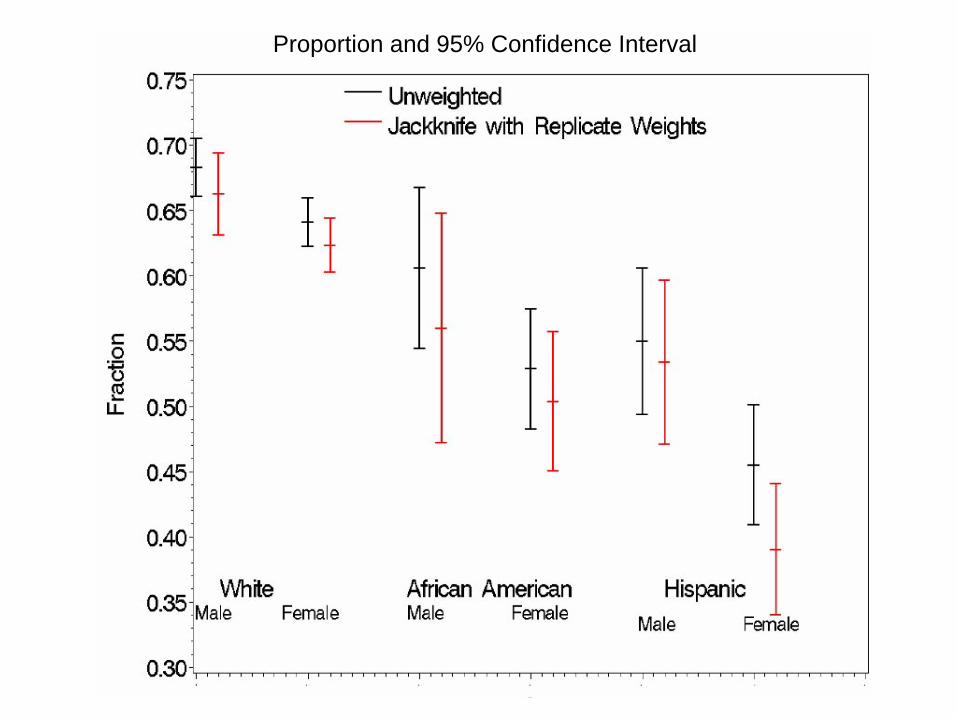
Proportion and 95% Confidence Interval

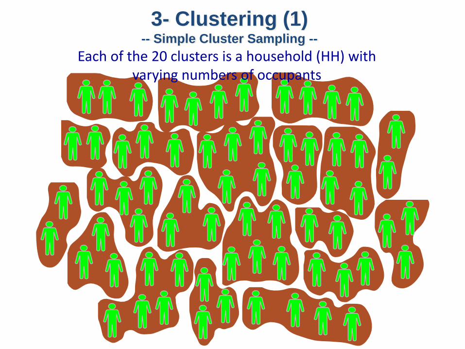
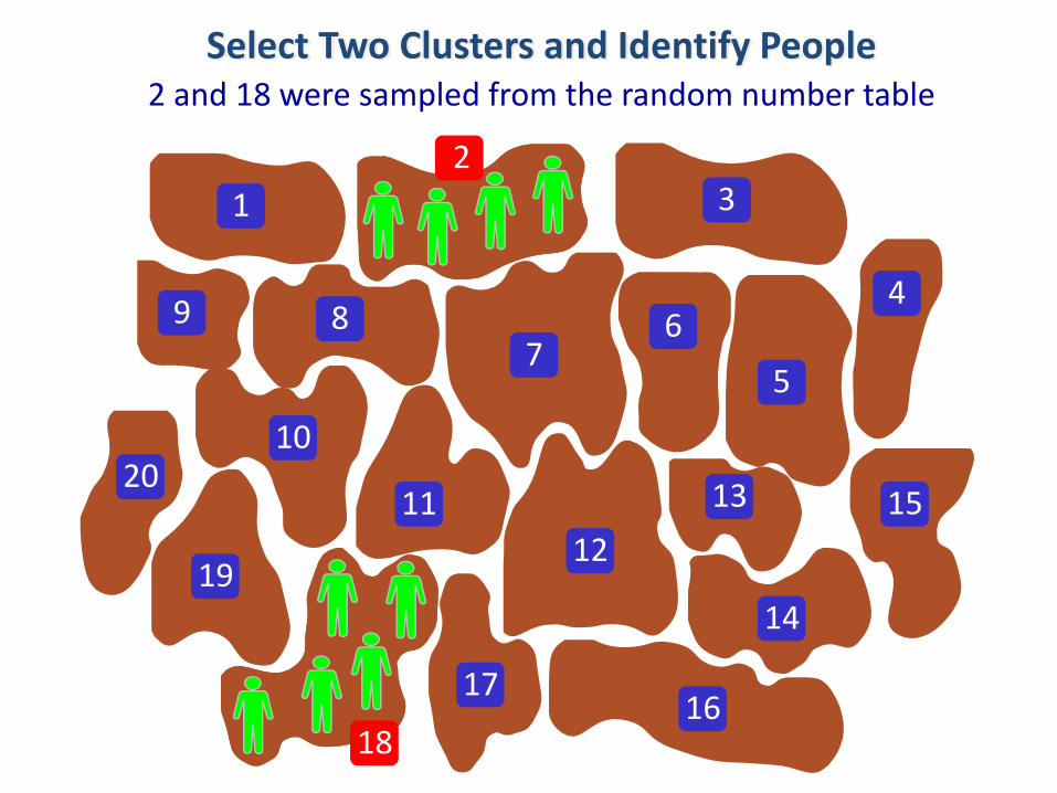
3- Clustering (1)-- Simple Cluster Sampling --

Each of the 20 clusters is a household (HH) with varying numbers of occupants

1 2 3

4

5

67

89

10

1112

13

14

15

1617

18

19

20

Select Two Clusters and Identify People

2

18

2 and 18 were sampled from the random number table

3. Clustering (2)• Persons residing in a small area may have similar 

characteristics

• Thus, responses of subjects in small area (or within an exchange) may be correlated 

• Dependence between subjects leads to inflated variance

• Correlation must be accounted for in the analysis 

– Survey analysis programs do this through strata/PSU

• Area samples may have more clustering than telephone samples

Variance Estimation for Surveys

• Linearization: Uses a Taylor series expansion to estimate variance of non‐linear estimators 

– Default method for most stats programs

– Requires stratification and PSU information

• Replication methods: Calculates different parameter estimates for each replicate and combines these to estimate variance. 

– Jackknife with replicate weights available for a number of SUDAAN, STATA, SAS and WesVAR procedures

Statistical Software for Analyzing Health Surveys

– SAS version 9 ..– STATA ‐‐ Survey module– SPSS – Complex Samples module– EPIINFO for windows – Complex Sample Analysis

Selection of Softweare to Use for Analysis

For correct variance estimates need program that can incorporate complex sampling design

*Needed when doing statistical testing*Standard errors will tend to be larger*Less likely to make Type I error

HANDS ON SESSION

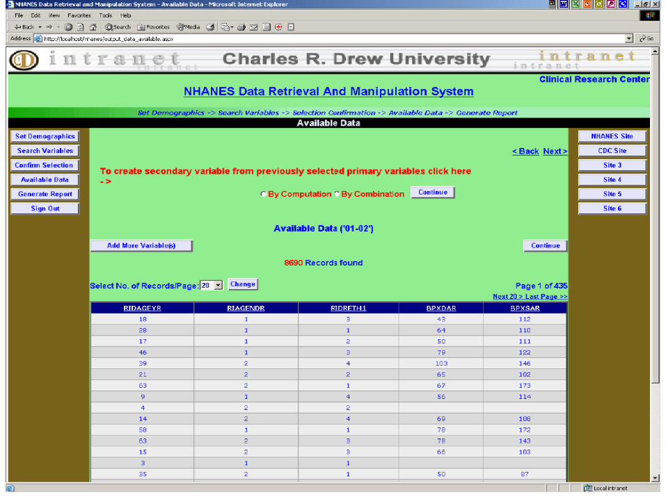
NHANES Data Retrieval & Manipulation System 

The system retrieves design related variables (primary sampling unit, stratification, and sampling weight) 

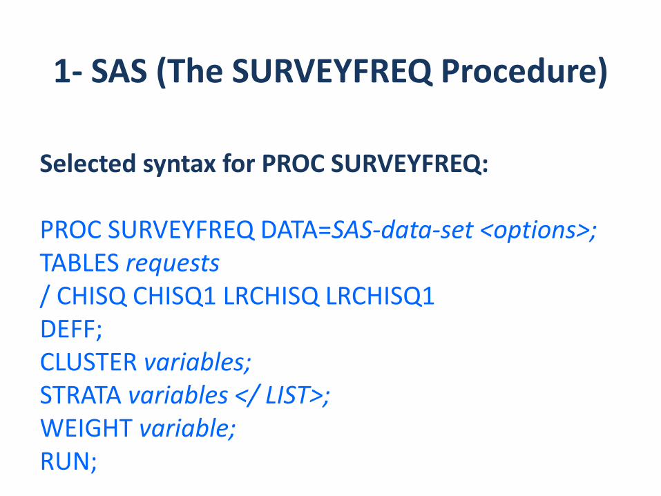
1‐ SAS (The SURVEYFREQ Procedure)

Selected syntax for PROC SURVEYFREQ:

PROC SURVEYFREQ DATA=SAS‐data‐set <options>;TABLES requests/ CHISQ CHISQ1 LRCHISQ LRCHISQ1DEFF;CLUSTER variables;STRATA variables </ LIST>;WEIGHT variable;RUN;

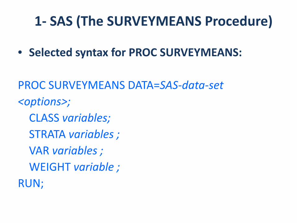
• Selected syntax for PROC SURVEYMEANS:

PROC SURVEYMEANS DATA=SAS‐data‐set<options>;CLASS variables;STRATA variables ;VAR variables ;WEIGHT variable ;

RUN;

1‐ SAS (The SURVEYMEANS Procedure)

1‐ SAS (The SURVEYREG Procedure)Selected statements of the SURVEYREG procedure:

The SURVEYREG Procedure

PROC SURVEYREG <options>;CLASS variables;STRATA variables ;MODEL dependent=<effects> </options> ;WEIGHT variable ;ESTIMATE ‘label’ effect values<effect values …>

RUN;

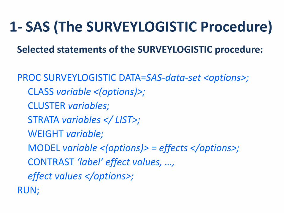
1‐ SAS (The SURVEYLOGISTIC Procedure)Selected statements of the SURVEYLOGISTIC procedure:

PROC SURVEYLOGISTIC DATA=SAS‐data‐set <options>;CLASS variable <(options)>;CLUSTER variables;STRATA variables </ LIST>;WEIGHT variable;MODEL variable <(options)> = effects </options>;CONTRAST ‘label’ effect values, …,effect values </options>;

RUN;

2‐ STATA (EXAMPLE 1)Set memory 4m   

– If you are using Intercooled STATA

use "H:\secondary data workshop\dental2_st_9.dta"

svyset [pweight=wtpfex6], strata(sdpstra6) psu(sdppsu6) 

svy: tabulate needcaresvy: tabulate dentalcariessvy: tabulate hssex dentalcaries, row cisvy: tabulate  hssex needcare, row cisvy: logistic dentalcaries hssexsvy: logistic needcare hssex

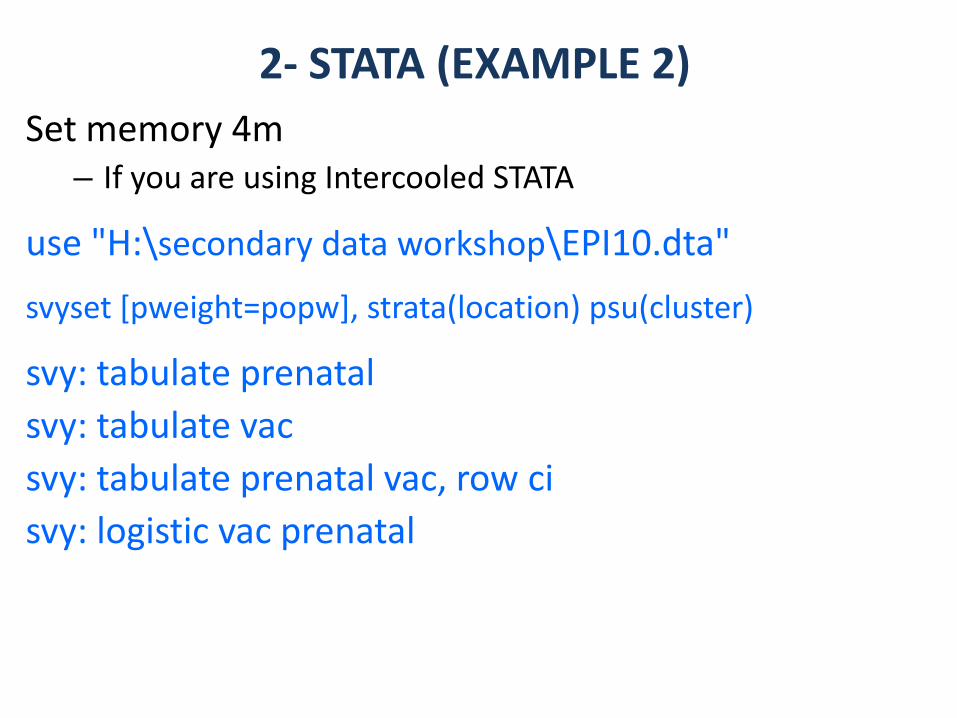
2‐ STATA (EXAMPLE 2)Set memory 4m   

– If you are using Intercooled STATA

use "H:\secondary data workshop\EPI10.dta"

svyset [pweight=popw], strata(location) psu(cluster) 

svy: tabulate prenatalsvy: tabulate vacsvy: tabulate prenatal vac, row cisvy: logistic vac prenatal

3‐ SPSS (Sample Plan)

• Sampling Plan: – Enables you to specify the sampling frame to create a complex sample design used by companion procedures in the SPSS Complex Samples module

– EXAMPLE– CSPLAN ANALYSIS

– /PLAN FILE='F:\secondary data workshop\EPI10_SPSS.csaplan'

– /PLANVARS ANALYSISWEIGHT=POPW       

– /SRSESTIMATOR TYPE=WOR

– /PRINT PLAN

– /DESIGN STRATA=LOCATION CLUSTER=CLUSTER 

– /ESTIMATOR TYPE=WR.

3‐ SPSS (Syntax)

* Complex Samples Frequencies.

CSTABULATE

/PLAN FILE='F:\secondary data workshop\EPI10_SPSS.csaplan'

/TABLES VARIABLES=PRENATAL VAC

/CELLS POPSIZE TABLEPCT

/STATISTICS SE CIN(95) COUNT DEFF 

/MISSING SCOPE=TABLE CLASSMISSING=EXCLUDE.

* Complex Samples Crosstabs.

CSTABULATE

/PLAN FILE='F:\secondary data workshop\EPI10_SPSS.csaplan'

/TABLES VARIABLES=PRENATAL BY VAC

/CELLS POPSIZE ROWPCT COLPCT

/STATISTICS SE CIN(95) COUNT DEFF

/TEST ODDSRATIO INDEPENDENCE

/MISSING SCOPE=TABLE CLASSMISSING=EXCLUDE.

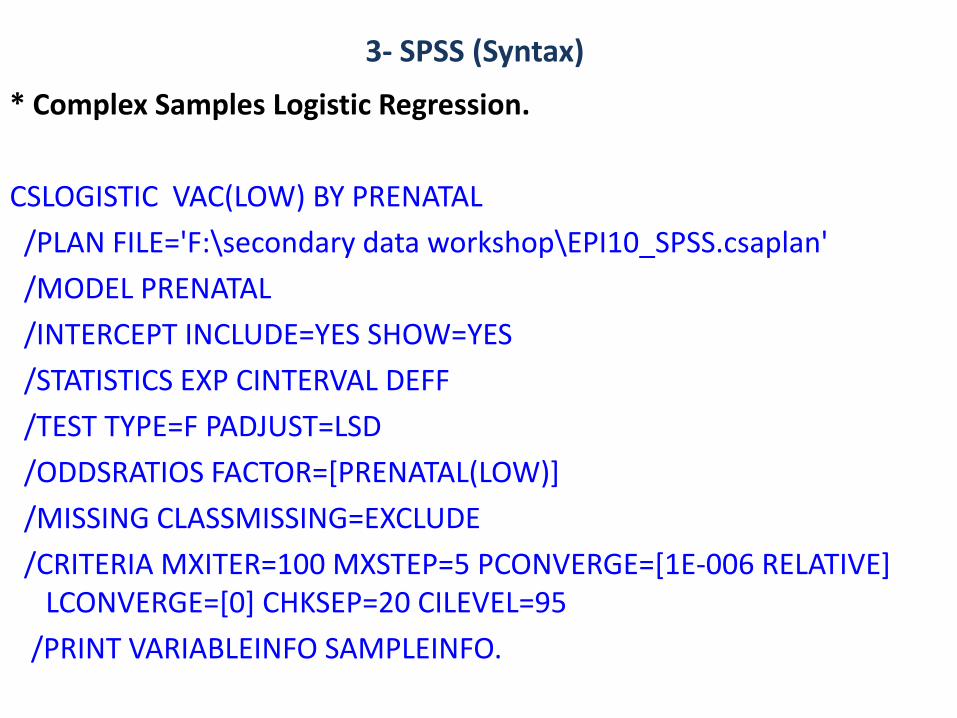
3‐ SPSS (Syntax)

* Complex Samples Logistic Regression.

CSLOGISTIC  VAC(LOW) BY PRENATAL

/PLAN FILE='F:\secondary data workshop\EPI10_SPSS.csaplan' 

/MODEL PRENATAL

/INTERCEPT INCLUDE=YES SHOW=YES

/STATISTICS EXP CINTERVAL DEFF

/TEST TYPE=F PADJUST=LSD

/ODDSRATIOS FACTOR=[PRENATAL(LOW)]

/MISSING CLASSMISSING=EXCLUDE

/CRITERIA MXITER=100 MXSTEP=5 PCONVERGE=[1E‐006 RELATIVE] LCONVERGE=[0] CHKSEP=20 CILEVEL=95

/PRINT VARIABLEINFO SAMPLEINFO.

4‐ EPIINFO 

• Complex Sample Descriptives

• Complex Sample Tabulate

Data/Research Resources• Univ. of Michigan Consortium for social research: 

http://www.icpsr.umich.edu/

• UCLA Statistical Computing: http://www.ats.ucla.edu/stat/

• BRFSS Maps    http://apps.nccd.cdc.gov/gisbrfss/default.aspx

• State Cancer Profiles   http://statecancerprofiles.cancer.gov/

• http://www.cdc.gov/nchs/express.htm

• http://www.ahrq.gov/

• http://www.census.gov/

• http://www.oshpd.ca.gov/SITEMAP.htm

• http://seer.cancer.gov/data/

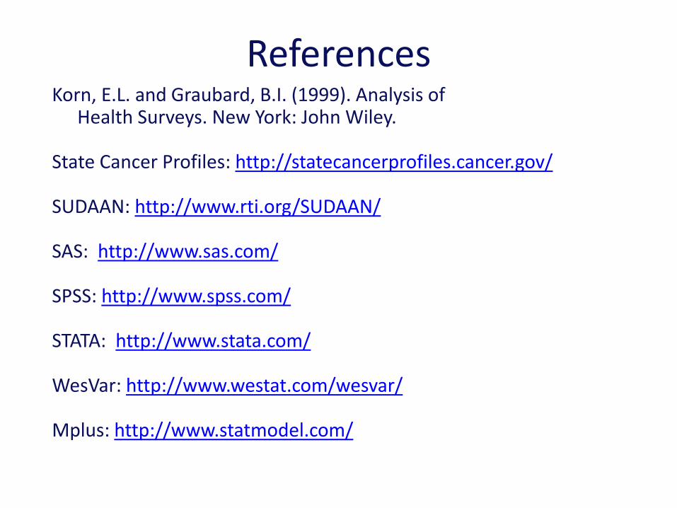
ReferencesKorn, E.L. and Graubard, B.I. (1999). Analysis of 

Health Surveys. New York: John Wiley.

State Cancer Profiles: http://statecancerprofiles.cancer.gov/

SUDAAN: http://www.rti.org/SUDAAN/

SAS:  http://www.sas.com/

SPSS: http://www.spss.com/

STATA:  http://www.stata.com/

WesVar: http://www.westat.com/wesvar/

Mplus: http://www.statmodel.com/

THANK YOU

FEEDBACK AND EVALUATION