Embed Size (px)
Citation preview
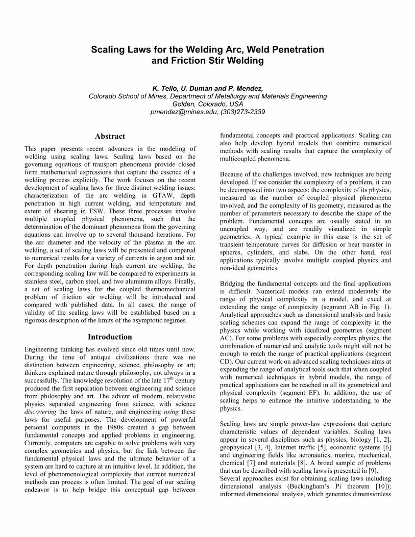
Scaling Laws for the Welding Arc, Weld Penetration and Friction Stir Welding
K. Tello, U. Duman and P. Mendez, Colorado School of Mines, Department of Metallurgy and Materials Engineering
Golden, Colorado, USA [email protected], (303)273-2339
Abstract This paper presents recent advances in the modeling of welding using scaling laws. Scaling laws based on the governing equations of transport phenomena provide closed form mathematical expressions that capture the essence of a welding process explicitly. The work focuses on the recent development of scaling laws for three distinct welding issues: characterization of the arc welding in GTAW, depth penetration in high current welding, and temperature and extent of shearing in FSW. These three processes involve multiple coupled physical phenomena, such that the determination of the dominant phenomena from the governing equations can involve up to several thousand iterations. For the arc diameter and the velocity of the plasma in the arc welding, a set of scaling laws will be presented and compared to numerical results for a variety of currents in argon and air. For depth penetration during high current arc welding, the corresponding scaling law will be compared to experiments in stainless steel, carbon steel, and two aluminum alloys. Finally, a set of scaling laws for the coupled thermomechanical problem of friction stir welding will be introduced and compared with published data. In all cases, the range of validity of the scaling laws will be established based on a rigorous description of the limits of the asymptotic regimes.
Introduction Engineering thinking has evolved since old times until now. During the time of antique civilizations there was no distinction between engineering, science, philosophy or art; thinkers explained nature through philosophy, not always in a successfully. The knowledge revolution of the late 17th century produced the first separation between engineering and science from philosophy and art. The advent of modern, relativistic physics separated engineering from science, with science discovering the laws of nature, and engineering using these laws for useful purposes. The development of powerful personal computers in the 1980s created a gap between fundamental concepts and applied problems in engineering. Currently, computers are capable to solve problems with very complex geometries and physics, but the link between the fundamental physical laws and the ultimate behavior of a system are hard to capture at an intuitive level. In addition, the level of phenomenological complexity that current numerical methods can process is often limited. The goal of our scaling endeavor is to help bridge this conceptual gap between
fundamental concepts and practical applications. Scaling can also help develop hybrid models that combine numerical methods with scaling results that capture the complexity of multicoupled phenomena. Because of the challenges involved, new techniques are being developed. If we consider the complexity of a problem, it can be decomposed into two aspects: the complexity of its physics, measured as the number of coupled physical phenomena involved, and the complexity of its geometry, measured as the number of parameters necessary to describe the shape of the problem. Fundamental concepts are usually stated in an uncoupled way, and are readily visualized in simple geometries. A typical example in this case is the set of transient temperature curves for diffusion or heat transfer in spheres, cylinders, and slabs. On the other hand, real applications typically involve multiple coupled physics and non-ideal geometries. Bridging the fundamental concepts and the final applications is difficult. Numerical models can extend moderately the range of physical complexity in a model, and excel at extending the range of complexity (segment AB in Fig. 1). Analytical approaches such as dimensional analysis and basic scaling schemes can expand the range of complexity in the physics while working with idealized geometries (segment AC). For some problems with especially complex physics, the combination of numerical and analytic tools might still not be enough to reach the range of practical applications (segment CD). Our current work on advanced scaling techniques aims at expanding the range of analytical tools such that when coupled with numerical techniques in hybrid models, the range of practical applications can be reached in all its geometrical and physical complexity (segment EF). In addition, the use of scaling helps to enhance the intuitive understanding to the physics. Scaling laws are simple power-law expressions that capture characteristic values of dependent variables. Scaling laws appear in several disciplines such as physics, biology [1, 2], geophysical [3, 4], Internet traffic [5], economic systems [6] and engineering fields like aeronautics, marine, mechanical, chemical [7] and materials [8]. A broad sample of problems that can be described with scaling laws is presented in [9]. Several approaches exist for obtaining scaling laws including dimensional analysis (Buckingham’s Pi theorem [10]); informed dimensional analysis, which generates dimensionless
groups based on the knowledge about the system [11-16]; inspectional analysis, which generates dimensionless groups from normalized equations; scaling law algorithms (SLAW), which generate scaling laws from statistical data based on a minimum error [17, 18]; and Order of Magnitude Scaling (OMS), in which scaling laws are obtained from equations based on an iterative search for self consistency in identifying the dominant physics [19].
com
plex
ity o
f geo
met
ry(n
umbe
r of p
oint
s to
defin
e it)
num
eric
al
B
Complexity of physics(number of coupled physical phenomena)
Afundamentals
Canalytical
Eadvances scaling(multicoupled, multiphysics)
DF
applications
Fig. 1: Complexity of physics and geonetry can be used to
distinguish fundamental concepts from real-life applications. This construction also helps describe the typical range of
effectiveness of modeling tools.
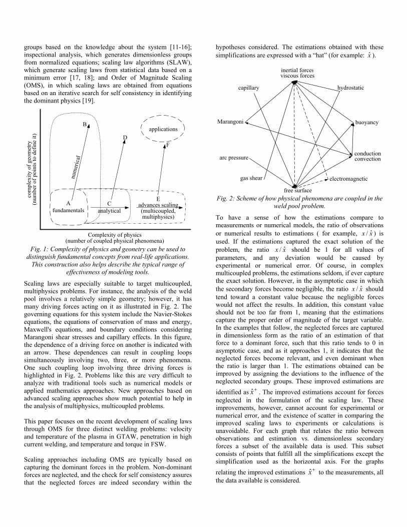
Scaling laws are especially suitable to target multicoupled, multiphysics problems. For instance, the analysis of the weld pool involves a relatively simple geometry; however, it has many driving forces acting on it as illustrated in Fig. 2. The governing equations for this system include the Navier-Stokes equations, the equations of conservation of mass and energy, Maxwell's equations, and boundary conditions considering Marangoni shear stresses and capillary effects. In this figure, the dependence of a driving force on another is indicated with an arrow. These dependences can result in coupling loops simultaneously involving two, three, or more phenomena. One such coupling loop involving three driving forces is highlighted in Fig. 2. Problems like this are very difficult to analyze with traditional tools such as numerical models or applied mathematics approaches. New approaches based on advanced scaling approaches show much potential to help in the analysis of multiphysics, multicoupled problems. This paper focuses on the recent development of scaling laws through OMS for three distinct welding problems: velocity and temperature of the plasma in GTAW, penetration in high current welding, and temperature and torque in FSW. Scaling approaches including OMS are typically based on capturing the dominant forces in the problem. Non-dominant forces are neglected, and the check for self consistency assures that the neglected forces are indeed secondary within the
hypotheses considered. The estimations obtained with these simplifications are expressed with a “hat” (for example: x̂ ).
inertial forcesviscous forces
hydrostatic
buoyancy
conductionconvection
electromagnetic
free surface
gas shear
arc pressure
Marangoni
capillary
Fig. 2: Scheme of how physical phenomena are coupled in the
weld pool problem.
To have a sense of how the estimations compare to measurements or numerical models, the ratio of observations or numerical results to estimations ( for example, xx ˆ/ ) is used. If the estimations captured the exact solution of the problem, the ratio xx ˆ/ should be 1 for all values of parameters, and any deviation would be caused by experimental or numerical error. Of course, in complex multicoupled problems, the estimations seldom, if ever capture the exact solution. However, in the asymptotic case in which the secondary forces become negligible, the ratio xx ˆ/ should tend toward a constant value because the negligible forces would not affect the results. In addition, this constant value should not be too far from 1, meaning that the estimations capture the proper order of magnitude of the target variable. In the examples that follow, the neglected forces are captured in dimensionless form as the ratio of an estimation of that force to a dominant force, such that this ratio tends to 0 in asymptotic case, and as it approaches 1, it indicates that the neglected forces become relevant, and even dominant when the ratio is larger than 1. The estimations obtained can be improved by assigning the deviations to the influence of the neglected secondary groups. These improved estimations are identified as +x̂ . The improved estimations account for forces neglected in the formulation of the scaling law. These improvements, however, cannot account for experimental or numerical error, and the existence of scatter in comparing the improved scaling laws to experiments or calculations is unavoidable. For each graph that relates the ratio between observations and estimation vs. dimensionless secondary forces a subset of the available data is used. This subset consists of points that fulfill all the simplifications except the simplification used as the horizontal axis. For the graphs relating the improved estimations +x̂ to the measurements, all the data available is considered.
Examples
Welding Arc The electric arc is a relevant problem for industrial applications such as welding, steelmaking, and plasma spraying. The scaling analysis in focused on the fluid motion of the plasma in the cathode region of the arc, shadowed region presented in Fig. 1 of [20]. This can be considered essentially isothermal due to its small size compared to the rest of the arc [20]. The driving forces acting on this system are electromagnetic forces in the radial and axial direction, which are opposed by inertial and viscous forces; convection, conduction and radial joule exist in the core of the arc; while, convection, axial conduction and radiation exist in the sheath. For the scaling analysis of the temperature, it is assumed that convection is not important in the column. Fig. 3 of [21] presents a schematic of the temperature profile developed in the welding arc. The governing equations for this system include the conservation of mass, conservation of momentum, Ampere’s law and the conservation of magnetic field expressed in R and Z coordinates. Scaling of these equations has been done in [20], resulting in the following scaling law for axial velocity:
21
21
021ˆ
ρμ CC
ZSJRV = (1)
The fluid mechanics in the cathode region was assumed isothermal, and the ratios of neglected forces to dominant forces are captured by Equations (2) and (3).
1Re1
<< (2)
22RRR
hR cac
Δ<<
(3)
The ionization radius that delimits the core of the arc was scaled in [21], yielding the following scaling law:
( ) 1.00
1.01.04.0
2.02.02.0 2ˆ −−−−− −⎟⎠⎞
⎜⎝⎛= TTSkISkR iRggRTTTi π
σ (4)
where the ratios of the neglected forces are given by Equations (5) through (7).
( ) 1 ...
...2radiation
conduction
4.04.0
4.06.0
7.03.02.0
<<−
⎟⎠⎞
⎜⎝⎛=
−−
oiRg
gRTTT
TTS
kISkπ
σ (5)
( ) 12 ...
...2
5radiation
driftelectron
3.03.03.02.1
4.06.06.0
<<−⎟⎠⎞
⎜⎝⎛
⎟⎠⎞
⎜⎝⎛ Δ
⎟⎟⎠
⎞⎜⎜⎝
⎛=
−
−−
oiRgg
bRTTT
TTSkI
hRI
ek
Sk
π
πσ
(6)
12radiation
radial Joule 22
<<⎟⎠⎞
⎜⎝⎛
⎟⎠⎞
⎜⎝⎛ Δ
=−
IhRI
ππ (7)
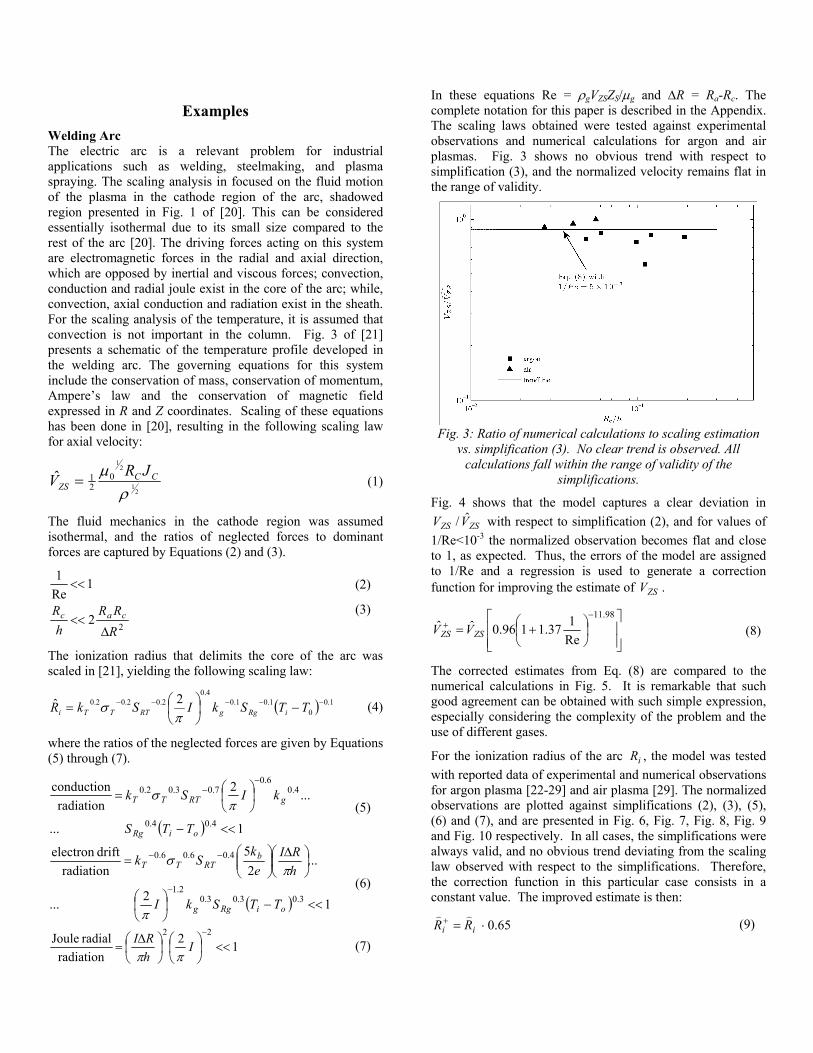
In these equations Re = ρgVZSZS/μg and ΔR = Ra-Rc. The complete notation for this paper is described in the Appendix. The scaling laws obtained were tested against experimental observations and numerical calculations for argon and air plasmas. Fig. 3 shows no obvious trend with respect to simplification (3), and the normalized velocity remains flat in the range of validity.
Fig. 3: Ratio of numerical calculations to scaling estimation
vs. simplification (3). No clear trend is observed. All calculations fall within the range of validity of the
simplifications.
Fig. 4 shows that the model captures a clear deviation in
ZSZS VV ˆ/ with respect to simplification (2), and for values of 1/Re<10-3 the normalized observation becomes flat and close to 1, as expected. Thus, the errors of the model are assigned to 1/Re and a regression is used to generate a correction function for improving the estimate of ZSV .
⎥⎥⎦
⎤
⎢⎢⎣
⎡⎟⎠⎞
⎜⎝⎛ +=
−+
98.11
Re137.1196.0ˆˆ
ZSZS VV (8)
The corrected estimates from Eq. (8) are compared to the numerical calculations in Fig. 5. It is remarkable that such good agreement can be obtained with such simple expression, especially considering the complexity of the problem and the use of different gases.
For the ionization radius of the arc iR , the model was tested with reported data of experimental and numerical observations for argon plasma [22-29] and air plasma [29]. The normalized observations are plotted against simplifications (2), (3), (5), (6) and (7), and are presented in Fig. 6, Fig. 7, Fig. 8, Fig. 9 and Fig. 10 respectively. In all cases, the simplifications were always valid, and no obvious trend deviating from the scaling law observed with respect to the simplifications. Therefore, the correction function in this particular case consists in a constant value. The improved estimate is then:
65.0⋅=+ii RR))
(9)
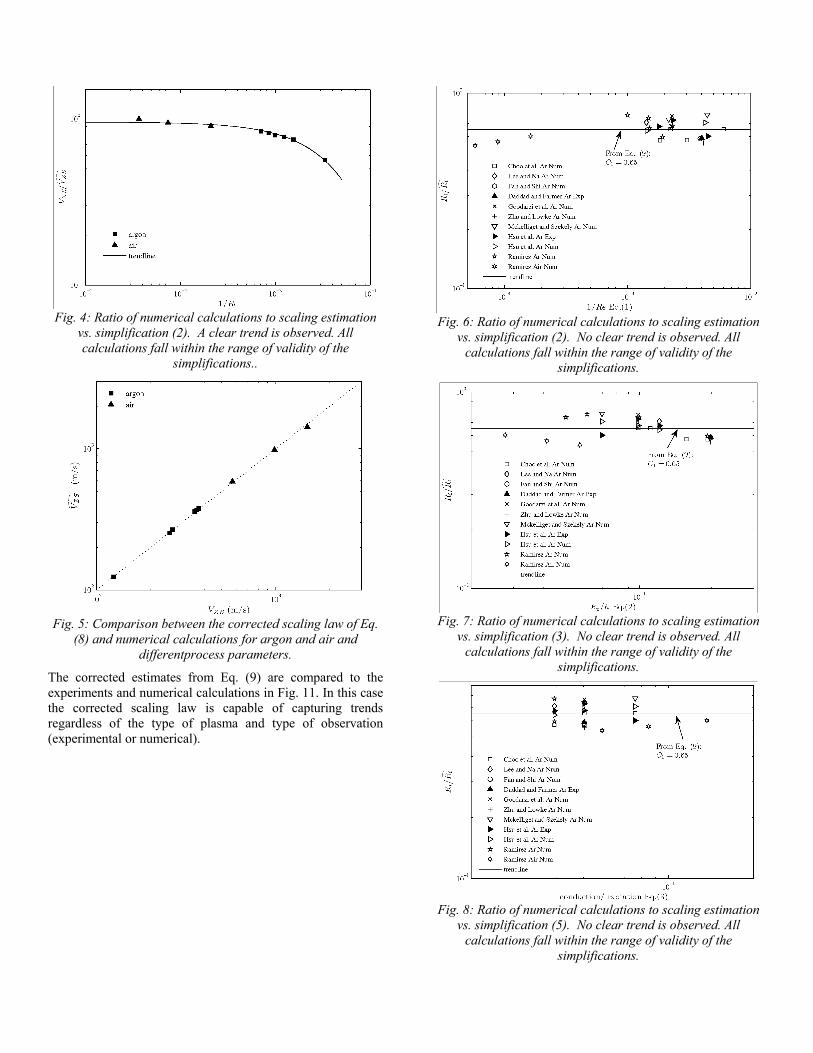
Fig. 4: Ratio of numerical calculations to scaling estimation
vs. simplification (2). A clear trend is observed. All calculations fall within the range of validity of the
simplifications..
Fig. 5: Comparison between the corrected scaling law of Eq.
(8) and numerical calculations for argon and air and differentprocess parameters.
The corrected estimates from Eq. (9) are compared to the experiments and numerical calculations in Fig. 11. In this case the corrected scaling law is capable of capturing trends regardless of the type of plasma and type of observation (experimental or numerical).
Fig. 6: Ratio of numerical calculations to scaling estimation
vs. simplification (2). No clear trend is observed. All calculations fall within the range of validity of the
simplifications.
Fig. 7: Ratio of numerical calculations to scaling estimation
vs. simplification (3). No clear trend is observed. All calculations fall within the range of validity of the
simplifications.
Fig. 8: Ratio of numerical calculations to scaling estimation
vs. simplification (5). No clear trend is observed. All calculations fall within the range of validity of the
simplifications.

Fig. 9: Ratio of numerical calculations to scaling estimation
vs. simplification (6). No clear trend is observed. All calculations fall within the range of validity of the
simplifications.
Fig. 10: Ratio of numerical calculations to scaling estimation
vs. simplification (7). No clear trend is observed. All calculations fall within the range of validity of the
simplifications.
Weld Penetration Weld penetration of high productivity Gas Tungsten Arc Welding (GTAW) involves high current and travel velocity; its analysis is well suited for OMS because it has a relatively simple geometry and multiple coupled driving forces acting on it. Fig. 12 shows a schematic of the weld pool at high current and velocity. It can be seen that the molten metal turns into a thin film under the electrode. The penetration mechanism is the gouging region penetration [22-25], in which no recirculating flows exist. The governing equation is given by Fourier’s law of heat conduction as a function of time and position. Both heat loss by conduction through the sides of the weld and by convection are neglected, and because the high current and speed, the heat transfer becomes a one-dimensional problem in the Z-direction. Quasi-steady state in Lagrangian coordinates is assumed. Three hypotheses commonly valid in practical applications
help simplify the problem. The range of validity of these hypotheses then becomes the limits of validity of the model. The three hypotheses are: 1) The heat source is moving at high speed, 2) the heat from the arc goes directly to melt the material (no heat losses by conduction), and 3) the liquid film over the gouging region is thinner than the penetration depth. These simplifications are captured by Equations (10), (11) and (12) respectively. The notation is described in the Appendix.
Fig. 11: Comparison between the corrected scaling law of
Eq.(9) and experiments or numerical calculations for argon and air and different process parameters
Torch
U
XY
Z
D
Gouging region
Thin liquid film (δ)
σq
L
-∞ ∞
l - coordinate
q(max)
Lw
Torch
U
XY
Z
D
Gouging region
Thin liquid film (δ)
σq
L
-∞ ∞
l - coordinate
q(max)
Lw
Fig. 12: Coordinates and schematic of the thin liquid film at
the gouging region.
11<<=
qUPe σα (10)
121
2max
22<<=
qarc
grad
qUH
σρα (11)
122 maxmax
<<=τμ
σπρδ DU
qUH
D q
(12)
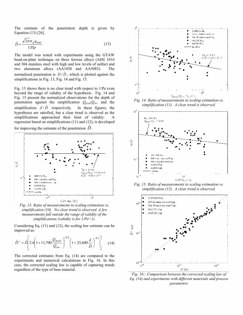
The estimate of the penetration depth is given by Equation (13) [26].
ρσπ
UHq
D q max2ˆ = (13)
The model was tested with experiments using the GTAW bead-on-plate technique on three ferrous alloys (AISI 1016 and 304 stainless steel with high and low levels of sulfur) and two aluminum alloys (AA1020 and AA5083). The normalized penetration is DD ˆ/ , which is plotted against the simplifications in Fig. 13, Fig. 14 and Fig. 15. Fig. 13 shows there is no clear trend with respect to 1/Pe even beyond the range of validity of the hypothesis. Fig. 14 and Fig. 15 present the normalized observations for the depth of penetration against the simplification Qgrad/Qarc and the simplification D̂/δ respectively. In these figures, the hypotheses are satisfied, but a clear trend is observed as the simplifications approached their limit of validity. A regression based on simplifications (11) and (12), is developed for improving the estimate of the penetration D̂ .
Fig. 13: Ratio of measurements to scaling estimation vs.
simplification (10). No clear trend is observed. A few measurements fall outside the range of validity of the
simplifications (validity is for 1/Pe<1).
Considering Eq. (11) and (12), the scaling law estimate can be improved as:
⎥⎥
⎦
⎤
⎢⎢
⎣
⎡⎟⎠
⎞⎜⎝
⎛ +⎟⎟⎠
⎞⎜⎜⎝
⎛+=
−−+
1.02.0
ˆ600,251700,1116.2ˆˆDQ
QDD
arc
grad δ (14)
The corrected estimates from Eq. (14) are compared to the experiments and numerical calculations in Fig. 16. In this case, the corrected scaling law is capable of capturing trends regardless of the type of base material.
Fig. 14: Ratio of measurements to scaling estimation vs.
simplification (11). A clear trend is observed.
Fig. 15: Ratio of measurements to scaling estimation vs.
simplification (12). A clear trend is observed.
Fig. 16:: Comparison between the corrected scaling law of
Eq. (14) and experiments with different materials and process parameters
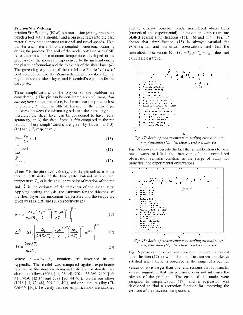
Friction Stir Welding Friction Stir Welding (FSW) is a non-fusion joining process in which a tool with a shoulder and a pin penetrates into the base material moving at constant rotational and travel speeds. Heat transfer and material flow are coupled phenomena occurring during the process. The goal of the model obtained with OMS is to determine the maximum temperature developed in the process (TS), the shear rate experienced by the material during the plastic deformation and the thickness of the shear layer (δ). The governing equations of the model are Fourier’s Law of heat conduction and the Zenner-Hollomon equation for the region inside the shear layer, and Rosenthal’s equation for the base plate. Three simplifications to the physics of the problem are considered: 1) The pin can be considered a steady state, slow moving heat source; therefore, isotherms near the pin are close to circular, 2) there is little difference in the shear layer thickness between the advancing side and the retreating side; therefore, the shear layer can be considered to have radial symmetry, an 3) the shear layer is thin compared to the pin radius. These simplifications are given by Equations (15), (16) and (17) respectively.
12
<<=α
VaPe (15)
1ˆ <<δω
V (16)
1ˆ
<<aδ (17)
where V is the pin travel velocity, a is the pin radius, α is the thermal diffusivity of the base plate material at a critical temperature To, ω is the angular velocity of rotation of the pin and δ̂ is the estimate of the thickness of the shear layer. Applying scaling analysis, the estimates for the thickness of the shear layer, the maximum temperature and the torque are given by (18), (19) and (20) respectively [27].
2/1122ˆ⎥⎥
⎦
⎤
⎢⎢
⎣
⎡
⎟⎟⎠
⎞⎜⎜⎝
⎛Δ⎟
⎟⎠
⎞⎜⎜⎝
⎛Δ=
+n
o
on
R
S
m
TK
ka
ABT
aωητ
ηδ (18)
2/1
1122ˆ
⎥⎥⎦
⎤
⎢⎢⎣
⎡⎟⎟⎠
⎞⎜⎜⎝
⎛Δ⎟⎟
⎠
⎞⎜⎜⎝
⎛Δ
Δ=Δ +
−
nn
o
o
n
R
m
sms T
Kka
TkABTT ωητη (19)
o
o
KTkM
ηωπ Δ
=2ˆ (20)
Where oSS TTT −=Δ , notations are described in the Appendix. The model was compared against experiments reported in literature involving eight different materials: five aluminum alloys (6061 [11, 28-34], 2024 [35-39], 2195 [40, 41], 7050 [42-44] and 5083 [30, 44-46]), two ferrous alloys (1018 [11, 47, 48], 304 [11, 49]), and one titanium alloy (Ti-6Al-4V [50]). To verify that the simplifications are satisfied
and to observe possible trends, normalized observations (numerical and experimental) for maximum temperature are plotted against simplifications (15), (16) and (17). Fig. 17 shows that simplification (15) is always satisfied for experimental and numerical observations and that the normalized observation )ˆ/()( ∞∞ −−=Θ TTTT SS does not exhibit a clear trend.
Fig. 17: Ratio of measurements to scaling estimation vs.
simplification (15). No clear trend is observed.
Fig. 18 shows that despite the fact that simplification (16) was not always satisfied the behavior of the normalized observation remains constant in the range of study for numerical and experimental observations.
Fig. 18: Ratio of measurements to scaling estimation vs.
simplification (16). No clear trend is observed.
Fig. 19 presents the normalized maximum temperature against simplification (17), in which he simplification was no always satisfied and a trend is observed in the range of study for values of a/δ̂ larger than one, and remains flat for smaller values, suggesting that this parameter does not influence the physics of the problem. The errors of the model were assigned to simplification (17), and a regression was developed to find a correction function for improving the estimate of the maximum temperature.
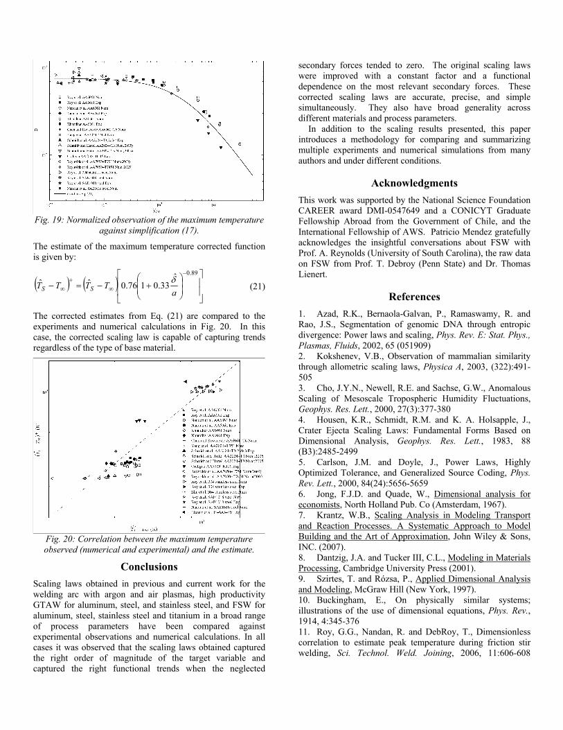
Fig. 19: Normalized observation of the maximum temperature
against simplification (17).
The estimate of the maximum temperature corrected function is given by:
( ) ( )⎥⎥
⎦
⎤
⎢⎢
⎣
⎡
⎟⎟⎠
⎞⎜⎜⎝
⎛+−=−
−
∞+
∞
89.0ˆ33.0176.0ˆˆ
aTTTT SS
δ (21)
The corrected estimates from Eq. (21) are compared to the experiments and numerical calculations in Fig. 20. In this case, the corrected scaling law is capable of capturing trends regardless of the type of base material.
Fig. 20: Correlation between the maximum temperature observed (numerical and experimental) and the estimate.
Conclusions Scaling laws obtained in previous and current work for the welding arc with argon and air plasmas, high productivity GTAW for aluminum, steel, and stainless steel, and FSW for aluminum, steel, stainless steel and titanium in a broad range of process parameters have been compared against experimental observations and numerical calculations. In all cases it was observed that the scaling laws obtained captured the right order of magnitude of the target variable and captured the right functional trends when the neglected
secondary forces tended to zero. The original scaling laws were improved with a constant factor and a functional dependence on the most relevant secondary forces. These corrected scaling laws are accurate, precise, and simple simultaneously. They also have broad generality across different materials and process parameters.
In addition to the scaling results presented, this paper introduces a methodology for comparing and summarizing multiple experiments and numerical simulations from many authors and under different conditions.
Acknowledgments
This work was supported by the National Science Foundation CAREER award DMI-0547649 and a CONICYT Graduate Fellowship Abroad from the Government of Chile, and the International Fellowship of AWS. Patricio Mendez gratefully acknowledges the insightful conversations about FSW with Prof. A. Reynolds (University of South Carolina), the raw data on FSW from Prof. T. Debroy (Penn State) and Dr. Thomas Lienert.
References 1. Azad, R.K., Bernaola-Galvan, P., Ramaswamy, R. and Rao, J.S., Segmentation of genomic DNA through entropic divergence: Power laws and scaling, Phys. Rev. E: Stat. Phys., Plasmas, Fluids, 2002, 65 (051909) 2. Kokshenev, V.B., Observation of mammalian similarity through allometric scaling laws, Physica A, 2003, (322):491-505 3. Cho, J.Y.N., Newell, R.E. and Sachse, G.W., Anomalous Scaling of Mesoscale Tropospheric Humidity Fluctuations, Geophys. Res. Lett., 2000, 27(3):377-380 4. Housen, K.R., Schmidt, R.M. and K. A. Holsapple, J., Crater Ejecta Scaling Laws: Fundamental Forms Based on Dimensional Analysis, Geophys. Res. Lett., 1983, 88 (B3):2485-2499 5. Carlson, J.M. and Doyle, J., Power Laws, Highly Optimized Tolerance, and Generalized Source Coding, Phys. Rev. Lett., 2000, 84(24):5656-5659 6. Jong, F.J.D. and Quade, W., Dimensional analysis for economists, North Holland Pub. Co (Amsterdam, 1967). 7. Krantz, W.B., Scaling Analysis in Modeling Transport and Reaction Processes. A Systematic Approach to Model Building and the Art of Approximation, John Wiley & Sons, INC. (2007). 8. Dantzig, J.A. and Tucker III, C.L., Modeling in Materials Processing, Cambridge University Press (2001). 9. Szirtes, T. and Rózsa, P., Applied Dimensional Analysis and Modeling, McGraw Hill (New York, 1997). 10. Buckingham, E., On physically similar systems; illustrations of the use of dimensional equations, Phys. Rev., 1914, 4:345-376 11. Roy, G.G., Nandan, R. and DebRoy, T., Dimensionless correlation to estimate peak temperature during friction stir welding, Sci. Technol. Weld. Joining, 2006, 11:606-608

12. Murray, P.E., Stability of droplets in gas metal arc welding, Sci. Technol. Weld. Joining, 2000, 5(4):221-226 13. Murray, P.E. and Scotti, A., Depth of penetration in gas metal arc welding, Sci. Technol. Weld. Joining, 1999, 4 (2):112-117 14. Murray, P.E., Selecting Parameters for GMAW Using Dimensional Analysis, Welding Journal, 2002, 81:125S-131S 15. Fuerschbach, P.W. and Knorovsky, G.A., A Study of Melting Efficiency in Plasma Arc and Gas Tungsten Arc Welding, Welding Journal, 1991, 70 (287S-297S) 16. Fuerschbach, P.W. "A dimensionless parameter model for arc welding processes," In 4th international conference on trends in welding research, Gatlinburg, TN (United States), 1995, pp. 493-497. 17. Mendez, P.F. and Ordoñez, F., Scaling Laws from Statistical Data and Dimensional Analysis, J. Appl. Mech., 2005, 72(5):648-657 18. Mendez, P.F., Furrer, R., Ford, R. and Ordóñez, F., Scaling Laws as a Tool of Materials Informatics,, JOM, 2008, 60(3):60-66 19. Mendez, P.F. Advanced scaling thecniques for the modeling of materials processing, In Sohn International Symposium Advanced Processing of Metals and Materials, San Diego, CA, 2006. TMS. 20. Mendez, P.F., Ramirez, M.A., Trapaga, G. and Eagar, T.W., Order-of-Magnitud Scaling of the Cathode Region in an Axisymmetric Transferred Electric Arc, Metall. Mater. Trans. B, 2001, 32B:547-554 21. Mendez, P.F., Ramirez, M.A., Trapaga, G. and Eagar, T.W., Scaling Laws in the Welding Arc, in Mathematical Modelling of Weld Phenomena 6, (2002), H. Cerjak, Editor. pp. 43-61. 22. Mendez, P.F. and Eagar, T.W., Penetration and defect formation in hihg-currrent arc welding, Welding Journal, 2003, 82(10):296S-306S 23. Soderstrom, E. and Mendez, P.F., Humping mechanisms present in high speed welding, Sci. Technol. Weld. Joining, 2006, 11(5):572-579 24. Shimada, W. and Hoshinouchi, S., A Study on Bead Formation of Low Pressure TIG Arc and Prevention on Under-Cut Bead, Quaterly Journal of the Japan Welding Society, 1982, 51(3):280-286 25. Yamamoto, T. and Shimada, W. A Study on Bead Formation in High Speed TIG Arc Welding at Low Gas Pressure, In International Symposium in Welding, Osaka, Japan, 1975. 26. Duman, Ü. and Mendez, P.F. "Weld Penetration at High Velocity GTAW," In Fabtec/AWS Annual Meeting, Chicago, IL, 2007, pp. 107-108. 27. Mendez, P.F. and Lienert, T.J., Non-Adiabatic shearing in Friction Stir Welding, TMS Letter, 2006, 3(2):43-44 28. Nandan, R., Roy, G.G. and Debroy, T., Numerical simulation of three-dimensional heat transfer and plastic flow during friction stir welding, Metall. Mater. Trans. A, 2006, 37A(4):1247-1259 29. Khandkar, M.Z.H., Khan, J.A. and Reynolds, A.P., Prediction of temperature distribution and thermal history
during friction stir welding: input torque based model, Sci. Technol. Weld. Joining, 2003, 8(3):165-174 30. Lienert, T.J., Stellwag, W.E. and Shao, H., Determination of load, torque, and tool temperatures during friction stir welding of aluminum alloys. 2000, EWI. 31. Chen, C.M. and Kovacevic, R., Finite element modeling of friction stir welding - thermal and thermomechanical analysis, Int. J. Mach. Tools Manuf, 2003, 43:1319-1326 32. Guerra, M., Schmidt, C., McClure, J.C., Murr, L.E. and Nunes, A.C., Flow patterns during friction stir welding, Mater. Charact., 2003, 49:95-101 33. Xu, S. and Deng, X., A study of texture patterns in friction stir welds, Acta Mater., 2008, 56(6):1326-1341 34. Atharifar, H., Lin, D.C. and Kovacevic, R. "Studying Tunnel-like Defect in Friction Stir Welding Process Using Computational Fluid Dynamics," In Numerical, Mathematical, and Physical Modelling Tools for Materials Processes II, Detroit, MI, 2007, MS&T, pp. 375-391. 35. Yang, B., Yan, J., Sutton, M.A. and Reynolds, A.P., Banded microstructure in AA2024-T351 and AA2524-T351 aluminum friction stir welds Part I. Metallurgical studies, Mater. Sci. Eng., A, 2004, 364:55-65 36. Schmidt, H., Hattel, J. and Wert, J., An analytical model for the heat generation in friction stir welding, Modell. Simul. Mater. Sci. Eng., 2004, 12(1):143-157 37. Schmidt, H. and Hattel, J., Modelling heat flow around tool probe in friction stir welding, Sci. Technol. Weld. Joining, 2005, 10 (2):176-186 38. Schmidt, H. and Hattel, J., A local model for the thermomechanical conditions in friction stir welding, Modell. Simul. Mater. Sci. Eng., 2005, 13(1):77-93 39. Schmidt, H.N.B., Dickerson, T.L. and Hattel, J.H., Material flow in butt friction stir welds in AA2024-T3, Acta Mater., 2006, 54(4):1199-1209 40. Fonda, R.W. and Bingert, J.F., Texture variations in an aluminum friction stir weld, Scr. Mater., 2007, 57:1052-1055 41. Schneider, J., Beshears, R. and Nunes Jr, A.C., Interfacial sticking abd slipping in the friction stir welding process, Mater. Sci. Eng., A, 2006, 435-436:297-304 42. Reynolds, A.P., Khandkar, Z., Long, T., Tang, W. and Khan, J. "Utility of relatively simple models for understanding process parameter effects on FSW," In Materials Science Forum, 2003, Trans Tech Publications, Switzerland, pp. 2959-2964. 43. Reynolds, A.P., Tang, W., Khandkar, Z., Khan, J.A. and Lindner, K., Relationships between weld parameters, hardness distribution and temperature history in alloy 7050 friction stir welds, Sci. Technol. Weld. Joining, 2005, 10(2):190-199 44. Long, T., Tang, W. and Reynolds, A.P., Process response parameter relationships in aluminium friction stir welds., Sci. Technol. Weld. Joining, 2007, 12(4):311-317 45. Colligan, K.J. "Relationships Between Process Variables Related to Heat Generation in Friction Stir Welding of Aluminium," In Friction Stir Welding Processing IV, 2007, TMS, pp. 39-54. 46. Chen, Z.W., Pasang, T. and Qi, Y., Shear flow and formation of Nugget zone during friction stir welding of
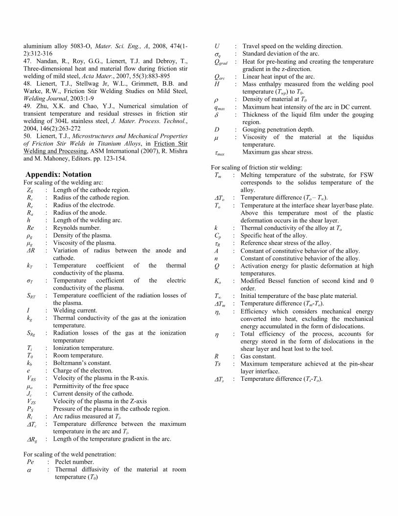
aluminium alloy 5083-O, Mater. Sci. Eng., A, 2008, 474(1-2):312-316 47. Nandan, R., Roy, G.G., Lienert, T.J. and Debroy, T., Three-dimensional heat and material flow during friction stir welding of mild steel, Acta Mater., 2007, 55(3):883-895 48. Lienert, T.J., Stellwag Jr, W.L., Grimmett, B.B. and Warke, R.W., Friction Stir Welding Studies on Mild Steel, Welding Journal, 2003:1-9 49. Zhu, X.K. and Chao, Y.J., Numerical simulation of transient temperature and residual stresses in friction stir welding of 304L stainless steel, J. Mater. Process. Technol., 2004, 146(2):263-272 50. Lienert, T.J., Microstructures and Mechanical Properties of Friction Stir Welds in Titanium Alloys, in Friction Stir Welding and Processing, ASM International (2007), R. Mishra and M. Mahoney, Editors. pp. 123-154. Appendix: Notation For scaling of the welding arc:
ZS : Length of the cathode region. Rc : Radius of the cathode region. Re : Radius of the electrode. Ra : Radius of the anode. h : Length of the welding arc. Re : Reynolds number. ρg : Density of the plasma. μg : Viscosity of the plasma. ΔR : Variation of radius between the anode and
cathode. kT : Temperature coefficient of the thermal
conductivity of the plasma. σT : Temperature coefficient of the electric
conductivity of the plasma. SRT : Temperature coefficient of the radiation losses of
the plasma. I : Welding current. kg : Thermal conductivity of the gas at the ionization
temperature. SRg : Radiation losses of the gas at the ionization
temperature Ti : Ionization temperature. T0 : Room temperature. kb : Boltzmann’s constant. e : Charge of the electron. VRS : Velocity of the plasma in the R-axis. μo : Permittivity of the free space Jc : Current density of the cathode. VZS Velocity of the plasma in the Z-axis PS Pressure of the plasma in the cathode region. Ri : Arc radius measured at Ti. ΔTc : Temperature difference between the maximum
temperature in the arc and Ti. ΔRg : Length of the temperature gradient in the arc.
For scaling of the weld penetration:
Pe : Peclet number. α : Thermal diffusivity of the material at room
temperature (T0)
U : Travel speed on the welding direction. σq : Standard deviation of the arc. Qgrad : Heat for pre-heating and creating the temperature
gradient in the z-direction. Qarc : Linear heat input of the arc. H : Mass enthalpy measured from the welding pool
temperature (Twp) to T0. ρ : Density of material at T0 qmax : Maximum heat intensity of the arc in DC current. δ : Thickness of the liquid film under the gouging
region. D : Gouging penetration depth. μ : Viscosity of the material at the liquidus
temperature. τmax Maximum gas shear stress.
For scaling of friction stir welding:
Tm : Melting temperature of the substrate, for FSW corresponds to the solidus temperature of the alloy.
ΔTo : Temperature difference (To – T∞). To : Temperature at the interface shear layer/base plate.
Above this temperature most of the plastic deformation occurs in the shear layer.
k : Thermal conductivity of the alloy at To Cp : Specific heat of the alloy. τR : Reference shear stress of the alloy. A : Constant of constitutive behavior of the alloy. n Constant of constitutive behavior of the alloy. Q : Activation energy for plastic deformation at high
temperatures. Ko : Modified Bessel function of second kind and 0
order. T∞ : Initial temperature of the base plate material. ΔTm : Temperature difference (Tm-To). ηs : Efficiency which considers mechanical energy
converted into heat, excluding the mechanical energy accumulated in the form of dislocations.
η : Total efficiency of the process, accounts for energy stored in the form of dislocations in the shear layer and heat lost to the tool.
R : Gas constant. Ts : Maximum temperature achieved at the pin-shear
layer interface. ΔTs : Temperature difference (Ts-To).


![[Welding] Weld Calculation](https://img.dokumen.tips/doc/110x75/577ce4a51a28abf1038ed313/welding-weld-calculation.jpg)