Scaling Laws for Heterogeneous Wireless Networks

by

Urs Niesen

Submitted to the Department of Electrical Engineering and ComputerScience

in partial fulfillment of the requirements for the degree of

Doctor of Philosophy

at the

MASSACHUSETTS INSTITUTE OF TECHNOLOGY

September 2009

c© Massachusetts Institute of Technology 2009. All rights reserved.

Author . . . . . . . . . . . . . . . . . . . . . . . . . . . . . . . . . . . . . . . . . . . . . . . . . . . . . . . . . . . . . .Department of Electrical Engineering and Computer Science

August 14, 2009

Certified by. . . . . . . . . . . . . . . . . . . . . . . . . . . . . . . . . . . . . . . . . . . . . . . . . . . . . . . . . .Devavrat Shah

Associate ProfessorThesis Supervisor

Certified by. . . . . . . . . . . . . . . . . . . . . . . . . . . . . . . . . . . . . . . . . . . . . . . . . . . . . . . . . .Gregory W. Wornell

Professor

Thesis Supervisor

Accepted by . . . . . . . . . . . . . . . . . . . . . . . . . . . . . . . . . . . . . . . . . . . . . . . . . . . . . . . . .

Terry P. OrlandoChairman, Department Committee on Graduate Students

2

Scaling Laws for Heterogeneous Wireless Networks

by

Urs Niesen

Submitted to the Department of Electrical Engineering and Computer Scienceon August 14, 2009, in partial fulfillment of the

requirements for the degree ofDoctor of Philosophy

Abstract

This thesis studies the problem of determining achievable rates in heterogeneous wire-less networks. We analyze the impact of location, traffic, and service heterogeneity.Consider a wireless network with n nodes located in a square area of size n commu-nicating with each other over Gaussian fading channels. Location heterogeneity ismodeled by allowing the nodes in the wireless network to be deployed in an arbitrarymanner on the square area instead of the usual random uniform node placement. Fortraffic heterogeneity, we analyze the n × n dimensional unicast capacity region. Forservice heterogeneity, we consider the impact of multicasting and caching. This givesrise to the n× 2n dimensional multicast capacity region and the 2n × n dimensionalcaching capacity region. In each of these cases, we obtain an explicit information-theoretic characterization of the scaling of achievable rates by providing a converseand a matching (in the scaling sense) communication architecture.

Thesis Supervisor: Devavrat ShahTitle: Associate Professor

Thesis Supervisor: Gregory W. WornellTitle: Professor

3

4

Acknowledgments

Many people have helped me with this thesis and throughout my time at MIT. First,

I would like to thank my two advisors, Devavrat Shah and Greg Wornell. I had the

good fortune to be advised by two individuals that truly cared about my development

— both professional as well as personal — and I learned a lot from both of them.

Further thanks go to Lizhong Zheng for agreeing to serve on my thesis committee.

I am also grateful to Piyush Gupta and Mitch Trott for hosting me during my

internships at Bell Labs and HP Labs, respectively. Further thanks go to Uri Erez,

Olivier Leveque, Sanjoy Mitter, Aslan Tchamkerten, Emre Telatar, and David Tse

for their influence during various stages of this research.

Thanks go also to the administrative staff of LIDS and SIA, and in particular Tricia

O’Donnell and Lynne Dell. Their help throughout these years is much appreciated.

My time in Cambridge would not have been the same without my friends and

colleagues at MIT. In particular, I would like to thank Anthony Accardi, Emmanuel

Abbe, Shashi Borade, Venkat Chandar, Venkat Chandrasekaran, Vijay Divi, Vishal

Doshi, Ying-zong Huang, Ashish Khisti, Minji Kim, Yuval Kochman, James Krieger,

Evgeny Logvinov, Baris Nakiboglu, Mesrob Ohannessian, Parikshit Shah, Maryam

Modir Shanechi, Charles Swannack, Katy Thorn, Kush Varshney, Lav Varshney, Da

Wang. Finally, I would like to thank my parents and Preeti Kamakoti for their love

and support when I needed it most.

This research was supported, in part, by the National Science Foundation under

Grant No. CCF-0635191, by DARPA under Grant No. 18870740-37362-C, and by

Hewlett-Packard under the MIT/HP Alliance. This funding is greatly appreciated.

5

6

Contents

1 Introduction 9

1.1 Network Models . . . . . . . . . . . . . . . . . . . . . . . . . . . . . . 11

1.2 Prior Work . . . . . . . . . . . . . . . . . . . . . . . . . . . . . . . . 13

1.3 Thesis Outline . . . . . . . . . . . . . . . . . . . . . . . . . . . . . . . 21

2 Network Model and Notation 29

2.1 Notation and Conventions . . . . . . . . . . . . . . . . . . . . . . . . 29

2.2 Network Model . . . . . . . . . . . . . . . . . . . . . . . . . . . . . . 30

2.3 Capacity Regions . . . . . . . . . . . . . . . . . . . . . . . . . . . . . 32

3 Location Heterogeneity 41

3.1 Main Results . . . . . . . . . . . . . . . . . . . . . . . . . . . . . . . 42

3.2 Hierarchical Relaying Scheme . . . . . . . . . . . . . . . . . . . . . . 48

3.3 Cooperative Multi-Hop Scheme . . . . . . . . . . . . . . . . . . . . . 61

3.4 Analysis of the Hierarchical Relaying Scheme . . . . . . . . . . . . . . 63

3.5 Proof of Achievability (α ∈ (2, 3]) . . . . . . . . . . . . . . . . . . . . 80

3.6 Proof of Converse (α ∈ (2, 3]) . . . . . . . . . . . . . . . . . . . . . . 91

3.7 Proof of Adversarial Optimality of Hierarchical Relaying (α > 3) . . . 95

3.8 Proof of Achievability (α > 3) . . . . . . . . . . . . . . . . . . . . . . 96

3.9 Proof of Converse (α > 3) . . . . . . . . . . . . . . . . . . . . . . . . 100

3.10 Discussion . . . . . . . . . . . . . . . . . . . . . . . . . . . . . . . . . 101

3.11 Chapter Summary . . . . . . . . . . . . . . . . . . . . . . . . . . . . 105

7

4 Traffic Heterogeneity 107

4.1 Main Results . . . . . . . . . . . . . . . . . . . . . . . . . . . . . . . 108

4.2 Example Scenarios . . . . . . . . . . . . . . . . . . . . . . . . . . . . 115

4.3 Communication Scheme for Unicast Traffic . . . . . . . . . . . . . . . 119

4.4 Auxiliary Lemmas . . . . . . . . . . . . . . . . . . . . . . . . . . . . 123

4.5 Proof of Inner Bound . . . . . . . . . . . . . . . . . . . . . . . . . . . 138

4.6 Proof of Outer Bound . . . . . . . . . . . . . . . . . . . . . . . . . . 148

4.7 Discussion . . . . . . . . . . . . . . . . . . . . . . . . . . . . . . . . . 148

4.8 Chapter Summary . . . . . . . . . . . . . . . . . . . . . . . . . . . . 152

5 Service Heterogeneity: Multicast 155

5.1 Main Results . . . . . . . . . . . . . . . . . . . . . . . . . . . . . . . 156

5.2 Example Scenarios . . . . . . . . . . . . . . . . . . . . . . . . . . . . 161

5.3 Communication Scheme for Multicast Traffic . . . . . . . . . . . . . . 163

5.4 Proofs . . . . . . . . . . . . . . . . . . . . . . . . . . . . . . . . . . . 165

5.5 Discussion . . . . . . . . . . . . . . . . . . . . . . . . . . . . . . . . . 169

5.6 Chapter Summary . . . . . . . . . . . . . . . . . . . . . . . . . . . . 171

6 Service Heterogeneity: Caching 173

6.1 Main Results . . . . . . . . . . . . . . . . . . . . . . . . . . . . . . . 174

6.2 Example Scenarios . . . . . . . . . . . . . . . . . . . . . . . . . . . . 178

6.3 Communication Scheme for Caching Traffic . . . . . . . . . . . . . . . 182

6.4 Proofs . . . . . . . . . . . . . . . . . . . . . . . . . . . . . . . . . . . 183

6.5 Discussion . . . . . . . . . . . . . . . . . . . . . . . . . . . . . . . . . 203

6.6 Chapter Summary . . . . . . . . . . . . . . . . . . . . . . . . . . . . 205

7 Conclusions 207

7.1 Thesis Summary . . . . . . . . . . . . . . . . . . . . . . . . . . . . . 207

7.2 Future Work . . . . . . . . . . . . . . . . . . . . . . . . . . . . . . . . 209

8

Chapter 1

Introduction

Over the past decades, there has been a growing disconnect between the size of

communication networks that are built and planned and the size of communication

networks that are fundamentally understood. On the one hand, wireline networks

(like the Internet) have grown from only a few hundred users in 1981 to over one billion

in 2008, and wireless networks (like metropolitan mesh networks, sensor networks, or

military ad-hoc networks) with up to a million communication devices are being

envisioned. On the other hand, even simple communication networks, as for example

a four node wireless network with two sources and two destinations, or an even simpler

three node network with one source, one destination, and one relay, are only partially

understood. Central questions remain unanswered: What is the role of interference

in the four node example above, and what is the role of cooperation in the three node

example? An answer to these questions will undoubtedly have profound implications

on the design of future communication networks.

A main reason for this disconnect is that much of the effort analyzing these com-

munication systems has been directed at obtaining exact solutions for small networks

and trying to gain insight for larger networks from it. This has proved challenging,

as the lack of a complete understanding of even very simple networks like the ones

mentioned above illustrates. Another approach is to directly consider large networks,

but instead settle for an approximate asymptotic solution.

To analyze such large networks, a model of how they are generated has to be

9

chosen. More precisely, consider a wireless network with n nodes. How should the

location of these n nodes be chosen; how should the traffic demand they generate

behave; and how should the services they require be modeled? This question is usually

addressed by making several homogeneity assumptions. For the node locations, it is

usually assumed that nodes are placed uniformly at random on a square of area n;

for the traffic demands that each node is source for exactly one destination node

chosen uniformly at random from among all the other nodes, and that all these n

source-destination pairs communicate at equal rate; for the service requirements that

all nodes generate only unicast traffic.

While this homogeneous setting is convenient mathematically, it does not provide

a very accurate model of reality. In fact, for the node locations it is likely that some

areas are denser than others (e.g., towns vs. countryside); for the traffic demands

that users communicate to nearby nodes more often than to faraway ones, and that

some users will create more traffic than others (e.g., sending an email vs. streaming

a movie); for the service requirements that some information needs to be transmitted

to several or all nodes. In other words, we expect node location, traffic demands,

and service requirements to be highly heterogeneous. Moreover, these heterogeneities

will lead to different asymptotic behavior of the network. This implies that the

results obtained for large homogeneous wireless networks will only yield a limited

understanding of the heterogeneous networks we are likely to encounter in practice.

In this thesis, we develop approximate asymptotic characterizations of the perfor-

mance of large heterogeneous wireless networks. We consider the impact of location,

traffic, and service heterogeneity. The common approach to deal with these hetero-

geneities consists of first finding the underlying “coarse structure” of the network,

capturing the essential parts of the heterogeneity. Once such a simple coarse struc-

ture is identified, rather complicated questions about the network can be elegantly

analyzed by recasting them for the underlying coarse structure. Moreover, this coarse

structure allows to obtain insight into the role of interference or cooperation in large

networks and can guide the design of communication schemes and algorithms.

10

1.1 Network Models

As mentioned in the previous section, to analyze large networks a model for their

generation has to be chosen. Here we briefly review some popular such models used

throughout the literature.

First, a model for the node location needs to be chosen. A standard assumption

is that the n nodes of the wireless network are located on a square of area1 n. It is

often assumed that the nodes are placed uniformly and independently at random on

this square, which we refer to as random node placement. If nodes are allowed to be

placed in an arbitrary deterministic manner on this square, we speak of an arbitrary

node placement. In the case of arbitrary node placement, it is usually assumed that

there is some constant (independent of n) minimum separation between the nodes.

This minimum-separation requirement prevents degenerate node placements.

Second, a model for communication between these nodes needs to be selected.

There are two broad categories of such models. Models in the first category are

motivated by current wireless technology and are referred to as protocol models. We

describe two of them in more detail.

Protocol Model 1: Node v can receive data from node u at rate 1 bits/s if it lies

outside the region of interference of each other transmitter.

Protocol Model 2: Node v can receive data from node u at rate log(1 + SINR)

bits/s, where SINR is the signal to interference plus noise ratio at the receiving

node v. Here signals are attenuated as r−α/2 over distance r for some path-loss

exponent α > 2.

These communication models share two assumptions. First, they only allow point-to-

point communication, and second, they treat all interference as noise. In other words,

these models makes assumptions on the communication protocol used between these

1This is referred to as extended node placement. When nodes are located on a square of area 1for any n, we speak of a dense node placement. Results for the two cases are closely related, and wefocus on the extended case in this thesis.

11

nodes2. These two assumptions imply that the only allowed communication scheme

in the wireless network is multi-hop routing, in which a message travels over multiple

hops from its source to its destination, and each node along this route decodes the

message received from the previous node and then re-encodes it for the subsequent

one.

Models in the second category do not make any assumptions about the commu-

nication protocol used, but rather aim at directly describing the underlying wireless

channel. Two popular models are the following.

Gaussian Model: Signals transmitted at node u are received at node v at distance

r attenuated by a factor r−α/2 for some path-loss exponent α > 2, and then

further corrupted by additive Gaussian noise.

Gaussian Fading Model: Signals transmitted at node u are received at node v at

distance r attenuated by a factor r−α/2hu,v for some path-loss exponent α > 2,

and then further corrupted by additive Gaussian noise. Here hu,v models small-

scale fading between the nodes u and v, and is usually assumed to vary in a

stationary ergodic fashion across time.

Third, a choice of service requirements has to be made. The simplest such service

requirement is unicast traffic, in which each message is available at only one source

node and requested at only one destination node. When each message is only available

at one source node, but the same message may be requested by several destination

nodes, we speak of multicast traffic. The extreme case, in which each message needs to

be transmitted to all the nodes in the network, is termed broadcast traffic. Instead of

varying the number of destinations for a given message, we can also vary the number

of sources that have access to a given message. We think of these sources having

access to the same message as caches in the network, replicating these messages. If

several sources have access to the same message, but each such message needs to be

transmitted to only one destination node, we speak of caching traffic.

2More commonly, only the first model is called protocol model. The second model is usuallyreferred to as generalized physical model. We use the name protocol model for both of them tohighlight that they both make assumptions on the communication protocol used and to contrastthem with the more information-theoretic Gaussian fading channel models described in the following.

12

Fourth, a model for traffic generation is required. The standard assumption for

unicast traffic is that each node is source for exactly one other node, and this des-

tination node is chosen uniformly and independently at random from among all the

other nodes. Moreover, all these n source-destination pairs generate traffic at equal

rate. We refer to this as random source-destination pairing with uniform rate. The

corresponding maximal achievable per-node rate is called the throughput capacity of

the wireless network. Another figure of merit for unicast traffic that is often used

is the transport capacity, which is the maximum achievable rate-distance product,

summed over all source-destination pairs. General unicast traffic gives rise to the

unicast capacity region ΛUC(n) ⊂ Rn×n+ , which characterizes the set of achievable

rates for each of the possible n2 source-destination pairs. For multicast traffic the

standard homogeneity assumption is that each node in the network is a source and

requires to multicast at uniform rate to the same number of destination nodes chosen

uniformly at random. As before, general multicast traffic gives rise to the multicast

capacity region ΛMC(n) ⊂ Rn×2n

+ , which characterizes the set of achievable rates for

each of the possible n × 2n pairs of source and corresponding group of destinations.

Finally, achievable general caching traffic can be described by the caching capacity

region ΛCA(n) ⊂ R2n×n+ , which characterizes the set of achievable rates for each of the

possible 2n × n pairs of caches and corresponding destination.

1.2 Prior Work

In this section, we review prior work on scaling laws for wireless networks. Most

of the literature on the subject focuses on the homogeneous setting, i.e., random

node placement and unicast traffic under random source-destination pairing with

uniform rate. The literature pertaining to this homogeneous setting is surveyed in

Section 1.2.1. The literature for arbitrary node placement, in which no probabilistic

assumptions are made on the node location, is reviewed in Section 1.2.2. Prior work

considering more general unicast traffic patterns is discussed in Section 1.2.3. Finally,

Section 1.2.4 provides a literature survey for work on service heterogeneity, such as

13

multicast, broadcast, and caching traffic.

1.2.1 Homogeneous Setting

The scaling approach to analyzing wireless networks was pioneered by Gupta and

Kumar in [15]. They show that under random node placement and assuming protocol

model 1, the throughput capacity scales like3 Θ((n log(n))−1/2

). For protocol model

2, they prove an upper bound of O(n−1/α

), and a lower bound of Ω

((n log(n))−1/2

)

(see also [14]). Achievability (i.e., the lower bound on the throughput capacity)

is shown using a straight-line multi-hop routing scheme. For protocol model 1, a

simpler proof of the Ω((n log(n))−1/2

)lower bound on the throughput capacity was

provided subsequently in [30]. Achievability is shown there by multi-hop routing

along a grid structure instead of straight line routing proposed in [15]. Using an

argument in [3] relating protocol models 1 and 2, the communication scheme proposed

in [30] also applies to protocol model 2. The upper bound for protocol model 2 was

later sharpened to O(n−1/2

)in [3]. This leaves only a order log−1/2(n) gap between

the upper and lower bounds for protocol model 2. This gap was closed in [10],

where it is shown that, under protocol model 2, the throughput capacity scales like

Θ(n−1/2

). To summarize, under protocol model 1 the throughput capacity scales like

Θ((n log(n))−1/2

), and under protocol model 2 the throughput capacity scales like

Θ(n−1/2

).

The results mentioned in the last paragraph show that under a protocol model

assumption, the maximum achievable per-node rate with random source-destination

pairing decays to zero essentially as Θ(n−1/2

). However, this result was derived by

restricting communication schemes to just multi-hop routing (by making the proto-

col model assumption). While such a restriction is motivated by current technology,

it is not clear that multi-hop communication is optimal for large wireless networks.

To make claims about the performance of wireless networks under any communica-

tion scheme, a more information-theoretic approach using a Gaussian channel model

(either with or without fading) is necessary.

3We use Knuth’s asymptotic notation. See Section 2.1 for a formal definition.

14

Since any communication scheme for the protocol models is also a communication

scheme for the Gaussian channel models achieving the same order rate, we obtain from

the results mentioned above that under both Gaussian channel models (i.e., with or

without fading) throughput capacity is lower bounded by Ω(n−1/2

). The work on

scaling laws under the Gaussian channel models can be grouped into two streams.

One stream of work [4, 21, 32, 37, 38, 48, 50, 51] focused on progressively broadening

the conditions on the channel model, under which multi-hop communication is indeed

order optimal, and hence throughput capacity is also upper bounded by O(n−1/2

).

Another stream of work [1,16,28,38,49] focused on progressively more refined multi-

user cooperative schemes, which are shown to significantly out-perform multi-hop

communication in certain environments, hence improving the Ω(n−1/2

)lower bound

on the throughput capacity.

For the upper bounds, it was argued in [48] that for the Gaussian channel model

with path-loss exponents α > 6 (i.e., signal power decays quickly as a function of

distance), throughput capacity is upper bounded by O(n−1/2

), and hence multi-hop

communication is order optimal in this regime. This result was later extended for

the Gaussian fading channel model in [51]. A sharper bound was found subsequently

in [21], where it is shown that under both Gaussian channel models (with or without

fading), the same upper bound holds for α > 5. In [32] it is shown that under

a Gaussian channel model, even for α ∈ (2, 5] the throughput capacity is upper

bounded by O(n1/α−1/2 log(n)

). While this does not prove the order optimality of

multi-hop communication, it does show that the throughput capacity must decay

to zero as n → ∞. The threshold above which multi-hop communication is order

optimal was further reduced to α > 4.5 in [4], and to α > 4 in [50] for both Gaussian

channel models. For the Gaussian fading channel model, it is shown in [38] that the

throughput capacity is O(n−1/2+ε

)for α > 3 and O

(n1−α/2+ε

)for α ∈ (2, 3] for any

ε > 0. Hence multi-hop is order optimal in the sense of achieving the best scaling

exponent for α > 3. For the Gaussian channel model without fading, [37] shows that

for α ∈ (2, 4], throughput capacity is upper bounded by O(n1/(α+8)−1/2 log3(n)

). All

these results rely on the cut-set bound to upper bound the sum rate across a cut

15

by the capacity of a multiple-input multiple-output (MIMO) point-to-point channel

in which all the nodes on one side of the cut are allowed to cooperate in sending

a message and all nodes on the other side of the cut are allowed to cooperate in

receiving this message. They differ, however, in their analysis of this MIMO channel.

For the lower bounds, it was first argued in [16] that there exists a (carefully con-

structed) node placement such that under either Gaussian channel model (i.e., with

or without fading) higher rates than suggested by the results for the protocol models

are achievable. This node placement consists of two clusters each containing half the

nodes. In the communication scheme proposed in [16], the nodes in the first cluster

exchange all their messages among themselves and then jointly encode and transmit

them. The first part can be carried out efficiently since the all the nodes are located

close to each other. Similarly, the nodes in the second cluster exchange their received

observations and then jointly decode them. This procedure effectively transforms the

network into a distributed MIMO channel. Similar distributed cooperative schemes

were also suggested in [28, 49]. While the results in [16] hold only for a particular

node placement, it is shown in [1] that a similar approach can also be used under

random node placement. However, since the nodes are now less clustered, setting up

the distributed MIMO channel incurs a loss. In [38] it is shown that this loss can

be circumvented by using the scheme proposed in [1] multiple times in a hierarchical

fashion. More precisely, the problem of setting up the distributed MIMO channel is

recognized as being essentially the same as the original communication problem, but

at a smaller scale. Using the same scheme recursively, we can thus reduce this scale

to a point where the penalty of setting up the initial distributed MIMO channel is

negligible. Analyzing this scheme yields that for the Gaussian fading channel model

and α ∈ (2, 3), the throughput capacity is lower bounded by Ω(n1−α/2−ε

)for any

ε > 0. This matches the upper bound derived in the same paper up to ε (see the

previous paragraph), and hence establishes that the throughput capacity scales like

Θ(n1−α/2±ε

)in this regime.

To summarize, under the Gaussian channel model with fading, the throughput

scales essentially like Θ(n1−min3,α/2±ε

)for any α > 2 (with improvements on the ±ε

16

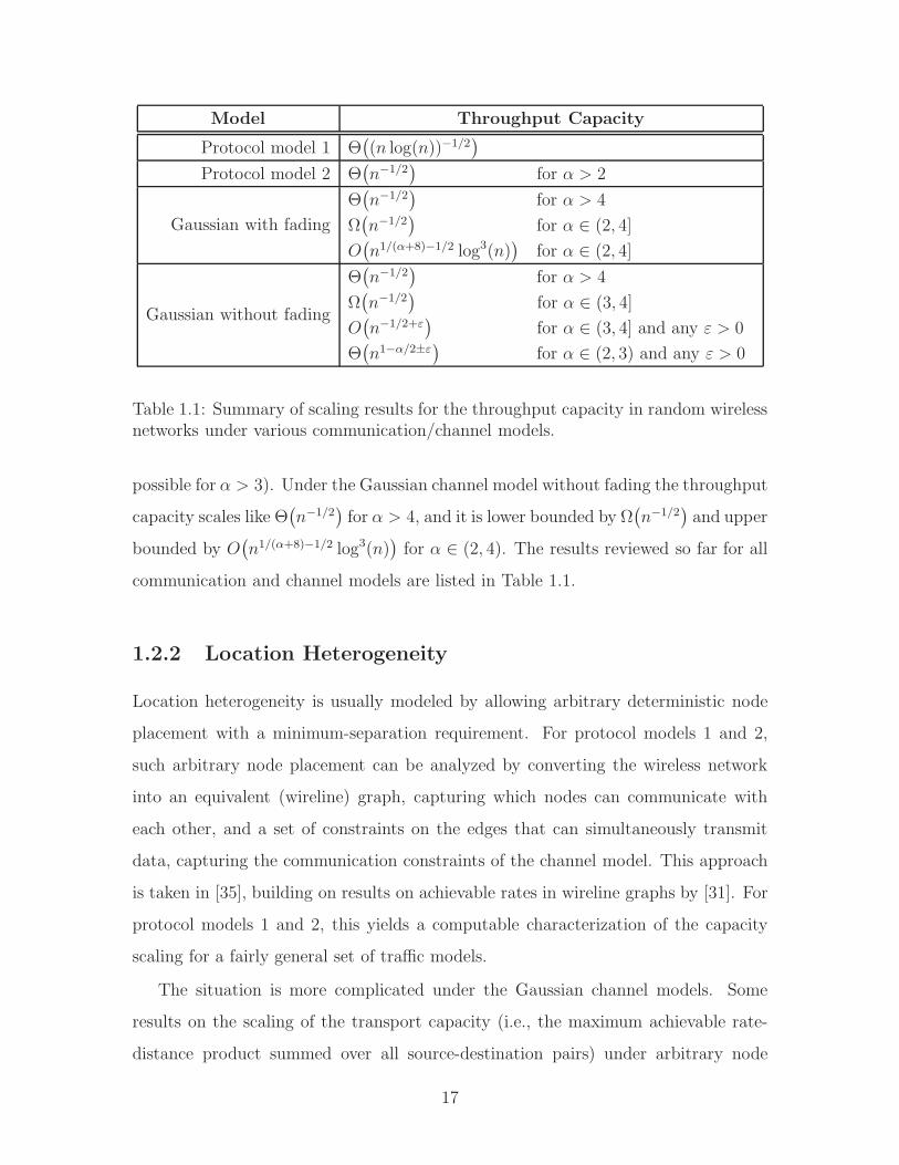
Model Throughput Capacity

Protocol model 1 Θ((n log(n))−1/2

)

Protocol model 2 Θ(n−1/2

)for α > 2

Gaussian with fading

Θ(n−1/2

)for α > 4

Ω(n−1/2

)for α ∈ (2, 4]

O(n1/(α+8)−1/2 log3(n)

)for α ∈ (2, 4]

Gaussian without fading

Θ(n−1/2

)for α > 4

Ω(n−1/2

)for α ∈ (3, 4]

O(n−1/2+ε

)for α ∈ (3, 4] and any ε > 0

Θ(n1−α/2±ε

)for α ∈ (2, 3) and any ε > 0

Table 1.1: Summary of scaling results for the throughput capacity in random wirelessnetworks under various communication/channel models.

possible for α > 3). Under the Gaussian channel model without fading the throughput

capacity scales like Θ(n−1/2

)for α > 4, and it is lower bounded by Ω

(n−1/2

)and upper

bounded by O(n1/(α+8)−1/2 log3(n)

)for α ∈ (2, 4). The results reviewed so far for all

communication and channel models are listed in Table 1.1.

1.2.2 Location Heterogeneity

Location heterogeneity is usually modeled by allowing arbitrary deterministic node

placement with a minimum-separation requirement. For protocol models 1 and 2,

such arbitrary node placement can be analyzed by converting the wireless network

into an equivalent (wireline) graph, capturing which nodes can communicate with

each other, and a set of constraints on the edges that can simultaneously transmit

data, capturing the communication constraints of the channel model. This approach

is taken in [35], building on results on achievable rates in wireline graphs by [31]. For

protocol models 1 and 2, this yields a computable characterization of the capacity

scaling for a fairly general set of traffic models.

The situation is more complicated under the Gaussian channel models. Some

results on the scaling of the transport capacity (i.e., the maximum achievable rate-

distance product summed over all source-destination pairs) under arbitrary node

17

placement are known. In [48], it is shown that under such node placement and using a

Gaussian channel model without fading, the transport capacity is upper bounded by

O(n) for α > 6. For Gaussian fading channels, the same behavior was shown to hold

for α > 6 in [51]. Under both Gaussian channel models the same O(n) upper bound

on the transport capacity was argued to hold for α > 5 in [21], for α > 4.5 in [4], and

for α > 4 in [50]. Matching lower bounds are, however, usually only available under

stricter conditions on the node placement. In [51], it is shown that the transport

capacity is also lower bounded by Ω(n) for any α > 2 if the node placement is such

that for every node at least one other node is within distance Θ(1). The unicast

traffic that achieves this lower bound pairs each node with its nearest neighbor into

a source-destination pair, and all these n pairs communicate at equal rate.

1.2.3 Traffic Heterogeneity

As mentioned in the previous section, under protocol models 1 or 2, the wireless net-

work can be transformed into an equivalent wireline graph. This is used in [35] to

analyze more general traffic patterns. The authors consider product multicommodity

flows, in which each source-destination pair (u, v) wants to communicate at rate πuπv,

where πu are arbitrary nonnegative numbers. For such traffic patterns, achievable

rates scale like the conductance of the equivalent wireline graph [35]. Another ap-

proach is to consider the transport capacity of the wireless network. The transport

capacity upper bounds every achievable rate-distance product summed over all source-

destination pairs. As such it provides an upper bound on the transport rate for any

achievable unicast traffic matrix. In other words, the transport capacity provides a

hyperplane that contains the capacity region and origin on the same side. Through a

repeated application of this transport capacity bound at different scales, [42, 43] ob-

tained an implicit characterization of the unicast capacity region under a simplified

version of protocol model 1. Achievability is shown in [43] using a localized variant

of the two-phase Valiant-Brebner routing scheme developed in [47].

For the Gaussian channel models, asymptotic upper bounds on the transport ca-

pacity were obtained in [21,48,50,51]. However, as was discussed in the last paragraph,

18

the transport capacity provides only partial information about the unicast capacity re-

gion. Generalized transport capacities, in which the rate between a source-destination

pair at distance r is weighted by f(r) for some function f are analyzed in [4]. These

generalized transport capacities provide tighter outer bounds on the unicast capacity

region.

1.2.4 Service Heterogeneity

So far, we have discussed only unicast traffic. More general service requirements

(such as broadcast, multicast, or caching traffic) have recently attracted attention.

In [46], broadcasting under (a simplified version of) protocol model 1 is studied. It is

shown that under random node placement the maximal per-node rate at which every

node can simultaneously broadcast information in the network is upper bounded

by O(n−1). The same problem is analyzed under protocol model 2 in [52], and it is

shown that the maximal achievable per-node rate scales like Θ(n−1 log−α/2(n)

). More

general broadcast traffic, in which each node broadcasts data at different (possibly

zero) rates, have been studied in [23, 24], where it is shown that general broadcast

traffic is achievable if and only if its sum rate scales like Θ(1)

for protocol model 1 or

like Θ(log−α/2(n)

)for protocol model 2. In other words, the only relevant quantity

when analyzing broadcast traffic is the sum rate. This is because the broadcast

requirement induces a uniform received traffic pattern, even if the transmitted traffic

pattern is not (i.e., all nodes are required to receive information at the same rate). An

information-theoretic approach to the problem was taken in [40] to analyze broadcast

from a single source under random node placement and assuming a Gaussian fading

channel model. The maximal achievable broadcast rate for the source is shown to

be upper bounded by O(log log(n)

)and lower bounded by Ω(1). Achievability (i.e.,

the lower bound) is proved using a cooperative multistage scheme. In the first stage,

the message is transmitted by the source. In the second stage, nodes that were

able to decode the sent message successfully, cooperatively retransmit the message.

The scheme continues in the same fashion until all nodes have correctly decoded the

message. Similar cooperative schemes for broadcast over Gaussian fading channels

19

have also been studied in [19, 26].

The analysis of multicast traffic is considerably more difficult. For random node

placement and protocol model 1, the maximal uniformly achievable per-node rate for

multicast from nβ (with β ∈ (0, 1)) randomly selected source nodes to the remaining

n1−β nodes in the network has been shown to scale like Θ((nβ log(n))−1/2

)in [39].

Under the same assumptions (but with a simplified variant of protocol model 1), it

was shown in [33] that when each node wants to multicast at uniform rate to nβ (with

β ∈ (0, 1)) randomly chosen destinations, the maximal achievable per-node rate scales

like Θ((n1+β log(n))−1/2

). This was subsequently generalized to protocol model 2 by

[25], where it is shown that under the same traffic and node placement assumptions as

in [33], the maximal achievable per node-rate scales like Θ((n1+β)−1/2

). Achievability

in [25] is shown using the scheme of [10], and the same log−1/2(n) gap can be observed

between the results for protocol models 1 and 2, just as in the unicast case. To the

best of our knowledge, the scaling of achievable multicast rates has not been studied

from an information-theoretic point of view using either of the Gaussian channel

models.

The analysis of caching traffic can be separated into two distinct problems. In

the cache selection problem, we are given a set of caches and are interested in op-

timally selecting caches for each destination node and the resulting performance of

the network. In the cache placement problem, we are interested in optimally placing

the caches in order to maximize the performance of the network. Most of the prior

work on caching focuses on the second problem and sidesteps the first one by making

two assumptions. First, the wireless network is modeled by a (possibly capacitated)

graph, and second, each destination node requests the entire message from the closest

(with respect to the graph distance) node. For arbitrary graphs, the cache placement

problem can then be formulated as a variant of the classical facility location problem

(see, e.g., [6, 29] and references therein). In the context of wireless networks, this

problem has been studied in [5, 20, 27, 36, 44, 45], with the wireless network modeled

as a graph induced by a simplified version of protocol model 1. More precisely, con-

stant factor approximation algorithms for optimal cache placement for one message

20

under different communication constraints are proposed in [36, 44]. Constant factor

approximation algorithms for multiple messages under different memory constraints

are proposed in [27,45]. Scaling results for the cache placement problem are presented

in [20], which derives asymptotically optimal cache densities assuming random node

placement and uniform traffic, and in [5], which analyzes the resulting scaling of

achievable rates. As mentioned before, the results on caching traffic surveyed in this

paragraph model the wireless network as a graph and assume nearest-neighbor cache

selection. Hence they address only the cache placement problem while avoiding the

cache selection problem.

Caching in wireless networks has not been directly considered in the information

theory literature. However, it can be seen that the cache selection problem is a

special case of the problem of communicating correlated sources over a noisy network.

Indeed, we can consider that each cache has an identical message to send to the same

destination. The more general problem of transmitting correlated sources over noisy

networks has received considerable attention. Unlike the situation with point-to-point

communication, for network communication problems source-channel separation does

not hold in general [8]. Hence, the problem of source and channel coding have to be

considered jointly. While for some special cases optimal communication strategies

for transmitting correlated sources over a noisy network are known (for example,

broadcast from a single source with independent network links [7, 17]), the general

problem is unsolved.

1.3 Thesis Outline

This thesis considers the impact of different heterogeneities on achievable rates in a

wireless network. Throughout, we assume the Gaussian fading channel model. Our

treatment is information theoretic and hence allows claims to be made about the

performance of wireless networks under any communication scheme consistent with

the model.

21

1.3.1 Location Heterogeneity

As mentioned earlier, the standard homogeneity assumption for the location of nodes

is that they are placed independently and uniformly at random on a square of area n.

However, in many situations this might not be a good model of reality. A more general

assumption is to allow for arbitrary node placement with a constant (independent of

n) minimum separation between nodes. We adopt this model to study the effect

of location heterogeneity on the scaling of achievable rates. To study this effect in

isolation, we keep the homogeneity assumptions for traffic and service requirements,

i.e., we assume unicast traffic induced by random source-destination pairing with

uniform rate.

Several complications arise due to the introduction of location heterogeneity. As

we have seen in Section 1.2.1, in the homogeneous case the optimal communica-

tion scheme depends crucially on the path-loss exponent α: For α ≥ 3, multi-hop

communication is order optimal, whereas for α ∈ (2, 3] hierarchical cooperative com-

munication is order optimal. The first complication is that under arbitrary node

placement these schemes might either be clearly suboptimal or not even be imple-

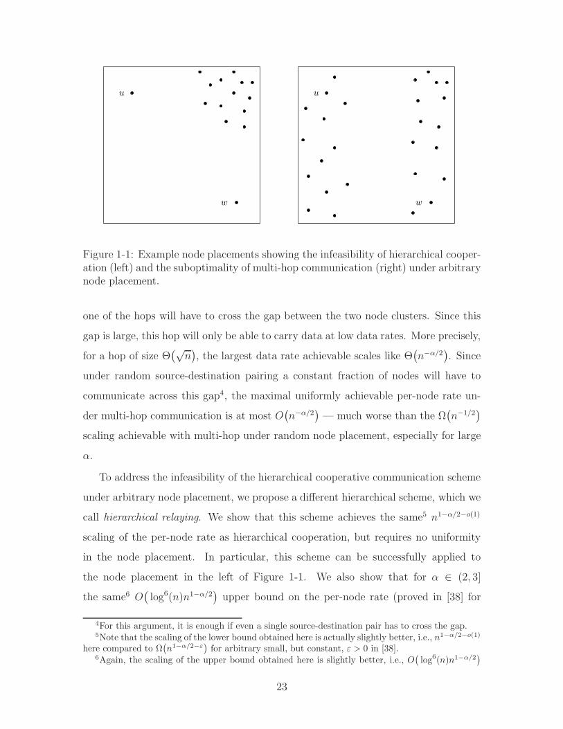
mentable at all. As an example, consider the two node placements in Figure 1-1. The

left node placement shows infeasibility of hierarchical cooperation under arbitrary

node placement. Recall from Section 1.2.1 that the hierarchical cooperation scheme

operates by setting up distributed MIMO transmitter and receiver clusters at increas-

ingly bigger scales. In other words, the neighbors of each source help transmitting,

and the neighbors of each destination help receiving the message. Consider now the

source-destination pair (u, w) in the left node placement in Figure 1-1. These nodes

are both isolated, i.e., they have no immediate neighbors. Hence neither the trans-

mitter MIMO cluster nor the receiver MIMO cluster can be effectively constructed.

The right node placement shows suboptimality of multi-hop communication. In this

example, half of the nodes are placed on the left of the square area, the other half on

the right. The gap between these two node clusters is of order Θ(√

n). Consider the

source-destination pair (u, w) in this figure. For a multi-hop communication scheme,

22

w

u

w

u

Figure 1-1: Example node placements showing the infeasibility of hierarchical cooper-ation (left) and the suboptimality of multi-hop communication (right) under arbitrarynode placement.

one of the hops will have to cross the gap between the two node clusters. Since this

gap is large, this hop will only be able to carry data at low data rates. More precisely,

for a hop of size Θ(√

n), the largest data rate achievable scales like Θ

(n−α/2

). Since

under random source-destination pairing a constant fraction of nodes will have to

communicate across this gap4, the maximal uniformly achievable per-node rate un-

der multi-hop communication is at most O(n−α/2

)— much worse than the Ω

(n−1/2

)

scaling achievable with multi-hop under random node placement, especially for large

α.

To address the infeasibility of the hierarchical cooperative communication scheme

under arbitrary node placement, we propose a different hierarchical scheme, which we

call hierarchical relaying. We show that this scheme achieves the same5 n1−α/2−o(1)

scaling of the per-node rate as hierarchical cooperation, but requires no uniformity

in the node placement. In particular, this scheme can be successfully applied to

the node placement in the left of Figure 1-1. We also show that for α ∈ (2, 3]

the same6 O(log6(n)n1−α/2

)upper bound on the per-node rate (proved in [38] for

4For this argument, it is enough if even a single source-destination pair has to cross the gap.5Note that the scaling of the lower bound obtained here is actually slightly better, i.e., n1−α/2−o(1)

here compared to Ω(n1−α/2−ε

)for arbitrary small, but constant, ε > 0 in [38].

6Again, the scaling of the upper bound obtained here is slightly better, i.e., O(log6(n)n1−α/2

)

23

the homogeneous case) is also valid under arbitrary node placement. Together, this

answers the question of scaling of the throughput capacity under arbitrary node

placement for the low path-loss exponent regime α ∈ (2, 3].

As we argued in the last paragraph, for α ∈ (2, 3] the node placement has no im-

pact on the scaling performance. The situation is markedly different for large path-loss

exponent α > 3. We introduce a regularity parameter, measuring on a coarse level the

uniformity of the node placement. We show how the scaling of throughput capacity

depends on this regularity parameter. The proposed order optimal communication

scheme smoothly “interpolates” from multi-hop communication (which is order opti-

mal under uniform node placement) to hierarchical relaying (which is order optimal

under completely irregular node placement) depending on this regularity parameter.

As an example, we show that for the node placement on the right in Figure 1-1, the

order optimal communication scheme is hierarchical relaying, achieving a per-node

rate of n1−α/2−o(1). This contrasts with the performance of multi-hop communication,

which is yields a per-node rate of at most O(n−α/2

).

As mentioned in the introduction, the common approach to deal with hetero-

geneities consists of identifying the underlying “coarse structure” of the network,

capturing the essential parts of the heterogeneity. The coarse structure of the wire-

less network in this case (for α > 3) is a wireline noiseless grid graph where each node

in the grid corresponds to a cluster of nodes in the wireless network with cluster size

depending on the regularity of the node placement. This coarse structure explicitly

captures the amount of cooperation that is required as a function of the regularity of

the node placement.

Location heterogeneity is discussed in detail in Chapter 3.

1.3.2 Traffic Heterogeneity

As was discussed in Section 1.1, the standard homogeneity assumption for traffic

generation is that each node is source exactly once and wants to transmit data at

uniform rate to a destination node chosen uniformly at random from among the other

here compared to O(n1−α/2+ε

)for any (constant) ε > 0 in [38].

24

nodes. This kind of traffic pattern has several problematic characteristics. The first

one is uniformity of traffic (i.e., all source-destination pairs want to communicate at

the same rate). Most traffic patterns observed in large networks (say the Internet)

are quite different, in that they have a large number of users generating little traffic,

and a small number of users generating a lot of traffic. Traffic variations of this kind

are not captured by the homogeneous traffic assumption. The second characteristic of

the homogeneous traffic assumption is that, since each node chooses a destination at

random, most source-destination pairs will be at a distance of Θ(√

n). This is again

unlike the situation in actual networks where communication patterns are likely to

be more localized. The third characteristic of such traffic patterns is that each node

is source exactly once and is destination at most a few times. Situations in which we

have a server that needs to transmit data to many nodes, or a user downloading data

from many other nodes cannot be accommodated under this assumption.

To overcome these limitations, we turn to general unicast traffic. In other words,

we are interested in the entire unicast capacity region ΛUC(n) ⊂ Rn×n+ . To study

the effect of traffic heterogeneity in isolation, we assume random node placement.

As always, we assume a Gaussian fading channel model. While outer bounds on

the unicast capacity region ΛUC(n) can be derived from results on transport capacity

reviewed in Section 1.2.2, these bounds are quite simple in that they only provide

one hyperplane containing the capacity region and the origin on one side, and they

do not provide a scaling characterization of ΛUC(n). The situation is worse for inner

bounds, where except for some special points (as the one resulting from homogeneous

traffic) not much is known.

In this thesis, we find inner and outer bounds on the n2-dimensional unicast

capacity region. These bounds behave asymptotically in the same way along at least

n2 − n of the total n2 dimensions for α ∈ (2, 5], and for all n2 dimensions for α > 5.

Hence they determine the scaling behavior of either most (for α ∈ (2, 5]) or all (for

α > 5) of the unicast capacity region ΛUC(n). More precisely, we define two sets

ΛUC1 (n), ΛUC

2 (n) ⊂ Rn×n+ , coinciding along at least n2 − n dimensions. We show that

25

for α ∈ (2, 5],

n−o(1)ΛUC

1 (n) ⊂ ΛUC(n) ⊂ O(log6(n))ΛUC

2 (n),

and for α > 5,

n−o(1)ΛUC

1 (n) ⊂ ΛUC(n) ⊂ O(log6(n))ΛUC

1 (n).

In words, for α > 5, if we shrink ΛUC1 (n) by a small (in the scaling sense) factor, we

obtain an inner bound to the capacity region. If we grow ΛUC1 (n) by a small (again in

the scaling sense) factor, we obtain an outer bound. Thus ΛUC1 (n) scales like ΛUC(n).

The same statement is true for α ∈ (2, 5] for n2 − n out of n2 dimensions of ΛUC(n).

This characterization allows for analysis of the asymptotic behavior of the wireless

network under general unicast traffic.

Note that the set ΛUC(n) is large (n2 dimensional) and could in general be rather

difficult to describe. Indeed, descriptions of feasible rates are usually given in terms

of cut-set bounds that constrain the sum rate of subsets of nodes. Potentially there

are 2n such subsets, which would result in a very complicated characterization of

ΛUC(n). However, we show that the bounds ΛUC1 (n) and ΛUC

2 (n) can be described

approximately using only 2n cuts. More precisely, ΛUC1 (n) and ΛUC

2 (n) are polytopes

with at most 2n faces, each one of them corresponding to some cut-set bound. This

shows that, even though the description complexity of ΛUC(n) is likely to be of order

Θ(2n), the description complexity of its approximation ΛUC1 (n) and ΛUC

2 (n) is only of

order Θ(n) — a logarithmic reduction in description complexity!

The coarse structure capturing traffic heterogeneity is a noiseless wireline tree

graph. The leaves of this tree correspond to the nodes in the wireless network, in-

termediate nodes in this tree correspond to various levels of cooperation within the

wireless network. This coarse tree structure makes explicit the interaction between

traffic demands and the amount of cooperation in the wireless network that is needed

to satisfy those demands.

Traffic heterogeneity is discussed in detail in Chapter 4.

26

1.3.3 Service Heterogeneity

While unicast traffic as discussed in the last two sections describes a broad class of

traffic, in several applications multicast is the dominating mode of communication.

In multicast traffic each source node wants to transmit its information to a group of

destinations. Here we are interested in general multicast traffic, i.e., the multicast

capacity region ΛMC(n) ⊂ Rn×2n

+ . As in the last section, we assume random node

placement. As mentioned in Section 1.2.4, so far the only results available for multi-

cast traffic are under a protocol model assumption and for homogeneous traffic (i.e.,

each node is source once and wants to communicate to the same number of randomly

chosen destinations at uniform rate).

In this thesis, we find inner and outer bounds on the n × 2n-dimensional multi-

cast capacity region ΛMC(n) under a Gaussian fading channel model. These bounds

coincide up to scaling for n2n − n out of n2n dimensions for α ∈ (2, 5] and for all

n2n dimensions for α > 5. Hence they determine the scaling behavior of either most

(for α ∈ (2, 5]) or all (for α > 5) of the multicast capacity region. More precisely, we

define two sets ΛMC1 (n), ΛMC

2 (n) ⊂ Rn×2n

+ , coinciding along at least n2n−n dimensions.

We show that for α ∈ (2, 5],

n−o(1)ΛMC

1 (n) ⊂ ΛMC(n) ⊂ O(log6(n))ΛMC

2 (n),

and for α > 5,

n−o(1)ΛMC

1 (n) ⊂ ΛMC(n) ⊂ O(log6(n))ΛMC

1 (n),

For α > 5, this provides a scaling characterization of the entire multicast capacity

region, and the same statement holds for α ∈ (2, 5] along at least n2n−n dimensions.

As before, we show that the approximations ΛMC1 (n) and ΛMC

2 (n) of the multicast

capacity region ΛMC(n) are described completely by considering only 2n out of 2n

possible cut-set bounds. We again make use of the coarse structure of the wireless

network developed for traffic heterogeneity (see Section 1.3.2).

In a similar manner, one can analyze the effect of caching traffic, in which a

27

destination node can obtain the same information from a group of caches. In other

words, we are interested in the caching capacity region ΛCA(n) ⊂ R2n×n+ . We define a

set ΛCA(n) ⊂ R2n×n+ such that for α > 6,

n−o(1)ΛCA(n) ⊂ ΛCA(n) ⊂ O(log6(n))ΛCA(n),

providing a scaling characterization of the complete caching capacity region in the

large path-loss regime. Unlike the case for ΛUC1 (n) and ΛMC

1 (n), the caching capacity

region cannot be accurately approximated by fewer than 2n cut-set bounds. However,

we show that ΛCA(n) is nevertheless a manageable expression, in that approximate

achievability of caching traffic can be evaluated in polynomial time in the description

length of caching traffic matrix λCA (i.e., λCA ∈ ΛCA(n) can be checked efficiently even

for large networks).

The characterization of the caching capacity region ΛCA(n) provides a complete

(approximate) solution to the cache selection problem mentioned in Section 1.2.4 for

the high path-loss regime α > 6. We hope that this characterization can be used

to subsequently optimize over the cache location, which would then also provide an

answer to the cache placement problem.

Service heterogeneity is discussed in detail in Chapters 5 and 6.

28

Chapter 2

Network Model and Notation

In this chapter, we formally define the network and channel models, and give a rig-

orous definition of the various capacity regions mentioned in Chapter 1.

Section 2.1 introduces some notation used throughout this thesis. Section 2.2

introduces the network and channel models. Section 2.3 formally defines the unicast,

multicast, and caching capacity regions.

2.1 Notation and Conventions

We use Knuth’s asymptotic notation. For functions f, g : N → R+, we say that

• f(n) = O(g(n)) if lim supn→∞f(n)g(n)

<∞,

• f(n) = Ω(g(n)) if g(n) = O(f(n)),

• f(n) = Θ(g(n)) if f(n) = O(g(n)) and f(n) = Ω(g(n)),

• f(n) = o(g(n)) if limn→∞f(n)g(n)

= 0.

We use the following conventions: Ki for different i, and K, K, . . . , denote

strictly positive finite constants independent of n. Vectors and matrices are denoted

by boldface whenever the vector or matrix structure is of importance. We denote

by (·)† conjugate transpose. To simplify notation, we assume, when necessary, that

large real numbers are integers and omit ⌈·⌉ and ⌊·⌋ operators. For the same reason,

29

we also suppress dependence on n within proofs whenever this dependence is clear

from the context, and we assume that n ≥ 2. Throughout, we use log(·) and ln(·) for

logarithms with respect to base 2 and e, respectively.

2.2 Network Model

Consider the square

A(n) , [0,√n]2

of area n, and let V (n) ⊂ A(n) be a set of |V (n)| = n nodes on A(n). Each node

v ∈ V (n) represents a wireless device. We make one of the two following assumptions

on the node placement. For random node placement, we assume that the n nodes

V (n) are placed uniformly at random in an independent and identically distributed

(i.i.d.) fashion on the area A(n). For arbitrary node placement, we make no proba-

bilistic assumptions, but rather assume that V (n) is an arbitrary deterministic node

placement such that ru,v ≥ rmin, where ru,v is the Euclidean distance between u and

v, and where rmin > 0 is a constant independent of n. Note that, in either case, the

node placement is fixed as a function of time. In other words, we assume that the

change in location of the nodes in the network is slow enough with respect to the

communication delays. We also assume that all node locations are known throughout

the entire network.

We use the following channel model. The (sampled) received signal at node v and

time t is

yv(t) =∑

u∈V (n)\vhu,v(t)xu(t) + zv(t) (2.1)

for all v ∈ V (n), t ∈ N, where xu(t)u,t is the (sampled) signal sent by the nodes

in V (n). Here zv(t)v,t are i.i.d. circularly symmetric complex Gaussian random

variables with mean 0 and variance 1, and

hu,v(t) = r−α/2u,v exp(

√−1θu,v(t)), (2.2)

30

for path-loss exponent α > 2. As a function of the nodes u, v ∈ V (n), the phases

θu,v(t)u,v are assumed to be i.i.d. with uniform distribution on [0, 2π). As a function

of time t, we either assume that θu,v(t)t is stationary and ergodic, which is called

fast fading in the following, or we assume that θu,v(t)t is constant, which is called

slow fading in the following. In either case, we assume full channel state information

(CSI) is available at all nodes, i.e., each node knows all θu,v(t)u,v at time t. We

also impose an average power constraint of 1 on the signal xu(t)t for every node

u ∈ V (n).

While the channel model used is quite simple, it does capture several effects arising

in wireless channels. The phase shifts θu,v(t)u,v model the effect of small-scale

movements of the nodes (on the order of the wavelength). The i.i.d. assumption of

the phase shifts is justified by the large (again, relative to the wavelength) separation

of the nodes (but see the comments on the validity of the model for very large n

and α ∈ (2, 3) below). The r−α/2u,v term models power decay over larger scales, and

is assumed not to be affected by the small-scale movement. Since the network is

assumed to be static, the r−α/2u,v terms do not vary with time.

The full CSI assumption made above is quite strong, and is worth commenting

on. First, we make the full CSI assumption in all the converse results in this thesis.

This implies that all the converses also hold under weaker assumptions on the CSI,

and hence are valid as well under a wide variety of more realistic assumptions on

the availability of side information. Second, all achievability results presented in this

thesis can be shown to hold under weaker assumptions on the availability of CSI. In

all cases, a 2-bit quantization of the channel state θu,v(t)u,v available at all nodes in

V (n) at time t is sufficient to obtain the same scaling behavior. Moreover, for random

node placement and α ∈ (2, 3], causal quantized receiver only CSI is sufficient. And

for random node placement and α ≥ 3 no CSI is needed. We comment on the necessity

of CSI in more detail following the proofs of the scaling results in subsequent chapters.

We should also point out that recent results [11] suggest that, under certain as-

sumptions on the location of scattering elements, for α ∈ (2, 3) and very large values

of n, the channel model used here (in particular, the i.i.d. assumption on the phases

31

θu,v(t)u,v as a function of the nodes u, v ∈ V (n)) might yield results that are too

optimistic. However, the authors show in [12] that, under different assumptions on

the scatterers, the channel model used here is still valid also for α ∈ (2, 3) and very

large values of n. This indicates that the issue of proper channel modelling in the low

path-loss regime for very large networks is somewhat delicate and requires further

investigation.

2.3 Capacity Regions

A traffic matrix λ ∈ R2n×2n

+ associates with each pair of subsets U,W ⊂ V (n) of nodes

the number λU,W . This λU,W is to be understood as the rate at which the nodes in

W request a common message available at the set of caches U . We are interested in

the set of traffic matrices that the wireless network can support. The collection of all

such supportable traffic matrices will be called the capacity region Λ(n) ⊂ R2n×2nof

the wireless network.

We now make the definition of Λ(n) formal. Fix a traffic matrix λ ∈ R2n×2n

+ and

a blocklength T ∈ N. Let the message m(T )U,W be uniformly distributed on

1, . . . , 2TλU,W

.

We assume that the random variables m(T )U,WU,W⊂V (n) are independent. Note that

m(T )U,W is requested by all destination nodes w ∈W and is available at all nodes u ∈ U .

Hence node u has access to all messages m(T )U,W such that u ∈ U , i.e.,

m(T )U,WU,W⊂V (n):u∈U .

The message set at node u ∈ V (n) is then defined as the set of all possible values of

these message available at u:

M (T )u ,

⊗

U⊂V (n):u∈U

⊗

W⊂V (n)

1, . . . , 2TλU,W

∀u ∈ V (n).

32

An encoder of blocklength T is a collection of functions

x(T )u (t) : M (T )

u × [0, 2π)tn(n−1) × Ct−1 → C ∀t ∈ 1, . . . T, u ∈ V (n),

mapping the messages m(T )U,W available at u (i.e., satisfying u ∈ U), the channel

states θu,v(s)u,v∈V (n)ts=1 up to time t, and the received signals yu(s)t−1

s=1 at node

u up to time t− 1 into a channel input x(T )u (t) at time t. We impose that the encoder

satisfies the power constraint

∑

m(T )U,W ∈M

(T )u

T∑

t=1

1

T |M (T )u |

E

(|x(T )

u (t)(m(T )

U,W, θu,v(s)u,v∈V (n)ts=1, yu(s)t−1

s=1

)|2)

≤ 1 ∀u ∈ V (n),

with expectation with respect to mU,W, yu(s)t−1s=1 and θu,v(s)u,v∈V (n)t

s=1. A

decoder of blocklength T is a collection of functions

ϕ(T )U,W,w : C

T × [0, 2π)Tn(n−1) ×M (T )w →

1, . . . , 2TλU,W

∀U,W ⊂ V (n) : w ∈W,

mapping the received signal yw(t)Tt=1 at node w up to time T , the channel states

θu,v(t)u,v∈V (n)Tt=1 up to time T , and the messages m(T )

eU,fW available at node w

(i.e., satisfying w ∈ U) into an estimate m(T )U,W of the message m

(T )U,W . Together, an

encoder and a decoder of blocklength T form a coding scheme of blocklength T . The

probability of error or such a coding scheme is defined as

P (T )e ,

maxU,W⊂V (n)

maxw∈W

P

(ϕ

(T )U,W,w

(yw(t)T

t=1, θu,v(t)u,vTt=1, m(T )

eU,fWeU,fW :w∈eU

)6= m

(T )U,W

).

In words, P(T )e is the average probability of error of incorrect decoding of the message

m(T )U,W maximized over all possible caches U and destination groups W .

A traffic matrix λ ∈ R2n×2n

+ is said to be achievable, if there exists a sequence of

33

coding schemes of blocklengths T ∈ N such that

limT→∞

P (T )e = 0.

Finally, the capacity region Λ(n) ⊂ R2n×2n

+ is the closure of the set of all achievable

traffic matrices.

A few examples will illustrate the utility of defining the notion of the capacity

region Λ(n) in such generality. These examples introduce important special cases

that will be analyzed throughout this thesis.

Example 2.1. (Unicast)

A unicast traffic matrix λUC ∈ Rn×n+ associates with each node pair u, w ∈ V (n) a

number λUCu,w. This number is the rate at which the source node u wants to transmit

information to the destination node w. Note that we allow the same node u to be

source for multiple destinations and the same node w to be destination for multiple

sources. In such situations, the multiple messages at u are assumed to be independent

(and similarly for the messages from multiple sources at w).

For a specific example, assume n = 4, and label the nodes as ui4i=1 = V (n).

Assume further that node u1 needs to transmit a message mu1,u2 to node u2 at rate 1

bit per channel use and an independent message mu1,u3 to node u3 at rate 2 bits per

channel use. Node u2 needs to transmit a message mu2,u3 to node u3 at rate 4 bits

per channel use. All the messages mu1,u2, mu1,u3, mu2,u3 are independent. This traffic

pattern can be described by a unicast traffic matrix λUC ∈ R4×4+ with λUC

u1,u2= 1,

λUCu1,u3

= 2, λUCu2,u3

= 4, and λUCu,v = 0 otherwise. Note that in this example node u1

is source for two (independent) messages, and node u3 is destination for two (again

independent) messages. Node u4 in this example is neither source nor destination for

any message, and can be understood as a helper node.

Now, for each unicast traffic matrix λUC ∈ Rn×n+ , we can construct a traffic matrix

34

λ ∈ R2n×2n

+ as

λU,W =

λUC

u,w if U = u,W = w for some u, w ∈ V (n),

0 else.

A unicast traffic matrix λUC is achievable if the corresponding traffic matrix λ is. The

unicast capacity region ΛUC(n) ⊂ Rn×n+ is defined as the closure of the set of achievable

unicast traffic matrices. Note that the unicast capacity region is the subset of the

capacity region arising from intersecting Λ(n) with the subspace corresponding to

(U,W ) pairs of the form (u, w) for some u, w ∈ V (n).

The notion of unicast traffic defined in the last paragraph is very general. Two

special cases of unicast traffic matrices are, however, worth mentioning.

A unicast traffic matrix λUC is called a permutation traffic matrix if for every

node u ∈ V (n) there is exactly one w ∈ V (n) \ u such that λUCu,w > 0 and exactly

one w ∈ V (n) \ u such that λUCw,u > 0. In words, for a permutation unicast traffic

matrix, every node is source and destination exactly once. A permutation unicast

traffic matrix is said to have uniform rate if for all u, w ∈ V (n) we have λUCu,w = 0, 1

(i.e, each of the n source-destination pairs wants to transmit messages at rate 1). For

a permutation traffic matrix λUC with uniform rate, we define the throughput capacity

ρ∗(n) as the largest value of ρ(n) such that ρ(n)λUC is achievable. In other words

ρ∗(n) is the largest uniformly achievable per-node rate. For ease of notation, we will

often just refer to the throughput capacity ρ∗(n) for a permutation traffic matrix λUC

without explicit mentioning of the uniform rate requirement.

A unicast traffic matrix λUC is called a random source-destination pairing with

uniform rate if it results from picking for each node u ∈ V (n) one other node w inde-

pendently and uniformly at random from V (n) \ u and setting λUCu,w = 1. Random

source-destination pairings with uniform rate are closely related to permutation traf-

fic with uniform rate for which all source-destination pairs are at a distance Θ(√n),

and for scaling purposes the two are equivalent. ♦

Example 2.2. (Multicast)

35

A multicast traffic matrix λMC ∈ Rn×2n

+ associates with each node u ∈ V (n) and

subset W ⊂ V (n) a number λMCu,W . This number is the rate at which the source node

u wants to multicast (identical) information to all the destination nodes w ∈ W .

Note that we do not impose that a source node u multicasts information only to

one group of destinations W . In fact, for every u ∈ V (n) there could be two (or

more) subsets W, W ⊂ V (n) with W 6= W such that λMC

u,W > 0 and λMC

u,fW> 0. In

such a situation, the messages for the two groups of destinations are assumed to be

independent. Similarly, two nodes could want to multicast (independent) messages

to the same set of destination nodes.

For a specific example, assume again n = 4, and label the nodes as ui4i=1 = V (n).

Assume that node u1 needs to transmit the same message mu1,u2,u3,u4 to all nodes

u1, u2, u3 at a rate of 1 bit per channel use and an independent message mu1,u2

to only node 2 at rate 2 bits per channel use. Node 2 needs to transmit a mes-

sage mu2,u1,u3 to both u1, u3 at rate 4 bits per channel use. All the messages

mu1,u2,u3,u4, mu1,u2, mu2,u1,u3 are independent. This traffic pattern can be de-

scribed by a multicast traffic matrix λMC ∈ R4×16+ with λMC

u1,u2,u3,u4 = 1, λMC

u1,u2 = 2,

λMC

u2,u1,u3 = 4, and λMCu,W = 0 otherwise. Note that in this example node u1 is source

for two (independent) multicast messages, and node u2 and u3 are destinations for

more than one message. The message mu1,u2,u3,u4 is destined for the all the nodes

in the network, and can hence be understood as a broadcast message. The message

mu1,u2 is only destined for one node, and can hence be understood as a private

message.

For each multicast traffic matrix λMC ∈ Rn×2n

+ , we can construct a traffic matrix

λ ∈ R2n×2n

+ as

λU,W =

λMC

u,W if U = u for some u ∈ V (n),

0 else.

A multicast traffic matrix λMC is achievable if the corresponding traffic matrix λ is.

The multicast capacity region ΛMC(n) ⊂ Rn×2n

+ is defined as the closure of the set

of achievable unicast traffic matrices. As before, the multicast capacity region is

36

the subset of the capacity region arising from intersecting Λ(n) with the subspace

corresponding to (U,W ) pairs of the form (u,W ) for some u ∈ V (n).

We note that this definition of multicast is very general. ♦

Example 2.3. (Caching)

A caching traffic matrix λCA ∈ R2n×n+ associates with each node w ∈ V (n) and

subset U ⊂ V (n) a number λMCU,w. This number is the rate at which the destination

node w requests information that is available at all the caches u ∈ U . Note that we

do not impose that a destination node w requests information from only one group

of caches U . In fact, for every w ∈ V (n) there could be two (or more) subsets

U, U ⊂ V (n) with U 6= U such that λCAU,w > 0 and λCA

eU,w> 0. In such a situation,

the messages for the two groups of caches are assumed to be independent. Similarly,

the same set of caches can hold (independent) messages for more than one different

destination nodes. For example, a situation where parts of a message requested by a

destination node w is available at caches U and a different part is available at caches

U could be modeled as two messages (one corresponding to each part) available at U

and U , respectively.

For a specific example consider again ui4i=1 = V (n) with n = 4. Assume that

u1 requests a message mu3,u4,u1 available at the caches u3, and u4 at rate 1 bit per

channel use and an independent message mu3,u1available only at u3 at a rate of 2

bits per channel use. Node u2 requests a message mu3,u4,u2 available at the caches

u3 and u4 at a rate of 4 bits per channel use. The messages mu3,u4,u1 , mu3,u1 , and

mu3,u4,u2are assumed to be independent. This traffic pattern can be described by

a caching traffic matrix λCA ∈ R16×4+ with λCA

u3,u4,u1= 1, λCA

u3,u1= 2, λCA

u3,u4,u2= 4,

and λCAU,w = 0 otherwise. Note that in this example node u1 is destination for two

(independent) caching messages, and node u3 and u4 serve as caches for more than

one message (but these messages are assumed independent).

For each caching traffic matrix λCA ∈ R2n×n+ , we can construct a traffic matrix

37

λ ∈ R2n×2n

+ as

λU,W =

λCA

U,w if W = w for some w ∈ V (n),

0 else.

A caching traffic matrix λCA is achievable if the corresponding traffic matrix λ is.

The caching capacity region ΛCA(n) ⊂ R2n×n+ is defined as the closure of the set of

achievable caching traffic matrices. As before, the caching capacity region is the subset

of the capacity region arising from intersecting Λ(n) with the subspace corresponding

to (U,W ) pairs of the form (U, w) for some w ∈ V (n).

This definition of caching is completely general in terms of the number and location

of caches and their destinations as well as the amounts of traffic between them.

Moreover, by the definition of achievability, we do not impose that for a particular

(U,w) pair one cache u ∈ U transmits the entire requested message to the destination

node w. Rather, we allow all caches to participate in the transmission of the message.

Thus, this definition of caching is also general in terms of cache selection. ♦

We note that the definition of the capacity region (and hence also the ones for

unicast, multicast, and caching) contain several trivial dimensions. These are the

dimensions corresponding to (U,W ) pairs such that either W ⊂ U with W 6= ∅, or

U = ∅, or W = ∅. The first such case can arise in unicast, multicast, and caching and

corresponds to w = u, W = u, and w ∈ U , respectively. The second case arises

only in caching. The third case arises only in multicast. We now analyze these three

trivial cases in more detail.

Consider an entry λU,W of the traffic matrix λ such that W ⊂ U . Note that

the decoder ϕ(T )U,W,w at node w ∈ W has access to the messages m(T )

eU,fWeU,fW :w∈eU . In

particular, since W ⊂ U and hence w ∈ U , it has access to m(T )U,W , and can therefore

easily decode this message by simply setting

ϕ(T )U,W,w

(yw(t)T

t=1, θu,v(t)u,v∈V (n)Tt=1, m(T )

eU,fWeU,fW :w∈eU

)= m

(T )U,W .

38

Since this is true for every w ∈ W , we can choose λU,W arbitrarily large and still

guarantee successful decoding. Hence the capacity region Λ(n) is unbounded along

dimension (U,W ) for W ⊂ U .

Consider now an entry λU,W of a traffic matrix λ such that U = ∅. Then m(T )U,W /∈

M(T )u for any u ∈ V (n), and therefore no encoder x

(T )u (t) has access to m

(T )U,W . Hence

the received signal at any decoder ϕ(T )U,W,w for w ∈W is independent of m

(T )U,W and the

resulting probability of error will be approaching one as T → ∞ unless λU,W = 0.

Thus the capacity region Λ(n) is zero along dimension (U,W ) for U = ∅.

Finally, consider an entry λU,W of a traffic matrix λ such that W = ∅. Then

there exists no decoder ϕ(T )U,W,w such that w ∈ W , and therefore we can choose λU,W

arbitrarily large without affecting the probability of error. Hence the capacity region

Λ(n) is unbounded along dimension (U,W ) for W = ∅.

While the capacity region Λ(n) and all its special cases have certain dimensions

that are trivial, these are only very few. In particular, for the n × n dimensional

unicast capacity region ΛUC(n) only n dimensions are trivial, for the n × 2n dimen-

sional multicast capacity region ΛMC(n) only 2n dimensions are trivial, for the 2n ×n

dimensional caching capacity region ΛCA(n) only n(2n−1 + 1) dimensions are trivial.

In other words, the nontrivial number of dimensions of the unicast, multicast, and

caching capacity regions are n(n− 1), n(2n − 2), and n(2n−1 − 1), respectively. Thus

the number of trivial dimensions is negligible, and including them in the definition

allows to simplify notation considerably.

Note that the capacity region Λ(n) is (in most cases, see below) a random variable

with probabilistic structure determined by the assumptions on the node placement

and the fading model. More precisely, for slow fading (in which the channel gains are

random across nodes, but constant across time), Λ(n) is a function of the realization

of those channel gains. In contrast, for the fast fading case (in which the channel

gains are ergodic across time), the coding scheme can average out any short time

fluctuations in the channel gains, and hence Λ(n) depends only on the expected

behavior of the channel gains and not on their realization. The capacity region

Λ(n) is always a function of the node placement. However, this only introduces

39

randomness into the behavior of Λ(n) if the node placement is itself random (as

opposed to arbitrary deterministic node placement). Finally, Λ(n) never depends on

the realization of the noise process, as this process is always assumed to be ergodic.

40

Chapter 3

Location Heterogeneity

In this chapter, we analyze the impact of location heterogeneity on the performance

of a wireless network. To this end, we consider wireless networks with arbitrary (i.e.,

deterministic) node placement (with minimum-separation constraint). As a measure

of performance, we use the throughput capacity ρ∗(n) under permutation traffic (i.e.

each node is source and destination for exactly one pair, and there are n such source-

destination pairs with uniform traffic demand). Before we proceed, recall that under

random node placement the throughput capacity scales like ρ∗(n) = n1−min 3,α/2±o(1),

and that for small path-loss exponents α ∈ (2, 3] cooperative communication is order

optimal and for large path-loss exponents α > 3 multi-hop communication is order

optimal.

The impact of this arbitrary node placement depends crucially on the path-loss

exponent α. For small path-loss exponents α ∈ (2, 3], we show that for random

source-destination pairing, the throughput capacity is upper bounded as ρ∗(n) =

O(log6(n)n1−α/2). We then present a novel cooperative communication scheme that

achieves for any node placement and path-loss exponent α > 2 a per-node rate of

n1−α/2−o(1). Thus, our cooperative communication scheme is essentially order optimal

for any such arbitrary network with α ∈ (2, 3]. In other words, in the small path-loss

regime, the scaling of ρ∗(n) is the same irrespective of the regularity of the node

placement.

The situation is, however, quite different for large path-loss exponents α > 3.

41

We show that in this regime the scaling of ρ∗(n) depends crucially on the regularity

of the node placement, and multi-hop communication may not be order optimal for

any value of α. In fact, for less regular networks we need more complicated coopera-

tive communication schemes to achieve optimal network performance. Towards that

end, we present a family of communication schemes that smoothly “interpolate” be-

tween cooperative communication and multi-hop communication, and in which nodes

communicate at scales that vary smoothly from local to global. The amount of “in-

terpolation” between the cooperative and multi-hop schemes depends on the level

of regularity of the underlying node placement. We establish the optimality of this

family of schemes for all α > 3 under adversarial node placement with regularity

constraint.

The remainder of this chapter is organized as follows. Section 3.1 provides for-

mal statements of our results. Sections 3.2 and 3.3 describe our new cooperative

communication scheme (for the α ∈ (2, 3] regime) and “interpolation” scheme (for

the α > 3 regime) for arbitrary wireless networks. Sections 3.4 through 3.9 contain

proofs. Finally, Sections 3.10 and 3.11 contain discussions and concluding remarks.

3.1 Main Results

This section presents the formal statement of our results. In Section 3.1.1, we consider

low path-loss exponents, i.e., α ∈ (2, 3]. We present a cooperative communication

scheme for arbitrary node placement and for either fast or slow fading. We show that

this communication scheme is order optimal for all node placements when α ∈ (2, 3].

In Section 3.1.2, we consider high path-loss exponents, i.e., α > 3. We present a

communication scheme that “interpolates” between the cooperative and the multi-

hop communication schemes, depending on the regularity of the node placement.

We show that this communication scheme is order optimal under adversarial node

placement with regularity constraint when α > 3.

42

3.1.1 Low Path-Loss Regime α ∈ (2, 3]

The first result proposes a novel cooperative communication scheme, called hierarchi-

cal relaying in the following, and bounds the per-node rate ρHR(n) that it achieves.

This provides a lower bound to ρ∗(n), the largest achievable per-node rate. The

hierarchical relaying scheme enables cooperative communication on the scale of the

network size. In the random node placement case, this cooperation could be enabled

in a cluster around the source node (cooperatively transmitting) and in a cluster

around its destination node (cooperatively receiving). With arbitrary node place-

ment, such an approach no longer works, as both the source as well as the destination

nodes may be isolated. The hierarchical relaying scheme circumvents this issue by

relaying data between each source-destination pair over a densely populated region

in the network. A detailed description of this scheme is provided in Section 3.2, the

proof of Theorem 3.1 is contained in Section 3.5.

Theorem 3.1. Under fast fading, for any α > 2, rmin ∈ (0, 1), and δ ∈ (0, 1/2),

there exists

b1(n) ≥ n−O(

logδ−1/2(n))

such that for any n, node placement V (n) with minimum separation rmin, and per-

mutation traffic matrix λUC(n), we have

ρ∗(n) ≥ ρHR(n) ≥ b1(n)n1−α/2.

The same conclusion holds for slow fading with probability at least

1 − exp(− 2Ω

(log1/2+δ(n)

))= 1 − o(1)

as n→ ∞.

Theorem 3.1 shows that the per-node rate ρHR(n) achievable by the hierarchical

relaying scheme is at least n1−α/2−β(n), where the “loss” term β(n) converges to zero

as n → ∞ at a rate arbitrarily close to O(log−1/2(n)

)(by choosing δ small). The

43

performance of the hierarchical relaying scheme can intuitively be understood as

follows. As mentioned before, the scheme achieves cooperation on a global scale.

This leads to a multi-antenna gain of order n. On the other hand, communication is

over a distance of order n1/2, leading to a power loss of order n−α/2. Combining these

two factors results in a per-node rate of n1−α/2.

We note that Theorem 3.1 remains valid under somewhat weaker conditions than

having minimum separation rmin ∈ (0, 1). Specifically, we show that the result of

Ozgur et al. [38] can be recovered through Theorem 3.1 as the random node placement

satisfies these weaker conditions. We discuss this in more detail in Section 3.10.4.

The next theorem establishes optimality of the hierarchical relaying scheme in

the range of α ∈ (2, 3] for arbitrary node placement. The proof of the theorem is

presented in Section 3.6.

Theorem 3.2. Under either fast or slow fading, for any α ∈ (2, 3], rmin ∈ (0, 1),

there exists b2(n) = O(log6(n)

)such that for any n, node placement V (n) with mini-

mum separation rmin, and for λUC(n) chosen uniformly at random from the set of all

permutation traffic matrices, we have

ρ∗(n) ≤ b2(n)n1−α/2

with probability 1 − o(1) as n→ ∞.

Note that Theorem 3.2 holds only with probability 1 − o(1) for different reasons

for the slow and fast fading case. For fast fading, this is due to the randomness in

the selection of the permutation traffic matrix. In other words, for fast fading, with

high probability we select a traffic matrix for which the theorem holds. For the slow

fading case, there is additional randomness due to the fading realization. Here, with

high probability we select a traffic matrix and we experience a fading for which the

theorem holds.

Comparing Theorems 3.1 and 3.2, we see that for α ∈ (2, 3] the proposed hierar-

44

chical relaying scheme is order optimal, in the sense that

limn→∞

log(ρHR(n))

log(n)= lim

n→∞log(ρ∗(n))

log(n)= 1 − α/2.

Moreover, the rate it achieves is the same order as is achievable in the case of randomly

placed nodes. Hence in the low path-loss regime α ∈ (2, 3], the heterogeneity caused

by the arbitrary node placement has no effect on achievable communication rates.

3.1.2 High Path-Loss Regime α > 3

We now turn to the high path-loss regime α > 3. In the case of randomly placed

nodes, multi-hop communication achieves a per-node rate of ρMH(n) = Ω(n−1/2) with

probability 1 − o(1) and is order optimal for α > 3. For arbitrarily placed nodes,

the situation is quite different as Theorem 3.3 shows. The proof of Theorem 3.3 is

contained in Section 3.7.

Theorem 3.3. Under either fast or slow fading, for any α > 3, for any n, there

exists a node placement V (n) with minimum separation 1/2 such that for λUC(n)

chosen uniformly at random from the set of all permutation traffic matrices, we have

ρ∗(n) ≤ 22+5αn1−α/2,

ρMH(n) ≤ 4αn−α/2,

as n→ ∞ with probability 1 − o(1).

Comparing Theorem 3.3 with Theorem 3.1 shows that under adversarial node

placement with minimum-separation constraint the hierarchical relaying scheme is

order optimal even when α > 3. Moreover, the theorems show that there exist node

placements satisfying a minimum separation constraint for which hierarchical relaying

achieves a rate of at least a factor of order n higher than multi-hop communication

for any α > 3. In other words, for those node placements cooperative communication

is necessary for order optimality also for any α > 3, in stark contrast to the situation

45

with random node placement, where multi-hop communication is order optimal for

all α > 3.

Theorem 3.3 suggests that it is the level of regularity of the node placement that

decides what scheme to choose for path-loss exponent α > 3. So far, we have seen two

extreme cases: For random node placement, resulting in very regular node placements

with high probability, only local cooperation is necessary and multi-hop is an order-

optimal communication scheme. For adversarial arbitrary node placement, resulting

in a very irregular node placement, global cooperation is necessary and hierarchical

relaying is an order-optimal communication scheme. We now make this notion of

regularity precise and introduce a cooperative multi-hop communication scheme that

“interpolates” between multi-hop communication and hierarchical relaying depending

on the regularity of the node placement.

Before we state the result, we need to introduce some notation. Consider again

a node placement V (n) ⊂ A(n) with minimum separation rmin ∈ (0, 1). Divide A(n)

into squares of sidelength d(n) ≤ √n, and fix a constant µ ∈ (0, 1]. We say that V (n)

is µ-regular at resolution d(n) if every such square contains at least µd2(n) nodes.

Note that every node placement is trivially 1-regular at resolution√n; a random

node placement can be shown to be µ-regular at resolution log(n) with probability

1 − o(1) as n → ∞ for any µ < 1; and nodes that are placed on each point in the

integer lattice inside A(n) are 1-regular at resolution 1.

The cooperative multi-hop scheme enables cooperative communication on the scale

of regularity d(n). Neighboring squares of sidelength d(n) cooperatively communicate

with each other. To transmit between a source and its destination, we use multi-hop

communication over those squares. In other words, we use cooperative communica-

tion at small scale d(n), and multi-hop communication at large scale√n. For regular

node placements, i.e., d(n) = 1, the cooperative multi-hop scheme becomes the clas-

sical multi-hop scheme. For very irregular node placement, i.e., d(n) = n1/2, the

cooperative multi-hop scheme becomes the hierarchical relaying scheme discussed in

the last section.

The next theorem provides a lower bound on the per-node rate ρCMH(n) achievable

46

with the cooperative multi-hop scheme. The proof of the theorem can be found in

Section 3.8.

Theorem 3.4. Under fast fading, for any α > 2, rmin ∈ (0, 1), µ ∈ (0, 1), and

δ ∈ (0, 1/2) there exists

b3(n) ≥ n−O(

logδ−1/2(n))

such that for any n, node placement V (n) with minimum separation rmin, and per-

mutation traffic matrix λUC(n), we have

ρ∗(n) ≥ ρCMH(n) ≥ b3(n)d∗3−α(n)n−1/2,

where

d∗(n) , minh : V (n) is µ regular at resolution h.

The same conclusion holds for slow fading with probability 1 − o(1) as n→ ∞.

Theorem 3.4 shows that if V (n) is regular at resolution d∗(n) then a per-node rate

of at least ρCMH(n) ≥ d∗3−α(n)n−1/2−β(n) is achievable, where, as before, the “loss”

term β(n) converges to zero as n → ∞ at a rate arbitrarily close to O(log−1/2(n)

).

The performance of the cooperative multi-hop scheme can intuitively be understood

as follows. The scheme achieves cooperation on a scale of d2(n). This leads to a multi-

antenna gain of order d2(n). On the other hand, communication is over a distance of

order d(n), leading to a power loss of order d−α(n). Moreover, each source-destination

pair at a distance of order n1/2 must transmit its data over order n1/2d−1(n) many

hops, leading to a multi-hop loss of n−1/2d(n). Combining these three factors results

in a per-node rate of d3−α(n)n−1/2.

The next theorem shows that Theorem 3.4 is tight under adversarial node place-

ment under a constraint on the regularity. The proof of the theorem is presented in

Section 3.9.

Theorem 3.5. Under either fast or slow fading, for any α > 3, there exists b4(n) =

O(log6(n)

), such that for any n, and d∗(n), there exists a node placement V (n) with

47

minimum separation 1/2 and 1/2-regular at resolution d∗(n) such that for λUC(n)

chosen uniformly at random from the set of all permutation traffic matrices, we have

ρ∗(n) ≤ b4(n)d∗3−α(n)n−1/2,

with probability 1 − o(1) as n→ ∞.

As an example, assume that

d∗(n) = nη

for some η ≥ 0. Then Theorem 3.4 shows that for any node placement of regularity

d∗(n) and α > 3,

ρCMH(n) ≥ n(3−α)η−1/2−β(n),

where β(n) converges to zero as n → ∞ at a rate arbitrarily close to O(log−1/2(n)

).

In other words

limn→∞

log(ρCMH(n))

log(n)≥ (3 − α)η − 1/2.

Moreover, by Theorem 3.5 there exist node placements with same regularity such

that for random permutation traffic with high probability ρ∗(n) is (essentially) of the

same order, in the sense that

limn→∞

log(ρ∗(n))

log(n)≤ (3 − α)η − 1/2.

In particular, for η = 0 (i.e., regular node placement), and for η = log log(n)/ log(n)

(i.e., random node placement), we obtain the order n−1/2 scaling as expected. For

η = 1/2 (i.e., completely irregular node placement), we obtain the order n1−α/2 scaling

as in Theorems 3.1 and 3.3.

3.2 Hierarchical Relaying Scheme

This section describes the architecture of our hierarchical relaying scheme. On a high

level, the construction of this scheme is as follows. Consider n nodes V (n) placed

48

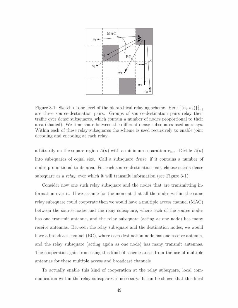
u1

u2

u3

MAC

BC

w1

w2

w3

Figure 3-1: Sketch of one level of the hierarchical relaying scheme. Here (ui, wi)3i=1

are three source-destination pairs. Groups of source-destination pairs relay theirtraffic over dense subsquares, which contain a number of nodes proportional to theirarea (shaded). We time share between the different dense subsquares used as relays.Within each of these relay subsquares the scheme is used recursively to enable jointdecoding and encoding at each relay.

arbitrarily on the square region A(n) with a minimum separation rmin. Divide A(n)

into subsquares of equal size. Call a subsquare dense, if it contains a number of

nodes proportional to its area. For each source-destination pair, choose such a dense

subsquare as a relay, over which it will transmit information (see Figure 3-1).

Consider now one such relay subsquare and the nodes that are transmitting in-

formation over it. If we assume for the moment that all the nodes within the same

relay subsquare could cooperate then we would have a multiple access channel (MAC)

between the source nodes and the relay subsquare, where each of the source nodes

has one transmit antenna, and the relay subsquare (acting as one node) has many

receive antennas. Between the relay subsquare and the destination nodes, we would

have a broadcast channel (BC), where each destination node has one receive antenna,

and the relay subsquare (acting again as one node) has many transmit antennas.

The cooperation gain from using this kind of scheme arises from the use of multiple

antennas for these multiple access and broadcast channels.

To actually enable this kind of cooperation at the relay subsquare, local com-

munication within the relay subsquares is necessary. It can be shown that this local

49

communication problem is actually the same as the original problem, but at a smaller

scale. Hence we can use the same scheme recursively to solve this subproblem. We

terminate the recursion after several iterations, at which point we use simple time

sharing to bootstrap the scheme.

The construction of the hierarchical relaying scheme is presented in detail in Sec-

tion 3.2.1. A back-of-the-envelope calculation of the per-node rate it achieves is

presented in Section 3.2.2. A detailed analysis of the hierarchical relaying scheme is

presented in Sections 3.4 and 3.5.

3.2.1 Construction

Recall that

A(b) , [0,√b]2

is the square region of area b. The scheme described here assumes that n nodes are

placed arbitrarily in A(n) with minimum separation rmin ∈ (0, 1). We want to find

some rate, say ρ0, that can be supported for all n source-destination pairs of a given

permutation traffic matrix λUC(n). The scheme that is described below is “recursive”

(and hence hierarchical) in the following sense. In order to achieve rate ρ0 for n nodes

in A(n), it will use as a building block a scheme for supporting rate ρ1 for a network

of

n1 ,n

2γ(n)

nodes over A(a1) (square of area a1) with

a1 ,n

γ(n)

for any permutation traffic matrix λUC(n1) of n1 nodes. Here the branching factor

γ(n) is a function such that γ(n) → ∞ as n → ∞. We will optimize over the choice

of γ(n) later. The same construction is used for the scheme over A(a1), and so on. In

general, our scheme operates as follows at level ℓ ≥ 0 of the hierarchy (or recursion).

50

In order to achieve rate ρℓ for any permutation traffic matrix λUC(nℓ) over

nℓ ,n

2ℓγℓ(n)

nodes in A(aℓ), with

aℓ ,n

γℓ(n),

use as a building block a scheme achieving rate ρℓ+1 over nℓ+1 nodes in A(aℓ+1) for

any permutation traffic matrix λUC(nℓ+1). The recursion is terminated at some level

L(n) to be chosen later.

We now describe how the hierarchy is constructed between levels ℓ and ℓ + 1 for

0 ≤ ℓ < L(n). Each source-destination pair chooses some subsquare as a relay over

which it transmits its message. This relaying of messages takes place in two phases

— a multiple access phase and a broadcast phase. We first describe the selection of

relay subsquares, then the operation of the network during the multiple access and

broadcast phases, and finally the termination of the hierarchical construction.

Setting up Relays

Given nℓ nodes in A(aℓ), divide the square region A(aℓ) into γ(n) equal sized sub-

squares. Denote them by Ak(aℓ+1)γ(n)k=1 . Call a subsquare dense if it contains at

least nℓ/2γ(n) = nℓ+1 nodes. In other words, a dense subsquare contains a number of

nodes of at least a 1/2ℓ+1 fraction of its area. We show that since the nodes in A(aℓ)

have constant minimum separation rmin, a subsquare can contain at most O(aℓ+1) (i.e.

O(aℓ/γ(n))) nodes, and hence that there are at least Θ(2−ℓγ(n)) dense subsquares.

Each source-destination pair chooses a dense subsquare such that both the source

and the destination are at a distance Ω(√aℓ+1) from it. We call this dense subsquare

the relay of this source-destination pair. We show that the relays can be chosen such

that each relay subsquare has at most nℓ+1 communication pairs that use it as relay,

and we assume this worst case in the following discussion.

51

...

. . .

. . .

...

. . .

. . .

...

. . .

. . .

...

. . .

. . .

...

. . .

. . .

...

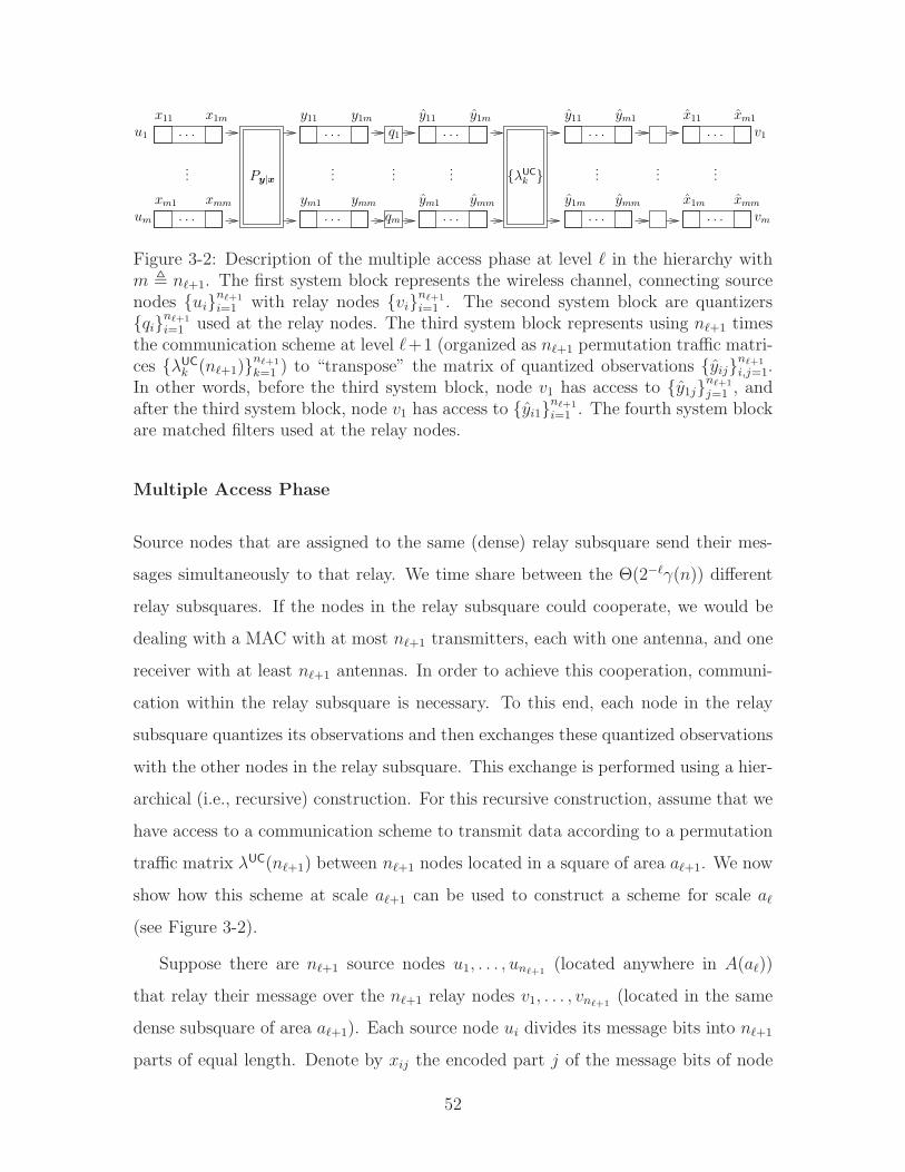
xm1 xmm

x11 x1m y11 y1m

ym1 ymm

y11 y1m

ym1 ymm y1m ymm x1m xmm

vm

v1

xm1x11ym1y11

...Py|x

u1

um qm

q1

λUC

k

Figure 3-2: Description of the multiple access phase at level ℓ in the hierarchy withm , nℓ+1. The first system block represents the wireless channel, connecting sourcenodes uinℓ+1

i=1 with relay nodes vinℓ+1

i=1 . The second system block are quantizersqinℓ+1

i=1 used at the relay nodes. The third system block represents using nℓ+1 timesthe communication scheme at level ℓ+1 (organized as nℓ+1 permutation traffic matri-ces λUC

k (nℓ+1)nℓ+1

k=1 ) to “transpose” the matrix of quantized observations yijnℓ+1

i,j=1.In other words, before the third system block, node v1 has access to y1jnℓ+1

j=1 , andafter the third system block, node v1 has access to yi1nℓ+1

i=1 . The fourth system blockare matched filters used at the relay nodes.

Multiple Access Phase

Source nodes that are assigned to the same (dense) relay subsquare send their mes-

sages simultaneously to that relay. We time share between the Θ(2−ℓγ(n)) different

relay subsquares. If the nodes in the relay subsquare could cooperate, we would be

dealing with a MAC with at most nℓ+1 transmitters, each with one antenna, and one

receiver with at least nℓ+1 antennas. In order to achieve this cooperation, communi-

cation within the relay subsquare is necessary. To this end, each node in the relay

subsquare quantizes its observations and then exchanges these quantized observations

with the other nodes in the relay subsquare. This exchange is performed using a hier-

archical (i.e., recursive) construction. For this recursive construction, assume that we

have access to a communication scheme to transmit data according to a permutation

traffic matrix λUC(nℓ+1) between nℓ+1 nodes located in a square of area aℓ+1. We now

show how this scheme at scale aℓ+1 can be used to construct a scheme for scale aℓ

(see Figure 3-2).

Suppose there are nℓ+1 source nodes u1, . . . , unℓ+1(located anywhere in A(aℓ))

that relay their message over the nℓ+1 relay nodes v1, . . . , vnℓ+1(located in the same

dense subsquare of area aℓ+1). Each source node ui divides its message bits into nℓ+1

parts of equal length. Denote by xij the encoded part j of the message bits of node

52

ui (xij is really a large sequence of channel symbols; to simplify the exposition, we

shall, however, assume it is only a single symbol). The message parts corresponding

to xijnℓ+1

i=1 will be relayed over node vj, as will become clear in the following. Sources

uinℓ+1

i=1 transmit xijnℓ+1

i=1 at time j for j ∈ 1, . . . nℓ+1.

Let ykj be the observed channel output at relay vk at time j. Note that ykj depends

only on channel inputs xijnℓ+1

i=1 . In order to decode the message parts corresponding

to xijnℓ+1

i=1 at relay node vj , it needs to obtain the observations yijnℓ+1

i=1 from all

other relay nodes. In other words, all relays need to exchange information. For this,

each relay vk quantizes its observation ykjnℓ+1

j=1 at an appropriate rate K independent

of n to obtain ykjnℓ+1

j=1 . Quantized observation ykj is to be sent from relay vk to relay

vj . Thus, each of the nℓ+1 relay nodes now has a message of size K for every other

relay node.

This communication demand within the relay subsquare can be organized as nℓ+1

permutation traffic matrices λUCj (nℓ+1)nℓ+1

j=1 between the nℓ+1 relay nodes. Note that

these relay nodes are located in the same square of area aℓ+1. In other words, we are

now faced with the original problem, but at smaller scale aℓ+1. Therefore, using nℓ+1

times the assumed scheme for transmitting according to a permutation traffic matrix

for nℓ+1 nodes inA(aℓ+1), relay vj can obtain all quantized observations yijnℓ+1

i=1 . Now

vj uses nℓ+1 matched filters on yijnℓ+1

i=1 to obtain estimates xijnℓ+1

i=1 of xijnℓ+1

i=1 . In

other words, each node vj computes1

xij =

nℓ+1∑

k=1

h†ui,vk[j]√∑

k|hui,vk[j]|2

ykj

for every i ∈ 1, . . . , nℓ+1. Using these estimates it then decodes the messages

corresponding to xijnℓ+1

i=1 .

1Note that, since we assume full CSI, node vj has access to the channel gains hui,vk[j]i,k at

any time t ≥ j. In particular, this is the case at the time the matched filtering is performed.

53

...

. . .

. . .

......

. . .

. . .

...

. . .

. . .

...

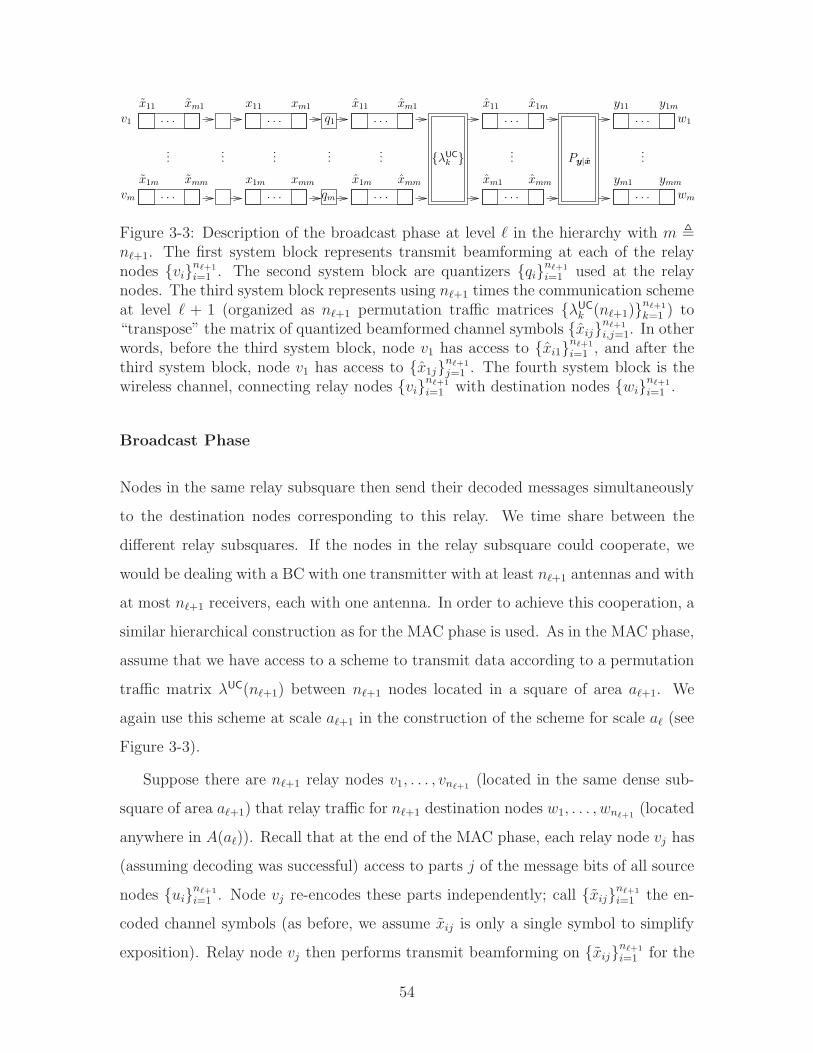
w1

xm1x11

xmmx1mxmm

q1

xm1x11

x1mxmmx1m

x11 xm1

v1

vm qm

. . .

. . .

...

x11 x1m

xmmxm1

...

. . .

. . .

y11 y1m

ymmym1

Py|xλUC

k

wm

Figure 3-3: Description of the broadcast phase at level ℓ in the hierarchy with m ,nℓ+1. The first system block represents transmit beamforming at each of the relaynodes vinℓ+1

i=1 . The second system block are quantizers qinℓ+1

i=1 used at the relaynodes. The third system block represents using nℓ+1 times the communication schemeat level ℓ + 1 (organized as nℓ+1 permutation traffic matrices λUC

k (nℓ+1)nℓ+1

k=1 ) to“transpose” the matrix of quantized beamformed channel symbols xijnℓ+1

i,j=1. In otherwords, before the third system block, node v1 has access to xi1nℓ+1

i=1 , and after thethird system block, node v1 has access to x1jnℓ+1

j=1 . The fourth system block is thewireless channel, connecting relay nodes vinℓ+1

i=1 with destination nodes winℓ+1

i=1 .

Broadcast Phase

Nodes in the same relay subsquare then send their decoded messages simultaneously

to the destination nodes corresponding to this relay. We time share between the

different relay subsquares. If the nodes in the relay subsquare could cooperate, we

would be dealing with a BC with one transmitter with at least nℓ+1 antennas and with

at most nℓ+1 receivers, each with one antenna. In order to achieve this cooperation, a

similar hierarchical construction as for the MAC phase is used. As in the MAC phase,

assume that we have access to a scheme to transmit data according to a permutation

traffic matrix λUC(nℓ+1) between nℓ+1 nodes located in a square of area aℓ+1. We

again use this scheme at scale aℓ+1 in the construction of the scheme for scale aℓ (see

Figure 3-3).

Suppose there are nℓ+1 relay nodes v1, . . . , vnℓ+1(located in the same dense sub-

square of area aℓ+1) that relay traffic for nℓ+1 destination nodes w1, . . . , wnℓ+1(located

anywhere in A(aℓ)). Recall that at the end of the MAC phase, each relay node vj has

(assuming decoding was successful) access to parts j of the message bits of all source

nodes uinℓ+1

i=1 . Node vj re-encodes these parts independently; call xijnℓ+1

i=1 the en-

coded channel symbols (as before, we assume xij is only a single symbol to simplify

exposition). Relay node vj then performs transmit beamforming on xijnℓ+1

i=1 for the

54

nℓ+1 transmit antennas of vknℓ+1

k=1 to be sent at time T + j (for some appropriately

chosen T > 0 not depending on j). Call xkj the resulting channel symbol to be sent

from relay node vk. Then2

xkj =∑

i

h†vk ,wi[T + j]√∑

k|hvk,wi[T + j]|2

xij .

In order to actually send this channel symbol, relay node vk needs to obtain xkj from

node vj. Thus, again all relay nodes need to exchange information.

To enable local cooperation within the relay subsquare, each relay node vj quan-

tizes its beamformed channel symbols xkjnℓ+1

k=1 at an appropriate rate K log(n) with

K independent of n to obtain xkjnℓ+1

k=1 . Now, quantized value xkj is sent from relay

vj to relay vk. Thus, each of the nℓ+1 relay nodes now has a message of size K log(n)

for every other relay node.

This communication demand within the relay subsquare can be organized as nℓ+1

permutation traffic matrices λUC

k (nℓ+1)nℓ+1

k=1 between the nℓ+1 relay nodes. Note

that these relay nodes are located in the same square of area aℓ+1. Hence, we are

again faced with the original problem, but at smaller scale aℓ+1. Using nℓ+1 times

the assumed scheme for transmitting according to a permutation traffic matrix for

nℓ+1 nodes in A(aℓ+1), relay vk can obtain all quantized beamformed channel symbols

xkjnℓ+1

j=1 . Now each vk sends xkj over the wireless channel at time instance T + j

(with T chosen to account for the preceding MAC phase and the local cooperation in

the BC phase). Call yij the received channel output at destination node wi at time

instance T + j. Using yij , destination node wi can now decode part j of the message

bits of its source node ui.

Spatial Re-Use and Termination of Recursion

The scheme performs appropriately weighted time division multiplexing among dif-

ferent levels 0 ≤ ℓ ≤ L(n). Within any level ℓ ≥ 1, multiple regions of the original

2Note that, since we only assume causal CSI, relay node vj does not actually have access tohvk,wi

[T + j]k,i at the time the beamforming is performed. This problem can, however, be cir-cumvented. The details are provided in the proofs (see Lemma 3.10).

55

square A(n) of area n are being operated in parallel. The details related to the effects

of interference between different regions operating at the same level of hierarchy are

discussed in the proofs.

The recursive construction terminates at some large enough level L = L(n) (to be

chosen later). At this scale, we have nL nodes in area A(aL). A permutation traffic

matrix at this level comprises nL source-destination pairs. These transmissions are

performed using simple time sharing. Again, multiple regions in the original square

of area n at level L are active simultaneously.

3.2.2 Achievable Rates

Here we present a back-of-the-envelope calculation of the per-node rate ρHR(n) achiev-

able with the hierarchical relaying scheme described in the previous section. The

complete proof is stated in Section 3.5. We assume throughout that long block codes

and corresponding optimal decoders are used for transmission.

Instead of computing the rate achieved by hierarchical relaying, it will be conve-

nient to instead analyze its inverse, i.e., the time utilized for transmission of a single

message bit from each source to its destination under a permutation traffic matrix

λUC(n). Using the hierarchical relaying scheme, each message travels through L lev-

els of the hierarchy. Call τℓ(n) the amount of time spent for the transmission of one

message bit between each of the nℓ source-destination pairs at level ℓ in the hierarchy.

We compute τℓ(n) recursively.

At any level ℓ ≥ 1, there are multiple regions of area aℓ operating at the same

time. Due to the spatial re-use, each of these regions gets to transmit a constant

fraction of time. It can be shown that the addition of interference due to this spatial

re-use leads only to a constant loss in achievable rate. Hence the time required to send

one message bit is only a constant factor higher than the one needed if region A(aℓ)

is considered separately. Consider now one such region A(aℓ). By the time-sharing

construction, only one of its Θ(2−ℓγ(n)) dense relay subsquares of area aℓ+1 is active

at any given moment. Hence the time required to operate all relay subsquares is a

Θ(2−ℓγ(n)) factor higher than for just one relay subsquare separately. Consider now

56

one such relay subsquare, and assume nℓ+1 source nodes in A(aℓ) communicate each

nℓ+1 message bits to their respective destination nodes through a MAC phase and

BC phase with the help of the nℓ+1 relay nodes in this relay subsquare of area aℓ+1.

In the MAC phase, each of the nℓ+1 sources simultaneously sends one bit to each

of the nℓ+1 relay nodes. The total time for this transmission is composed of two terms.

i) Transmission of nℓ+1 message bits from each of the nℓ+1 source nodes to equally

many relay nodes. Since we time share between Θ(2−ℓγ(n)) relay subsquares,

we can transmit with an average power constraint of Θ(2−ℓγ(n)) during the

time a relay subsquare is active, and still satisfies the overall average power

constraint of 1. With this “bursty” transmission strategy, we require a total of

O

(nℓ+1

aα/2ℓ

2−ℓγ(n)nℓ+1

)= O

(nℓ+14

ℓγℓ(1−α/2)(n)nα/2−1)

(3.1)

channel uses to transmit nℓ+1 bits per source node. The terms on the left-

hand side of (3.1) can be understood as follows: nℓ+1 is the number of bits to

be transmitted; aα/2ℓ is the power loss since most nodes communicate over a

distance of Θ(a1/2ℓ ); 2−ℓγ(n) is the average transmit power; nℓ+1 is the multiple-

antenna gain, since we have that many transmit and receive antennas.

ii) We show that constant rate quantization of the received observations at the

relays is sufficient. Hence the nℓ+1 bits for all sources generate O(nℓ+1) trans-

missions at level ℓ+ 1 of the hierarchy. Therefore,

O(nℓ+1τℓ+1(n)) (3.2)

channel uses are needed to communicate all quantized observations to their

respective relay nodes.

Combining (3.1) and (3.2), accounting for the factor 2−ℓγ(n) loss due to time division

between relay subsquares, we obtain that the transmission time for one message bit

57

from each source to the relay subsquare in the MAC phase at level ℓ is

τMAC

ℓ (n) = O(2ℓγ1+ℓ(1−α/2)(n)nα/2−1 + τℓ+1(n)

). (3.3)

Next, we compute the number of channel uses per message bit received by the

destination nodes in the BC phase. Similar to the MAC phase, each of the nℓ+1

relay nodes has nℓ+1 message bits out of which one bit is to be transmitted to each

of the nℓ+1 destination nodes. Since there are nℓ+1 relay nodes, each destination

node receives nℓ+1 message bits. As before the required transmission time has two

components.

i) Transmission of the encoded and quantized message bits from each of the nℓ+1

relay nodes to all other relay nodes at level ℓ + 1 of the hierarchy. We show

that each message bit results in O((ℓ + 1) logn

)quantized bits. Therefore,

O(nℓ+1(ℓ + 1) logn

)bits need to be transmitted from each relay node. This

requires

O(nℓ+1(ℓ+ 1) log(n)τℓ+1(n)

)(3.4)

channel uses.

ii) Transmission of nℓ+1 message bits from the relay nodes to each destination

node. As before, we use bursty transmission with an average power constraint

of Θ(2−ℓγ(n)) during the fraction Θ(2ℓγ−1(n)) of time each relay subsquare is

active (this satisfies the overall average power constraint of 1). Using this bursty

strategy requires

O

(nℓ+1

aα/2ℓ

2−ℓγ(n)nℓ+1

)= O

(nℓ+14

ℓγℓ(1−α/2)(n)nα/2−1)

(3.5)

channel uses for transmission of nℓ+1 bits per destination node. As in the MAC

phase, nℓ+1 in the left hand side of (3.5) can be understood as the number

of bits to be transmitted, aα/2ℓ as the power loss for communicating over dis-

tance Θ(a1/2ℓ ), 2−ℓγ(n) as the average transmit power, and nℓ+1 as the multiple-

58

antenna gain.

Combining (3.4) and (3.5), accounting for a factor 2−ℓγ(n) loss due to time division

between relay subsquares, the transmission time for one message bit from the relays

to each destination node in the BC phase at level ℓ is

τBC

ℓ (n) = O(2ℓγ1+ℓ(1−α/2)(n)nα/2−1 + (ℓ+ 1) log(n)τℓ+1(n)

). (3.6)

From (3.3) and (3.6), we obtain the following recursion

τℓ(n) = τMAC

ℓ (n) + τBC

ℓ (n)

= O(2ℓγ1+ℓ(1−α/2)(n)nα/2−1 + (ℓ+ 1) log(n)τℓ+1(n)

)

= O(2Lγ(n)nα/2−1 + L log(n)τℓ+1(n)

), (3.7)

where we have used α > 2. This recursion holds for all 0 ≤ ℓ < L. At level L, we time

share among nL nodes in region A(aL) with a permutation traffic matrix λUC(nL).

Each of the nL source-destination pairs uses the wireless channel for 1/nL fraction of

the time at power O(nL), satisfying the average power constraint. This achieves a

rate of at least Ω(a−α/2L ) between any source-destination pair. Equivalently

τL(n) = O(aα/2L )

= O(nα/2γ−Lα/2(n)

)

= O(nα/2γ−L(n)

). (3.8)

Using the recursion (3.7) L times and combining with (3.8), we have

τ0(n) = O(nα/2−12Lγ(n) + L log(n)τ1(n)

)

= . . .

= O(nα/2−1

(L log(n)

)L2Lγ(n) +

(L log(n)

)LτL(n)

)

= O(nα/2−1

(L log(n)

)L(2Lγ(n) + nγ−L(n)

)). (3.9)

59

The term(L log(n)

)L(2Lγ(n) + nγ−L(n)

)(3.10)

is the “loss” factor over the desired order nα/2−1 scaling, and we now choose the

branching factor γ(n) and the hierarchy depth L , L(n) to make it small. Fix a

δ ∈ (0, 1/2) and set3

L(n) , log1/2−δ(n),

γ(n) , n1/(L(n)+1).

With this

(L(n) log(n)

)L(n) ≤ n2 log−1/2−δ(n) log log(n),

2L(n)γ(n) ≤ nlog−1/2−δ(n)+logδ−1/2(n),

nγ−L(n)(n) ≤ nlogδ−1/2(n).

Since δ > 0, the nlogδ−1/2(n) term dominates in (3.9), and we obtain

τ0(n) ≤ b(n)nα/2−1,

where

b(n) ≤ nO(logδ−1/2(n)).

Hence the per-node rate of the hierarchical relaying scheme is lower bounded as

ρHR(n) = 1/τ0(n) ≥ b(n)n1−α/2,

with

b(n) ≥ n−O(logδ−1/2(n)).

3There are several choices of L(n) and γ(n) that result in the “loss” factor (3.10) to be of orderno(1). The choice here is convenient for the slow fading case discussed in detail in Chapter 3.5.2.However, other choices are possible as well.

60

Note that to minimize the loss term, we should choose δ > 0 to be small.

3.3 Cooperative Multi-Hop Scheme

In this section, we provide a brief description of the cooperative multi-hop scheme.

The details of the construction and the analysis of its performance can be found in

Section 3.8.

Recall that a node placement V (n) is µ-regular at resolution d(n) if every square

[id(n), (i + 1)d(n)] × [jd(n), (j + 1)d(n)] for some i, j ∈ N contains at least µd2(n)

nodes. Given such a node placement V (n), divide it into squares of sidelength d(n).

Consider four adjacent squares, combined into a bigger square of sidelength 2d(n).

By the regularity assumption on V (n), this bigger square contains at least 4µd2(n)

nodes. Hence we can apply the hierarchical relaying scheme introduced in Section 3.2

to support any permutation traffic within this bigger square at a per-node rate of

b(n)(d2(n))1−α/2 = b(n)d2−α(n),

where b(n) is essentially of order n− log−1/2(n). By properly choosing the permutation

traffic matrices within every possible such bigger square of sidelength 2d(n) and with

appropriate spatial re-use, nodes in each square of sidelength d(n) can communicate

with neighboring squares at a sum rate of

d2(n)b(n)d2−α(n) = b(n)d4−α(n).

We now construct a graph with n/d2(n) vertices, each corresponding to one square

of sidelength dn in A(n). Nodes corresponding to neighboring squares are connected

by an edge with edge capacity

b(n)d4−α(n).

The resulting graph is depicted in Figure 3-4. Note that with the above communica-

tion procedure if messages can be routed over this graph then the same messages can

61

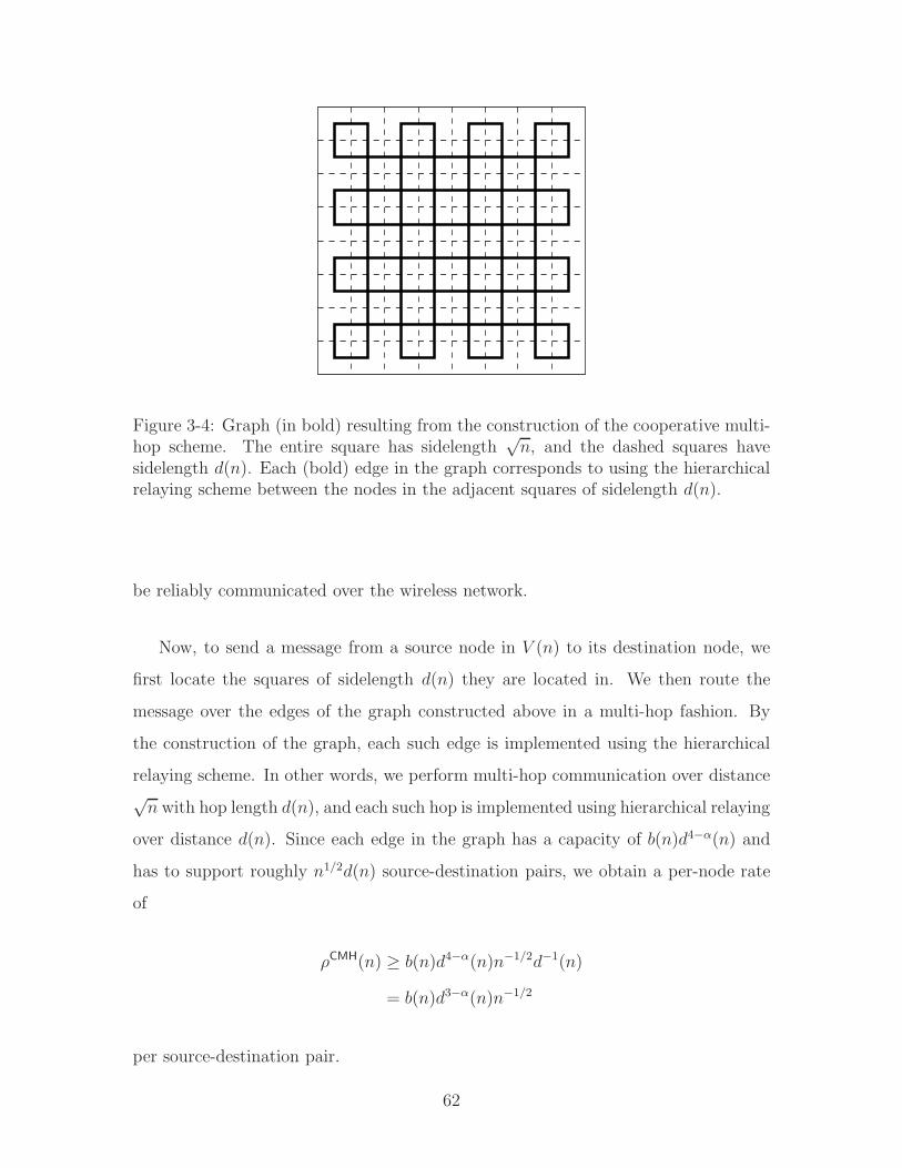
Figure 3-4: Graph (in bold) resulting from the construction of the cooperative multi-hop scheme. The entire square has sidelength

√n, and the dashed squares have

sidelength d(n). Each (bold) edge in the graph corresponds to using the hierarchicalrelaying scheme between the nodes in the adjacent squares of sidelength d(n).

be reliably communicated over the wireless network.

Now, to send a message from a source node in V (n) to its destination node, we

first locate the squares of sidelength d(n) they are located in. We then route the

message over the edges of the graph constructed above in a multi-hop fashion. By

the construction of the graph, each such edge is implemented using the hierarchical

relaying scheme. In other words, we perform multi-hop communication over distance√n with hop length d(n), and each such hop is implemented using hierarchical relaying

over distance d(n). Since each edge in the graph has a capacity of b(n)d4−α(n) and

has to support roughly n1/2d(n) source-destination pairs, we obtain a per-node rate

of

ρCMH(n) ≥ b(n)d4−α(n)n−1/2d−1(n)

= b(n)d3−α(n)n−1/2

per source-destination pair.

62

3.4 Analysis of the Hierarchical Relaying Scheme

In this section, we analyze in detail the hierarchical relaying scheme. Throughout

Sections 3.4.1 to 3.4.3, we consider communication at level ℓ, 0 ≤ ℓ < L = L(n), of

the hierarchy. All constants Ki are independent of ℓ.

Recall that at level ℓ in the hierarchy, we have a square region A(aℓ) of area

aℓ ,n

γℓ(n)

containing (at least)

nℓ ,n

2ℓγℓ(n)

nodes V (nℓ). We divide A(aℓ) into γ(n) subsquares of area aℓ+1. Recall that a

subsquare of area aℓ+1 in level ℓ of the hierarchy is called dense if it contains at least

nℓ+1 nodes. We impose a power constraint of Pℓ(n) = Θ(2−ℓγ(n)) during the time any

particular relay subsquare is active. Since we time share between Θ(2−ℓγ(n)) relay

subsquares, this satisfies the overall average power constraint (by choosing constants

appropriately).

Since other regions of area aℓ are active at the same time as the one under con-

sideration, we have to deal with interference. To this end, we consider a slightly

more general noise model that includes the experienced interference at the relay sub-

squares. More precisely, we assume that, for all u ∈ V (nℓ), the additive noise term

zu[t]t is independent of the signal xu[t]t and of the channel gains hu,v[t]v,t; that

the noise term is stationary and ergodic across time t, but with arbitrary dependence

across nodes u; and that the noise has zero mean and bounded power N0 independent

of n. Note that we do not require the additive noise term to be Gaussian. In the

above, N0 accounts for both noise (which has power 1 in the original model) as well

as interference. We show in Section 3.5 that these assumptions are valid.

63

Recall the following choice of γ(n) and L(n):

L(n) , log1/2−δ(n),

γ(n) , n1/(L(n)+1),(3.11)

with δ ∈ (0, 1/2) independent of n. This choice satisfies

γ(n) ≤ γ(n) if n ≤ n,

γL(n)(n) ≤ n for all n,

2−L(n)γ(n) → ∞ as n→ ∞,

(3.12)

The first condition in (3.12) implies that the number of subsquares γ(n) we divide

A(n) into increases in n. The second condition implies that the subsquare area aL(n)

at the last level of the hierarchy is bigger than 1. As we shall see, the third condition

implies that the number of dense subsquares at the last level of the hierarchy (and

hence at every level) grows unbounded as n→ ∞ (see Lemma 3.6 below).

Throughout Section 3.4, we consider the fast fading channel model. Slow fading

is discussed in Section 3.5.2.

3.4.1 Setting up Relays

The first lemma states that the minimum-separation requirement rmin ∈ (0, 1) implies

that a constant fraction of subsquares must be dense. We point out that this is the

only consequence of the minimum-separation requirement used to prove Theorem 3.1.

Thus Theorem 3.1 remains valid if we just assume that Lemma 3.6 below holds

directly. See also Section 3.10.4 for further details.

Lemma 3.6. For any V (nℓ) ⊂ A(aℓ) with |V (nℓ)| ≥ nℓ and with minimum separation

rmin ∈ (0, 1), each of its subsquares of area aℓ+1 contains at most K1aℓ/γ(n) nodes,

and there are at least K22−ℓγ(n) dense subsquares, for some constants K1 and K2.

Proof. Put a circle of radius rmin/2 around each node. By the minimum-separation

requirement, these circles do not intersect. Each node covers an area of πr2min/4.

64

Increasing the sidelength of each subsquare by rmin, this provides a total area of

(√aℓ/γ(n) + rmin

)2 ≤ aℓ

γ(n)(1 + rmin)

2

in which the circles around these nodes are packed. Here we have used that γℓ+1(n) ≤n by (3.12), and therefore

γ(n) ≤ n/γℓ(n) = aℓ.

Hence there can be at most K1aℓ/γ(n) nodes per subsquare with

K1 , 4(1 + rmin)

2

πr2min

.

Note that, since rmin < 1, we have K1 > 1.

Let d(nℓ) be the number of dense subsquares in A(aℓ), and therefore γ(n)−d(nℓ) is

the number of subsquares that are not dense. By the argument in the last paragraph,

each dense subsquare contains at most K1aℓ/γ(n) nodes, and those subsquares that

are not dense contain less than nℓ+1 nodes by the definition of dense subsquares.

Hence d(nℓ) must satisfy

d(nℓ)K1aℓ/γ(n) +(γ(n) − d(nℓ)

)nℓ+1 ≥ |V (nℓ)| ≥ nℓ.

Thus, using aℓ = 2ℓnℓ, nℓ+1 = nℓ/2γ(n), we have

d(nℓ)K12ℓ + (γ(n) − d(nℓ))/2 ≥ γ(n).

As K1 > 1, this yields

d(nℓ) ≥1 − 1/2

K12ℓ − 1/2γ(n) ≥ 2−ℓ

2K1γ(n) = K22

−ℓγ(n),

with

K2 ,1

2K1

.

65

Consider V (nℓ) ⊂ A(aℓ) with |V (nℓ)| ≥ nℓ, and choose arbitrary K22−ℓγ(n)

dense subsquares of area aℓ+1 (as guaranteed by Lemma 3.6). Call those subsquares

Ak(aℓ+1)K22−ℓγ(n)k=1 . For each source-destination pair, we now select one such dense

subsquare to relay traffic over. To avoid bottlenecks, this selection has to be done

such that all relay subsquares carry approximately the same amount of traffic. More-

over, for technical reasons, the distances from the source and the destination to the

relay subsquare cannot be too small.

Formally, the selection of relay subsquares can be described by the schedules S ∈0, 1nℓ×K22−ℓγ(n) with su,k = 1 if source node u relays traffic over dense subsquare

k, and S ∈ 0, 1K22−ℓγ(n)×nℓ with sk,w = 1 if destination node w receives traffic

from dense subsquare k. With slight abuse of notation, let ru,Ak(aℓ+1) be the distance

between node u ∈ V (nℓ) and the closest point in Ak(aℓ+1), i.e.,

ru,Ak(aℓ+1) , minv∈Ak(aℓ+1)

ru,v. (3.13)

Define the sets

S(nℓ) ,S ∈ 0, 1nℓ×K22−ℓγ(n) :0 ≤∑nℓ

u=1 su,k ≤ nℓ+1 ∀k,

0 ≤∑K22−ℓγ(n)k=1 su,k ≤ 1 ∀u,

su,k = 1 implies ru,Ak(aℓ+1) ≥√

2aℓ+1 ∀u, k

(3.14)

and

S(nℓ) ,S ∈ 0, 1K22−ℓγ(n)×nℓ : ST ∈ S(nℓ)

.

The sets S(nℓ) and S(nℓ) are the collection of schedules satisfying the conditions

mentioned in the last paragraph. More precisely, the first condition in (3.14) ensures

that at most nℓ+1 source-destination pairs relay over the same dense subsquare, the

second condition ensures that each source-destination pair chooses at most one relay

subsquare, and the third condition ensures that sources and destinations are at least

at distance√

2aℓ+1 from the chosen relay subsquare.

Next, we prove that any node placement that satisfies Lemma 3.6 allows for a de-

66

composition of any permutation traffic matrix λUC(nℓ) into a small number of sched-

ules belonging to S(nℓ) and S(nℓ).

Lemma 3.7. There exists K3 such that for all n large enough (independent of ℓ),

and every permutation traffic matrix λUC(nℓ) ∈ 0, 1nℓ×nℓ we can find K32ℓ schedules

S(i)(nℓ)K32ℓ

i=1 ⊂ S(nℓ), S(i)(nℓ)K32ℓ

i=1 ⊂ S(nℓ) satisfying

λUC(nℓ) =

K32ℓ∑

i=1

S(i)(nℓ)S(i)(nℓ),

for some constant K3.

Proof. Pick an arbitrary source-destination pair in λUC(nℓ), and consider the sub-

squares containing the source and the destination node. Since each subsquare has

side length√aℓ+1, there are at most 50 subsquares at distance less than

√2aℓ+1 from

either of those two subsquares. As 2−L(n)γ(n) → ∞ as n→ ∞ by (3.12), there exists

K (independent of ℓ) such that for n ≥ K we have 50 ≤ K22−ℓ−1γ(n). Since there

are at least K22−ℓγ(n) dense subsquares by Lemma 3.6, there must exist at least

K22−ℓ−1γ(n) dense subsquares that are at distance at least

√2aℓ+1 from both the

subsquares containing the source and the destination node.

In order to construct a decomposition of λUC(nℓ), we use the following procedure.

Sequentially, each of the nℓ source-destination pairs chooses one of the (at least)

K22−ℓ−1γ(n) dense subsquares at distance at least

√2aℓ+1 that has not already been

chosen by nℓ+1 other pairs. If any source-destination pair cannot select such a sub-

square, then stop the procedure and use the source-destination pairs matched with

dense subsquares so far to define matrices S(1)(nℓ) and S(1)(nℓ). Now, remove all the

matched source-destination pairs, forget that dense subsquares were matched to any

source-destination pair and repeat the above procedure, going through the remaining

source-destination pairs.

Let

K3 , 4/K2.

We claim that by repeating this process of generating matrices S(i)(nℓ) and S(i)(nℓ),

67

we can match all source-destination pairs to some dense subsquare with at most

K32ℓ such matrices. Indeed, a new pair of matrices is generated only when a source-

destination pair cannot be matched to any of its available (at least) K22−ℓ−1γ(n)

dense subsquares. If this happens, all these dense subsquares are matched by nℓ+1 =

nℓ/2γ(n) pairs. Hence at least K22−ℓ−2nℓ source-destination pairs are matched in

each “round”. Since there are nℓ total pairs, we need at most

nℓ

K22−ℓ−2nℓ= K32

ℓ

matrices S(i)(nℓ) and S(i)(nℓ).

For a permutation traffic matrix λUC(nℓ), communication proceeds as follows.

Write

λUC(nℓ) =

K32ℓ∑

i=1

S(i)(nℓ)S(i)(nℓ)

as in Lemma 3.7. Split time into K32ℓ equal length time slots. In slot i, we use

S(i)(nℓ)S(i)(nℓ) as our traffic matrix. Consider without loss of generality i = 1 in the

following. Write

S(1)(nℓ)S(1)(nℓ) =

K22−ℓγ(n)∑

k=1

S(1,k)(nℓ+1)S(1,k)(nℓ+1),

where S(1,k)(nℓ+1)S(1,k)(nℓ+1) is the traffic relayed over the dense subsquare Ak(aℓ+1).

We time share between the schedules for k ∈ 1, . . . , K22−ℓγ(n). Consider now any

such k. In the worst case, there are exactly nℓ+1 communication pairs to be relayed

over Ak(aℓ+1), and the relay subsquare Ak(aℓ+1) contains exactly nℓ+1 nodes. We

shall assume this worst case in the following.

We focus on transmission according to the traffic matrix S(1,1)(nℓ+1)S(1,1)(nℓ+1).

Let V (nℓ+1) be the nodes in A1(aℓ+1), and let U(nℓ+1) and W (nℓ+1) be the source and

destination nodes of S(1,1)(nℓ+1)S(1,1)(nℓ+1), respectively. In other words, the source

nodes U(nℓ+1) communicate to their respective destination nodes W (nℓ+1) using the

nodes V (nℓ+1) as relays.

68

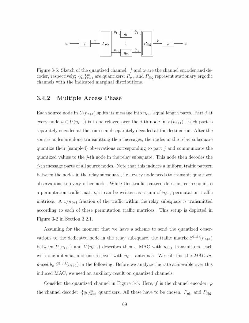
w fx

Py|x

... w

y1

ymqm

q1y1

ym

xPx|y ϕ

Figure 3-5: Sketch of the quantized channel. f and ϕ are the channel encoder and de-coder, respectively; qkm

k=1 are quantizers; Py|x and Px|y represent stationary ergodicchannels with the indicated marginal distributions.

3.4.2 Multiple Access Phase

Each source node in U(nℓ+1) splits its message into nℓ+1 equal length parts. Part j at

every node u ∈ U(nℓ+1) is to be relayed over the j-th node in V (nℓ+1). Each part is

separately encoded at the source and separately decoded at the destination. After the

source nodes are done transmitting their messages, the nodes in the relay subsquare

quantize their (sampled) observations corresponding to part j and communicate the

quantized values to the j-th node in the relay subsquare. This node then decodes the

j-th message parts of all source nodes. Note that this induces a uniform traffic pattern

between the nodes in the relay subsquare, i.e., every node needs to transmit quantized

observations to every other node. While this traffic pattern does not correspond to

a permutation traffic matrix, it can be written as a sum of nℓ+1 permutation traffic

matrices. A 1/nℓ+1 fraction of the traffic within the relay subsquare is transmitted

according to each of these permutation traffic matrices. This setup is depicted in

Figure 3-2 in Section 3.2.1.

Assuming for the moment that we have a scheme to send the quantized obser-

vations to the dedicated node in the relay subsquare, the traffic matrix S(1,1)(nℓ+1)

between U(nℓ+1) and V (nℓ+1) describes then a MAC with nℓ+1 transmitters, each

with one antenna, and one receiver with nℓ+1 antennas. We call this the MAC in-

duced by S(1,1)(nℓ+1) in the following. Before we analyze the rate achievable over this

induced MAC, we need an auxiliary result on quantized channels.

Consider the quantized channel in Figure 3-5. Here, f is the channel encoder, ϕ

the channel decoder, qkmk=1 quantizers. All these have to be chosen. Py|x and Px|y,

69

on the other hand, represent fixed stationary ergodic channels with the indicated

marginal distributions. We call R the rate of the channel code (f, ϕ) and Rkmk=1

the rates of quantizers qkmk=1.

Lemma 3.8. If there exist distributions Px and Pyk|ykm

k=1 such that R < I(x; x)

and Rk > I(yk; yk), ∀k, then(R, Rkm

k=1

)is achievable over the quantized channel.

Proof. The proof follows from a simple extension of Theorem 1 in Appendix II of [38].

Lemma 3.9. Let the additive noise zvv∈V (nℓ+1) be uncorrelated (over v). For the

MAC induced by S(1,1)(nℓ+1) with per-node average power constraint Pℓ(n) ≤ n−1ℓ+1a

α/2ℓ ,

a rate of

ρMAC

ℓ (n) ≥ K4Pℓ(n)nℓ+1a−α/2ℓ

per source node is achievable, and the number of bits required at each relay node to

quantize the observations is at most K5 bits per nℓ+1 total message bits4 sent by the

source nodes, for some constants K4 and K5.

Proof. The source nodes send signals with a power of (essentially) n−1ℓ+1a

α/2ℓ for a

fraction Pℓ(n)nℓ+1a−α/2ℓ ≤ 1 of time and are silent for the remaining time. To ensure

that interference is uniform, the time slots during which the nodes send signals are

chosen randomly as follows. Generate independently for each region A(aℓ) a Bernoulli

process B[t]t∈N with parameter Pℓ(n)nℓ+1a−α/2ℓ /(1 + η) ≤ 1 for some small η > 0.

The nodes in A(aℓ) are active whenever B[t] = 1 and remain silent otherwise. Since

the blocklength of the codes used is assumed to be large, this satisfies the average

power constraint of Pℓ(n) with high probability for any η > 0. Since we are interested

only in the scaling of capacity, we ignore the additional 1/(1+η) term in the following

to simplify notation. Clearly, we only need to consider the fraction of time during

which B[t] = 1.

Let y be the received vector at the relay subsquare, y the (componentwise) quan-

4Total message bits refers to the sum of all message bits transmitted by the nℓ+1 source nodes.

70

tized observations. We use a matched filter at the relay subsquare, i.e.,

xu =h†

u

‖hu‖y,

where column vector hu = hu,vv∈V (nℓ+1) are the channel gains between node u ∈U(nℓ+1) and the nodes in the relay subsquare V (nℓ+1). The use of a matched filter is

possible since we assume full CSI is available at all the nodes.

We now use Lemma 3.8 to show that we can design quantizers qvv∈V (nℓ+1) of con-

stant rate and achieve a per-node communication rate of at least K4Pℓ(n)nℓ+1a−α/2ℓ .

The first channel in Lemma 3.8 (see Figure 3-5) will correspond to the wireless chan-

nel between a source node u and its relay subsquare V (nℓ+1). The second “channel”

in Lemma 3.8 will correspond to the matched filter used at the relay subsquare. To

apply Lemma 3.8, we need to find a distribution for xu and for yv|yv. Define

ru , ru,A1(aℓ+1)/√

2aℓ ≤ 1

with ru,A1(aℓ+1) as in (3.13), to be the normalized distance of the source node u ∈U(nℓ+1) to the relay subsquare A1(aℓ+1). For each u ∈ U(nℓ+1), let

xu ∼ NC(0, rαun

−1ℓ+1a

α/2ℓ )

independent of xu for u 6= u, and let yv = yv + zv for zv ∼ NC(0,∆2) independent of

y and for some ∆2 > 0. Note that the channel input xu has power that depends on

the normalized distance ru (i.e., only nodes u ∈ U(nℓ+1) that are at maximal distance√

2aℓ from the relay subsquare transmit at full available power). This is to ensure

that all signals are received at roughly the same strength by the relays.

We proceed by computing I(yv; yv|hu,v) and I(xu; xu|hu,v) as required in

Lemma 3.8 (the conditioning on hu,v being due to the availability of full CSI).

Note first that by construction of S(1,1)(nℓ+1) (see (3.14)), we have for u ∈ U(nℓ+1)

and v ∈ V (nℓ+1)

ru,A1(aℓ+1) ≤ ru,v ≤ 2ru,A1(aℓ+1),

71

and hence1

2√

2aℓ

≤ ru

ru,v

≤ 1√2aℓ

. (3.15)

From this, and since |hu,v|2 = r−αu,v , we obtain

2−3α/2a−α/2ℓ ≤ |hu,v|2rα

u ≤ 2−α/2a−α/2ℓ ,

2−3α/2nℓ+1a−α/2ℓ ≤ ‖hu‖2rα

u ≤ 2−α/2nℓ+1a−α/2ℓ .

(3.16)

We start by computing I(yv; yv|hu,v). We have

yv =∑

u∈U(nℓ+1)

hu,vxu + zv + zv,

and hence yv has mean zero and variance

E(|yv|2) =∑

u∈U(nℓ+1)

|hu,v|2rαun

−1ℓ+1a

α/2ℓ +N0 + ∆2

≤ nℓ+12−α/2a

−α/2ℓ n−1

ℓ+1aα/2ℓ +N0 + ∆2

= 2−α/2 +N0 + ∆2,

where we have used (3.16). Hence

I(yv; yv|hu,v) = h(yv|hu,v) − h(yv|yv, hu,v)

≤ log(2πeE(|yv|2)

)− log(2πe∆2)

≤ log(2πe(2−α/2 +N0 + ∆2)

)− log(2πe∆2)

= log(1 +

2−α/2 +N0

∆2

). (3.17)

We now compute I(xu; xu|hu,v). We have

xu = ‖hu‖xu +∑

u∈U(nℓ+1)\u

h†uhu

‖hu‖xu +

h†u

‖hu‖(z + z).

72

Conditioned on huu∈U(nℓ+1),

‖hu‖xu ∼ NC

(0, ‖hu‖2rα

un−1ℓ+1a

α/2ℓ

),

and

E

(∣∣∣∑

u∈U(nℓ+1)\uh†

uhu

‖hu‖xu +

h†u

‖hu‖(z + z)

∣∣∣2∣∣∣hu

)

= n−1ℓ+1a

α/2ℓ

∑

u∈U(nℓ+1)\urαu

|h†uhu|2

‖hu‖2+N0 + ∆2,

where we have used the assumption that zvv∈V (nℓ+1) are uncorrelated. Using (3.16),

this is, in turn, upper bounded by

23α/2rαun

−2ℓ+1a

αℓ

∑

u∈U(nℓ+1)\urαu |h†

uhu|2 +N0 + ∆2.

Similarly, we can lower bound the received signal power as

E(‖hu‖2|xu|2

)≥ 2−3α/2.

Since Gaussian noise is the worst additive noise under a power constraint [18], and

applying Jensen’s inequality to the convex function log(1 + 1/x), we obtain

I(xu; xu|hu,v)

≥ E

(log

(1 +

2−3α/2

23α/2rαun

−2ℓ+1a

αℓ

∑u∈U(nℓ+1)\u r

αu |h†

uhu|2 +N0 + ∆2

))

≥ log

(1 +

2−3α/2

23α/2rαun

−2ℓ+1a

αℓ

∑u∈U(nℓ+1)\u r

αuE(|h†

uhu|2)

+N0 + ∆2

). (3.18)

We have for u 6= u,

E(|h†

uhu|2)

= E(h†uhuh

†uhu)

73

=∑

v∈V (nℓ+1)

|hu,v|2|hu,v|2

=∑

v∈V (nℓ+1)

r−αu,vr

−αu,v , (3.19)

and hence using (3.15)

E

(rαu

∑

u∈U(nℓ+1)\urαu |h†

uhu|2)

=∑

u∈U(nℓ+1)\u

∑

v∈V (nℓ+1)

rαur

−αu,v r

αur

−αu,v

≤ 2−αn2ℓ+1a

−αℓ .

Therefore we can continue (3.18) as

I(xu; xu|hu,v) ≥ log

(1 +

2−3α/2

2α/2 +N0 + ∆2

), K4. (3.20)

Using (3.17) and (3.20) in Lemma 3.8, and observing that we only communicate

during a fraction

Pℓ(n)nℓ+1a−α/2ℓ ≤ 1

of time yields a per source node rate ρMAC

ℓ (n) arbitrarily close to

K4Pℓ(n)nℓ+1a−α/2ℓ

and a quantizer of rate arbitrarily close to

log(1 +

2−α/2 +N0

∆2

)

bits per observation at each relay node. Since by (3.20) the mutual information

I(xu; xu|hu,v) is at least K4 for every u ∈ U(nℓ+1) during the fraction of time we

actually communicate, this implies that there are at most 1/K4 observations at each

relay node per nℓ+1 total message bits. Thus the number of bits per relay node

74

required to quantize the observations is at most

K5 ,1

K4log(1 +

2−α/2 +N0

∆2

)

bits per nℓ+1 total message bits sent by the source nodes.

3.4.3 Broadcast Phase

At the end of the MAC phase, each node in the relay subsquare received a part of the

message sent by each source node. In the BC phase, each node in the relay subsquare

encodes these messages together for nℓ+1 transmit antennas. The encoded message

is then quantized and communicated to all the nodes in the relay subsquare. These

nodes then send the quantized encoded message to the destination nodes W (nℓ+1).

Note that this again induces a uniform traffic pattern between the nodes in the

relay subsquare, i.e., every node needs to transmit quantized encoded messages to

every other node. While this traffic pattern does not correspond to a permutation

traffic matrix it can be written as a sum of nℓ+1 permutation traffic matrices. A

1/nℓ+1 fraction of the traffic within the relay subsquare is transmitted according to

each of these permutation traffic matrices. This setup is depicted in Figure 3-3 in

Section 3.2.1.

Assuming for the moment that we have a scheme to send the quantized en-

coded messages to the corresponding nodes in the relay subsquare, the traffic matrix

S(1,1)(nℓ+1) between V (nℓ+1) and W (nℓ+1) describes then a BC with one transmitter

with nℓ+1 antennas and nℓ+1 receivers, each with one antenna. We call this the BC

induced by S(1,1)(nℓ+1) in the following.

Lemma 3.10. For the BC induced by S(1,1)(nℓ+1) with per-node average power con-

straint Pℓ(n) ≤ n−1ℓ+1a

α/2ℓ , a rate of

ρBC

ℓ (n) ≥ K6Pℓ(n)nℓ+1a−α/2ℓ

is achievable per destination node, and the number of bits required to quantize the

75

observations is at most K7(ℓ+1) log(n) bits at each relay node per nℓ+1 total message

bits5 received by the destination nodes, for some constants K6 and K7.

Proof. Consider a node v ∈ V (nℓ+1) in the relay subsquare, say the first one. From

the MAC phase, this node received the first part of the messages of each source

node u ∈ U(nℓ+1). We would like to jointly encode these message parts at the relay

node using transmit beamforming, and then transmit the corresponding encoded

signal using all the nodes in the relay subsquare. However, this cannot be done

directly because at the encoding time, the future channel state at transmission time

is unknown.

We circumvent this problem by reordering the signals to be transmitted at the

relay nodes as follows. Let

θv,wv∈V (nℓ+1),w∈W (nℓ+1) ∈ 0, π/2, π, 3π/2n2ℓ+1.

be a “quantized” channel state. The part of the messages at node v in the relay

subsquare is encoded for nℓ+1 transmit nodes with an assumed channel gain of

hv,w[t] = r−α/2v,w exp(

√−1θv,w[t]),

where the θv,w[t]v,w,t are cycled as a function of t through all possible values in

0, π/2, π, 3π/2n2ℓ+1. The components of the encoded messages are then quantized

and each component sent to the corresponding node in the relay subsquare. Once all

nodes in the relay subsquare have received the encoded message, they send in each

time slot a sample of the encoded messages corresponding to the quantized channel

state closest (in Euclidean distance) to the actual channel realization in that time

slot. By ergodicity of θu,v[t]t, each quantized channel state is used approximately

the same number of times. More precisely, as the message length grows to infinity,

we can send samples of the encoded message parts a 1/(1 + η) fraction of time with

probability approaching 1 for any η > 0. Since we have no constraint on the encoding

5Total message bits refers to the sum of all message bits received by the nℓ+1 destination nodes.

76

delay in our setup, we can choose η arbitrarily small, and given that we are only

interested in scaling laws, we will ignore this term in the following to simplify notation.

Note that the destination nodes can reorder the received samples since we assume full

CSI. In the following, we let θv,wv,w be the random quantized channel state induced

by θv,wv,w through the above procedure. Denote by hv,wv,w the corresponding

channel gains.

As in the MAC phase, the nodes in the relay subsquare send signals at a power

(essentially) n−1ℓ+1a

α/2ℓ a fraction Pℓ(n)nℓ+1a

−α/2ℓ ≤ 1 of time and are silent for the

remaining time. To create interference at uniform power, this is done in the same

randomized manner as in the MAC phase. Generate independently for each region

A(aℓ) a Bernoulli process B[t]t∈N with parameter Pℓ(n)nℓ+1a−α/2ℓ /(1 + η) for some

small η > 0. The nodes in A(aℓ) are active whenever B[t] = 1 and remain silent

otherwise. As before, we ignore the additional 1/(1 + η) term. Again we only need

to consider the fraction of time during which B[t] = 1.

Consider the message part at a relay node for destination node w ∈ W (nℓ+1).

We encode this part independently; call xw the encoded message part. The relay

node then performs transmit beamforming to construct the encoded message for all

its destination nodes, i.e.,

x =∑

w∈W (nℓ+1)

h†w

‖hw‖xw,

where row vector hw = hv,wv∈V (nℓ+1) contains the channel gains to node w, and

where we have used |hv,w| = |hv,w|. The relay node then quantizes the vector of

encoded messages componentwise and forwards the quantized version x to the other

nodes in the relay subsquare. These nodes then send x over the channel to the

destination nodes. The received signal at destination node w is thus

yw = hwx + zw.

With this, we have the setup considered in Lemma 3.8 (with different variable

names). The first “channel” in Lemma 3.8 (see Figure 3-5) will correspond to the

77

transmit beamforming used at the relay subsquare. The second channel in Lemma 3.8

will now correspond to the wireless channel between the relay subsquare V (nℓ+1) and

a destination node w. To apply Lemma 3.8, we need to find a distribution for xw and

for xv|xv. We also need to guarantee that xv satisfies the power constraint at each

node v in the relay subsquare. For each w ∈W (nℓ+1), let

xw ∼ NC(0, Kn−1ℓ+1a

α/2ℓ )

(for some K to be chosen later) independent of xw for w 6= w, and let xv = xv + zv

for zv ∼ NC(0,∆2) independent of x and for some ∆2 > 0. We then have

yw =hwh†

w

‖hw‖xw +

∑

w∈W (nℓ+1)\w

hwh†w

‖hw‖xw + hwz + zw.

We proceed by computing I(xv; xv|hu,v) and I(xw; yw|hu,v) as required in

Lemma 3.8 (the conditioning on hu,v is again due to availability of full CSI). Note

first that by construction of S(1,1)(nℓ+1), we have for any w ∈W (nℓ+1)

2 minv∈V (nℓ+1)

rv,w ≥ maxv∈V (nℓ+1)

rv,w,

and therefore|hv,w|2‖hw‖2

≤(minv∈V (nℓ+1) rv,w

)−α

nℓ+1

(maxv∈V (nℓ+1) rv,w

)−α ≤ 2α

nℓ+1. (3.21)

We start by computing I(xv; xv|hu,v). xv has mean zero and variance

E(|xv|2

)=

∑

w∈W (nℓ+1)

|hv,w|2‖hw‖2

Kn−1ℓ+1a

α/2ℓ + ∆2

≤ nℓ+12α

nℓ+1Kn−1

ℓ+1aα/2ℓ + ∆2

≤ n−1ℓ+1a

α/2ℓ , (3.22)

for

K , 2−α(1 − ∆2),

78

which is positive for ∆2 < 1, and where we have used (3.21) and that

n−1ℓ+1a

α/2ℓ ≥ 2ℓ+1γ(n) ≥ 1

by (3.12). Equation (3.22) shows that xv satisfies the power constraint of node v in

the relay subsquare V (nℓ+1). Moreover, we obtain

I(xv; xv|hu,v) = h(xv|hu,v) − h(xv|xv, hu,v)

≤ log(2πeE

(|xv|2

))− log(2πe∆2)

≤ log

(n−1

ℓ+1aα/2ℓ

∆2

). (3.23)

It remains to compute I(xw; yw|hu,v). Note that the encoding procedure guar-

antees that

cos(π/4)2‖hw‖4 ≤ |hwh†w|2 ≤ ‖hw‖4.

Moreover, for w 6= w,

E(|hwh

†w|2)

= E(hwh†whwh†

w)

=∑

v∈V (nℓ+1)

E(|hvw|2|hvw|2

)

=∑

v∈V (nℓ+1)

E(|hvw|2|hvw|2

)

= E(|hwh

†w|2).

From this, we get by a similar argument as in Lemma 3.9 that

I(xw; yw|hu,v) ≥ K6. (3.24)

Using (3.23) and (3.24) in Lemma 3.8, and observing that we only communicate

during a fraction

Pℓ(n)nℓ+1a−α/2ℓ

79

of time, yields a per destination node rate ρBC

ℓ (n) arbitrarily close to

K6Pℓ(n)nℓ+1a−α/2ℓ

bits per channel use and a quantizer rate arbitrarily close to

log(n−1

ℓ+1aα/2ℓ

∆2

)

bits per encoded sample. Since by (3.24) mutual information I(xw; yw|hu,v) is at

least K6 for every w ∈W (nℓ+1) during the fraction of time we actually communicate,

this implies that there are at most 1/K6 encoded message samples for each relay

node per nℓ+1 total message bits received by the destination nodes W (nℓ+1). Thus

the number of bits required at each relay node to quantize the encoded message

samples is at most

1

K6

log(n−1

ℓ+1aα/2ℓ

∆2

)=

1

K6

log( 1

∆22ℓ+1γ1+ℓ(1−α/2)(n)nα/2−1

)

≤ 1

K6

log( 1

∆22ℓ+1nα/2

)

≤ K7(ℓ+ 1) log(n)

bits per nℓ+1 total message bits received by the destination nodes, and where we have

used γ(n) ≤ n by (3.12).

3.5 Proof of Theorem 3.1

The proof of Theorem 3.1 is split into two parts. In Section 3.5.1 we prove the theorem

for fast fading, and in Section 3.5.2 for slow fading.

3.5.1 Fast Fading

In this section, we prove Theorem 3.1 under fast fading, i.e., θu,v[t]t is stationary

and ergodic in t. We first prove that the assumptions on the power constraint and

80

the interference made in Section 3.4 (see Lemmas 3.9 and 3.10) during the analysis of

one level of the hierarchical relaying scheme are valid. We then use the results proved

there to analyze the behavior of the entire hierarchy, yielding a lower bound on the

per-node rate achievable with hierarchical relaying.

We first argue that the constraint Pℓ(n) ≤ n−1ℓ+1a

α/2ℓ needed in Lemmas 3.9 and

3.10 is satisfied. Consider the hierarchical relaying scheme as described in Section 3.2,

and fix a level ℓ, 0 ≤ ℓ < L = L(n), in this hierarchy. At level ℓ, we have a square

of area aℓ = n/γℓ(n) with nℓ = n/2ℓγℓ(n) source-destination pairs. Since we are time

sharing between K22−ℓγ(n) relay subsquares at this level, we have an average power

constraint of

Pℓ(n) , K22−ℓγ(n)

during the time any particular relay subsquare is active. Since α > 2 and since

nγ−L(n)(n) → ∞ as n→ ∞, we have, for n large enough (independent of ℓ), that

Pℓ(n) = K22−ℓγ(n)

≤ 2−ℓγ(n)( n

γL(n)(n)

)α/2−1

≤ 2ℓ+1γ(n)( n

γℓ(n)

)α/2−1

= n−1ℓ+1a

α/2ℓ .

Therefore the power constraints in Lemmas 3.9 and 3.10 are satisfied.

We continue by analyzing the interference caused by spatial re-use. Recall that the

MAC and BC phases at level ℓ induce permutation traffic within the dense subsquares

at level ℓ+ 1. The permutation traffic within those dense subsquares at level ℓ+ 1 is

transmitted in parallel with spatial re-use. We now describe in detail how this spatial

re-use is performed. Partition the subsquares of area aℓ+1 (i.e., at level ℓ + 1) into

four subsets such that in each subset all subsquares are at distance at least√aℓ+1

from each other. The traffic that the MAC and BC phases at level ℓ induce in each

of the relay subsquares at level ℓ + 1 is transmitted simultaneously within all relay

subsquares in the same subset. Consider now one such subset. We show that at any

81

relay subsquare the interference from other relay subsquares in the same subset is

stationary and ergodic within each phase, additive (i.e., independent of the signals

and channel gains in this relay subsquare), and of bounded power N0−1 independent

of n.

We first argue that the interference is stationary and ergodic within each phase.

Note first that on any level ℓ + 1 in the hierarchy, all relay subsquares are either

simultaneously in the MAC phase or simultaneously in the BC phase. Furthermore,

all relay subsquares are also synchronized for transmissions within each of these phases

(recall that the induced traffic in level ℓ + 1 is uniform and is sent sequentially as

permutation traffic). Hence it suffices to show that the interference generated by

either the MAC or BC induced by some permutation traffic matrix is stationary and

ergodic. Since all codebooks for either of these cases are generated as i.i.d. Gaussian

multiplied by a Bernoulli process, and in the BC phase beamformed for stationary

and ergodic fading, this is indeed the case.

The additivity of the interference follows easily for the MAC phase since code-

books are generated independently of the channel realization in this case. Moreover,

since the channel gains are independent from each other and all codebooks are gener-

ated as independent zero mean processes, the interference in the MAC phase is also

uncorrelated (over space) within each relay subsquare. For the BC phase, the code-

book depends only on the channel gains within each relay subsquare at level ℓ + 1.

Since the channel gains within relay subsquares are independent of the channel gains

between relay subsquares, this interference is additive as well.

We now bound the interference power. Note that by the randomized time-sharing

construction within the MAC and BC phases (see Lemmas 3.9 and 3.10), in each

relay subsquare at most nℓ+1 nodes transmit at an average power of 1. In the MAC

phase, all nodes use independently generated codebooks with power at most 1, and

thus the received interference power from another relay subsquare at distance i√aℓ+1

is at most

nℓ+1i−αa

−α/2ℓ+1 = i−α2−(ℓ+1)

( n

γℓ+1(n)

)1−α/2

≤ i−α,

82

by (3.12). In the BC phase, the nodes in each active relay subsquare use beamforming

to transmit to nodes within their own subsquare. Since the channel gains within a

relay subsquare are independent of the channel gains between relay subsquares, the

same calculation as in (3.19) shows that we can upper bound the received interference

power from another relay subsquare at distance i√aℓ+1 by

nℓ+1i−αa

−α/2ℓ+1 ≤ i−α,

in the BC phase as well.

Now, by the way in which we perform spatial re-use, every active relay subsquare

has at most 8i active relay subsquares at distance at least i√aℓ+1. Hence the total

interference power received at an active relay subsquare is at most

∞∑

i=1

8i2αi−α , N0 − 1 <∞

since α > 2. With this, we have shown that the interference term has the properties

required in Lemmas 3.9 and 3.10.

We now apply those two lemmas to obtain a lower bound on the rate achievable

with hierarchical relaying. Call τℓ(n) the number of channel uses to transmit one

bit from each of nℓ source nodes to the corresponding destination nodes at level ℓ.

Lemma 3.7 states that for n large enough (independent of ℓ), we relay over each

dense subsquare at most K32ℓ times. Combining this with Lemma 3.9, we see that

to transmit one bit from each source to its destination at this level we need at most

4K32ℓK22

−ℓγ(n)1

K4Pℓ(n)n−1

ℓ+1aα/2ℓ =

K322ℓ+3

K4

nα/2−1γ1+ℓ(1−α/2)(n)

channel uses for the MAC phase. Here, the factor 4 accounts for the spatial re-use,

K32ℓ accounts for relaying over the same relay subsquares multiple times, K22

−ℓγ(n)

accounts for time sharing between the relay subsquares, and the last term accounts for

the time required to communicate over the MAC. Similarly, combining Lemmas 3.7

83

and 3.10, we need at most

K322ℓ+3

K6nα/2−1γ1+ℓ(1−α/2)(n)

channel uses for the BC phase. Moreover, at level ℓ+ 1 in the hierarchy this induces

a per-node traffic demand of at most K5 bits from the MAC phase, and at most

K7(ℓ+ 1) log(n) from the BC phase. Thus we obtain the following recursion

τℓ(n) ≤ 8K3

( 1

K4+

1

K6

)nα/2−1γ(n)

(4γ1−α/2(n)

)ℓ+ (K5 +K7(ℓ+ 1) log(n))τℓ+1(n)

≤ Knα/2−1γ(n)4ℓ +K(ℓ+ 1) log(n)τℓ+1(n)

≤ Knα/2−1γ(n)4L(n) +KL(n) log(n)τℓ+1(n) (3.25)

for positive constants K, K independent of n and ℓ.

At scale aL, we have nL nodes and source-destination pairs. Time sharing between

all source-destination pairs, we have (during the time we communicate for each node)

an average power constraint of nL. Since at this level we communicate over a distance

of at most 2a1/2L , we have

τL(n) ≤ nL log−1

(1 +

nL

2αN0aα/2L

). (3.26)

Since

nLa−α/2L ≤ nLa

−1L = 2−L(n) → 0

as n→ ∞, we can upper bound (3.26) as

τL(n) ≤ K ′aα/2L

= K ′nα/2γ−L(n)α/2(n)

≤ K ′nα/2γ−L(n)(n) (3.27)

for some constant K ′.

84

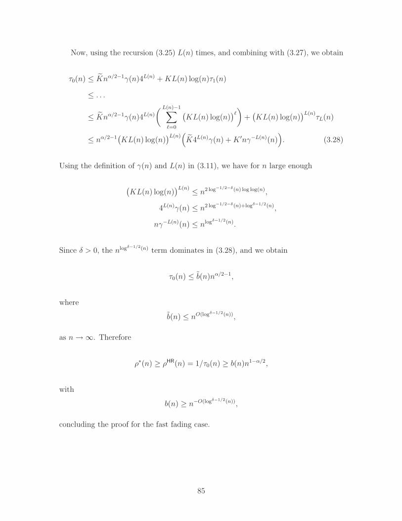
Now, using the recursion (3.25) L(n) times, and combining with (3.27), we obtain

τ0(n) ≤ Knα/2−1γ(n)4L(n) +KL(n) log(n)τ1(n)

≤ . . .

≤ Knα/2−1γ(n)4L(n)

( L(n)−1∑

ℓ=0

(KL(n) log(n)

)ℓ)

+(KL(n) log(n)

)L(n)τL(n)

≤ nα/2−1(KL(n) log(n)

)L(n)(K4L(n)γ(n) +K ′nγ−L(n)(n)

). (3.28)

Using the definition of γ(n) and L(n) in (3.11), we have for n large enough

(KL(n) log(n)

)L(n) ≤ n2 log−1/2−δ(n) log log(n),

4L(n)γ(n) ≤ n2 log−1/2−δ(n)+logδ−1/2(n),

nγ−L(n)(n) ≤ nlogδ−1/2(n).

Since δ > 0, the nlogδ−1/2(n) term dominates in (3.28), and we obtain

τ0(n) ≤ b(n)nα/2−1,

where

b(n) ≤ nO(logδ−1/2(n)),

as n→ ∞. Therefore

ρ∗(n) ≥ ρHR(n) = 1/τ0(n) ≥ b(n)n1−α/2,

with

b(n) ≥ n−O(logδ−1/2(n)),

concluding the proof for the fast fading case.

85

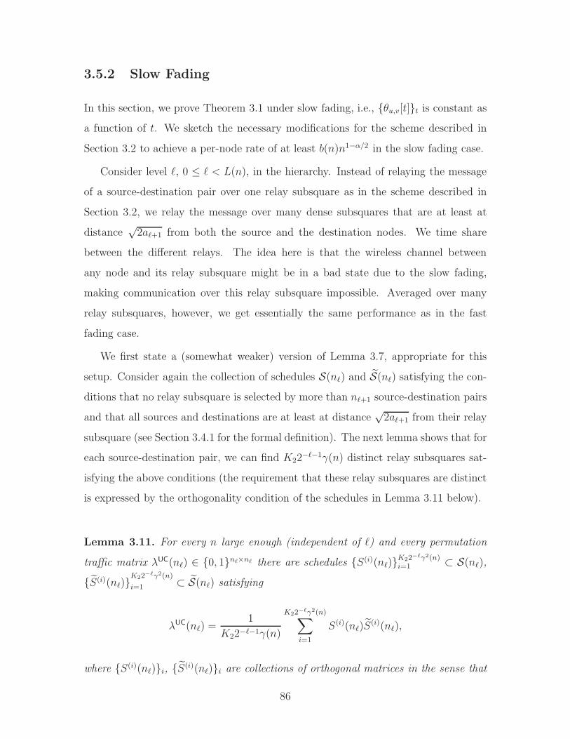
3.5.2 Slow Fading

In this section, we prove Theorem 3.1 under slow fading, i.e., θu,v[t]t is constant as

a function of t. We sketch the necessary modifications for the scheme described in

Section 3.2 to achieve a per-node rate of at least b(n)n1−α/2 in the slow fading case.

Consider level ℓ, 0 ≤ ℓ < L(n), in the hierarchy. Instead of relaying the message

of a source-destination pair over one relay subsquare as in the scheme described in

Section 3.2, we relay the message over many dense subsquares that are at least at

distance√

2aℓ+1 from both the source and the destination nodes. We time share

between the different relays. The idea here is that the wireless channel between

any node and its relay subsquare might be in a bad state due to the slow fading,

making communication over this relay subsquare impossible. Averaged over many

relay subsquares, however, we get essentially the same performance as in the fast

fading case.

We first state a (somewhat weaker) version of Lemma 3.7, appropriate for this

setup. Consider again the collection of schedules S(nℓ) and S(nℓ) satisfying the con-

ditions that no relay subsquare is selected by more than nℓ+1 source-destination pairs

and that all sources and destinations are at least at distance√

2aℓ+1 from their relay

subsquare (see Section 3.4.1 for the formal definition). The next lemma shows that for

each source-destination pair, we can find K22−ℓ−1γ(n) distinct relay subsquares sat-

isfying the above conditions (the requirement that these relay subsquares are distinct

is expressed by the orthogonality condition of the schedules in Lemma 3.11 below).

Lemma 3.11. For every n large enough (independent of ℓ) and every permutation

traffic matrix λUC(nℓ) ∈ 0, 1nℓ×nℓ there are schedules S(i)(nℓ)K22−ℓγ2(n)i=1 ⊂ S(nℓ),

S(i)(nℓ)K22−ℓγ2(n)

i=1 ⊂ S(nℓ) satisfying

λUC(nℓ) =1

K22−ℓ−1γ(n)

K22−ℓγ2(n)∑

i=1

S(i)(nℓ)S(i)(nℓ),

where S(i)(nℓ)i, S(i)(nℓ)i are collections of orthogonal matrices in the sense that

86

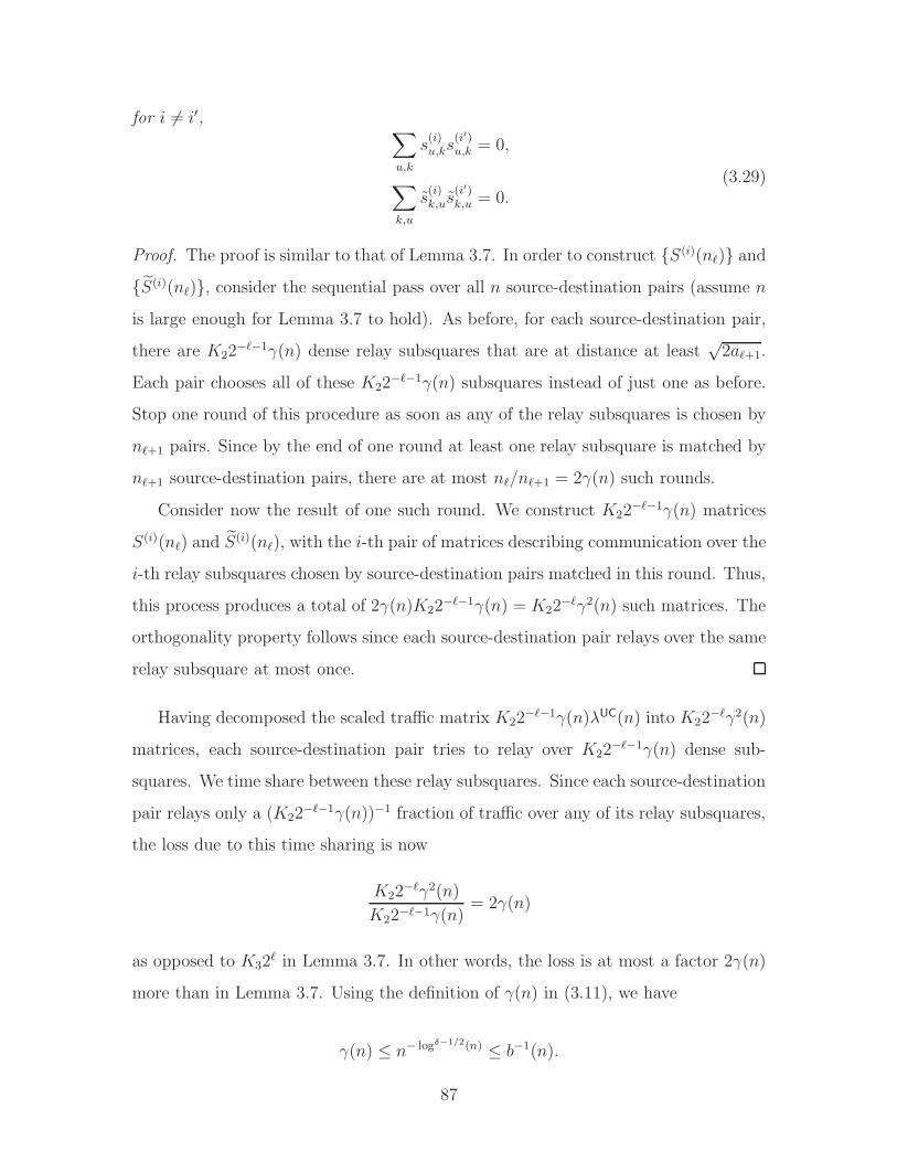
for i 6= i′, ∑

u,k

s(i)u,ks

(i′)u,k = 0,

∑

k,u

s(i)k,us

(i′)k,u = 0.

(3.29)

Proof. The proof is similar to that of Lemma 3.7. In order to construct S(i)(nℓ) and

S(i)(nℓ), consider the sequential pass over all n source-destination pairs (assume n

is large enough for Lemma 3.7 to hold). As before, for each source-destination pair,

there are K22−ℓ−1γ(n) dense relay subsquares that are at distance at least

√2aℓ+1.

Each pair chooses all of these K22−ℓ−1γ(n) subsquares instead of just one as before.

Stop one round of this procedure as soon as any of the relay subsquares is chosen by

nℓ+1 pairs. Since by the end of one round at least one relay subsquare is matched by

nℓ+1 source-destination pairs, there are at most nℓ/nℓ+1 = 2γ(n) such rounds.

Consider now the result of one such round. We construct K22−ℓ−1γ(n) matrices

S(i)(nℓ) and S(i)(nℓ), with the i-th pair of matrices describing communication over the

i-th relay subsquares chosen by source-destination pairs matched in this round. Thus,

this process produces a total of 2γ(n)K22−ℓ−1γ(n) = K22

−ℓγ2(n) such matrices. The

orthogonality property follows since each source-destination pair relays over the same

relay subsquare at most once.

Having decomposed the scaled traffic matrix K22−ℓ−1γ(n)λUC(n) into K22

−ℓγ2(n)

matrices, each source-destination pair tries to relay over K22−ℓ−1γ(n) dense sub-

squares. We time share between these relay subsquares. Since each source-destination

pair relays only a (K22−ℓ−1γ(n))−1 fraction of traffic over any of its relay subsquares,

the loss due to this time sharing is now

K22−ℓγ2(n)

K22−ℓ−1γ(n)= 2γ(n)

as opposed to K32ℓ in Lemma 3.7. In other words, the loss is at most a factor 2γ(n)

more than in Lemma 3.7. Using the definition of γ(n) in (3.11), we have

γ(n) ≤ n− logδ−1/2(n) ≤ b−1(n).

87

In other words, this additional loss is small.

Consider now a specific relay subsquare. If a source-destination pair can commu-

nicate over this relay subsquare at a rate at least 1/64-th of the rate achievable in the

fast fading case (given by Lemmas 3.9 and 3.10), it sends information over this relay.

Otherwise it stays silent during the period of time it is assigned this relay. We now

show that, with probability 1 − o(1) as n → ∞, for every source-destination pair on

every level of the hierarchy at least one quarter of its relay subsquares can support

this rate. As we only communicate over a quarter of the relay subsquares, this implies

that we can achieve at least 1/256-th of the per-node rate for the fast fading case (see

Section 3.5.1), i.e., that b(n)n1−α/2 is achievable with probability 1− o(1) as n→ ∞.

Assume we have for each source-destination pair (u, w) picked K22−ℓ−1γ(n) dense

subsquares over which it can relay; call those relay subsquares Au,w,kK22−ℓ−1γ(n)k=1 .

Consider the event Bu,w,k that source node u can communicate at the desired rate

to destination node w over relay subsquares Au,w,k (assuming, as before, that we can

solve the communication problem within this subsquare).

Let B(i)u,w,k4

i=1 be the events that the interference due to matched filtering in the

MAC phase, the interference from spatial re-use in the MAC phase, the interference

due to beamforming in the BC phase, and the interference from spatial re-use in the

BC phase, are less than 8 times the one for fast fading, respectively. From the proof

of Lemmas 3.9, 3.10, and of Theorem 3.1 for the fast fading case in Section3.5.1, we

see that4⋂

i=1

B(i)u,w,k ⊂ Bu,w,k.

Due to spatial re-use, multiple relay subsquares will be active in parallel. Let H

denote the set of channel gains between active relay subsquares. Using essentially the

same arguments as for the fast fading case (see Lemmas 3.9, 3.10, and Section 3.5.1)

and from Markov’s inequality, we have P(B(i)u,w,k|H) ≥ 7/8 for all i ∈ 1, . . . , 4 and

hence P(Bu,w,k|H) ≥ 1/2.

88

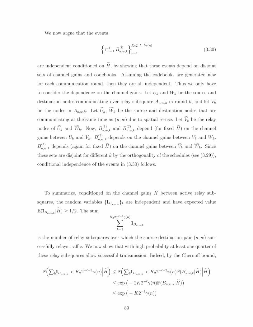
We now argue that the events

∩4

i=1 B(i)u,w,k

K22−ℓ−1γ(n)

k=1(3.30)

are independent conditioned on H, by showing that these events depend on disjoint

sets of channel gains and codebooks. Assuming the codebooks are generated new

for each communication round, then they are all independent. Thus we only have

to consider the dependence on the channel gains. Let Uk and Wk be the source and

destination nodes communicating over relay subsquare Au,w,k in round k, and let Vk

be the nodes in Au,w,k. Let Uk, Wk be the source and destination nodes that are

communicating at the same time as (u, w) due to spatial re-use. Let Vk be the relay

nodes of Uk and Wk. Now, B(1)u,w,k and B

(2)u,w,k depend (for fixed H) on the channel

gains between Uk and Vk. B(3)u,w,k depends on the channel gains between Vk and Wk.

B(4)u,w,k depends (again for fixed H) on the channel gains between Vk and Wk. Since

these sets are disjoint for different k by the orthogonality of the schedules (see (3.29)),

conditional independence of the events in (3.30) follows.

To summarize, conditioned on the channel gains H between active relay sub-

squares, the random variables 11Bu,w,kk are independent and have expected value

E(11Bu,w,k|H) ≥ 1/2. The sum

K22−ℓ−1γ(n)∑

k=1

11Bu,w,k

is the number of relay subsquares over which the source-destination pair (u, w) suc-

cessfully relays traffic. We now show that with high probability at least one quarter of

these relay subsquares allow successful transmission. Indeed, by the Chernoff bound,

P

(∑k11Bu,w,k

< K22−ℓ−3γ(n)

∣∣∣H)≤ P

(∑k11Bu,w,k

< K22−ℓ−2γ(n)P(Bu,w,k|H)

∣∣∣H)

≤ exp(− 2K2−ℓγ(n)P(Bu,w,k|H)

)

≤ exp(−K2−ℓγ(n)

)

89

for some constant K > 0. Since the right-hand side is the same for all H , this implies

P

(∑k11Bu,w,k

< K22−ℓ−3γ(n)

)≤ exp

(−K2−ℓγ(n)

).

In each of the L(n) levels of the hierarchy there are at most n2 source-destination

pairs, and hence by the union bound with probability at least

1 − L(n)n2 exp(−K2−L(n)γ(n)

),

for every source-destination pair on every level of the hierarchy at least one quarter

of its relay subsquares can support the desired rate. By the choices of γ(n) and L(n)

in (3.11), this probability is at least

1 − L(n)n2 exp(−K2−L(n)γ(n)

)≥ 1 − n3 exp

(−K2−L(n)2log(n)/2L(n)

)

≥ 1 − exp(K2log log(n) −K2

12

log1/2+δ(n)−log1/2−δ(n))

≥ 1 − exp(− 2Ω(log1/2+δ(n))

)

≥ 1 − o(1)

as n→ ∞, and for some constant K. This proves that the same order rate as in the

fast fading case can be achieved with high probability for all levels 0 ≤ ℓ < L(n).

It remains to argue that the same holds for level ℓ = L(n). Note that since we

assume phase fading only, the received signal power is only a function of distance and

not of the fading realization. Since at level L(n) we use simple time sharing, this

implies that we can always achieve the same rate at level L(n) as in the fast fading

case.

Hence with probability 1−o(1) as n→ ∞, we achieve the same order rate at each

level 0 ≤ ℓ ≤ L(n) as for fast fading, proving Theorem 3.1 for the slow fading case.

90

3.6 Proof of Theorem 3.2

Here, we provide a generalization and sharpening of the converse in [38]. Most of the

arguments follow [38, Theorem 5.2]. We start by proving a lemma upper bounding

the MIMO capacity.

Consider two subsets S1, S2 ⊂ V (n) such that S1 ∩ S2 = ∅. Assume we allow

the nodes within S1 and S2 to cooperate without any restriction. The maximum

achievable sum rate between the nodes in S1 and S2 is given by the MIMO capacity

C(S1, S2) between them. The next lemma upper bounds C(S1, S2) in terms of the

node distances between the two sets and the normalized channel gains

hu,v ,hu,v√∑v∈S2

r−αu,v

. (3.31)

Lemma 3.12. Under either fast or slow fading, for every α > 2, for any node

placement V (n), and any S1, S2 ⊂ V (n) with S1 ∩ S2 = ∅, we have

C(S1, S2) ≤ 4

(max

1,max

v∈S2

∑

u∈S1

|hu,v|2)∑

u∈S1

∑

v∈S2

r−αu,v .

Proof. Let

H , hu,vu∈S1,v∈S2 ,

H , hu,vu∈S1,v∈S2 ,

be the matrix of (normalized) channel gains between the nodes in S1 and S2. Consider

first fast fading. Under this assumption, we have

C(S1, S2) , maxQ(H)≥0:

E(qu,u)≤1 ∀u∈S1

E

(log det

(I + H†Q(H)H

)).

Define

PS1,S2 ,∑

u∈S1

∑

v∈S2

r−αu,v

91

as the total received power in S2 from S1, and set

Pu,S2 , Pu,S2

with slight abuse of notation. Then

C(S1, S2) = maxQ(H)≥0:

E(qu,u)≤Pu,S2∀u∈S1

E

(log det

(I + H†Q(H)H

))

≤ maxQ(H)≥0:

E(trQ(H))≤PS1,S2

E

(log det

(I + H†Q(H)H

)). (3.32)

Define the event

B ,‖H‖2 > b

for some b and where ‖H‖ denotes the largest singular value of H . In words, B is

the event that the channel gains between S1 and S2 are “good”. We argue that, for

appropriately chosen b, the event B has probability zero (i.e., the channel cannot be

too “good”). By Markov’s inequality

P(B) ≤ b−mE(‖H‖2m), (3.33)

for any m. We continue by upper bounding E(‖H‖2m). We have

‖H‖2k ≤ tr((HH†)k

)

for any k, and hence

E(‖H‖2m) ≤ E

((tr((HH†)k

))m/k). (3.34)

Now, for any k ≥ m, we have by Jensen’s inequality

E

((tr((HH†)k

))m/k)≤(Etr((HH†)k

))m/k

. (3.35)

92

Combining (3.33), (3.34), and (3.35) yields

P(B) ≤ b−m(

Etr((HH†)k

))m/k

(3.36)

for any k ≥ m.

Now, the arguments in [38, Lemma 5.3] show that

E(tr((HH†)k

))≤ tkn

(max

1,max

v∈S2

∑

u∈S1

|hu,v|2)k

,

where tk is the k-th Catalan number. Combining with (3.36), this yields

P(B) ≤(b−1t

1/kk n1/k

(max

1,max

v∈S2

∑

u∈S1

|hu,v|2))m

.

Taking the limit as k → ∞ and using that t1/kk → 4 yields

P(B) ≤(b−14

(max

1,max

v∈S2

∑

u∈S1

|hu,v|2))m

.

Assume

b > 4

(max

1,max

v∈S2

∑

u∈S1

|hu,v|2)

, (3.37)

then taking the limit as m→ ∞ shows that

P(B) = 0.

Using this, we can upper bound (3.32) as

C(S1, S2) ≤ maxQ(H)≥0:

E(trQ(H))≤PS1,S2

E

(tr(H†Q(H)H

))

= maxQ(H)≥0:

E(trQ(H))≤PS1,S2

E

(11Bctr

(H†Q(H)H

))

≤ maxQ(H)≥0:

E(trQ(H))≤PS1,S2

E

(11Bc‖H‖2trQ(H)

)

93

≤ bPS1,S2.

Since this is true for all b satisfying (3.37), we obtain the lemma for the fast fading

case.

Under slow fading

C(S1, S2) , maxQ≥0:

qu,u≤P ∀u∈S1

log det(I + H†QH

),

and the lemma can be obtained by the same steps.

We now proceed to the proof of Theorem 3.2. Consider a vertical cut dividing the

network into two parts. By the minimum-separation requirement, an area of size o(n)

can contain at most o(n) nodes, and hence we can find a cut such that each part is

of size Θ(n) and contains Θ(n) nodes. Call the left part of the cut S. Since there are

Θ(n) nodes in S and in Sc, there are Θ(n) sources in S with their destination in Sc

with probability 1 − o(1). For technical reasons we add a node inside each square in

V (n) of the form [id, (i+ 1)d]× [jd, (j + 1)d] for some i, j ∈ N, where d ,√

2 log(n).

These additional nodes have no traffic demands on their own, and simply help with

the transmission. This can clearly only increase achievable rates. Moreover, this

increases the number of nodes in V by less than a factor 2. We now show that

C(S, Sc) = O(log6(n)n2−α/2

), (3.38)

and hence by the cut-set bound [9, Theorem 14.10.1], and since there are Θ(n) sources

in S with their destination in Sc, we have

ρ∗(n) = O(log6(n)n1−α/2

).

We prove (3.38) using Lemma 3.12. To this end, we need to upper bound

maxv∈Sc

∑

u∈S

|hu,v|2.

94

The proof of [38, Lemma 5.3] shows that if

1. there are less than log(n) nodes inside [i, i + 1] × [j, j + 1] for any i, j ∈0, . . . ,√n− 1,

2. there is at least one node inside [id, (i+ 1)d] × [jd, (j + 1)d] for any i, j, where

d ,√

2 logn,

then

maxv∈Sc

∑

u∈S

|hu,v|2 ≤ K log3(n), (3.39)

and for α ∈ (2, 3]∑

u∈S

∑

v∈Sc

r−αu,v ≤ K log3(n)n2−α/2, (3.40)

for constants K, K. For arbitrary node placement with minimum separation, the first

requirement is satisfied for n large enough, since only a constant number of nodes

can be contained in each area of constant size. By our addition of nodes into V (n)

described above, the second condition is also satisfied. Using Lemma 3.12 with (3.39)

and (3.40) yields (3.38), concluding the proof of Theorem 3.2.

3.7 Proof of Theorem 3.3

Consider a node placement with n/2 nodes located uniformly on [0,√n/4] × [0,

√n]

and n/2 nodes located on [√n/2,

√n]× [0,

√n] with minimum separation rmin = 1/2.

A random traffic matrix λUC(n) is such that at least n/4 communication pairs have

their sources in the left cluster and destinations in the right cluster with probability

1 − o(1). Assume we are dealing with such a λUC(n) in the following.

In this setup, with multi-hop at least one hop has to cross the gap between the

left and the right cluster. Thus, even without any interference from other nodes, we

can obtain at most

ρMH(n) ≤ 4αn−α/2.

Moreover, considering a cut between the two clusters (say, S and Sc), and applying

95

Lemma 3.12 yields that

ρ∗(n) ≤ 16n−1

(max

1,max

v∈Sc

∑

u∈S

|hu,v|2)∑

u∈S

∑

v∈Sc

r−αu,v . (3.41)

Now note that for any u ∈ S, v ∈ Sc, we have

1

4

√n ≤ ru,v ≤ 2

√n.

Hence∑

u∈S

|hu,v|2 =∑

u∈S

r−αu,v∑

v∈Sc r−αu,v

≤ 23α,

and∑

u∈S

∑

v∈Sc

r−αu,v ≤ 4α−1n2−α/2.

Combining this with (3.41) yields

ρ∗(n) ≤ 22+5αn1−α/2

for all α > 2.

3.8 Proof of Theorem 3.4

We construct a cooperative multi-hop communication scheme and lower bound the

per-node rate ρCMH(n) it achieves. We use the hierarchical relaying scheme as build-

ing block. Assume the node placement V (n) is µ-regular at resolution d(n) for all

n ≥ 1. We show that this implies that we can achieve a per-node rate of at least

d3−α(n)n−1/2−β(n) as n→ ∞. Taking the smallest such d(n) then yields the result.

We consider three cases for the value of d(n) (namely, d(n) = Θ(√n), d(n) ≥ no(1),

and d(n) ≤ no(1)). First, if d(n) = Θ(√n) as n → ∞ then the result follows directly

from Theorem 3.1. Considering a subsequence if necessary, we can therefore assume

without loss of generality that d(n) = o(√n) in the following.

96

Second, consider d(n) satisfying

d(n) ≥ n1

2+αlogδ−1/2(n). (3.42)

Divide A(n) into squares of sidelength d(n). Since d(n) = o(√n), the number of

such squares grows unbounded as n → ∞. We now show that we can use multi-

hop communication with a hop length of d(n) where each hops is implemented by

squares cooperatively sending information to a neighboring square. In other words, we

perform cooperative communication at local scale d(n) and multi-hop communication

at global scale√n.

Since V (n) is µ-regular at resolution d(n), each such square contains at least

µd2(n) nodes. Pick the top left most square and construct the square of sidelength

2d(n) consisting of it together with its 3 neighbors. Continue in the same fashion,

partitioning all of A(n) into squares of sidelength 2d(n). Note that each such bigger

square contains at least 4µd2(n) nodes, and we assume this worst case in the following.

Partition A(n) into 4 subsets of those bigger squares such that within each such subset

each square is at distance at least 2d(n) from any other square (see Figure 3-6). We

time share between those 4 subsets. Consider in the following one such subset. For

every bigger square, we construct two permutation traffic matrices λUC1 (4µd2(n)) and

λUC2 (4µd2(n)). In λUC

1 the nodes in the top two squares have as destinations the

nodes in the bottom two squares and the nodes in the bottom two squares have as

destinations the nodes in the top two squares (see Figure 3-6). Similarly, λUC2 contains

communication pairs between left and right squares. We time share between λUC1 and

λUC2 .

Communication according to λUCi within bigger squares in the same subset occurs

simultaneously. We are going to use hierarchical relaying within each bigger square.

This is possible since each such square contains at least 4µd2(n) nodes. We have to

show that the additional interference from bigger squares in the same subset is such

that Theorem 3.1 still applies. In particular, we need to show that the interference

has bounded power, say K. Using the same arguments as in the proof of Theorem 3.1

97

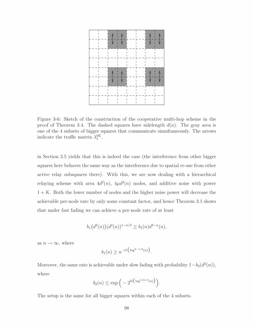
Figure 3-6: Sketch of the construction of the cooperative multi-hop scheme in theproof of Theorem 3.4. The dashed squares have sidelength d(n). The gray area isone of the 4 subsets of bigger squares that communicate simultaneously. The arrowsindicate the traffic matrix λUC

1 .

in Section 3.5 yields that this is indeed the case (the interference from other bigger

squares here behaves the same way as the interference due to spatial re-use from other

active relay subsquares there). With this, we are now dealing with a hierarchical

relaying scheme with area 4d2(n), 4µd2(n) nodes, and additive noise with power

1 +K. Both the lower number of nodes and the higher noise power will decrease the

achievable per-node rate by only some constant factor, and hence Theorem 3.1 shows

that under fast fading we can achieve a per-node rate of at least

b1(d2(n)

)(d2(n))1−α/2 ≥ b1(n)d2−α(n),

as n→ ∞, where

b1(n) ≥ n−O(

logδ−1/2(n)).

Moreover, the same rate is achievable under slow fading with probability 1−b2(d2(n)),

where

b2(n) ≤ exp(− 2Ω

(log1/2+δ(n)

)).

The setup is the same for all bigger squares within each of the 4 subsets.

98

We now “shift” the way we defined the bigger squares by d(n) to the right and

to the bottom. With this, each new bigger square intersects with 4 bigger squares

as defined before. We use the same communication scheme within these new bigger

squares and time share between the two ways of defining bigger squares.

Construct now a graph where each vertex corresponds to a square of sidelength

d(n) and where two vertices are connected by an edge if they are adjacent in either

the same old or new bigger square. This graph is depicted in Figure 3-4 in Section

3.3.

With the above construction, we can communicate along each edge of this graph

simultaneously at a per-node rate of

b1(n)

16d2−α(n)

in the fast fading case. In the slow fading case, this statement holds with probability

at least

1 − 4n

d2(n)b2(d

2(n)) ≥ 1 − 4n

d2(n)exp

(− 2Ω

(log1/2+δ(d2(n))

))

≥ 1 − exp(K ′2log log(n) − 2

eK log1/2+δ(d(n)))

for constants K ′, K. By assumption (3.42),

log1/2+δ(d(n)

)≥( 1

2 + αlog1/2+δ(n)

)1/2+δ

,

and hence

1 − n

d2(n)b2(d

2(n)) ≥ 1 − o(1)

as n→ ∞, showing that with high probability we achieve the same order rate under

slow fading as under fast fading.

The graph constructed forms a grid with n/d2(n) nodes. Using that each bigger

square can contain at most K1d2(n) nodes by the minimum-separation requirement,

standard arguments for routing over grid graphs (see [30]) show that in the fast fading

99

case we can achieve a per-node rate of

ρCMH(n) ≥ b(n)d2−α(n)d(n)√n

≥ b(n)d3−α(n)n−1/2,

where

b(n) = n−O(

logδ−1/2(n)).

Moreover, the same statement holds in the slow fading case with probability 1−o(1).

Finally, consider d(n) such that

d(n) ≤ n1

2+αlogδ−1/2(n). (3.43)

Construct the same graph as before, but this time we use simple multi-hop commu-

nication between adjacent squares of sidelength d(n). By time sharing between the

at most K1d2(n) nodes in each square, and since we communicate over a distance of

at most 3d(n), we achieve under either fast of slow fading a per-node rate between

the squares of at least

K ′′d−2−α(n) ≥ K ′′n− logδ−1/2(n)

for some constant K ′′, and where we have used (3.43). Using the analysis of grid

graphs as before, we can achieve a per-node rate of at least

ρCMH(n) ≥ K ′′n− logδ−1/2(n)d(n)√n

≥ b(n)d3−α(n)n−1/2,

for either the fast or slow fading case.

3.9 Proof of Theorem 3.5

Consider V (n) with n/2 nodes located uniformly on [0, (√n−d∗(n))/2]× [0,

√n] and

n/2 nodes located uniformly on [√n/2,

√n]× [0,

√n] such that rmin = 1/2. This node

placement is 1/2-regular at resolution d∗(n). A random traffic matrix λUC(n) is such

that Θ(n) communication pairs have their sources in the left cluster and destinations

100

in the right cluster with probability 1 − o(1). Assume we are dealing with such a

λUC(n) in the following.

Considering a cut between the two clusters and applying Lemma 3.12 (slightly

adapting the arguments in Section 3.6), yields that

ρ∗(n) = O(log6(n)d∗3−α(n)n−1/2

)

for α > 3.

3.10 Discussion

We briefly discuss several aspects of the proposed hierarchical relaying scheme. Sec-

tion 3.10.1 comments on the full CSI assumption and Section 3.10.2 on the use of

bursty communication. Sections 3.10.3 and 3.10.4 outline how the results obtained

here can be extended to the case of dense networks and networks without minimum

separation between nodes. Section 3.10.5 compares our hierarchical relaying scheme

to the hierarchical cooperation scheme presented in [38]. Section 3.10.6 discusses

design guidelines.

3.10.1 Full CSI Assumption

Throughout our analysis, we have made a full CSI assumption. In other words, we

assumed that the phase shifts θu,v[t]u,v are available at time t at all nodes in the

network. As was pointed out in Section 2.2, a 2-bit quantization of the channel state

θu,v[t]u,v available at all nodes at time t is sufficient to obtain the same scaling

behavior. This follows by an argument similar to the one used in the analysis of the

BC phase in Section 3.4.3, where it is shown that beamforming using a quantized

channel state results only in a constant factor rate loss.

101

3.10.2 Burstiness of Hierarchical Relaying Scheme

The hierarchical relaying scheme presented here is bursty in the sense that nodes

communicate at high power during a small fraction of time. This leads to high peak-

to-average power ratio, which is undesirable in practice. We chose burstiness in the

time domain to simplify the exposition. The same bursty behavior could be achieved

in a more practical manner by using CDMA with several orthogonal signatures or by

using OFDM with many sub-carriers. Each approach leads to many parallel channels

out of which only few are used with higher power. This avoids the issue of burstiness

in the time domain.

3.10.3 Dense Networks

Throughout this chapter, we have only considered extended networks, i.e, n nodes

placed on a square region of area n with a minimum separation of ru,v ≥ rmin. The

results can, however, be recast for dense networks, where n nodes are arbitrarily

placed on a square region of unit area with a minimum separation of ru,v ≥ rmin/√n.

It suffices to notice that by rescaling power by a factor n−α/2 a dense network can

essentially be transformed into an extended network with path-loss exponent α (see

also [38]). Hence the same result for dense networks can be obtained from the result

for extended networks by considering the limit α → 2. Applying this to Theorem 3.1,

yields a linear per-node rate scaling of the hierarchical relaying scheme.

3.10.4 Minimum-Separation Requirement

The minimum-separation requirement rmin ∈ (0, 1) on the node placement is sufficient

but not necessary for Theorem 3.1 to hold. A weaker sufficient condition is that a

constant fraction of subsquares are dense, as shown in Lemma 3.6 to be a consequence

of the minimum-separation requirement. It is straightforward to show that this weaker

condition is satisfied with high probability for nodes placed uniformly at random on

[0,√n]2. In fact, it can be shown that for a random node placement all subsquares at

all levels 0 ≤ ℓ ≤ L(n) are dense with high probability. This yields a different proof

102

of Theorem 5.1 in [38].

3.10.5 Comparison with Prior Work

Both, the hierarchical relaying scheme presented here and the hierarchical scheme

presented in [38], share that they use virtual multiple-antenna communication and

a hierarchical architecture to achieve essentially global cooperation in the network.

The schemes differ, however, in several key aspects, which we point out here.

First, we note that we obtain a slightly better scaling law. Namely

b1(n)n1−α/2 ≤ ρ∗(n) ≤ b2(n)n1−α/2

with

b1(n) ≥ n−O(

logδ−1/2(n)),

b2(n) = O(log6(n)

),

for any δ ∈ (0, 1/2) obtained here, compared to

b1(n)n1−α/2 ≤ ρ∗(n) ≤ b2(n)n1−α/2

with

b1(n) = Ω(n−ε),

b2(n) = O(nε),

for any ε > 0 in [38]. For the lower bound (i.e., achievability), this is because the

hierarchy here is not of fixed depth L as in [38], but rather of depth L(n) = log1/2−δ(n)

(for some constant δ ∈ (0, 1/2)), i.e., changing with n. For the upper bound (i.e.,

converse), this is due to a sharpening of the arguments in [38].

Second, note that the multi-user decoding at the relay subsquares during the

MAC phase and the multi-user encoding during the BC phase are very simple in our

103

setup. In fact, using matched filter receivers and transmit beamforming, we convert

the multi-user encoding and decoding problems into several single-user decoding and

encoding problems. This differs from the approach in [38], in which joint decoding

of a number of users on the order of the network size is performed. Our results thus

imply that these simpler transmitter and receiver structures provide the same scaling

as the more complicated joint decoding in [38]. We note that the scheme proposed

in [38] can be modified to also use matched filter receivers as suggested here.

Third, and probably most important, the schemes differ in how they achieve the

throughput gain from using multiple antennas. In [38], the nodes are located almost

regularly with high probability. This allowed the use of a scheme in which a source

subsquare directly communicates with a destination subsquare. In other words, the

multiple-antenna gain comes from setting up a virtual MIMO channel between the

source and the destination. In our setup, the arbitrary location of nodes prevents such

an approach. Instead, we use that at least some fixed fraction of subsquares is almost

regular (we called them dense subsquares). Source-destination pairs relay their traffic

over such a dense subsquare. In other words, the multiple-antenna gain comes from

setting up a virtual multiple-antenna MAC and BC. Thus, the hierarchical relaying

scheme presented here shows that considerably less structure on the node locations

than assumed in [38] suffices to achieve a multiple-antenna gain essentially on the

order of the network size. Note also that the additional degree of freedom offered by

the choice of relay subsquare for a given source-destination pair makes it possible to

extend the result to hold also for slow fading channels.

3.10.6 Design Guidelines

The results presented in this chapter suggest the following design guidelines for com-

munication schemes for large wireless networks. First, in the low path-loss regime,

cooperative communication is necessary, and can be achieved regardless of the reg-

ularity of the node placement. This cooperative communication is implemented by

finding regions in the wireless network that contain many nodes, and in which a

hierarchical scheme can be used.

104

Second, in the high path-loss regime, multi-hop communication should be used

whenever the node placement is regular enough for this to be possible. However,

for less regular networks, the use of more complicated cooperative communication

schemes can be necessary for optimal operation of the network. This is due to large

gaps or irregularities in the node placement that make the use of multi-hop commu-

nication inefficient.

3.11 Chapter Summary

We considered the problem of the scaling of achievable rates in arbitrary extended

wireless networks. We generalized the hierarchical cooperative communication scheme

presented in [38] for a fast fading channel model and with random node placements.

We proposed a different hierarchical cooperative communication scheme, which also

works for arbitrary node placement (with a minimum-separation requirement) and

for either fast or slow fading.

For small path-loss exponent α ∈ (2, 3], we showed that our scheme is order

optimal and achieves the same rate irrespective of the node placement. In particular,

this rate is equal to the one achievable under random node placement. In other

words, the regularity of the node placement has no impact on achievable rates for

small path-loss exponent.

The situation is, however, quite different for large path-loss exponent α > 3.

We argued that in this regime the regularity of the node placement directly impacts

the scaling of achievable rates. We then presented a cooperative communication

scheme that smoothly “interpolates” between multi-hop and hierarchical cooperative

communication depending on the regularity of the node placement. We showed that

this scheme is order optimal for all α > 3 under adversarial node placement with

regularity constraint. This contrasts with the situation for more regular networks

(like the ones obtained with high probability through random node placement), in

which multi-hop communication is order optimal for all α > 3.

105

106

Chapter 4

Traffic Heterogeneity

In this chapter, we analyze the scaling of the n2-dimensional unicast capacity region

ΛUC(n) of a wireless network of n randomly placed nodes under a Gaussian fading

channel model.

As a first result of this chapter, we present an inner and an outer bound on the

unicast capacity region. These bounds coincide in the scaling sense along at least n2−n out of n dimensions (corresponding to balanced traffic) in the low path-loss regime

α ∈ (2, 5] and along all n2 dimensions in the high path-loss regime α > 5. These

inner and outer bounds approximate the unicast capacity region by a polytope with

less than 2n faces, each corresponding to a distinct cut (i.e., a subset of nodes) in the

wireless network. This polyhedral characterization provides a succinct approximate

description of the unicast capacity region even for large values of n. Moreover, it

shows that for balanced traffic or α > 5 only 2n out of 2n possible cuts in the

wireless network are asymptotically relevant and reveals the geometric structure of

these relevant cuts.

Second, we establish the approximate equivalence of the wireless network and a

wireline tree graph, in the sense that traffic can be transmitted reliably over the wire-

less channel if and only if approximately the same traffic can be routed over the tree

graph. This equivalence is the key component in the derivation of the approximation

result for the unicast capacity region and provides insight into the structure of large

wireless networks.

107

Third, we propose a novel three-layer communication architecture that achieves

(in the scaling sense) the entire unicast capacity region. The top layer of this scheme

treats the wireless network as the aforementioned tree graph and routes messages be-

tween sources and their destinations — dealing with heterogeneous traffic demands.

The middle layer of this scheme provides this tree abstraction to the top layer by ap-

propriately distributing and concentrating traffic over the wireless network — choos-

ing the level of cooperation in the network. The bottom layer implements this distri-

bution and concentration of messages in the wireless network — dealing with interfer-

ence and noise. The approximate optimality of this three-layer architecture implies

that a separation based approach, in which routing is performed independently of the

physical layer, is order-optimal for balanced traffic or in the high path-loss regime

α > 5.

4.0.1 Organization

The remainder of this chapter is organized as follows. Section 4.1 presents the main

results of this chapter. We illustrate the strength of these results in Section 4.2 by

analyzing various example scenarios with heterogeneous unicast traffic patterns for

which no scaling results were previously known. Section 4.3 provides a high-level

description of the proposed communication scheme. Sections 4.4-4.6 contain proofs.

Finally, Sections 4.7 and 4.8 contain discussions and concluding remarks.

4.1 Main Results

In this section, we present the main results of this chapter. In Section 4.1.1, we provide

inner and outer bounds on the n2-dimensional unicast capacity region ΛUC(n) of the

wireless network, resulting in a scaling characterization for either most (for α ∈ (2, 5])

or all (for α > 5) dimensions of ΛUC(n). In Section 4.1.2, we discuss implications of

these results on the behavior of the unicast capacity region for large values of n. In

Section 4.1.3, we consider computational aspects.

108

4.1.1 Unicast Capacity Region

Here we present an inner and outer bound on the n2-dimensional unicast capacity

region ΛUC(n). We show that these bounds are tight (in the scaling sense) along

n2−n out of the total n2 dimensions for α ∈ (2, 5), and are tight (again in the scaling

sense) along all n2 dimensions for α > 5.

Our approximate characterization of the unicast capacity region will be given in

terms of the total traffic across various regions in the network. To this end, we

introduce some notation. Partition A(n) into several square-grids. The ℓ-th square-

grid divides A(n) into 4ℓ squares, each of sidelength 2−ℓ√n, denoted by Aℓ,i(n)4ℓ

i=1.

Let Vℓ,i(n) ⊂ V (n) be the nodes in Aℓ,i(n) (see Figure 4-1). The square grids in levels

ℓ ∈ 1, . . . , L(n) with

L(n) ,1

2log(n)

(1 − log−1/2(n)

), (4.1)

will be of particular importance. Note that L(n) is chosen such that

4−eL(n)n = nlog−1/2(n),

and hence

limn→∞

|AeL(n),i(n)| = limn→∞

4−eL(n)n = ∞.

while at the same time

|AeL(n),i(n)| = 4−eL(n)n ≤ no(1),

as n → ∞. In other words, the area of the region AeL(n),i(n) at level ℓ = L(n) grows

to infinity as n→ ∞, but much slower than n.

109

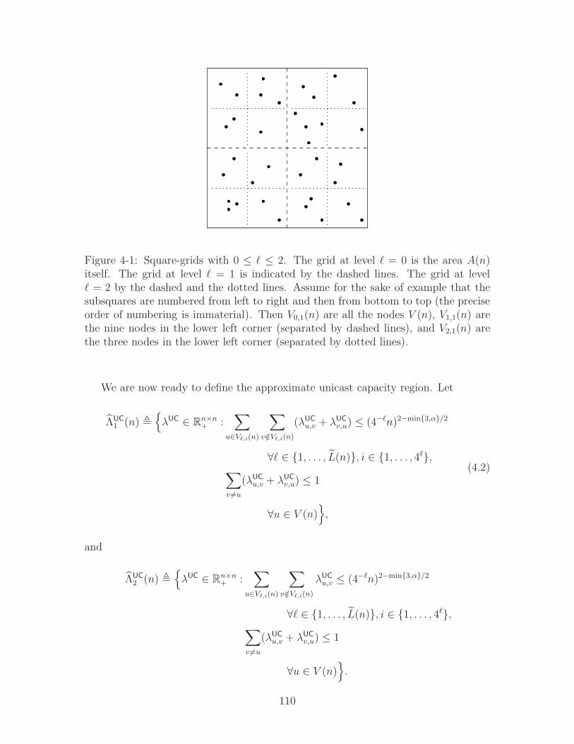
Figure 4-1: Square-grids with 0 ≤ ℓ ≤ 2. The grid at level ℓ = 0 is the area A(n)itself. The grid at level ℓ = 1 is indicated by the dashed lines. The grid at levelℓ = 2 by the dashed and the dotted lines. Assume for the sake of example that thesubsquares are numbered from left to right and then from bottom to top (the preciseorder of numbering is immaterial). Then V0,1(n) are all the nodes V (n), V1,1(n) arethe nine nodes in the lower left corner (separated by dashed lines), and V2,1(n) arethe three nodes in the lower left corner (separated by dotted lines).

We are now ready to define the approximate unicast capacity region. Let

ΛUC

1 (n) ,λUC ∈ R

n×n+ :

∑

u∈Vℓ,i(n)

∑

v/∈Vℓ,i(n)

(λUC

u,v + λUC

v,u) ≤ (4−ℓn)2−min3,α/2

∀ℓ ∈ 1, . . . , L(n), i ∈ 1, . . . , 4ℓ,∑

v 6=u

(λUC

u,v + λUC

v,u) ≤ 1

∀u ∈ V (n),

(4.2)

and

ΛUC

2 (n) ,λUC ∈ R

n×n+ :

∑

u∈Vℓ,i(n)

∑

v/∈Vℓ,i(n)

λUC

u,v ≤ (4−ℓn)2−min3,α/2

∀ℓ ∈ 1, . . . , L(n), i ∈ 1, . . . , 4ℓ,∑

v 6=u

(λUC

u,v + λUC

v,u) ≤ 1

∀u ∈ V (n).

110

ΛUC1 (n) and ΛUC

2 (n) are the collection of all unicast traffic matrices λUC such that for

various cuts S ⊂ V (n) in the network, the total traffic demand (in either one or both

directions)

∑

u∈S

∑

v/∈S

λUC

u,v,

∑

u∈S

∑

v/∈S

(λUC

u,v + λUC

v,u),

across the cut S is not too big. Note that the number of cuts S we need to consider is

actually quite small. In fact, there are at most n sets Vℓ,i(n)ℓ,i for ℓ ∈ 1, . . . , L(n).Hence ΛUC

1 (n) and ΛUC2 (n) are described by 2n cuts.

The next theorem shows that ΛUC1 (n) is an approximate (in the scaling sense)

inner bound and ΛUC2 (n) is an approximate outer bound to the unicast capacity region

ΛUC(n) of the wireless network.

Theorem 4.1. Under either fast or slow fading, for any α > 2, there exist

b1(n) ≥ n−o(1),

b2(n) = O(log6(n)),

such that

b1(n)ΛUC

1 (n) ⊂ ΛUC(n) ⊂ b2(n)ΛUC

2 (n),

with probability 1 − o(1) as n→ ∞.

We point out that Theorem 4.1 holds only with probability 1 − o(1) for different

reasons for the fast and slow fading cases. Under fast fading, the theorem holds only

for node placements that are “regular enough”. The node placement itself is random,

and we show that the required regularity property is satisfied with high probability as

n→ ∞. Under slow fading, the theorem holds under the same regularity requirements

on the node placement, but now it also only holds with high probability for the

realization of the fading θu,vu,v.

Comparing the expression for ΛUC1 (n) and ΛUC

2 (n), we see that whenever a traffic

111

matrix λUC satisfies

∑

u∈Vℓ,i(n)

∑

v/∈Vℓ,i(n)

(λUC

u,v + λUC

v,u) ≤ no(1)∑

u∈Vℓ,i(n)

∑

v/∈Vℓ,i(n)

λUC

u,v, (4.3)

for all ℓ ∈ 1, . . . , L(n) and i ∈ 1, . . . 4ℓ, then λUC ∈ ΛUC2 (n) implies n−o(1)λUC ∈

ΛUC1 (n), and hence for such traffic matrices the inner and outer bounds in Theorem

4.1 coincide in the scaling sense. In particular, this applies for traffic matrices λUC

such that (4.3) holds with equality, and we call such traffic (approximately) balanced

in the following. Note that the condition of balanced traffic imposes (less than) n

linear constraints on λUC, and hence Theorem 4.1 provides the correct scaling of the

n2-dimensional unicast capacity region ΛUC(n) along at least n2 − n dimensions.

In the high path-loss exponent regime (α > 5), it can be shown that ΛUC1 (n) is

also an approximate outer bound.

Theorem 4.2. Under either fast or slow fading, for any α > 5, there exists

b3(n) = O(log6(n)),

such that

ΛUC(n) ⊂ b3(n)ΛUC

1 (n),

with probability 1 − o(1) as n→ ∞.

Combining Theorems 4.1 and 4.2 provides a tight scaling characterization for

α > 5 of the entire unicast capacity region ΛUC(n) of the wireless network as depicted

in Figure 4-2. The approximations in both theorems are within a factor n±o(1). This

factor can be sharpened as is discussed in detail in Section 4.7.2.

4.1.2 Implications of Theorem 4.1 and 4.2

Theorems 4.1 and 4.2 can be applied in two ways. First, the theorems can be used to

analyze the asymptotic achievability of a sequence of traffic matrices. Let λUC(n)n≥1

112

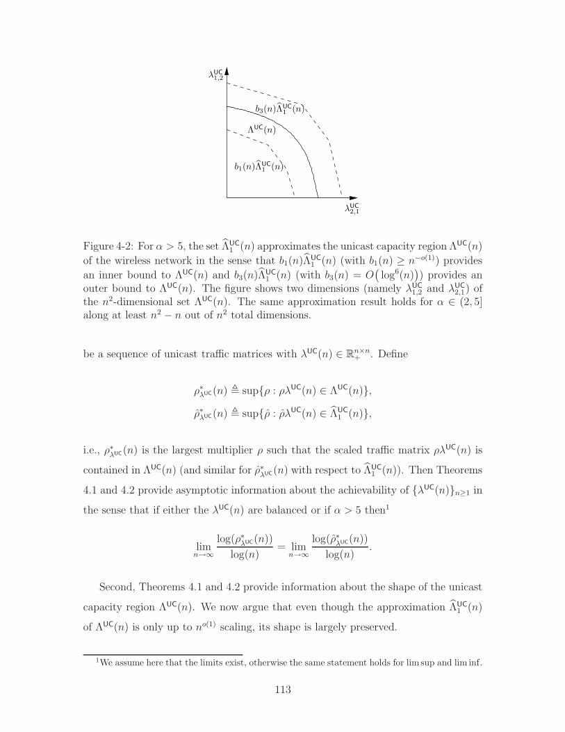
λUC1,2

λUC2,1

ΛUC(n)

b1(n)ΛUC1 (n)

b3(n)ΛUC1 (n)

Figure 4-2: For α > 5, the set ΛUC1 (n) approximates the unicast capacity region ΛUC(n)

of the wireless network in the sense that b1(n)ΛUC1 (n) (with b1(n) ≥ n−o(1)) provides

an inner bound to ΛUC(n) and b3(n)ΛUC1 (n) (with b3(n) = O

(log6(n)

)) provides an

outer bound to ΛUC(n). The figure shows two dimensions (namely λUC1,2 and λUC

2,1) ofthe n2-dimensional set ΛUC(n). The same approximation result holds for α ∈ (2, 5]along at least n2 − n out of n2 total dimensions.

be a sequence of unicast traffic matrices with λUC(n) ∈ Rn×n+ . Define

ρ∗λUC(n) , supρ : ρλUC(n) ∈ ΛUC(n),

ρ∗λUC(n) , supρ : ρλUC(n) ∈ ΛUC

1 (n),

i.e., ρ∗λUC(n) is the largest multiplier ρ such that the scaled traffic matrix ρλUC(n) is

contained in ΛUC(n) (and similar for ρ∗λUC(n) with respect to ΛUC1 (n)). Then Theorems

4.1 and 4.2 provide asymptotic information about the achievability of λUC(n)n≥1 in

the sense that if either the λUC(n) are balanced or if α > 5 then1

limn→∞

log(ρ∗λUC(n))

log(n)= lim

n→∞

log(ρ∗λUC(n))

log(n).

Second, Theorems 4.1 and 4.2 provide information about the shape of the unicast

capacity region ΛUC(n). We now argue that even though the approximation ΛUC1 (n)

of ΛUC(n) is only up to no(1) scaling, its shape is largely preserved.

1We assume here that the limits exist, otherwise the same statement holds for lim sup and lim inf.

113

To illustrate this point, consider a rectangle

R(n) , [0, r1(n)] × [0, r2(n)],

and let

R(n) , [0, r1(n)] × [0, r2(n)],

where

ri , bi(n)ri(n)

for some bi(n) = n±o(1), be its approximation. The shape of R(n) is then determined

by the ratio between r1(n) and r2(n). For example, assume r1(n) = nβr2(n). Then

r1(n)

r2(n)= nβ±o(1) = n±o(1) r1(n)

r2(n),

i.e.,

limn→∞

log(r1(n)/r2(n)

)

log(n)= β = lim

n→∞

log(r1(n)/r2(n)

)

log(n),

and hence the approximation R(n) preserves the exponent of the ratio of sidelengths

of R(n). In other words, if the two sidelengths r1(n) and r2(n) differ on exponential

scale (i.e., by a factor nβ for β 6= 0) then this shape information is preserved by the

approximation R(n).

Let us now return to the unicast capacity region ΛUC(n) and its approximation

ΛUC1 (n). We consider several boundary points of ΛUC(n) and show that their behavior

varies at scale nβ for different values of β. From the discussion in the previous

paragraph, this implies that a significant part of the shape of ΛUC(n) is preserved

by its approximation ΛUC1 (n). First, let λUC , ρ(n)1 for some scalar ρ(n) depending

only on n, and where 1 is the n × n matrix of all ones. If λUC ∈ ΛUC(n) then the

largest achievable value of ρ(n) is ρ∗(n) ≤ n−min3,α/2+o(1) (by applying Theorem

4.1). Second, let λUC such that λUCu∗,w∗ = ρ(n) for only one source-destination pair

(u∗, w∗) with u∗ 6= w∗ and λUCu,w = 0 otherwise. Then ρ∗(n), the largest achievable

value of ρ(n), satisfies ρ∗(n) ≥ n−o(1) (again by Theorem 4.1). Hence the boundary

114

points of ΛUC(n) vary at least from n−min3,α/2+o(1) to n−o(1), and this variation on

exponential scale is preserved by ΛUC1 (n).

4.1.3 Computational Aspects

Since we are interested in large wireless networks, computational aspects are of im-

portance. In this section, we show that the region ΛUC1 (n) can be efficiently described.

By Theorems 4.1 and 4.2, this provides a computationally efficient approximate de-

scription of the entire unicast capacity region ΛUC(n) for α > 5 and of n2 − n of its

n2 dimensions for α ∈ (2, 5].

Note that ΛUC(n) is a n2-dimensional set, and hence its shape could be rather

complex. In particular, in the special cases where the capacity region is known, its

description is often in terms of cut-set bounds. Since there are 2n possible subsets

of n nodes, there are 2n possible cut-set bounds to be considered. In other words,

the description complexity of ΛUC(n) is likely to be growing exponentially in n. On

the other hand, as was pointed out in Section 4.1.1, the description of ΛUC1 (n) is in

terms of only 2n cuts. This implies that ΛUC1 (n) can be computed efficiently (i.e., in

polynomial time in n). Hence even though the description complexity of ΛUC(n) is

likely to be of order Θ(2n), the description complexity of its approximation ΛUC1 (n)

is only of order Θ(n) — an exponential reduction. In particular, consider a unicast

traffic matrix λUC and assume that either α > 5 or that λUC is balanced, then this

implies that membership λUC ∈ ΛUC(n) (and hence by Theorems 4.1 and 4.2 also

the approximate achievability of the unicast traffic matrix λUC) can be computed in

polynomial time in the network size n. More precisely, evaluating each of the Θ(n)

cuts takes at most Θ(n2) operations, yielding a Θ(n3)-time algorithm for approximate

testing of membership in ΛUC(n).

4.2 Example Scenarios

We next illustrate the strength of the above results by determining achievable rates

in a few specific wireless network scenarios with non-uniform traffic patterns. We

115

illustrate the impact on achievable rates of various sources of traffic heterogeneities

— variation of distance between source-destination pairs, variation of amount of traffic

between different pairs, sources with multiple destinations.

Example 4.1. Multiple classes of source-destination pairs

There are K classes of source-destination pairs, for some fixed K. Each source

node in class i generates traffic at the same rate ρi(n) for a destination node that

is chosen randomly within distance Θ(nβi/2), for some fixed βi ∈ [0, 1]. Each node

randomly picks the class it belongs to. The resulting traffic matrix is approximately

balanced with high probability, and applying Theorem 4.1 shows that ρ∗i (n), the

largest achievable value of ρi(n), satisfies

ρ∗i (n) = nβi(1−α/2)±o(1),

with probability 1 − o(1) for all i, and where

α , min3, α.

Hence, for a fixed number of classes K, source nodes in each class can obtain rates

as a function of only the source-destination separation in that class.

Set ni , nβi , and note that ni is on the order of the expected number of nodes

that are closer to a source than its destination. Then

ρ∗i (n) = n±o(1)n1−α/2i .

Now n1−α/2i is precisely the per-node rate that is achievable for an extended network

with ni nodes under random source-destination pairing [38]. In other words, the local

traffic pattern here allows us to obtain a rate that is as good as the one achievable

under random source-destination pairing for a much smaller network. ♦

Example 4.2. Traffic variation with source-destination separation

Assume each node is source for exactly one destination chosen uniformly at random

from among all the other nodes (as in the traditional setting). However, instead of all

116

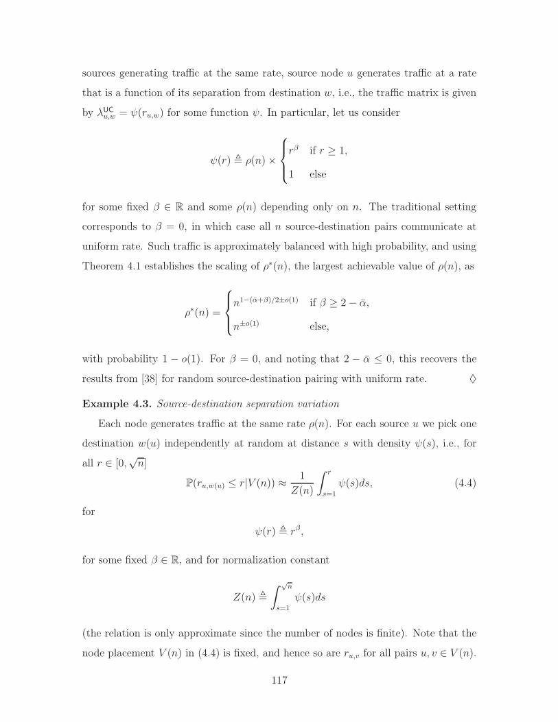
sources generating traffic at the same rate, source node u generates traffic at a rate

that is a function of its separation from destination w, i.e., the traffic matrix is given

by λUCu,w = ψ(ru,w) for some function ψ. In particular, let us consider

ψ(r) , ρ(n) ×

rβ if r ≥ 1,

1 else

for some fixed β ∈ R and some ρ(n) depending only on n. The traditional setting

corresponds to β = 0, in which case all n source-destination pairs communicate at

uniform rate. Such traffic is approximately balanced with high probability, and using

Theorem 4.1 establishes the scaling of ρ∗(n), the largest achievable value of ρ(n), as

ρ∗(n) =

n1−(α+β)/2±o(1) if β ≥ 2 − α,

n±o(1) else,

with probability 1 − o(1). For β = 0, and noting that 2 − α ≤ 0, this recovers the

results from [38] for random source-destination pairing with uniform rate. ♦

Example 4.3. Source-destination separation variation

Each node generates traffic at the same rate ρ(n). For each source u we pick one

destination w(u) independently at random at distance s with density ψ(s), i.e., for

all r ∈ [0,√n]

P(ru,w(u) ≤ r|V (n)) ≈ 1

Z(n)

∫ r

s=1

ψ(s)ds, (4.4)

for

ψ(r) , rβ,

for some fixed β ∈ R, and for normalization constant

Z(n) ,

∫ √n

s=1

ψ(s)ds

(the relation is only approximate since the number of nodes is finite). Note that the

node placement V (n) in (4.4) is fixed, and hence so are ru,v for all pairs u, v ∈ V (n).

117

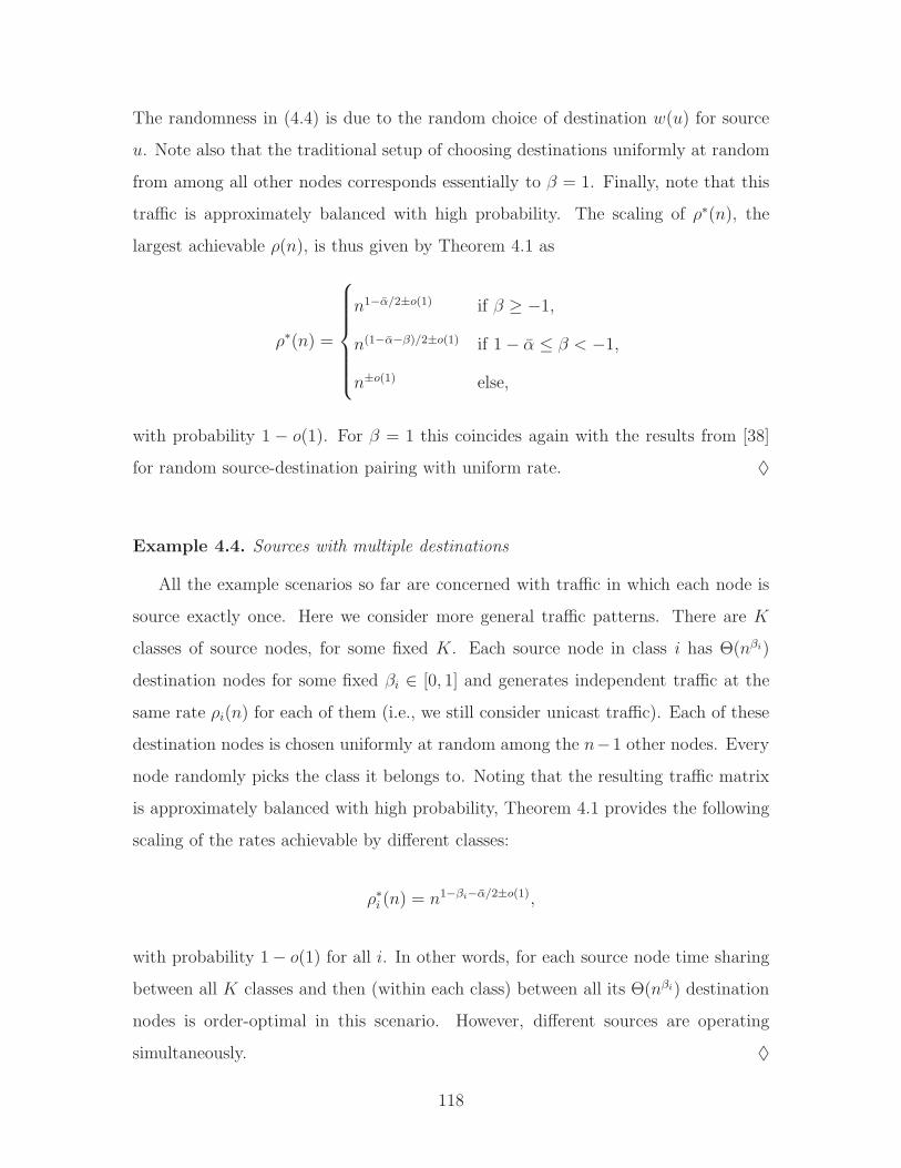
The randomness in (4.4) is due to the random choice of destination w(u) for source

u. Note also that the traditional setup of choosing destinations uniformly at random

from among all other nodes corresponds essentially to β = 1. Finally, note that this

traffic is approximately balanced with high probability. The scaling of ρ∗(n), the

largest achievable ρ(n), is thus given by Theorem 4.1 as

ρ∗(n) =

n1−α/2±o(1) if β ≥ −1,

n(1−α−β)/2±o(1) if 1 − α ≤ β < −1,

n±o(1) else,

with probability 1 − o(1). For β = 1 this coincides again with the results from [38]

for random source-destination pairing with uniform rate. ♦

Example 4.4. Sources with multiple destinations

All the example scenarios so far are concerned with traffic in which each node is

source exactly once. Here we consider more general traffic patterns. There are K

classes of source nodes, for some fixed K. Each source node in class i has Θ(nβi)

destination nodes for some fixed βi ∈ [0, 1] and generates independent traffic at the

same rate ρi(n) for each of them (i.e., we still consider unicast traffic). Each of these

destination nodes is chosen uniformly at random among the n−1 other nodes. Every

node randomly picks the class it belongs to. Noting that the resulting traffic matrix

is approximately balanced with high probability, Theorem 4.1 provides the following

scaling of the rates achievable by different classes:

ρ∗i (n) = n1−βi−α/2±o(1),

with probability 1 − o(1) for all i. In other words, for each source node time sharing

between all K classes and then (within each class) between all its Θ(nβi) destination

nodes is order-optimal in this scenario. However, different sources are operating

simultaneously. ♦

118

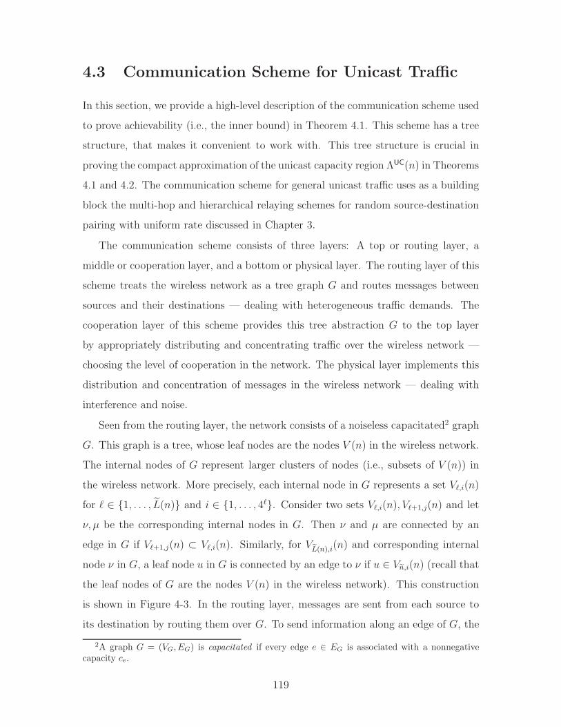
4.3 Communication Scheme for Unicast Traffic

In this section, we provide a high-level description of the communication scheme used

to prove achievability (i.e., the inner bound) in Theorem 4.1. This scheme has a tree

structure, that makes it convenient to work with. This tree structure is crucial in

proving the compact approximation of the unicast capacity region ΛUC(n) in Theorems

4.1 and 4.2. The communication scheme for general unicast traffic uses as a building

block the multi-hop and hierarchical relaying schemes for random source-destination

pairing with uniform rate discussed in Chapter 3.

The communication scheme consists of three layers: A top or routing layer, a

middle or cooperation layer, and a bottom or physical layer. The routing layer of this

scheme treats the wireless network as a tree graph G and routes messages between

sources and their destinations — dealing with heterogeneous traffic demands. The

cooperation layer of this scheme provides this tree abstraction G to the top layer

by appropriately distributing and concentrating traffic over the wireless network —

choosing the level of cooperation in the network. The physical layer implements this

distribution and concentration of messages in the wireless network — dealing with

interference and noise.

Seen from the routing layer, the network consists of a noiseless capacitated2 graph

G. This graph is a tree, whose leaf nodes are the nodes V (n) in the wireless network.

The internal nodes of G represent larger clusters of nodes (i.e., subsets of V (n)) in

the wireless network. More precisely, each internal node in G represents a set Vℓ,i(n)

for ℓ ∈ 1, . . . , L(n) and i ∈ 1, . . . , 4ℓ. Consider two sets Vℓ,i(n), Vℓ+1,j(n) and let

ν, µ be the corresponding internal nodes in G. Then ν and µ are connected by an

edge in G if Vℓ+1,j(n) ⊂ Vℓ,i(n). Similarly, for VeL(n),i(n) and corresponding internal

node ν in G, a leaf node u in G is connected by an edge to ν if u ∈ Ven,i(n) (recall that

the leaf nodes of G are the nodes V (n) in the wireless network). This construction

is shown in Figure 4-3. In the routing layer, messages are sent from each source to

its destination by routing them over G. To send information along an edge of G, the

2A graph G = (VG, EG) is capacitated if every edge e ∈ EG is associated with a nonnegativecapacity ce.

119

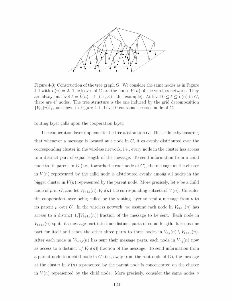
Figure 4-3: Construction of the tree graphG. We consider the same nodes as in Figure4-1 with L(n) = 2. The leaves of G are the nodes V (n) of the wireless network. They

are always at level ℓ = L(n) + 1 (i.e., 3 in this example). At level 0 ≤ ℓ ≤ L(n) in G,there are 4ℓ nodes. The tree structure is the one induced by the grid decompositionVℓ,i(n)ℓ,i as shown in Figure 4-1. Level 0 contains the root node of G.

routing layer calls upon the cooperation layer.

The cooperation layer implements the tree abstraction G. This is done by ensuring

that whenever a message is located at a node in G, it es evenly distributed over the

corresponding cluster in the wireless network, i.e., every node in the cluster has access

to a distinct part of equal length of the message. To send information from a child

node to its parent in G (i.e., towards the root node of G), the message at the cluster

in V (n) represented by the child node is distributed evenly among all nodes in the

bigger cluster in V (n) represented by the parent node. More precisely, let ν be a child

node of µ in G, and let Vℓ+1,i(n), Vℓ,j(n) the corresponding subsets of V (n). Consider

the cooperation layer being called by the routing layer to send a message from ν to

its parent µ over G. In the wireless network, we assume each node in Vℓ+1,i(n) has

access to a distinct 1/|Vℓ+1,i(n)| fraction of the message to be sent. Each node in

Vℓ+1,i(n) splits its message part into four distinct parts of equal length. It keeps one

part for itself and sends the other three parts to three nodes in Vℓ,j(n) \ Vℓ+1,i(n).

After each node in Vℓ+1,i(n) has sent their message parts, each node in Vℓ,j(n) now

as access to a distinct 1/|Vℓ,j(n)| fraction of the message. To send information from

a parent node to a child node in G (i.e., away from the root node of G), the message

at the cluster in V (n) represented by the parent node is concentrated on the cluster

in V (n) represented by the child node. More precisely, consider the same nodes ν

120

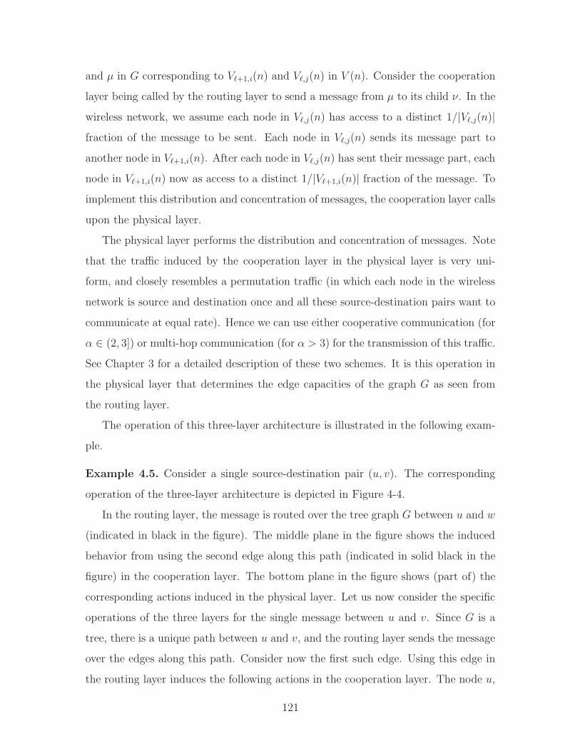
and µ in G corresponding to Vℓ+1,i(n) and Vℓ,j(n) in V (n). Consider the cooperation

layer being called by the routing layer to send a message from µ to its child ν. In the

wireless network, we assume each node in Vℓ,j(n) has access to a distinct 1/|Vℓ,j(n)|fraction of the message to be sent. Each node in Vℓ,j(n) sends its message part to

another node in Vℓ+1,i(n). After each node in Vℓ,j(n) has sent their message part, each

node in Vℓ+1,i(n) now as access to a distinct 1/|Vℓ+1,i(n)| fraction of the message. To

implement this distribution and concentration of messages, the cooperation layer calls

upon the physical layer.

The physical layer performs the distribution and concentration of messages. Note

that the traffic induced by the cooperation layer in the physical layer is very uni-

form, and closely resembles a permutation traffic (in which each node in the wireless

network is source and destination once and all these source-destination pairs want to

communicate at equal rate). Hence we can use either cooperative communication (for

α ∈ (2, 3]) or multi-hop communication (for α > 3) for the transmission of this traffic.

See Chapter 3 for a detailed description of these two schemes. It is this operation in

the physical layer that determines the edge capacities of the graph G as seen from

the routing layer.

The operation of this three-layer architecture is illustrated in the following exam-

ple.

Example 4.5. Consider a single source-destination pair (u, v). The corresponding

operation of the three-layer architecture is depicted in Figure 4-4.

In the routing layer, the message is routed over the tree graph G between u and w

(indicated in black in the figure). The middle plane in the figure shows the induced

behavior from using the second edge along this path (indicated in solid black in the

figure) in the cooperation layer. The bottom plane in the figure shows (part of) the

corresponding actions induced in the physical layer. Let us now consider the specific

operations of the three layers for the single message between u and v. Since G is a

tree, there is a unique path between u and v, and the routing layer sends the message

over the edges along this path. Consider now the first such edge. Using this edge in

the routing layer induces the following actions in the cooperation layer. The node u,

121

u

w

Figure 4-4: Example operation of the three-layer architecture under unicast traffic.The three layers depicted are (from top to bottom in the figure) the routing layer,the cooperation layer, and the physical layer.

122

having access to the entire message, splits that message into 3 distinct parts of equal

length. It keeps one part, and sends the other two parts to the two other nodes in

V2,1(n) (i.e., lower left square at level ℓ = 2 in the hierarchy). In other words, after the

message has traversed the edge between u and its parent node in the routing layer, all

nodes in V2,1(n) in the cooperation layer have access to a distinct 1/3 fraction of the

original message. The edges in the routing layer leading up the tree (i.e., towards the

root node) are implemented in the cooperation layer in a similar fashion by further

distributing the message over the wireless network. By the time the message reaches

the root node of G in the routing layer, the cooperation layer has distributed the

message over the entire network and every node in V (n) has access to a distinct 1/n

fraction of the original message. Communication down the tree in the routing layer is

implemented in the cooperation layer by concentrating messages over smaller regions

in the wireless network. To physically perform this distribution and concentration

of messages, the cooperation layer calls upon the physical layer, which uses either

hierarchical relaying or multi-hop communication. ♦

4.4 Auxiliary Lemmas

In this section, we provide auxiliary results, which will be used several times in the

following. These results are grouped into three parts. In Section 4.4.1, we describe

regularity properties exhibited with high probability by the random node placement.

In Section 4.4.2, we provide auxiliary upper bounds on the performance of any scheme

in terms of cut-set bounds. Finally, in Section 4.4.3, we describe auxiliary results on

the performance of hierarchical relaying and multi-hop communication.

4.4.1 Regularity Lemmas

Here we prove several regularity properties that are satisfied with high probability

by a random node placement. Formally, define V(n) to be the collection of all node

123

placements V (n) that satisfy the following conditions:

ru,v > n−1 ∀u, v ∈ V (n),

∣∣Vℓ,i(n)∣∣ ≤ log(n) for ℓ =

1

2log(n) and ∀i ∈ 1, . . . , 4ℓ,

∣∣Vℓ,i(n)∣∣ ≥ 1 for ℓ =

1

2log( n

2 log(n)

)and ∀i ∈ 1, . . . , 4ℓ,

∣∣Vℓ,i(n)∣∣ ∈ [4−ℓ−1n, 4−ℓ+1n] ∀ℓ ∈

1, . . . ,

1

2log(n)

(1 − log−5/6(n)

), i ∈ 1, . . . , 4ℓ.

The first condition is that the minimum separation between node pairs is not too

small. The second condition is that all squares of area 1 contain at most log(n)

nodes. The third condition is that all squares of area 2 log(n) contain at least one

node. The fourth condition is that all squares up to level 12log(n)

(1 − log−5/6(n)

)

contain a number of nodes proportional to their area. Note that, since

L(n) ≤ 1

2log(n)

(1 − log5/6(n)

),

this holds in particular for nodes up to level L(n). The goal of this section is to prove

that

P(V (n) ∈ V(n)) = 1 − o(1),

as n→ ∞.

The first lemma shows that the minimum separation in a random node placement

is at least n−1 with high probability.

Lemma 4.3.

P

(min

u∈V (n),v∈V (n)\uru,v > n−1

)= 1 − o(1),

as n→ ∞.

Proof. For u, v ∈ V , let

Bu,v , ru,v ≤ r

124

for some r (depending only on n). Fix a node u ∈ V , then

P(Bu,v|u) ≤r2π

n,

(the inequality being due to boundary effects). Moreover, the events Bu,vv∈V \u

are independent conditioned on u, and thus

P

(∩v∈V \u B

cu,v

∣∣u)

=∏

v∈V \uP(Bc

u,v|u) ≥(1 − r2π

n

)n

.

From this,

P

(min

u∈V,v∈V \uru,v ≤ r

)= P

(∪u∈V,v∈V \u Bu,v

)

≤∑

u∈V

P

(∪v∈V \u Bu,v

)

=∑

u∈V

(1 − P

(∩v∈V \u B

cu,v

))

=∑

u∈V

(1 − E

(P

(∩v∈V \u B

cu,v

∣∣u)))

≤∑

u∈V

(1 −

(1 − r2π

n

)n)

= n(1 −

(1 − r2π

n

)n),

which converges to zero for r = n−1.

The next lemma asserts that if ℓ(n) is not too large then all squares Vℓ,i(n)ℓ,i

for ℓ ∈ 1, . . . , ℓ(n) and i ∈ 1, . . . , 4ℓ in the grid decomposition of V (n) contain a

number of nodes that is proportional to their area.

Lemma 4.4. If ℓ(n) satisfies

limn→∞

ℓ(n)

4−ℓ(n)n= 0

125

then

P

( ℓ(n)⋂

ℓ=1

4ℓ⋂

i=1

|Vℓ,i(n)| ∈ [4−ℓ−1n, 4−ℓ+1n]

)= 1 − o(1)

as n→ ∞. In particular, this holds for

ℓ(n) =1

2log(n)

(1 − log−5/6(n)

),

and for ℓ(n) = L(n).

Proof. Let Bu be the event that node u lies in Aℓ,i for fixed ℓ, i. Note that

∑

u∈V

11Bu = |Vℓ,i|

by definition, and that

P(Bu) = 4−ℓ.

Hence using the Chernoff bound

P

(∑

u∈V

11Bu 6∈ [4−ℓ−1n, 4−ℓ+1n]

)≤ exp(−K4−ℓn),

for some constant K. From this, we obtain for ℓ = ℓ(n),

P

( 4ℓ(n)⋂

i=1

|Vℓ(n),i| ∈ [4−ℓ(n)−1n, 4−ℓ(n)+1n]

)

≥ 1 −4ℓ(n)∑

i=1

P(|Vℓ(n),i| 6∈ [4−ℓ(n)−1n, 4−ℓ(n)+1n]

)

≥ 1 − 4ℓ(n) exp(−K4−ℓ(n)n)

≥ 1 − exp(Kℓ(n) −K4−ℓ(n)n),

(4.5)

for some constant K. By assumption

limn→∞

ℓ(n)

4−ℓ(n)n= 0,

126

and hence

P

( 4ℓ(n)⋂

i=1

|Vℓ(n),i| ∈ [4−ℓ(n)−1n, 4−ℓ(n)+1n]

)≥ 1 − o(1),

as n→ ∞. Since the Aℓ,iℓ,i are nested as a function of ℓ, we have

ℓ(n)⋂

ℓ=1

4ℓ⋂

i=1

|Vℓ,i| ∈ [4−ℓ−1n, 4−ℓ+1n]

=

4ℓ(n)⋂

i=1

|Vℓ(n),i| ∈ [4−ℓ(n)−1n, 4−ℓ(n)+1n]

,

which, combined with (4.5), proves the first part of the lemma.

For the second part, note that for

ℓ(n) =1

2log(n)

(1 − log−5/6(n)

),

we have

ℓ(n)

4−ℓ(n)n=

12log(n)

(1 − log−5/6(n)

)

2log1/6(n)

≤ log(n)

2log1/6(n)

= 2log log(n)−log1/6(n) → 0,

and hence the lemma is valid in this case. The same holds for ℓ(n) = L(n) since

L(n) ≤ 1

2log(n)

(1 − log−5/6(n)

).

We are now ready to prove that a random node placement V (n) is in V(n) with

high probability as n→ ∞ (i.e., is fairly “regular” with high probability).

Lemma 4.5.

P(V (n) ∈ V(n)) = 1 − o(1),

as n→ ∞.

127

Proof. The first condition,

ru,v > n−1 ∀u, v ∈ V ,

holds with probability 1 − o(1) by Lemma 4.3. The second and third conditions,

∣∣Vℓ,i

∣∣ ≤ log(n) for ℓ =1

2log(n) and ∀i ∈ 1, . . . , 4ℓ,

∣∣Vℓ,i

∣∣ ≥ 1 for ℓ =1

2log( n

2 log(n)

)and ∀i ∈ 1, . . . , 4ℓ,

are shown in [38, Lemma 5.1] to hold with probability 1−o(1). The fourth condition,

∣∣Vℓ,i

∣∣ ∈ [4−ℓ−1n, 4−ℓ+1n] ∀ℓ ∈

1, . . . ,1

2log(n)

(1 − log−5/6(n)

), i ∈ 1, . . . , 4ℓ,

holds with probability 1 − o(1) by Lemma 4.4. Together, this proves the desired

result.

4.4.2 Converse Lemmas

Here we prove several auxiliary converse results. The first lemma bounds the maximal

achievable sum rate for every individual node (i.e., the total traffic for which a fixed

node is either source or destination).

Lemma 4.6. Under either fast or slow fading, for any α > 2, there exists b(n) =

O(log(n)) such that for all V (n) ∈ V(n), λUC ∈ ΛUC(n), u ∈ V (n),

∑

v∈V (n)\uλUC

u,v ≤ b(n), (4.6)

∑

v∈V (n)\uλUC

v,u ≤ b(n). (4.7)

Proof. The argument follows the one in [38, Theorem 3.1]. For any S1, S2 ⊂ V , denote

by C(S1, S2) the MIMO capacity between nodes in S1 and nodes in S2. Consider first

128

(4.6). By the cut-set bound [9, Theorem 14.10.1],

∑

v 6=u

λUC

u,v ≤ C(u, uc).

Here C(u, uc) is the SIMO capacity between u and the nodes in uc, i.e.,

C(u, uc) = log(1 +

∑v 6=u|hu,v|2

)

≤ log(1 + (n− 1)nα)

≤ K log(n),

with

K , 2 + α,

and where for the first inequality we have used that since V ∈ V, we have ru,v ≥ n−1

for all u, v ∈ V .

Similarly, for (4.7),∑

v 6=u

λUC

v,u ≤ C(uc, u),

and

C(uc, u) ≤ log(1 + (n− 1)

∑v 6=u|hv,u|2

)

≤ log(1 + (n− 1)2nα)

≤ K log(n).

The next two lemmas bounds the maximal achievable sum rate across the bound-

ary of the subsquares Vℓ,i(n) for ℓ ∈ 1, . . . , L(n), and i ∈ 1, . . . , 4ℓ.

Lemma 4.7. Under either fast or slow fading, for any α > 2, there exists b(n) =

O(log6(n)

)such that for all V (n) ∈ V(n), λUC ∈ ΛUC(n), ℓ ∈ 1, . . . , L(n), and

129

i ∈ 1, . . . , 4ℓ, we have

∑

u∈Vℓ,i(n)

∑

v/∈Vℓ,i(n)

λUC

u,v ≤ b(n)(4−ℓn)2−min3,α/2.

Proof. As before, denote by C(S1, S2) the MIMO capacity between nodes in S1 and

nodes in S2, for S1, S2 ⊂ V . By the cut-set bound [9, Theorem 14.10.1],

∑

u∈Vℓ,i

∑

v/∈Vℓ,i

λUC

u,v ≤ C(Vℓ,i, Vcℓ,i). (4.8)

Let

HS1,S2 , [hu,v]u∈S1,v∈S2

be the matrix of channel gains between the nodes in S1 and S2. Under fast fading

C(S1, S2) , maxQ(H)≥0:

E(qu,u)≤P ∀u∈S1

E

(log det

(I + H

†S1,S2

Q(H)HS1,S2

)),

and under slow fading

C(S, Sc) , maxQ≥0:

qu,u≤P ∀u∈S1

log det(I + H

†S1,S2

QHS1,S2

).

Denote by ∂(V cℓ,i) the nodes in V c

ℓ,i that are within distance 8(√

2 log(n) + 1) of the

boundary between Acℓ,i and Aℓ,i. Using the generalized Hadamard’s inequality, yields

then that under either fast or slow fading

C(Vℓ,i, Vcℓ,i) ≤ C(Vℓ,i, ∂(V

cℓ,i)) + C(Vℓ,i, V

cℓ,i \ ∂(V c

ℓ,i)). (4.9)

We start by analyzing the first term in the sum in (4.9). Applying Hadamard’s

inequality again yields

C(Vℓ,i, ∂(Vcℓ,i)) ≤

∑

v∈∂(V cℓ,i)

C(Vℓ,i, v).

130

Since V ∈ V, we have

|∂(V cℓ,i)| ≤ 40 log(n)(

√2 log(n) + 1)(4−ℓn)1/2 ≤ 120 log2(n)(4−ℓn)1/2

and by the same analysis as in Lemma 4.6, we have

C(Vℓ,i, v) ≤ C(vc, v) ≤ K

120log(n)

for some constant K (independent of v). Therefore

C(Vℓ,i, ∂(Vcℓ,i)) ≤ 120 log(n)2(4−ℓn)1/2 K

120log(n)

≤ K log3(n)(4−ℓn)1/2. (4.10)

We now analyze the second term in the sum in (4.9). Applying Lemma 3.12,

C(Vℓ,i, Vcℓ,i \ ∂(V c

ℓ,i))

≤ 4 max

1, maxv∈V c

ℓ,i\∂(V cℓ,i)

∑

u∈Vℓ,i

r−αu,v∑

v∈V cℓ,i\∂(V c

ℓ,i)r−αu,v

∑

u∈Vℓ,i

∑

v∈V cℓ,i\∂(V c

ℓ,i)

r−αu,v . (4.11)

We now show that the term in parentheses in (4.11) is O(log3(n)). Fix u ∈ Vℓ,i and

denote by du the distance of u to the closest point in V cℓ,i \ ∂(V c

ℓ,i). Note that be

definition of ∂(V cℓ,i), we have

du ≥ 8(√

2 log(n) + 1).

Since, V ∈ V, there are at least

d2u − 4du(

√2 log(n) + 1)

2 log(n)≥ d2

u

4 log(n)

131

nodes that are at distance at most 3du. Hence

∑

v∈V cℓ,i\∂(V c

ℓ,i)

r−αu,v ≥ d2−α

u

41+α log(n),

and therefore for any v ∈ V cℓ,i \ ∂(V c

ℓ,i),

r−αu,v∑

v∈V cℓ,i\∂(V c

ℓ,i)r−αu,v

≤ 41+α log(n)r−αu,v

d2−αu

≤ 41+α log(n)r−2u,v

(ru,v

du

)2−α

≤ 41+α log(n)r−2u,v.

(4.12)

Using V ∈ V, yields that for any v ∈ V cℓ,i \ ∂(V c

ℓ,i),

∑

u∈Vℓ,i

r−αu,v∑

v∈V cℓ,i\∂(V c

ℓ,i)r−αu,v

≤ 41+α log(n)∑

u∈Vℓ,i

r−2u,v ≤ 43+α ln(2) log3(n).

Combined with (4.11), this shows that

C(Vℓ,i, Vcℓ,i \ ∂(V c

ℓ,i)) ≤ K ′ log3(n)∑

u∈Vℓ,i

∑

v∈V cℓ,i

r−αu,v (4.13)

for some constant K ′ (independent of ℓ, and i).

Combining (4.10) and (4.13) with (4.9), we obtain

C(Vℓ,i, Vcℓ,i) ≤ K ′ log3(n)

∑

u∈Vℓ,i

∑

v∈V cℓ,i\∂(V c

ℓ,i)

r−αu,v +K log3(n)(4−ℓn)1/2. (4.14)

Moreover, using again the same arguments as in [38, Theorem 5.2] shows that there

exists a constant K such that for adjacent squares (i.e., sharing a side) Aℓ,i, Aℓ,j,

∑

u∈Vℓ,i

∑

v∈Vℓ,j\∂(V cℓ,i)

r−αu,v ≤ K log3(n)(4−ℓn)2−min3,α/2. (4.15)

Consider now two diagonal squares (i.e., sharing a corner point) Aℓ,i, Aℓ,j, and choose

132

ı, such that Aℓ,i ∪ Aℓ,ı and Aℓ,j ∪ Aℓ, are adjacent rectangles. Using the same

arguments to these rectangles and suitably redefining K shows that (4.15) holds for

diagonal squares as well.

Using this, we now compute the summation in (4.14). Consider “rings” of squares

around Aℓ,i. The first such “ring” contains the (at most) 8 squares neighboring Aℓ,i.

The next “ring” contains at most 16 squares. In general, “ring” k contains at most

8k squares. Let

Aℓ,jj∈Ik

be the squares in “ring” k. Then

∑

u∈Vℓ,i

∑

v∈V cℓ,i\∂(V c

ℓ,i)

r−αu,v =

∑

k≥1

∑

j∈Ik

∑

u∈Vℓ,i

∑

v∈Vℓ,j\∂(V cℓ,i)

r−αu,v . (4.16)

By (4.15),∑

j∈I1

∑

u∈Vℓ,i

∑

v∈Vℓ,j\∂(V cℓ,i)

r−αu,v ≤ 8K log3(n)(4−ℓn)2−min3,α/2. (4.17)

Now note that for k > 1 and j ∈ Ik, nodes u ∈ Vℓ,i and v ∈ Vℓ,j are at least at distance

ru,v ≥ (k − 1)(2−ℓ√n). Moreover, since V ∈ V, each Vℓ,jℓ,j has cardinality at most

4−ℓ+1n. Thus

∑

k>1

∑

j∈Ik

∑

u∈Vℓ,i

∑

v∈Vℓ,j\∂(V cℓ,i)

r−αu,v ≤

∑

k>1

8k(4−ℓ+1n

)2((k − 1)(2−ℓ

√n))−α

= 128(4−ℓn

)2−α/2∑

k>1

k(k − 1)−α

= K ′′(4−ℓn)2−α/2

, (4.18)

for some K ′′ > 0, and where we have used that α > 2. Substituting (4.17) and (4.18)

into (4.16) yields

∑

u∈Vℓ,i

∑

v∈V cℓ,i\∂(V c

ℓ,i)

r−αu,v ≤ 8K log3(n)(4−ℓn)2−min3,α/2 +K ′′(4−ℓn

)2−α/2. (4.19)

133

Combining (4.19) with (4.14) and (4.8) shows that

∑

u∈Vℓ,i

∑

v/∈Vℓ,i

λUC

u,v ≤ b(n)(4−ℓn)2−min3,α/2.

for every ℓ ∈ 1, . . . , L(n), i ∈ 1, . . . , 4ℓ, and under either fast or slow fading.

Lemma 4.8. Under either fast or slow fading, for any α > 5, there exists b(n) =

O(log3(n)

)such that for all V (n) ∈ V(n), λUC ∈ ΛUC(n), ℓ ∈ 1, . . . , L(n), and

i ∈ 1, . . . , 4ℓ, we have

∑

u/∈Vℓ,i(n)

∑

v∈Vℓ,i(n)

λUC

u,v ≤ b(n)(4−ℓn)1/2.

Proof. By the cut-set bound [9, Theorem 14.10.1],

∑

u/∈Vℓ,i

∑

v∈Vℓ,i

λUC

u,v ≤ C(V cℓ,i, Vℓ,i). (4.20)

Denote by ∂Vℓ,i the nodes in Vℓ,i that are within distance one of the boundary between

Acℓ,i and Aℓ,i. Applying the generalized Hadamard inequality as in Lemma 4.7, we

have under either fast or slow fading

C(V cℓ,i, Vℓ,i) ≤ C(V c

ℓ,i, ∂Vℓ,i) + C(V cℓ,i, Vℓ,i \ ∂Vℓ,i)

≤ K log3(n)(4−ℓn)1/2 + C(V cℓ,i, Vℓ,i \ ∂Vℓ,i),

(4.21)

for some constant K.

For the second term in (4.21), we have the following upper bound from Theorem

2.1 in [21]:

C(V cℓ,i, Vℓ,i \ ∂Vℓ,i) ≤

∑

v∈Vℓ,i\∂Vℓ,i

( ∑

u∈V cℓ,i

r−α/2u,v

)2

.

Now, consider v ∈ Vℓ,i \ ∂Vℓ,i and let dv be the distance of v to the closest node in

134

V cℓ,i. Then, using V ∈ V,

∑

u∈V cℓ,i

r−α/2u,v ≤ K log(n)d2−α/2

v ,

for some constant K, and hence for α > 5,

C(V cℓ,i, Vℓ,i \ ∂Vℓ,i) ≤

∑

v∈Vℓ,i\∂Vℓ,i

K2 log2(n)d4−αv

≤ K ′ log3(n)(4−ℓn)1/2.

Combined with (4.21), this proves Lemma 4.8 for traffic from V cℓ,i to Vℓ,i.

4.4.3 Achievability Lemmas

In this section, we prove auxiliary achievability results. Recall that a permutation

traffic is a traffic pattern in which each node is source and destination exactly once.

Call the corresponding source-destination pairing Π ⊂ V (n) × V (n) a permutation

pairing. The lemma below analyzes the performance achievable with either hier-

archical relaying (for α ∈ (2, 3]) or multi-hop communication (for α > 3) applied

simultaneously to transmit permutation traffic in several disjoint regions in the net-

work.

Lemma 4.9. Under fast fading, for any α > 2, there exists b(n) ≥ n−o(1) such that

for all V (n) ∈ V(n), ℓ ∈ 0, . . . , L(n), i ∈ 1, . . . , 4ℓ, and all permutation source-

destination pairings Πi on Vℓ,i(n), there exists λUC ∈ ΛUC(n) such that

mini∈1,...,4ℓ

min(u,v)∈Πi

λUC

u,v ≥ b(n)(4−ℓn)1−min3,α/2.

The same statement holds with probability 1−o(1) as n→ ∞ in the slow fading case.

Consider the source-destination pairing Π , ∪iΠi with Πi as in Lemma 4.9. This

is a permutation pairing, since each Πi is a permutation pairing on Vℓ,i(n) and since

the Vℓ,i(n)i are disjoint. Lemma 4.9 states that all source-destination pairs in Π

135

can communicate at a per-node rate of at least n−o(1)(4−ℓn)1−min3,α/2. Note that,

due to the locality of the traffic pattern, this can be considerably better than the

n1−min3,α/2−o(1) per-node rate achieved by standard hierarchical relaying or multi-

hop communication.

Proof. We shall use either hierarchical relaying (for α ∈ (2, 3]) or multi-hop (for

α > 3) to communicate within each square Vℓ,i. We operate every fourth of the Vℓ,i

simultaneously, and show that the added interference due to this spatial re-use results

only in a constant factor loss in rate.

Consider first α ∈ (2, 3] and fast fading. The squares Aℓ,i at level ℓ have an area

of

aℓ , 4−ℓn.

We will use hierarchical relaying within each of the Aℓ,ii. Applying Theorem 3.1)

with δ = 1/4, it is sufficient to show that we can partition each Aℓ,i into

a1

1+log−1/4(aℓ)

ℓ

subsquares, each of which contains a number of nodes proportional to the area (see

Section 3.10.4). In other words, we partition A into subsquares of size

a1− 1

1+log−1/4(aℓ)

ℓ ≥ alog−1/4(n)

1+log−1/4(n)

eL(n)

≥ alog−1/3(n)eL(n)

= nlog−5/6(n)

≥ n4− log(n)(1−log−5/6(n)).

Since V ∈ V, all these subsquares contain a number of nodes proportional to their

area, and hence this shows that all

Ai,ℓℓ∈0,...,eL(n),i∈1,...,4ℓ

136

are simultaneously regular enough for hierarchical relaying to be successful under fast

fading. By Theorem 3.1, this achieves a per-node rate of

λUC

u,v ≥ n−o(1)(4−ℓn)1−α/2 (4.22)

for any (u, v) ∈ Πi.

We now show that (4.22) holds with high probability also under slow fading. By

Theorem 3.1, for V ∈ V hierarchical relaying is successful under slow fading for all

permutation traffic on V with probability at least

1 − exp(− 2K log3/4(n)

)

for some constant K. Hence, hierarchical relaying is successful for all permutation

traffic on Vℓ,i with probability at least

1 − exp(− 2K log3/4(4−ℓn)

)≥ 1 − exp

(− 2K log3/4(4−

eL(n)n))

= 1 − exp(− 2K log3/8(n)

).

And hence hierarchical relaying is successful under slow fading for all ℓ ∈ 1, . . . , L(n)and all permutation traffic on every Vℓ,i4ℓ

i=1 with probability at least

1 − L(n)4eL(n) exp

(− 2K log3/8(n)

)≥ 1 − n2 exp

(− 2K log3/8(n)

)

≥ 1 − o(1)

as n→ ∞.

We now argue that the additional interference from spatial re-use results only in a

constant loss in rate. This follows from the same arguments as in the proof of Theorem

3.1 (with the appropriate modifications for slow fading as described there). Intuitively,

this is the case since the interference from a square at distance r is attenuated by a

factor r−α, which, since α > 2, is summable. Hence the combined interference has

power on the order of the receiver noise, resulting in only a constant factor loss in

137

rate.

For α > 3, the argument is similar — instead of hierarchical relaying we now

use multi-hop communication. For V ∈ V and under either fast or slow fading, this

achieves a per-node rate of

λUC

u,v ≥ n−o(1)(4−ℓn)−1/2 (4.23)

for any (u, v) ∈ Πi. Combining (4.22) and (4.23) yields the desired result.

4.5 Proof of Theorem 4.1

The proof of Theorem 4.1 relies on the construction of a capacitated (noiseless, wire-

line) graph G and linking its performance under routing to the performance of the

wireless network. This graph G = (VG, EG) is constructed as follows. G is a full tree

(i.e., all its leaf nodes are on the same level). G has n leaves, each of them represent-

ing an element of V (n). To simplify notation, we assume that V (n) ⊂ VG, so that

the leaves of G are exactly the elements of V (n) ⊂ VG. Whenever the distinction is

relevant, we use u, v for nodes in V (n) ⊂ VG and µ, ν for nodes in VG \ V (n) in the

following. The internal nodes of G correspond to Vℓ,i(n) for all ℓ ∈ 0, . . . , L(n),i ∈ 1, . . . , 4ℓ, with hierarchy induced by the one on A(n). In particular, let µ and

ν be internal nodes in VG and let Vℓ,i(n) and Vℓ+1,j(n) be the corresponding subsets

of V (n). Then ν is a child node of µ if Vℓ+1,j(n) ⊂ Vℓ,i(n).

In the following, we will assume V (n) ∈ V(n), which holds with probability 1−o(1)

as n→ ∞ by Lemma 4.5. With this assumption, nodes in VG at level ℓ < L(n) have

4 children each, nodes in VG at level ℓ = L(n) have between 4−eL(n)−1n and 4−

eL(n)+1n

children, and nodes in VG at level ℓ = L(n) + 1 are the leaves of the tree (see Figure

4-5 below and Figure 4-3 in Section 4.3).

For µ ∈ VG, denote by L(µ) the leaf nodes of the subtree of G rooted at µ. Note

that, by construction of the graph G, L(µ) = Vℓ,i(n) for some ℓ and i. To understand

the relation between VG and V (n), we define the representative R : VG → 2V (n) of µ

138

...

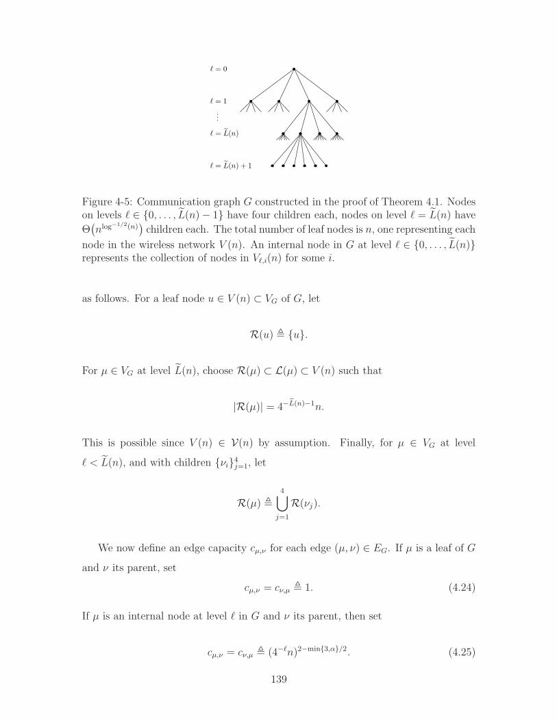
ℓ = 0

ℓ = 1

ℓ = L(n)

ℓ = L(n) + 1

Figure 4-5: Communication graph G constructed in the proof of Theorem 4.1. Nodeson levels ℓ ∈ 0, . . . , L(n) − 1 have four children each, nodes on level ℓ = L(n) have

Θ(nlog−1/2(n)

)children each. The total number of leaf nodes is n, one representing each

node in the wireless network V (n). An internal node in G at level ℓ ∈ 0, . . . , L(n)represents the collection of nodes in Vℓ,i(n) for some i.

as follows. For a leaf node u ∈ V (n) ⊂ VG of G, let

R(u) , u.

For µ ∈ VG at level L(n), choose R(µ) ⊂ L(µ) ⊂ V (n) such that

|R(µ)| = 4−eL(n)−1n.

This is possible since V (n) ∈ V(n) by assumption. Finally, for µ ∈ VG at level

ℓ < L(n), and with children νi4j=1, let

R(µ) ,

4⋃

j=1

R(νj).

We now define an edge capacity cµ,ν for each edge (µ, ν) ∈ EG. If µ is a leaf of G

and ν its parent, set

cµ,ν = cν,µ , 1. (4.24)

If µ is an internal node at level ℓ in G and ν its parent, then set

cµ,ν = cν,µ , (4−ℓn)2−min3,α/2. (4.25)

139

Having chosen edge capacities on G, we can now define the set ΛUC

G (n) ⊂ Rn×n+ of

feasible unicast traffic matrices between leaf nodes ofG. In other words, λUC ∈ ΛUCG (n)

if messages at the leaf nodes of G can be routed to their destinations (which are also

leaf nodes) over G at rates λUC while respecting the capacity constraints on the edges

of G.

We first prove the achievability part of Theorem 4.1. The next lemma shows that

if traffic can be routed over the tree G, then approximately the same traffic can be

transmitted reliably over the wireless network.

Lemma 4.10. Under fast fading, for any α > 2, there exists b(n) ≥ n−o(1) such that

for any V (n) ∈ V(n),

b(n)ΛUC

G (n) ⊂ ΛUC(n).

The same statement holds for slow fading with probability 1 − o(1) as n→ ∞.

Proof. Assume λUC ∈ ΛUC

G , i.e., traffic can be routed between the leaf nodes of G at

a rate λUC, we need to show that n−o(1)λUC ∈ ΛUC (i.e., almost the same flow can be

reliably transmitted over the wireless network). We use the three-layer communication

architecture introduced in Section 4.3 to establish this result.

Recall the three layers of this architecture: the routing, cooperation, and physical

layers. The layers of this communication scheme operate as follows. In the routing

layer, we treat the wireless network as the graph G and route the messages over the

edges of G. The cooperation layer provides this tree abstraction to the routing layer

by distributing and concentrating messages over subsets of the wireless network. The

physical layer implements this distribution and concentration of messages by dealing

with interference and noise.

Consider first the routing layer, and assume that the tree abstraction G can be

implemented in the wireless network with only a n−o(1) factor loss. Since λUC ∈ ΛUCG

by assumption, we then know that the routing layer will be able to reliably transmit

messages at rates n−o(1)λUC. We now show that the tree abstraction can indeed be

implemented in the wireless network.

140

This tree abstraction is provided to the routing layer by the cooperation layer. We

will show that the operation of the cooperation layer satisfies the following invariance

property: If a message is located at a node µ ∈ G in the routing layer, then the same

message is evenly distributed over all nodes in R(µ) in the wireless network. In other

words, all nodes u ∈ R(µ) ⊂ V have access to a distinct part of length 1/|R(µ)| of

the message.

Consider first a leaf node u ∈ V ⊂ VG in G, and assume the routing layer calls

upon the cooperation layer to send a message to its parent ν ∈ VG in G. Note first

that u is also an element of V , and it has access to the entire message to be sent

over G. Since for leaf nodes R(u) = u, this shows that the invariance property is

satisfied at u. The message is split at u into |R(ν)| parts of equal length, and one part

is sent to each node in R(ν) over the wireless network. In other words, we distribute

the message over the wireless network by a factor of |R(ν)|. Hence the invariance

property is also satisfied at µ.

Consider now an internal node µ ∈ VG, and assume the routing layer calls upon

the cooperation layer to send a message to its parent node ν ∈ VG. Note that since

all traffic in G originates at the leaf nodes of G (which are the actual nodes in the

wireless network), a message at µ had to traverse all levels below µ in the tree G. We

assume that the invariance property holds up to level µ in the tree, and show that

it is then also satisfied at level ν. By the induction hypothesis, each node u ∈ R(µ)

has access to a distinct part of length 1/|R(µ)| of the message. Each such node u

splits its message part into four distinct parts of equal length. Node u keeps one part

for itself, and sends the other three parts to nodes in R(ν). Since |R(ν)| = 4|R(µ)|,this can be performed such that each node in R(ν) obtains exactly one message part.

In other words, we distribute the message by a factor four over the wireless network,

and the invariance property is satisfied at ν ∈ VG.

Operation along edges down the tree (i.e., towards the leaf nodes) is similar, but

instead of distributing messages, we now concentrate them over the wireless network.

To route a message from a node µ ∈ VG with internal children νj4j=1 to one of them

(say ν1) in the routing layer, the cooperation layer sends the message parts from each

141

R(νj)4j=2 to a corresponding node in R(ν1) and combines them there. In other

words, we concentrate the message by a factor four over the wireless network.

To route a message to a leaf node u ∈ V ⊂ VG from its parent ν in G in the

routing layer, the cooperation layer sends the corresponding message parts at each

node R(ν) to u over the wireless network. Thus, again we concentrate the message

over the network, but this time by a factor of |R(ν)|. Both these operations along

edges down the tree preserve the invariance property. This shows that the invariance

property is preserved by all operations induced by the routing layer in the cooperation

layer.

Finally, to actually implement this distribution and concentration of messages,

the cooperation layer calls upon the physical layer. Note that at the routing layer, all

edges of the tree can be routed over simultaneously. Therefore, the cooperation layer

can potentially call the physical layer to perform distribution and concentration of

messages over all sets R(µ)µ∈VGsimultaneously. The function of the physical layer

is to schedule all these operations and to deal with the resulting interference as well

as with channel noise.

This scheduling is done as follows. First, the physical layer time shares between

communication up the tree and communication down the tree (i.e., between distri-

bution and concentration of messages). This results in a loss of a factor 1/2 in rate.

The physical layer further time shares between all the L(n) + 1 internal levels of the

tree, resulting in a further 1eL(n)+1

factor loss in rate. Hence, the total rate loss by this

time sharing is1

2(L(n) + 1). (4.26)

Consider now the operations within some level ℓ ∈ 1, . . . , L(n) in the tree (i.e., for

edge (µ, ν) on this level, neither µ nor ν is a leaf node). We show that the rate at

which the physical layer implements the edge (µ, ν) is equal to n−o(1)cµ,ν , i.e., only a

no(1) factor less than the capacity of the edge (µ, ν) in the tree G. Note first that the

distribution or concentration of traffic induced by the cooperation layer to implement

one edge e at level ℓ is restricted to Vℓ−1,i for some i = i(e). We can thus partition

142

the edges at level ℓ into EjG4

j=1 such that the four sets

⋃

e∈EjG

Vℓ−1,i(e)

of nodes are disjoint. Time sharing between these four sets yields an additional loss

of a factor 1/4 in rate. Fix one such value of j, and consider the operations induced

by the cooperation layer in the set corresponding to j. We consider communication

up the tree (i.e., distribution of messages), the analysis for communication down the

tree is similar. For a particular edge (µ, ν) ∈ EjG with ν the parent of µ, each node

u ∈ R(µ) has split its message part into four parts, three of which need to be sent to

other nodes in R(ν). Moreover, this assignment of destination nodes in R(ν) to u is

performed such that no node in R(ν) is destination more than once. In other words,

each node in R(µ) is source exactly three times and each node in R(ν) is destination

at most once. This can be written as three source-destination pairings Πki(µ,ν)3

k=1, on

Vℓ−1,i(µ,ν). Moreover, each such Πki(µ,ν) can be understood as a subset of a permutation

source-destination pairing. We time share between the three values of k (yielding an

additional loss of a factor 1/3 in rate). Now, for each value of k, Lemma 4.9 shows

that by using either hierarchical relaying (for α ∈ (2, 3]) or multi-hop communication

for (α > 3), we can communicate according to Πki(e)e∈Ej

Gat a per-node rate of

n−o(1)(4−ℓ−1n)1−min3,α/2

under fast fading, and with probability 1 − o(1) also under slow fading.3 Since R(µ)

contains 4−ℓ−1n nodes, and accounting for the loss (4.26) for time sharing between

the levels in G and the additional loss of factors 1/4 and 1/3 for time sharing between

j and k, the physical layer implements an edge capacity for e at level ℓ of

1

2(L(n) + 1)· 1

4· 1

3· 4−ℓ−1n · n−o(1)(4−ℓ−1n)1−min3,α/2

3Note that Lemma 4.9 actually shows that all permutation traffic for every value of ℓ can betransmitted with high probability under slow fading. In other words, with high probability all levelsof G can be implemented successfully under slow fading.

143

= n−o(1)(4−ℓn)2−min3,α/2 = n−o(1)ce.

Consider now the operations within level ℓ = L(n) + 1 in the tree (i.e., for edge

(u, ν) on this level, u is a leaf node). We show that the rate at which the physi-

cal layer implements the edge (u, ν) is equal to n−o(1)cu,ν . We again consider only

communication up the tree (i.e., distribution of messages in the cooperation layer),

communication down the tree is performed in a similar manner. The traffic induced

by the cooperation layer at level L(n)+1 is within the sets VeL(n),i for i = 1, . . . , 4eL(n).Consider now communication within one VeL(n),i, and assume without loss of generality

that in the routing layer every node u ∈ VeL(n),i needs to send traffic along the edge

(u, ν). In the physical layer, we need to distribute a 1/|R(ν)| fraction of this traffic

from each node u ∈ VeL(n),i to every node in R(ν) ⊂ VeL(n),i. This can be expressed

as |VeL(n),i| source-destination pairings, and we time share between them. Accounting

for the fact that only 1/|R(ν)| of traffic needs to be sent according to each pairing

and since V ∈ V, this results in a time sharing loss of at most a factor

|R(ν)||VeL(n),i|

≤ 1

16.

Now, using Lemma 4.9, all these source-destination pairings in all subsquares VeL(n),ican be implemented simultaneously at a per node rate of

n−o(1)(4−eLn)1−min3,α/2 ≥ n−o(1)(nlog−1/2(n))−1/2 ≥ n−o(1).

Accounting for the loss (4.26) for time sharing between the levels in G, the additional

factor 1/16 loss for time sharing within each VeL(n),i, the physical layer implements an

edge capacity for e at level ℓ = L(n) + 1 of

1

2(L(n) + 1)· 1

16· n−o(1) = n−o(1) = n−o(1)ce,

under either fast or slow fading.

Together, this shows that the physical and cooperation layers provide the tree

144

abstraction G to the routing layer with edge capacities of only a factor n−o(1) loss.

Hence, if messages can be routed at rates λUC between the leaf nodes of G, then

messages can be reliably transmitted over the wireless network at rates n−o(1)λUC.

Hence

λUC ∈ ΛUC

G ⇒ n−o(1)λUC ∈ ΛUC,

and noting that the n−o(1) factor is uniform in λUC, this shows that

n−o(1)ΛUC

G ⊂ ΛUC.

We have seen that the unicast capacity region ΛUC

G (n) of the graphG under routing

is (appropriately scaled) an inner bound to the unicast capacity region ΛUC(n) of the

wireless network. The next lemma shows that ΛUCG (n) is equal to the approximate

unicast capacity region ΛUC1 (n) of the wireless network as defined in (4.2). Combining

Lemmas 4.5, 4.10, and 4.11 below, yields that with high probability

n−o(1)ΛUC(n) ⊂ n−o(1)ΛUC

G (n) ⊂ ΛUC(n),

proving the achievability part of Theorem 4.1.

Lemma 4.11. For any α > 2 and any V (n) ∈ V(n),

ΛUC

1 (n) = ΛUC

G (n).

Proof. We first relate the total traffic across an edge e in the graph G to the total

traffic across a cut Vℓ,i for some ℓ and i.

Consider an edge e = (µ, ν) ∈ EG, and assume first that e connects a node at

level ℓ+ 1 and ℓ in the tree with ℓ < L(n). We slight abuse of notation, set

ce , cµ,ν .

145

Note first that by (4.25) we have

ce = (4−ℓn)2−min3,α/2. (4.27)

Moreover, since G is a tree, removing the edge e from EG separates the tree into two

connected components, say S1, S2 ⊂ VG. Consider now the leaf nodes in S1. By the

construction of the tree structure of G, these leaf nodes are either equal to Vℓ,i or V cℓ,i

for some i ∈ 1, . . . , 4ℓ. Assume without loss of generality that they are equal to Vℓ,i.

Then V cℓ,i are the leaf nodes in S2. Now since traffic is only assumed to be between

leaf nodes of G, the total traffic demand between S1 and S2 is equal to

∑

u∈Vℓ,i

∑

w∈V cℓ,i

(λUC

u,w + λUC

w,u). (4.28)

By the tree structure of G, all this traffic has to be routed over edge e.

Consider now an edge e connecting a node at level L(n) + 1 and L(n), i.e., a leaf

node u to its parent ν. Then, by (4.24),

ce = 1, (4.29)

and the total traffic crossing the edge e is equal to

∑

w 6=u

(λUC

u,w + λUC

w,u). (4.30)

We now show that

ΛUC

1 ⊂ ΛUC

G . (4.31)

Assume λUC ∈ ΛUC1 , then

∑

u∈Vℓ,i

∑

w∈V cℓ,i

(λUC

u,w + λUC

w,u) ≤ (4−ℓn)2−min3,α

146

for all ℓ ∈ 1, . . . , L(n), i ∈ 1, . . . , 4ℓ, and

∑

w 6=u

(λUC

u,w + λUC

w,u) ≤ 1

for all u ∈ V . By (4.27), (4.28), (4.29), (4.30), this implies that the traffic demand

across each edge e of the graph G is less than its capacity ce. Since G is a tree, this

implies that λUC can be routed over G, i.e., λUC ∈ ΛUC

G . This proves (4.31).

We now show that

ΛUC

G ⊂ ΛUC

1 . (4.32)

Assume λUC ∈ ΛUCG . This implies λUC can be routed over G, and hence the total

flow across each edge is less than the capacity of that edge. By (4.27), (4.28), (4.29),

(4.30), this implies λUC ∈ ΛUC1 , from which (4.32) follows.

We now turn to the converse part of Theorem 4.1. The next lemma shows that

ΛUC2 (n) (appropriately scaled) is an outer bound to the unicast capacity region ΛUC(n)

of the wireless network. Combined with Lemma 4.5, this shows that with high prob-

ability

ΛUC(n) ⊂ O(log6(n))ΛUC

2 (n),

proving the converse part of Theorem 4.1.

Lemma 4.12. Under either fast or slow fading, for any α > 2, there exists b(n) =

O(log6(n)) such that for any V (n) ∈ V(n),

ΛUC(n) ⊂ b(n)ΛUC(n).

Proof. Assume λUC ∈ ΛUC. By Lemma 4.7, we have for any ℓ ∈ 1, . . . , L(n) and

i ∈ 1, . . . , 4ℓ,∑

u∈Vℓ,i

∑

v∈V cℓ,i

λUC

u,v ≤ K log6(n)(4−ℓn)2−min3,α/2, (4.33)

for some constant K not depending on λUC. Moreover, Lemma 4.6 shows that for all

147

u ∈ V∑

v 6=u

(λUC

u,v + λUC

v,u) ≤ 2K log(n). (4.34)

Combining (4.33) and (4.34) proves that there exists b(n) = O(log6(n)) such that

λUC ∈ ΛUC implies λUC ∈ b(n)ΛUC2 , proving the lemma.

4.6 Proof of Theorem 4.2

Assume λUC ∈ ΛUC. By Lemmas 4.7 and 4.8, we have for any ℓ ∈ 1, . . . , L(n),i ∈ 1, . . . , 4ℓ, and α > 5,

max∑

u∈Vℓ,i

∑v∈V c

ℓ,iλUC

u,v,∑

u∈V cℓ,i

∑v∈Vℓ,i

λUCu,v,≤ K log6(n)(4−ℓn)2−min3,α/2,

for some constant K not depending on λUC. Hence

∑

u∈Vℓ,i

∑

v∈V cℓ,i

(λUC

u,v,+λUC

v,u) ≤ 2K log6(n)(4−ℓn)2−min3,α/2.

Combined with the outer bound in Theorem 4.1, this shows that there exists b(n) =

O(log6(n)) such that for α > 5, λUC ∈ ΛUC implies λUC ∈ b(n)ΛUC1 , proving Theorem

4.2.

4.7 Discussion

We discuss several aspects and extensions of the three-layer architecture introduced

in Section 4.3 and used to show achievability in Theorem 4.1. In Section 4.7.1,

we comment on the various tree structures used in the three-layer architecture. In

Section 4.7.2, we show that for certain values of α the bounds in Theorem 4.1 can be

significantly sharpened. In Section 4.7.3, we point out how the results discussed so

far can be used to obtain the scaling of the unicast capacity region of dense networks

(where n nodes are randomly placed on a square of unit area). Section 4.7.4 contains

design guidelines that can be obtained from the scaling results for the unicast capacity

148

region presented in this chapter.

4.7.1 Tree Structures

There are two distinct tree structures that are used in the construction of the three-

layer communication scheme proposed in this chapter — one explicit and one implicit.

These two tree structures appear in different layers of the communication scheme and

serve different purposes.

The first (explicit) tree structure is given by the tree G utilized in the routing layer

and implemented in the cooperation layer. The main purpose of this tree structure

is to perform localized load balancing. In fact, the distribution and concentration of

traffic is used to avoid unnecessary bottlenecks. Note that the tree G is used by the

scheme for any value of α.

The second (implicit) tree structure occurs in the physical layer. This tree struc-

ture appears only for values of α ∈ (2, 3], when the physical layer operates using the

hierarchical relaying scheme (see Chapter 3). It is this hierarchical structure of this

scheme that can equivalently be understood as a tree. The purpose of this second tree

structure is to enable multiple antenna communication, i.e., to perform cooperative

communication.

4.7.2 Second-Order Asymptotics

The scaling result in Theorems 4.1 and 4.2 are up to a factor n±o(1) and hence preserve

information at scale nβ for constant β (see also the discussion in Section 4.1.2). Here

we take a closer look at the behavior of this n±o(1) factor, and show that in certain

situations it can be significantly sharpened.

Note first that the outer bound in Theorems 4.1 and 4.2 hold up to a factor

log6(n), i.e., poly-logarithmic in n. However, the inner bound holds only up to the

aforementioned n−o(1) factor. A closer look at the proof of the theorems reveals that

149

the precise inner bound is of order

n−O(

log−1/4(n)),

and with a more careful analysis (see Chapter 3 for the details), this can be sharpened

to essentially

n−O(

log−1/2(n)).

The exponent log−1/2(n) in the inner bound has two causes. The first is the use

of hierarchical relaying (for α ∈ (2, 3]). The second is the operation of the physical

layer at level L(n)+ 1 of the tree (i.e., to implement communication between the leaf

nodes of G and their parents). Indeed at that level, we are operating on a square of

area

4−eL(n)n = nlog1/2(n),

and the loss is essentially inversely proportional to that area. Now, the reason why

L(n) cannot be chosen to be larger (to make this loss smaller), is because hierarchical

relaying requires a certain amount of regularity in the node placement, which can

only be guaranteed for large enough areas.

This suggests that for the α > 3 regime, where multi-hop communication is used

at the physical layer instead of hierarchical relaying, we might be able to significantly

improve the inner bound. To this end, we have to choose more levels in the tree G,

such that at the last level before the tree nodes, we are operating on a square that

has an area of order log(n). Changing the three-layer architecture in this manner, for

α > 3 the inner bound can be improved to be poly-logarithmic in n as well. Combined

with the poly-logarithmic outer bound, this yields a poly-logarithmic approximation

for n2 − n out of n2 total dimensions of the unicast capacity region ΛUC(n) for α ∈(3, 5], and a poly-logarithmic approximation for the entire unicast capacity region

ΛUC(n) for α > 5.

150

4.7.3 Dense Networks

So far, we have only discussed extended networks, i.e., n nodes are located on a square

of area n. We now briefly sketch how these results can be recast for dense networks,

in which n nodes are located on a square of unit area. It suffices to notice that by

rescaling power by a factor n−α/2, a dense network can essentially be transformed

into an equivalent extended network with path-loss exponent α (see also [38]). Hence

the scaling of the unicast capacity region for dense networks can be obtained from

the scaling result for extended networks by taking a limit as α → 2.

The resulting approximate unicast capacity region ΛUC1 (n) has a particularly sim-

ple shape in this limit. In fact, the only constraints in (4.2) that can be tight are at

level ℓ = log(n). This results in the following approximate unicast capacity region for

dense networks:

ΛUC

1 (n) ,λUC ∈ R

n×n+ :

∑

v 6=u

(λUC

u,v + λUC

v,u) ≤ 1, ∀ u ∈ V (n),

and we obtain that for dense networks, for any α > 2,

n−o(1)ΛUC

1 (n) ⊂ ΛUC(n) ⊂ O(log6(n))ΛUC

1 (n).

Note that, in contrast to the extended case, this results in an approximate character-

ization of the entire unicast region for all α > 2.

4.7.4 Design Guidelines

The results presented in this chapter suggest the following design guidelines for the

construction and operation of large wireless networks. First, it shows that load balanc-

ing is crucial for optimal operation. This is implemented in the proposed three-layer

architecture by spreading traffic over clusters of neighbors, but could be achieved in

other ways as well. A communication protocol not using such load balancing could

create bottlenecks that prevent it from operating optimally. It is worth pointing out

that in the case of random source-destination pairing with uniform rate no such load

151

balancing is necessary since the traffic demand itself is already balanced.

Second, the load balancing has to be done in a localized manner. In the three-layer

architecture, this is achieved by choosing the cluster over which the load balancing is

performed to be those nodes that are in the same smallest square Vℓ,i(n) that contains

both the source and its destination. Again, other ways to perform this load balancing

are possible, however for optimal operation this load balancing must have the same

localized structure.

Finally, recall that for random node placement and random source-destination

pairing with uniform rate, hierarchical cooperation is order optimal for α ∈ (2, 3],

and multi-hop communication is order optimal for α > 3. The same threshold phe-

nomenon occurs also for random node placement with heterogeneous traffic. In the

three-layer architecture, this is visible in the physical layer, which uses hierarchical

relaying for α ∈ (2, 3] and multi-hop communication for α > 3. In other words,

for optimal transmission of heterogeneous traffic over randomly placed nodes, global

cooperation is necessary for small path-loss exponents, and local cooperation is suf-

ficient for large path-loss exponents. Note that the assumption of randomly placed

nodes is crucial for this conclusion to be valid, as was discussed in detail in Section 3.

4.8 Chapter Summary

In this chapter, we have obtained information-theoretic inner and outer bounds on

the n2-dimensional unicast capacity region of a wireless network with n randomly

placed nodes and assuming a Gaussian fading channel model. These bounds are

tight (in the scaling sense) along n2 − n of the total n2 dimensions for α ∈ (2, 5]

(corresponding to balanced traffic), and along all n2 dimensions for α > 5. This

approximate characterization is in terms of 2n weighted cuts, which are based on the

geometry of the locations of the source nodes and their destination nodes and on the

traffic demands between them, and thus can be readily evaluated.

This characterization is obtained by establishing that, for balanced traffic or for

α > 5, the unicast capacity region of a capacitated tree graph under routing has the

152

same scaling as the unicast capacity region of the original wireless network. The leaf

nodes of this tree graph correspond to the nodes in the wireless network, and internal

nodes of the tree graph correspond to hierarchically growing sets of nodes.

This equivalence suggests a three-layer communication architecture for achieving

the entire unicast capacity region (in the scaling sense). The top or routing layer

establishes paths from each of the source nodes to its destination over the tree graph.

The middle or cooperation layer provides this tree abstraction to the routing layer

by distributing the traffic among the corresponding subset of nodes as a message

travels up the tree graph, and by concentrating the traffic on to the corresponding

subset of nodes as the message travels down the tree. The bottom or physical layer

implements this distribution and concentration of traffic over the wireless network.

The implementation of this distribution and concentration of traffic depends on the

path-loss exponent: For low path-loss exponent (α ∈ (2, 3]), hierarchical relaying is

used, while for high path-loss exponent (α > 3), multi-hop communication is used.

153

154

Chapter 5

Service Heterogeneity: Multicast

In this chapter, we analyze the scaling of the n × 2n-dimensional multicast capacity

region ΛMC(n) of a wireless network of n randomly placed nodes under a Gaussian

fading channel model.

We first present an inner and an outer bound to the n× 2n-dimensional multicast

capacity region. We show that the two bounds coincide (up to scaling) along n2n −n dimensions (corresponding to balanced traffic) for α ∈ (2, 5] and along all n2n

dimensions for α > 5. We show that, as the unicast capacity region, the multicast

capacity region can be approximated by a polytope with less than 2n faces, each

corresponding to a distinct cut (i.e., a subset of nodes) in the wireless network. Again,

as in the unicast case, only 2n out of 2n possible cuts in the wireless network are

asymptotically relevant.

Second, we show how the three-layer communication architecture introduced in

Chapter 4 can be adapted for the transmission of multicast traffic. Recall the three

layers of this scheme: The routing layer, the cooperation layer, and the physical layer.

We show that only the routing layer needs to be changed to accommodate multicast

traffic. The other two layers are unaffected. The approximate optimality of this

three-layer architecture implies that a separation based approach, in which routing is

performed independently of the physical layer, is order-optimal for balanced multicast

traffic or for α > 5, and hence techniques such as network coding are not necessary

for order-optimal transmission of multicast traffic in wireless networks.

155

5.0.1 Organization

The remainder of this chapter is organized as follows. Section 5.1 presents the main

results of this chapter. In Section 5.2, we analyze various examples scenarios with

heterogeneous multicast traffic patterns for which no scaling results were previously

known. Section 5.3 provides a high-level description of the modifications to the three-

layer architecture required for multicast traffic. Section 5.4 contains the proofs of

the main results. Finally, Sections 5.5 and 5.6 contain discussions and concluding

remarks.

5.1 Main Results

This section contains the main results of this chapter. In Section 5.1.1, we provide

inner and outer bounds on the multicast capacity region ΛMC(n) and conditions for

these bounds to be tight in the scaling sense. In Section 5.1.2, we discuss implications

of these results on the behavior of the multicast capacity region for large values of n.

We consider computational aspects in Section 5.1.3.

5.1.1 Multicast Capacity Region

Recall the definition of L(n) in (4.1) and of the subsets Vℓ,i(n)4ℓ

i=1 of V (n) at level

ℓ in Section 4.1.1. Define

ΛMC

1 (n) ,λMC ∈ R

n×2n

+ :

∑

u∈Vℓ,i(n)

∑

W⊂V (n):W∩V c

ℓ,i(n)6=∅

λMC

u,W +∑

u∈V cℓ,i(n)

∑

W⊂V (n):W∩Vℓ,i(n)6=∅

λMC

u,W ≤ (4−ℓn)2−min3,α/2

∀ℓ ∈ 1, . . . , L(n), i ∈ 1, . . . 4ℓ,∑

W⊂V (n):W\u6=∅

λMC

u,W +∑

u 6=u

∑

W⊂V (n):u∈W

λMC

u,W ≤ 1

∀u ∈ V (n),

(5.1)

156

and

ΛMC

2 (n) ,λMC ∈ R

n×2n

+ :

∑

u∈Vℓ,i(n)

∑

W⊂V (n):W∩V c

ℓ,i(n)6=∅

λMC

u,W ≤ (4−ℓn)2−min3,α/2

∀ℓ ∈ 1, . . . , L(n), i ∈ 1, . . . 4ℓ,∑

W⊂V (n):W\u6=∅

λMC

u,W +∑

u 6=u

∑

W⊂V (n):u∈W

λMC

u,W ≤ 1

∀u ∈ V (n).

The definitions of ΛMC1 (n) and ΛMC

2 (n) are similar to those of ΛUC1 (n) and ΛUC

2 (n)

in Chapter 4. ΛMC1 (n) and ΛMC

2 (n) are the collection of all multicast traffic matrices

λMC such that for various cuts S ⊂ V (n) in the network, the total traffic demand (in

either one or both directions)

∑

u∈S

∑

W⊂V (n):W∩Sc 6=∅

λMC

u,W

∑

u∈S

∑

W⊂V (n):W∩Sc 6=∅

λMC

u,W +∑

u∈Sc

∑

W⊂V (n):W∩S 6=∅

λMC

u,W

across the cut S is not too big. Note that, unlike in the definitions of ΛUC1 (n) and

ΛUC2 (n), we count λu,W as crossing the cut S (in the outgoing direction, say) if u ∈ S

and W ∩Sc 6= ∅, i.e., if there is at least one node w in the multicast destination group

W that lies outside S. The number of such cuts S we need to consider is at most 2n,

as in the unicast case.

The next theorem shows that ΛMC1 (n) is an approximate (in the scaling sense)

inner bound and ΛMC2 (n) is an approximate outer bound to the multicast capacity

region ΛMC(n) of the wireless network.

157

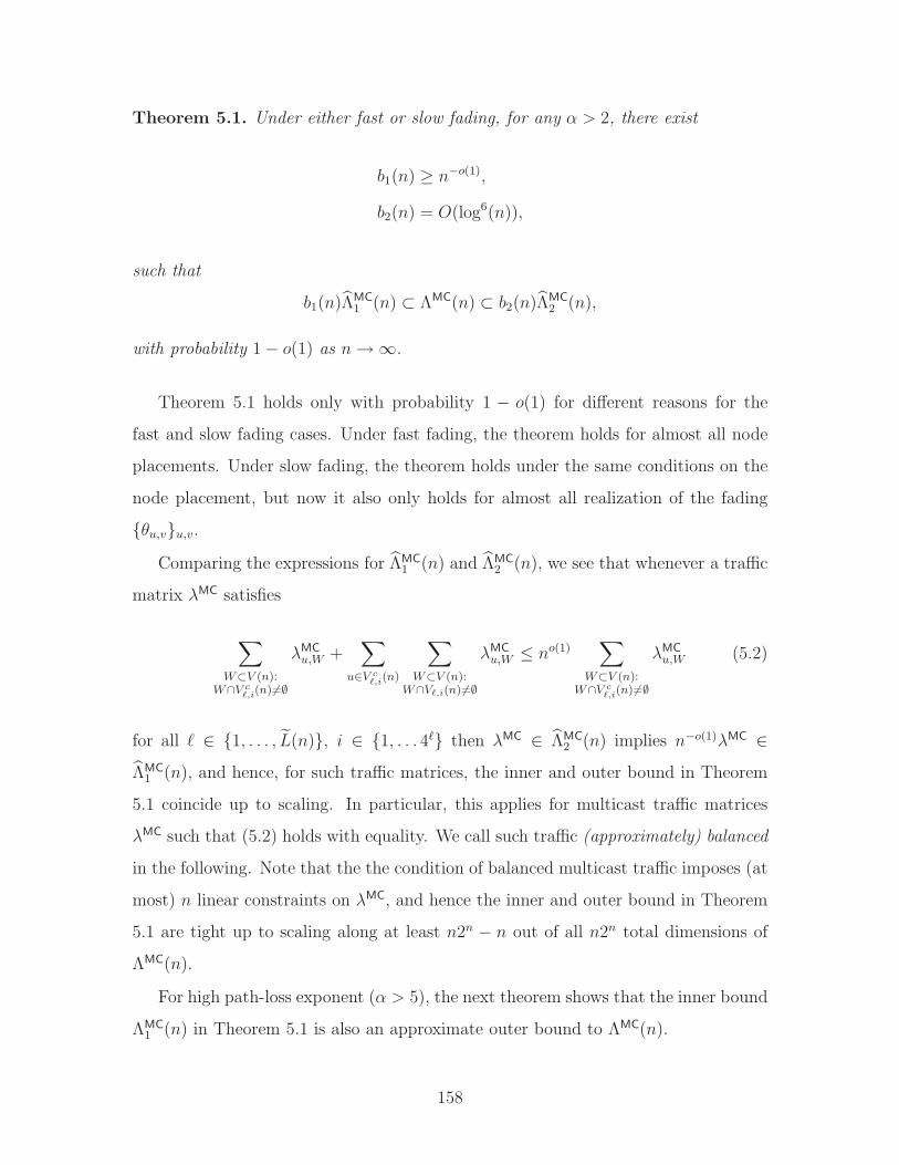
Theorem 5.1. Under either fast or slow fading, for any α > 2, there exist

b1(n) ≥ n−o(1),

b2(n) = O(log6(n)),

such that

b1(n)ΛMC

1 (n) ⊂ ΛMC(n) ⊂ b2(n)ΛMC

2 (n),

with probability 1 − o(1) as n→ ∞.

Theorem 5.1 holds only with probability 1 − o(1) for different reasons for the

fast and slow fading cases. Under fast fading, the theorem holds for almost all node

placements. Under slow fading, the theorem holds under the same conditions on the

node placement, but now it also only holds for almost all realization of the fading

θu,vu,v.

Comparing the expressions for ΛMC1 (n) and ΛMC

2 (n), we see that whenever a traffic

matrix λMC satisfies

∑

W⊂V (n):W∩V c

ℓ,i(n)6=∅

λMC

u,W +∑

u∈V cℓ,i(n)

∑

W⊂V (n):W∩Vℓ,i(n)6=∅

λMC

u,W ≤ no(1)∑

W⊂V (n):W∩V c

ℓ,i(n)6=∅

λMC

u,W (5.2)

for all ℓ ∈ 1, . . . , L(n), i ∈ 1, . . . 4ℓ then λMC ∈ ΛMC2 (n) implies n−o(1)λMC ∈

ΛMC1 (n), and hence, for such traffic matrices, the inner and outer bound in Theorem

5.1 coincide up to scaling. In particular, this applies for multicast traffic matrices

λMC such that (5.2) holds with equality. We call such traffic (approximately) balanced

in the following. Note that the the condition of balanced multicast traffic imposes (at

most) n linear constraints on λMC, and hence the inner and outer bound in Theorem

5.1 are tight up to scaling along at least n2n − n out of all n2n total dimensions of

ΛMC(n).

For high path-loss exponent (α > 5), the next theorem shows that the inner bound

ΛMC1 (n) in Theorem 5.1 is also an approximate outer bound to ΛMC(n).

158

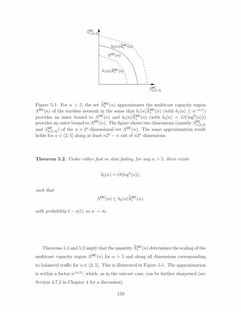
λMC

2,1,3

ΛMC(n)

b1(n)ΛMC1 (n)

b3(n)ΛMC1 (n)

λMC

1,2,3

Figure 5-1: For α > 5, the set ΛMC1 (n) approximates the multicast capacity region

ΛMC(n) of the wireless network in the sense that b1(n)ΛMC1 (n) (with b1(n) ≥ n−o(1))

provides an inner bound to ΛMC(n) and b3(n)ΛMC1 (n) (with b3(n) = O

(log6(n)

))

provides an outer bound to ΛMC(n). The figure shows two dimensions (namely λMC

1,2,3and λMC

2,1,3) of the n × 2n-dimensional set ΛMC(n). The same approximation result

holds for α ∈ (2, 5] along at least n2n − n out of n2n dimensions.

Theorem 5.2. Under either fast or slow fading, for any α > 5, there exists

b3(n) = O(log6(n)),

such that

ΛMC(n) ⊂ b3(n)ΛMC

1 (n),

with probability 1 − o(1) as n→ ∞.

Theorems 5.1 and 5.2 imply that the quantity ΛMC1 (n) determines the scaling of the

multicast capacity region ΛMC(n) for α > 5 and along all dimensions corresponding

to balanced traffic for α ∈ (2, 5]. This is illustrated in Figure 5-1. The approximation

is within a factor n±o(1), which, as in the unicast case, can be further sharpened (see

Section 4.7.2 in Chapter 4 for a discussion).

159

5.1.2 Implications of Theorems 5.1 and 5.2

As in the unicast case, Theorems 5.1 and 5.2 can be applied in two ways. First,

the theorem can be used to analyze the asymptotic achievability of a sequence of

multicast traffic matrices. Let λMC(n)n≥1 be such a sequence of multicast traffic

matrices with λMC(n) ∈ Rn×2n

+ . Define

ρ∗λMC(n) , supρ : ρλMC(n) ∈ ΛMC(n),

ρ∗λMC(n) , supρ : ρλMC(n) ∈ ΛMC(n),

in analogy to the unicast case. Theorems 5.1 and 5.2 state that if either α > 5 or all

λMC(n) are balanced then1

limn→∞

log(ρ∗λMC(n))

log(n)= lim

n→∞

log(ρ∗λMC(n))

log(n).

Several applications of this approach are explored in Section 5.2.

Second, Theorems 5.1 and 5.2 provide information about the shape of the multicast

capacity region ΛMC(n). As in the unicast case, the boundary points of ΛMC(n) vary

at least from n−min3,α/2+o(1) to n−o(1), and this variation on exponential scale is

preserved by ΛMC1 (n) and ΛMC

2 (n). See also Section 4.1.2 for more details.

5.1.3 Computational Aspects

In this section, we show that ΛMC1 (n) can be efficiently described. By Theorems 5.1

and 5.2 this yields a computationally efficient approximate description of the entire

multicast capacity region ΛMC(n) for α > 5 and of n2n − n of its n2n dimensions for

α ∈ (2, 5].

The multicast capacity region ΛMC(n) is a n×2n-dimensional set, i.e., the number

of dimensions is exponentially large in n. Nevertheless, its approximation ΛMC1 (n)

can (as in the unicast case) be computed by evaluating at most 2n cuts. This yields

1We again assume that the limits exist, otherwise the same statement holds for lim sup andlim inf.

160

a very compact approximate representation of the multicast capacity region ΛMC(n)

(i.e., we represent a region of exponential size in n as an intersection of only linearly

many halfspaces — one halfspace corresponding to each cut). Moreover, it implies

that membership λMC ∈ ΛMC1 (n) can be computed efficiently. More precisely, evalu-

ating each of the Θ(n) cuts takes at most |(u,W ) : λMCu,W > 0| operations. Thus

membership λMC ∈ ΛMC1 (n) can be tested in at most Θ(n) times more operations than

required to just read the problem parameters. In other words, we have a linear time

(in the length of the input) algorithm for testing membership of a multicast traffic

matrix λMC in ΛMC1 (n), and hence for α > 5 or balanced λMC also for approximate

testing of membership in ΛMC(n). However, this algorithm is not necessarily linear

time in n since reading just the input λMC ∈ Rn×2n

+ itself might take exponential time

in n.

5.2 Example Scenarios

Here we consider several multicast scenarios. The first two examples consider broad-

cast traffic. The third and fourth examples consider proper multicast traffic (i.e., only

a subset of nodes acts as destinations).

Example 5.1. Broadcast from one source

Assume we have only one source (say u0 ∈ V (n)) that wants to broadcast the

same message to all other nodes. In other words, we consider the multicast traffic

matrix

λMC

u,W =

ρ(n) if u = u0 and W = V (n),

0 else,

for some ρ(n) > 0. Applying Theorem 5.1 yields that ρ∗(n), the largest achievable

ρ(n), satisfies

ρ∗(n) = n±o(1)

with probability 1 − o(1) as n → ∞. This implies that the source can broadcast its

information at essentially constant rate independent of n to all nodes in the network.

161

Hence, broadcasting information from one source to all nodes in the network is (at

least asymptotically) no harder than transmitting information from one source to its

destination. ♦

Example 5.2. Broadcast from many sources

Consider a scenario with nβ sources, u1, . . . , unβ), for some 0 ≤ β ≤ 1, each

broadcasting an independent message to all other nodes at the same rate. In other

words, we have a multicast traffic matrix of the form

λMC

u,W =

ρ(n) if u = ui for some i and W = V (n),

0 else,

for some ρ(n) > 0. Applying Theorem 5.1 yields that ρ∗(n), the largest achievable

ρ(n), satisfies

ρ∗(n) = n−β±o(1),

with probability 1 − o(1) as n→ ∞. ♦

Example 5.3. Multicast from many sources

Assume each node generates independent multicast traffic for a set of nβ destina-

tions. All these sources and their destinations are chosen independently and uniformly

at random from V (n). Let u1, . . . , un be the source nodes and W1, . . . ,Wn with

|Wi| = nβ the corresponding multicast nodes. Then the multicast traffic matrix λMC

is of the form

λMC

u,W =

ρ(n) if u = ui,W = Wi for some i,

0 else,

(5.3)

for some ρ(n) > 0. This traffic matrix is approximately balanced with high probabil-

ity, and hence applying Theorem 5.1 yields that ρ∗(n) satisfies

ρ∗(n) = minn±o(1), n(1−β)(2−α/2)−1±o(1)

(5.4)

162

with probability 1 − o(1) as n→ ∞, and with

α , min3, α.

Note that for β2 = 0, we recover the result for unicast traffic with random source-

destination pairing and uniform rate. ♦

Example 5.4. Localized multicast from many sources

Consider the setup of Example 5.3 above, except now each source picks nβ1 des-

tinations uniformly at random from among nodes within a distance of nβ22 , where

β2 > β1. In other words, each source node performs localized multicast. Again, let

u1, . . . , un denote the source nodes and W1, . . . ,Wn, with |Wi| = nβ1 , denote the

corresponding destination nodes, where now rui,v ≤ nβ22 , for each v ∈Wi. The multi-

cast traffic matrix λMC is of the form (5.3). This traffic matrix is again approximately

balanced with high probability, and an application of Theorem 5.1 shows that ρ∗(n)

satisfies

ρ∗(n) = minn±o(1), n(β2−β1)(2−α/2)−β2±o(1)

with probability 1− o(1) as n→ ∞. Note that setting β2 = 1, i.e., each source picks

its destinations uniformly over the entire region A(n), yields the same scaling of ρ∗(n)

as in Example 5.3. Similarly, for β1 = 0, and β2 = β, we recover the unicast scenario

with K = 1 in Example 4.1. ♦

5.3 Communication Scheme for Multicast Traffic

Here we show that the same communication scheme presented in Section 4.3 for

general unicast traffic can also be used to transmit general multicast traffic. It is the

tree structure of the scheme that is critically exploited in the proof of Theorem 5.1

to obtain an approximation of the multicast capacity region ΛMC(n).

We will use the same three-layer architecture as for unicast traffic presented in

Section 4.3. Note that for this, we only need to modify the operation of the top or

163

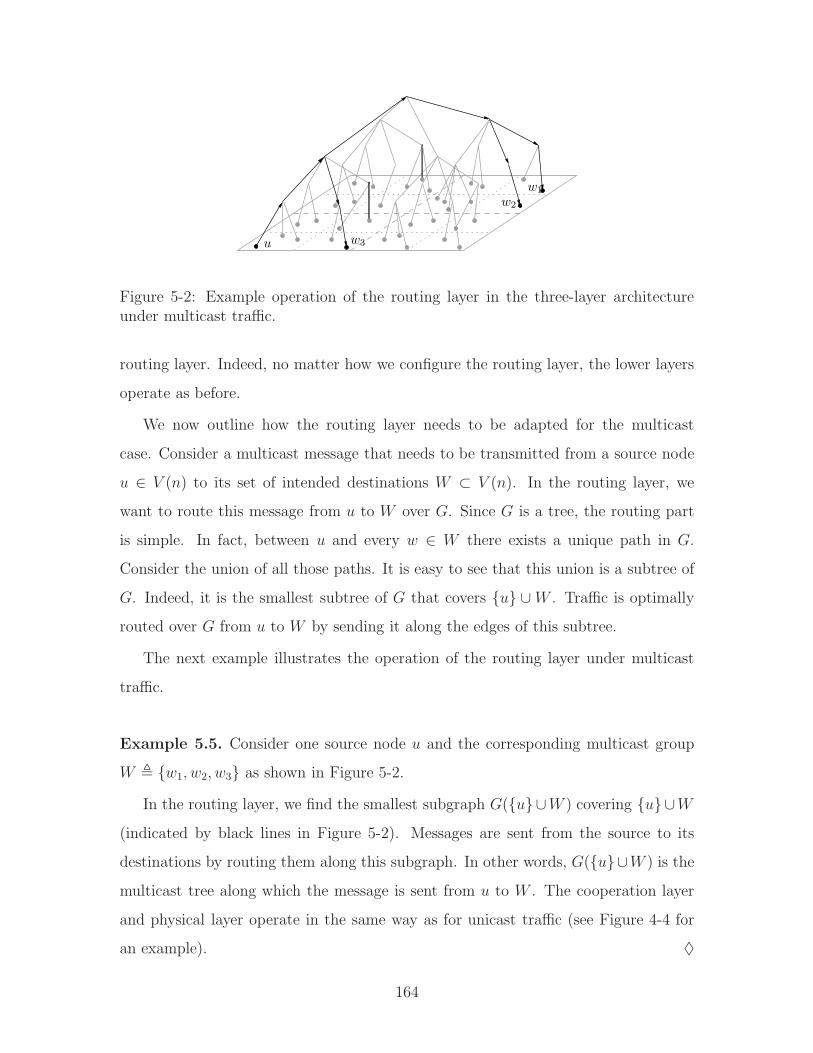
u w3

w2

w1

Figure 5-2: Example operation of the routing layer in the three-layer architectureunder multicast traffic.

routing layer. Indeed, no matter how we configure the routing layer, the lower layers

operate as before.

We now outline how the routing layer needs to be adapted for the multicast

case. Consider a multicast message that needs to be transmitted from a source node

u ∈ V (n) to its set of intended destinations W ⊂ V (n). In the routing layer, we

want to route this message from u to W over G. Since G is a tree, the routing part

is simple. In fact, between u and every w ∈ W there exists a unique path in G.

Consider the union of all those paths. It is easy to see that this union is a subtree of

G. Indeed, it is the smallest subtree of G that covers u ∪W . Traffic is optimally

routed over G from u to W by sending it along the edges of this subtree.

The next example illustrates the operation of the routing layer under multicast

traffic.

Example 5.5. Consider one source node u and the corresponding multicast group

W , w1, w2, w3 as shown in Figure 5-2.

In the routing layer, we find the smallest subgraph G(u∪W ) covering u∪W(indicated by black lines in Figure 5-2). Messages are sent from the source to its

destinations by routing them along this subgraph. In other words, G(u∪W ) is the

multicast tree along which the message is sent from u to W . The cooperation layer

and physical layer operate in the same way as for unicast traffic (see Figure 4-4 for

an example). ♦

164

5.4 Proofs

This Section contains the proofs of Theorem 5.1 (in Section 5.4.1) and of Theorem

5.2 (in Section 5.4.2).

5.4.1 Proof of Theorem 5.1

The proof of Theorem 5.1 relies on linking the multicast capacity region to the unicast

capacity region. We say that a unicast traffic matrix λUC is compatible with a multicast

traffic matrix λMC if there exists a mapping f : V (n) × 2V (n) → V (n) such that

f(u,W ) ∈W , for all (u,W ), and

λUC

u,v =∑

W⊂V (n):f(u,W )=v

λMC

u,W

for all (u, v). In words, λMC is compatible with λUC if we can create the unicast traffic

matrix λUC from λMC by simply discarding the traffic for the pair (u,W ) at all the

nodes W \f(u,W ). Let Γ(λMC) be the set of all unicast traffic matrices compatible

with the multicast traffic matrix λMC. We extend the definition of Γ to sets of traffic

matrices as follows:

Γ(ΛMC(n)

),

⋃

λMC∈ΛMC(n)

Γ(λMC),

Γ−1(ΛUC(n)

),λMC : Γ(λMC) ⊂ ΛUC(n)

.

In words, Γ(ΛMC(n)

)is the collection of all unicast traffic matrices that are compatible

with a multicast traffic in ΛMC(n), and Γ−1(ΛUC(n)

)is the collection of all multicast

traffic matrices that have all their compatible unicast traffic matrices in ΛUC(n).

We start with some auxiliary lemmas for the outer bound in Theorem 5.1.

Lemma 5.3. Under either fast or slow fading, for any α > 2,

ΛMC(n) ⊂ Γ−1(ΛUC(n)

).

165

Proof. It is clear that if λMC ∈ ΛMC then λUC ∈ ΛUC for any λUC ∈ Γ(λMC). Indeed,

we can reliably transmit at rate λUC by using the communication scheme for λMC and

simply discarding the messages delivered by this scheme at all but one node in each

multicast destination group. Thus λMC ∈ ΛMC implies Γ(λMC) ⊂ ΛUC, and therefore

Γ(ΛMC

)=

⋃

λMC∈ΛMC

Γ(λMC

)⊂ ΛUC,

or, equivalently,

ΛMC ⊂ Γ−1(ΛUC

),

proving the lemma.

We now prove several auxiliary results for the inner bound in Theorem 5.1. Con-

sider again the tree graph G = (VG, EG) with leaf nodes V (n) ⊂ VG constructed in

Section 4.5. As before, we consider traffic between leaf nodes of G. In particular,

any multicast traffic matrix λMC ∈ Rn×2n

+ for the wireless network is also a multicast

traffic matrix for the graph G. Denote by ΛMCG (n) ⊂ R

n×2n

+ the set of feasible (under

routing) multicast traffic matrices between leaf nodes of G.

The next lemma shows that if multicast traffic can be routed over G then ap-

proximately the same multicast traffic can be transmitted reliably over the wireless

network. Before we state that lemma, recall the definition of the set V(n) of node

placements V (n) that satisfy certain regularity conditions as defined in Section 4.4.1.

Lemma 5.4. Under fast fading, for any α > 2, there exists b(n) ≥ n−o(1) such that

for all V (n) ∈ V(n),

b(n)ΛMC

G (n) ⊂ ΛMC(n).

The same statement holds under slow fading with probability 1 − o(1) as n→ ∞.

Proof. The proof follows using the same construction as in Lemma 4.10.

We now show that since G is a tree graph, the multicast capacity region ΛMC

G (n)

can be described through the unicast capacity region ΛUCG (n) of G. The fact that G

166

is a tree is critical for this result to hold.

Lemma 5.5. For any α > 2,

Γ−1(ΛUC

G (n))⊂ ΛMC

G (n).

Proof. Assume that λMC /∈ ΛMC

G . Since G is a tree, there is only one way to route

multicast traffic from u to W , namely along the subtree G(u ∪ W ) induced by

u ∪W (i.e., the smallest subtree of G that covers u ∪W ). Hence for any edge

e ∈ EG, the traffic dλMC(e) that needs to be routed over e is equal to

dλMC(e) =∑

u∈V,W⊂V :e∈EG(u∪W )

λMC

u,W .

Now, since λMC /∈ ΛMCG , there exists e ∈ EG such that

dλMC(e) > ce.

But then, by definition of dλMC(e), there exists a function f : V × 2V → V with

f(u,W ) ∈W for all (u,W ), and such that

dλUC

f (λMC)(e) = dλMC(e) > ce,

where λUC

f (λMC) is the unicast traffic matrix resulting from applying f to the multicast

traffic matrix λMC. Thus λUC

f (λMC) /∈ ΛUCG .

We have shown that if λMC /∈ ΛMCG then there exists λUC ∈ Γ(λMC) such that λUC /∈

ΛUC

G . In other words, Γ(λMC) is not a subset of ΛUC

G , and therefore λMC /∈ Γ−1(ΛUC

G

).

Hence λMC /∈ ΛMCG implies λMC /∈ Γ−1

(ΛUC

G ), and thus

Γ−1(ΛUC

G

)⊂ ΛMC

G .

167

We are now ready for the proof of Theorem 5.1. Note that

Γ(λMC) ⊂ ΛUC

j (n) ⇔ λMC ∈ ΛMC

j (n),

and hence

Γ−1(ΛUC

j (n))

= ΛMC

j (n), (5.5)

for j ∈ 1, 2.

For the inner bound in Theorem 4.1, we have for V ∈ V

b1(n)ΛMC

1 (n) = b1(n)Γ−1(ΛUC

1 (n))

(5.6a)

= b1(n)Γ−1(ΛUC

G (n))

(5.6b)

⊂ b1(n)ΛMC

G (n) (5.6c)

⊂ ΛMC(n) (5.6d)

for b1(n) ≥ n−o(1), and where (5.6a) follows from (5.5), (5.6b) follows from Lemma

4.11, (5.6c) follows from Lemma 5.5, and (5.6d) follows from Lemma 5.4.

For the outer bound in Theorem 4.1, we have for V ∈ V

ΛMC(n) ⊂ Γ−1(ΛUC(n)

)(5.7a)

⊂ b2(n)Γ−1(ΛUC

2 (n))

(5.7b)

= b2(n)ΛMC

2 (n) (5.7c)

for b2(n) = O(log6(n)), and where (5.7a) follows from Lemma 5.3, (5.7b) follows from

Theorem 4.1, and (5.7c) follows from (5.5).

Since V ∈ V with probability 1 − o(1) by Lemma 4.5, this proves Theorem 5.1.

168

5.4.2 Proof of Theorem 5.2

For V ∈ V, and α > 5,

ΛMC(n) ⊂ Γ−1(ΛUC(n)

)(5.8a)

⊂ b3(n)Γ−1(ΛUC

1 (n))

(5.8b)

= b3(n)ΛMC

1 (n) (5.8c)

for b2(n) = O(log6(n)), and where (5.8a) follows from Lemma 5.3, (5.8b) follows from

Theorem 4.2, and (5.8c) follows from (5.5). Since V ∈ V with probability 1− o(1) by

Lemma 4.5, this proves Theorem 5.2.

5.5 Discussion

We discuss several aspects and extensions of the modified three-layer architecture

introduced in Section 5.3 for transmission of multicast traffic. In Section 5.5.1, we

show how the results for multicast traffic in extended networks can be used to obtain

scaling results for multicast traffic in dense networks. In Section 5.5.2, we discuss

design guidelines for the transmission of multicast traffic in large wireless networks.

5.5.1 Dense Networks

Up to this point, we have only considered multicast traffic in extended networks, i.e.,

n nodes are located on a square of area n. As in previous chapters, we now briefly

sketch how these results can be recast for dense networks, in which n nodes are located

on a square of unit area. As in the unicast case, the scaling of the multicast capacity

region for dense networks can be obtained from the one for extended networks by

taking a limit as α→ 2.

The resulting approximate multicast capacity regions ΛMC(n) has again a partic-

ularly simple shape in this limit. As in the unicast case, the only constraints in (5.1)

that can be tight are at level ℓ = log(n). This results in the following approximate

169

multicast capacity region for dense networks:

ΛMC

1 (n) ,λMC ∈ R

n×2n

+ :∑

W⊂V (n):W\u6=∅

λMC

u,W +∑

u 6=u

∑

W⊂V (n):u∈W

λMC

u,W ≤ 1, ∀u ∈ V (n),

and we obtain that for dense networks, for any α > 2,

n−o(1)ΛMC

1 (n) ⊂ ΛMC(n) ⊂ O(log6(n))ΛMC

1 (n).

Note that, in contrast to the extended case, this results in an approximate character-

ization of the entire unicast region for all α > 2.

5.5.2 Design Guidelines

Several design guidelines for multicast traffic in large wireless networks can be ob-

tained from the results presented in this chapter. First, observe that the only modifi-

cation to the three-layer architecture introduced in Chapter 4 for unicast traffic is in

the routing layer. This suggests that multicasting in wireless networks can be handled

by appropriate routing alone. In particular, for balanced multicast traffic or α > 5,

cross-layer techniques such as network coding (which can provide an arbitrarily large

increase in achievable rates in wireline networks) are not necessary for order-optimal

transmission of multicast traffic in wireless networks, and can provide at most a factor

no(1) increase in achievable rates.

Second, note that the problem of finding multicast trees in wireless networks is

solved very efficiently in our proposed three-layer architecture. Namely, we map the

wireless network to the graph G and then look for multicast trees on G. Since G

is a tree, finding the optimal multicast trees in G is trivial. The optimality of the

three-layer architecture in the scaling sense for balanced traffic or α > 5 suggests this

approach for multicast routing in large wireless networks.

Finally, we point out that this approach of finding optimal multicast trees in G

is also useful in streaming applications, in which the nodes that are subscribed to

a certain multicast stream can vary over time. In fact, the optimal multicast tree

170

connecting source u with multicast group W in G is G(u ∪W ) (i.e., the smallest

subtree of G connecting all nodes in u ∪W ). Now, note that G(u ∪W ) has the

property that if W = w1, . . . , wm then

G(u ∪W ) =

m⋃

i=1

G(u, wi),

i.e., the optimal multicast tree connecting the source u with its subscribers W can

be constructed as the union of all the paths between u and wi. This implies that if

a new node subscribes to a stream available at u, the optimal multicast tree can be

updated efficiently by just adding this new path (and similar if a node unsubscribes

from a stream).

5.6 Chapter Summary

In this chapter, we have obtained inner and outer bounds for the n× 2n-dimensional

multicast capacity region of a wireless network with n randomly placed nodes and

assuming a Gaussian fading channel model. These inner and outer bounds coincide

(up to scaling) along at least n2n − n out of n2n dimensions for α ∈ (2, 5] and in all

n2n dimensions for α > 5. As in the unicast case, this approximate characterization

of the multicast capacity region is in terms of 2n weighted cuts. This provides a

compact approximate representation of the multicast capacity region.

We have shown how the three-layer communication architecture introduced for

general unicast traffic can be modified for multicast traffic. Out of the three layers,

only the top or routing layer needed to be changed — the other layers operate as in

the unicast case.

This scheme also establishes that a separation based approach, where the routing

layer works essentially independently of the physical layer, is order optimal for bal-

anced traffic or when α > 5. Thus, such techniques as network coding can provide at

most a small increase in the scaling.

171

172

Chapter 6

Service Heterogeneity: Caching

In this chapter, we analyze the scaling of the 2n × n-dimensional caching capacity

region ΛCA(n) under random node placement. We present an achievable communica-

tion scheme for the caching problem, yielding an inner bound on the caching capacity

region. For large values of path-loss exponent, we provide a matching (in the scal-

ing sense) outer bound, proving the optimality (again in the scaling sense) of our

proposed scheme. Together, this provides a scaling description of the entire caching

capacity region of the wireless network in the large path-loss regime. The proposed

communication scheme solves the problem of optimal cache selection and channel

coding separately, showing that such a separation is order-optimal.

6.0.1 Organization

The remainder of the chapter is organized as follows. In Section 6.1, we present the

main results of this chapter. We analyze several example scenarios in Section 6.2.

In Section 6.3, we introduce the communication scheme achieving the inner bound

on ΛCA(n). Section 6.4 contains proofs. Sections 6.5 and 6.6 contain discussions and

concluding remarks.

173

6.1 Main Results

In Section 6.1.1, we provide an inner and a matching (in the scaling sense) outer

bound on the capacity region ΛCA(n). In Section 6.1.2, we discuss computational

aspects.

6.1.1 Caching Capacity Region

Recall the construction of the graph G = (VG, EG) introduced in Section 4.3. G is a

tree with leaf nodes V (n) ⊂ VG. Leaf nodes in G share the same parent node in G if

they fall within the same grid square at level L(n) in A(n) (with L(n) as defined in

(4.1)). Nodes at level ℓ in the tree G share the same parent node if all their children

fall in the same grid square at level ℓ− 1 in A(n). This construction is illustrated in

Figure 4-3 in Chapter 4. As in Chapter 4, we assign to each edge e ∈ EG at level ℓ

in G (i.e., between nodes at levels ℓ and ℓ− 1) a capacity

ce ,

(4−ℓn)2−min3,α/2 if 1 ≤ ℓ ≤ L(n),

1 if ℓ = L(n) + 1.

With slight abuse of notation, we let for (u, v) = e ∈ EG

cu,v , ce.

As we shall see in the following, the caching capacity region ΛCA(n) is closely

related to the following quantity:

ΛCA(n) ,

λCA ∈ R

2n×n+ :

∑

U⊂S∩V (n)

∑

w∈V (n)\SλCA

U,w ≤∑

(u,v)∈EG:u∈S,v/∈S

cu,v ∀S ⊂ VG

.

The region ΛCA(n) is described by various subsets S ⊂ VG. Each such subset can be

174

understood as a cut in the graph G. For every cut S ⊂ VG, the sum rate

∑

U⊂S∩V (n)

∑

w∈V (n)\SλCA

U,w

between nodes in S and Sc (i.e., across the cut) is bounded by the sum capacity

∑

(u,v)∈EG:u∈S,v/∈S

cu,v

of edges between S and Sc. Note that we only count traffic λCA

U,w such that all caches

U are contained in S.

The first result states that for all α > 2, ΛCA(n) is an approximate inner bound

to the caching capacity region ΛCA(n).

Theorem 6.1. Under either fast or slow fading, for any α > 2, there exists b1(n) ≥n−o(1) such that

b1(n)ΛCA(n) ⊂ ΛCA(n)

with probability 1 − o(1) as n→ ∞.

We point out that Theorem 6.1 holds only with probability 1 − o(1) for different

reasons in the fast and slow fading case. For fast fading, the theorem holds only for

node placements that are “regular” enough. A random node placement satisfies these

regularity conditions with high probability as n→ ∞. For slow fading, Theorem 6.1

holds under the same regularity conditions on the node placement, but moreover only

holds for almost all realizations of the channel gains.

The next result provides an approximate matching outer bound to ΛCA(n) for

large values of path-loss exponent α > 6.

Theorem 6.2. Under either fast or slow fading, for any α > 6, there exists b2(n) ≤no(1) such that

ΛCA(n) ⊂ b2(n)ΛCA(n)

with probability 1 − o(1) as n→ ∞.

175

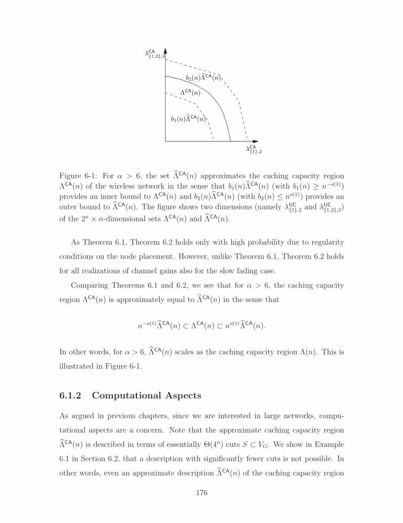
λCA

1,2,3

λCA

1,2

b1(n)ΛCA(n)

ΛCA(n)

b2(n)ΛCA(n)

Figure 6-1: For α > 6, the set ΛCA(n) approximates the caching capacity region

ΛCA(n) of the wireless network in the sense that b1(n)ΛCA(n) (with b1(n) ≥ n−o(1))

provides an inner bound to ΛCA(n) and b2(n)ΛCA(n) (with b2(n) ≤ no(1)) provides an

outer bound to ΛCA(n). The figure shows two dimensions (namely λUC

1,2 and λUC

1,2,3)

of the 2n × n-dimensional sets ΛCA(n) and ΛCA(n).

As Theorem 6.1, Theorem 6.2 holds only with high probability due to regularity

conditions on the node placement. However, unlike Theorem 6.1, Theorem 6.2 holds

for all realizations of channel gains also for the slow fading case.

Comparing Theorems 6.1 and 6.2, we see that for α > 6, the caching capacity

region ΛCA(n) is approximately equal to ΛCA(n) in the sense that

n−o(1)ΛCA(n) ⊂ ΛCA(n) ⊂ no(1)ΛCA(n).

In other words, for α > 6, ΛCA(n) scales as the caching capacity region Λ(n). This is

illustrated in Figure 6-1.

6.1.2 Computational Aspects

As argued in previous chapters, since we are interested in large networks, compu-

tational aspects are a concern. Note that the approximate caching capacity region

ΛCA(n) is described in terms of essentially Θ(4n) cuts S ⊂ VG. We show in Example

6.1 in Section 6.2, that a description with significantly fewer cuts is not possible. In

other words, even an approximate description ΛCA(n) of the caching capacity region

176

ΛCA(n) is computationally intractable for large values of n.

On the other hand, consider the simpler problem of testing membership of λCA ∈ΛCA(n). We now argue that this problem can be approximately solved in an efficient

manner. More precisely, we show that λCA ∈ ΛCA(n) can be checked approximately

in polynomial time in the description complexity of λCA. Combined with Theorem

6.1 and 6.2, this shows that for α > 6 approximate membership λCA ∈ ΛCA(n) can be

checked efficiently as well.

Formally, define for any caching traffic matrix λCA ∈ R2n×n+

ρλCA(n) , supρ ≥ 0 : ρλCA ∈ ΛCA(n).

Membership λCA ∈ ΛCA(n) can then be evaluated by checking if ρλCA(n) ≤ 1. Let

φλCA(n) to be the solution to the following linear program

max φ

s.t.∑

p∈PU,w

fp,U,w ≥ φλCAU,w ∀ U ⊂ V (n), w ∈ V (n),

∑

p∈P :e∈p

∑

U⊂V (n)

∑

w∈V (n)

fp,U,w ≤ ce ∀ e ∈ EG,

fp,U,w ≥ 0 ∀ U ⊂ V (n), w ∈ V (n), p ∈ PU,w,

(6.1)

where Pu,w is the path in G from node u to node w (since G is a tree, there is only

one such paths), and where

PU,w ,⋃

u∈U

Pu,w,

P ,⋃

U⊂V (n)

⋃

w∈V (n)

PU,w.

Note that the linear program (6.1), and hence also φλCA(n), can be evaluated in

polynomial time in the description length of λCA (i.e., in polynomial time in the

length of the “input” of the linear program) by setting the flow variables fp,U,w to

zero whenever λCAU,w = 0 and p ∈ PU,w. Moreover, using a primal-dual algorithm, (6.1)

177

can be solved efficiently in a distributed manner (see, for example, [41, Chapter 3.7]).

The following theorem shows that φλCA(n) is a good approximation to ρλCA(n).

Theorem 6.3. Under either fast or slow fading, for any α > 2, there exists b3 ≥n−o(1) such that for any n and caching traffic matrix λCA ∈ R

2n×n+

b3(n)ρλCA(n) ≤ φλCA(n) ≤ ρλCA(n).

As argued above, φλCA(n) can be computed in polynomial time in the description

length of λCA. Hence Theorem 6.3 shows that testing membership λCA ∈ ΛCA(n) can

be done approximately in polynomial time in the description length of λCA. Combined

with Theorems 6.1 and 6.2 this implies that, for α > 6, approximate achievability of a

traffic matrix λCA (i.e., testing membership λCA ∈ ΛCA(n)) can be checked efficiently

and in a distributed fashion.

6.2 Example Scenarios

Here we provide three examples illustrating various aspects of the caching capacity

region. Example 6.1 shows that the capacity region for caching is inherently more

complicated than the ones resulting from unicast or multicast traffic. Example 6.2

shows that the strategy of always selecting the nearest cache can be arbitrarily bad.

Example 6.3 analyzes the impact of complete caches on the performance of the wireless

network.

Example 6.1. Insufficiency of edge cuts

For unicast traffic and multicast traffic, we have seen in chapters 4 and 5 that it

is sufficient to consider edge cuts in G, i.e, cuts that result from removing a single

edge from G. By construction, G has at most 2n edges, and hence there are at most

2n such edge cuts. This contrasts with the situation for caching traffic, for which

Theorems 6.1 and 6.2 indicate that we have to consider general cuts, i.e., arbitrary

subsets S of VG. Indeed, the approximate capacity region ΛCA(n) is expressed in

terms of essentially Θ(4n) cuts. Comparing these two results, one might suspect that

178

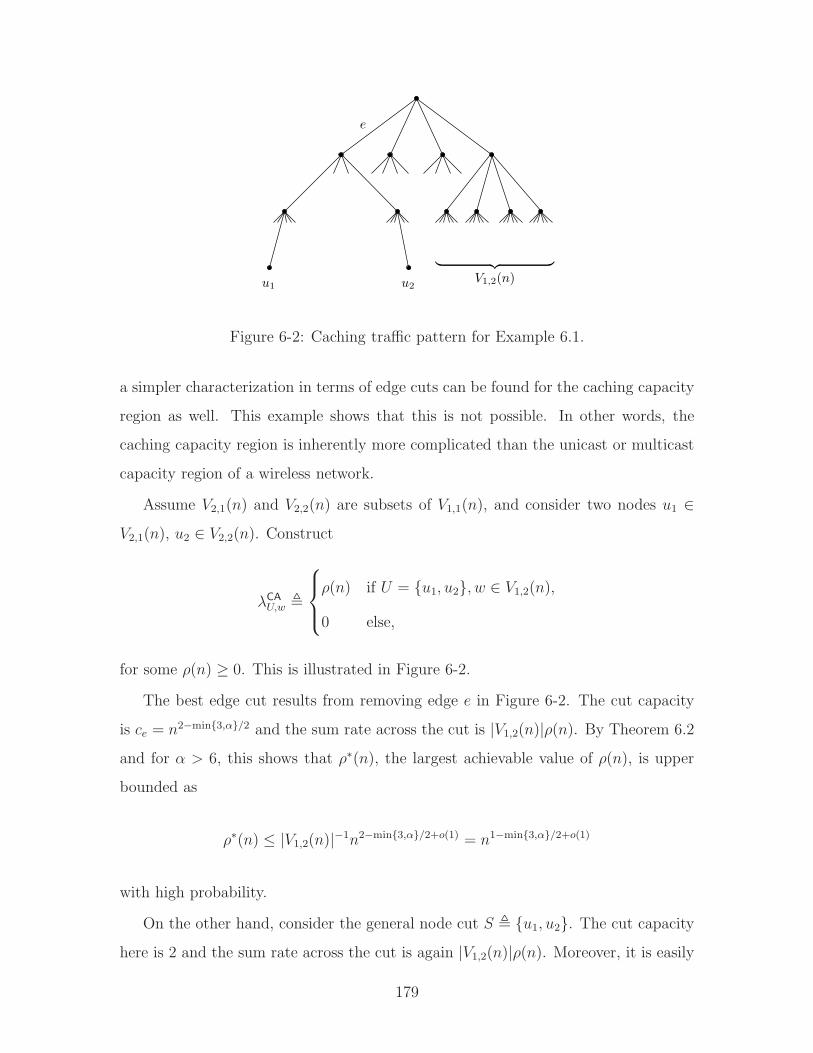
e

︸ ︷︷ ︸V1,2(n)u1 u2

Figure 6-2: Caching traffic pattern for Example 6.1.

a simpler characterization in terms of edge cuts can be found for the caching capacity

region as well. This example shows that this is not possible. In other words, the

caching capacity region is inherently more complicated than the unicast or multicast

capacity region of a wireless network.

Assume V2,1(n) and V2,2(n) are subsets of V1,1(n), and consider two nodes u1 ∈V2,1(n), u2 ∈ V2,2(n). Construct

λCA

U,w ,

ρ(n) if U = u1, u2, w ∈ V1,2(n),

0 else,

for some ρ(n) ≥ 0. This is illustrated in Figure 6-2.

The best edge cut results from removing edge e in Figure 6-2. The cut capacity

is ce = n2−min3,α/2 and the sum rate across the cut is |V1,2(n)|ρ(n). By Theorem 6.2

and for α > 6, this shows that ρ∗(n), the largest achievable value of ρ(n), is upper

bounded as

ρ∗(n) ≤ |V1,2(n)|−1n2−min3,α/2+o(1) = n1−min3,α/2+o(1)

with high probability.

On the other hand, consider the general node cut S , u1, u2. The cut capacity

here is 2 and the sum rate across the cut is again |V1,2(n)|ρ(n). Moreover, it is easily

179

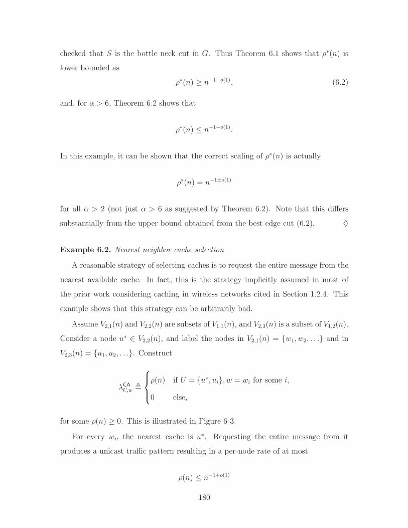
checked that S is the bottle neck cut in G. Thus Theorem 6.1 shows that ρ∗(n) is

lower bounded as

ρ∗(n) ≥ n−1−o(1), (6.2)

and, for α > 6, Theorem 6.2 shows that

ρ∗(n) ≤ n−1−o(1).

In this example, it can be shown that the correct scaling of ρ∗(n) is actually

ρ∗(n) = n−1±o(1)

for all α > 2 (not just α > 6 as suggested by Theorem 6.2). Note that this differs

substantially from the upper bound obtained from the best edge cut (6.2). ♦

Example 6.2. Nearest neighbor cache selection

A reasonable strategy of selecting caches is to request the entire message from the

nearest available cache. In fact, this is the strategy implicitly assumed in most of

the prior work considering caching in wireless networks cited in Section 1.2.4. This

example shows that this strategy can be arbitrarily bad.

Assume V2,1(n) and V2,2(n) are subsets of V1,1(n), and V2,3(n) is a subset of V1,2(n).

Consider a node u∗ ∈ V2,2(n), and label the nodes in V2,1(n) = w1, w2, . . . and in

V2,3(n) = u1, u2, . . .. Construct

λCA

U,w ,

ρ(n) if U = u∗, ui, w = wi for some i,

0 else,

for some ρ(n) ≥ 0. This is illustrated in Figure 6-3.

For every wi, the nearest cache is u∗. Requesting the entire message from it

produces a unicast traffic pattern resulting in a per-node rate of at most

ρ(n) ≤ n−1+o(1)

180

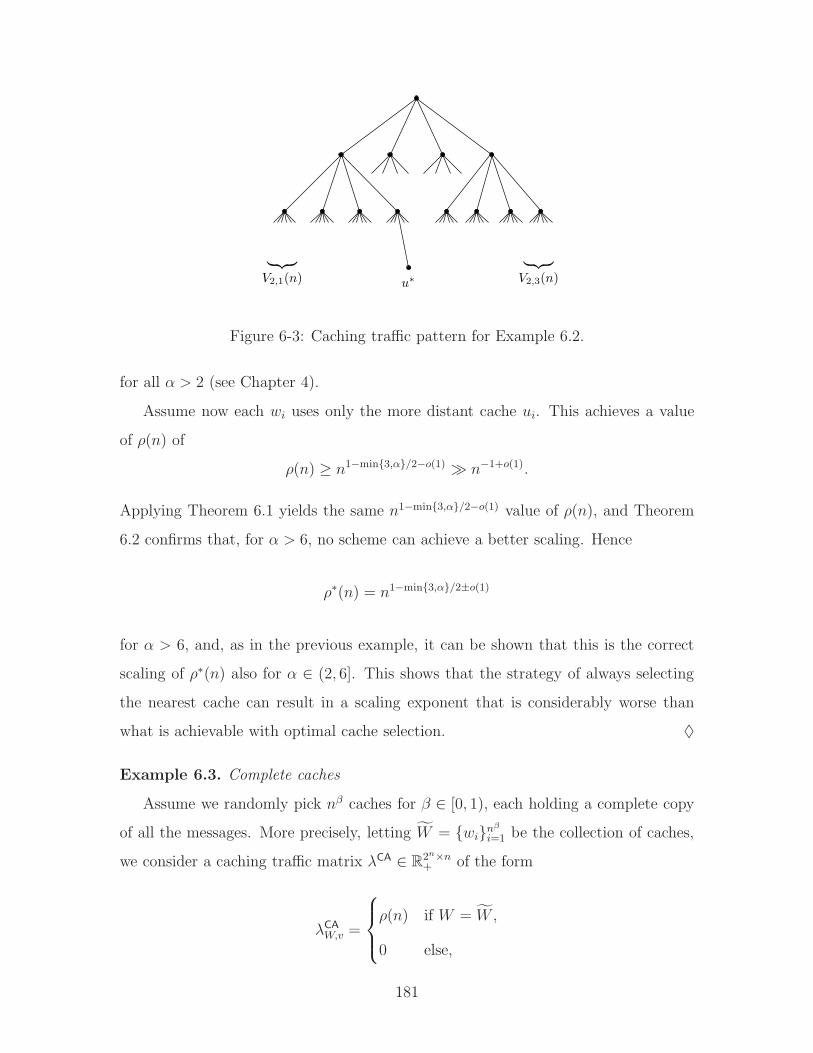
︸ ︷︷ ︸V2,1(n) u∗

︸ ︷︷ ︸V2,3(n)

Figure 6-3: Caching traffic pattern for Example 6.2.

for all α > 2 (see Chapter 4).

Assume now each wi uses only the more distant cache ui. This achieves a value

of ρ(n) of

ρ(n) ≥ n1−min3,α/2−o(1) ≫ n−1+o(1).

Applying Theorem 6.1 yields the same n1−min3,α/2−o(1) value of ρ(n), and Theorem

6.2 confirms that, for α > 6, no scheme can achieve a better scaling. Hence

ρ∗(n) = n1−min3,α/2±o(1)

for α > 6, and, as in the previous example, it can be shown that this is the correct

scaling of ρ∗(n) also for α ∈ (2, 6]. This shows that the strategy of always selecting

the nearest cache can result in a scaling exponent that is considerably worse than

what is achievable with optimal cache selection. ♦

Example 6.3. Complete caches

Assume we randomly pick nβ caches for β ∈ [0, 1), each holding a complete copy

of all the messages. More precisely, letting W = winβ

i=1 be the collection of caches,

we consider a caching traffic matrix λCA ∈ R2n×n+ of the form

λCA

W,v =

ρ(n) if W = W ,

0 else,

181

for some ρ(n) ≥ 0. In this setup, choosing the nearest cache strategy (as discussed in

Example 6.2) results in a per-node rate of

ρ(n) ≥ nβ−1−o(1)

with probability 1 − o(1) as n → ∞. The three-layer architecture proposed in The-

orem 6.1 achieves the same rate, and Theorem 6.2 shows that, for α > 6, for any

communication scheme

ρ(n) ≤ nβ−1+o(1).

Hence, for α > 6,

ρ∗(n) = nβ−1±o(1),

and it can be shown, as in the previous two examples, that this is the correct scaling

of ρ∗(n) also for α ∈ (2, 6].

This example illustrates that when in situations in which the traffic demand and

location of caches is regular enough, the strategy of selecting the nearest cache can

actually be close to optimal. ♦

6.3 Communication Scheme for Caching Traffic

Theorem 6.1 provides an inner bound to the caching capacity region of a wireless

network. Here we describe the communication scheme achieving this inner bound.

The matching outer bound shows that, for α > 6, this scheme is optimal in the scaling

sense.

The communication architecture uses the same three layer structure introduced in

4.3 for unicast traffic. Recall that, from high to low level of abstraction, these layers

are the routing layer, cooperation layer, and physical layer. Out of these three layers,

only the routing layer needs to be adapted for the transmission of caching traffic.

From the view of the routing layer, the wireless network consists of the noiseless

capacitated tree graph G (see Section 6.1.1 and Figure 4-3). To send a message at

182

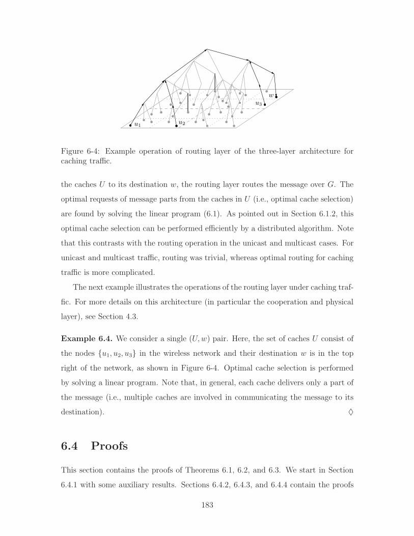
u1u2

u3

w

Figure 6-4: Example operation of routing layer of the three-layer architecture forcaching traffic.

the caches U to its destination w, the routing layer routes the message over G. The

optimal requests of message parts from the caches in U (i.e., optimal cache selection)

are found by solving the linear program (6.1). As pointed out in Section 6.1.2, this

optimal cache selection can be performed efficiently by a distributed algorithm. Note

that this contrasts with the routing operation in the unicast and multicast cases. For

unicast and multicast traffic, routing was trivial, whereas optimal routing for caching

traffic is more complicated.

The next example illustrates the operations of the routing layer under caching traf-

fic. For more details on this architecture (in particular the cooperation and physical

layer), see Section 4.3.

Example 6.4. We consider a single (U,w) pair. Here, the set of caches U consist of

the nodes u1, u2, u3 in the wireless network and their destination w is in the top

right of the network, as shown in Figure 6-4. Optimal cache selection is performed

by solving a linear program. Note that, in general, each cache delivers only a part of

the message (i.e., multiple caches are involved in communicating the message to its

destination). ♦

6.4 Proofs

This section contains the proofs of Theorems 6.1, 6.2, and 6.3. We start in Section

6.4.1 with some auxiliary results. Sections 6.4.2, 6.4.3, and 6.4.4 contain the proofs

183

of Theorems 6.3, 6.1, and 6.2, respectively.

6.4.1 Auxiliary Results

In this section, we define some quantities needed in several of the proofs.

We first introduce a “dual” description of the various regions. Recall that for any

caching traffic matrix λCA ∈ R2n×n+

ρλCA(n) , supρ ≥ 0 : ρλCA ∈ ΛCA(n)

.

Define similarly

ρλCA(n) , supρ ≥ 0 : ρλCA ∈ ΛCA(n)

.

Consider a caching traffic matrix λCA ∈ R2n×n+ for the wireless network and note that

λCA can equivalently be treated as a traffic matrix between the leaf nodes of the graph

G introduced in Section 6.1. Let ΛCAG (n) ⊂ R

2n×n+ be the collection of such caching

traffic matrices λCA ∈ R2n×n+ that can be transmitted over G using routing. Note that

φλCA(n) as defined through the linear program (6.1) is equal to

φλCA(n) = supφ ≥ 0 : φλCA ∈ ΛCA

G (n).

It can be shown that the regions ΛCA(n), ΛCA(n), and ΛCA

G (n) are convex, and hence

knowledge of ρλCA(n), ρλCA(n), and φλCA(n) for every λCA ∈ R2n×n+ is sufficient to

completely describe them.

Finally, recall the definition of the set V(n) of node placements V (n) that satisfy

certain regularity conditions as defined in Section 4.4.1.

6.4.2 Proof of Theorem 6.3

We first prove the upper bound, i.e.,

φλCA ≤ ρλCA. (6.3)

184

Note that if λCA ∈ ΛCA

G then there exists a strategy to route traffic at rates λCA over G.

This implies that the flow across each cut S ⊂ VG must be less than the capacity of

that cut. The flow across such a cut S contains at least all those requested messages

that have all their caches in S and their destination in Sc, i.e.,

∑

U⊂S∩V (n)

∑

w∈V (n)\SλCA

U,w.

On the other hand, the capacity of the cut S is equal to

∑

(u,v)∈EG:u∈S,v/∈S

cu,v.

Thus λCA ∈ ΛCA

G implies

∑

U⊂S∩V (n)

∑

w∈V (n)\SλCA

U,w ≤∑

(u,v)∈EG:u∈S,v/∈S

cu,v,

and hence λCA ∈ ΛCA. Therefore ΛCAG ⊂ ΛCA, from which (6.3) follows.

We now prove the lower bound, i.e., we show that there exists b3(n) ≥ n−o(1) such

that for any λCA

φλCA ≥ b3(n)ρλCA . (6.4)

Pick any λCA. Since for any b > 0,

φbλCA =1

bφλCA,

ρbλCA =1

bρλCA,

we may assume without loss of generality that

∑

(U,w)

λCA

U,w = 1. (6.5)

Recall that G is an undirected capacitated graph. Construct a directed capacitated

185

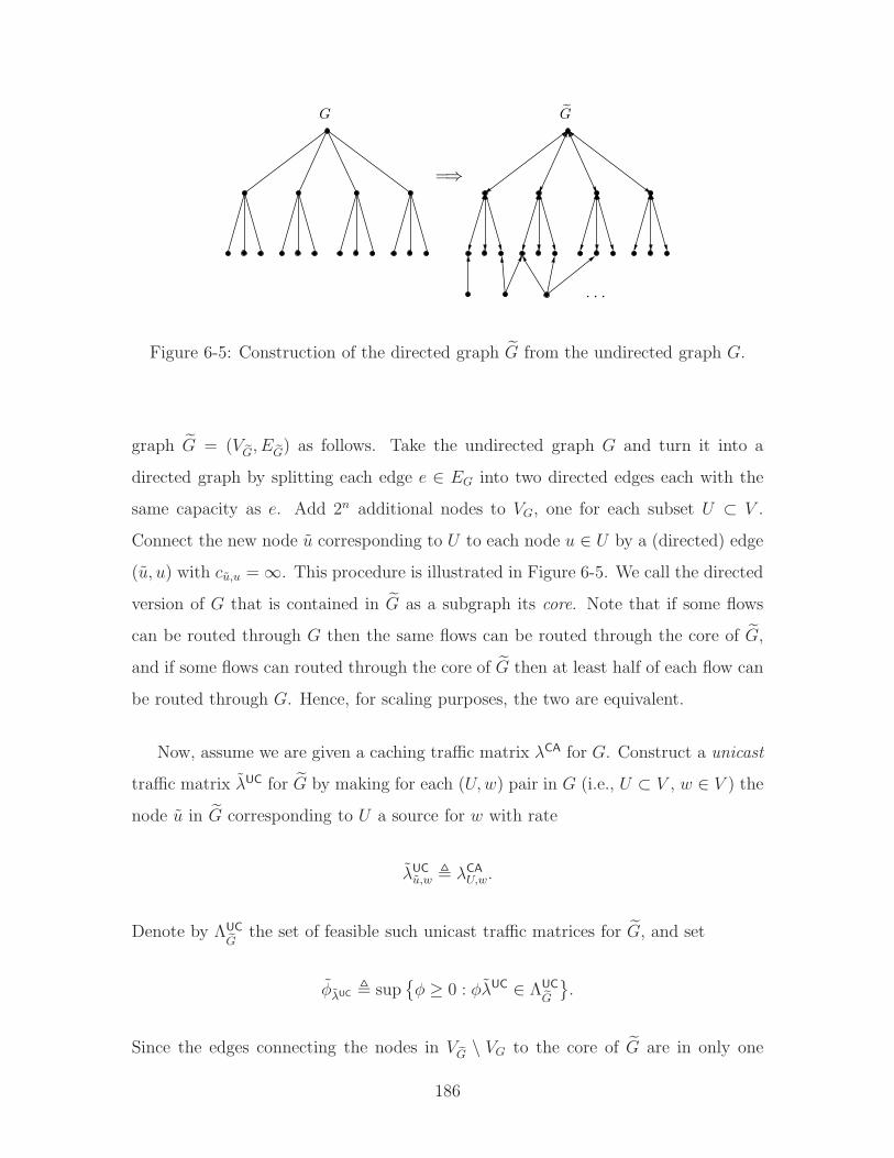
G G

. . .

=⇒

Figure 6-5: Construction of the directed graph G from the undirected graph G.

graph G = (V eG, E eG) as follows. Take the undirected graph G and turn it into a

directed graph by splitting each edge e ∈ EG into two directed edges each with the

same capacity as e. Add 2n additional nodes to VG, one for each subset U ⊂ V .

Connect the new node u corresponding to U to each node u ∈ U by a (directed) edge

(u, u) with cu,u = ∞. This procedure is illustrated in Figure 6-5. We call the directed

version of G that is contained in G as a subgraph its core. Note that if some flows

can be routed through G then the same flows can be routed through the core of G,

and if some flows can routed through the core of G then at least half of each flow can

be routed through G. Hence, for scaling purposes, the two are equivalent.

Now, assume we are given a caching traffic matrix λCA for G. Construct a unicast

traffic matrix λUC for G by making for each (U,w) pair in G (i.e., U ⊂ V , w ∈ V ) the

node u in G corresponding to U a source for w with rate

λUC

u,w , λCA

U,w.

Denote by ΛUC

eGthe set of feasible such unicast traffic matrices for G, and set

φλUC , supφ ≥ 0 : φλUC ∈ ΛUC

eG

.

Since the edges connecting the nodes in V eG \ VG to the core of G are in only one

186

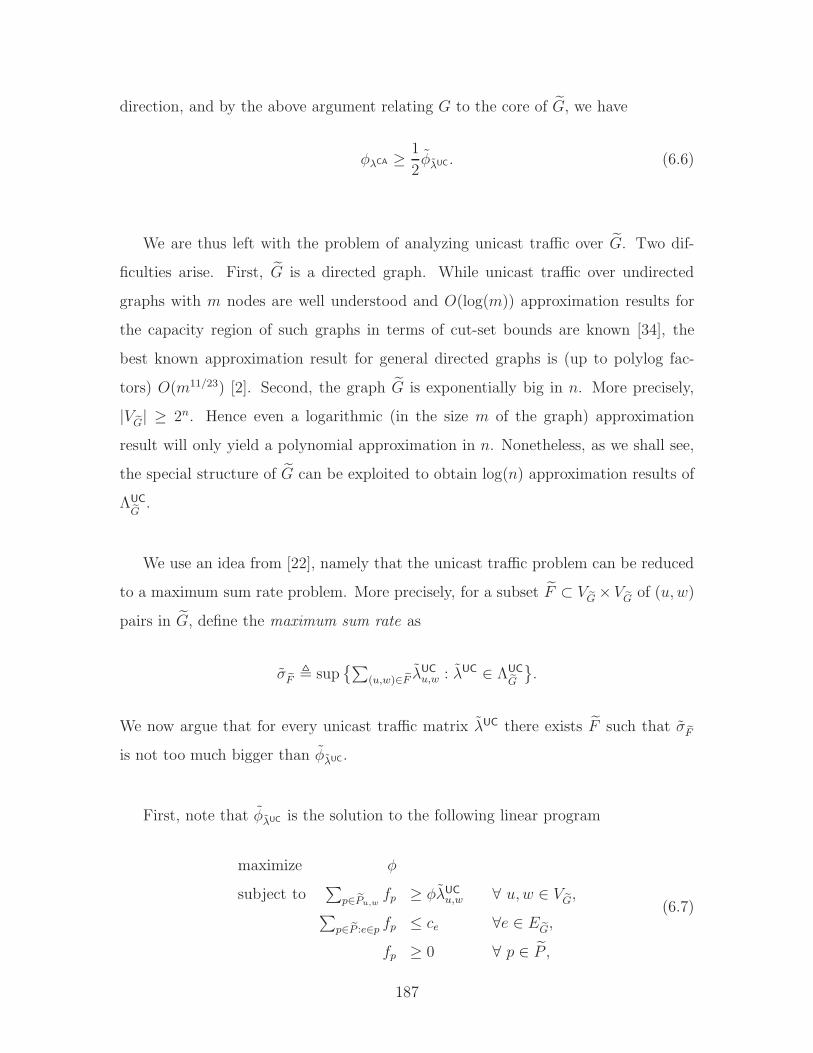
direction, and by the above argument relating G to the core of G, we have

φλCA ≥ 1

2φλUC . (6.6)

We are thus left with the problem of analyzing unicast traffic over G. Two dif-

ficulties arise. First, G is a directed graph. While unicast traffic over undirected

graphs with m nodes are well understood and O(log(m)) approximation results for

the capacity region of such graphs in terms of cut-set bounds are known [34], the

best known approximation result for general directed graphs is (up to polylog fac-

tors) O(m11/23) [2]. Second, the graph G is exponentially big in n. More precisely,

|V eG| ≥ 2n. Hence even a logarithmic (in the size m of the graph) approximation

result will only yield a polynomial approximation in n. Nonetheless, as we shall see,

the special structure of G can be exploited to obtain log(n) approximation results of

ΛUC

eG.

We use an idea from [22], namely that the unicast traffic problem can be reduced

to a maximum sum rate problem. More precisely, for a subset F ⊂ V eG × V eG of (u, w)

pairs in G, define the maximum sum rate as

σ eF , sup∑

(u,w)∈ eF λUC

u,w : λUC ∈ ΛUC

eG

.

We now argue that for every unicast traffic matrix λUC there exists F such that σ eF

is not too much bigger than φλUC .

First, note that φλUC is the solution to the following linear program

maximize φ

subject to∑

p∈ ePu,wfp ≥ φλUC

u,w ∀ u, w ∈ V eG,∑

p∈ eP :e∈p fp ≤ ce ∀e ∈ E eG,

fp ≥ 0 ∀ p ∈ P ,

(6.7)

187

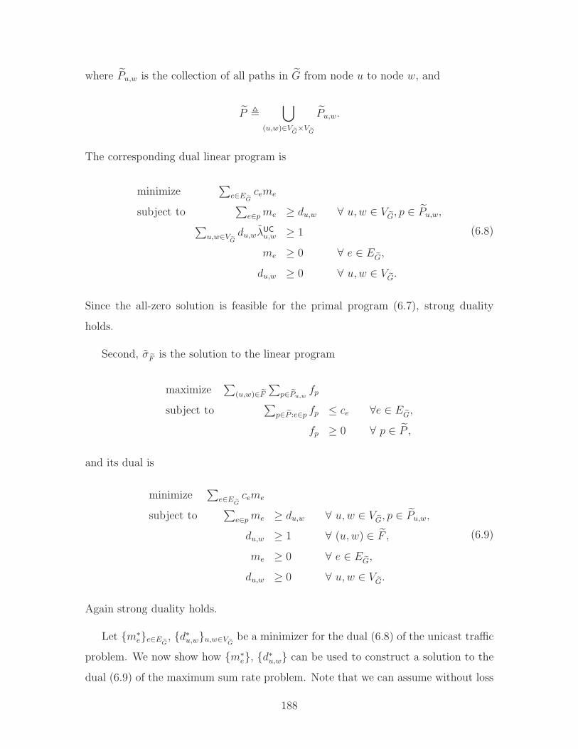
where Pu,w is the collection of all paths in G from node u to node w, and

P ,⋃

(u,w)∈V eG×V eG

Pu,w.

The corresponding dual linear program is

minimize∑

e∈E eGceme

subject to∑

e∈pme ≥ du,w ∀ u, w ∈ V eG, p ∈ Pu,w,∑

u,w∈V eGdu,wλ

UCu,w ≥ 1

me ≥ 0 ∀ e ∈ E eG,

du,w ≥ 0 ∀ u, w ∈ V eG.

(6.8)

Since the all-zero solution is feasible for the primal program (6.7), strong duality

holds.

Second, σ eF is the solution to the linear program

maximize∑

(u,w)∈ eF

∑p∈ ePu,w

fp

subject to∑

p∈ eP :e∈p fp ≤ ce ∀e ∈ E eG,

fp ≥ 0 ∀ p ∈ P ,

and its dual is

minimize∑

e∈E eGceme

subject to∑

e∈pme ≥ du,w ∀ u, w ∈ V eG, p ∈ Pu,w,

du,w ≥ 1 ∀ (u, w) ∈ F ,

me ≥ 0 ∀ e ∈ E eG,

du,w ≥ 0 ∀ u, w ∈ V eG.

(6.9)

Again strong duality holds.

Let m∗ee∈E eG

, d∗u,wu,w∈V eGbe a minimizer for the dual (6.8) of the unicast traffic

problem. We now show how m∗e, d∗u,w can be used to construct a solution to the

dual (6.9) of the maximum sum rate problem. Note that we can assume without loss

188

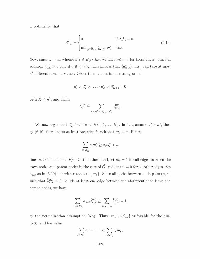
of optimality that

d∗u,w =

0 if λUCu,w = 0,

minp∈ ePu,w

∑e∈pm

∗e else.

(6.10)

Now, since ce = ∞ whenever e ∈ E eG \ EG, we have m∗e = 0 for those edges. Since in

addition λUCu,w > 0 only if u ∈ V eG \VG, this implies that d∗u,wu,w∈V eG

can take at most

n2 different nonzero values. Order these values in decreasing order

d∗1 > d∗2 > . . . > d∗K > d∗K+1 = 0

with K ≤ n2, and define

λUC

k ,∑

u,w∈V eG:d∗u,w=d∗k

λUC

u,w.

We now argue that d∗k ≤ n2 for all k ∈ 1, . . . , K. In fact, assume d∗1 > n2, then

by (6.10) there exists at least one edge e such that m∗e > n. Hence

∑

e∈E eG

cem∗e ≥ cem

∗e > n

since ce ≥ 1 for all e ∈ E eG. On the other hand, let me = 1 for all edges between the

leave nodes and parent nodes in the core of G, and let me = 0 for all other edges. Set

du,w as in (6.10) but with respect to me. Since all paths between node pairs (u, w)

such that λUCu,w > 0 include at least one edge between the aforementioned leave and

parent nodes, we have

∑

u,w∈V eG

du,wλUC

u,w ≥∑

u,w∈V eG

λUC

u,w = 1,

by the normalization assumption (6.5). Thus me, du,v is feasible for the dual

(6.8), and has value∑

e∈E eG

ceme = n <∑

e∈E eG

cem∗e,

189

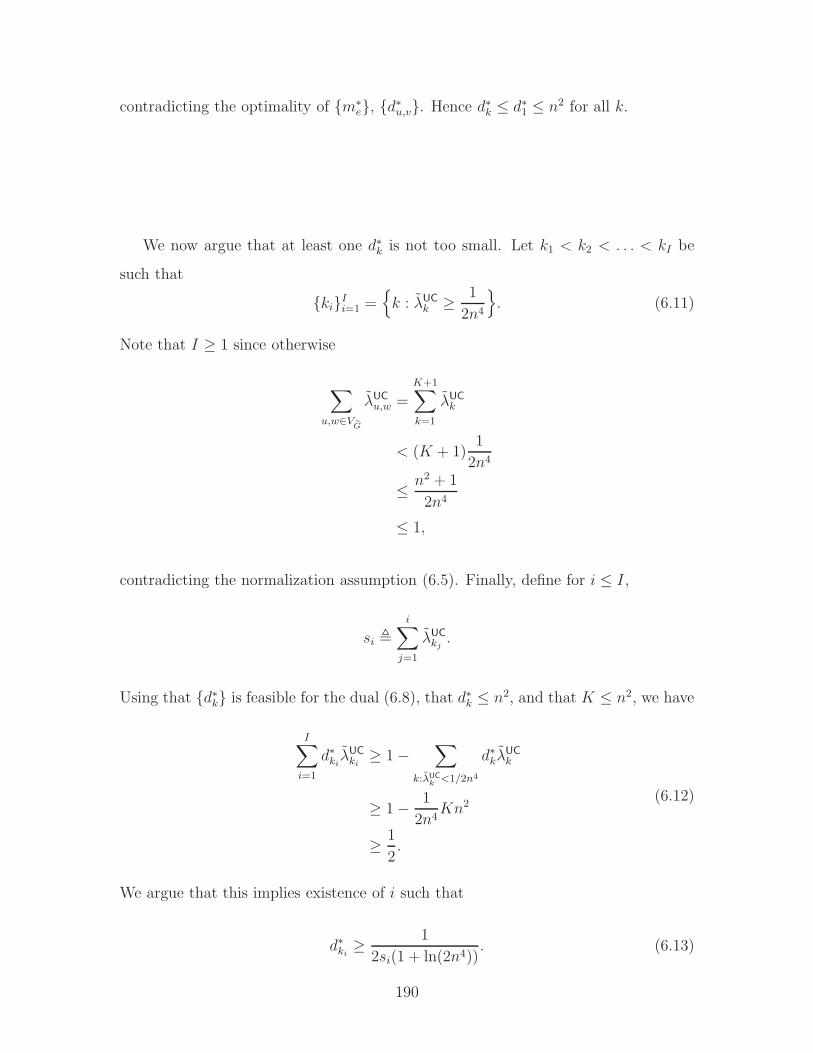
contradicting the optimality of m∗e, d∗u,v. Hence d∗k ≤ d∗1 ≤ n2 for all k.

We now argue that at least one d∗k is not too small. Let k1 < k2 < . . . < kI be

such that

kiIi=1 =

k : λUC

k ≥ 1

2n4

. (6.11)

Note that I ≥ 1 since otherwise

∑

u,w∈V eG

λUC

u,w =

K+1∑

k=1

λUC

k

< (K + 1)1

2n4

≤ n2 + 1

2n4

≤ 1,

contradicting the normalization assumption (6.5). Finally, define for i ≤ I,

si ,

i∑

j=1

λUC

kj.

Using that d∗k is feasible for the dual (6.8), that d∗k ≤ n2, and that K ≤ n2, we have

I∑

i=1

d∗kiλUC

ki≥ 1 −

∑

k:λUC

k <1/2n4

d∗kλUC

k

≥ 1 − 1

2n4Kn2

≥ 1

2.

(6.12)

We argue that this implies existence of i such that

d∗ki≥ 1

2si(1 + ln(2n4)). (6.13)

190

Indeed, assume (6.13) is false for all i. Then

I∑

i=1

d∗kiλUC

ki<

1

2(1 + ln(2n4))

I∑

i=1

λUC

ki

si

=1

2(1 + ln(2n4))

(1 +

I∑

i=2

si − si−1

si

)(6.14a)

≤ 1

2(1 + ln(2n4))

(1 +

I∑

i=2

(ln(si) − ln(si−1)

))(6.14b)

=1

2(1 + ln(2n4))

(1 + ln(sI/λ

UC

k1)))

≤ 1

2(1 + ln(2n4))

(1 + ln(2n4)

)(6.14c)

=1

2,

where we have used that I ≥ 1 in (6.14a), that 1 − x ≤ − ln(x) for every x ≥ 0 in

(6.14b), and that sI ≤ 1 by (6.5) and λUC

k1≥ 1

2n4 in (6.14c). This contradicts (6.12),

showing (6.13) must hold for some i. Consider this value of i in the following.

Now, consider the following set F of (u, w) pairs:

F ,(u, w) : d∗u,w ≥ d∗ki

.

Note that by (6.10) we have that if (u, w) ∈ F then u ∈ V eG \ VG and w is a “leaf”

node in VG. In other words, (u, w) pairs in F correspond to caches-destination pairs

(U,w) in G. Set for all u, w ∈ V eG and e ∈ E eG,

du,w ,d∗u,w

d∗ki

,

me ,m∗

e

d∗ki

.

Note that for (u, w) ∈ F ,

du,w =d∗u,w

d∗ki

≥ 1,

191

and that for all u, w ∈ V eG, p ∈ Pu,w,

∑

e∈p

me =1

d∗ki

∑

e∈p

m∗e

≥ 1

d∗ki

d∗u,w

= du,w,

by feasibility of d∗u,w and m∗e for the dual (6.8). Hence, for this F , the choice of

me and du,w is feasible for the dual (6.9).

By weak duality

σ eF ≤∑

e∈E eG

ceme

=1

d∗ki

∑

e∈E eG

cem∗e.

By (6.13),

d∗ki≥ 1

2si(1 + ln(2n4)),

and

si =i∑

j=1

λUC

kj

=i∑

j=1

∑

(u,w):d∗u,w=d∗kj

λUC

u,w

≤∑

(u,w):d∗u,w≥d∗ki

λUC

u,w

=∑

(u,w)∈ eF

λUC

u,w

, λUC

eF,

192

where in the third line we have used that d∗k1> d∗k2

> . . .. Therefore

σ eF ≤ 2λUC

eF(1 + ln(2n4))

∑

e∈E eG

cem∗e.

Since m∗e is optimal for the dual (6.8), and by strong duality, we also have

∑

e∈E eG

cem∗e = φλUC ,

and hence

φλUC ≥ 1

2(1 + ln(2n4))

σ eF

λUC

eF

. (6.15)

We are thus left with analyzing maximum sum rates σ eF . Now notice that since

the edges in E eG \ EG have infinite capacity, and since for (u, w) ∈ F we can assume

without loss of generality that u ∈ V eG \ VG, this analysis can be done by considering

only the core of G. More precisely, for a collection of node pairs F in G as above,

we construct a collection of node pairs F in G as follows. For each (u, w) ∈ F with

u connected by G with nodes U ⊂ VG ⊂ V eG, add (u, w) to F for each u ∈ U . Denote

by σF the maximum sum rate for F in G. Since G is the undirected version of the

core of G, we have

σ eF ≥ σF . (6.16)

For a collection of node pairs F in G, we call a set of edges M a multicut for F

if in the graph (VG, EG \M) each pair in F is disconnected. For a subset M ⊂ EG,

define

cM ,∑

e∈M

ce.

It is shown in [13, Theorem 8] that if G is an undirected tree, then for every F ∈VG × VG there exists a multicut M for F such that

σF ≥ 1

2cM . (6.17)

Combining (6.15), (6.16), and (6.17), we obtain that for every λUC there exists a

193

collection of node pairs F in G, and a multicut M for the corresponding F in G such

that

φλUC ≥ 1

4(1 + ln(2n4))

cM

λUC

eF

. (6.18)

We now show how the edge cut M ⊂ EG can be transformed into a node cut

S ⊂ VG. Denote by Si the connected components of (VG, EG \M). We have

∑

i

c(Sci ×Si)∩EG

≤ 2cM , (6.19)

since (Si×Sci )∩EG ⊂M for every i, and since every edge in M appears at most twice

in the sum on the left-hand side. With slight abuse of notation, define for S ⊂ VG

λCA

S,Sc ,∑

U⊂S∩V

∑

w∈V \SλCA

U,w.

M is a multicut for the F induced by F , and hence for every (u, w) ∈ F and the

corresponding pair (U,w), M separates w from all the nodes in U . Therefore, for

each such (U,w) pair, there exists a Si such that w ∈ Si, U ∩Si = ∅. This shows that

λUC

eF≤∑

i

λCA

Sci ,Si

. (6.20)

Equations (6.18), (6.19), and (6.20) imply that there exists j such that

φλUC ≥ 1

8(1 + ln(2n4))

∑i c(Sc

i ×Si)∩EG∑i λ

CASc

i ,Si

≥ 1

8(1 + ln(2n4))

c(Scj×Sj)∩EG

λCA

Scj ,Sj

≥ 1

8(1 + ln(2n4))minS⊂VG

c(S×Sc)∩EG

λCAS,Sc

=1

8(1 + ln(2n4))ρλCA .

(6.21)

194

Combined with (6.6), this shows that for

b3(n) ,1

16(1 + ln(2n4))≥ n−o(1)

we have

φλCA ≥ b3(n)ρλCA ,

proving the lower bound in Theorem 6.3.

6.4.3 Proof of Theorem 6.1

In this Section, we provide the proof of Theorem 6.1. Instead of proving the theorem

directly, it will be convenient to work with the dual description ρλCA(n) and ρλCA(n)

introduced in Section 6.4.1. The next theorem proves the dual version of Theorem

6.1.

Theorem 6.4. Under either fast or slow fading, for any α > 2, there exists b1 =

n−o(1) such that with probability 1− o(1) as n→ ∞ for any n and any caching traffic

matrix λCA ∈ R2n×n+

b1(n)ρλCA(n) ≤ ρλCA(n).

Proof. The same construction as in the proof of Theorem 4.10 shows that there exists

b(n) ≥ n−o(1) such that if a caching traffic matrix λCA can be routed over G, then

b(n)λCA can be communicated reliably over the wireless network. Formally, if V ∈ Vthen under fast fading

b(n)φλCA ≤ ρλCA , (6.22)

and the same results holds for slow fading for a collection of channel gains H (not

dependent on λCA) with

P(hu,vu,v∈V ∈ H) ≥ 1 − o(1)

as n→ ∞.

195

Combining (6.22), with Theorem 6.3 and Lemma 4.5, we obtain that with prob-

ability

P(hu,v ∈ H, V ∈ V) ≥ 1 − o(1)

as n→ ∞, we have for any caching traffic matrix λCA

ρλCA ≥ b(n)φλCA

≥ b(n)b3(n)ρλCA .

Setting

b1(n) , b(n)b3(n),

and recalling that b3(n) ≥ n−o(1) and b(n) ≥ n−o(1) both uniformly in λCA, concludes

the proof of Theorem 6.4.

6.4.4 Proof of Theorem 6.2

In this Section, we prove Theorem 6.2. As before, it will be convenient to work

with the dual description ρλCA(n) and ρλCA(n) introduced in Section 6.4.1. The next

theorem proves the dual version of Theorem 6.2

Theorem 6.5. Under either fast or slow fading, for any α > 2, there exists b2 ≤ no(1)

such that with probability 1−o(1) as n→ ∞ for any n and any caching traffic matrix

λCA ∈ R2n×n+

ρλCA(n) ≤ b2(n)ρλCA(n).

We start with some auxiliary lemmas. For a subsets S1, S2 ⊂ V (n), denote by

C(S1, S2) the MIMO capacity between the nodes in S1 and S2. Moreover, denote by

Sk2 the nodes in S2 that are at distance between k and k + 1 from S1, i.e.,

Sk2 , v ∈ S2 : min

u∈S1

ru,v ∈ [k, k + 1).

Lemma 6.6. Under either fast or slow fading, for every α > 6, there exists a constant

196

K1 such that for all V (n) ∈ V(n) and all S1, S2 ⊂ V (n), S2 ∩ S1 = ∅,

C(S1, S2) ≤ K1 log4(n)

log(n)∑

k=0

|Sk2 |.

Proof. Note that

S2 =

∞⋃

k=0

Sk2 ,

Let

HS1,S2 , [hu,v]u∈S1,v∈S2

be the matrix of channel gains between the nodes in S1 and S2. Under fast fading

C(S1, S2) , maxQ(H)≥0:

E(qu,u)≤P ∀u∈S1

E

(log det

(I + H

†S1,S2

Q(H)HS1,S2

)),

and under slow fading

C(S, Sc) , maxQ≥0:

qu,u≤P ∀u∈S1

log det(I + H

†S1,S2

QHS1,S2

).

Applying the generalized Hadamard inequality, we obtain that under either fast or

slow fading

C(S1, S2) ≤ C(S,∪log(n)k=0 Sk

2 ) + C(S,∪k>log(n)Sk2 ). (6.23)

For the first term in (6.23), using Hadamard’s inequality once more, yields

C(S1,∪log(n)k=0 Sk

2 ) ≤log(n)∑

k=0

∑

v∈Sk2

C(S1, v)

≤log(n)∑

k=0

∑

v∈Sk2

C(vc, v).

By Lemma 4.6,

C(vc, v) ≤ K log(n),

197

and thus

C(S1,∪log(n)k=0 Sk

2 ) ≤ K log(n)

log(n)∑

k=0

|Sk2 |. (6.24)

For the second term in (6.23), we have the following upper bound from (slightly

adapting) Theorem 2.1 in [21]:

C(S1,∪k>log(n)Sk2 ) ≤

∑

k>log(n)

∑

v∈Sk2

(∑

u∈S1

r−α/2u,v

)2

.

Consider v ∈ Sk2 . By the definition of Sk

2 , the (open) ball of radius k around v does

not contain any node in S1. Moreover, since V ∈ V, there are at most log(n) nodes

inside every square of sidelength one. Thus

∑

u∈S1

r−α/2u,v ≤ 4π(k + 2)2 log(n)k−α/2 + log(n)

∞∑

k=2k

10π(k + 2)k−α/2

≤ K log(n)k2−α/2,

for some constant K independent of S1 and k. Therefore,

C(S1,∪k>log(n)Sk2 ) ≤

∑

k>log(n)

|Sk2 |K2 log2(n)k4−α. (6.25)

Consider now some v ∈ Sk2 with k > log(n), and let u∗ be the closest point in S1

to v. Since v ∈ Sk2 , we must have

ru∗,v ∈ [k, k + 1).

Consider the (open) ball of radius ru∗,v around v and the ball of radius log(n) around

u∗. Since u∗ is the closest node to v in S1, all nodes in the ball around v are in S2.

Moreover, the intersection of the two balls has an area of at least π4

log2(n). Since

V ∈ V, this implies that this intersection must contain at least one point, say v, and

198

by construction

v ∈log(n)⋃

k=0

S k2 .

This shows that for every node v in Sk2 there exists a node v in ∪log(n)

k=0S k

2 such that

rv,v ∈ [k − log(n), k + 1).

Now, since V ∈ V, for every node v, there are at most

2π(k + 1)(log(n) + 6) log(n) ≤ K ′k log2(n)

nodes at distance [k− log(n), k+1) for some constant K ′. Hence the number of nodes

in Sk2 is at most

|Sk2 | ≤ K ′k log2(n)

log(n)∑

k=0

|S k2 |. (6.26)

Combining (6.26) with (6.25) yields

C(S1,∪k>log(n)Sk2 ) ≤

∑

k>log(n)

|Sk2 |K2 log2(n)k4−α

≤ K ′K2 log4(n)( log(n)∑

k=0

|S k2 |) ∑

k>log(n)

k5−α

= K ′′ log4(n)

log(n)∑

k=0

|S k2 |,

(6.27)

for some constant K ′′, and where we have used that α > 6. Finally, substituting

(6.24) and (6.27) into (6.23) shows that

C(S1, S2) ≤ (K +K ′′) log4(n)

log(n)∑

k=0

|Sk2 |,

which proves the lemma with

K1 , K +K ′′.

199

The next lemma shows that for large path-loss exponents (α > 6) every cut is

approximately achievable, i.e., for every cut there exists an achievable unicast traffic

matrix that has a sum rate across the cut that is not much smaller than the cut

capacity.

Lemma 6.7. Under fast fading, for every α > 6, there exists b4(n) ≤ no(1) such that

for V (n) ∈ V(n) and S ⊂ V (n) we can find a unicast traffic matrix λUC ∈ ΛUC(n)

satisfying

C(S, Sc) ≤ b4(n)∑

u∈S

∑

w/∈S

λUC

u,w. (6.28)

Moreover, there exists a collection of channel gains H(n) such that

P(hu,vu,v∈V (n) ∈ H(n)

)≥ 1 − o(1)

as n→ ∞, and such that for hu,vu,v ∈ H(n), (6.28) holds for slow fading as well.

Proof. By Lemma 6.6 for V ∈ V

C(S, Sc) ≤ K1 log4(n)|v ∈ Sc : rS,v < log(n) + 1|, (6.29)

where

rS,v , minu∈S

ru,v.

Construct a unicast traffic matrix λUC ∈ Rn×n+ as

λUC

u,w ,

ρ(n) if ru,w < log(n) + 1,

0 else,

for some function ρ(n). We now argue that for ρ(n) = Θ(log−2(n)) there exists

b(n) ≥ n−o(1) such that b(n)λUC ∈ ΛUC. This follows from Theorem 4.1, once we show

that for every ℓ ∈ 1, . . . , L(n) ∪ log(n) and i ∈ 1, . . . , 4ℓ we have

∑

u∈Vℓ,i

∑

w/∈Vℓ,i

λUC

u,w ≤ max1, 4−ℓn2−min3,α/2,

200

∑

u/∈Vℓ,i

∑

w∈Vℓ,i

λUC

u,w ≤ max1, 4−ℓn2−min3,α/2,

and

∑

u 6=w

λUC

u,w ≤ K log2(n)ρ(n) ∀w ∈ V,

∑

w 6=u

λUC

u,w ≤ K log2(n)ρ(n) ∀u ∈ V,

for some constant K. By the locality of the traffic matrix λUC, this is sufficient to

show that Theorem 4.1 applies for ρ(n) = 1K

log−2(n). Hence b(n)λUC ∈ ΛUC for fast

fading, and the same conclusion holds for slow fading for some H with

P(hu,vu,v∈V ∈ H

)≥ 1 − o(1)

as n→ ∞.

Combined with (6.29), this implies that

C(S, Sc) ≤ K log6(n)

b(n)

∑

u∈S

∑

w/∈S

λUC

u,w,

proving the lemma.

We are now ready for the proof of the outer bound on ΛCA(n).

Proof of Theorem 6.5. Consider a cut S ⊂ V in the wireless network. Assume we

allow the nodes on each side of the cut to cooperate without any restriction — this

can clearly only increase ρλCA . The total amount of traffic that needs to be transmitted

across the cut is then∑

W⊂S

∑

v/∈S

λCA

W,v.

The maximum achievable sum rate (with the aforementioned node cooperation) is

201

given by C(S, Sc) the MIMO capacity between the nodes in S and in Sc. Therefore

ρλCA ≤ minS⊂V

C(S, Sc)∑U⊂S

∑w/∈S λ

CAU,w

. (6.30)

We proceed by relating the cut S in the wireless network to a cut S in G. By

Lemma 6.7 for V ∈ V, there exists λUC ∈ ΛUC such that for fast fading

C(S, Sc) ≤ b4(n)∑

u∈S

∑

w/∈S

λUC

u,w, (6.31)

and (6.31) holds also for slow fading if hu,vu,v ∈ H (with H defined as in Lemma

6.7). By Theorem 4.2, for α > 5 and V ∈ V there exists K such that if λUC ∈ ΛUC

then K log−6(n)λUC ∈ ΛUC

G .

Now, consider any S ⊂ VG such that S ∩ V = S. Note that S is a cut in G

separating S from V \ S. Since K log−6(n)λUC ∈ ΛUCG , we thus have

∑

u∈S

∑

w/∈S

K log−6(n)λUC

u,w ≤∑

(u,v)∈EG:

u∈eS,v/∈eS

cu,v,

and by minimizing over the choice of S,

∑

u∈S

∑

w/∈S

K log−6(n)λUC

u,w ≤ mineS: eS∩V =S

∑

(u,v)∈EG:

u∈eS,v/∈eS

cu,v. (6.32)

Combining (6.31) and (6.32) shows that

C(S, Sc) ≤ b4(n)

Klog6(n) min

eS: eS∩V =S

∑

(u,v)∈EG:

u∈eS,v/∈eS

cu,v.

Together with (6.30), and using Lemmas 4.5 and 6.7, this yields that with prob-

ability

P(hu,vu,v ∈ H, V ∈ V) ≥ 1 − o(1)

202

as n→ ∞, we have for any caching traffic matrix λCA

ρλCA ≤ minS⊂V

C(S, Sc)∑U⊂S

∑w/∈S λ

CAU,w

≤ b2(n) minS⊂V

mineS∈VG: eS∩V =S

∑(u,v)∈EG:

u∈eS,v/∈eS

cu,v

∑U⊂eS∩V

∑w∈V \eS λ

CAU,w

= b2(n) mineS⊂VG

∑(u,v)∈EG:

u∈eS,v/∈eS

cu,v

∑U⊂eS∩V

∑w∈V \eS λ

CAU,w

= b2(n)ρλCA ,

with

b2(n) ,b4(n)

Klog6(n) ≤ no(1).

6.5 Discussion

Here we discuss extensions and implications of the results presented in this chapter.

In Section 6.5.1 we consider dense networks, and in Section 6.5.2 we discuss design

guidelines.

6.5.1 Dense Networks

The results presented so far in this chapter assumed extended node placement. Here

we discuss how these results can be modified for the dense case, where n nodes are

located on a square of area one.

As was the case for unicast and multicast traffic (see chapters 4 and 5), achievabil-

ity for dense networks (regardless of the value of path-loss exponent) can be derived

from the achievability result for extended networks by taking a limit as α→ 2. This

shows that for dense networks, for any α > 2, there exists b1(n) ≥ n−o(1) such that

with probability 1 − o(1)

b1(n)ΛCA(n) ⊂ ΛCA(n)

203

with

ΛCA(n) ,

λCA ∈ R

2n×n+ :

∑

U⊂S∩V (n)

∑

w∈V (n)\SλCA

U,w ≤∑

(u,v)∈EG:u∈S,v/∈S

cu,v ∀S ⊂ VG

,

and for an edge e at level ℓ in G,

ce ,

4−ℓn if 1 ≤ ℓ ≤ L(n),

1 if ℓ = L(n) + 1.

For the converse result, we need to replace Lemma 6.6 by the inequality

C(S, Sc) ≤ K log(n) min|S|, |Sc|

for some constant K, and we need to modify Lemma 6.7 accordingly. From this, we

obtain that for dense networks, for any α > 2, there exists b2(n) ≤ no(1) such that

with probability 1 − o(1)

ΛCA(n) ⊂ b2(n)ΛCA(n).

This is a stronger result than the corresponding upper bound for extended networks,

which was only shown to hold for α > 6.

In other words, for dense networks, for any value of path-loss exponent α > 2, we

have ΛCA(n) = n±o(1)ΛCA(n). Furthermore, in the dense setting, the expression for

ΛCA(n) can be simplified to

ΛCA(n) =

λCA ∈ R

2n×n+ :

∑

U⊂S

∑

w∈Sc

λCA

U,w ≤ min|S|, n− |S| ∀S ⊂ V (n)

.

Note that here we only consider subsets of V (n) (as opposed to VG(n)). Hence, for

the dense case ΛCA(n) provides a complete scaling characterization of the 2n × n-

dimensional caching capacity region ΛCA(n) in terms of Θ(2n) cuts (as opposed to

Θ(4n) cuts necessary for the description of ΛCA(n) for the extended case).

204

6.5.2 Design Guidelines

The results presented in this chapter suggest the following design guidelines for uti-

lizing caches in large wireless networks. First, as we have seen in Example 6.2, the

strategy of selecting only the closest cache can be quite bad in general. Instead, the

cache selection has to be done in a load-balanced fashion. In our proposed three-layer

architecture, cache selection is performed by solving a linear program. Moreover,

we argued that the solution to this linear program can be found efficiently by a

distributed algorithm. On the other hand, when the cache location and traffic are

already balanced enough (as is the case in Example 6.3), this load balancing can be

omitted, and closest cache selection can indeed be close to optimal.

Second, the results suggest that, at least in the large path-loss regime, the problem

of optimal cache selection can be solved at the routing layer. In other words, the

physical and cooperation layer are not affected by the introduction of caches.

6.6 Chapter Summary

We analyzed the influence of caching on the performance of wireless networks. Our

approach is information-theoretic, yielding a scaling characterization of the complete

caching capacity region in the high path-loss regime α > 6. Even though this region

is 2n × n dimensional (i.e., exponential in the number of nodes n in the wireless

network), we present an algorithm that checks approximate feasibility of a particular

caching traffic matrix efficiently (in polynomial time in the description length of the

caching traffic matrix). Achievability is proved using a three-layer communication

architecture achieving the entire caching capacity region in the scaling sense for α > 6.

The three layers deal with optimal selection of caches, choice of amount of necessary

cooperation, noise and interference, respectively. The matching (in the scaling sense)

converse proves that addressing these questions separately is without loss of order-

optimality in the regime of high path-loss exponent.

205

206

Chapter 7

Conclusions

This chapter contains concluding remarks. In Section 7.1 we summarize the results

presented in this thesis. Section 7.2 contains pointers for future work.

7.1 Thesis Summary

In this thesis, we have considered the impact of heterogeneities on achievable rates in

large wireless networks. Three types of such heterogeneities were discusses in detail:

location heterogeneity, traffic heterogeneity, and service heterogeneity.

We analyzed location heterogeneity be allowing the nodes in the wireless network

to be placed arbitrarily (with a minimum-separation constraint). This contrasts with

the standard homogeneity assumption, i.e., that nodes are placed independently and

uniformly at random. For the traffic model, we assumed random source-destination

pairing with uniform rate. We have seen that the impact of arbitrary node place-

ment depends strongly on the path-loss exponent α. For small path-loss exponents

α ∈ (2, 3], we showed that the node placement has no impact on achievable rates and

that global cooperation is necessary irrespective of the node placement. We proposed

a novel cooperative communication scheme (called hierarchical relaying), and showed

that it is order optimal for all node placements. For large path-loss exponents α > 3,

we have seen that the node placement critically impacts achievable rates as well as

optimal communication schemes. For very regular node placements, multi-hop com-

207

munication is order optimal, for very irregular node placements, hierarchical relaying

is optimal. We proposed a communication scheme “interpolating” between these two

schemes depending on the regularity of the node placement, and showed that this

scheme is order optimal under adversarial node placement with regularity constraint.

For traffic heterogeneity, we analyzed the n2-dimensional unicast capacity region

ΛUC(n). In other words, we allowed general unicast traffic. This contrasts with the

standard homogeneity assumption, i.e., that each node is source exactly once for a

destination chosen independently and uniformly at random from among all the other

nodes, and that all these n source-destination pairs communicate at equal rate. For

the node placement, we assumed that nodes are place independently and uniformly at

random. We presented inner an outer bounds on the unicast capacity region ΛUC(n).

These bounds coincide up to a factor n±o(1) along at least n2−n out of n2 dimensions

(corresponding to balanced traffic) for α ∈ (2, 5], and along all n2 dimensions for

α > 5. Hence, for α > 5, this provides a scaling characterization for the entire n2-

dimensional unicast capacity region ΛUC(n), and the same statement is true along at

least n2 −n dimensions for α ∈ (2, 5]. For the inner bound, we provided a three-layer

communication architecture. The three layers are the routing layer, the cooperation

layer, and the physical layer. In the routing layer, we perform load balancing —

dealing with the traffic heterogeneity. In the cooperation layer, we distribute and

concentrate traffic over the wireless network — choosing the appropriate amount of

cooperation. In the physical layer, we implement this distribution an concentration of

traffic — handling interference and noise. The approximate optimality of this scheme

(in the sense mentioned above) shows that these problems can be solved separately

without loss of order optimality.

For service heterogeneity, we analyzed the n× 2n-dimensional multicast capacity

region ΛMC(n) and the 2n × n-dimensional caching capacity region ΛCA(n). This

contrasts with the standard service homogeneity assumption, i.e., that all demands are

unicast. For the node placement, we again assumed that nodes a placed independently

and uniformly at random. We presented inner and outer bounds on ΛMC(n) and

ΛCA(n). For the multicast case, these bounds coincide up to a factor n±o(1) along

208

at least n2n − n out of n2n dimensions for α ∈ (2, 5], and along all n2n dimensions

for α > 5. Hence, for α > 5, this provides a scaling characterization of the entire

n×2n-dimensional multicast capacity region ΛMC(n), and the same statement is true

along at least n2n − n dimensions for α ∈ (2, 5]. For the caching case, these bounds

coincide up to a factor n±o(1) for α > 6, yielding a scaling characterization of the entire

2n × n-dimensional caching capacity region ΛCA(n) in the high path-loss regime. For

the inner bounds, we showed how the three-layer architecture proposed for general

unicast traffic can be modified to accommodate multicast and caching traffic. In both

cases, only the routing layer needed to be changed — the cooperation and physical

layer operate as in the unicast case.

7.2 Future Work

There are several directions for future work, of theoretical as well as practical interest.

The following questions are of theoretical interest, aiming at broadening our un-

derstanding of large heterogeneous wireless networks. First, note that the converse

for location heterogeneity in the α > 3 regime is only under adversarial node place-

ment with regularity constraint. One direction would be to find a converse for any

node placement. Second, for both unicast and multicast traffic, the scaling charac-

terization holds for all but n dimensions of the respective capacity regions in the

α ∈ (2, 5] regime. A second direction for future work is to complete the scaling char-

acterization for the remaining n dimensions in the low path-loss regime. Similarly, for

caching traffic, the results are only partial (namely only an inner bound is available)

for α ≤ 6. Completing the picture for α ≤ 6 would again be of interest. Third,

the results for traffic and service heterogeneity are derived assuming random node

placement. Obtaining scaling characterizations of the unicast or multicast capacity

regions under arbitrary node placement would be of interest. Ultimately, the goal is

to develop a complete scaling description of achievable rates in large heterogeneous

wireless networks.

The following questions and directions for future work are of practical interest.

209

First, most of the architectures presented in this thesis are centralized. To be im-

plementable in practice, decentralized architectures need to be developed. Second,

issues of delay have been completely ignored throughout this thesis. Especially in the

broadcast phase of the hierarchical relaying scheme, delays can be quite large. This

issue needs to be addressed before being implementable. Third, how to implement the

communication architectures proposed in this thesis within existing protocol stacks

needs to be addressed. For example, the distribution and concentration of traffic in

the cooperation layer of the three-layer architecture for traffic heterogeneity results in

growing header overhead. The design guidelines presented towards the end of the var-

ious chapters may be helpful in deciding which parts of the communication schemes

presented in this thesis are crucial for optimal operation of large wireless networks,

and which parts can be modified for simpler implementation.

210

Bibliography

[1] Shuchin Aeron and Venkatesh Saligrama. Wireless ad hoc networks: Strategiesand scaling laws for the fixed SNR regime. IEEE Transactions on InformationTheory, 53(6):2044–2059, June 2007.

[2] Amit Agarwal, Noga Alon, and Moses S. Charikar. Improved approximationfor directed cut problems. In Proceedings of the ACM Symposium on Theory ofComputing, pages 671–680, 2007.

[3] Ashish Agarwal and P. R. Kumar. Capacity bounds for ad hoc and hybrid wire-less networks. ACM SIGCOMM Computer Communications Review, 34(3):71–81, July 2004.

[4] Sahand Haji Ali Ahmad, Aleksandar Jovicic, and Pramod Viswanath. On outerbounds to the capacity region of wireless networks. IEEE Transactions on In-formation Theory, 52(6):2770–2776, June 2006.

[5] Joon Ahn and Bhaskar Krishnamachari. Fundamental scaling laws for energy-efficient storage and querying in wireless sensor networks. In Proceedings of theACM MobiHoc, pages 334–343, May 2006.

[6] Ivan Baev, Rajmohan Rajaraman, and Chaitanya Swamy. Approximation algo-rithms for data placement problems. 38(4):1411–1429, August 2008.

[7] Joao Barros and Sergio D. Servetto. Network information flow with correlatedsources. IEEE Transactions on Information Theory, 52(1):155–170, January2006.

[8] Thomas M. Cover, Abbas El Gamal, and Masoud Salehi. Multiple access chan-nels with arbitrarily correlated sources. IEEE Transactions on Information The-ory, 26(6):648– 657, November 1980.

[9] Thomas M. Cover and Joy A. Thomas. Elements of Information Theory. Wiley,1991.

[10] Massimo Franceschetti, Olivier Dousse, David N. C. Tse, and Patrick Thiran.Closing the gap in the capacity of wireless networks via percolation theory. IEEETransactions on Information Theory, 53(3):1009–1018, March 2007.

211

[11] Massimo Franceschetti, Marco D. Migliore, and Paolo Minero. The capacity ofwireless networks: Information-theoretic and physical limits. In Proceedings ofthe Allerton Conference on Communication, Control, and Computing, September2007.

[12] Massimo Franceschetti, Marco D. Migliore, and Paolo Minero. The degrees offreedom of wireless networks: Information theoretic and physical limits. In Pro-ceedings of the Allerton Conference on Communication, Control, and Computing,September 2008.

[13] Naveen Garg, Vijay V. Vazirani, and Mihalis Yannakakis. Primal-dual approxi-mation algorithms for integral flow and multicut in trees, with applications tomatching and set cover, pages 64–75. Lecture Notes in Computer Science.Springer, 1993.

[14] Piyush Gupta. Design and Performance Analysis of Wireless Networks. PhDthesis, University of Illinois at Urbana-Champaign, 2000.

[15] Piyush Gupta and P. R. Kumar. The capacity of wireless networks. IEEETransactions on Information Theory, 46(2):388–404, March 2000.

[16] Piyush Gupta and P. R. Kumar. Towards and information theory of large net-works: An achievable rate region. IEEE Transactions on Information Theory,49(8):1877–1894, August 2003.

[17] Te Sun Han. Slepian-Wolf-Cover theorem for network of channels. Informationand Control, 47(1):67–83, January 1980.

[18] Shunsuke Ihara. On the capacity of channels with additive non-Gaussian noise.Information and Control, 37(1):34–39, April 1978.

[19] Sang-Woon Jeon and Sae-Young Chung. Two-phase opportunistic broadcastingin large wireless networks. In Proceedings of the IEEE International Symposiumon Information Theory, pages 2771–2775, June 2007.

[20] Shudong Jin and Limin Wang. Content and service replication strategies inmulti-hop wireless mesh networks. pages 79–86, October 2005.

[21] Aleksandar Jovicic, Pramod Viswanath, and Sanjeev R. Kulkarni. Upper boundsto transport capacity of wireless networks. IEEE Transactions on InformationTheory, 50(11):2555–2565, November 2004.

[22] Nabil Kahale. On reducing the cut ratio to the multicut problem. UnpublishedManuscript, 1993.

[23] Alireza Keshavarz-Haddad, Vinay Ribeiro, and Rudolf Riedi. Broadcast capacityin multihop wireless networks. In Proceedings of the ACM MobiCom, pages 239–250, September 2006.

212

[24] Alireza Keshavarz-Haddad and Rudolf Riedi. On the broadcast capacity of mul-tihop wireless networks: Interplay of power, density and interference. In Pro-ceedings of the IEEE SECON, pages 324–323, June 2007.

[25] Alireza Keshavarz-Haddad and Rudolf Riedi. Multicast capacity of large homo-geneous multihop wireless networks. In Proceedings of the IEEE WiOpt, April2008.

[26] Ashish Khisti, Uri Erez, and Gregory W. Wornell. Fundamental limits and scal-ing behavior of cooperative multicasting in wireless networks. IEEE Transactionson Information Theory, 52(6):2762–2769, June 2006.

[27] Bong-Jun Ko and Dan Rubenstein. Distributed self-stabilizing placement ofreplicated resources in emerging networks. IEEE/ACM Transactions on Net-working, 13(3):476–487, June 2005.

[28] Gerhard Kramer, Michael Gastpar, and Piyush Gupta. Cooperative strategiesand capacity theorems for relay networks. IEEE Transactions on InformationTheory, 51(9):3037–3063, September 2005.

[29] Christof Krick, Harald Racke, and Matthias Westermann. Approximation algo-rithms for data management in networks. 36(5):497–519, October 2003.

[30] Sanjeev R. Kulkarni and Pramod Viswanath. A deterministic approach tothroughput scaling in wireless networks. IEEE Transactions on InformationTheory, 50(6):1041–1049, June 2004.

[31] Tom Leighton and Satish Rao. An approximate max-flow min-cut theorem foruniform multicommodity flow problems with applications to approximation al-gorithms. In Proceedings of the IEEE Symposium on Foundations of ComputerScience, pages 422–431, October 1988.

[32] Olivier Leveque and I. Emre Telatar. Information-theoretic upper bounds onthe capacity of large extended ad hoc wireless networks. IEEE Transactions onInformation Theory, 51(3):858–865, March 2005.

[33] Xiang-Yang Li, Shao-Jie Tang, and Ophir Frieder. Multicast capacity for largescale wireless ad hoc networks. In Proceedings of the ACM MobiCom, pages266–277, September 2007.

[34] Nathan Linial, Eran London, and Yuri Rabinovich. The geometry of graphs andsome of its algorithmic applications. Combinatorica, 15(2):215–245, June 1995.

[35] Ritesh Madan, Devavrat Shah, and Olivier Leveque. Product multicommod-ity flow in wireless networks. IEEE Transactions on Information Theory,54(4):1460–1476, April 2008.

213

[36] Pavan Nuggehalli, Vikram Srinivasan, and Carla-Fabiana Chiasserini. Energy-efficient caching strategies in ad hoc wireless networks. In Proceedings of theACM MobiHoc, pages 25–34, June 2003.

[37] Ayfer Ozgur, Olivier Leveque, and Emmanuel Preissmann. Scaling laws for one-and two-dimensional random wireless networks in the low-attenuation regime.IEEE Transactions on Information Theory, 53(10):3573–3585, October 2007.

[38] Ayfer Ozgur, Olivier Leveque, and David N. C. Tse. Hierarchical cooperationachieves optimal capacity scaling in ad hoc networks. IEEE Transactions onInformation Theory, 53(10):3549–3572, October 2007.

[39] Srinivas Shakkottai, Xin Liu, and R. Srikant. The multicast capacity of largemultihop wireless networks. In Proceedings of the ACM MobiCom, pages 247–255, September 2007.

[40] Birsen Sirkeci-Mergen and Michael Gastpar. On the broadcast capacity of wire-less networks. In Proceedings of the Information Theory and Applications Work-shop, January 2007.

[41] R. Srikant. The Mathematics of Internet Congestion Control. Birkhauser, 2003.

[42] Sundar Subramanian, Sanjay Shakkottai, and Piyush Gupta. On optimal ge-ographic routing in wireless networks with holes and non-uniform traffic. InProceedings of the IEEE INFOCOM, May 2007.

[43] Sundar Subramanian, Sanjay Shakkottai, and Piyush Gupta. Optimal geo-graphic routing for wireless networks with near-arbitrary holes and traffic. InProceedings of the IEEE INFOCOM, pages 2002–2010, April 2008.

[44] Bin Tang, Samir Das, and Himanshu Gupta. Cache placement in sensor networksunder update cost constraint. In Ad-Hoc, Mobile, and Wireless Networks, pages334–348. Springer, 2005.

[45] Bin Tang, Himanshu Gupta, and Samir R. Das. Benefit-based data caching in adhoc networks. IEEE Transactions on Mobile Computing, 7(3):289–304, March2008.

[46] Bulent Tavli. Broadcast capacity of wireless networks. IEEE CommunicationsLetters, 10(2):68–69, February 2006.

[47] L. G. Valiant and G. J. Brebner. Universal schemes for parallel communication.In Proceedings of the ACM Symposium on Theory of Computing, pages 263–277,1981.

[48] Liang-Liang Xie and P. R. Kumar. A network information theory for wirelesscommunication: Scaling laws and optimal operation. IEEE Transactions onInformation Theory, 50(5):748–767, May 2004.

214

[49] Liang-Liang Xie and P. R. Kumar. An achievable rate for the multiple-level relaychannel. IEEE Transactions on Information Theory, 51(4):1348–1358, April2005.

[50] Liang-Liang Xie and P. R. Kumar. On the path-loss attenuation regime forpositive cost and linear scaling of the transport capacity in wireless networks.IEEE Transactions on Information Theory, 52(6):2313–2328, June 2006.

[51] Feng Xue, Liang-Liang Xie, and P. R. Kumar. The transport capacity of wire-less networks over fading channels. IEEE Transactions on Information Theory,51(3):834–847, March 2005.

[52] Rong Zheng. Information dissemination in power-constrained wireless networks.In Proceedings of the IEEE INFOCOM, pages 1–10, April 2006.

215