Embed Size (px)
Citation preview
Page | 1 San Bernard Watershed Protection Plan December 2012
San Bernard River Watershed Protection Plan
Houston-Galveston Area Council
12/19/2012
Funding for the Development of this Watershed Protection Plan was provided by the Environmental Protection Agency through a federal American Recovery and Reinvestment Act (ARRA) grant to the Houston-Galveston Area Council, administered by the Texas Commission on Environmental Quality.

Page | 2 San Bernard Watershed Protection Plan December 2012
Table Of Contents
1 – Watershed Introduction ....................................................................................................................... 7
Watershed Protection Planning .................................................................................................................. 7
2 – Watershed Inventory and Characterization ......................................................................................... 9
Physical and Natural Features .................................................................................................................... 9
Watershed Boundaries ............................................................................................................................................................ 9
Topography .............................................................................................................................................................................. 9
Soils ........................................................................................................................................................................................ 11
Climate ................................................................................................................................................................................... 12
Wildlife and Habitat ............................................................................................................................................................... 13
Land cover and Population Characteristics .............................................................................................. 16
Land cover and Land Cover .................................................................................................................................................... 16
Existing Land Management Practices .................................................................................................................................... 18
Population Growth ................................................................................................................................................................ 18
Biology ................................................................................................................................................................................... 18
Geomorphology ..................................................................................................................................................................... 19
Additional Data Needed for Future Modeling ....................................................................................................................... 19
Sources of Information .......................................................................................................................................................... 19
3 – Public Participation ............................................................................................................................. 20
Public Participation ................................................................................................................................................................ 20
Public Participation Lead Agency Roles and Responsibilities ................................................................... 20
Stakeholder Facilitation ......................................................................................................................................................... 20
Project Partners ........................................................................................................................................ 21
project Partners ..................................................................................................................................................................... 21
Partners List ........................................................................................................................................................................... 21
WPP Stakeholder Group ........................................................................................................................... 21
Stakeholder Group Structure ................................................................................................................................................. 21
Agencies Involved as Stakeholders ........................................................................................................................................ 23
Citizens Involved as Stakeholders .......................................................................................................................................... 23
Goals Development ............................................................................................................................................................... 23
Selection of the Lead Organization for Implementation/Update of the WPP ....................................................................... 23
4 - Watershed Analysis ............................................................................................................................. 24

Page | 3 San Bernard Watershed Protection Plan December 2012
Hydrology ............................................................................................................................................................................... 24
Waterbody and Watershed Conditions .................................................................................................... 26
Water Quality Sampling ......................................................................................................................................................... 26
303(d) list ............................................................................................................................................................................... 28
Pollutant Sources ...................................................................................................................................... 29
Point Sources ......................................................................................................................................................................... 29
Nonpoint Sources .................................................................................................................................................................. 29
Identification of Causes and Sources ..................................................................................................................................... 35
Water Quality and Flow ......................................................................................................................................................... 38
Rainfall Information ............................................................................................................................................................... 40
Sources of Information .......................................................................................................................................................... 41
5 - Causes and Sources of Pollution (Element A) ...................................................................................... 42
Modeling Approach ............................................................................................................................................................... 42
SWAT Model .......................................................................................................................................................................... 43
Tidal Prism Modeling ............................................................................................................................................................. 43
Select Modeling ..................................................................................................................................................................... 43
POTENTIAL SOURCES OF BACTERIA ....................................................................................................................................... 45
Point Sources ......................................................................................................................................................................... 45
Non-Point Sources ................................................................................................................................................................. 46
SELECT MODELING CONCLUSIONS ........................................................................................................................................ 51
SWAT Modeling ..................................................................................................................................................................... 51
Above Tidal ............................................................................................................................................................................ 51
Below Tidal............................................................................................................................................................................. 52
6 – Estimated Load Reductions (Element B) ............................................................................................. 65
SWAT Model Performance .................................................................................................................................................... 65
Tidal Prism Model Performance ............................................................................................................................................ 66
Bacteria Source Analysis ........................................................................................................................................................ 68
BMP Scenario Evaluation ....................................................................................................................................................... 72
BMP Scenario 1 - Vegetative Filter Strips .............................................................................................................................. 72
BMP Scenario 2 - Grassed Water Ways ................................................................................................................................. 75
7 - Management Measures (Element C) ................................................................................................... 83
OSSFs ..................................................................................................................................................................................... 83
Wildlife ................................................................................................................................................................................... 83

Page | 4 San Bernard Watershed Protection Plan December 2012
Livestock ................................................................................................................................................................................ 84
Agriculture ............................................................................................................................................................................. 84
Wastewater Treatment Plants/Outfalls ................................................................................................................................. 84
Pets ........................................................................................................................................................................................ 85
Land Management ................................................................................................................................................................. 85
Model Ordinances.................................................................................................................................................................. 86
8 – Technical and Financial Needs (Element D) ........................................................................................ 87
OSSFs ..................................................................................................................................................................................... 87
Wildlife ................................................................................................................................................................................... 87
Livestock ................................................................................................................................................................................ 87
Agriculture ............................................................................................................................................................................. 87
Wastewater Treatment Plants/Outfalls ................................................................................................................................. 88
Urban Runoff ......................................................................................................................................................................... 88
Pets ........................................................................................................................................................................................ 88
Land Management ................................................................................................................................................................. 88
New Ordinances and Plans .................................................................................................................................................... 89
Sources of Funding................................................................................................................................................................. 89
9 – Outreach and Education (Element E) .................................................................................................. 90
Outreach and Education ........................................................................................................................................................ 90
Public Outreach and Education ................................................................................................................ 90
Advertising ............................................................................................................................................................................. 90
Media Relations ..................................................................................................................................................................... 90
Education ............................................................................................................................................................................... 92
10 – Project Implementation and Interim Milestones for Progress (Elements F & G) ............................ 96
OSSFs ..................................................................................................................................................................................... 96
Wastewater Treatment Plants/Outfalls ................................................................................................................................. 99
Wildlife/Pets ........................................................................................................................................................................ 101
Livestock and Agriculture ..................................................................................................................................................... 102
Land Management ............................................................................................................................................................... 104
11 – Water Quality Monitoring and Measures of Success (elements H & I) .......................................... 106
Project Goals ........................................................................................................................................................................ 106
Measures of Success ............................................................................................................................................................ 106
Project Description .............................................................................................................................................................. 106

Page | 5 San Bernard Watershed Protection Plan December 2012
San Bernard Watershed Protection Plan Appendices ............................................................................ 114
SELECT Model Assumptions ................................................................................................................................................. 114
Forecast of Sources by 2006 Land Cover Type .................................................................................................................... 115
Watershed Model – SWAT ................................................................................................................................................... 117
Receiving Water Model ....................................................................................................................................................... 133
Nine Element Table ……………………………………………………………………………………………………………………………………………………….143

Page | 6 San Bernard Watershed Protection Plan December 2012
LIST OF ACRONYMS
AWRL Ambient Water Reporting Limit
BMP Best Management Practice
CRP Clean Rivers Program
CWA Clean Water Act
DO Dissolved Oxygen
EPA Environmental Protection Agency
FEMA Federal Emergency Management Agency
GIS Geographic Information System
GPS Global Positioning System
H-GAC Houston-Galveston Area Council
LA Load Allocation
NCDC National Climatic Data Center
NELAC National Environmental Laboratory Accreditation Conference
NOAA National Oceanic Atmospheric Administration
NOS National Ocean Survey
NPDES National Pollutant Discharge Elimination System
NPS Nonpoint Source
PS Point Source
SLOC Station Location
SOP Standard Operating Procedure
SWQM Surface Water Quality Monitoring
SWQMIS Surface Water Quality Monitoring Information System
TCEQ Texas Commission on Environmental Quality
TSWQS Texas Surface Water Quality Standards
WQI Water Quality Inventory

Page | 7 San Bernard Watershed Protection Plan December 2012
1 – WATERSHED INTRODUCTION
WATERSHED PROTECTION PLANNING The San Bernard Watershed Protection Plan process was started in September 2009. Portions of the San
Bernard River do not meet contact recreation standards due to elevated bacteria levels, and they have been
placed on the TCEQ list of impaired waters (303d). There are also sections of the San Bernard that have
excessive nutrients and low dissolved oxygen, which may negatively affect fish and other aquatic life. Over the
course of the project, the Houston-Galveston Area Council has worked with community organizations, citizens,
government agencies, and local industries. The overall goal of the WPP is to identify the causes and sources of
water quality impairments and to bring water quality standards into compliance with state criteria. This WPP
was conducted to bring the water quality up to acceptable standards on a voluntary basis before it declined to
the point where a TMDL would be required.
The San Bernard Watershed Protection Plan is a study of the entire watershed to identify pollutant sources and
causes, and to form an action plan to control the pollutants entering the waterways. This plan integrates a
number of studies to determine what may be causing changes in water quality. Ambient water quality
monitoring has been going on in the watershed in some locations for as many as forty years, and a few studies
have been done on the river to assess habitats and flooding. This Watershed Protection Plan is a stakeholder
driven process, which provides an opportunity for the local leadership to guide the process so that the outcome
fits for their specific watershed and plans for potential future growth without further impairing the water
quality. The population of the watershed is expected to more than double in the next thirty years, which could
potentially have major impacts on water quality. Once completed, this plan will be approved by the Texas
Commission on Environmental Quality (TCEQ) and the Environmental Protection Agency (EPA).
Watershed Protection Plans address the causes and sources of pollution in watersheds. There are two types of
pollution in the watershed: point source and non-point source. Point source pollution comes from a known
source such as an outfall from a wastewater treatment facility. Point sources are generally regulated by state
and federal laws and require a permit. Nonpoint source pollution is the collection of all of the other runoff that
flows into the waterways including agricultural uses, residential uses, commercial uses, and natural areas. When
rainwater flows across the land in a watershed it takes with it all contaminants that are left behind by everyday
uses. Since nonpoint source pollution is a combination of many types of pollutants, it is hard to determine
where it is coming from and it is difficult to regulate. The vast majority of the San Bernard Watershed is devoted
to agricultural uses and has scattered areas of residential development, with a few more dense residential
developments in the tidal portion of the watershed. Many areas of the tidal portion of the river are used for
recreation by local residents. Some of the upper portions of the watershed have very low flow due to
overgrowth of vegetation along the waterways or siltation due to lack of vegetation.
The San Bernard Watershed Protection Plan gives the local decision makers the tools necessary to improve
water quality in the region, prepare for growth, incorporate Best Management Practices (BMPs), and coordinate
the framework for implementing and integrating protection and restoration strategies. This plan also identifies
management techniques, sources of funding, and technical assistance for the problems identified in the
watershed based on modeling efforts and expected population growth. The Watershed Protection Plan (WPP)

Page | 8 San Bernard Watershed Protection Plan December 2012
will follow the Nine Key Elements of watershed based plans as required by the Environmental Protection Agency
(EPA). Stakeholders have been very active in the watershed and were instrumental in the development of this
Watershed Protection Plan and will continue to be the major force that drives the implementation of this plan.
FIGURE 1.1 – SAN BERNARD WATERSHED BETWEEN AUSTIN AND COLORADO COUNTIES

Page | 9 San Bernard Watershed Protection Plan December 2012
2 – WATERSHED INVENTORY AND CHARACTERIZATION
PHYSICAL AND NATURAL FEATURES
WATERSHED BOUNDARIES
The San Bernard River Watershed is over 125 miles long and covers approximately 900 square miles. The headwaters of the San Bernard River originate in New Ulm in Austin County. The river flows through Austin, Colorado, Wharton, Fort Bend, and Brazoria Counties. The river ultimately drains to the Gulf of Mexico, just past the Intercoastal Waterway. The San Bernard River watershed is bounded on the north and east by the Brazos River basin and on the south and west by the Colorado River basin and Caney Creek. The San Bernard River comprises two stream segments defined by TCEQ. Stream segment 1302 is the San Bernard River above-tidal, which flows from the town of New Ulm in Austin County to a point 2.0 mi upstream of State Highway 35 in Brazoria County. Stream segment 1301 is San Bernard River tidal, which flows from 2.0 mi upstream of State Highway 35 in Brazoria County to the Gulf of Mexico in Brazoria County.
FIGURE 2.1 - LOCATION OF SAN BERNARD WATERSHED
TOPOGRAPHY
The terrain throughout the watershed is characterized by level to undulating plains rising to the north with a timber belt of hardwoods along the river. Closer to the mouth of the river the terrain is Bay Prairie where

Page | 10 San Bernard Watershed Protection Plan December 2012
prairie grasses, bunch grasses, mesquite, and oak predominate. Elevations in the watershed vary between 0” to 400”. The San Bernard Watershed is ideally suited for farming and ranching as the land is fairly flat. The lower portion of the watershed near the Gulf Coast is characterized by Gulf Coast Prairies and Marshes Ecoregion. Elevation is generally 5 feet or less above mean sea level with a few areas 10 feet or more above sea level. The Texas Gulf Coast has low-lying coastal landforms that include barrier islands, peninsulas, offshore sand bars, bays, mudflats, dunes, and shoals. These landforms are subject to the activities of waves, winds, storms, tides, climate, rising sea levels, and human activities.
FIGURE 2.2 – WATERSHED ELEVATION

Page | 11 San Bernard Watershed Protection Plan December 2012
FIGURE 2.2 - SAN BERNARD WATERSHED TOPOGRAPHY
SOILS
Soils include sand and gravels, sandy clay and silt with local sand, mud and other fluvial deposits. In the lower portion of the watershed near the Gulf, soils are primarily clays ranging from saline to non-saline. The land is nearly level and poorly drained. The lower portion of Brazoria County is in the Gulf Coast Marsh Resource Area and is predominantly salty soils. Most of the soils in the county are clayey and loamy, dark in color and have very little slope. 82% of the county is deep, non-saline soils. The major soils in the county are: Aris, Asa, Bernard, Brazoria, Edna, Lake Charles, Norwood, and Pledger. The Asa and Norwood soils are loamy and well drained, but the remainder of the soils is more poorly drained and has very slowly permeable subsoil. These soils are good for agricultural uses – row crops and pastures, and perform best with a surface drainage system. In Wharton County, soils range in slope from 1% to 8%, most are somewhat poorly drained, have moderate available water capacity, and have very low to moderately low permeability. Soil types include: Telferner fine sandy loam, Gladewater soils, Edna fine sandy loam, Hockley fine sandy loam, Fulshear-Kenney complex, and Bernard-Edna complex.

Page | 12 San Bernard Watershed Protection Plan December 2012
FIGURE 2.4 – SAN BERNARD WATERSHED SOILS
CLIMATE
Average annual rainfall in the area is between 40” to 54” with increasing levels towards the coast. The portion of the watershed along the coast is characterized by rainfall throughout the year with 60% falling between April and September. Average annual rainfall along the coast is 52 inches. There are a few rain gauges located throughout the watershed at the Atwater Prairie Chicken refuge, the City of Wharton, and at East Bernard.
Weather data for the simulation was collected from five weather stations in and around the San Bernard
Watershed: Brenham, Bellville, Wharton, Wharton Airport, and Freeport. Specific information on each type of
weather data is provided in more detail subsequently.
Although precipitation data were collected from the five stations noted previously, three stations (Bellville, Wharton, and Freeport) are located closest to the watershed. Therefore, data from these three stations were used preferentially to generate most of the precipitation input for SWAT modeling. A map of these three stations can be found on page 114 of the appendices. If there were gaps in the data during the simulation period the other two stations were used to complete these gaps. During the review of the weather data, one key discrepancy was noted for the precipitation data collected for Wharton County. One value noted on July 27, 2008 was noted to have a total of 13.98 inches of rainfall occurring but it could not be verified with other data sources such as NOAA, nearby weather stations. As such, it was removed from the rainfall dataset.
Page | 13 San Bernard Watershed Protection Plan December 2012
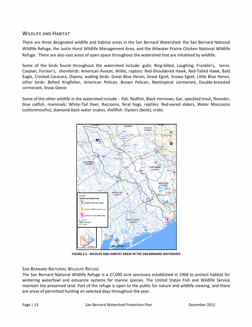
WILDLIFE AND HABITAT
There are three designated wildlife and habitat areas in the San Bernard Watershed: the San Bernard National
Wildlife Refuge, the Justin Hurst Wildlife Management Area, and the Attwater Prairie Chicken National Wildlife
Refuge. There are also vast areas of open space throughout the watershed that are inhabited by wildlife.
Some of the birds found throughout the watershed include- gulls: Ring-billed, Laughing, Franklin’s, terns: Caspian, Forster’s, shorebirds: American Avocet, Willet, raptors: Red-Shouldered Hawk, Red-Tailed Hawk, Bald Eagle, Crested Caracara, Osprey, wading birds: Great Blue Heron, Great Egret, Snowy Egret, Little Blue Heron, other birds: Belted Kingfisher, American Pelican, Brown Pelican, Neotropical cormorant, Double-breasted cormorant, Snow Geese Some of the other wildlife in the watershed include - fish: Redfish, Black minnows, Gar, speckled trout, flounder, blue catfish, mammals: White-Tail Deer, Raccoons, feral hogs, reptiles: Red-eared sliders, Water Moccasins (cottonmouths), diamond-back water snakes, shellfish: Oysters (beds), crabs.
FIGURE 2.5 - WILDLIFE AND HABITAT AREAS IN THE SAN BERNARD WATERSHED
SAN BERNARD NATIONAL WILDLIFE REFUGE
The San Bernard National Wildlife Refuge is a 27,000 acre sanctuary established in 1968 to protect habitat for wintering waterfowl and estuarine systems for marine species. The United States Fish and Wildlife Service maintain the preserved land. Part of the refuge is open to the public for nature and wildlife viewing, and there are areas of permitted hunting on selected days throughout the year.

Page | 14 San Bernard Watershed Protection Plan December 2012
A portion of this refuge is in the southernmost part of the San Bernard watershed, and is an important coastal marsh wilderness and shelter for millions of migrating and nesting birds, including over 230 different species annually. Some of these include snow geese, warblers, herons, egrets, terns, and gulls, as well as neotropical bird species. The birds can be found in the marshy bottomlands, on several remote islands, or within the bottomland hardwood forests found throughout the refuge. Visitors may also see bobcats or alligators while touring the wildlife sanctuary. The refuge also supports estuaries that flourish with shell and fin fish and reefs of colonial oysters, supplying a feeding ground for adult fish and crabs.
JUSTIN HURST WILDLIFE MANAGEMENT AREA
Justin Hurst Wildlife Management area (formerly The Peach Point Wildlife Management Area) is another coastal preserve found in the southernmost portion of the San Bernard River watershed. The land, acquired between 1985 and 1988, is dedicated to sound biological conservation of all wildlife resources for the public’s benefit. The WMA, managed by the Texas Parks and Wildlife Department, contains over 10,000 acres of coastal prairie and marshes and is part of the Central Coast Wetlands Ecosystem Project (CCWEP).
The CCWEP aims to create and maintain habitat for indigenous and migratory species, particularly waterfowl. Research activities are prevalent throughout the WMA, with resulting information concerning the understanding of coastal ecosystems distributed to scientists, land managers, resource agencies, and other interested parties. Currently, researchers are studying small mammals, snakes, and vegetation within the WMA. In addition, researchers assist in bird banding, which provides data for the Monitoring Avian Productivity and Survivorship Program. The San Bernard National Wildlife Refuge and the Justin Hurst Wildlife Management Area serve important functions in the conservation of native vegetation and migrating wildlife and in the understanding of coastal ecosystems. These sanctuaries not only provide important information to scientists and the public, but they also provide recreational opportunities for locals and tourists as well as economic benefits to the region.
ATTWATER’S PRAIRIE CHICKEN NATIONAL WILDLIFE REFUGE
The Attwater’s Prairie Chicken National Wildlife Refuge is located near Eagle Lake. Today it includes about 10,000 acres of protected habitat. In 1983, the US Fish and Wildlife Service formed the Attwater’s Prairie Chicken Recovery Team to carry out science-based efforts to help save the birds. As of 2009, 90 birds inhabit three reserve sites, but recovery efforts are still underway.
IN THE CENTRAL PORTION OF THE WATERSHED
Baldcypress wetlands, and green ash and water hickory trees dominate the landscape in the southern half of the San Bernard area while green ash and water oak are the predominate woody species in the northern half of the San Bernard study area and the Middle Bernard Creek area. Where present, yaupon holly and Chinese privet dominate the understory layer with a dense herbaceous layer throughout the area. Vegetation within the areas can be classified as riparian, early-mid successional vegetation. The vegetation consists of a moderately dense overstory with the tree canopy averaging 60 feet in height, a moderately dense understory, and a dense herbaceous layer.
Page | 15 San Bernard Watershed Protection Plan December 2012
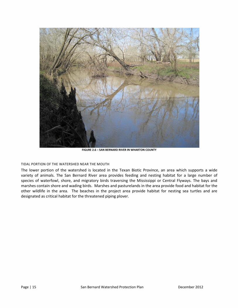
FIGURE 2.6 – SAN BERNARD RIVER IN WHARTON COUNTY
TIDAL PORTION OF THE WATERSHED NEAR THE MOUTH
The lower portion of the watershed is located in the Texan Biotic Province, an area which supports a wide variety of animals. The San Bernard River area provides feeding and nesting habitat for a large number of species of waterfowl, shore, and migratory birds traversing the Mississippi or Central Flyways. The bays and marshes contain shore and wading birds. Marshes and pasturelands in the area provide food and habitat for the other wildlife in the area. The beaches in the project area provide habitat for nesting sea turtles and are designated as critical habitat for the threatened piping plover.

Page | 16 San Bernard Watershed Protection Plan December 2012
FIGURE 2.7 – SAN BERNARD RIVER IN BRAZORIA COUNTY NEAR THE MOUTH
LAND COVER AND POPULATION CHARACTERISTICS
LAND COVER AND LAND COVER
Much of the land throughout the watershed is used for crop production and cattle grazing, and the river is used for boating and fishing. Today, small towns among vast open spaces, with no major metropolitan area, characterize the watershed. The major agribusiness types in the watershed are beef cattle grazing and hay production. The counties in the northern and west central portions of the San Bernard River watershed are among the top cattle/ calf producers in the state. Other common crops found throughout the watershed include rice, sorghum, corn, cotton, and soybeans. Land cover in the watershed is primarily rural and agricultural, with scattered areas of urbanization, in the lower part of the watershed there is a lot of barge traffic associated with the natural resource industry. Minerals are another major natural resource found within the area. Oil, gas, sulfur, and salt are abundant subsurface features. Petrochemical services are another facet of the economy. Of particular geological significance, Boling Dome is situated on the western bank of the San Bernard River, in the easternmost part of Wharton County, near Boling-Lago. This subsurface structure contains petroleum, sulfur, and salt. The associated sulfur reserve has produced more sulfur than any other mine in the world. As of 1990, 80.5 million tons of sulfur had been removed, along with over 6,000 million cubic feet of natural gas, and over 25,500,000 barrels of oil. (Basin Highlights Report, H-GAC)

Page | 17 San Bernard Watershed Protection Plan December 2012
Conoco-Phillips has a refinery located in Sweeny that contains a natural gas liquid processing center and petrochemical production facilities. The facility uses the river to transport tankers from the facility in Sweeny to the Port of Freeport. Products produced include gasoline, jet fuel, and diesel fuel.
TABLE 2.1- LAND COVER IN THE SAN BERNARD WATERSHED 2006
2006 National Land Cover Dataset
Acres Percent of Total
Developed 33,048 5.7%
Cultivated 209,198 35.8%
Grassland 185,863 31.8%
Forest 45,394 7.8%
Woody Wetland 84,292 14.4%
Herbaceous Wetland 21,344 3.7%
Bare 1,303 0.2%
Open Water 4,194 0.7%
TOTAL ACRES 584,634 100%
Much of the lower part of the watershed is wetlands and forest with residential uses along the waterways, the central part of the watershed is barren land and cultivated lands, and the upper part of the watershed is barren land and forest.
FIGURE 2.8 - LAND COVER IN THE SAN BERNARD WATERSHED 2006

Page | 18 San Bernard Watershed Protection Plan December 2012
EXISTING LAND MANAGEMENT PRACTICES
The Texas State Soil and Water Conservation Board has 152 Water Quality Management Plans in the San Bernard Watershed. These WQMPs are site-specific plans that are developed and approved by soil and water conservation districts to include appropriate land treatment practices, production practices, management measures, technologies or combinations of these. The purpose of these plans is to achieve water pollution prevention and to be consistent with state water quality standards. These plans do not cost anything to develop, but there are costs associated with implementation of practices to improve water quality, and there is financial assistance available. Types of plans that have already been implemented in the San Bernard Watershed include: prescribed grazing, nutrient management, crop residue management, irrigation water management, forage harvest management, and pest management. The acreage in the San Bernard Watershed under a water quality management plan is 64,383 acres and the total acreage is 680,435, so approximately 9% of the watershed is under a plan currently. Below is a table showing the percentage of acreage under each type of management measure.
TABLE 2.2 – EXISTING MANAGEMENT PRACTICES BY ACRES
Management Measure Acres Percent of Watershed
Prescribed Grazing 31,698 4.7%
Nutrient Management 46,444 6.8%
Crop Residue Management/ Conservation Crop Rotation
29,304 4.3%
Forage Harvest Management 2,846 0.4%
Wildlife Land 9,456 1.4%
POPULATION GROWTH
The household population growth was generated for the watershed by the H-GAC. Growth was forecast for
urban and rural areas over a thirty year period in 5 year increments. The total population of the watershed is
expected to more than double in the next thirty years. It is expected that the majority of the new population
growth will be in cultivated and grassland areas (80%) and in forest and wetland areas (20%). As the population
in the watershed grows, it is expected that bacteria concentrations associated with urban and residential uses
such as on-site sewage facilities and pets will continue to increase as rural sources like livestock sources will
decrease.
TABLE 2.3 – WATERSHED POPULATION BY DECADE
Year 2010 2015 2020 2025 2030 2035 2040
Total Population
19,588 20,927 23,594 27,174 32,518 39,207 45,746
BIOLOGY
A recent water quality and biological study conducted by the United States Geological Survey (USGS; East and Hogan, 2003) on the San Bernard River found that fish diversity and numbers decreased as they sampled down river. The study reports only seven species including longnose gar (Lepisosteus osseus), channel catfish (Ictalurus

Page | 19 San Bernard Watershed Protection Plan December 2012
punctatus), longear sunfish (Lepomis megalotis), freshwater drum (Aplodinotus grunniens), blackstripe topminnow (Fundulus notatus), blacktail shiner (Cyprinella venusta), and red shiner (Cyprinella lutrensis) from a collection station at West Columbia, approximately 25 miles upstream, from a list of 32 fish species found in the river at all sampling locations. With the near total closure of the mouth of the river and minimal flow or tidal exchange, it is assumed that the river supports a diverse fish population of more salt tolerant species.
GEOMORPHOLOGY
This very active coastal area has undergone significant change over the last 80 years, due in large part to impacts to coastal sediment budget resulting from the development of the Port of Freeport and the dredging of the Gulf Intercoastal Water Way. The diversion of the Brazos River for port development resulted in a significant increase in the amount of sediment transported southward to the San Bernard River area, while the GIWW provides a channel available to “capture” flow from the impeded river, further reducing the current necessary to keep the mouth of the river open. Apparently unaware of the 2002 ERDC report (Kraus, 2002), TPWD’s Coastal Fisheries Division evaluated the blockage of the river’s mouth in 2004 in an attempt to determine the potential impact of the GIWW on the lower river (Chen and Buzan, 2004). Although their study was inconclusive as to the influence of the GIWW on the river, Chen and Buzan document that the mouth migrated from its 1974 location (the approximate location proposed for its restoration in this project), over 1.3 miles to the southwest by 2002. The 1974 location of the river’s mouth is now blanketed by a substantial sand spit that was dredged through in this current restoration effort.
ADDITIONAL DATA NEEDED FOR FUTURE MODELING
Assumptions have been made regarding E. coli levels in effluent from WWTFs in the watershed. Currently we do
not have any data for these outfalls, so it is being assumed that they are releasing effluent that is within the
current standards. As WWTFs renew their permits they will be required to start reporting E. coli levels.
SOURCES OF INFORMATION
USGS in Cooperation with the Houston-Galveston Area Council and the Texas Commission on Environmental Quality; Hydrologic, Water-Quality, and Biological Data for Three Water Bodies, Texas Gulf Coastal Plain, 2000-2002; Open File Report 03-459 2008 Texas 303(d) List, March 19, 2008, Texas Commission on Environmental Quality US Army Corps of Engineers, Galveston District; Draft Environmental Assessment – Restoration of the Mouth of the San Bernard River to the Gulf of Mexico, Brazoria County, Texas, June 2008 Halff Associates, Inc; San Bernard Watershed Flood Protection Planning Study Final Report, July 15, 2009.

Page | 20 San Bernard Watershed Protection Plan December 2012
3 – PUBLIC PARTICIPATION
PUBLIC PARTICIPATION
Public education and outreach are essential to the implementation of a successful Watershed Protection Plan.
In addition to the physical BMPs to be implemented by landowners and jurisdictions in the watershed,
behavioral BMPs can be addressed by everyone in the watershed. Public Participation can include public
education workshops, distribution of educational materials, and participation in activities to improve water
quality.
PUBLIC PARTICIPATION LEAD AGENCY ROLES AND RESPONSIBILITIES
STAKEHOLDER FACILITATION
Stakeholder Group members have actively participated in the Watershed Protection Plan Process. Members have identified and presented insights, suggestions, and concerns from a community, environmental, or public interest perspective.
FIGURE 3.1 – SAN BERNARD STAKEHOLDER MEETING

Page | 21 San Bernard Watershed Protection Plan December 2012
PROJECT PARTNERS
PROJECT PARTNERS
H-GAC worked with TCEQ in the preparation of the Watershed Protection Plan. A number of cities and school districts are located in the watershed. There are also a number of state and local agencies that operate within the watershed.
PARTNERS LIST
Counties: Austin Brazoria Colorado Fort Bend Wharton Cities: Eagle Lake Wallis East Bernard Kendleton Needville Wharton West Columbia Sweeny Brazoria Jones Creek Wild Peach Village
School Districts: Belleville Sealy Columbus Rice Consolidated Kendleton Needville Brazos Lamar Consolidated Damon Sweeny Columbia-Brazoria Brazosport Boling East Bernard Wharton El Campo
WPP STAKEHOLDER GROUP
STAKEHOLDER GROUP STRUCTURE
The Stakeholder Group was divided into committee members with voting privileges and at large stakeholder group members who will participate as available. Committee members will ultimately be responsible for plan implementation in the watershed.
GROUP MEMBERSHIP Voting Committee Members:
Commissioner Dude Payne (Brazoria County)
Nancy and Fred Kanter (FOR)
John Phillips (Waters Davis SWCD)
Jeremy Jett (Industry/Walmart, Sealy)
Darrell Schwebel (Cradle of Texas Conservancy/DOW)
Carol Jones (homeowner)
Roy and Jan Edwards (homeowners, Rivers End)
Linda and Ken Wright (FOR)
William Todd (Ag producer)
Page | 22 San Bernard Watershed Protection Plan December 2012
Sheri and Melvin Ganske (Boling property owners)
Richard Forgason (ag, Hungerford)
Harry Anderson (ag, East Bernard)
Terry Hlavinka (Ag, East Bernard)
At Large Stakeholder Group Members:
Bill and Jackie Benson (homeowners)
Valroy and Adalia Maudlin (homeowners)
Greg Roque (business/industry, Sealy)
Karen Carroll (Brazoria Co. Health)
Charles Boettcher (Ag, East Bernard)
Harry Goudeau (Ag, Hungerford)
John Wallace (landowner, Brazoria)
Michael Lange (FWS)
Paul Wood (engineer)

Page | 23 San Bernard Watershed Protection Plan December 2012
SUBCOMMITTEES AND WORKGROUPS In order to carry out its responsibilities, the Stakeholder Group has discretion to form standing and ad hoc work groups to carry out specific assignments from the group.
ROLES AND RESPONSIBILITIES Stakeholder group members assisted with:
Site visits, photos, sample site descriptions Advertising the plan Provide/gather information on issues and concerns of the watershed Knowledge of existing programs or plans to consider or integrate Technical assistance in developing and implementing the plan Responsible for implementation and communication to other affected parties Provide review and comments on plan as it is written.
AGENCIES INVOLVED AS STAKEHOLDERS
Texas Commission on Environmental Quality Texas Parks and Wildlife U.S. Fish and Wildlife United States Army Corps of Engineers Texas State Soil and Water Conservation Board (TSSWCB) Soil and Water Conservation Districts (SWCD) Extension Agents – Ag and Natural Resources District Conservationists US Department of Agriculture (USDA)
CITIZENS INVOLVED AS STAKEHOLDERS
Friends of the River - San Bernard is a very active citizen group involved in the watershed. The group is currently organized into committees based on their interests and professional affiliations.
GOALS DEVELOPMENT
Stakeholder group members assisted with the goals and visioning of the project, and identified and prioritize programs and practices to achieve these goals. The stakeholder committee members are ultimately responsible for the implementation of projects to achieve these goals.
SELECTION OF THE LEAD ORGANIZATION FOR IMPLEMENTATION/UPDATE OF THE WPP
Friends of the River San Bernard, Stream Team members, and local Master Naturalists are currently doing a lot of work to help advance the Watershed Protection Plan through public education and outreach measures. The Texas State Soil and Water Conservation board is also advertising farm plans to property owners in the watershed. Counties and other authorized agents are updating and strengthening the OSSF regulation and permitting efforts.

Page | 24 San Bernard Watershed Protection Plan December 2012
4 - WATERSHED ANALYSIS
HYDROLOGY
The San Bernard River Watershed drains approximately 900 square miles, the river flows southeast to form the boundary between Austin and Colorado counties, then flows between Wharton and Fort Bend County and through Brazoria County before emptying into the Gulf of Mexico. The San Bernard River comprises two stream segments defined by TCEQ. Stream segment 1302 is the San Bernard River Above-Tidal, which flows from the city of New Ulm in Austin County to a point 2.0 mi upstream of State Highway 35 in Brazoria County. Stream segment 1301 is San Bernard River Tidal, which flows from 2.0 mi upstream of State Highway 35 in Brazoria County to the Gulf of Mexico. There are concerns about dissolved oxygen levels and nutrients, and the river is listed as impaired for bacteria on the 303d list.
FIGURE 4.1 – AERIAL PHOTO OF SAN BERNARD RIVER MOUTH IN 2010
In the upper portions of the watershed, the river has had minimal flow for most of the year over the past 20 years, however there used to be a more significant flow. A number of factors have contributed to the lack of flow, including recent drought, creation of retention ponds, more impervious surfaces which reduce inflow, and increased vegetation and tree cover along the river banks. The recent drought has caused a number of issues for the watershed, including limited flow in the non-tidal part of the watershed, increased salinity, changes in biological composition, and lower dissolved oxygen. The drought has also resulted in several drought related problems such as fish kills and an occurrence of red tide along the coast. The past few years have not been representative of usual watershed conditions. The period of analysis for the watershed modeling was 2007-2009 when data was available. The tidal and non-tidal portions of the watershed are separated by the salt barrier dam. This small dam is located on the river near West Columbia about one mile north of Highway 35. The purpose of the dam is to prevent saltwater from the Gulf from reaching the upper portions of the river that are used for

Page | 25 San Bernard Watershed Protection Plan December 2012
water supply for industrial uses. There is also a diversion area on the Wharton-Fort Bend County line called the New Gulf Reservoir, it is owned by the Texas Gulf Sulfur Company and is used for municipal supply and irrigation. The mouth of the San Bernard River has migrated about two miles to the southwest since the 1929 construction of the Diversion Channel and the 1940 construction of the Gulf Intercoastal Water Way (GIWW), and almost closed at the Gulf of Mexico due to sand accretion from the delta formed by the Diversion Channel. Accretion has accelerated over the last ten years due to a number of factors, including flooding on the Brazos River. The result of the sediment buildup caused the river discharge to not be sufficient enough to flush the shoaling at the mouth of the river and keep it open to the Gulf. The blockage of the river’s mouth diverted flow into the GIWW, raising concerns for barge traffic along the GIWW (Kraus, 2002). The Galveston District, USACE, has received reports that barge tows traveling along the GIWW between the San Bernard and Brazos Rivers can experience an eastward flowing current that is sufficiently strong to pose a potential navigation hazard. To allow for a more effective, safe, and efficient waterway, the proposed restoration of the mouth of the San Bernard River would reduce treacherous currents resulting from diverted flow into the GIWW and Brazos River Floodgates. In 2002, a study by the U.S. Army Engineer Research and Development Center (ERDC) addressed how to improve navigation safety and efficiency on the GIWW in the vicinity of the San Bernard River. The purpose of the project was to reconnect the San Bernard River with the Gulf of Mexico at its historic location. The conclusion of the study was that dredging a shorter, deeper channel to the Gulf would increase the hydraulic efficiency of the river sufficiently to keep the mouth open and flowing for perhaps 6 to 12 years, before longshore transport of sediment from the Brazos River would again overtake the channel. Unfortunately, due to the severe drought in 2012, the river mouth has once again closed as of December 2012.
FIGURE 4.3 - HYDROGRAPH OF DAILY MEAN DISCHARGE AND TIME OF WATER-QUALITY SAMPLING ON SAN BERNARD NEAR BOLING, JULY
2000 - SEPTEMBER 2002 (USGS STUDY)
Page | 26 San Bernard Watershed Protection Plan December 2012
WATERBODY AND WATERSHED CONDITIONS
WATER QUALITY SAMPLING
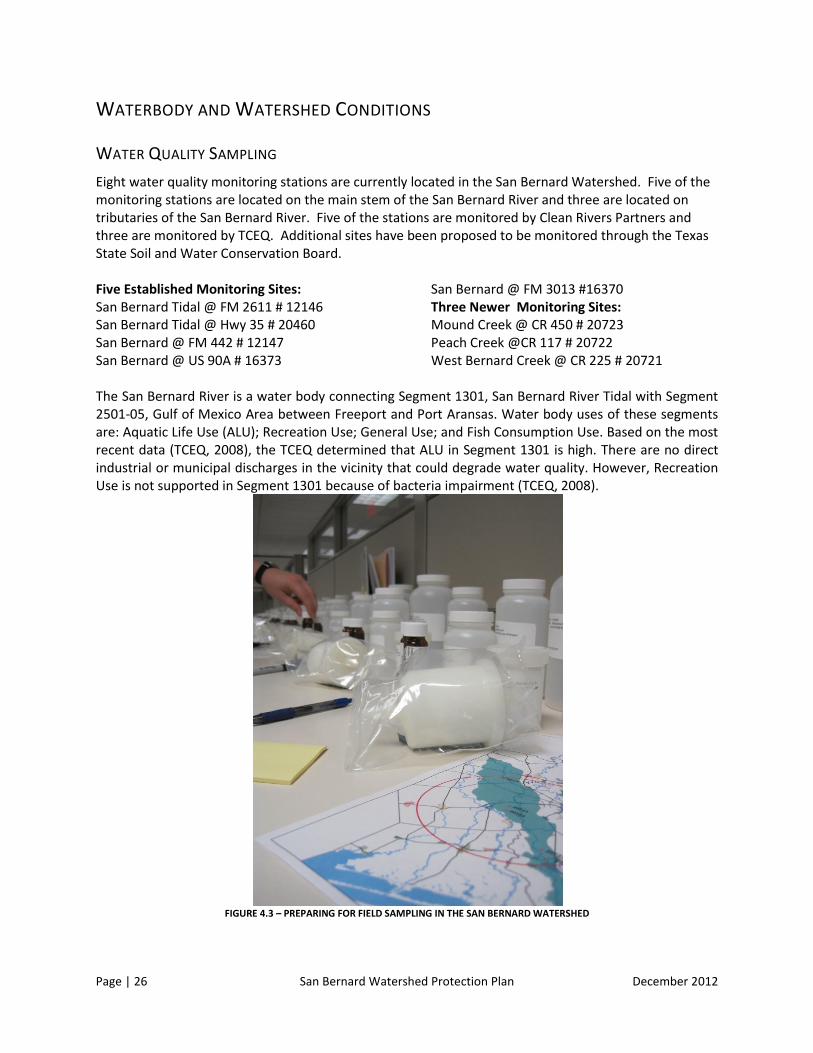
Eight water quality monitoring stations are currently located in the San Bernard Watershed. Five of the monitoring stations are located on the main stem of the San Bernard River and three are located on tributaries of the San Bernard River. Five of the stations are monitored by Clean Rivers Partners and three are monitored by TCEQ. Additional sites have been proposed to be monitored through the Texas State Soil and Water Conservation Board. Five Established Monitoring Sites: San Bernard Tidal @ FM 2611 # 12146 San Bernard Tidal @ Hwy 35 # 20460 San Bernard @ FM 442 # 12147 San Bernard @ US 90A # 16373
San Bernard @ FM 3013 #16370 Three Newer Monitoring Sites: Mound Creek @ CR 450 # 20723 Peach Creek @CR 117 # 20722 West Bernard Creek @ CR 225 # 20721
The San Bernard River is a water body connecting Segment 1301, San Bernard River Tidal with Segment 2501-05, Gulf of Mexico Area between Freeport and Port Aransas. Water body uses of these segments are: Aquatic Life Use (ALU); Recreation Use; General Use; and Fish Consumption Use. Based on the most recent data (TCEQ, 2008), the TCEQ determined that ALU in Segment 1301 is high. There are no direct industrial or municipal discharges in the vicinity that could degrade water quality. However, Recreation Use is not supported in Segment 1301 because of bacteria impairment (TCEQ, 2008).
FIGURE 4.3 – PREPARING FOR FIELD SAMPLING IN THE SAN BERNARD WATERSHED

Page | 27 San Bernard Watershed Protection Plan December 2012
A data study was completed by USGS in 2002, and data collection at six stations began in late summer of 2000. One monitoring meter was installed in the non-tidal portion of the watershed to collect data continuously (every thirty minutes). This allowed scientists to monitor the levels of dissolved oxygen under varying conditions. Other parameters collected included pH, conductivity, and temperature. Additional water quality monitoring sites were sampled monthly and included the parameters listed above as well as Biological Oxygen Demand, nitrogen and phosphorus compounds, dissolved solids, bacteria, and flow. Recordings from a permanent USGS station near Boling supplied continuous flow measurements. (USGS Study) Habitat and biological data collected along the San Bernard River and its tributaries have been summarized and compared with similar data from other streams in southeast Texas. Measures of stream habitat compare closely with other riverine settings, as opposed to tidally influenced, coastal bayous. Similarly, measures of aquatic insect and fish population diversity are similar to water bodies with minimally impacted watersheds. Based on these biological data, along with selected water chemistry and water-quality data that were also collected during 2000-2002, the San Bernard River does not exhibit significant water quality problems. The river has been removed from the list of water bodies not meeting designated standards for high aquatic life use due to low dissolved oxygen concentrations.
FIGURE 4.4 – WATER QUALITY MONITORING IN THE SAN BERNARD RIVER WATERSHED

Page | 28 San Bernard Watershed Protection Plan December 2012
303(D) LIST
From the 2008 303d list:

Page | 29 San Bernard Watershed Protection Plan December 2012
POLLUTANT SOURCES
POINT SOURCES
Point source pollution comes from known sources such as outfalls that flow into the river. Along the San
Bernard River, there are 6 industrial outfalls and 17 domestic outfalls from sources such as cities and schools.
There are a total of 23 known outfalls into the San Bernard.
NONPOINT SOURCES
Nonpoint source pollution is the combination of all other sources that are carried into the river as water runs
across the land and into the waterways. Common sources of nonpoint source pollution include: malfunctioning
septic systems, construction site runoff, agricultural sources, and runoff from streets and yards. Bacteria is the
primary cause of water quality problems in the San Bernard River. Possible sources of bacteria include: humans,
livestock, domestic animals, and other wildlife and non-domestic animals. Other sources of pollution include
nutrients, sediment, and toxic and hazardous substances.
BACTERIA Portions of the San Bernard River do not meet standards for contact recreation due to elevated levels of
bacteria. In the San Bernard watershed, bacteria levels average just over 126 and maximum levels are in the
400s. Although these numbers are higher than acceptable levels, they are not exceedingly high and can be
managed to reach acceptable levels. Following are a table and a chart of bacteria levels for 5 monitoring
stations along the San Bernard River and mean E. Coli and enterococci by year for stations in the tidal and non-
tidal parts of the watershed. In the tidal portion of the river the criteria is for enterococcus and the above tidal
criteria is for E. coli.

Page | 30 San Bernard Watershed Protection Plan December 2012
TABLE 4.1 - BACTERIA LEVELS FOR SAN BERNARD WATERSHED MONITORING STATIONS
FIGURE 4.5 – AVERAGE E.COLI AND ENTEROCOCUS DENSITY
Station Criteria
Min Max Average
16370 126 10 413 99
16373 126 30 369 168
12147 126 41 243 135
20460 35 1 201 64
12146 35 0 86 46
0
100
200
300
400
500
600
700
800
900
1000
16370 16373 12147 20460 12146
Bac
teri
al D
en
sity
(M
PN
/10
0 m
L)
Monitoring Station
Average E. Coli and Enterococus Density By Monitoring Station
E. Coli
Enterococcus Downstream

Page | 31 San Bernard Watershed Protection Plan December 2012
FIGURE 4.6 – E. COLI GEOMETRIC MEAN BY YEAR
FIGURE 4.7 – ENTEROCOCI GEOMETRIC MEAN BY YEAR
0
200
400
600
800
1000
1200
2001 2002 2003 2004 2005 2006 2007 2008 2009 2010 2011
Ge
om
etr
ic M
ean
, MP
N/1
00
mL
E. Coli Geometric Mean By Year (MPN/100 mL)
Station 12147
Station 16373
Station 16370
0
50
100
150
200
250
2001 2002 2003 2004 2005 2006 2007 2008 2009 2010 2011
Ge
om
etr
ic M
ean
, MP
N/1
00
mL
Enterococci Geometric Mean By Year (MPN/100 mL)
Station 12146
Station 20460

Page | 32 San Bernard Watershed Protection Plan December 2012
NUTRIENTS
In addition to high levels of bacteria, there are also higher levels of nutrients found in the San Bernard River.
Maximum nutrient levels allowed in a stream or river are <1.95 mg/L nitrate nitrogen and <0.69 mg/L total
phosphorous. Both nitrogen and phosphorous are found in the natural environment, but they are also found in
fertilizers added by humans. They are necessary for plant growth, but at high levels they can cause overgrowth
of plants. Below are five tables of nutrient mean concentrations by year for nitrate+nitrogen, total phosphorus,
orthophosphate, ammonia, and average mean by year.
FIGURE 4.8 - NITRATE + NITRITE, AS NITROGEN MEAN BY YEAR, 1987 - PRESENT
0
0.2
0.4
0.6
0.8
1
1.2
1.4
1.6
Me
an C
on
cen
trat
ion
, mg/
L
Nitrate -Nitrogen Mean Concentration By Year (mg/L)
Station 12147 Station 12146 Station 16373 Station 16370 Station 20460

Page | 33 San Bernard Watershed Protection Plan December 2012
Figure 4.9 – Total Phosphorus Mean Concentration By Year
Figure 4.10 – Orthophosphate –P Mean Concentration By Year
0
0.2
0.4
0.6
0.8
1
1.2
Me
an C
on
cen
trat
ion
(m
g/L)
Total Phosphorus Mean Concentration By Year (mg/L)
Station 12147
Station 12146
Station 16373
Station 16370
0
0.1
0.2
0.3
0.4
0.5
0.6
Me
an C
on
cen
trat
ion
(m
g/L)
Orthophosphate-P Mean Concentration By Year (mg/L)
Station 12147
Station 12146
Station 16373
Station 16370

Page | 34 San Bernard Watershed Protection Plan December 2012
Figure 4.11 – Ammonia Mean Concentration By Year
FIGURE 4.12 - AVERAGE NUTRIENT CONCENTRATION BY MONITORING STATION
0
0.2
0.4
0.6
0.8
1
1.2
19
70
19
73
19
75
19
77
19
79
19
81
19
83
19
85
19
87
19
89
19
91
19
93
19
95
19
97
19
99
20
01
20
03
20
05
20
07
20
09
20
11
Me
an C
on
cen
trat
ion
, mg/
L
Ammonia Mean Concentration By Year (mg/L)
Station 12147
Station 12146
Station 16373
Station 16370
Station 20460
-0.10
0.00
0.10
0.20
0.30
0.40
0.50
0.60
0.70
16370 16373 12147 20460 12146
Nu
trie
nt
Co
nce
ntr
atio
n, m
g/L
Monitoring Station
Average Nutrient Concentration By Monitoring Station 2003 - 2008
Ammonia-N
Nitrate+Nitrite - N
Orthophosphate -P
Total Phosphate-P
Downstream
Page | 35 San Bernard Watershed Protection Plan December 2012
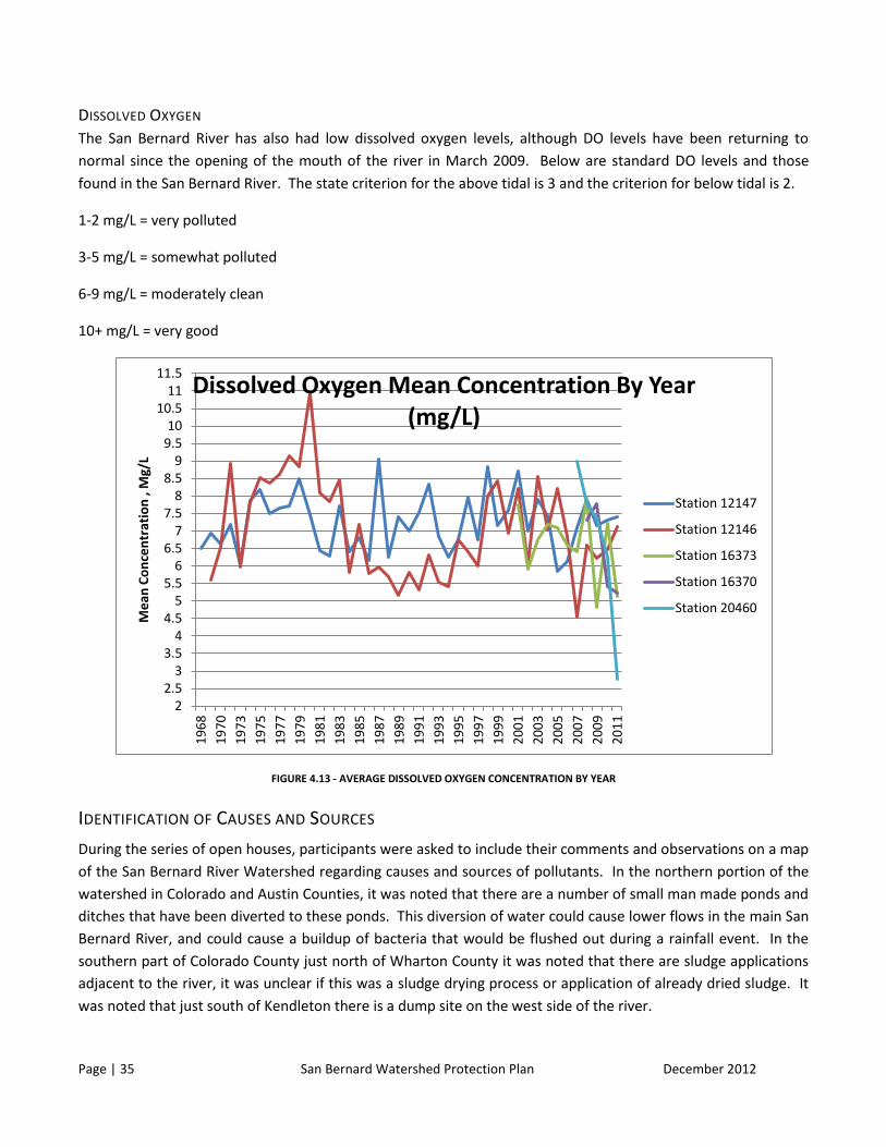
DISSOLVED OXYGEN
The San Bernard River has also had low dissolved oxygen levels, although DO levels have been returning to
normal since the opening of the mouth of the river in March 2009. Below are standard DO levels and those
found in the San Bernard River. The state criterion for the above tidal is 3 and the criterion for below tidal is 2.
1-2 mg/L = very polluted
3-5 mg/L = somewhat polluted
6-9 mg/L = moderately clean
10+ mg/L = very good
FIGURE 4.13 - AVERAGE DISSOLVED OXYGEN CONCENTRATION BY YEAR
IDENTIFICATION OF CAUSES AND SOURCES
During the series of open houses, participants were asked to include their comments and observations on a map
of the San Bernard River Watershed regarding causes and sources of pollutants. In the northern portion of the
watershed in Colorado and Austin Counties, it was noted that there are a number of small man made ponds and
ditches that have been diverted to these ponds. This diversion of water could cause lower flows in the main San
Bernard River, and could cause a buildup of bacteria that would be flushed out during a rainfall event. In the
southern part of Colorado County just north of Wharton County it was noted that there are sludge applications
adjacent to the river, it was unclear if this was a sludge drying process or application of already dried sludge. It
was noted that just south of Kendleton there is a dump site on the west side of the river.
2 2.5
3 3.5
4 4.5
5 5.5
6 6.5
7 7.5
8 8.5
9 9.5 10
10.5 11
11.5
19
68
19
70
19
73
19
75
19
77
19
79
19
81
19
83
19
85
19
87
19
89
19
91
19
93
19
95
19
97
19
99
20
01
20
03
20
05
20
07
20
09
20
11
Me
an C
on
cen
trat
ion
, M
g/L
Dissolved Oxygen Mean Concentration By Year (mg/L)
Station 12147
Station 12146
Station 16373
Station 16370
Station 20460
Page | 36 San Bernard Watershed Protection Plan December 2012
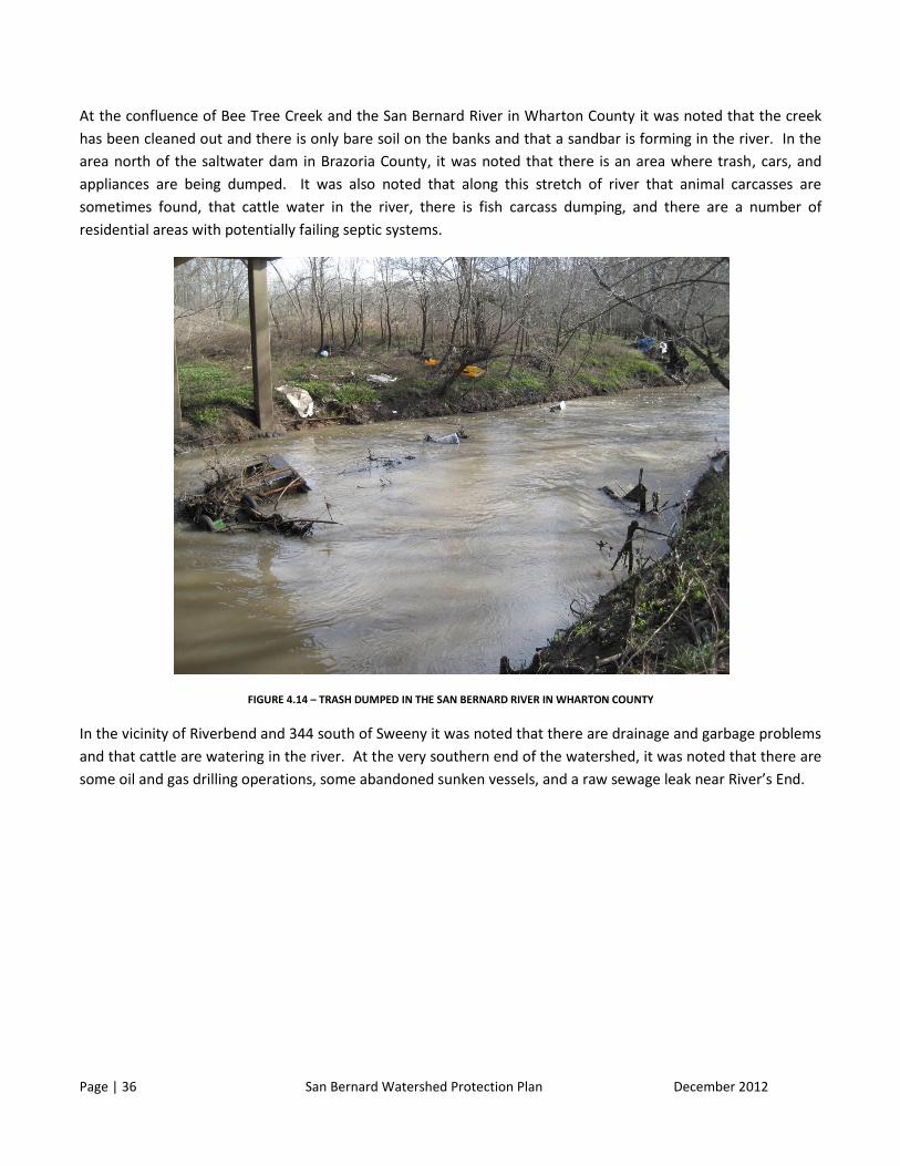
At the confluence of Bee Tree Creek and the San Bernard River in Wharton County it was noted that the creek
has been cleaned out and there is only bare soil on the banks and that a sandbar is forming in the river. In the
area north of the saltwater dam in Brazoria County, it was noted that there is an area where trash, cars, and
appliances are being dumped. It was also noted that along this stretch of river that animal carcasses are
sometimes found, that cattle water in the river, there is fish carcass dumping, and there are a number of
residential areas with potentially failing septic systems.
FIGURE 4.14 – TRASH DUMPED IN THE SAN BERNARD RIVER IN WHARTON COUNTY
In the vicinity of Riverbend and 344 south of Sweeny it was noted that there are drainage and garbage problems
and that cattle are watering in the river. At the very southern end of the watershed, it was noted that there are
some oil and gas drilling operations, some abandoned sunken vessels, and a raw sewage leak near River’s End.

Page | 37 San Bernard Watershed Protection Plan December 2012
FIGURE 4.15 – POTENTIAL CAUSES AND SOURCES OF POLLUTION IN THE SAN BERNARD WATERSHED
At this time, all causes and sources of the pollutants are unknown, but information received from stakeholders
and public meetings have helped further identify areas that may be sources of bacteria to the San Bernard River.
Additional monitoring will be implemented to further identify causes and sources of pollutants, and once
identified; BMPs will be applied to lessen the amount of pollutants being carried into the San Bernard River.
An online survey was also conducted of watershed residents and landowners; the response rate was about 10%.
Questions included asking respondents how they use their land in the watershed, how much land they have, and
whether or not they have been involved in the Watershed Protection Plan Process. The respondents were asked
to specify which BMPs they thought would best address the identified causes and sources of pollution.
Respondents also had the opportunity to answer some open ended questions about what they thought needed
to be added to the plan, what the biggest obstacle in implementing the plan would be, and were given the
opportunity to add any other additional comments. The following causes and sources of pollutants in the San
Bernard Watershed were identified.

Page | 38 San Bernard Watershed Protection Plan December 2012
FIGURE 4.16 – STAKEHOLDER PRIORITIZATION OF CAUSES AND SOURCES OF POLLUTION IN THE SAN BERNARD WATERSHED
WATER QUALITY AND FLOW
H-GAC has been monitoring water quality and flow in the San Bernard watershed for an extended period of time, below is a
snapshot of the sampling results for the eight sites currently being sampled.
TABLE 4.2 - WATER QUALITY MONITORING DATA
Monitoring Station
Parameter Number
of Samples
Minimum Maximum Mean Sampling
Period
12146 Ammonia-N 169 0.01 1.9 0.14 1969-2010
Dissolved Oxygen 180 2.9 18.1 7.5 1969-2010
Enterococci 37 5 10462 385 1969-2010
Nitrate-N 189 0.01 2.12 0.28 1969-2010
Orthophosphate-P 147 0.02 1.66 0.18 1969-2010
pH 138 6.5 9.9 7.7 1969-2010
Total Phosphorus 166 0.01 6.18 0.29 1969-2010
Total Suspended
Solids 170 2 359 38 1969-2010
12147 Ammonia-N 165 0 3 0.14 1970-2011
Dissolved Oxygen 188 3.8 12.5 7.3 1968-2011
E. Coli 44 10 9804 765 2001-2011
Nitrate-N 187 0.01 3.26 0.43 1970-2011

Page | 39 San Bernard Watershed Protection Plan December 2012
Orthophosphate-P 143 0.03 1.44 0.18 1973-2011
pH 124 6.2 8.8 7.6 1973-2010
Total Phosphorus 159 0.07 4.18 0.27 1970-2011
Total Suspended
Solids 162 1 320 61 1970-2011
16370 Ammonia-N 13 0.05 0.05 0.05 2007-2010
Dissolved Oxygen 12 3.8 9.4 6.6 2007-2010
E. Coli 13 10 2000 257 2007-2010
Nitrate-N 13 0.02 0.02 0.02 2007-2010
Orthophosphate-P 13 0.02 0.05 0.02 2007-2010
pH 12 6.9 7.9 7.5 2007-2010
Total Phosphorus 13 0.03 0.41 0.12 2007-2010
Total Suspended
Solids 13 1 18 6 2007-2010
16373 Ammonia-N 35 0.03 0.3 0.07 2001-2010
Dissolved Oxygen 40 4.1 10.9 6.8 2001-2010
E. Coli 37 62 3076 388 2001-2010
Nitrate-N 37 0.02 1.17 0.29 2001-2010
Orthophosphate-P 35 0.02 0.26 0.13 2001-2010
pH 41 6.4 8 7.5 2001-2010
Total Phosphorus 36 0.03 0.49 0.22 2001-2010
Total Suspended Solids
34 2 109 33 2001-2010
20460 Ammonia-N 12 0.05 0.6 0.1 2007-2010
Dissolved Oxygen 13 3.8 11.1 7.4 2007-2010
Enterococci 12 5 410 116 2007-2010
Nitrate-N 12 0.02 2.33 0.22 2007-2010
Orthophosphate-P 12 0.02 0.27 0.15 2007-2010
pH 13 7.5 8.3 7.8 2007-2010
Total Phosphorus 12 0.09 0.94 0.33 2007-2010
Total Suspended
Solids 12 4 85 22 2007-2010
20721 Ammonia-N 5 0.05 0.2 0.08 2010
Dissolved Oxygen 5 4.3 9.6 5.8 2010
E. Coli 5 41 170 96 2010
Nitrate-N 5 0.02 0.37 0.24 2010
Orthophosphate-P 5 0.09 0.23 0.16 2010
pH 5 7.3 7.5 7.5 2010
Total Phosphorus 5 0.22 0.49 0.35 2010
Total Suspended
Solids 5 11 84 44 2010
20722 Ammonia-N 5 0.05 0.05 0.05 2010
Dissolved Oxygen 5 3.4 8.8 5.1 2010
E. Coli 5 31 290 135 2010
Nitrate-N 5 0.02 0.16 0.11 2010
Orthophosphate-P 5 0.19 0.41 0.27 2010

Page | 40 San Bernard Watershed Protection Plan December 2012
pH 5 7.4 7.5 7.4 2010
Total Phosphorus 5 0.23 0.56 0.37 2010
Total Suspended
Solids 5 8 49 26 2010
20723 Ammonia-N 5 0.05 0.05 0.05 2010
Dissolved Oxygen 5 1.3 10.2 4.4 2010
E. Coli 3 5 150 62 2010
Enterococci 2 120 1300 710 2010
Nitrate-N 5 0.02 0.07 0.04 2010
Orthophosphate-P 5 0.11 0.3 0.16 2010
pH 5 7.3 7.9 7.7 2010
Total Phosphorus 5 0.17 0.42 0.27 2010
Total Suspended
Solids 5 3 101 31 2010
TABLE 2.3 - SAN BERNARD RIVER AND TRIBUTARIES MONITORING STATIONS (USGS STUDY)
Station Number Station Name Drainage Area (sq
mi)
Population Density (people per sq mi)
Data Collection Activity
294036096165001 Coushatta Creek at Attwater
Prairie Chicken NWR 39.9
10
Bimonthly water-quality sampling/ Biological
sampling
293211096110301 West Bernard Creek at CR 252 22.1 39 Bimonthly water-quality
sampling/ Biological sampling
293123096073001 Gum Tree Branch at CR 252 35.1 29 Bimonthly water-quality
sampling/ Biological sampling
292939096014001 San Bernard River at FM 2919 375 24 Bimonthly water-quality
sampling/ Biological sampling
08117500 San Bernard River near Boling 727 30
Continuous stream flow/ Continuous water-quality
monitoring/ Bimonthly water-quality sampling/
Biological sampling
290935095455601 San Bernard River at FM 1301 825 32
Continuous stream flow/ Continuous water-quality
monitoring/ Bimonthly water-quality sampling/
Biological sampling
RAINFALL INFORMATION
Weather data for the simulation was collected from five weather stations in and around the San Bernard
Watershed: Brenham, Bellville, Wharton, Wharton Airport, and Freeport. Specific information on each type of
weather data is provided in more detail subsequently.

Page | 41 San Bernard Watershed Protection Plan December 2012
Although precipitation data were collected from the five stations noted previously, three stations (Bellville,
Wharton, and Freeport) are located closest to the watershed. Therefore, data from these three stations were
used preferentially to generate most of the precipitation input for SWAT. If there were gaps in the data during
the simulation period the other two stations were used to complete these gaps.
SOURCES OF INFORMATION
USGS in Cooperation with the Houston-Galveston Area Council and the Texas Commission on Environmental Quality; Hydrologic, Water-Quality, and Biological Data for Three Water Bodies, Texas Gulf Coastal Plain, 2000-2002; Open File Report 03-459 2008 Texas 303(d) List, March 19, 2008, Texas Commission on Environmental Quality US Army Corps of Engineers, Galveston District; Draft Environmental Assessment – Restoration of the Mouth of the San Bernard River to the Gulf of Mexico, Brazoria County, Texas, June 2008 Halff Associates, Inc; San Bernard Watershed Flood Protection Planning Study Final Report, July 15, 2009.

Page | 42 San Bernard Watershed Protection Plan December 2012
5 - CAUSES AND SOURCES OF POLLUTION (ELEMENT A) Bacteria come from a number of sources throughout the watershed. Land uses and land cover vary widely
throughout the watershed from agriculture uses to urban uses. The upper portion of the watershed is more
rural in nature and not densely populated, the lower part of the watershed is more residential in nature. A
number of causes and sources of pollution have been identified by stakeholders throughout the watershed.
These sources include: domestic animals, trash and dumping, agriculture, industry, organic materials, OSSFs,
wildlife, and waste water treatment facilities. As the population in the watershed continues to grow, more land
in the watershed will be developed and subdivided, and potentially contribute to water quality problems. This
plan will identify prime sources through modeling and will identify BMPs to help reduce bacterial input into
waterways now and in the future.
MODELING APPROACH
The progression of steps in the WPP process includes quantification of sources, modeling of existing conditions,
and definition of reduction activities that will make an impaired stream meet state water quality standards
(USEPA, 1999). When a water body does not meet the standard required for its designated use, it is listed as
impaired on the Texas list of impaired waterways (303(d) list). These impairments are evaluated through the use
of bacterial indicators of pathogen contamination. The USEPA and the state of Texas have defined two types or
indicator organisms, Escherichia coli for freshwaters and Enterococci for marine waters.
The standards for these indicators depend on the assigned use of the stream: contact or non-contact recreation.
In Texas, there are two different levels of standards. The long-term trends in bacteria concentrations are
evaluated using the geometric mean standard. Instantaneous concentrations are evaluated using the single
sample, or the not-to-exceed standard.
San Bernard River and tributaries are classified as contact recreation water bodies; for this reason, the standards
currently used are E. coli geometric mean and single sample standard for the non-tidal portion and Enterococci
for tidal influenced streams. The E. coli 30-day geometric mean standard for contact recreation purposes is 126
cfu/dL and the single sample standard is 394 cfu/dL; while Enterococci standards are 35cfu/dL and 89cfu/dL
respectively.
For the regulatory Total Maximum Daily Load (TMDL) process addressing pathogen contamination, the EPA
published recommendations to assess E. coli source contribution and identification, characterize the sources,
and estimate the E. coli load produced by each source (USEPA, 2001). The EPA document recommends
identification of the location and densities of E. coli contributing source populations to characterize the loads in
a watershed. The same process is used for the modeling in San Bernard River watershed.
The Spatially Explicit Load Enrichment Calculation Tool (SELECT) was used in the development of the San
Bernard WPP to characterize the bacteria load associated to each individual source as well as the contribution of
each source within the watershed. The methodology followed in the application of the model was based on
Teague et al. (2009).
Page | 43 San Bernard Watershed Protection Plan December 2012
SWAT MODEL
The Soil and Water Assessment Tool (SWAT) was developed in the early 1990s at Texas A&M University by the
USDA Agricultural Research Service and is available in the public domain (Neitsch, Arnold et al. 2005). SWAT
focuses on runoff and loadings from rural and agriculture-dominated watersheds. Thus, SWAT is a continuous
model that simulates the effects of land management practices on water, sediment, and agricultural chemical
yields for large-scale complex watersheds or river basins.
A key advantage of SWAT is its extensive BMP evaluation module that simulates BMPs through several very
specific applications relevant to rural watersheds. The model can be used to evaluate operations that control
the plant growth cycle (i.e., planting and harvesting); application of fertilizer (both inorganic and manure),
grazing operations, use of grass filter strips and irrigation BMPs.
TIDAL PRISM MODELING
Tidal prism models (TPMs) are one-dimensional steady-state receiving water models that utilize the concept of
“tidal flushing” to simulate the physical transport of pollutants in a tidal basin over time. The theory of tidal
flushing was originally developed by Ketchum in 1951, and several TPMs have been developed and refined to
apply the concept towards water quality modeling of a variety of constituents, including bacteria (Kuo and
Neilson 1988; Kuo, Park et al. 2005; Shen, Sun et al. 2005).
TPMs perform simulations on a tidal cycle time scale, which is on the order of 12 hours depending on the
location. Data requirements are fairly low for TPMs compared to some other mechanistic receiving water
models, and as such they can only be used for smaller tidal basins and estuaries since one of the key
assumptions is that the tide rises and falls simultaneously throughout each modeled segment. Model
hydrodynamics are typically validated using a conservative tracer, such as salinity. Simple bacteria dynamics of
first order decay are generally assumed. Because no software has been developed for tidal prism model
development, models are generally programmed in Microsoft Excel, FORTRAN, or other programming
environments; as such, source code is generally available for the applications.
SELECT MODELING
SELECT was used to evaluate current and future (subsequent 30 years) bacteria loadings within the watershed.
In order to obtain more accurate results, the entire San Bernard watershed was divided up into 10
subwatersheds based on the HUC-12 division for Texas, their proximity to the biggest tributaries, and location of
water quality monitoring stations (Figure 5.1). Variables reflecting the percent land cover were calculated using
The National Land Cover Dataset (NLCD) from 2006. The land
TABLE 5.1 LAND COVER CATEGORIES BY SUBWATERSHED
Land Cover Category SUBW
1 SUBW 2
SUBW
3
SUBW
4 SUBW 5
SUBW
6
SUBW
7 SUBW 8 SUBW 9
SUBW
10
High Intensity Developed 0% 0% 0% 0% 0% 0% 0% 0% 1% 0%
Low Intensity Developed 1% 1% 1% 2% 2% 4% 1% 1% 5% 1%
Open Space Developed 0% 0% 0% 0% 0% 0% 0% 0% 2% 1%

Page | 44 San Bernard Watershed Protection Plan December 2012
Cultivated 62% 87% 89% 85% 77% 68% 47% 60% 26% 7%
Grassland/Shrub 12% 5% 6% 7% 6% 14% 9% 15% 27% 5%
Forest 20% 1% 2% 1% 1% 7% 1% 1% 6% 3%
Woody Wetland 4% 4% 2% 3% 12% 6% 38% 21% 27% 7%
Herbaceous Wetland 1% 1% 1% 1% 1% 1% 2% 1% 4% 70%
Bare 0% 0% 0% 0% 0% 0% 0% 0% 0% 0%
Open Water 0% 0% 0% 0% 0% 0% 1% 0% 2% 6%
FIGURE 5.1 SAN BERNARD WATERSHED SUBDIVISIONS

Page | 45 San Bernard Watershed Protection Plan December 2012
Information used to estimate bacterial loads for the subsequent 30 years were based on household forecast
information obtained from H-GAC. Housing and jobs forecasts were obtained for urbanized areas within the
watershed. These areas include: Beasley, Brazoria, Jones Creek, Kendleton, Needville, and Sweeny. The
additional number of estimated households for rural versus urban areas was also obtained for the 10
subwatersheds for the years 2010 to 2040. The total population in 2010 was estimated to be 18,520 and the
estimated population in 2040 is 44,006. The total rural population in 2010 was 10,144 and the urban population
was 8,376. In 2040 it is projected that the total rural population will be 33,059 and the urban population will be
10,974. However, it was necessary to make several assumptions in the projection of bacteria loadings. Although
the population will change, it was assumed that the type of housing remained the same, single family homes.
For growth of residential areas, an assumption that the new housing will be suburban single family homes on
1/2 acre lots. Additionally, land cover from pastures and farming was assumed to provide most of the area for
growth. Finally, the increased number of households in rural areas is assumed to be on OSSFs and those
projected to be in urban areas on WWTFs.
POTENTIAL SOURCES OF BACTERIA
Each source of E. coli was distributed to the appropriate subwatersheds and then bacteria loads were calculated.
The average daily load for each source was calculated according to the methodology suggested by EPA (USEPA,
2001); this is multiplying an individual species’ fecal coliforms (FC) excretion rate by the corresponding species
population. (Table 5.2) E. coli loads were assumed to be 50% of the Fecal coliform concentration (Teague et al.,
2009, Doyle and Erikson, 2006). E. coli sources were distributed to subwatersheds based on land cover
distribution and loadings associated with each of the land covers. Next, all different sources of bacteria
considered in the model are described.
TABLE 5.2 CALCULATIONS OF BACTERIA LOADINGS FOR THE PLANNING PERIOD
ALL CATEGORIES-Loading distribution
SOURCES 2011 2015 2020 2025 2030 2035 2040
OSSFs 9.0E+13 7.6E+13 8.3E+13 1.0E+14 1.3E+14 1.6E+14 1.9E+14
WWTFs 9.8E+09 1.0E+10 1.0E+10 1.1E+10 1.1E+10 1.2E+10 1.3E+10
Urban Runoff 5.9E+12 5.9E+12 5.9E+12 5.9E+12 6.0E+12 6.0E+12 6.0E+12
Dogs 3.7E+13 4.0E+13 4.5E+13 5.2E+13 6.2E+13 7.5E+13 8.8E+13
Livestock 1.1E+14 1.1E+14 1.1E+14 1.1E+14 1.1E+14 1.1E+14 1.1E+14
Wildlife 1.3E+13 1.3E+13 1.3E+13 1.3E+13 1.3E+13 1.3E+13 1.2E+13
TOTAL 2.6E+14 2.5E+14 2.6E+14 2.9E+14 3.2E+14 3.6E+14 4.0E+14
POINT SOURCES
WASTE WATER TREATMENT FACILITIES
Point sources of bacteria in the SELECT model originate from Waste Water Treatment Facilities’ (WWTF)
effluent. San Bernard River watershed accounts for a total of 19 WWTFs; but two of them present intermittent
flow, so no flow data is reported. Table 5.3 shows the permitted and self reported flow generated within each
subwatershed.

Page | 46 San Bernard Watershed Protection Plan December 2012
None of the WWTFS in the area are required to monitor for fecal contamination; however, two WWTFs reported
values of 126cfu/dL. For this reason, it was assumed that all WWTFs presented the same concentrations as the
ones reporting. Daily load from each WWTF is calculated by multiplying average self reported flow by bacteria
concentration (Table 5.3). Wastewater Treatment Facility loadings will rise slightly as the population in the
watershed increases, however they will not be a significant contribution to the total loading.
TABLE 5.3 SAN BERNARD WWTF EFFLUENTS
NON-POINT SOURCES
Non point sources are related to runoff and any other non-directly measurable source of contamination (on-site
facilities and deposition from wildlife and birds).
OSSFS
On-site sewage facilities (OSSFs) are another potential source of bacteria contamination. On-site sanitary
facilities are the predominant form of wastewater treatment for many areas of the watershed. These systems
are built to treat domestic wastewater where no sewer systems exist. Bacteria loading from these systems can
reach streams by overland flow from surface ponding during wet periods or through groundwater. When the
systems are properly designed and installed, they do not constitute a source of bacteria, but if they do not
receive proper maintenance, eventually they will fail. According to a study conducted by Reed, Stowe & Yanke
in 2001, regulated systems would have a failure rate of 12%, while unregulated systems would have a failure of
50%; OSSFs were regulated starting in 1989, while systems installed prior 1989 remain unregulated.
SUBWATERSHEDNumber Permitted Flow
(MGD)
Average Self Reported
Flow (MGD)1
SW1- SB/Little San Bernard River 1 0.050 0.001
SW2- SB/East Bernard Creek 2 0.595 0.159
SW4- West Bernard Creek 0 0.000 0.000
SW3- Middle Bernard Creek 2 0.110 0.040
SW1- SB/Snake Creek 6 1.058 0.444
SW6- Peach Creek 0 0.000 0.000
SW7- SB/Cedar Creek 1 0.400 0.181
SW8- Mound Creek 0 0.000 0.000
SW10- SB/Lower Tidal 5 2.282 1.250
SW9- SB/Upper Tidal 0 0.000 0.000
TOTAL 17 4.495 2.0761. From 01/2008

Page | 47 San Bernard Watershed Protection Plan December 2012
FIGURE 5.2 OSSF COVER
The number and location of households utilizing OSSFs was obtained from a recent database developed by H-
GAC. In cases where no installation year was available, it was assumed that 60% of the systems were
unregulated due to no installation date associated with them. The OSSF dataset is missing information for
Wharton and Colorado Counties, so the loadings are not very accurate for the watershed. Instead of using this
dataset, average household data was used to determine where population exists that is not connected to a
waste water treatment facility.
Next, the E. coli load for each subwatershed was calculated based on an estimated 70 gal/person/day discharge
and 5*106 cuf/dL E. coli concentrations (Table 5.2). The average number per household was obtained from the
2009 U.S Census (USCB 2009, Teague, 2009). The highest loadings from OSSFs are in the northeast part of the
watershed, and the lowest loadings are at the mouth of the water by the coast where there is little population.
Loadings from on-site sewage facilities will continue to increase as the population increases in the watershed,
however with proper installation and maintenance, these OSSFs will not contribute a significant portion of
bacteria loading to the watershed.
LIVESTOCK
Waste generated by range animals can be directly deposited into the stream or carried by runoff from fields to
the stream. Animal populations were obtained from the 2007 Census of Agriculture per each county (Table 5.4)
and the number of animals was uniformly distributed in 90% of Hay/Pasture and herbaceous areas; the density
of cattle per mile was calculated and assigned to specific land covers within each subwatershed. Then the
number of animals within each subwatershed was multiplied by the fecal coliform excretion rate and then
converted to E. coli load. (Table 5.2).

Page | 48 San Bernard Watershed Protection Plan December 2012
TABLE 5.4 NUMBER OF ANIMALS PER COUNTY (CENSUS OF AGRICULTURE - 2007)
NUMBER OF ANIMALS PER COUNTY
County Cattle Horses Sheep & Goats
Austin 70184 3491 1930
Brazoria 78560 5367 5481
Colorado 98283 1897 1036
Fort Bend 46206 3105 1258
Wharton 76780 1942 3591
Habitats for livestock were determined based on literature and previous studies (Table 5.4). Animal numbers
were distributed among the watersheds within each county based on land cover types.
TABLE 5.5 ASSIGNED HABITATS FOR WILDLIFE
Cattle Herbaceous + 90% of Hay Pasture areas
Horses Herbaceous + 90% of Hay Pasture areas
Sheep&Goats Herbaceous + 90% of Hay Pasture areas
FIGURE 5.3 CATTLE IN AUSTIN COUNTY
Bacteria loadings from livestock are expected to decrease over the next thirty years as more residential
development occurs in the watershed. The greatest loadings are in the south part of the watershed in the tidal
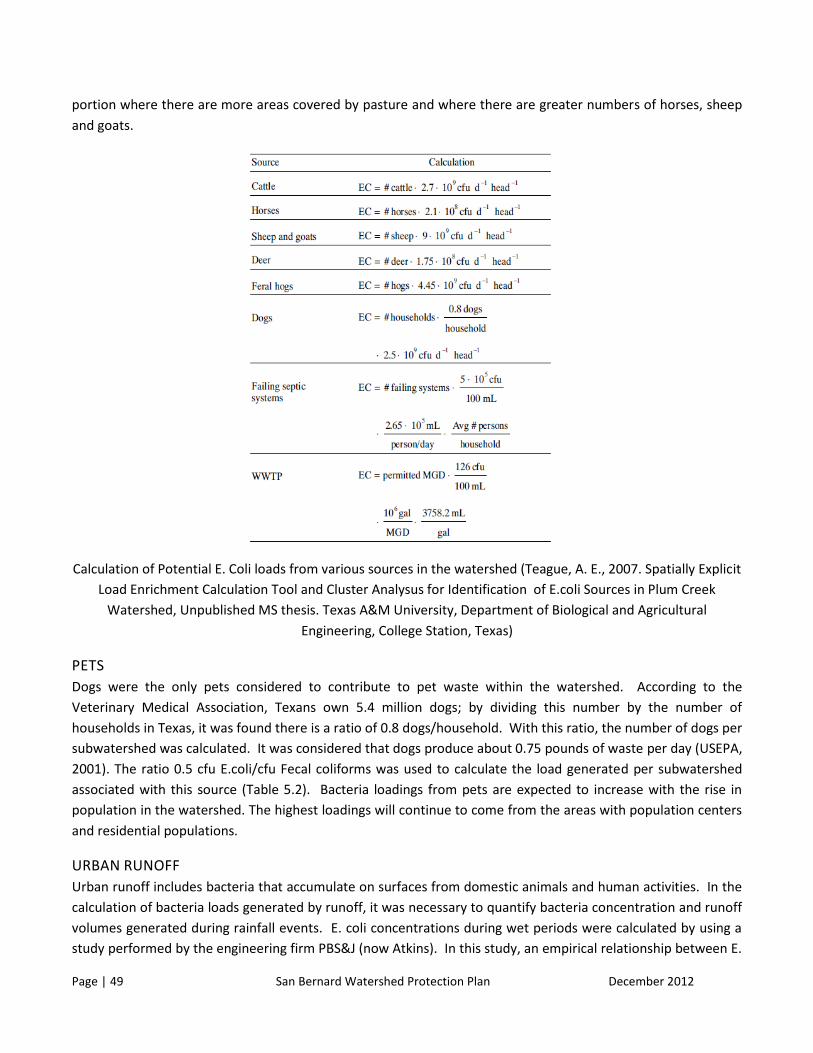
Page | 49 San Bernard Watershed Protection Plan December 2012
portion where there are more areas covered by pasture and where there are greater numbers of horses, sheep
and goats.
Calculation of Potential E. Coli loads from various sources in the watershed (Teague, A. E., 2007. Spatially Explicit
Load Enrichment Calculation Tool and Cluster Analysus for Identification of E.coli Sources in Plum Creek
Watershed, Unpublished MS thesis. Texas A&M University, Department of Biological and Agricultural
Engineering, College Station, Texas)
PETS
Dogs were the only pets considered to contribute to pet waste within the watershed. According to the
Veterinary Medical Association, Texans own 5.4 million dogs; by dividing this number by the number of
households in Texas, it was found there is a ratio of 0.8 dogs/household. With this ratio, the number of dogs per
subwatershed was calculated. It was considered that dogs produce about 0.75 pounds of waste per day (USEPA,
2001). The ratio 0.5 cfu E.coli/cfu Fecal coliforms was used to calculate the load generated per subwatershed
associated with this source (Table 5.2). Bacteria loadings from pets are expected to increase with the rise in
population in the watershed. The highest loadings will continue to come from the areas with population centers
and residential populations.
URBAN RUNOFF
Urban runoff includes bacteria that accumulate on surfaces from domestic animals and human activities. In the
calculation of bacteria loads generated by runoff, it was necessary to quantify bacteria concentration and runoff
volumes generated during rainfall events. E. coli concentrations during wet periods were calculated by using a
study performed by the engineering firm PBS&J (now Atkins). In this study, an empirical relationship between E.

Page | 50 San Bernard Watershed Protection Plan December 2012
coli concentrations and percentage of imperviousness was developed. The fraction of impervious cover
associated to each land cover was extracted from either a study conducted by the US EPA (Exum et al. 2005) or
guidance documents from the Tropical Storm Allison Recovery Project (TSARP). The simplest method was
applied to calculate Runoff volumes and E.coli loading within each subwatershed. Urban Runoff loadings are
associated to urban areas; for this reason, they are expected to increase as population and development
increase in the watershed.
SEWER SYSTEM OVERFLOWS (SSOS)
Sewer system overflow data was obtained for the entire San Bernard Watershed for the previous seven year
period. Seventy-one events were reported from four facilities during this time, 92% of which were generated by
storm events at one specific facility. Due to the discrete nature of the data, it was not included in the analysis.
TABLE 5.6 SEWER SYSTEM OVERFLOWS REPORTED IN SAN BERNARD WATERSHED
WILDLIFE
To estimate E. coli potential load generated by wildlife, deer, and feral hogs were considered the two major
contributors (Teague, 2009). Even if there are other wildlife sources such as birds, raccoons, coyotes and
opossums, they were not considered due to lack of reliable information.
Density population for deer was obtained from the Texas Parks and Wildlife Department (TPWD); deer densities
are reported for resource management units (RMUs). RMUs’ shapefile and densities were used to calculate
number of deer within each subwatershed. Then the fecal coliform excretion rate of 3.58*105 cfu/day-animal
(Zeckoski et al., 2005) was used to obtain the E. coli loads generated by this source within each subdivision.
Geese population data was received from Texas Parks and Wildlife for the San Bernard Watershed.
Stakeholders have identified waterfowl as a contributor to the bacteria loads in the watershed, however limited
data is available for bird populations.
Feral hog population range from 3.2 to 6 hogs/km2 in the Rio Grande Plains and lower coastal prairie of Texas
(Hellgren, 1997, Teague,2009). Loadings from feral hogs are distributed throughout the watershed since they
are found in all land covers and they reproduce rapidly. A density of 5 hogs/km2 was applied to the watershed
and then the number of animals was distributed in forested areas and scrublands. It was considered a fecal
coliform excretion rate of 4.45*109 cfu/animal. E. coli was again assumed to account for 50% of fecal coliform
concentration (Teague, 2009). The total loads per subwatershed were calculated (Table 5.2) and distributed per
subwatershed. As the population grows in the watershed, it is expected that the loading from wildlife may
decrease as habitat areas become more densely populated. Preferred habitats for wildlife were determined
based on literature and previous studies (Table 5.5). Animal numbers were distributed among the watersheds
within each county based on land cover types.
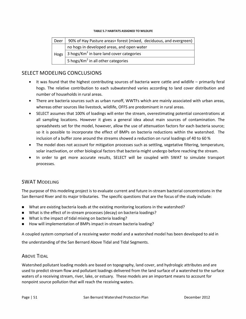
Page | 51 San Bernard Watershed Protection Plan December 2012
TABLE 5.7 HABITATS ASSIGNED TO WILDLIFE
Deer 90% of Hay Pasture areas+ forest (mixed, deciduous, and evergreen)
Hogs
no hogs in developed areas, and open water
3 hogs/Km2 in bare land cover categories
5 hogs/Km2 in all other categories
SELECT MODELING CONCLUSIONS
It was found that the highest contributing sources of bacteria were cattle and wildlife – primarily feral
hogs. The relative contribution to each subwatershed varies according to land cover distribution and
number of households in rural areas.
There are bacteria sources such as urban runoff, WWTFs which are mainly associated with urban areas,
whereas other sources like livestock, wildlife, OFFS are predominant in rural areas.
SELECT assumes that 100% of loadings will enter the stream, overestimating potential concentrations at
all sampling locations. However it gives a general idea about main sources of contamination. The
spreadsheets set for the model, however, allow the use of attenuation factors for each bacteria source;
so it is possible to incorporate the effect of BMPs on bacteria reductions within the watershed. The
inclusion of a buffer zone around the streams showed a reduction on rural loadings of 40 to 60 %
The model does not account for mitigation processes such as settling, vegetative filtering, temperature,
solar inactivation, or other biological factors that bacteria might undergo before reaching the stream.
In order to get more accurate results, SELECT will be coupled with SWAT to simulate transport
processes.
SWAT MODELING
The purpose of this modeling project is to evaluate current and future in-stream bacterial concentrations in the
San Bernard River and its major tributaries. The specific questions that are the focus of the study include:
What are existing bacteria loads at the existing monitoring locations in the watershed?
What is the effect of in-stream processes (decay) on bacteria loadings?
What is the impact of tidal mixing on bacteria loading?
How will implementation of BMPs impact in-stream bacteria loading?
A coupled system comprised of a receiving water model and a watershed model has been developed to aid in
the understanding of the San Bernard Above Tidal and Tidal Segments.
ABOVE TIDAL
Watershed pollutant loading models are based on topography, land cover, and hydrologic attributes and are
used to predict stream flow and pollutant loadings delivered from the land surface of a watershed to the surface
waters of a receiving stream, river, lake, or estuary. These models are an important means to account for
nonpoint source pollution that will reach the receiving waters.
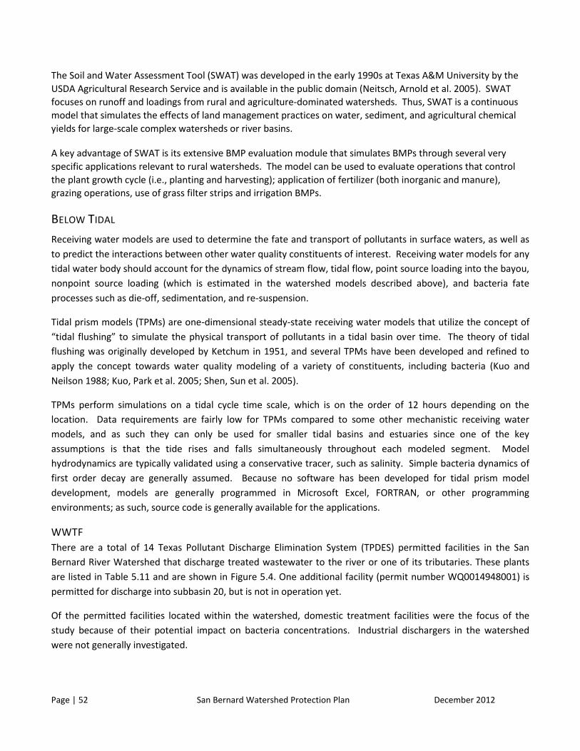
Page | 52 San Bernard Watershed Protection Plan December 2012
The Soil and Water Assessment Tool (SWAT) was developed in the early 1990s at Texas A&M University by the
USDA Agricultural Research Service and is available in the public domain (Neitsch, Arnold et al. 2005). SWAT
focuses on runoff and loadings from rural and agriculture-dominated watersheds. Thus, SWAT is a continuous
model that simulates the effects of land management practices on water, sediment, and agricultural chemical
yields for large-scale complex watersheds or river basins.
A key advantage of SWAT is its extensive BMP evaluation module that simulates BMPs through several very
specific applications relevant to rural watersheds. The model can be used to evaluate operations that control
the plant growth cycle (i.e., planting and harvesting); application of fertilizer (both inorganic and manure),
grazing operations, use of grass filter strips and irrigation BMPs.
BELOW TIDAL
Receiving water models are used to determine the fate and transport of pollutants in surface waters, as well as
to predict the interactions between other water quality constituents of interest. Receiving water models for any
tidal water body should account for the dynamics of stream flow, tidal flow, point source loading into the bayou,
nonpoint source loading (which is estimated in the watershed models described above), and bacteria fate
processes such as die-off, sedimentation, and re-suspension.
Tidal prism models (TPMs) are one-dimensional steady-state receiving water models that utilize the concept of
“tidal flushing” to simulate the physical transport of pollutants in a tidal basin over time. The theory of tidal
flushing was originally developed by Ketchum in 1951, and several TPMs have been developed and refined to
apply the concept towards water quality modeling of a variety of constituents, including bacteria (Kuo and
Neilson 1988; Kuo, Park et al. 2005; Shen, Sun et al. 2005).
TPMs perform simulations on a tidal cycle time scale, which is on the order of 12 hours depending on the
location. Data requirements are fairly low for TPMs compared to some other mechanistic receiving water
models, and as such they can only be used for smaller tidal basins and estuaries since one of the key
assumptions is that the tide rises and falls simultaneously throughout each modeled segment. Model
hydrodynamics are typically validated using a conservative tracer, such as salinity. Simple bacteria dynamics of
first order decay are generally assumed. Because no software has been developed for tidal prism model
development, models are generally programmed in Microsoft Excel, FORTRAN, or other programming
environments; as such, source code is generally available for the applications.
WWTF
There are a total of 14 Texas Pollutant Discharge Elimination System (TPDES) permitted facilities in the San
Bernard River Watershed that discharge treated wastewater to the river or one of its tributaries. These plants
are listed in Table 5.11 and are shown in Figure 5.4. One additional facility (permit number WQ0014948001) is
permitted for discharge into subbasin 20, but is not in operation yet.
Of the permitted facilities located within the watershed, domestic treatment facilities were the focus of the
study because of their potential impact on bacteria concentrations. Industrial dischargers in the watershed
were not generally investigated.

Page | 53 San Bernard Watershed Protection Plan December 2012
Flows reported by each facility on their Discharge Monitoring Report (DMR) were obtained from the USEPA PCS
online database for the period 2000 through 2010, when available. Missing data were completed for short
periods (generally five or more missing data points) by using the average of the previous and subsequent flow
values; longer periods assumed the previous flow value as a constant input. None of the plants have a permitted
flow greater than 1 MGD which is the threshold for consideration as a major facility, requiring dechlorination of
effluent and additional monitoring/reporting requirements as well as other requirements. Flows for domestic
WWTFs were assumed to be constant over the entire month and bacteria levels were assumed to be 126
MPN/dL.
TABLE 5.11 WASTEWATER TREATMENT FACILITIES IN SAN BERNARD RIVER WATERSHED
Subbasin Name Location Permit
Number
Permitted Flow
(MGD)
1 New ULM WSC
WWTF
Bernard RD, 1 mi SE
Intx FM
New ULM, TX 78950
WQ0013655001 0.05
11 City of Wallis
WWTF
FM RD 1093 & ST
HWY 36
Wallis, TX 77485
WQ0010765001 0.2
13 Wharton County
WCID No. 2
106 Fitzgerald St.
East Bernard, TX
77435
WQ0014019001 0.4
21 City of Kendleton
WWTF
1,500 Ft E Farm Market RD 2219
Kendleton, TX
77451
WQ0010996001 0.08
22
Hungerford Mud No. 1
WWTF
250 ft NW Int W Live Oak &
Haber
Hungerford, TX 77448
WQ0013240001 0.08
Straightway Inc.
WWTF
Interx FM 1161 & CR 218
Hungerford, TX 77448 WQ0014040001 0.03
32 City of Needville 14206 Church Street,
Needville, TX 77461 WQ0010343001 0.4
33 Needville ISD
WWTF
Roesler RD and Danhouse RD,
Needville, TX 77461 WQ0012010001 0.036
36 Autumn Shadows
WWTF
Sthwy 35, 570 ft East
Sthwy 35
Danbury, TX 77534
WQ0013796001 0.007

Page | 54 San Bernard Watershed Protection Plan December 2012
Subbasin Name Location Permit
Number
Permitted Flow
(MGD)
37
City of Sweeny N End of Ave. A on W Bank of
Sweeny, TX 77480 WQ0010297001 0.975
Bernard Timbers
WSC
USHWY 90A, 1.4M NE
USHWY 90A &
East Bernard, TX 77435
WQ0012097001 0.021
City of Brazoria
WWTF
One Mile West of
Intersection
Brazoria, TX 77422
WQ0014581001 0.75
Wild Peach
Elementary WWTF
1 mi S of STHWY 36 @ PT 4.5 mi
S West Columbia, TX 77486 WQ0014893001 0.01
40 Clemens Unit
WWTF
0.5 mi N Intx Sthwy 36
& FM 200
Brazoria, TX 77422
WQ0010878001 0.54
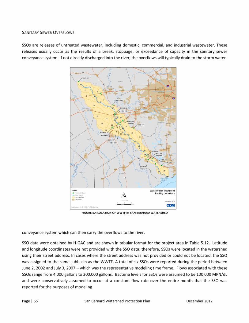
Page | 55 San Bernard Watershed Protection Plan December 2012
SANITARY SEWER OVERFLOWS
SSOs are releases of untreated wastewater, including domestic, commercial, and industrial wastewater. These
releases usually occur as the results of a break, stoppage, or exceedance of capacity in the sanitary sewer
conveyance system. If not directly discharged into the river, the overflows will typically drain to the storm water
FIGURE 5.4 LOCATION OF WWTF IN SAN BERNARD WATERSHED
conveyance system which can then carry the overflows to the river.
SSO data were obtained by H-GAC and are shown in tabular format for the project area in Table 5.12. Latitude
and longitude coordinates were not provided with the SSO data; therefore, SSOs were located in the watershed
using their street address. In cases where the street address was not provided or could not be located, the SSO
was assigned to the same subbasin as the WWTF. A total of six SSOs were reported during the period between
June 2, 2002 and July 3, 2007 – which was the representative modeling time frame. Flows associated with these
SSOs range from 4,000 gallons to 200,000 gallons. Bacteria levels for SSOs were assumed to be 100,000 MPN/dL
and were conservatively assumed to occur at a constant flow rate over the entire month that the SSO was
reported for the purposes of modeling.
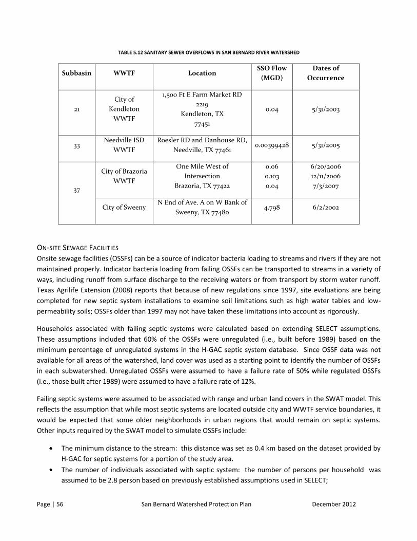
Page | 56 San Bernard Watershed Protection Plan December 2012
TABLE 5.12 SANITARY SEWER OVERFLOWS IN SAN BERNARD RIVER WATERSHED
Subbasin WWTF Location SSO Flow
(MGD)
Dates of
Occurrence
21
City of
Kendleton
WWTF
1,500 Ft E Farm Market RD
2219
Kendleton, TX
77451
0.04 5/31/2003
33 Needville ISD
WWTF
Roesler RD and Danhouse RD,
Needville, TX 77461 0.00399428 5/31/2005
37
City of Brazoria
WWTF
One Mile West of
Intersection
Brazoria, TX 77422
0.06
0.103
0.04
6/20/2006
12/11/2006
7/3/2007
City of Sweeny N End of Ave. A on W Bank of
Sweeny, TX 77480 4.798 6/2/2002
ON-SITE SEWAGE FACILITIES
Onsite sewage facilities (OSSFs) can be a source of indicator bacteria loading to streams and rivers if they are not
maintained properly. Indicator bacteria loading from failing OSSFs can be transported to streams in a variety of
ways, including runoff from surface discharge to the receiving waters or from transport by storm water runoff.
Texas Agrilife Extension (2008) reports that because of new regulations since 1997, site evaluations are being
completed for new septic system installations to examine soil limitations such as high water tables and low-
permeability soils; OSSFs older than 1997 may not have taken these limitations into account as rigorously.
Households associated with failing septic systems were calculated based on extending SELECT assumptions.
These assumptions included that 60% of the OSSFs were unregulated (i.e., built before 1989) based on the
minimum percentage of unregulated systems in the H-GAC septic system database. Since OSSF data was not
available for all areas of the watershed, land cover was used as a starting point to identify the number of OSSFs
in each subwatershed. Unregulated OSSFs were assumed to have a failure rate of 50% while regulated OSSFs
(i.e., those built after 1989) were assumed to have a failure rate of 12%.
Failing septic systems were assumed to be associated with range and urban land covers in the SWAT model. This
reflects the assumption that while most septic systems are located outside city and WWTF service boundaries, it
would be expected that some older neighborhoods in urban regions that would remain on septic systems.
Other inputs required by the SWAT model to simulate OSSFs include:
The minimum distance to the stream: this distance was set as 0.4 km based on the dataset provided by
H-GAC for septic systems for a portion of the study area.
The number of individuals associated with septic system: the number of persons per household was
assumed to be 2.8 person based on previously established assumptions used in SELECT;

Page | 57 San Bernard Watershed Protection Plan December 2012
The amount of discharge associated with septic systems: based on previous SELECT assumptions, a
discharge of 70 gallons/person/day was used in SWAT.
The concentration of bacteria associated with OSSF discharge: Bacteria concentrations associated with
failing systems was assumed to be 500,000 MPN/dL.
Based on the assumptions described above, a total of 6,817 failing OSSFs were simulated in the SWAT model
within the San Bernard River Watershed. Failing OSSF density throughout the watershed is presented in Table
5.13 and a plot of the septic system densities by subbasin is shown in Figure 5.5. Table 10.2 shows the number
of potentially failing septic systems in the San Bernard Watershed by subbasin and the number of systems that
would need to be repaired to meet water quality standards.
TABLE 5.13 FAILING ONSITE SEWAGE FACILITIES IN SAN BERNARD RIVER WATERSHED
Subbasin Septic Density
(km2)
Assumed distance from the Stream
(km)
1 5.48 0.422
2 4.89 0.422
3 12.40 0.422
4 13.80 0.422
5 9.33 0.422
6 6.16 0.422
7 7.78 0.422
8 10.28 0.422
9 11.65 0.422
10 20.05 0.422
11 17.75 0.422
12 7.73 0.422
13 9.53 0.422
14 15.69 0.422
15 16.17 0.422
16 21.41 0.422
17 25.80 0.422

Page | 58 San Bernard Watershed Protection Plan December 2012
Subbasin Septic Density
(km2)
Assumed distance from the Stream
(km)
18 27.63 0.422
19 16.40 0.422
20 36.91 0.422
21 21.88 0.422
22 18.89 0.422
23 32.28 0.422
24 17.82 0.422
25 17.91 0.422
26 60.93 0.422
27 33.69 0.422
28 19.10 0.422
29 42.52 0.422
30 23.26 0.422
31 33.20 0.422
32 24.24 0.422
33 21.21 0.422
34 10.02 0.422
35 37.38 0.422
36 129.31 0.422
37 77.54 0.422
38 61.05 0.422
39 51.49 0.422
40 7.70 0.422

Page | 59 San Bernard Watershed Protection Plan December 2012
FIGURE 5.5 SEPTIC DENSITY IN SAN BERNARD WATERSHED
AGRICULTURE
Although no CAFOs exist within the San Bernard River Watershed, there are a significant number of livestock
farms in the watershed that can serve as a potential source of bacteria.
Livestock estimates were obtained from the National Agriculture Statistical Service Census, which provides
livestock estimates by county. Shown in Table 5.14 are estimates for 2007 for cattle, sheep and goats and
horses. For input into SWAT, livestock estimates were aggregated based on Animal Equivalent Units (as shown
in Table 5.14) and were applied to range areas and 90% of pasture areas (as shown in Table 5.15). The concept
of animal equivalent units is well known in agriculture.

Page | 60 San Bernard Watershed Protection Plan December 2012
TABLE 5.14 COUNTY ANIMAL CENSUS RESULTS AND ANIMAL EQUIVALENT UNITS
Animal Animal Equivalent Units County Population
Cattle 1.000 Austin 70,184
Brazoria 78,560
Colorado 98,283
Fort Bend 46,206
Wharton 76780
Sheep & Goats 0.175 Austin 1,930
Brazoria 5,481
Colorado 1,036
Fort Bend 1,258
Wharton 3,591
Horses 1.250 Austin 3,491
Brazoria 5,367
Colorado 1,897
Fort Bend 3,105
Wharton 1,942
Bacteria loading associated with livestock is simulated using the grazing management option in SWAT. Livestock
grazing was associated with hay and range lands (both herbaceous and brush). For each subwatershed and
hydrologic response code, the model requires information on the number of grazing days, the amount of
manure produced by the livestock and the amount of biomass eaten. The number of grazing days in the
watershed was assumed to be 365 days per year and the dry weight of biomass consumed was 18 dry kg/day
per animal (Coffey, 2010). Presented in Tables 5.15 and 5.16 are assumptions used for livestock manure
characteristics to specify required SWAT parameters.
WILDLIFE AND UNMANAGED ANIMAL CONTRIBUTION
Deer, feral hogs, and geese are typical in this watershed. A typical value for deer densities in the area, based on
the Deer Density I-Map provided by the Quality Deer Management Association estimated on average 30 head
per acre, with a range of between 15 and 45 head per acre. Deer were assumed to be prevalent in 90% of

Page | 61 San Bernard Watershed Protection Plan December 2012
pasture areas plus forested areas (both mixed deciduous and evergreen) based on previous SELECT modeling
assumptions.
Feral hogs were assumed to have a density of five hogs per square kilometer based on values applied in the
SELECT modeling. SELECT data also provided a density of three hogs per square kilometer for bare land area,
however that land cover was not included in the SWAT model due to bare land only comprising 0.1% of the total
land area of the watershed and not meeting the threshold to be included as a land cover for SWAT analysis.
Three types of geese were evaluated: light goose species, Greater White-Fronted Goose, and Canada Goose).
The three geese species were aggregated into a single wildlife species, primarily made up from the light goose
species. Geese densities were based on data provided by H-GAC, and as per guidance with the data, were
assumed to be in agricultural and coastal marsh/prairie areas.
Bacteria loading associated with wildlife is simulated using the continuous fertilizer option in SWAT. For each
subwatershed and hydrologic response code, the model requires information the number of days fertilizer is
applied, the frequency of fertilizer application, and on the amount of manure produced by the wildlife. The
number of days fertilizer is applied was assumed to be 365 days per year and frequency of fertilizer application
was once per day (the most frequent option). For the manure production input, the total production for all
wildlife in a subbasin was summed and input as a single value and bacteria concentrations are adjusted to reflect
the variation expected in bacteria concentrations in manure. Presented in Tables 5.15 and 5.16 are assumptions
used for wildlife manure characteristics to specify required SWAT parameters.
DOMESTIC PETS
Domesticated animals, such as dogs and cats, can be a source of bacteria to San Bernard River Watershed via
nonpoint source runoff from high and low density residential land covers. The American Veterinary Medical
Association (2007) reports that 37.2% of all households own a dog and 32.4% of the households own cats. Using
U.S. Census data at the tract level (U.S. Census Bureau, 2008), census population estimates were used to
determine the approximate number of domestic pets within the project area; an average of 0.8 pets per
household was used for this study based on the inputs for the SELECT modeling. Domestic pets were assumed
to be distributed to the same land covers as used for septic systems, urban and rural areas (i.e., range land
covers).
TABLE 5.15 MANURE PHYSICAL CHARACTERISTICS FOR ANIMALS
Animal Production
(kg/day/animal)
Moisture Production (dry
kg/day/animal)
Source(s)
Livestock (used values for
beef cattle) 36 - 58 85% 5.4 - 8.7
1, 3, 4
Geese (used values for - - 0.03 – 0.18 2, 3
Deer 4.5 75%a 1.1 3

Page | 62 San Bernard Watershed Protection Plan December 2012
Feral Hogs (used values for
swine) 84 86% b
12.6
1
Dog 0.45 75% a
0.11 5
Source 1: ASAE Manure Production Standards (2005)
Source 2: Little Sac TMDL, http://dnr.mo.gov/env/wpp/tmdl/1381-l-sac-r-tmdl.pdf
Source 3: Parajuli, 200y. SWAT Bacteria Sub-Model Evaluation And Application
Source 4: Coffey et al., 2010. Development of Pathogen Transport model for Irish Catchments with SWAT
Source 5: Fecal coliform TMDL for the Ortega River, FDEP,
http://www.dep.state.fl.us/water/tmdl/docs/tmdls/final/gp2/fecaltmdl_ortegarive.pdf
Notes: a assume equivalent to sheet;
b assume equivalent to livestock
TABLE 5.16 MANURE BACTERIA CHARACTERISTICS FOR ANIMALS
Animal Fecal coliform concentration
(cfu/day-animal)d
Source
Livestock 4.29 x 10⁹ - 3.3 x 10
10 1, 2
Geese 8.00 x 10⁸
1
Deer 2.78 x 10⁸ - 3.6 x 10
8 1, 2
Feral hogs 7.06 109 - 3.3 x 10
10 2, 3
Dog 4.50 x 10⁸
- 3.97 x 10⁹ 1, 2
Source 1: Bacteria Source Loading Calculator, Virginia Tech (2006) http://www.tmdl.bse.vt.edu/outreach/C85/
Source 2: SELECT modeling
Source 3: Assumed same as livestock

Page | 63 San Bernard Watershed Protection Plan December 2012
FIGURE 5.6 TOTAL E. COLI LOADINGS BY SUBWATERSHED AND PERCENT CONTRIBUTION BY SOURCE
REFERENCES
USEPA. 1999. Draft guidance for water quality based decisions: The TMDL process, 3‐1 ‐ 3‐18. 2nd
ed. EPA841‐D‐99‐001. Washington, D.C.: U.S. Environmental Protection Agency, Office of Water.
USEPA. 2001. Protocol for developing pathogen TMDLs: Source assessment, 5‐1 ‐ 5‐18. 1st ed.
EPA841‐R00‐002. Washington,D.C.: U.S. Environmental Protection Agency, Office of Water.
Teague, A. E., 2007. Spatially Explicit Load Enrichment Calculation Tool and Cluster Analysis
for Identification of E. coli Sources in Plum Creek Watershed, Texas. Unpublished MS
thesis. Texas A&M University, Department of Biological and Agricultural Engineering,
College Station, Texas.
Page | 64 San Bernard Watershed Protection Plan December 2012
Reed, Stowe & Yanke, LLC. 2001 Study to Determine the Magnitude of, and Reasons for, Chronically
Malfunctioning On-Site Sewage Facility Systems in Texas. September 2001.
Doyle, M., and M. Erikson. 2006. Closing the door on the fecal coliform assay. Microbe 1(4): 162‐163.
USCB. 2000. Census 2000 TIGER/Line files. Washington, D.C.:
U.S. Census Bureau. Available at: www.census.gov/geo/www/tiger/index.html. Accessed 14 December
2006.
Exum, L. R., Bird, S. L., Harrison, J., and Perkins, C. A. (2005). “Estimating and Projecting Impervious
Cover in the Southeastern United States.” EPA,, Washington D.C.
Zeckoski, R., B. Benham, S. Shah, M. Wolfe, K. Brannan, M. Al‐Smadi, T. Dillaha, S. Mostaghimi, and D.
Heatwole. 2005.BLSC: A tool for bacteria source characterization for watershed management. Applied
Eng. in Agric. 21(5): 879‐889.
Hellgren, E. 1997. Biology of feral hogs (Sus scrofa) in Texas. In Proc. Feral Swine Symposium, 50‐58.
College Station, Tex.:Texas Cooperative Extension Service.

Page | 65 San Bernard Watershed Protection Plan December 2012
6 – ESTIMATED LOAD REDUCTIONS (ELEMENT B) Below is a table showing the percent load reductions needed by source as determined in the SWAT modeling.
Overall a 70% reduction in the bacteria geomean is required in the watershed. Load reductions by
subwatershed can be found in the appendices along with a box plot of source loading. Percent load reductions
were determined by :(Baseline E. coli concentration – E. coli concentration when source removed) / Baseline E.
coli concentration.
TABLE 6.1 – PERCENT REDUCTION FROM E. COLI GEOMEAN TO MEET WATER QUALITY STANDARD
Source Average Load
Contribution
(cfu/day)
Relative
Percentage
Reduction
Required
Wildlife 5.79E+11 40%
Septics 4.83E+11 33%
Livestock 2.55E+11 18%
Point Source 1.43E+11 10%
SWAT MODEL PERFORMANCE
As with the hydrology, a calibration period of up to two years was selected as per the project Quality Assurance
Project Plan (QAPP). The selected period was the same for the hydrology calibration as for the bacteria
calibration. Model performance for bacteria was evaluated on the basis of several criteria including:
Comparisons of observed grab samples to daily model bacteria concentrations; and
Long-term geometric mean comparisons.
Model performance was also evaluated using time series and overall geometric mean comparisons to observed
data collected by TCEQ and/or H-GAC at several monitoring stations. There are data starting in 2010 at recently
added monitoring stations, specifically 20722 and 20723. Because the model simulation period did not extend
beyond 2009, these stations could not be used specifically for calibration. However, the data at these stations
were used to give a general understanding of typical bacteria concentrations at those two locations and
parameters in the model were adjusted to match the general trends observed at those stations.
Results from the modeling are presented in Table 12 for the calibration period and Table 13 for the validation
period. The results presented in these tables are for paired results, meaning that the simulated bacteria
concentration was matched with an observed data point and the geometric means were calculated using those
data. As can be seen from the table, there are some stations where the model matched very well, such as
Station 16373. Other stations, such as 12147, did not match as well on a paired basis. This is not unexpected
for bacteria simulations.

Page | 66 San Bernard Watershed Protection Plan December 2012
TABLE 6.2 – BACTERIA SIMULATION PERFORMANCE – CALIBRATION PERIOD (CONCENTRATIONS IN CFU/DL)
Station
Number of
Samples
Observed
Geometric Mean
Modeled
Geometric Mean Error1
16373 16 303.3 301.9 2%
17420 9 317.0 91.6 -74%
12147 18 412.5 753.3 225%
15272 12 428.3 229.2 -48%
1. Error is calculated as observed concentration minus the modeled value divided by the observed
value.
TABLE 6.3 – BACTERIA SIMULATION PERFORMANCE – PAIRED DATASET FOR VALIDATION PERIOD (CONCENTRATIONS IN CFU/DL)
Station Number of
Samples
Observed
Geometric Mean
Modeled
Geometric Mean Error
1
16370 16 78.1 366.9 370%
16373 9 295 301 2%
12147 18 282.4 918.1 225%
1. Error is calculated as observed concentration minus the modeled value divided by the
observed value.
TIDAL PRISM MODEL PERFORMANCE
The model performance for the tidal prism for bacteria was evaluated by comparing the observed enterococci to
modeled enterococci at all available stations along the main stem of the stream on an overall geometric mean
basis as well as by comparing individual grab samples to simulated values.
A longitudinal plot of the modeled and observed geometric mean concentrations for the calibration period is
presented in Figure 6.1 for the calibration period and Figure 6.2 for the validation period. The maximum and
minimum concentrations presented in the longitudinal plot are the maximum/minimum geometric means for
each year of the calibration time period. The validation time period was not long enough to calculate geometric
means for more than one year; therefore, only the geometric mean was plotted on the graph. Time series plots
for each of the stations are also presented in Figure 6.2 for the calibration period and Figure 6.3 for the
validation period. Segment 2 exhibits small changes in concentration that reflect the tidal fluctuation in the San
Bernard River. The peaks observed in the data are related to rainfall events which cause runoff from the

Page | 67 San Bernard Watershed Protection Plan December 2012
watershed to reach the tidal segment of the San Bernard River, carrying with it elevated concentrations of
bacteria. While it can be seen that the model does overestimate in some segments and underestimates in
others, overall it captures the bacterial levels in San Bernard River.
FIGURE 6.1 – BACTERIA LONGITUDINAL PLOT – CALIBRATION (JANUARY 1, 2007 – DECEMBER 31, 2008)
FIGURE 6.2 – BACTERIA LONGITUDINAL PLOT – VALIDATION (JANUARY 1, 2009 THROUGH SEPTEMBER 30, 2009)
1
10
100
1000
10000
0510152025303540455055
Ente
roco
cci (
MP
N/d
L)
Distance from Intercoastal Water Way (Km)
Minimum
Geomean
Maximum
Observed - Cal period
Enterococci Standard
1
10
100
1000
10000
0510152025303540455055
Ente
roco
cci (
MP
N/d
L)
Distance from Intercoastal Water Way (Km)
Geomean
Observed - Val period
Enterococci Standard

Page | 68 San Bernard Watershed Protection Plan December 2012
FIGURE 6.3 –TIME SERIES PLOTS – CALIBRATION PERIOD
BACTERIA SOURCE ANALYSIS
There are several potential sources of bacteria in the San Bernard River Watershed. These include permitted
sources, such as wastewater treatment facilities that do not completely disinfect their effluent and sanitary
sewer overflows. Other sources, such as livestock, wildlife, domestic pets, and failing on-site sewage facilities
(septic systems) are not permitted but may also contribute to bacteria loading in the San Bernard River.
To explore the impact of each of these sources, several scenarios were run using SWAT with each source
eliminated. The change in the in-stream concentrations of bacteria indicate how significant an impact each of
the sources have on the San Bernard River. Since the majority of these changes occur in the watershed, the
SWAT model was the only tool used to evaluate the sources in the River. The results of the analysis are
presented in Figure 6.4.
The figure demonstrates that all bacteria sources in the watershed play a role in maintaining the bacteria levels
in the River. This is an important finding as it suggests that improving water quality in the River can be achieved
in multiple ways. It is important to note that these scenarios are used as a tool to understand the watershed; it
is not expected that any of the source elimination scenarios would be physically implemented in the watershed.
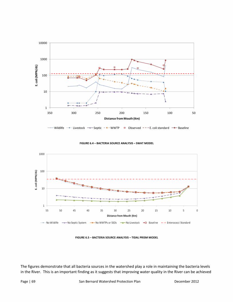
Page | 69 San Bernard Watershed Protection Plan December 2012
FIGURE 6.4 – BACTERIA SOURCE ANALYSIS – SWAT MODEL
FIGURE 6.5 – BACTERIA SOURCE ANALYSIS – TIDAL PRISM MODEL
The figures demonstrate that all bacteria sources in the watershed play a role in maintaining the bacteria levels
in the River. This is an important finding as it suggests that improving water quality in the River can be achieved
1
10
100
1000
10000
50100150200250300350
E. c
oli
(MP
N/d
L)
Distance from Mouth (Km)
Wildlife Livestock Septic WWTP Observed E. coli standard Baseline

Page | 70 San Bernard Watershed Protection Plan December 2012
in multiple ways. It is important to note that these scenarios are used as a tool to understand the watershed; it
is not expected that any of the source elimination scenarios would be physically implemented in the watershed.
A summary table of the reductions based on each source is presented in Table 6.4 for the SWAT model and
Table 6.5 for the Tidal Prism model.
TABLE 6.4. SUMMARY OF E. COLI CONCENTRATIONS AND PERCENT REDUCTION FROM BASELINE CONDITION – SWAT MODEL
Subbasin River Km
Baseline No WWTFs or SSOs No Wildlife No Septic Systems No Livestock
E. c
oli
(MP
N/d
L)
E. c
oli
(MP
N/d
L)
Pe
rce
nt
Re
du
ctio
n
E. c
oli
(MP
N/d
L)
Pe
rce
nt
Re
du
ctio
n
E. c
oli
(MP
N/d
L)
Pe
rce
nt
Re
du
ctio
n
E. c
oli
(MP
N/d
L)
Pe
rce
nt
Re
du
ctio
n
1 312.09 87.8 87.2 -1% 20.7 -76% 1.4 -98% 2.0 -98%
7 293.11 90.4 90.1 0% 22.5 -75% 1.3 -99% 1.9 -98%
8 289.04 93.6 93.4 0% 24.7 -74% 1.3 -99% 1.9 -98%
10 273.77 62.1 62.0 0% 16.8 -73% 1.4 -98% 2.0 -97%
11 254.09 122.9 117.6 -4% 40.0 -67% 2.0 -98% 9.8 -92%
13 246.50 332.2 318.8 -4% 26.9 -92% 9.6 -97% 110.7 -67%
16 237.75 282.3 272.6 -3% 23.0 -92% 9.3 -97% 96.3 -66%
17 215.14 279.0 273.1 -2% 15.5 -94% 9.6 -97% 115.3 -59%
21 200.00 274.8 256.6 -7% 14.7 -95% 9.4 -97% 122.9 -55%
23 187.65 272.8 268.6 -2% 26.8 -90% 8.5 -97% 90.8 -67%
26 179.27 1085.0 1079.6 0% 305.9 -72% 8.0 -99% 64.7 -94%
28 173.90 956.8 953.8 0% 268.7 -72% 7.6 -99% 58.1 -94%
30 166.97 818.5 817.1 0% 233.3 -71% 7.4 -99% 52.1 -94%
31 139.05 554.9 554.7 0% 159.3 -71% 6.9 -99% 41.6 -93%
35 112.85 291.8 273.9 -6% 82.8 -72% 7.4 -97% 37.5 -87%
34 108.76 1246.9 1246.9 0% 412.1 -67% 2.4 -100% 10.5 -99%

Page | 71 San Bernard Watershed Protection Plan December 2012
TABLE 6.5. SUMMARY OF ENTEROCOCCI CONCENTRATIONS AND PERCENT REDUCTION FROM BASELINE CONDITION – TIDAL PRISM MODEL
River KM/Segment
Baseline No WWTFs or SSOs No Wildlife No Septic Systems No Livestock
Ente
roco
c
ci
(MP
N/d
L)
Ente
roco
c
ci
(MP
N/d
L)
Pe
rce
nt
Re
du
ctio
n
Ente
roco
c
ci
(MP
N/d
L)
Pe
rce
nt
Re
du
ctio
n
Ente
roco
c
ci
(MP
N/d
L)
Pe
rce
nt
Re
du
ctio
n
Ente
roco
c
ci
(MP
N/d
L)
Pe
rce
nt
Re
du
ctio
n
32.00 37.8 38.4 2% 35.1 -7% 4.0 -89% 2.2 -94%
30.00 27.7 27.8 0% 24.6 -11% 3.5 -87% 2.2 -92%
28.00 20.8 20.6 -1% 17.9 -14% 3.2 -85% 2.1 -90%
26.00 15.3 15.6 2% 13.5 -12% 2.9 -81% 2.0 -87%
24.00 12.2 12.5 2% 10.7 -12% 2.7 -78% 1.9 -84%
22.00 10.0 10.2 2% 8.8 -11% 2.6 -74% 1.9 -81%
20.00 8.4 8.7 3% 7.6 -10% 2.5 -71% 1.8 -79%
18.00 7.3 7.5 3% 6.7 -8% 2.4 -67% 1.8 -75%
16.00 6.5 6.7 3% 6.1 -6% 2.4 -63% 1.8 -72%
14.00 6.0 6.2 3% 5.8 -4% 2.5 -58% 1.9 -69%
12.00 5.6 5.8 3% 5.6 -1% 2.7 -52% 2.0 -64%
10.00 5.5 5.6 3% 5.5 1% 3.0 -44% 2.3 -59%
8.00 5.6 5.8 3% 5.8 3% 3.6 -36% 2.6 -53%
6.00 6.0 6.2 2% 6.2 4% 4.5 -26% 3.2 -48%
4.00 6.5 6.6 2% 6.7 3% 5.5 -15% 3.8 -41%
2.00 13.0 13.0 0% 13.0 0% 13.0 0% 13.0 0%
Key findings are as follows:
Wastewater treatment facilites: It was assumed that the discharge associated with WWTFs would be
126 MPN/dL for the baseline condition, which is the current water quality standard for E. coli. SSOs were
assigned a concentration of 500,000 MPN/dL which is consistent with dilute sewage concentrations.
The source elimination scenario eliminated all bacteria in the effluent discharge. In practice, the
concentrations associated with the discharges will vary based upon a wide range of factors such as plant
condition, plant maintenance, and occurrence of rainfall. However, it is clear from the modeling that

Page | 72 San Bernard Watershed Protection Plan December 2012
wastewater treatment plants do play a small role in maintaining the elevated bacteria concentrations in
the current baseline model.
Septic systems: Septic systems proved to be a significant factor in the elevated concentrations observed
in the San Bernard River. This scenario assumed that all malfunctioning septic systems were fixed and
therefore no discharge of bacteria occurred. The difference in bacteria concentrations with and without
failing septic systems is striking and suggests that there is a significant impact from the systems on the
San Bernard River.
Livestock: The modeling suggests that bacteria runoff from livestock manure is another key factor that
maintains the elevated bacteria in the San Bernard River. It is clear that livestock are another key factor
in maintaining the bacteria concentrations in the San Bernard River. Livestock have more impact on the
upper reaches of the watershed than other locations. It is important to note that the livestock (and
wildlife) estimates for some subbasins were calibrated higher than what would be predicted based on
the animal census data to match the in-stream bacteria levels.
Wildlife and domesticated animals: Wildlife and domesticated animal loading in the watershed is
another key source of bacteria in the region. Eliminating their contributions does not permit the San
Bernard to meet water quality standards.
BMP SCENARIO EVALUATION
Modeling determined that there are a number of different causes and sources of pollution in the San Bernard
Watershed, and that there are a number of BMPs that will work to reduce pollution levels in the watershed.
Vegetative filter strips and grassed waterways were both evaluated by the SWAT model for their effectiveness in
pollution removal for the four categories of pollution that were examined. There are also a number of other
BMPs that were not modeled specifically for the San Bernard watershed, but that have been tested in other
watersheds for effectiveness. These BMPs and their estimated load reductions are presented in the appendices
on pages 131 -132. Some BMPs are multi-purpose such as the vegetative filter strips and the grassed
waterways, and some are more source specific, such as fixing failing OSSFs. Water Quality Management Plans
are common throughout the watershed, and are specific to each property they protect.
After evaluating the impact of each bacteria source on the San Bernard River watershed, the next step was to
evaluate some specific BMPs that could be implemented in the watershed to improve water quality. The
following section outlines some potential BMP solutions.
BMP SCENARIO 1 - VEGETATIVE FILTER STRIPS
One type important management practice (BMP) for water pollution in agricultural areas is a vegetative filter
strip. Vegetative filter strips (VFSs) are also known as buffer strips, riparian zones, protection strips, and
streamside management zones. Filter strips are located adjacent to the stream to help protect water quality of
the stream or lake. These strips are used to minimize the effect of agricultural uses, grazing, and urban activity
around the watershed. Filter strips prevent bacteria, sediments, organics, nutrients, pesticides, and other
contaminant loadings from entering the streams and thus improving water quality.
SWAT models VFSs with two approaches: one that receives modest flow densities and one that receives
concentrated flows. The VFS channel geometry is defined as a trapezoidal with 8:1 side slope; the required

Page | 73 San Bernard Watershed Protection Plan December 2012
inputs for waterways are length, width, depth, and slope. In SWAT, the VFS functionality is simulated in two
sections; section 1 represents the bulk of the VFS area receiving the lower flows (i.e., is more diffuse) and
section 2 receives about 25% to 75% of the field runoff (the “headwaters” of the VFS that receives more
concentrated flow). One important point to note is that in VFSs, bacteria are assumed to be sorbed and
captured within the sediment and the soluble particles are captured on the runoff.
The VFSs were applied to agriculture (AGRR), hay (HAY), rangeland shrub (RNGB), and rangeland
grassland/herbaceous (RNGE) land covers. The filter strip was assumed to start at the beginning of the
simulation period. Several other key variables were specified for the VFS:
VFSRATIO is the ratio of field area to filter strip (ha²/ha²), ranges from 0 ha²/ha² to 300 ha²/ha² with 40
ha²/ha² to 60 ha²/ha² being common values, the values tested in the model were 45 ha²/ha² and 55
ha²/ha². These values indicate the density
The VFSCON variable refers to the fraction of the HRU that drains the most concentrated 10% of the
filters strip area, value of 50% was used per SWAT guidance.
VFSCH is the fraction of the flow of the most concentrated 10% of the filter strip; this value was set to
0% per SWAT guidance (Waidler et al, 2011).
Once all the variables were set, the edits were extended to all the subbasins containing the desired land covers
for all the different slopes.
The results of the analysis are presented in Figure 6.6. A summary of the concentrations in tabular form are
presented in Table 6.6 as well. As the figure demonstrates, vegetated filter strips implemented in the watershed
could have a very significant impact on the in-stream concentrations of bacteria. It is important to note that the
middle portion of the River is just above the water quality standard when the most significant improvements
are observed, indicating that some additional efforts will be required to reduce failing septic systems, improve
wastewater treatment or otherwise exclude cattle/wildlife from the streams.
1
10
100
1000
10000
50100150200250300350
E. c
oli
(MP
N/d
L)
Distance from Mouth (Km)
Ratio = 55 Ratio = 45 Observed E. coli standard Baseline

Page | 74 San Bernard Watershed Protection Plan December 2012
FIGURE 6.6 – VEGETATED FILTER STRIP RESULTS
TABLE 6.6. SUMMARY OF E. COLI CONCENTRATIONS AND PERCENT REDUCTION FROM BASELINE CONDITION – VEGETATED FILTER STRIP RESULTS
Subbasin River Km
Baseline
Ratio of filter are to filter strip
= 45
Ratio of filter are to filter
strip = 55
E. coli
(MPN/dL)
E. coli
(MPN/dL)
Percent
Reduction
E. coli
(MPN/dL)
Percent
Reduction
1 312.09 87.8 9.2 -90% 2.9 -97%
7 293.11 90.4 9.5 -89% 3.7 -96%
8 289.04 93.6 10.2 -89% 3.9 -96%
10 273.77 62.1 7.7 -88% 3.2 -95%
11 254.09 122.9 27.6 -78% 10.0 -92%
13 246.5 332.2 144.2 -57% 51.3 -85%
16 237.75 282.3 124.2 -56% 45.9 -84%
17 215.14 279.0 135.1 -52% 68.5 -75%
21 200 274.8 138.8 -49% 74.5 -73%
23 187.65 272.8 99.5 -64% 120.2 -56%
26 179.27 1085.0 162.1 -85% 860.9 -21%
28 173.9 956.8 147.1 -85% 762.6 -20%
30 166.97 818.5 125.4 -85% 652.3 -20%
31 139.05 554.9 90.2 -84% 443.0 -20%
35 112.85 291.8 62.9 -78% 237.4 -19%
34 108.76 1246.9 58.2 -95% 455.9 -63%
The model does not specify a specific sorption rate, but does have several parameters that specify the
relationship between bacteria and soil: Bacteria soil partitioning coefficient (BACTKDQ) is the ratio of the
bacteria concentration in the surface 10 mm of soil water to the concentration of bacteria in surface
runoff. Higher values result in lower concentrations of bacteria in the surface runoff. The value for the San
Bernard watershed was set to 175; this default value has been found to be appropriate in several other SWAT
Page | 75 San Bernard Watershed Protection Plan December 2012
modeling applications. Bacteria percolation coefficient (BACTMIX) is the ratio of bacteria concentrations in the
top 10 mm of soil to the concentration of bacteria in the percolate. The model default value is 10.0 and the
value can range from 7.0 to 20.0. The value for the San Bernard watershed was set to 10.0 based on other
studies that have applied the default value.
It is interesting that the more concentrated filter strips (those with a ratio of filter area to filter strip of 45
ha²/ha²) result in lower concentrations near the mouth of watershed when compared with the less
concentrated filter strips (those with ratio of filter area to filter strip of 55 ha²/ha²). This may be related to the
flatter land near the mouth of the watershed which may not respond as well to the filter strips. In the upper
watershed, a less concentrated filter strip could potentially result in a longer flow path along the filter strip and
thus remove additional bacteria from stormwater runoff.
BMP SCENARIO 2 - GRASSED WATER WAYS
Grassed waterways are another type of BMP for bacterial water pollution. Grassed waterways are strips of grass
seeded in areas where water concentrates or flows off a field. These patches are planted with strong roots grass
to carry water across a land. These waterways provide benefits such as reducing the flow velocity, trap
sediment and bacteria, absorb chemicals and nutrients from the runoff water, and provide enhancements to
wildlife.
SWAT models grassed waterways as a trapezoidal channel. SWAT simulates the channel as broad and shallow
with side slopes of 8:1. The reduction of sediments, bacteria and nutrients are calculated in a similar fashion to
the way the model simulates sediment and organic nutrient loss for subbasin tributary channels. The main
inputs are width and length. Grassed waterway is simulated on an HRU basis, meaning that they can be varied
by land cover.
The grassed waterways were applied to the same land covers as VFSs, agriculture (AGRR), hay (HAY), rangeland
shrub (RNGB), and rangeland grassland/herbaceous (RNGE) land covers. The grassed waterways were assumed
to be in place at the beginning of the simulation period. The following key variables were used to simulate
grassed waterways
GWATN: SWAT requires a Manning’s N used for overland flow, under the variable GWATN. The
Manning’s n selected was 0.35 to represent the overland flow.
GWATSPCON is a linear parameter for the sediments in the waterways, the default value of 0.005 was
used for the variable.
GWATL is the length of the grassed waterway is entered under the GWATL variable. The length was
varied between 5, 25 and 50 km in length. This default is the length of a single side of a squared HRU.
GWATD is the depth of the channel from top of the bank to the bottom in meters. If a depth is not
selected the program sets the depth as 3/64 of GWATW. For the 5 and 25 m long channels, a value of 1
m was used. For the channel with 50 m in length, a value of 2 m was used.
GWATW is the average width in meters of the grassed waterway. For the evaluation of the alternative
widths of 100 meters were used.

Page | 76 San Bernard Watershed Protection Plan December 2012
GWATS is the average slope of the channel in meters. The default value of 0.005 was used for the slope.
If the slope is not entered SWAT calculates the slope as 75% of the HRU slope.
Results from the analyses are presented in Figure 6.7. A tabular summary of the results are presented in
Table 6.7. As shown, there is some reduction in bacteria concentrations when the BMPs are implemented.
The results suggest that implementing grassed waterways in the San Bernard River watershed will result in
an improvement in water quality; however, the impact of these BMPs will not be as significant as the
vegetated filter strips.
FIGURE 6.7 – GRASSED WATERWAYS
TABLE 6.7 - SUMMARY OF E. COLI CONCENTRATIONS AND PERCENT REDUCTION FROM BASELINE CONDITION – GRASSED WATERWAY RESULTS
Subbasin
River
Km
Baseline
Waterway length = 5
m
Waterway length = 25
m
Waterway length = 50
m
E. coli
(MPN/dL)
E. coli
(MPN/dL)
Percent
Reduction
E. coli
(MPN/dL)
Percent
Reduction
E. coli
(MPN/dL)
Percent
Reduction
1 312.09 87.8 78.4 -11% 57.8 -34% 57.8 -34%
7 293.11 90.4 80.7 -11% 59.4 -34% 59.4 -34%
8 289.04 93.6 83.2 -11% 61.1 -35% 61.1 -35%
10 273.77 62.1 55.6 -11% 41.1 -34% 41.1 -34%
11 254.09 122.9 116.7 -5% 91.4 -26% 91.4 -26%
13 246.5 332.2 329.9 -1% 287.9 -13% 287.9 -13%
16 237.75 282.3 280.2 -1% 244.9 -13% 244.9 -13%
17 215.14 279.0 277.0 -1% 245.6 -12% 245.6 -12%
1
10
100
1000
10000
50100150200250300350
E. c
oli
(MP
N/d
L)
Distance from Mouth (Km)Length = 25 m Length = 50 m Length = 5 m Observed E. coli standard Baseline

Page | 77 San Bernard Watershed Protection Plan December 2012
21 200 274.8 273.0 -1% 243.6 -11% 243.6 -11%
23 187.65 272.8 258.5 -5% 222.5 -18% 222.5 -18%
26 179.27 1085.0 991.1 -9% 774.5 -29% 774.5 -29%
28 173.9 956.8 871.5 -9% 679.6 -29% 679.6 -29%
30 166.97 818.5 742.2 -9% 577.6 -29% 577.6 -29%
31 139.05 554.9 504.2 -9% 393.2 -29% 393.2 -29%
35 112.85 291.8 268.4 -8% 213.6 -27% 213.6 -27%
34 108.76 1246.9 1037.0 -17% 733.7 -41% 733.7 -41%
BMP SCENARIO 3 – OSSF REPAIR AND REPLACEMENT
On-site septic systems are a significant factor in the elevated bacteria concentrations observed in the San
Bernard Watershed. This BMP focused on the repair and replacement of OSSFs in two specific subbasins: 36 and
25. The model was fairly insensitive to the OSSF densities within the subbasins, so the analysis was focused on
assuming that all OSSFs in a subbasin would be repaired or replaced. The results show an immediate decrease
in bacteria downstream of these two subbasins, as shown in the figures below.
TABLE 6.8 - SUMMARY OF E. COLI CONCENTRATIONS AND PERCENT REDUCTION FROM BASELINE CONDITION – OSSF REPAIR AND REPLACEMENT
Subbasin
River
Km
Baseline
Subbasin 36 OSSF
Repair/Replacement
Peach Creek Watershed
Repair/Replacement
E. coli
(MPN/dL)
E. coli
(MPN/dL)
Percent
Reduction
E. coli
(MPN/dL)
Percent
Reduction
1 312.09 87.8 87.8 0% 87.8 0%
7 293.11 90.4 90.4 0% 90.4 0%
8 289.04 93.6 93.6 0% 93.6 0%
10 273.77 62.1 62.1 0% 62.1 0%
11 254.09 122.9 122.9 0% 122.9 0%
13 246.5 332.2 332.3 0% 332.3 0%
16 237.75 282.3 282.3 0% 282.3 0%
17 215.14 279.0 279.0 0% 279.0 0%

Page | 78 San Bernard Watershed Protection Plan December 2012
21 200 274.8 274.8 0% 274.8 0%
23 187.65 272.8 272.8 0% 272.8 0%
26 179.27 1085.0 1085.0 0% 1085.0 0%
28 173.9 956.8 956.7 0% 636.9 -33%
30 166.97 818.5 818.5 0% 581.0 -29%
31 139.05 554.9 554.9 0% 428.7 -23%
35 112.85 291.8 291.8 0% 267.0 -8%
34 108.76 1246.9 1247.0 0% 1247.0 0%
FIGURE 6.8 – OSSF REPAIR AND REPLACEMENT

Page | 79 San Bernard Watershed Protection Plan December 2012
BMP SCENARIO 4 – PRESCRIBED GRAZING
Prescribed grazing is another BMP for bacterial water pollution. Prescribed grazing is the management of the
removal of vegetation by grazing animals with respect to plant production limits, sensitivities and management
goals. The rate of growth and physiological condition of the plants, duration and intensity of grazing, and
expected productivity of the forage species are other management objectives that are taken into account when
preparing a prescribed grazing program.
The focus of this BMP was on grazing analysis for pasture and range land covers, and included modification to
several parameters to simulate grazing. These parameters include: moisture, harvest efficiency, and soil loss.
Moisture values represent soil permeability, land cover, and antecedent moisture conditions. Higher moisture
values indicate improved crop management, but lower permeability coverage, while lower values indicate
higher permeability, but poorer crop management. For this BMP, the values were lowered to simulate
improved crop management. Harvest efficiency is defined as the fraction of biomass removed by harvesting
equipment. For the model the value was increased which equates to increase cuttings being left on the ground.
The sensitivity analysis performed showed that the bacteria levels in the San Bernard watershed were not
sensitive to changes in harvest efficiency. Soil loss is the ratio of the erosion that would occur when a crop is
grown using a specific management practice as compared to leaving the continuously tilled fallow state without
vegetation. This value was already quite high for the San Bernard watershed, so it was not further adjusted.
With these adjustments made, it was found that there were only small reductions in bacteria levels compared
with the baseline conditions.
TABLE 6.9 - SUMMARY OF E. COLI CONCENTRATIONS AND PERCENT REDUCTION FROM BASELINE CONDITION – PRESCRIBED GRAZING
Subbasin
River
Km
Baseline
Prescribed Grazing
Scenario
E. coli
(MPN/dL)
E. coli
(MPN/dL)
Percent
Reduction
1 312.09 87.8 87.7 0%
7 293.11 90.4 91.1 -1%
8 289.04 93.6 92.6 -1%
10 273.77 62.1 61.5 -1%
11 254.09 122.9 118.9 -3%
13 246.5 332.2 322.1 -3%
16 237.75 282.3 273.8 -3%
17 215.14 279.0 272.7 -2%
21 200 274.8 267.6 -3%

Page | 80 San Bernard Watershed Protection Plan December 2012
23 187.65 272.8 264.4 -3%
26 179.27 1085.0 1060.9 -2%
28 173.9 956.8 939.5 -2%
30 166.97 818.5 802.7 -2%
31 139.05 554.9 549.4 -1%
35 112.85 291.8 289.3 -1%
34 108.76 1246.9 1093.5 -4%
FIGURE 6.9 – PRESCRIBED GRAZING
BMP SCENARIO 5 – FERAL HOG MANAGEMENT
Feral hogs and other wildlife are significant contributors of bacteria in the San Bernard watershed. Feral hog
densities in the watershed are estimated to be about 5 hogs per square kilometer, which results in about 10,000
hogs being found in the watershed. Feral hog management strategies were simulated at 30%, 50% and 75%
reductions in the watershed, although none showed a significant reduction in E. coli levels. While hog manure
production can make up a significant portion of the wildlife loading in some watersheds, wildlife manure

Page | 81 San Bernard Watershed Protection Plan December 2012
generally provides a much smaller contribution (usually 1% or less) than livestock manure loading. Therefore
the overall impact of feral hogs is quite small.
TABLE 6.10 - SUMMARY OF E. COLI CONCENTRATIONS AND PERCENT REDUCTION FROM BASELINE CONDITION – FERAL HOG MANAGEMENT
Subbasin
River
Km
Baseline
50% Reduction in Feral
Hogs
75% Reduction in Feral
Hogs
E. coli
(MPN/dL)
E. coli
(MPN/dL)
Percent
Reduction
E. coli
(MPN/dL)
Percent
Reduction
1 312.09 87.8 87.6 0% 87.5 0%
7 293.11 90.4 90.1 0% 89.8 -1%
8 289.04 93.6 93.2 0% 92.9 -1%
10 273.77 62.1 61.9 0% 61.7 -1%
11 254.09 122.9 122.6 0% 122.3 0%
13 246.5 332.2 332.0 0% 331.7 0%
16 237.75 282.3 282.1 0% 281.9 0%
17 215.14 279.0 287.8 0% 278.6 0%
21 200 274.8 274.6 0% 274.4 0%
23 187.65 272.8 272.7 0% 272.5 0%
26 179.27 1085.0 1082.4 0% 1081.1 0%
28 173.9 956.8 955.8 0% 953.3 0%
30 166.97 818.5 818.0 0% 816.5 0%
31 139.05 554.9 555.0 0% 554.6 0%
35 112.85 291.8 291.9 0% 291.8 0%
34 108.76 1246.9 1246.8 0% 1246.5 0%

Page | 82 San Bernard Watershed Protection Plan December 2012
FIGURE 6.10 - FERAL HOG MANAGEMENT
MODELING CONCLUSIONS
The vegetative filter strips, grassed waterways, and OSSF repairs and replacements are all effective in removing
pollutants from runoff before it enters waterway, however the vegetative filter strips and OSSF repairs and
replacements are the most effective. The location of the waterway and slope of the surrounding lands makes a
difference in the effectiveness of the BMP. The SWAT and Tidal Prism modeling demonstrates that there are a
number of ways in which to improve the water quality in the San Bernard watershed. Sources of the most
concern in the watershed include on-site sewage facilities, livestock, and wildlife. Best management practices
that help treat and prevent runoff from these sources from entering the waterways will be most useful in
lowering bacteria levels in the watershed. The modeling also demonstrated that significantly improving just one
or two of the sources would help improve the overall water quality in the watershed. The two sources that
would most significantly improve the water quality if they were at least partially eliminated would be OSSFs and
livestock. A few of the subwatersheds in particular that contribute greater inputs should be prioritized.
Page | 83 San Bernard Watershed Protection Plan December 2012
7 - MANAGEMENT MEASURES (ELEMENT C) A number of Best Management Practices (BMPs) were reviewed for the San Bernard Watershed Protection Plan.
These BMPs came from other Watershed Protection Plans, Water Quality Management Plans, and the TSSWCB’s
list of approved BMPs. A list of currently approved and implemented BMPs in the watersheds was also
examined. A comprehensive list of BMPs were presented to stakeholders to rank based on what they thought
was most needed in the watershed and what was likely to be implemented. The BMP activities that were ranked
the highest were: feral hog programs, repair and replacement of OSSFs, enforcement of illegal dumping and
disposal, and filter strips surrounding agricultural practices. The two BMPs that were modeled in the
watershed were vegetated filter strips and grasses waterways. The modeling determined that vegetated filter
strips would be very effective in removing pollutants before they reach waterways. This is a BMP that would be
effective across a number of different land cover types.
OSSFS
OSSFs have been identified as a major contributor to the loadings in the San Bernard watershed. When doing
SELECT and SWAT modeling it was assumed that 50% of the OSSFs installed prior to 1989 and 15% of the OSSFs
installed after 1989 were failing. A lot of the OSSFs in the watershed are older systems that may be
malfunctioning and need to be replaced. In many cases the system owners may not be aware that their OSSF is
malfunctioning. Malfunctioning systems are the result of over use, lack of maintenance, lack of education by
owners, and inappropriate soils for the type of system. Repair and replacement of OSSFs can have a 10% to 30%
reduction of released pollutants (SWERPC, 2008). OSSFs are prevalent throughout the watershed, but there are
fewer in proximity to the waterways in Colorado and Austin Counties. Brazoria County should be a priority for
repair and replacement of existing systems.
Updating design criteria and placement for new systems to ensure adequate space and soil types
Work with Authorized Agents to create a uniform reporting system, use of GPS in placement
Voluntary repair and replacement of older systems
Homeowner education workshops
WILDLIFE
Feral hogs have been identified as a major contributor to the bacteria loadings in the watershed. Feral hogs are
found throughout the watershed in urban and rural areas and are known to cause a lot of damage. There are
not a lot of BMPs that are highly effective in controlling the populations; however programs are being developed
in other watersheds that are helping build awareness and effectiveness. In addition to feral hogs there are also
a number of other wild animals in the watershed including raccoon, opossums, deer, and avian wildlife.
Programs to control feral hog populations should be a top priority for all of the jurisdictions of the watershed
since it is a statewide problem.
Feral Hog Programs with Texas AgriLife Extension Service and Texas Parks and Wildlife
Hog hunting and trapping programs to help reduce numbers
Page | 84 San Bernard Watershed Protection Plan December 2012
LIVESTOCK
Modeling has identified cattle as a source of concern in the San Bernard Watershed. A lot of pasture land
directly fronts the San Bernard River and its tributaries. Management measures for livestock can voluntarily be
implemented to keep cattle and their waste from entering the waterways. The TSSWCB also offers Water
Quality Management Plans to landowners in the watershed, and once approved landowners may be eligible for
funding to help implement the practices identified in the plan. Controlling animal waste entering streams can
have a 50% to 75% reduction of pollutants being released into streams (SWERPC, 2008). Water Quality
Management Plans that contain livestock BMPs are already occurring throughout the watershed.
Waste Management by creating temporary storage facilities for animal waste and contaminated water
Fencing to create a barrier to livestock and wildlife from entering streams and to assist in other
conservation efforts
Alternate Water Sources to provide water sources for livestock
Prescribed Grazing to manage vegetation with the use of grazing animals to reduce soil erosion
AGRICULTURE
Agricultural lands are not a major contributor to the total loadings in the San Bernard watershed; however
agricultural lands do make up the majority of the land cover in the watershed. The TSSWCB offers Water Quality
Management Plans to landowners in the watershed, and once approved, landowners may be eligible for funding
to help implement the practices identified in the plan. Conservation practices that help filter pollutants can
have up to a 50% reduction in the amount of pollutants released into waterways (SWERPC, 2008). Water
Quality Management Plans that contain agriculture BMPs are already occurring throughout the watershed.
Watershed Modeling demonstrated that contour buffer strips and filter strips were the most effective in
removing pollutants from runoff. These two BMPs should be given priority in WQMPs.
Nutrient Management to manage the amount, timing and placement of nutrients
Crop Residue Management to leave a protective layer of previous crop behind to help reduce erosion
Conservation Crop Rotation to grow various crops in rotation to reduce erosion and improve soil
Terracing to create ridges and channels to reduce slope length and reduce erosion and sediment runoff
Contour Buffer Strips to convey runoff without erosion and protect water quality
Filter Strips to reduce sediment, organics and pollution from entering the waterway with a grassy strip
Waste Utilization to apply agricultural waste in an environmentally friendly manner
Soil Testing to determine the actual amount of nutrients needed
WASTEWATER TREATMENT PLANTS/OUTFALLS
Wastewater Treatment Plants are a point source pollution found in the watershed from which the contribution
of pollution can be directly measured. Currently effluent from these outfalls is not being monitored, but
bacterial monitoring can be added to monitor outputs and determine if any of the facilities are non-compliant.
SELECT and SWAT modeling both used the standard 126 for the Wastewater effluent, however if this number
was lower the baseline data for the watershed would be lowered. As WWTFs renew their permits, they will

Page | 85 San Bernard Watershed Protection Plan December 2012
begin testing their effluent for bacteria. Priority should be given to facilities that are just upstream of
monitoring stations with higher levels of bacteria.
Enforcement and testing of effluent from the 23 area Wastewater Treatment Plants
PETS
Pet waste can be a major contributor to loadings in the watershed, especially in residential areas. As population
increases, so do the number of pets. Pet waste collection does not require any a lot of resources and can
voluntarily be implemented. Pet waste control programs can have up to a 5% reduction in the amount of
pollutants released to waterways (SWERPC, 2008).
Pet waste cleanup in residential areas
Spay and Neuter programs to control number of feral animals in the watershed
LAND MANAGEMENT
Land management in the San Bernard watershed includes a number of BMPs that have been done by land
owners and city and county governments. A number of conservation easements exist in the watershed along the
waterways. Conservation easements are a good way for a landowner to preserve their property and prevent
development from occurring adjacent to the waterways. There are concerns in the watershed about vegetation
management along the waterways, some areas have been clear cut and are eroding, and some are overgrown to
the point where water cannot flow. There are also a number of sites throughout the watershed where trash and
appliances have been dumped off of bridges.
Urban Runoff is not a major contributor to the loads in the San Bernard Watershed, especially in the upper part
of the watershed. However there is a lot of residential development along the river in the lower part of the
watershed, and more areas will develop as the population in the watershed continues to grow. Urban Runoff
BMPs are also effective for flooding events which occur in the lower part of the watershed and wash pollutants
into the river. A number of dump sites have also been identified in the watershed, where residents are dumping
household trash and large appliances. Residential land management practices can have a 2% to 10% reduction
in the pollutants released to area waterways (SWERPC, 2008). Cleanup events should be prioritized for counties
where there is a lot of trash dumped at bridges that cross the San Bernard River and its tributaries.
Conservation Easements to acquire land along waterways
City/County enforcement of illegal dumping and disposal
Brush management would help in the removal of invasive species to help protect soils, control erosion,
reduce sedimentation, and improve water quality
Identification and removal of abandoned boats
Trash pickup events
Good Housekeeping/Yardcare in residential areas and neighborhoods

Page | 86 San Bernard Watershed Protection Plan December 2012
MODEL ORDINANCES
Model ordinance could be used by the jurisdictions in the San Bernard watershed to design nonpoint source
pollution control ordinances or storm water pollution prevention plans. A number of example ordinances have
been collected and posted to the San Bernard Watershed website.
Storm Water Pollution Prevention Plan
Non Point Source Pollution Control Ordinance
References
SWERPC Community Assistance Planning Report No. 302, Volume 2, Alternative and Recommended Plans. A Lake
Management Plan for Elizabeth Lake and Lake Mary, Kenosha County, Wisconsin. Nonpoint Source Pollution Control
Measures. 2008.

Page | 87 San Bernard Watershed Protection Plan December 2012
8 – TECHNICAL AND FINANCIAL NEEDS (ELEMENT D) Technical and financial needs need to be identified to find potential sources of funding for implementation of
the BMPs identified in this plan. Needs and costs are identified by BMP category.
OSSFS
Updating design criteria and placement for new systems to ensure adequate space and soil types
o $ 30,000/ per code
Enforcement of existing or new OSSF regulations
o $ 50,000/ year/ per authorized agent
Work with Authorized Agents to create a uniform reporting system and use of GPS in placement
o Training of Authorized Agents through grant funds
OSSF workshops and assistance
o $2,500/ per event
Voluntary repair and replacement of older systems
o Repair of older systems $5,000/ system
o Replacement of systems $10,000/ system
o Connection to existing sewer systems $2,000/ per house
WILDLIFE
Feral Hog Programs
o Texas AgriLife Extension Service and Texas Wildlife Service workshops for property owners
$8,000/ workshop
o Pork Choppers permitted to hunt hogs in the region
LIVESTOCK
Water Quality Management Plans
o $10,000 - $15,000/ plan
o Done through the TSSWCB and are free to landowners, however practices identified in the plan
are not paid for, but funding may be available
Waste Management by creating temporary storage facilities for animal waste and
contaminated water
Fencing to create a barrier to livestock and wildlife from entering streams and to assist
in other conservation efforts
Alternate Water Sources to provide water for livestock
Prescribed Grazing to manage vegetation with the use of grazing animals to reduce soil
erosion
AGRICULTURE
Ag Waste Collection Days (Counties)

Page | 88 San Bernard Watershed Protection Plan December 2012
o $75,000/ per event
Water Quality Management Plans
o $10,000 - $15,000/ plan
o Done through the TSSWCB and are free to landowners, however practices identified in the plan
are not paid for, but funding may be available
Nutrient Management to manage the amount, timing and placement of nutrients
Crop Residue Management to leave a protective layer of previous crop behind to help
reduce erosion
Conservation Crop Rotation to grow various crops in rotation to reduce erosion and
improve soil
Terracing to create ridges and channels to reduce slope length and reduce erosion and
sediment runoff
Contour Buffer Strips to convey runoff without erosion and protect water quality
Filter Strips to reduce sediment, organics and pollution from entering the waterway
with a grassy strip
Waste Utilization to apply agricultural waste in an environmentally friendly manner
Soil Testing to determine the actual amount of nutrients needed
o Free
WASTEWATER TREATMENT PLANTS/OUTFALLS
Enforcement and testing of effluent for E. coli
$25/month/facility
URBAN RUNOFF
Trash pickup events along waterways
o Sponsored by Friends of the River San Bernard
Good Housekeeping/Yardcare in residential areas and neighborhoods
o Educational materials $15,000
PETS
Pet waste
o Spay and Neuter Program $35,000/ per jurisdiction
LAND MANAGEMENT
Conservation Easements to acquire land along waterways
o Varies based on size and location
City/County enforcement of illegal dumping and disposal
o County enforcement officers

Page | 89 San Bernard Watershed Protection Plan December 2012
Brush management to help in the removal of invasive species to help protect soils, control erosion,
reduce sedimentation, and improve water quality
o Water Quality Management Plans
Illegal Dump Site Cleanup
o $40,000/per site
Identification and removal of abandoned boats
o Removal and disposal $25,000/ per boat
NEW ORDINANCES AND PLANS
Storm Water Pollution Prevention Plan
o See San Bernard WPP Website
Non Point Source Pollution Control Ordinance
o See San Bernard WPP Website
SOURCES OF FUNDING
In order to implement Best Management Practices identified in this document, sources of funding are also
identified. Many of the BMPs identified in this plan are currently available in the watershed and funding sources
are also available.
Individual Landowners
Local funds from area Counties and Cities
Section 319(h) Grants – Federal Clean Water Act
Section 106 Water Pollution Control Grants
SEP – Supplemental Environmental Projects
o Conservation Easements
o OSSF repair and replacement
Water Quality Management Plans – TSSWCB
o Agricultural and Grazing plans
Page | 90 San Bernard Watershed Protection Plan December 2012
9 – OUTREACH AND EDUCATION (ELEMENT E)
OUTREACH AND EDUCATION
Public education and outreach are essential to the implementation of a successful Watershed Protection Plan.
In addition to the physical BMPs to be implemented by landowners and jurisdictions in the watershed,
behavioral BMPs can be addressed by everyone in the watershed. Public Participation can include public
education workshops, distribution of educational materials, and participation in activities to improve water
quality. H-GAC will continue meeting with stakeholders to gather input on watershed planning, results on
continued modeling, and implementation of best management practices in the watershed. Targeted audiences
of outreach and education include, but are not limited to: residents, landowners, city and county officials,
MUDs, Soil and Water Conservation Districts, state agencies, Waste Water Treatment Facilities, Septic System
Authorized Agents, and non-profit groups.
PUBLIC OUTREACH AND EDUCATION
ADVERTISING
The H-GAC advertises the project through press releases, direct mailing, emails, phone calls, the website, and
through community newsletters. Efforts are being made to gather public support, diverse public participation,
and community input for this project through several different outreach efforts. H-GAC will continue to notify
stakeholders about upcoming events as appropriate when they pertain to the watershed and activities laid out
in the WPP.
MEDIA RELATIONS
PRESS KIT H-GAC has produced a watershed brochure titled “San Bernard Watershed”. It has been updated and is used to educate stakeholders about the impacts of individual activities on water quality and how to reduce those impacts. The watershed brochure gives an overview of the area economy and resources, historic water quality, Best Management Practices, and water monitoring results. The watershed brochure will be updated annually to include the most current monitoring results. H-GAC also produces an annual report of all waterways in the region and highlights improvements and degradations over the past year.
NEWS RELEASES H-GAC creates and submits news releases to numerous media outlets, including 5 local newspapers and approximately 50 additional local and regional newspapers, magazines, radio programs and TV stations. Press releases have been used throughout the Watershed Protection Plan process. Additional public information articles will be developed and submitted to key outlets to announce completion of the watershed plan and to encourage stakeholder involvement in the implementation process.
MEDIA DATABASE Press releases for the San Bernard Watershed Protection Plan have been and continue to be distributed to:
Alvin Sun / Alvin Advertiser
Banner Press Newspaper
The Bulletin of Brazoria County
The Bellville Times

Page | 91 San Bernard Watershed Protection Plan December 2012
Eagle Lake Headlight
Colorado County Citizen
Houston/Fort Bend Lifestyle & Homes
Fort Bend Herald
Sealy News
El Campo Leader-News
Coastal Broadcasting
Fort Bend Spotlight
Gulf Coast Tribune
Wallis News-Review
The Weimar Mercury
Fort Bend Mirror
The Brazosport Facts
Greatwood / New Territory / Pecan Grove
Richmond/Rosenberg Herald-Coaster
Las Noticias de Fort Bend
The Pearland Journal
Fort Bend Star
Brazoria County News
Katy Times
The Brazosport Facts
Pearland Reporter
La Vida News/The Ebony Voice
KULP Radio
Radio Station KULM-FM
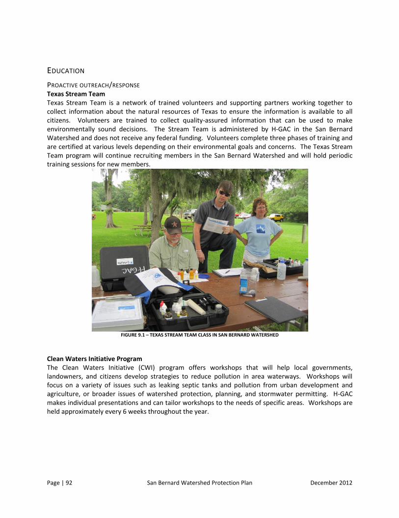
Page | 92 San Bernard Watershed Protection Plan December 2012
EDUCATION
PROACTIVE OUTREACH/RESPONSE Texas Stream Team Texas Stream Team is a network of trained volunteers and supporting partners working together to collect information about the natural resources of Texas to ensure the information is available to all citizens. Volunteers are trained to collect quality-assured information that can be used to make environmentally sound decisions. The Stream Team is administered by H-GAC in the San Bernard Watershed and does not receive any federal funding. Volunteers complete three phases of training and are certified at various levels depending on their environmental goals and concerns. The Texas Stream Team program will continue recruiting members in the San Bernard Watershed and will hold periodic training sessions for new members.
FIGURE 9.1 – TEXAS STREAM TEAM CLASS IN SAN BERNARD WATERSHED
Clean Waters Initiative Program The Clean Waters Initiative (CWI) program offers workshops that will help local governments, landowners, and citizens develop strategies to reduce pollution in area waterways. Workshops will focus on a variety of issues such as leaking septic tanks and pollution from urban development and agriculture, or broader issues of watershed protection, planning, and stormwater permitting. H-GAC makes individual presentations and can tailor workshops to the needs of specific areas. Workshops are held approximately every 6 weeks throughout the year.
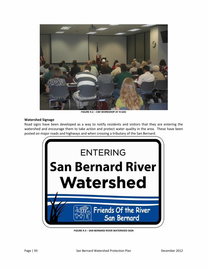
Page | 93 San Bernard Watershed Protection Plan December 2012
FIGURE 9.2 – CWI WORKSHOP AT H-GAC
Watershed Signage Road signs have been developed as a way to notify residents and visitors that they are entering the watershed and encourage them to take action and protect water quality in the area. These have been posted on major roads and highways and when crossing a tributary of the San Bernard.
FIGURE 9.3 – SAN BERNARD RIVER WATERSHED SIGN

Page | 94 San Bernard Watershed Protection Plan December 2012
Texas Watershed Stewards Texas Watershed Stewards (TSW) is a science-based watershed education program designed to help citizens identify and take action to address local water quality impairments. The focus of the group is public participation in local watershed management. The program is open to all watershed residents, including homeowners, business owners, agricultural produces, decision makers, community leaders, and all other citizens. The program has been implemented through the Texas AgriLife Extension Service and The Texas State Soil and Water Conservation Board (TSSWCB) and is now also available online. The goal is to engage as many citizens as possible in the implementation process.
FIGURE 9.4 – TEXAS WATERSHED STEWARDS WORKSHOP
Classroom Presentations The Friends of the River San Bernard has a River Ranger program that presents to local students about the importance of a healthy San Bernard River watershed. The group generally does one program each quarter of the year. Trash Clean Up The Friends of the River San Bernard holds an annual river clean up event each April. They host four collection sites in the tidal portion of the river, where residents can deposit items collected from the river by boat. This clean up event could be extended to the non-tidal portion of the river, particularly in areas where there is a lot of illegal dumping.

Page | 95 San Bernard Watershed Protection Plan December 2012
FIGURE 9.5 – TRASH DUMPED AT A BRIDGE CROSSING ON SAN BERNARD RIVER
WEB SITE The San Bernard Watershed Website is updated and maintained by H-GAC. The website contains information about the watershed, press releases, upcoming meeting announcements, and information presented at previous meetings. There are also links to different types of best management practices (BMPs) along the urban to rural transect and links to sample ordinances on how to reduce nonpoint source pollution. Draft copies of deliverables can also be viewed by downloading them from the website. The URL is www.h-gac.com/go/sanbernard .
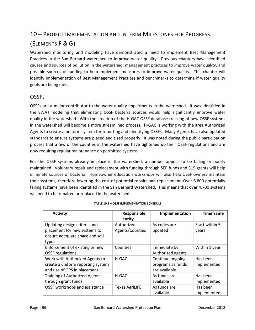
Page | 96 San Bernard Watershed Protection Plan December 2012
10 – PROJECT IMPLEMENTATION AND INTERIM MILESTONES FOR PROGRESS
(ELEMENTS F & G) Watershed monitoring and modeling have demonstrated a need to implement Best Management
Practices in the San Bernard watershed to improve water quality. Previous chapters have identified
causes and sources of pollution in the watershed, management practices to improve water quality, and
possible sources of funding to help implement measures to improve water quality. This chapter will
identify implementation of Best Management Practices and benchmarks to determine if water quality
goals are being met.
OSSFS
OSSFs are a major contributor to the water quality impairments in the watershed. It was identified in
the SWAT modeling that eliminating OSSF bacteria sources would help significantly improve water
quality in the watershed. With the creation of the H-GAC OSSF database tracking of new OSSF systems
in the watershed will become a more streamlined process. H-GAC is working with the area Authorized
Agents to create a uniform system for reporting and identifying OSSFs. Many Agents have also updated
standards to ensure systems are placed and sized properly. It was noted during the public participation
process that a few of the counties in the watershed have tightened up their OSSF regulations and are
now requiring regular maintenance on permitted systems.
For the OSSF systems already in place in the watershed, a number appear to be failing or poorly
maintained. Voluntary repair and replacement with funding through SEP funds and 319 grants will help
eliminate sources of bacteria. Homeowner education workshops will also help OSSF owners maintain
their systems, therefore lowering the cost of potential repairs and replacement. Over 6,800 potentially
failing systems have been identified in the San Bernard Watershed. This means that over 4,700 systems
will need to be repaired or replaced in the watershed.
TABLE 10.1 – OSSF IMPLEMENTATION SCHEDULE
Activity Responsible entity
Implementation Timeframe
Updating design criteria and placement for new systems to ensure adequate space and soil types
Authorized Agents/Counties
As codes are updated
Start within 5 years
Enforcement of existing or new OSSF regulations
Counties Immediate by Authorized agents
Within 1 year
Work with Authorized Agents to create a uniform reporting system and use of GPS in placement
H-GAC Continue ongoing programs as funds are available
Has been implemented
Training of Authorized Agents through grant funds
H-GAC As funds are available
Has been implemented
OSSF workshops and assistance Texas AgriLIFE As funds are available
Has been implemented,

Page | 97 San Bernard Watershed Protection Plan December 2012
Continuous
Voluntary repair and replacement of older systems
Homeowners Through SEP funds Within 1 year
Repair of older systems – county by county
Authorized Agents/counties
Through SEP funds Within 5 years
Connection to existing sewer systems
Cities/counties/homeowners
As funds and systems are available
Within 10 years
TABLE 10.2 – NUMBER OF OSSF REPAIRS NEEDED TO MEET WATER QUALITY STANDARDS
Subbasin Septic
Density (km
-1)
Distance from the Stream
(km)
Subbasin Area (km
2)
Number of Septics/Subbasin potentially failing
How many need to be improved/repaired – to reduce bacteria by 70%
1 5.48 0.422 19.06 104 72.8
2 4.89 0.422 13.01 64 44.8
3 12.40 0.422 7.16 89 62.3
4 13.80 0.422 6.90 95 66.5
5 9.33 0.422 0.45 4 2.8
6 6.16 0.422 14.63 90 63
7 7.78 0.422 4.19 33 23.1
8 10.28 0.422 0.67 7 4.9
9 11.65 0.422 9.13 106 74.2
10 20.05 0.422 6.08 122 85.4
11 17.75 0.422 7.23 128 89.6
12 7.73 0.422 17.58 136 95.2
13 9.53 0.422 3.32 32 22.4
14 15.69 0.422 10.74 169 118.3
15 16.17 0.422 6.39 103 72.1
16 21.41 0.422 1.74 37 25.9

Page | 98 San Bernard Watershed Protection Plan December 2012
17 25.80 0.422 5.19 134 93.8
18 27.63 0.422 3.03 84 58.8
19 16.40 0.422 10.84 178 124.6
20 36.91 0.422 4.13 152 106.4
21 21.88 0.422 5.66 124 86.8
22 18.89 0.422 9.36 177 123.9
23 32.28 0.422 0.96 31 21.7
24 17.82 0.422 3.31 59 41.3
25 17.91 0.422 18.33 328 229.6
26 60.93 0.422 0.54 33 23.1
27 33.69 0.422 7.34 247 172.9
28 19.10 0.422 0.68 13 9.1
29 42.52 0.422 1.12 48 33.6
30 23.26 0.422 1.07 25 17.5
31 33.20 0.422 5.48 182 127.4
32 24.24 0.422 11.35 275 192.5
33 21.21 0.422 9.21 195 136.5
34 10.02 0.422 0.90 9 6.3
35 37.38 0.422 4.32 162 113.4
36 129.31 0.422 3.45 446 312.2
37 77.54 0.422 27.56 2137 1495.9
38 61.05 0.422 4.00 244 170.8
39 51.49 0.422 4.16 214 149.8
40 7.70 0.422 0.14 1 0.7
Highlighted rows indicate sub-watersheds where the geomean exceeds the state standard.

Page | 99 San Bernard Watershed Protection Plan December 2012
WASTEWATER TREATMENT PLANTS/OUTFALLS
Wastewater Treatment Plants are a point source pollution found in the watershed, and their outputs
can be directly measured. At this time, WWTFs in the watershed are not testing the treated wastewater
for bacteria; however they will be as they come under bacteria monitoring requirements when their
permits are renewed. In addition, monitoring bacteria at WWTF outfalls is part of a continued
monitoring program under a 319 (h) grant from the TSSWCB. WWTF bacteria limit testing began about
two years ago to monitor outputs from plants.
In doing the SELECT and SWAT monitoring, it was assumed that their output was at the 126 standard –
which does contribute to the baseline bacteria level in the watershed. However, if their outputs are
lower, this will help lower the baseline bacteria levels. Bacteria monitoring at the wastewater treatment
plant outfalls will help determine if and where bacteria levels need to be lowered. Enforcement of
permits and standards will help keep the baseline levels low as permits are required to be renewed and
will be enforced by TCEQ.
Table 10.4 – WWTF Implementation Schedule
Enforcement Activity Responsible Entity Implementation Timeframe
Testing of effluent for E. coli
WWTF As permits are renewed Within 1 year, as permits are renewed on a 5 year cycle.
Testing of outfalls for E. Coli
H-GAC As part of expanded monitoring program under 319 grant
2 years
TABLE 10.3 - WWTF OUTFALL PERMITS IN THE WATERSHED
Subbasin Name Location Permitted Flow
(MGD)
1 New ULM WSC
WWTF
Bernard RD, 1 mi SE
Intx FM
New ULM, TX 78950
0.05
11 City of Wallis
WWTF
FM RD 1093 & ST
HWY 36
Wallis, TX 77485
0.2
13 Wharton County
WCID No. 2
106 Fitzgerald St.
East Bernard, TX
77435
0.4
21 City of Kendleton
WWTF
1,500 Ft E Farm Market RD 2219
Kendleton, TX
77451
0.08

Page | 100 San Bernard Watershed Protection Plan December 2012
Subbasin Name Location Permitted Flow
(MGD)
22
Hungerford Mud No. 1
WWTF
250 ft NW Int W Live Oak & Haber
Hungerford, TX 77448 0.08
Straightway Inc.
WWTF
Interx FM 1161 & CR 218
Hungerford, TX 77448 0.03
32 City of Needville 14206 Church Street,
Needville, TX 77461 0.4
33 Needville ISD
WWTF
Roesler RD and Danhouse RD,
Needville, TX 77461 0.036
36 Autumn Shadows
WWTF
Sthwy 35, 570 ft East
Sthwy 35
Danbury, TX 77534
0.007
37
City of Sweeny N End of Ave. A on W Bank of
Sweeny, TX 77480 0.975
Bernard Timbers
WSC
USHWY 90A, 1.4M NE
USHWY 90A &
East Bernard, TX 77435
0.021
City of Brazoria
WWTF
One Mile West of
Intersection
Brazoria, TX 77422
0.75
Wild Peach
Elementary WWTF
1 mi S of STHWY 36 @ PT 4.5 mi
S West Columbia, TX 77486 0.01
40 Clemens Unit
WWTF
0.5 mi N Intx St hwy 36
& FM 200
Brazoria, TX 77422
0.54
TABLE 10.4 - SSO OVERFLOWS IN THE WATERSHED
Subbasin WWTF Location SSO Flow
(MGD) Dates of Occurrence
21 City of Kendleton
WWTF
1,500 Ft E Farm Market RD 2219
Kendleton, TX
77451
0.04 5/31/2003
33 Needville ISD
WWTF
Roesler RD and Danhouse RD,
Needville, TX 77461 0.00399428 5/31/2005

Page | 101 San Bernard Watershed Protection Plan December 2012
Subbasin WWTF Location SSO Flow
(MGD) Dates of Occurrence
37
City of Brazoria
WWTF
One Mile West of
Intersection
Brazoria, TX 77422
0.06
0.103
0.04
6/20/2006
12/11/2006
7/3/2007
City of Sweeny N End of Ave. A on W Bank of
Sweeny, TX 77480 4.798 6/2/2002
WILDLIFE/PETS
Wildlife has been identified as a major contributing factor to the bacteria levels in the watershed,
particularly due to the contributions by feral hogs. However, the contribution is not significant enough
to meet the standard if the source were eliminated. Pets are a contributing source, but not considered a
significant source. However the watershed would benefit from a spay/neuter program to help control
feral populations of cats and dogs.
Wildlife contributions are primarily from deer, feral hogs, and other minor sources such as raccoons,
coyotes, opossums, and birds. Deer and feral hog populations were applied to certain land cover areas
in the watershed. Deer populations were applied to pasture and forested areas. Feral hogs were
applied to all land categories except developed areas and open water. Feral hogs are the major
contributor in this category and programs are being implemented statewide to help landowners deal
with the destruction and damage caused by feral hogs.
TABLE 10.5 – WILDLIFE/PETS IMPLEMENTATION SCHEDULE
Activity Responsible Entity Implementation Timeframe
Feral Hog Programs Texas AgriLIFE, Texas Wildlife Service
Ongoing with TWS Have been implemented
Texas AgriLife Extension Service and Texas Wildlife Service workshops for property owners
Landowners Bring programs to the watershed, coordination with AgriLife extension and TWS
Have been implemented
Pork Choppers permitted to hunt hogs in the region
Landowners Ongoing – private contract with landowners
Have been implemented
Pet waste pickup Pet owners Enforcement – municipal codes
Start programs within 2-5 years
Spay and Neuter Program Pet owners City and County programs
Start programs within 2-5 years

Page | 102 San Bernard Watershed Protection Plan December 2012
TABLE 10.6 – DISTRIBUTION OF WILDLIFE IN THE SAN BERNARD WATERSHED BY LAND COVER CATEGORY
Land Cover Category
SUB
W 1
SUB
W 2
SUB
W 3
SUB
W 4
SUB
W 5
SUB
W 6
SUB
W 7
SUB
W 8
SUB
W 9
SUB
W 1
0
High Intensity Developed 0% 0% 0% 0% 0% 0% 0% 0% 1% 0%
Low Intensity Developed 1% 1% 1% 2% 2% 4% 1% 1% 5% 1%
Open Space Developed 0% 0% 0% 0% 0% 0% 0% 0% 2% 1%
Cultivated 62% 87% 89% 85% 77% 68% 47% 60% 26% 7%
Grassland/Shrub 12% 5% 6% 7% 6% 14% 9% 15% 27% 5%
Forest 20% 1% 2% 1% 1% 7% 1% 1% 6% 3%
Woody Wetland 4% 4% 2% 3% 12% 6% 38% 21% 27% 7%
Herbaceous Wetland 1% 1% 1% 1% 1% 1% 2% 1% 4% 70%
Bare 0% 0% 0% 0% 0% 0% 0% 0% 0% 0%
Open Water 0% 0% 0% 0% 0% 0% 1% 0% 2% 6%
LIVESTOCK AND AGRICULTURE
Modeling has identified cattle as a source of concern in the San Bernard Watershed. Agricultural lands
are not a major contributor to the total loadings in the San Bernard watershed; however agricultural
lands do make up the majority of the land cover in the watershed. The TSSWCB also offers Water
Quality Management Plans to landowners in the watershed, and once approved, landowners may be
eligible for funding to help implement the practices identified in the plan. These plans include Best
Management Practices specific to the property help reduce bacteria introduction into area waterways.
Soil testing is also available for landowners to determine the necessary amount of nutrients to apply to
their land.
Currently WQMPs are applied to approximately 10% of the land area in the San Bernard Watershed. In
a survey conducted among watershed residents, there was little knowledge of the availability of these
plans. Advertisement of these plans will help increase implementation in the watershed, and lowering
of bacteria levels associated with livestock and agricultural uses. Additional plans could be added
throughout the watershed – if an additional 1% of the watershed area was added to a WQMP each year,
which would protect an additional 6,800 acres.

Page | 103 San Bernard Watershed Protection Plan December 2012
TABLE 10.7 – LIVESTOCK AND AGRICULTURE IMPLEMENTATION SCHEDULE
Activity Responsible Entity
Implementation Timeframe
Water Quality Management Plans
Landowners TSSWCB Currently implemented
Ag Waste Collection Days (Counties)
Counties, landowners
County by county Within 1 year
Soil Testing to determine the actual amount of nutrients needed
landowners Through AgriLife extension
Already implemented
TABLE 10.8 – DISTRIBUTION OF EXISTING WQMPS IN THE SAN BERNARD WATERSHED
HU
C-1
2
# W
QM
Ps
Acr
eage
un
der
WQ
MP
HU
C-1
2 A
crea
ge
Pre
scri
bed
Gra
zin
g
Nu
trie
nt
Man
age
me
nt
Cro
p R
esid
ue
Man
agem
en
t
Fora
ge H
arve
st
Man
agem
en
t
Wild
life
Lan
d
Co
nse
rvat
ion
Cro
p
Ro
tati
on
%A
cre
age
un
de
r
WQ
MP
120904010101 1 113 30419 113 113 0 0 0 0
0.004
120904010102 0 0 18213 0 0 0 0 0 0
0.000
120904010103 1 109 36802 0 109 0 109 0 0
0.003
120904010104 1 11744 15587 9094 5817 2447 189 5913 2447
0.753
120904010105 1 376 27683 284 375 0 91 0 0
0.014
120904010106 1 1162 14004 1162 1162 0 0 0 0
0.083
120904010107 5 416 15979 1377 1520 105 38 39 105
0.026
120904010108 0 0 26935 0 0 0 0 0 0
0.000
120904010109 16 4377 29444 434 4945 4465 46 40 4465
0.149
120904010201 22 2414 34069 1053 2219 1039 281 14 1039
0.071
120904010202 8 2742 17383 1444 2401 2401 89 5 2401
0.158
120904010204 8 4560 38836 131 4010 2767 1112 505 2767
0.117
120904010203 11 11118 44591 1273 11398 10103 22 168 10103
0.249
120904010205 22 2890 29113 546 2708 1959 203 170 1959
0.099
120904010206 13 448 32892 137 386 82 167 4 82
0.014
120904010207 9 2965 16542 402 2940 2523 15 0 2523
0.179
120904010301 4 280 29696 208 265 0 57 0 0
0.009

Page | 104 San Bernard Watershed Protection Plan December 2012
120904010208 12 2788 31122 841 1941 1276 77 509 1276
0.090
120904010302 4 880 38781 646 433 137 160 0 137
0.023
120904010304 3 2670 26081 1796 1796 0 0 0 0
0.102
120904010303 3 910 35917 757 870 0 113 869 0
0.025
120904010305 2 202 21877 194 194 0 0 0 0
0.009
120904010306 4 878 23236 765 842 0 77 0 0
0.038
120904010307 1 10341 45233 9041 0 0 0 1220 0
0.229
TOTAL 152 64383 680435 31698 46444 29304 2846 9456 29304
10%
LAND MANAGEMENT
Land management in the San Bernard watershed includes a number of BMPs that could be used by land
owners and city and county governments. A number of conservation easements exist in the watershed
along the waterways, conservation easements are a good way for a landowner to preserve their
property and prevent development from occurring adjacent to the waterways. A SEP fund account has
been implemented in the watershed to purchase conservation easements along the San Bernard River.
There are concerns in the watershed about vegetation management along the waterways, some areas
have been clear cut and are eroding, and some are overgrown to the point where water cannot flow.
There are also a number of sites throughout the watershed where trash and appliances have been
dumped off of bridges. There is an annual clean up hosted by the Friends of the River San Bernard to
help combat this program. Currently Counties and Cities lack funding to clean up and monitor these
sites. There is also a lack of sites in which to properly dispose of household hazardous waste, and some
are prohibitively expensive for some residents.
Model ordinances could be used by the jurisdictions in the San Bernard watershed to design nonpoint
source pollution control ordinances or storm water pollution prevention plans. A number of example
ordinances have been collected and posted to the San Bernard Watershed website.
TABLE 10.9 – LAND MANAGEMENT IMPLEMENTATION SCHEDULE
Activity Responsible Entity
Implementation Timeframe
Trash pickup events along waterways
FOR Ongoing, can be expanded/frequency increased
Already implemented
Good Housekeeping/Yardcare in residential areas and neighborhoods
Homeowners Education activities implemented by counties/cities
Already implemented
Conservation Easements to acquire land along waterways
Landowners, FOR
Expand existing programs, use of SEP funds
Already implemented

Page | 105 San Bernard Watershed Protection Plan December 2012
City/County enforcement of illegal dumping and disposal
Cities and counties
By city and county, apply for grants on annual cycle
Within 1 year
Brush management to help in the removal of invasive species to help protect soils, control erosion, reduce sedimentation, and improve water quality
Cities and counties
By county and city
Within 5 years
Identification and removal of abandoned boats
Boaters By county as boats are identified
Immediate
Storm Water Pollution Prevention Plan
Cities and counties
As cities/counties create Updated every 2-5 years
Non Point Source Pollution Control Ordinance
Cities and counties
As cities/counties create Updated every 2-5 years
Stakeholders participated in a survey in order to rank their priorities for implementing BMPs in the
watershed. Stakeholders were asked to rank the BMPs below 1 through 10, 1 being their top priority
and 10 being the lowest. Below are the aggregated results of this survey, the right hand column shows
the average rank that each of the BMPs received. The overwhelming majority of stakeholders ranked
public education and involvement programs as their highest priority. Other BMPs that ranked high
included: repair and replacement of OSSFs, enforcement and testing of WWTFs, and feral hog programs.
These BMPs will be prioritized for implementation and have already been started in the watershed.
TABLE 10.10 – RESULTS OF STAKEHOLDER SURVEY OF BMP IMPLEMENTATION PRIORITIES
Activity Avg.
Public Education and Involvement Programs 2.85
Cattle Management Plans 5.67
Crop Management Plans 7.08
Waste Collection Days (ag, appliances, haz) 5.00
Feral Hog Programs 4.69
Pet Management Programs 9.00
Enforcement and Testing at WWTF 4.15
Repair and Replacement of old OSSFs 4.08
Filter strips surrounding waterways 6.77
Connecting homes to sewer systems 5.00

Page | 106 San Bernard Watershed Protection Plan December 2012
11 – WATER QUALITY MONITORING AND MEASURES OF SUCCESS (ELEMENTS H
& I) H-GAC has received a 319(h) grant from the Texas State Soil and Water Conservation Board to do
additional monitoring in the San Bernard Watershed. This grant includes adding additional quarterly
monitoring sites, increasing some sites to monthly monitoring, wet weather monitoring, and monitoring
of WWTFs in the watershed. This project will help stakeholders monitor the water quality of the
watershed after completion of the Watershed Protection Plan. Monitoring conducted by the H-GAC and
TCEQ will continue on a quarterly basis.
PROJECT GOALS
1. Generate data of known and acceptable quality for surface water quality monitoring of
mainstream, tributary, and WWTF stations
2. Support the implementation of the San Bernard River WPP by collecting water quality data for
use in evaluating the overall effectiveness of BMP implementation, and in assessing progress in
achieving restoration
3. Communicate water quality conditions to the public to support adaptive management of the
San Bernard River WPP
MEASURES OF SUCCESS
Data of known and acceptable quality are generated for surface water quality monitoring of
mainstream, tributary, and WWTF stations
Water quality data is used to evaluate progress in implementing the San Bernard River WPP
Water quality data is communicated to the public and the San Bernard River watershed
stakeholders
Increased watershed stewardship among San Bernard River watershed stakeholders
PROJECT DESCRIPTION
This project will gather further monitoring data for the San Bernard River. This will help stakeholders
determine the improvements of water quality as a benefit of implementing BMPs laid out in the WPP.
Implementation activities for the watershed include: agricultural BMPs for row cropping and cattle
grazing lands, OSSF BMPs for areas of possibly failing systems, and monitoring of post-implementation
activities. The implementation phase will continue the stakeholder involvement from the WPP. Progress
will be assessed by ambient and post-implementation monitoring.
There are currently 8 monitoring stations in the San Bernard Watershed. Five are located along the main
stem of the San Bernard River and 3 are located on tributaries. Three of the stations are monitored by
TCEQ and the other five are monitored by the H-GAC Clean Rivers Program. All eight sites are currently
monitored only once per quarter year. Through this project, H-GAC, in conjunction with EIH, will conduct

Page | 107 San Bernard Watershed Protection Plan December 2012
routine ambient monitoring at the 8 current monitoring stations twice per quarter and an additional 4
sites once per month over 21 months, collecting field, conventional, flow, and bacteria parameter
groups. This will result in routine monitoring being conducted monthly at 12 sites.
H-GAC, in conjunction with EIH, will conduct biased flow monitoring at 15 sites once per season under
wet weather conditions over 7 seasons, collecting field, conventional, flow, and bacteria parameter
groups. Spatial, seasonal and meteorological variation will be captured in these snapshots of watershed
water quality.
If self-reported data is not sufficient to characterize the point source contributions to loadings in the
watershed, H-GAC, in conjunction with EIH, will conduct quarterly effluent monitoring at up to 5 WWTFs
collecting field, conventional, flow, bacteria, and effluent parameter groups.
Collected data will be assessed for trends and variability, effectiveness of implementing BMPs, and
interim short-term progress in achieving water quality goals in the WPP.
PROPOSED ADDITIONAL MONITORING SITES
FIGURE 11.1 ADDITIONAL MONITORING SITES

Page | 108 San Bernard Watershed Protection Plan December 2012
MONTHLY AMBIENT MONITORING
H-GAC, in conjunction with EIH, will conduct routine ambient monitoring at 4 sites once per month and
at 8 sites twice per quarter year, collecting field, conventional, flow, and bacteria parameters groups.
The sampling period extends over 21 months. The number of samples planned for collection through
this subtask is 196.
Currently, routine ambient monitoring is conducted quarterly at 5 stations by H-GAC (16370, 20721,
20722, 20723, and 20460) and at 3 stations by TCEQ (12146, 16373, and 12147) through the Clean
Rivers Program; H-GAC will work with TCEQ to avoid duplicative routing ambient monitoring at these
stations. Sampling through this subtask will complement existing routine ambient monitoring regimes
such that routine water quality monitoring is conducted monthly at 12 sites in the San Bernard River
watershed. H-GAC will contract with an accredited laboratory who will conduct sample analysis.
Field parameters are pH, temperature, conductivity, and dissolved oxygen. Conventional parameters are
total suspended solids, turbidity, sulfate, chloride, nitrate+nitrite nitrogen, ammonia nitrogen, total
kjeldahl nitrogen, chlorophyll-a, total hardness, orthophosphorus and total phosphorus. Flow
parameters are flow collected by gage, electric, mechanical or Doppler, including severity. Bacteria
parameters are E. coli enumerated using Standard Methods (21st Edition) 9223 B, “Enzyme Substrate
Test” and Enterococcus (both for tidal and above tidal sites).
TABLE 11.1 – MONTHLY AMBIENT MONITORING SITES
Site No. Collecting Entity Site ID Site Description
1 HG 16370
San Bernard River immediately downstream of FM
3013 on the Colorado-Austin County Line
approximately 15 KM SW of Sealy
1 EIH 16370
San Bernard River immediately downstream of FM
3013 on the Colorado-Austin County Line
approximately 15 KM SW of Sealy
2 HG 20721 West Bernard Creek at Wharton CR 225 east of
Hungerford
2 EIH 20721 West Bernard Creek at Wharton CR 225 east of
Hungerford

Page | 109 San Bernard Watershed Protection Plan December 2012
3 HG 20722
Peach Creek at Wharton CR 117/Chudalla Road/
Archer Road 89 meters south of the intersection of
Wharton CR 117/ Chudalla Road/ Archer Road and
Wharton CR 212/ Wharton CR 119/ Donaldson Road
East of Wharton
3 EIH 20722
Peach Creek at Wharton CR 117/Chudalla Road/
Archer Road 89 meters south of the intersection of
Wharton CR 117/ Chudalla Road/ Archer Road and
Wharton CR 212/ Wharton CR 119/ Donaldson Road
East of Wharton
4 HG 20723
Mound Creek at Brazoria CR 450/ Jackson
Settlement Road 1.22 KM upstream of FM 1301
west of West Columbia
4 EIH 20723
Mound Creek at Brazoria CR 450/ Jackson
Settlement Road 1.22 KM upstream of FM 1301
west of West Columbia
5 HG 20460 San Bernard River Tidal at SH 35 southwest of West
Columbia
5 EIH 20460 San Bernard River Tidal at SH 35 southwest of West
Columbia
6 FO 12146 San Bernard River Tidal east bank immediately
upstream of FM 2611
6 EIH 12146 San Bernard River Tidal east bank immediately
upstream of FM 2612
7 FO 16373 San Bernard River immediately downstream of US
90A in East Bernard
7 EIH 16373 San Bernard River immediately downstream of US
90A in East Bernard

Page | 110 San Bernard Watershed Protection Plan December 2012
8 FO 12147 San Bernard River mid channel 60 M downstream of
FM 442 bridge SW of Needville
8 EIH 12147 San Bernard River mid channel 60 M downstream of
FM 442 bridge SW of Needville
9 EIH 2 Texas Gulf Canal at FM 1459
10 EIH 3 Bells Creek at SH 35
11 EIH 9b Clarks Branch at CR 211
12 EIH 10a Gum Tree Branch at CR 252
ADDITIONAL QUARTERLY MONITORING
H-GAC, in conjunction with EIH, will conduct routine ambient monitoring at 15 sites quarterly, collecting
field, conventional, flow and bacteria parameter groups. The sampling period extends through 7
seasons. The number of samples planned for collection through this subtask is 105. Spatial and seasonal
variation will be captured in these snapshots of watershed water quality. H-GAC will contract with an
accredited laboratory who will conduct sample analysis.
TABLE 11.2 – ADDITIONAL QUARTERLY MONITORING SITES
Site No. Collecting Entity Site ID Site Description
1 EIH 1 Unnamed Tributary at 2611
2 EIH 1a Unnamed Tributary at 2611
3 EIH 4a Buffalo Creek at FM 442
4 EIH 4b Cedar Creek at FM 442

Page | 111 San Bernard Watershed Protection Plan December 2012
5 EIH 6 Snake Creek at Moody Rd
6 EIH 6b Snake Creek at Modena School Rd
7 EIH 8 Baughman Slough at CR 129
8 EIH 9 West Bernard Creek at CR 211
9 EIH 9a Sandy Branch at CR 213
10 EIH 10 West Bernard Creek at CR 252
11 EIH 10b Dewberry Branch at CR 252
12 EIH 11a Britt Branch at FM 2919
13 EIH 12a Middle Bernard Creek at CR 291
14 EIH 12b Middle Bernard Creek at …
15 EIH 14 East Bernard Creek at FM 1093
WET WEATHER MONITORING
H-GAC, in conjunction with EIH, will conduct biased-flow monitoring at 27 sites once per season under
wet weather conditions, collecting field, conventional, flow and bacteria parameter groups. The
sampling period extends through 7 seasons. The number of samples planned for collection through this
subtask is 189. Spatial, seasonal and meteorological variation will be captured in these snapshots of
watershed water quality. H-GAC will contract with an accredited laboratory who will conduct sample
analysis.
TABLE 11.3 – WET WEATHER MONITORING SITES
Site No. Collecting
Entity Site ID Site Description
1 EIH 16370
San Bernard River immediately downstream of FM 3013
on the Colorado-Austin County Line approximately 15 KM
SW of Sealy
2 EIH 20721 West Bernard Creek at Wharton CR 225 East of
Hungerford

Page | 112 San Bernard Watershed Protection Plan December 2012
3 EIH 20722
Peach Creek at Wharton CR 117/Chudalla Road/ Archer
Road 89 meters South of the intersection of Wharton CR
117/ Chudalla Road/ Archer Road and Wharton CR 212/
Wharton CR 119/ Donaldson Road East of Wharton
4 EIH 20723 Mound Creek at Brazoria CR 450/ Jackson Settlement Road
1.22 KM upstream of FM 1301 west of West Columbia
5 EIH 20460 San Bernard River Tidal at SH 35 southwest of West
Columbia
6 EIH 12146 San Bernard River Tidal east bank immediately upstream
of FM 2611
7 EIH 16373 San Bernard River immediately downstream of US 90A in
East Bernard
8 EIH 12147 San Bernard River mid channel 60 M downstream of FM
442 bridge SW of Needville
9 EIH 1a Unnamed trib off 2611
10 EIH 9 West Bernard Creek at CR 211
11 EIH 9a Sandy Branch at CR 213
12 EIH 9b Clarks Branch at 211
13 EIH 10a Gum Tree Branch at CR 252
14 EIH 10b Dewberry Branch at CR 252
15 EIH 12a Middle Bernard Creek at CR 289
WWTF MONITORING
H-GAC will compile the last 5 years of self-reported effluent discharge data from TPDES permittees in
the watershed. H-GAC will assess the value of this data with respect to the pollutants of interest in this
project. If self-reported data from TPDES permittees are not sufficient to characterize the point source
contribution to pollutant loading to the waterbody, H-GAC will engage a contractor to conduct effluent

Page | 113 San Bernard Watershed Protection Plan December 2012
monitoring at selected WWTFs (up to 5) once per month collecting field, flow, bacteria, and effluent
parameter groups. Effluent parameters are BOD, CBOD and COD. The sampling period extends over 12
months. The number of samples planned for collection through this subtask is 60. Coordination between
TPDES permittees and the TCEQ Regional Office will be required. Neither H-GAC nor TSSWCB shall
submit WWTF data to TCEQ for use in permit compliance and enforcement; rather, WWTF data will only
be used to estimate pollutant loadings from wastewater discharges and to assist TPDES permittees in
improving management and operations.
TABLE 11.4 – WWTF MONITORING SITES
Site No. Collecting Entity Site ID Site Description
1 EIH WWTF1 Wharton County, WCID, East Bernard, Fitzgerald Street.
2 EIH WWTF2 City of Needville in Fort Bend County, 14206 Church Street.
3 EIH WWTF3 City of Sweeny in Brazoria County, End of Ave A/McKinney/CR
372.
SWQMIS AND WRIM DATA TRANSFER
H-GAC will transfer monitoring data from these activities to TSSWCB for inclusion in the TCEQ SWQMIS
at least quarterly. Data will be transferred in the correct format using the TCEQ file structure, along with
a completed Data Summary, as described in the most recent version of TCEQ Surface Water Quality
Monitoring Data Management Reference Guide. H-GAC will submit Station Location Requests to TCEQ,
as needed, to obtain TCEQ station numbers for new monitoring sites. H-GAC will input monitoring
regime, as detailed in the QAPP, into the TCEQ CMS. Data Correction Request Forms will be submitted to
TSSWCB whenever errors are discovered in data already reported. H-GAC will also transfer data to
TSSWCB in the appropriate format for those monitoring activities at least quarterly. H-GAC will post
monitoring data from to the project website and to the H-GAC Water Resources Information Map
(WRIM) (http://webgis2.h-gac.com/CRPflex/).

Page | 114 San Bernard Watershed Protection Plan December 2012
SAN BERNARD WATERSHED PROTECTION PLAN APPENDICES
SELECT MODEL ASSUMPTIONS
A summary of the assumptions used in the application of the SELECT model in the San Bernard
Watershed is presented next. Assumptions were reviewed with stakeholders for input and suggestions.
These assumptions include:
Effluent concentrations from WWTFs were assumed to be 126 cfu/dL;
Increases in WWTF effluent were considered proportional to households
(HH) growth in urban areas;
Non regulated (installed prior to 1989) and regulated OSSFs systems presented a failure rate of
50% and 12% respectively (Reed, Stowe, and Yanke, 2001);
Increase in the number of OSSFs were considered proportional to households (HH) growth in
rural areas;
New households in rural areas were considered to occupy 1/2 ac per HH and were located in
cultivated, hay/pasture, herbaceous, forest, wetlands, forest and wetlands in proportion (40, 30,
10, 10, and 10%). Livestock were located mainly in herbaceous and 90% of hay/pasture land
cover categories and wildlife were located in forest and wetland areas (Teague, 2009);
Densities of livestock and wildlife were considered to remain constant at current values during
forecast.
A buffer zone of 100 m was delimited around streams. It was assumed that 100% of the
loadings within the buffer and 25% of the loadings outside the buffer reach the streams.
TABEL A.1 LOADING FROM EACH WATERSHED BY SOURCE
SUBW. SUBWATERSHED
OSSFs
WWTF
Urban Runoff
Dogs
Cattle
Deer
Hogs
Horses
Sheep_Goat
SW1 SW1- SB/Little San
Bernard River 8% 0% 11% 2% 23% 28%
16% 17% 11%
SW2 SW2- SB/East Bernard
Creek 8% 8% 12% 8% 21% 18%
13% 24% 18%
SW3 SW3- Middle Bernard
Creek 2% 0% 6% 1% 10% 7% 8% 5% 5%
SW4 SW4- West Bernard Creek 8% 2% 19% 12% 15%
11%
18% 10% 20%
SW5 SW5- SB/Snake Creek 16% 21% 15% 11% 7% 9%
15% 13% 8%
SW6 SW6- Peach Creek 5% 0% 8% 7% 6% 5% 5% 4% 8%
SW7 SW7- SB/Cedar Creek 9% 9% 7% 9% 6% 7% 10% 8% 8%
SW8 SW8- Mound Creek 5% 0% 3% 2% 3% 3% 4% 6% 5%
SW9 SW9- SB/Upper Tidal 34% 60% 18% 45% 6%
11% 9% 13% 16%
SW1 SW10- SB/Lower Tidal 4% 0% 2% 4% 1% 1% 1% 1% 1%

Page | 115 San Bernard Watershed Protection Plan December 2012
0
TABLE A.2 LOADINGS BY SOURCE IN EACH WATERSHED
SUBW. SUBWATERSHED
OSSFs
WWTF
Urban Runoff
Dogs
Cattle
Deer
Hogs
Horses
Sheep_Goat
SW1 SW1- SB/Little San
Bernard River 2% 0% 6% 2% 72% 1% 14% 0% 4%
SW2 SW2- SB/East Bernard
Creek 2% 0% 7% 8% 65% 1% 11% 0% 6%
SW3 SW3- Middle Bernard
Creek 1% 0% 7% 1% 69% 1% 17% 0% 4%
SW4 SW4- West Bernard
Creek 2% 0% 11% 13% 49% 0%
17% 0% 7%
SW5 SW5- SB/Snake Creek 5% 0% 13% 18% 36% 1%
22% 0% 5%
SW6 SW6- Peach Creek 3% 0% 11% 19% 47% 1%
12% 0% 7%
SW7 SW7- SB/Cedar Creek 4% 0% 9% 20% 41% 1%
19% 0% 6%
SW8 SW8- Mound Creek 6% 0% 8% 8% 50% 1% 18% 0% 9%
SW9 SW9- SB/Upper Tidal 7% 0% 10% 47% 20% 0% 8% 0% 6%
SW10 SW10- SB/Lower Tidal 9% 0% 10%
44% 21% 0%
11% 0% 5%
FORECAST OF SOURCES BY 2006 LAND COVER TYPE
The loadings associated with each land cover type have been projected out to the year 2040 in five year
increments based on the projected household population growth in the five counties. Household
forecasts were obtained from the Forecast Group at H-GAC. This data was for urban and rural areas in
five year increments over the period of 30 years. This information was used to project additional
households in the subwatershed which were associated with additional impervious surfaces, OSSFs, and
pets.
TABLE A.3 PERCENTAGE OF EACH SOURCE BY YEAR
SOURCES 2010 2015 2020 2025 2030 2035 2040
OSSFs 3.3% 3.2% 3.1% 2.7% 2.2% 1.6% 1.1%
WWTFs 0.0% 0.0% 0.0% 0.0% 0.0% 0.0% 0.0%
Urban Runoff 8.4% 7.3% 5.9% 4.2% 2.7% 1.6% 0.9%
Dogs 16.0% 14.5% 12.3% 9.6% 6.9% 4.6% 2.8%
Cattle 47.5% 41.3% 32.7% 23.2% 14.7% 8.4% 4.6%

Page | 116 San Bernard Watershed Protection Plan December 2012
Horses 0.2% 0.1% 0.1% 0.1% 0.0% 0.0% 0.0%
Sheep/Goat 5.5% 4.8% 3.8% 2.7% 1.7% 1.0% 0.5%
Livestock 53.2% 46.2% 36.6% 26.0% 16.4% 9.4% 5.1%
Deer 0.6% 0.5% 0.4% 0.3% 0.2% 0.1% 0.1%
Feral Hogs 13.9% 24.1% 38.5% 54.9% 70.1% 81.8% 89.6%
Geese 4.6% 4.0% 3.2% 2.3% 1.5% 0.9% 0.5%
Wildlife Total 19.1% 28.7% 42.1% 57.5% 71.8% 82.8% 90.2%
TOTAL 100% 100% 100% 100% 100% 100% 100%
The results of the forecast model show that cattle will continue to be the highest potential source of
bacteria in the watershed, and OSSFs will continue to be the second highest potential source of bacteria.
As agricultural areas are developed, loadings from livestock and wildlife will be reduced as loadings from
pets rise with the number of households.
TABLE A.4 – NLDC 2006 EC LOADING (CFU/DAY)
NLDC 2006 EC LOADING (CFU/day)
SUBW. SUBWATERSHED
OSSFs
WWTF
Urban Runoff Dogs
Cattle
Horses
Sheep & Goat
Feral Hogs Deer
Geese
SW1 SW1- SB/Little San
Bernard River 1.1E+
12 6.4E+
06 1.3E+12 1.7E+
12 3.9E+
13 9.3E+
10 2.2E+12 7.2E+1
2 6.0E+
11 1.4E+
10
SW2 SW2- SB/East Bernard
Creek 1.1E+
12 7.5E+
08 1.5E+12 3.2E+
12 3.7E+
13 1.3E+
11 3.6E+12 6.5E+1
2 4.1E+
11 5.8E+
10
SW3 SW3- Middle Bernard
Creek 3.3E+
11 0.0E+
00 6.9E+11 5.2E+
11 1.9E+
13 3.0E+
10 1.1E+12 4.3E+1
2 1.6E+
11 6.5E+
11
SW4 SW4- West Bernard
Creek 1.1E+
12 1.9E+
08 2.3E+12 4.1E+
12 2.7E+
13 5.6E+
10 4.1E+12 9.3E+1
2 2.6E+
11 5.0E+
12
SW5 SW5- SB/Snake Creek 2.2E+
12 2.1E+
09 1.8E+12 5.1E+
12 1.5E+
13 7.2E+
10 2.1E+12 8.1E+1
2 2.3E+
11 4.1E+
11
SW6 SW6- Peach Creek 6.4E+
11 0.0E+
00 9.3E+11 2.3E+
12 1.1E+
13 2.2E+
10 1.8E+12 2.7E+1
2 1.2E+
11 0.0E+
00
SW7 SW7- SB/Cedar Creek 1.3E+
12 8.6E+
08 9.1E+11 3.6E+
12 1.1E+
13 4.8E+
10 1.6E+12 5.3E+1
2 1.5E+
11 8.5E+
10
SW8 SW8- Mound Creek 7.2E+
11 0.0E+
00 3.5E+11 1.2E+
12 6.7E+
12 3.6E+
10 1.2E+12 2.2E+1
2 9.1E+
10 0.0E+
00
SW9 SW9- SB/Upper Tidal 4.7E+
12 5.9E+
09 2.3E+12 1.6E+
13 1.1E+
13 7.4E+
10 3.3E+12 4.9E+1
2 2.6E+
11 2.0E+
10
SW10 SW10- SB/Lower Tidal
4.9E+11
0.0E+00 2.0E+11
1.4E+12
1.4E+12
7.5E+09 3.3E+11
8.0E+11
2.7E+10
5.3E+11
TOTAL TOTAL
1.4E+13
9.8E+09 1.2E+13
3.9E+13
1.8E+14
5.7E+11 2.1E+13
5.1E+13
2.3E+12
6.8E+12
MODEL CALIBRATION
Model calibration is the process where the model input parameters are adjusted until the simulated
data from the model match with observed data. Model inputs and parameters (as identified in this
section) related to watershed/landscape processes were adjusted to match the measured and simulated
flow, sediment, and nutrients at key locations in the watershed. During the calibration process, model
parameters will be adjusted within literature recommended ranges or based on site-specific
Page | 117 San Bernard Watershed Protection Plan December 2012
considerations as appropriate. Model calibration is an iterative procedure that is achieved using a
combination of best professional judgment and quantitative comparison with a subset of the measured
data.
Model parameters for both the SWAT and Tidal Prism Models were adjusted to minimize differences
between measured and simulated flow and water quality trends at key locations. All model parameters
will be adjusted within reasonable ranges recommended in published literature or based on site-specific
considerations.
WATERSHED MODEL – SWAT
MODEL SETUP
The first task was to compile and review available physical, water quality and source data for the system.
This evaluation included the water quality data at all eight monitoring sites, flow data from the USGS
gauge in the San Bernard River watershed (USGS gage number 08117500), local meteorological data,
land cover data, and topographic information. With data compiled, the next step was to set up the
watershed model and the stream model, using the available topographic information.
WATERSHED DELINEATION
The watershed delineation for the San Bernard River, as outlined in the project QAPP, was proposed to
be based on the boundaries used for the SELECT modeling. However, there were several streams that
were not adequately represented in the SELECT model that warranted additional refinement of the
subbasins. Additionally, the SELECT subbasins were not aligned with monitoring station in the
watershed. Therefore, the subbasins were redelineated using the SWAT automatic delineation process.
The automatic delineation requires input a Digital Elevation Model (DEM), which for the San Bernard
River was based on the USGS National Elevation Dataset (NED). During the automatic delineation
process, the model identifies stream segments and calculates flow direction and accumulation. Each
subbasin contains only one reach and the length is determined by the subbasins boundary. The DEM
used for watershed delineation is presented in Figure 5.6.
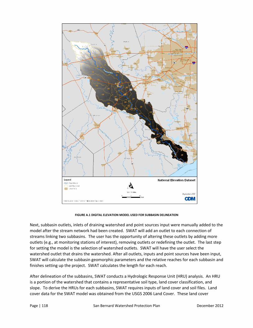
Page | 118 San Bernard Watershed Protection Plan December 2012
FIGURE A.1 DIGITAL ELEVATION MODEL USED FOR SUBBASIN DELINEATION
Next, subbasin outlets, inlets of draining watershed and point sources input were manually added to the
model after the stream network had been created. SWAT will add an outlet to each connection of
streams linking two subbasins. The user has the opportunity of altering these outlets by adding more
outlets (e.g., at monitoring stations of interest), removing outlets or redefining the outlet. The last step
for setting the model is the selection of watershed outlets. SWAT will have the user select the
watershed outlet that drains the watershed. After all outlets, inputs and point sources have been input,
SWAT will calculate the subbasin geomorphic parameters and the relative reaches for each subbasin and
finishes setting up the project. SWAT calculates the length for each reach.
After delineation of the subbasins, SWAT conducts a Hydrologic Response Unit (HRU) analysis. An HRU
is a portion of the watershed that contains a representative soil type, land cover classification, and
slope. To derive the HRUs for each subbasins, SWAT requires inputs of land cover and soil files. Land
cover data for the SWAT model was obtained from the USGS 2006 Land Cover. These land cover

Page | 119 San Bernard Watershed Protection Plan December 2012
classifications were aligned with SWAT classifications as shown in Table 5.17. The land cover dataset
used for HRU analysis is presented in Figure 5.7 and the relative areas of land covers within the model
are presented in Table 5.18.
TABLE A.5 LAND COVER ASSIGNMENTS FOR SWAT
HGAC Class Classification
Open Water WATR
Developed, Low Intensity URLD
Developed, Medium Intensity URMD
Deciduous Forest FRSD
Evergreen Forest FRSE
Mixed Forest FRST
Shrub/ Scrub RNGB
Herbaceous RNGE
Hay/Pasture HAY
Cultivated Crops AGRR
Emergent Herbaceous Wetlands WETF
Woody Wetlands WETN
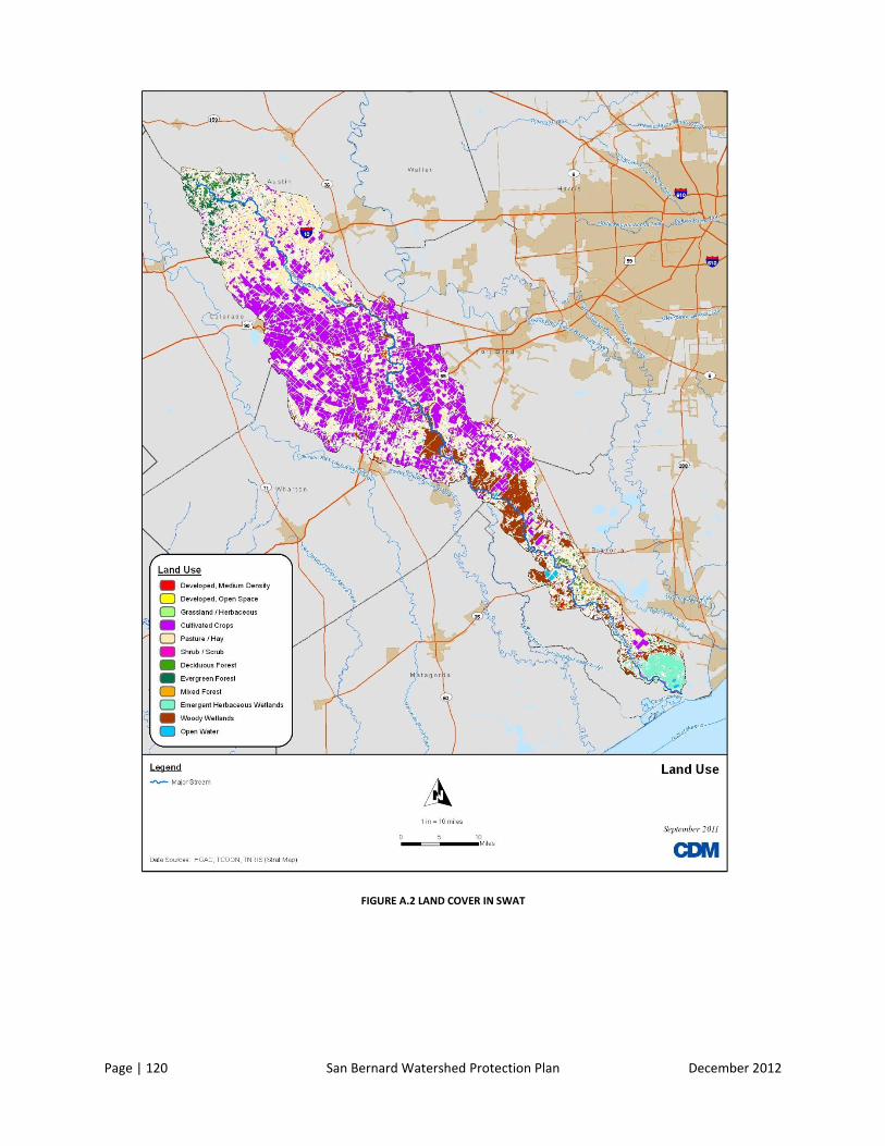
Page | 120 San Bernard Watershed Protection Plan December 2012
FIGURE A.2 LAND COVER IN SWAT

Page | 121 San Bernard Watershed Protection Plan December 2012
Soils for the HRU analysis were based on the State Soil Geographic Database (STATSGO) soils dataset
available from USEPA through their BASINS datasets. Soil data were classified based on the STATSGO
polygon number (i.e., MUID) to link the dataset to the U.S. Soils database within SWAT and then
imported in the SWAT model. The soils dataset used for HRU analysis is presented in Figure 5.8 and is
summarized in Table 5.19.
TABLE A.6 LAND COVER DISTRIBUTION IN SWAT
Land cover Area (hectares) Percentage
AGRR 87570.57 36.4%
FRSD 7172.578 3.0%
FRSE 7032.947 2.9%
FRST 24.39151 0.0%
HAY 85294.46 35.4%
RNGB 8666.688 3.6%
RNGE 28.0254 0.0%
URLD 4444.126 1.8%
URMD 89.40324 0.0%
WATR 625.8691 0.3%
WETF 33383.01 13.9%
WETN 6457.821 2.7%
Grand Total 240789.9 100.0%
TABLE A.7 SOILS INCLUDED IN THE SWAT MODEL
Soil Type Major Soil Component Area (hectare) Percentage Curve Number Range
TX031 Asa 2839.38 1% 54 - 61
TX162 Edna 1012.45 0% 74 - 78
TX163 Edna 22172.06 9% 72 - 84
TX185 Francitas 1449.66 1% 79 - 79
TX220 Harris 2820.74 1% 75 - 87
TX249 Katy 12895.77 5% 74 - 84
TX276 Lake Charles 34767.71 14% 74 - 87
TX277 Lake Charles 12256.73 5% 74 - 84
TX356 Nada 53565.36 22% 74 - 84
TX423 Pledger 38558.42 16% 72 - 87
TX539 Surfside 3609.70 1% 74 - 87
TX550 Telferner 14330.38 6% 74 - 84
TX571 Tremona 10207.62 4% 65 - 72
TX618 Wockley 30303.92 13% 65 - 80
Total 240789.8897 100% 54 - 87
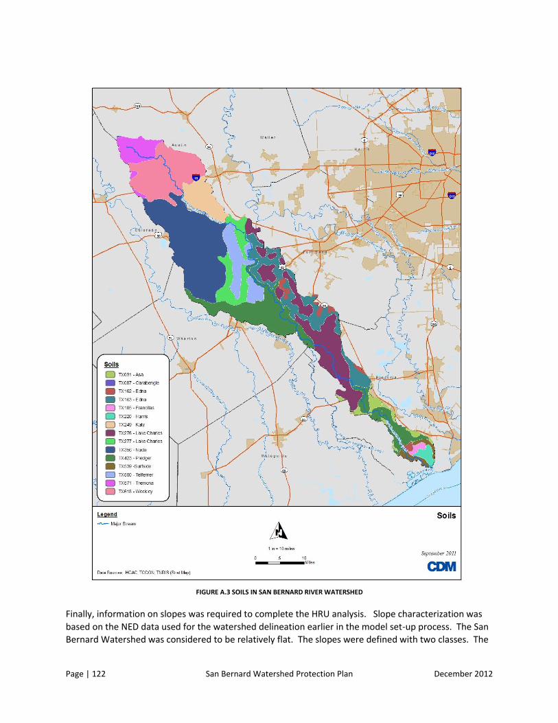
Page | 122 San Bernard Watershed Protection Plan December 2012
FIGURE A.3 SOILS IN SAN BERNARD RIVER WATERSHED
Finally, information on slopes was required to complete the HRU analysis. Slope characterization was
based on the NED data used for the watershed delineation earlier in the model set-up process. The San
Bernard Watershed was considered to be relatively flat. The slopes were defined with two classes. The
Page | 123 San Bernard Watershed Protection Plan December 2012
first class ranged from 0 to 1 percent and the second class ranged greater than 1 percent. The slope
dataset used for HRU analysis is presented in Figure 5.9.
To define an individual HRU, SWAT requires that thresholds be established for each data type. For
example, a threshold of 25 percent for land cover would mean that any land cover within the watershed
having less than 5 percent total area would not be included as one of the key land cover types within
that HRU. The threshold for the land cover was set to 5 percent over the subbasin area. The soil
threshold was set to 25 percent and the slope threshold was set to 20 percent. After the thresholds
were established, the model calculated the appropriate HRUs for each subbasin and populated the
model files with default values.
Weather Data
The SWAT model requires several key pieces of weather data including precipitation, temperature, as
well as humidity, wind speed and direction. Weather data for the simulation was collected from five
weather stations in and around the San Bernard Watershed: Brenham, Bellville, Wharton, Wharton
Airport, and Freeport. Specific information on each type of weather data is provided in more detail
subsequently.
Although precipitation data were collected from the five stations noted previously, three stations
(Bellville, Wharton, and Freeport) are located closest to the watershed. Therefore, data from these
three stations were used preferentially to generate most of the precipitation input for SWAT. If there
were gaps in the data during the simulation period the other two stations were used to complete these
gaps. During the review of the weather data, one key discrepancy was noted for the precipitation data
collected for Wharton County. One value noted on July 27, 2008 was noted to have a total of 13.98
inches of rainfall occurring but it could not be verified with other data sources such as NOAA, nearby
weather stations. As such, it was removed from the rainfall dataset. A graph of the precipitation data is
shown in Figure 5.10; a map of the subbasins assigned to each gage is presented in Figure 5.11.

Page | 124 San Bernard Watershed Protection Plan December 2012
FIGURE A.4 SLOPES IN SAN BERNARD WATERSHED

Page | 125 San Bernard Watershed Protection Plan December 2012
FIGURE A.5 PRECIPITATION FOR 3 RAINFALL GAGES IN MODEL

Page | 126 San Bernard Watershed Protection Plan December 2012
FIGURE A.6 PRECIPITATION GAGES ASSIGNED BY BASIN

Page | 127 San Bernard Watershed Protection Plan December 2012
The temperature data were collected from the Freeport, Brenham, and the Wharton airport stations.
For the model the temperature stations were set up in Freeport and Wharton. The only gage that had
relative humidity and wind data for the entire period of modeling was the station located in Wharton.
SWAT has the ability to calculate a few of weather parameters such as solar radiation and
evapotranspiration. Some of the chosen gages did not contain any information on solar radiation and
evapotranspiration and the gages that did had data for the parameters had very little data. Therefore,
the SWAT model was used to generate both of these parameters. The Penham-Monteith Equation was
used to calculate evapotransportation. Plots of both the SWAT-generated solar radiation and
evapotranspiration are presented in Figure 12 and 13.
FIGURE A.7 EVAPOTRANSPIRATION GENERATED BY SWAT

Page | 128 San Bernard Watershed Protection Plan December 2012
FIGURE A.8 EVAPOTRANSPIRATION GENERATED BY SWAT
HYDROLOGY SET-UP AND CALIBRATION APPROACH
Upon set-up, the SWAT model is populated with default values based upon the information provided in
the soils, DEM, land cover and slope data sets. The hydrologic balance of SWAT is largely based on
several “reservoirs” of water including precipitation, infiltration, surface runoff, lateral flow,
evapotranspiration, percolation and transmission losses that are simulated in four control volumes:
surface runoff, soil profile or root zone, shallow aquifer and deep aquifer (Neitsch, S.L., Arnold, J.G.,
Kiniry, J.R.., Srinivasan, R, and Williams, J.R., 2010).
For the purposes of the San Bernard watershed, the model was set up to simulate daily flows based on
the Curve Number method. These daily flows were compared to the USGS gage at USGS ID 08117500
(San Bernard River near Boling, Texas) which reports flow from 1954 to now. The Lower Colorado River
Authority also maintains a gage in the upper portion of the San Bernard River. This gage was not used in
the calibration process because the data quality could not be verified.
There were several sensitive parameters within the hydrology portion of the model. One of the key
sensitive parameters in the model was the Curve Number. The curve numbers were established in
SWAT based on the soil type and land cover specified for each hydrologic unit. The curve numbers were
calibrated within a range of +/- 5 to achieve the best fit for the flow simulation as will be discussed
subsequently. A table of curve numbers used in the model is presented in Table 5.20.
0
5
10
15
20
25
30
0 2 4 6 8 10 12 14
Sola
r R
adia
tio
n (
MJ/
m2/d
ay)
Date (month)
Subbasin 3
Subbasin 38

Page | 129 San Bernard Watershed Protection Plan December 2012
TABLE A.8 CURVE NUMBERS ESTABLISHED BY SUBBASIN
Subbasin
Initial Curve Number
Minimum Maximum
1 65 72
2 65 72
3 67 84
4 67 84
5 74 84
6 65 84
7 67 84
8 74 84
9 74 84
10 74 84
11 74 84
12 74 84
13 74 84
14 74 84
15 74 84
16 74 84
17 74 84
18 74 84
19 74 84
20 74 84
21 74 84
22 74 84
23 74 84
24 74 84
25 74 84
26 78 84
27 74 84
28 74 84
29 74 84
30 74 84
31 74 84
32 74 84
33 74 84
34 72 84
35 74 84
36 74 87
37 54 78
38 54 79
Subbasin
Initial Curve Number
Minimum Maximum
39 74 87
40 75 87

Nine Element Table
Page | 130 San Bernard Watershed Protection Plan December 2012
Other key parameters that were found to be sensitive in the model were the following:
SURLAG, which is surface runoff lag coefficient, was set to 2.0. This value is treated as a calibration
parameter; larger values of SURLAG will result in surface runoff being generated more quickly from
the watershed and in greater amounts;
ESCO, which is the soil evaporation compensation factor, was set to 0.25. This is the maximum
value for ESCO. As the value for ESCO increases, the model extracts less evaporative demand from
lower soil levels.
EPCO, which is the plant uptake compensation factor, was set to 0.0 which is the minimum value for
EPCO. As EPCO approaches 0, the model allows less water update demand to be met by lower
layers of the soil.
ALPHA_BF, which is the baseflow alpha factor, was set to 0.9. ALPHA_BF is a key factor in
controlling the baseflow recession in SWAT.
The above parameters were treated as calibration coefficients in the model and adjusted to achieve the
best fit with the model output to the observed data from the USGS gage as will be described in the next
section.
HYDROLOGY MODEL PERFORMANCE
A calibration period of up to two years was selected as per the project Quality Assurance Project Plan
(QAPP), with representative weather conditions that contain a reasonable amount of monitoring data.
Additionally, the simulation period excludes the first year of the SWAT simulation to allow the model
hydrologic “reservoirs” time to “spin-up” and come to equilibrium. Therefore, the simulation period use
for the SWAT model was from January 1, 2001 through December 31, 2005. The first year of the SWAT
simulation was not included in the calibration period to allow the model adequate “spin-up” time, which
is standard practice for SWAT and other hydrologic modeling approaches. A validation period was also
selected to assess how well the model was performing on data that were not used to calibrate the
model. The validation period was January 1, 2005 through September 30, 2009.
Model performance was evaluated on the basis of several criteria including:
Annual and seasonal flow volume comparisons;
Cumulative frequency distributions of observed and simulated flows; and
Time series plots of observed and simulated flows.
The results from the modeling are presented in Table 5.21 for the calibration period. As can be seen
from the table, the model performance can be considered “good” and the hydrology validation “very
good” based upon typical calibration guidelines (Donigian et al., 2002).
TABLE A.9 HYDROLOGY PERFORMANCE TABLE (VOLUMES IN CUBIC METERS)
Data
Source
Simulation
Period
Total
Volume
90th
Percentile
10th
Percentile
30th
Percentile
Summer
Volume
Observed Calibration Period 2.78E+09 3.17E+09 1.10E+07 7.77E+07 6.31E+08
Validation Period 1.50E+09 3.57E+06 3.21E+04 1.07E+05 4.73E+08
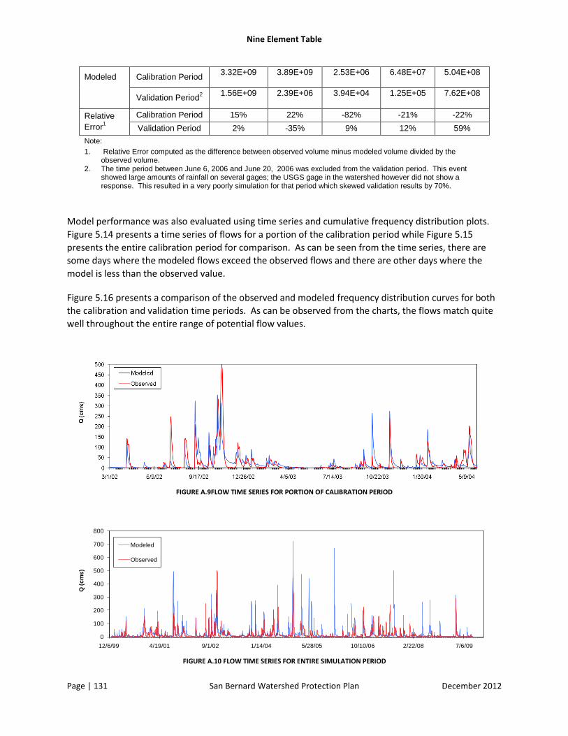
Nine Element Table
Page | 131 San Bernard Watershed Protection Plan December 2012
Modeled Calibration Period 3.32E+09 3.89E+09 2.53E+06 6.48E+07 5.04E+08
Validation Period
2
1.56E+09 2.39E+06 3.94E+04 1.25E+05 7.62E+08
Relative
Error1
Calibration Period 15% 22% -82% -21% -22%
Validation Period 2% -35% 9% 12% 59%
Note:
1. Relative Error computed as the difference between observed volume minus modeled volume divided by the observed volume.
2. The time period between June 6, 2006 and June 20, 2006 was excluded from the validation period. This event showed large amounts of rainfall on several gages; the USGS gage in the watershed however did not show a response. This resulted in a very poorly simulation for that period which skewed validation results by 70%.
Model performance was also evaluated using time series and cumulative frequency distribution plots.
Figure 5.14 presents a time series of flows for a portion of the calibration period while Figure 5.15
presents the entire calibration period for comparison. As can be seen from the time series, there are
some days where the modeled flows exceed the observed flows and there are other days where the
model is less than the observed value.
Figure 5.16 presents a comparison of the observed and modeled frequency distribution curves for both
the calibration and validation time periods. As can be observed from the charts, the flows match quite
well throughout the entire range of potential flow values.
FIGURE A.9FLOW TIME SERIES FOR PORTION OF CALIBRATION PERIOD
FIGURE A.10 FLOW TIME SERIES FOR ENTIRE SIMULATION PERIOD
0
100
200
300
400
500
600
700
800
12/6/99 4/19/01 9/1/02 1/14/04 5/28/05 10/10/06 2/22/08 7/6/09
Q (
cm
s)
Modeled
Observed
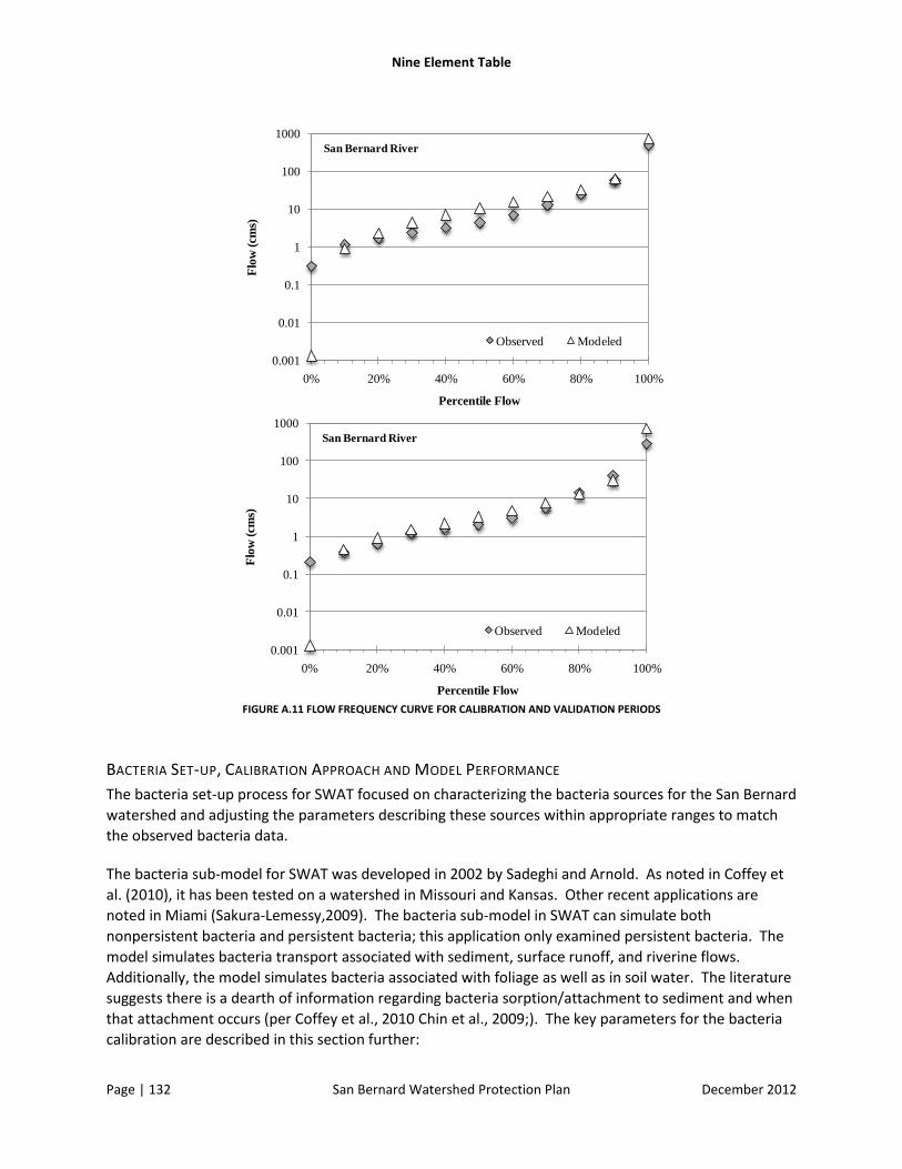
Nine Element Table
Page | 132 San Bernard Watershed Protection Plan December 2012
FIGURE A.11 FLOW FREQUENCY CURVE FOR CALIBRATION AND VALIDATION PERIODS
BACTERIA SET-UP, CALIBRATION APPROACH AND MODEL PERFORMANCE
The bacteria set-up process for SWAT focused on characterizing the bacteria sources for the San Bernard
watershed and adjusting the parameters describing these sources within appropriate ranges to match
the observed bacteria data.
The bacteria sub-model for SWAT was developed in 2002 by Sadeghi and Arnold. As noted in Coffey et
al. (2010), it has been tested on a watershed in Missouri and Kansas. Other recent applications are
noted in Miami (Sakura-Lemessy,2009). The bacteria sub-model in SWAT can simulate both
nonpersistent bacteria and persistent bacteria; this application only examined persistent bacteria. The
model simulates bacteria transport associated with sediment, surface runoff, and riverine flows.
Additionally, the model simulates bacteria associated with foliage as well as in soil water. The literature
suggests there is a dearth of information regarding bacteria sorption/attachment to sediment and when
that attachment occurs (per Coffey et al., 2010 Chin et al., 2009;). The key parameters for the bacteria
calibration are described in this section further:
0.001
0.01
0.1
1
10
100
1000
0% 20% 40% 60% 80% 100%
Flo
w (cm
s)
Percentile Flow
Observed Modeled
San Bernard River
0.001
0.01
0.1
1
10
100
1000
0% 20% 40% 60% 80% 100%
Flo
w (cm
s)
Percentile Flow
Observed Modeled
San Bernard River
Nine Element Table
Page | 133 San Bernard Watershed Protection Plan December 2012
Manure loading: One of the key components simulated in the SWAT model is manure loading on
the land surface from grazing livestock and continuous deposition for livestock. For livestock
grazing, the dry weight of manure deposited daily (MANURE_KG) was specified for each HRU
associated with Hay and Range land covers. Continuous deposition of fertilizer (i.e., manure) and
bacteria associated with the manure (BACTPDB)) and continuous deposition by wildlife. This was
specified using the range of values presented in Tables 5.15 and 5.16 above and the
wildlife/livestock/domestic pet estimates based on information from the National Agricultural
Census and other sources in the watershed. In some cases, the amount of manure loading was
adjusted outside these ranges in order to calibrate the model. These “unknown” sources were
assigned to the manure loading category based on knowledge that livestock and wildlife estimates
in the watershed were based on county-wide data and may not have captured the true number of
animals within the San Bernard River basin. Therefore, in order to calibrate the model, the
watershed loading from the animals was adjusted to best represent long-term geometric mean
concentrations in the watershed.
Bacteria die-off coefficients: As noted previously, SWAT can simulate bacteria on foliage, soil,
associated with sediment and in-streams. Die-off coefficients are specified for all of these
conditions in the model. For the San Bernard River modeling effort, die-off coefficients for bacteria
were set as follows: on foliage (WDPF) set to 0.04 per day; in soil solution (WDPQ) set to 0.4 per
day, adsorbed to soil particles (WDPS) set to 0.04 per day, and in-stream associated with moving
water (WDPRCH) set to 0.3 per day. These values are within the typical range reported for these
parameters in the SWAT modeling literature.
Bacteria soil partitioning coefficient (BACTKDQ): This value is the ratio of the bacteria
concentration in the surface 10 mm of soil water to the concentration of bacteria in surface runoff.
Higher values result in lower concentrations of bacteria in the surface runoff. The value for the San
Bernard watershed was set to 175; this default value has been found to be appropriate in several
other SWAT modeling applications.
Bacteria percolation coefficient (BACTMIX): The bacteria percolation coefficient is the ratio of
bacteria concentrations in the top 10 mm of soil to the concentration of bacteria in the percolate.
The model default value is 10.0 and the value can range from 7.0 to 20.0. The value for the San
Bernard watershed was set to 10.0 based on other studies that have applied the default value.
The above parameters were treated as calibration coefficients in the model and adjusted to achieve the
best fit with the model output to the observed data from the Clean Rivers Program and TCEQ
monitoring stations within the watershed, with the focus on long-term geometric mean concentrations
at each station.
RECEIVING WATER MODEL
To simulate bacteria in the tidal portion of the watershed, a time-variable tidal prism model was
developed in Microsoft Excel for the same simulation period as the SWAT model, January 1, 2007
through September 1, 2009. The tidal prism model was developed to simulate in-stream loading in the
tidal portion of the San Bernard River by taking into account the volume of water that is carried
upstream by the tidal fluctuations. Also included in the tidal model are runoff inputs from the SWAT
model, WWTF discharges, and SSO discharges.

Nine Element Table
Page | 134 San Bernard Watershed Protection Plan December 2012
The model segmentation in the tidal prism model was based on 2-mile long sections along the length of
the tidal portion of the river, for a total of 16 segments. The model segmentation is presented in Figure
5.17.
MODEL SET-UP – HYDRAULICS
The change in volume associated with change in water level as a result of tidal fluctuations is a critical
component that must be accounted for in the tidal prism model. Because cross-section data were not
available in the lower portion of the San Bernard River, volume estimates were generated based on
simple trapezoidal cross-sections. The top-width of the cross-sections were established based on
measurements taken from Google Earth elevation data. These cross-sections, while not detailed,
provide the best available data upon which to base the volume calculations. The San Bernard River is
divided into a tidal and non-tidal portion by a salt water barrier dam. The Tidal Prism Model was used to
determine tidal fluctuations in the tidal part of the watershed.
To define the volumes, the first step was to define a tidal boundary condition. For the San Bernard River
model, the tidal boundary was developed using tide data from the Texas Coastal Ocean Observation
Network (TCOON) from the United States Coast Guard (USCG) Station at Freeport near Surfside Beach
which is shown on Figure 5.18. Tide data at this station were collected from September 2006 through
the present. Although this tide gauge is located 10 miles northeast of the project boundary, it is the
closest tide gage to the watershed and was used as the basis for the tide boundary. Values range from
24.9 ft to 35.1 ft, but there is no datum associated with that monitoring station. The average value of
the tide measurements for this station was assumed to be mean sea level, and values were adjusted to
match accordingly; adjusted values range from -3.9 ft to 6.4 ft. After water levels were determined, they
were used in conjunction with the cross-sectional area, estimated invert elevations from the Google
Earth and length of the segment to calculate the volume at various locations throughout the tidal
portion of the San Bernard River.
The tidal prism model also received flow inputs for WWTF discharges, SSO discharges, upstream
boundary condition from SWAT, and watershed runoff from the SWAT model. These inputs were
included as point sources to each segment of the tidal prism model where appropriate. For the SWAT
model, WWTF discharges were based on monthly flows reported in CFS while SSO discharges were
based on reported flows for SSOs provided by H-GAC.

Nine Element Table
Page | 135 San Bernard Watershed Protection Plan December 2012
FIGURE A.12 TIDAL PRISM SEGMENTATION

Nine Element Table
Page | 136 San Bernard Watershed Protection Plan December 2012
FIGURE A.13 MONITORING STATION AND TIDAL BOUNDARY LOCATIONS

Nine Element Table
Page | 137 San Bernard Watershed Protection Plan December 2012
MODEL SET-UP – BACTERIA
The model includes sources of enterococci bacteria, such as WWTFs, SSOs, and SWAT inflow, as well as
downstream boundary data and reductions as a result of die-off. It is important to note that the tidal
prism model is set up for enterococci bacteria because that is the indicator of interest in tidal, or salt-
water, rivers. The SWAT model, however, was set-up and calibrated for E. coli. Therefore, a conversion
process was necessary to transition the E. coli from SWAT into enterococci for the tidal prism model. To
do this, the ratio of the two geometric mean standards (126 MPN/dL for E. coli and 34 MPN/dL for
enterococci) was used to convert E. coli to enterococci.
TCEQ monitoring station 17519 was used to specify the boundary condition for the tidal prism model.
This station is close to the outlet of the San Bernard River, as shown in Figure 5.19, and generally has
concentrations near the detection limit with an average concentration of 22 MPN/dL.
Additional sources of bacteria to the model included the SWAT inflows from the watershed, WWTF
discharges, and SSO discharges. WWTF discharges were a value of 35 MPN/dL based on modeling
completed in SELECT. The SSO discharges were assigned typical enterococci concentrations associated
with SSOs (1.9x10⁵ MPN/dL).
CALIBRATION STRATEGY Because tide elevation data were not available prior to 2007, the calibration period was selected as a
different period than the SWAT model, from January 1, 2007 through December 31, 2008. The
validation period was considered January 1, 2009 through September 30, 2009. Additionally, because of
the limited data available to specify hydraulic parameters in the model, calibration of an observed
change in water depth with respect to tidal fluctuations could not be performed. Instead, the model
was tested with salinity which acts as a conservative tracer to confirm the adequacy of the model
hydraulics. After the salinity calibration process, bacteria concentrations were calibrated.
A plot of the average salinity concentrations longitudinally along the watershed are presented in Figure
5.19. The overall average error between observed and modeled salinities was between 25 and 354%.
Based on the salinity model runs, the model hydraulics are sufficient to simulate salinity with a
satisfactory level of accuracy.
For bacteria calibration, the SWAT model watershed loadings were adjusted to better match in-stream
concentrations but the primary calibration effort focused on adjusting bacteria decay rates to ultimately
arrive at a value of 0.25.

Nine Element Table
Page | 138 San Bernard Watershed Protection Plan December 2012
FIGURE A.14 SAN BERNARD RIVER SALINITY BY MILES FROM INTERCOASTAL WATERWAY
SWAT Model Performance
A plot of the geometric mean for the entire calibration period compared with observed data is shown in
Figure A.4. The minimum and maximum values presented on the plot are the minimum and maximum
geometric means calculated for 2001, 2002, 2003, 2004 and 2005. This figure demonstrates that while
the errors at some individual stations are fairly high, the model does capture the variability observed in
the watershed and matches overall trends fairly well.
Finally, time series plots of simulated bacteria concentrations over time compared with observed data
points are included in Figure A.5. These figures demonstrate the wide variability on a day-to-day basis
that was observed in the bacteria concentrations in the San Bernard River and its tributaries.
FIGURE A.4 DISTANCE FROM INTERCOASTAL WATERWAY
1
10
100
1000
10000
5075100125150175200225250275300325
E. c
oli
(MP
N/d
L)
Distance from Intercoastal Water Way(Km)
Minimum
Geomean
Maximum
Observed
Trib.

Nine Element Table
Page | 139 San Bernard Watershed Protection Plan December 2012
FIGURE A.15 – GEOMETRIC MEAN COMPARISON
1
10
100
1000
10000
100000
1000000
12/6/99 4/19/01 9/1/02 1/14/04 5/28/05 10/10/06 2/22/08 7/6/09
E. c
oli
(MP
N/d
L)
Observed-16373
Sbsn13
1
10
100
1000
10000
100000
1000000
06-Dec-99 19-Apr-01 01-Sep-02 14-Jan-04 28-May-05 10-Oct-06 22-Feb-08 06-Jul-09
E. c
oli
(MP
N/d
L)
Observed-16370
Simulated
1
10
100
1000
10000
100000
1000000
12/6/99 4/19/01 9/1/02 1/14/04 5/28/05 10/10/06 2/22/08 7/6/09
E. c
oli
(MP
N/d
L)
Observed-17420
Modeled

Nine Element Table
Page | 140 San Bernard Watershed Protection Plan December 2012
FIGURE A.16 – TIME SERIES PLOTS OF BACTERIA CALIBRATION
TABLE A.10 PERCENT LOAD REDUCTIONS REQUIRED BY SUBWATERSHED
Distance from
Intercoastal
Waterway (km)
Geometric Mean
Based on Overall Geometric Mean
Based on Overall Geometric Mean and Median Flow
E. coli Entero-cocci
% Reduction from
E. coli Geomea
n Std
% Reduction from
Enterococci
Geomean Std
Load reduction
from Geometric Mean Std (cfu/day)
% Reduction from
Enterococci
Geomean Std
312.1 87.8 - n/a1 - n/a1 -
293.1 90.4 - n/a1 - n/a1 -
1
10
100
1000
10000
100000
1000000
12/6/1999 4/19/2001 9/1/2002 1/14/2004 5/28/2005 10/10/2006 2/22/2008 7/6/2009
E. c
oli
(MP
N/d
L)Observed-12147
Modeled
1
10
100
1000
10000
100000
1000000
12/6/99 4/19/01 9/1/02 1/14/04 5/28/05 10/10/06 2/22/08 7/6/09
E. c
oli
(MP
N/d
L)
Observed-15272
Modeled
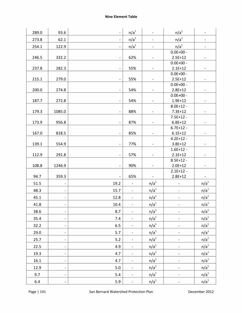
Nine Element Table
Page | 141 San Bernard Watershed Protection Plan December 2012
289.0 93.6 - n/a1 - n/a1 -
273.8 62.1 - n/a1 - n/a1 -
254.1 122.9 - n/a1 - n/a1 -
246.5 332.2 - 62% - 0.0E+00 - 2.5E+12 -
237.8 282.3 - 55% - 0.0E+00 - 2.1E+12 -
215.1 279.0 - 55% - 0.0E+00 - 2.5E+12 -
200.0 274.8 - 54% - 0.0E+00 - 2.8E+12 -
187.7 272.8 - 54% - 0.0E+00 - 1.9E+12 -
179.3 1085.0 - 88% - 8.0E+12 - 7.3E+12 -
173.9 956.8 - 87% - 7.5E+12 - 6.8E+12 -
167.0 818.5 - 85% - 6.7E+12 - 6.1E+12 -
139.1 554.9 - 77% - 4.2E+12 - 3.8E+12 -
112.9 291.8 - 57% - 1.6E+12 - 2.1E+12 -
108.8 1246.9 - 90% - 8.5E+12 - 2.0E+12 -
94.7 359.3 - 65% - 2.1E+12 - 2.8E+12 -
51.5 - 19.2 - n/a1 - n/a1
48.3 - 15.7 - n/a1 - n/a1
45.1 - 12.8 - n/a1 - n/a1
41.8 - 10.4 - n/a1 - n/a1
38.6 - 8.7 - n/a1 - n/a1
35.4 - 7.4 - n/a1 - n/a1
32.2 - 6.5 - n/a1 - n/a1
29.0 - 5.7 - n/a1 - n/a1
25.7 - 5.2 - n/a1 - n/a1
22.5 - 4.9 - n/a1 - n/a1
19.3 - 4.7 - n/a1 - n/a1
16.1 - 4.7 - n/a1 - n/a1
12.9 - 5.0 - n/a1 - n/a1
9.7 - 5.4 - n/a1 - n/a1
6.4 - 5.9 - n/a1 - n/a1

Nine Element Table
Page | 142 San Bernard Watershed Protection Plan December 2012
3.2 - 13.0 - n/a1 - n/a1 *Sub-watersheds not showing a load reduction needed are at or below the standard.
FIGURE A.17 SOURCE LOADING BOX PLOT
1.E+00
1.E+01
1.E+02
1.E+03
1.E+04
1.E+05
1.E+06
1.E+07
1.E+08
1.E+09
1.E+10
1.E+11
1.E+12
Wildlife Septic Livestock Point Source
E. c
oli
(MP
N/d
L)

Nine Element Table
Page | 143 San Bernard Watershed Protection Plan December 2012
Causes and Sources of Bacteria
Implementation Activities
Estimated Load Reduction
Technical and Financial Needs
Education Component
Schedule for Implementation
Interim, Measureable Milestones
Indicators to measure progress
Monitoring Component
Responsible Entity
OSSFs
33% reduction needed to meet WQ standadrs
Identification and repair of malfunctioning systems
90% SEP funds, 319 grant funding, AgriLife extension Repair: $5,000 Replacement: $10,000
Homeowner workshops, Authorized agent training
Ongoing identification and repair of failing systems
Number of systems repaired and inspected on an annual basis
ecoli reductions, determining locations of systems
reports from Authorized Agents, tracking of systems on website
Authorized Agents to inspect, homeowners to repair and replace, H-GAC to inventory and map
Wildlife
40% reduction needed to meet WQ standards
Landowner workshops to facilitate identification of damage from and capture of feral hogs
<5% Technical: TexasAgrilife extension, SEP funds Workshops: $8,000
Landowner workshops
Ongoing and expanding programs
Number of hogs managed each year, number of pork choppers flying area
ecoli reductions, number of hogs reported killed
reports on damage
Texas Parks and Wildlife and Texas AgriLife extension
Livestock
18% reduction needed to meet WQ standards
WQMPs that include fencing, alternate water sources and/or prescribed grazing
75% Technical: TSSWCB Cost: $10,000 - $15,000 each
Advertisement of WQMPs
Ongoing Number of plans implemented each year
ecoli reductions, number of plans implementing livestock management measures
reports of plans
TSSWCB, landowners
Agriculture
WQMPs that include measures to reduce soil and sediment loss to area waterways
10% Technical: TSSWCB Cost: $10,000 - $15,000 each
Advertisement of WQMPs
Ongoing Number of plans implemented each year
ecoli reductions, number of plans implementing
reports TSSWCB, landowners

Nine Element Table
Page | 144 San Bernard Watershed Protection Plan December 2012
agriculture management measures
WWTFs
10% reduction needed to meet WQ standards
Monitoring of WWTF effluent to determine bacteria levels
5% Technical: TCEQ, TSSWCB grant funding additional monitoring Testing: $25/month/facility
Facility operator education
Implementation of bacteria testing with permit renewal
number of facilities meeting standards and within limits
reductions in base levels based on actual bacteria counts
reports to TCEQ of bacteria levels, monitoring levels
Facility operators/Cities/MUDs, TCEQ
Land Management
Model ordinances 5% Technical: H-GAC landowner education
Ongoing Number of ordinances or pollution prevention plans created
ecoli reductions in areas with ordinances
reports from cities
Cities
Conservation easements/Filter Strips/Grassed Waterways
>10% Technical: Counties, SEP funds Cost: Depends on size & location
Landowner education
Ongoing number of conservation easements/acres protected
ecoli reductions in areas with easements
reports of conservation easement contracts
Landowners, nonprofits
Clean up of illegal dumping
1% Technical: Counties, solid waste grants Cost: $40,000
Landowner education
ongoing number of sites cleaned up/tons of trash collected
reduction in number of items dumped in waterways
reports from counties about cleanups,
Counties