S ILV FENNICA - Metla · In the common methods of forest mensuration, ... Circle Area Formula ... 9 Summary and Conclusions

SILVA FENNICA

The Finnish Society of Forest ScienceThe Finnish Forest Research Institute

Vol. 46(5B), 2012

Minna Pulkkinen

On Non-Circularity of Tree Stem Cross-Sections: Effect of Diameter Selection on Cross-Section Area Estimation, Bitterlich Sampling and Stem Volume Estimation in Scots Pine

Cover photo by Metla/Erkki Oksanen

Abstract

Pulkkinen, M. 2012. On non-circularity of tree stem cross-sections: Effect of diameter selection on cross-section area estimation, Bitterlich sampling and stem volume estima-tion in Scots pine. Silva Fennica 46(5B): 747–986.

In the common methods of forest mensuration, including stem volume models and Bit-terlich sampling, stem cross-sections are assumed to be circular. In nature this assumption is never exactly fulfilled. Errors due to non-circularity have been presumed to be small and unimportant but studied little: theoretical and empirical studies exist on cross-section area estimation, but errors in stem volume estimation have not been investigated at all, and errors in Bitterlich sampling are theoretically known only for stand basal area estimation. In the theoretical part of this study, we developed methods for quantifying the systematic and sampling errors that 22 common ways of selecting diameter within non-circular cross-sections induce (i) in area estimates by the circle area formula, (ii) in stand total estimates by Bitterlich sampling, and (iii) in stem volume estimates by a volume equation, by a cubic-spline-interpolated stem curve, and by a generalised volume estimator. In the empirical part, based on the digital images of 709 discs taken at 6–10 heights in 81 Scots pine stems from different parts of Finland, we investigated the varia-tion in cross-section shape, and demonstrated the magnitude of the errors presented in the theoretical part. We found that non-circularity causes systematic overestimation of area and volume, and inflicts potentially systematic error on stand total estimates by Bitterlich sampling. In our data these effects were small, but the finding is not generalisable due the skewed size distribution and poor geographical representativeness of the data. We recommend using diameter derived from girth for both tree and stand level estimation, as it involves no sampling error and produces clearly the most stable systematic errors.

Keywords forest mensuration, cross-section, non-circularity, basal area, stem volume, Bitterlich sampling, Scots pineE-mail [email protected] 21 September 2012 Accepted 12 December 2012Available at http://www.metla.fi/silvafennica/full/sf46/sf465747.pdf

Silva Fennica 46(5B), 2012 research articles

749

Pulkkinen On Non-Circularity of Tree Stem Cross-Sections: Effect of Diameter Selection …

ContentsAcknowledgements ...................................................................................................751List of Symbols .........................................................................................................7531 Introduction ........................................................................................................757Theory2 Geometrical and Statistical Concepts ..............................................................7613 Estimation of Cross-Section Area .....................................................................769

3.1 Foundations: Source of Randomness and Measures of Estimator Performance .................................................................................769

3.2 Effect of Non-Convexity ..............................................................................7703.3 Estimators Based on Diameters and Circle Area Formula ...........................770

3.3.1 Girth Diameter: Mean Diameter Derived from Convex Perimeter ....7713.3.2 Random Diameters with Uniform Direction Distribution ..................7723.3.3 Minimum and Maximum Diameters ..................................................780

3.4 Estimators Based on Radii ...........................................................................7814 Bitterlich Sampling ............................................................................................783

4.1 Estimation of Stand Totals............................................................................7844.1.1 Principle under Assumption of Circular Cross-Sections ....................7854.1.2 Effect of Non-Circularity of Cross-Sections ......................................7874.1.3 Special Case: Relative Basal Area .....................................................795

4.2 Bitterlich Diameters: Diameters Measured Parallel or Perpendicular to Plot Radius Direction ...................................................................................7994.2.1 Direction Distributions of Bitterlich Diameters .................................8004.2.2 Estimation of Cross-Section Area by Bitterlich Diameters and

Circle Area Formula ...........................................................................8035 Estimation of Stem Volume ...............................................................................808

5.1 Practical Volume Estimator: Laasasenaho Volume Equation .......................8085.2 General Volume Estimator: Definite Integral of Cross-Section Area

Estimation Function ..................................................................................... 8115.3 Volume Estimator Based on Non-Parametric Stem Curve: Definite

Integral of Interpolating Cubic Splines ........................................................814Practice6 Material ...............................................................................................................8197 Methods ...............................................................................................................826

7.1 Cross-Section Shape .....................................................................................8267.1.1 Shape of Convex Closure ...................................................................8277.1.2 Non-Convexity ...................................................................................8297.1.3 True Shape ..........................................................................................830

7.2 Estimation of Cross-Section Area ................................................................8327.3 Estimation of Stem Volume ..........................................................................836

7.3.1 True Volume .......................................................................................8387.3.2 Laasasenaho Volume Equation ...........................................................8397.3.3 Cubic-Spline-Interpolated Stem Curve ..............................................8427.3.4 General Volume Estimator .................................................................844

7.4 Estimation of Stand Totals in Bitterlich Sampling .......................................846

750


8 Results with Discussion .....................................................................................8498.1 Caveats on Data ............................................................................................8498.2 Cross-Section Shape .....................................................................................851

8.2.1 Shape of Convex Closure ...................................................................8518.2.2 Non-Convexity ...................................................................................8608.2.3 True Shape ..........................................................................................863

8.3 Estimation of Cross-Section Area ................................................................8688.3.1 Reference Estimator Based on Girth Diameter ..................................8688.3.2 Comparison of Area Estimators .........................................................872

8.4 Estimation of Stem Volume ..........................................................................8888.4.1 Laasasenaho Volume Equation ...........................................................8928.4.2 Cubic-Spline-Interpolated Stem Curve ..............................................9018.4.3 General Volume Estimator .................................................................912

8.5 Estimation of Stand Totals in Bitterlich Sampling .......................................918Synthesis9 Summary and Conclusions ...............................................................................926References ................................................................................................................935Appendices ...............................................................................................................940

Appendix A Support Function of Closed Convex Set or Curve in Plane ..........940Appendix B Horvitz-Thompson Theorem .........................................................944Appendix C Expressing Boundary Co-ordinates, Radii and Total Area

of Inclusion Region of Tree in Bitterlich Sampling in Terms of Support Function of Breast Height Cross-Section ................................................................................947

Appendix D Expressing Probability Distribution of Bitterlich Diameter Direction in Terms of Support Function of Breast Height Cross-Section of Tree ........................................................951

Appendix E Within-Tree Expectations of Volume Predictions by Laasasenaho Volume Equation with Diameter Selection Methods 1–5, 1ξ–5ξ, 1ξ90, 4ξ90 and 5ξ90 ...................................956

Appendix F Within-Tree Variances of Volume Predictions by Laasasenaho Volume Equation with Diameter Selection Methods 1–5, 1ξ–5ξ, 1ξ90, 4ξ90 and 5ξ90 ..........................................................961

Appendix G Computation of Diameters, Breadths and Radii from Vector Image of Cross-Section .................................................................971

Appendix H Computation of Contour Co-ordinates, Sector Areas and Total Area of Inclusion Region in Bitterlich Sampling from Vector Image of Cross-Section .............................................976

Appendix I Computation of Scale in Vector Image of Cross-Section ..............980Appendix K Examples of Association between Some Shape Indices

and Actual Shapes of Cross-Sections ............................................984

751


AcknowledgementsMany people gave invaluable help in this study. The topic was suggested to me by Juha Lappi, who first became a supervisor and then a friend. I wish to thank him warmly and sincerely for his pertinent advice and lucid comments, particularly in the earlier phase of the work, for his alert action in the final publication phase of the work, and for the many profound discussions that we have had throughout the years.

The work began as a MSc project at the then Faculty of Forestry of the University of Joensuu (nowadays the School of Forest Sciences of the University of Eastern Finland). The disc data were generously provided by the VAPU project of the Finnish Forest Research Institute led by Kari T. Korhonen at the Joensuu Research Station. The discs were photo-graphed by Matti Hälinen, using the rack system constructed by the staff in the Imaging Centre of the University; these staff also printed the photographs. With the vectorisation of the raster images of the scanned photographs, Janne Soimasuo and Ari Turkia lent a cru-cially helping hand. I am indebted to all these persons for their indispensable contribution.

All along the way, Bertil Matérn inspired the work with his excellent early (1956) paper. He was also kind enough to elucidate, in an exchange of letters, the issues in the paper that I was not able to fathom out myself. Further, he generously placed at my disposal some older literature that is hard to get hold of. I wish I could have completed the work before his demise, so that he could have appraised the extension of his original ideas, particularly those about the effect of non-circularity on Bitterlich sampling.

The ideas on Bitterlich sampling started to germinate during my working in the spatial statistics group led by Antti Penttinen at the Department of Statistics of the University of Jyväskylä, and during my half-year visit to the spatial statistics group at the Department of Mathematical Sciences of Aalborg University. I am grateful to these two statistics com-munities for sowing the seeds of the ideas in my mind, as well as for setting good examples of rigorous statistical thinking and presentation.

I carried out almost all the computation work after the MSc thesis, as well as a consider-able part of writing, at the Vantaa Research Centre of the Finnish Forest Research Institute. The group of forest yield and growth study, and later also the group of forest technology, became my hearth and home there. My thanks are due to the researchers and other staff for their approving and encouraging attitude, and to the Institute for very good working facilities. Particularly, I am indebted to Carl-Gustaf Snellman for his assistance in com-putational problems, and to Jari Hynynen for arranging additional funding after the grant awarded for the work ran out. I also gratefully acknowledge Sointu Virkkala for drawing Figure 22. At that time, Timothy Gregoire was kind to send me the copies of some highly relevant works, especially those by G. R. Grosenbaugh that would have been difficult to obtain otherwise, for which I express my gratitude.

Outside the research institutions, Harri Hypén played an important role. I am especially obliged to him for one significant brainstorm, during a car drive to Eastern Finland, in which we sketched the algorithm for computing the inclusion regions of trees in Bitterlich sampling from the vector images of the cross-section contours. I also gratefully acknowledge him for drawing the original version of Figure 25.

I resumed writing, after a considerable break, while working at the Departments of Forest Ecology and Forest Resource Management (nowadays merged into one, the Department of Forest Sciences) of the University of Helsinki. I wish to give my heartfelt thanks to Annikki Mäkelä and Pauline Stenberg, my superiors, for their encouragement and sup-port, which they gave also in the concrete form of arranging funding. My thanks are also due to the colleagues in the forest ecology modelling group, from whom I learnt much of doing research work, particularly the necessity of always asking what one’s results really

752


mean and imply, which then benefitted the writing of the thesis. Pertti Hari deserves spe-cial thanks for initiating and persisting with regular mentoring discussions, as a result of which the focus of the work was changed from empirical to theoretical findings. Finally, I wish to give recognition to all the people at the Department for making it such a lively and versatile community, to which it was a pleasure to belong, also outside the working hours.

In the finalisation phase, Christophe Godin’s help and support was indispensable. I am much obliged to him for the discussions that helped shape the introductory and summary chapters, as well as for the pivotal technical solutions for converting the manuscript into the format required by the publisher.

Juha Heikkinen and Göran Ståhl, the official pre-examiners, gave a substantial amount of their time for reviewing the thesis. I wish to thank them sincerely for their work. Matti Maltamo, the professor of forest mensuration formally responsible for the defence process, deserves thanks for his upholding attitude and prompt aid in all the technicalities related to the process.

Numerous institutions funded the study: the COMAS Graduate School of the University of Jyväskylä, the Academy of Finland, the Faculty of Forestry of the University of Joensuu / the School of Forest Sciences of the University of Eastern Finland, and the Foundation for Research of Natural Resources in Finland (grants number 1552/99, 1578/00, 1603/01) are hereby gratefully acknowledged.

Throughout the years, my near and dear, close and far, have tried to make me see, under-stand and remember the beauty of life, in its myriad aspects. I wish to give them my deepest thanks for this. As Mephistopheles puts it in his well-known words in J. W. von Goethe’s play Faust: “Grau, theurer Freund, ist alle Theorie, und grün des Lebens goldner Baum [My friend, all theory is grey, and green the golden tree of life].”

753


List of SymbolsCross-SectionA area of a cross-sectionAC area of the convex closure of a cross-sectionÂj estimator of cross-section area based on the circle area formula and

diameter selection method jÂGj generalisation of estimator Âj for n similarly selected diameters(AC–A)/AC relative convex deficit of a cross-section(Â0–AC)/AC relative isoperimetric deficit of a cross-sectionB(θ) breadth of a cross-section in direction θ, with respect to the centre of

gravity; B:[0, π)→(0, ∞)BC(θ) breadth of the convex closure of a cross-section in direction θ, with

respect to the centre of gravity; BC:[0, π)→(0, ∞)be/ae girth-area ellipse ratio of a cross-section; axis ratio of the ellipse that has

the same perimeter and area as the convex closure of a cross-sectionC girth of a cross-section; perimeter of the convex closure of a cross-sectionCp perimeter of a cross-sectionCVD coefficient of variation of diameter in a cross-section; CVD=σD/μDD(θ) diameter of a cross-section in direction θ; D:[0, π)→(0, ∞)DA true area diameter of a cross-section; diameter that produces the area of

a cross-section when substituted in the circle area formula; DA=2[A/π]1/2

DAc convex area diameter of a cross-section; diameter that produces the area of the convex closure of a cross-section when substituted in the circle area formula; DAc=2[AC/π]1/2

Dmax maximum diameter of a cross-sectionDmin minimum diameter of a cross-sectionFξ(ξ; α) cumulative distribution function of diameter direction ξ parallel to plot

radius in Bitterlich sampling with viewing angle αfξ(ξ; α) probability density function of diameter direction ξ parallel to plot radius

in Bitterlich sampling with viewing angle αp(θ) support function of the convex closure of a cross-section; p:[0, 2π)→(0, ∞)R(θ) radius of a cross-section in direction θ from the centre of gravity;

R:[0, 2π)→(0, ∞)RC(θ) radius of the convex closure of a cross-section in direction θ from the

centre of gravity; RC:[0, 2π)→(0, ∞)Rmax maximum radius of a cross-sectionRq quadratic mean of the observed radii in a cross-sectionR landmark configuration of a cross-section; collection of the observed

radii in a cross-section; R=(R(j·1°))j=0, 1, ..., 359R* centred pre-shape of a landmark configuration of a cross-section;

R*=(R*(j·1°))j=0, 1, ..., 359 =(R(j·1°)/Rq)j=0, 1, ..., 359

θ general symbol of direction; diameter direction with uniform distribution in [0, π)

θDmax direction of DmaxθDmin direction of DminθRmax direction of Rmaxτ plot radius direction in Bitterlich samplingξ diameter direction parallel to plot radius in Bitterlich sampling; ξ~Fξ(ξ; α)

with viewing angle α

754


μD girth diameter of a cross-section; within-cross-section expectation of diameter over the uniform direction distribution in [0, π); μD=C/π

μD(ξ) mean Bitterlich diameter, parallel to plot radius, in a cross-section; within-cross-section expectation of diameter over the distribution of the diameter direction ξ parallel to plot radius in Bitterlich sampling

μD(ξ+π/2) mean Bitterlich diameter, perpendicular to plot radius, in a cross-section; within-cross-section expectation of diameter over the distribution of the diameter direction ξ+π/2 perpendicular to plot radius in Bitterlich sampling

σD2 diameter variance in a cross-section; within-cross-section variance of diameter over the uniform direction distribution in [0, π)

σD(ξ)2 variance of Bitterlich diameters, parallel to plot radius, in a cross-section; within-cross-section variance of diameter over the distribution of the diameter direction ξ parallel to plot radius in Bitterlich sampling

σD(ξ+π/2)2 variance of Bitterlich diameters, perpendicular to plot radius, in a cross-section; within-cross-section variance of diameter over the distribution of the diameter direction ξ+π/2 perpendicular to plot radius in Bitterlich sampling

γD(φ) within-cross-section covariance of the diameters intersecting at angle φ over the uniform direction distribution in [0, π); diameter autocovariance function in a cross-section; γD:[0, π/2)→[0, ∞)

ρD(φ) within-cross-section correlation of the diameters intersecting at angle φ over the uniform direction distribution in [0, π); diameter autocorrelation function in a cross-section; ρD:[0, π/2]→[–1, 1]

ρD(π/2) within-cross-section correlation of perpendicular diameters over the uniform direction distribution in [0, π)

ρD(ξ)(π/2) within-cross-section correlation of the diameters parallel and perpen-dicular to plot radius in Bitterlich sampling

StemA(h) area of the cross-section of a stem at height h; cross-section area function;

A:[0, H]→[0, ∞)Âj(h) estimator of the area of the cross-section of a stem at height h based on

the circle area formula and diameter selection method j; area estimation function; Âj:[0, H]→[0, ∞)

D(θ, h) diameter in direction θ at height h, θ∈[0, π)Dj(h) diameter selected with method j at height h DA(h) true area diameter DA at height h; true stem curve; DA:[0, H]→[0, ∞)DAc(h) convex area diameter DAc at height hDj vector of diameters selected with method j at the observation heights H

in a stemDA vector of true area diameters at the observation heights H in a stemDAc vector of convex area diameters at the observation heights H in a stemH length of a stem; height of a tree determined from the ground levelH vector of the observation heights in a stemV true volume of a stemV estimated true volume of a stem; V=VSVC convex volume of a stem (approximately the volume of the convex hull

of a stem)VC estimated convex volume of a stem; VC=VCS

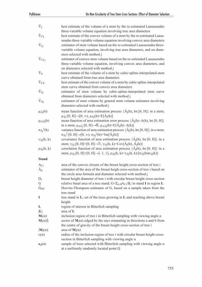
755


VL best estimate of the volume of a stem by the re-estimated Laasasenaho three-variable volume equation involving true area diameters

VCL best estimate of the convex volume of a stem by the re-estimated Laasa-senaho three-variable volume equation involving convex area diameters

VLj estimator of stem volume based on the re-estimated Laasasenaho three-variable volume equation, involving true area diameters, and on diam-eters selected with method j

VCLj estimator of convex stem volume based on the re-estimated Laasasenaho three-variable volume equation, involving convex area diameters, and on diameters selected with method j

VS best estimate of the volume of a stem by cubic-spline-interpolated stem curve obtained from true area diameters

VCS best estimate of the convex volume of a stem by cubic-spline-interpolated stem curve obtained from convex area diameters

VSj estimator of stem volume by cubic-spline-interpolated stem curve obtained from diameters selected with method j

VGj estimator of stem volume by general stem volume estimator involving diameters selected with method j

μÂj(h) mean function of area estimation process {Âj(h), h∈[0, H]} in a stem; μÂj:[0, H]→[0, ∞), μÂj(h)=E[Âj(h)]

μΔÂj(h) mean function of area estimation error process {Âj(h)–A(h), h∈[0, H]} in a stem; μΔÂj:[0, H]→R, μΔÂj(h)=E[Âj(h)–A(h)]

σÂj2(h) variance function of area estimation process {Âj(h), h∈[0, H]} in a stem; σÂj2:[0, H]→[0, ∞), σÂj2(h)=Var[Âj(h)]

γÂj(h, k) covariance function of area estimation process {Âj(h), h∈[0, H]} in a stem; γÂj:[0, H]×[0, H]→R, γÂj(h, k)=Cov[Âj(h), Âj(k)]

ρÂj(h, k) correlation function of area estimation process {Âj(h), h∈[0, H]} in a stem; ρÂj:[0, H]×[0, H]→[–1, 1], ρÂj(h, k)=γÂj(h, k)/[σÂj(h)σÂj(k)]

StandACi area of the convex closure of the breast height cross-section of tree iÂji estimator of the area of the breast heigh cross-section of tree i based on

the circle area formula and diameter selected with method jDi breast height diameter of tree i with circular breast height cross-sectionG relative basal area of a tree stand; G=Σi∈IACi/|L| in stand I in region L ĜHT Horvitz-Thompson estimator of G, based on a sample taken from the

tree stand I tree stand in L; set of the trees growing in L and reaching above breast

heightL region of interest in Bitterlich sampling|L| area of LMi(α) inclusion region of tree i in Bitterlich sampling with viewing angle αMi(α)ba sector of Mi(α) edged by the rays emanating in directions a and b from

the centre of gravity of the breast height cross-section of tree i|Mi(α)| area of Mi(α)ri(α) radius of the inclusion region of tree i with circular breast height cross-

section in Bitterlich sampling with viewing angle αsQ(α) sample of trees selected with Bitterlich sampling with viewing angle α

at a uniformly randomly located point Q

756


Y total amount of a characteristic of interest in a tree stand; Y=Σi∈IYi in stand I in region L

ŶHT Horvitz-Thompson estimator of Y, based on a sample taken from the tree stand

α viewing angle in Bitterlich sampling, relascope angleκi(α) basal area factor of tree i in Bitterlich sampling with viewing angle α;

κi:(0, π)→(0, 1), κi(α)=ACi/|Mi(α)|πi(α) inclusion probability of tree i growing in L in Bitterlich sampling with

viewing angle α; πi(α)=|Mi(α)|/|L|GeneralPr{A} probability of event AS3(a; A, B) interpolating cubic spline based on the vector B of values observed at

the vector A of one-dimensional locationsδi(A) random indicator variable; δi(A)=1, if i∈A, and δi(A)=0, if i∉ADiameter Selection Methods within Cross-Section0 girth diameter; mean diameter μD=C/π of over the uniform direction

distribution in [0, π)1 “random” diameter; diameter taken in a uniformly distributed direction

in [0, π)2 arithmetic mean of the diameter in 1 and the diameter perpendicular to

it3 geometric mean of the diameters in 24 arithmetic mean of two “random diameters”; arithmetic mean of two

diameters taken independently in uniformly distributed directions in [0, π)

5 geometric mean of the diameters in 46 arithmetic mean of the minimum diameter and the maximum diameter7 geometric mean of the diameters in 68 arithmetic mean of the minimum diameter and the diameter perpendicular

to it9 geometric mean of the diameters in 810 arithmetic mean of the maximum diameter and the diameter perpendicular

to it 11 geometric mean of the diameters in 101ξ diameter taken parallel to plot radius in Bitterlich sampling2ξ arithmetic mean of the diameters in taken parallel and perpendicular to

plot radius in Bitterlich sampling3ξ geometric mean of the diameters in 2ξ4ξ arithmetic mean of the diameter taken parallel to plot radius in Bitterlich

sampling and a diameter taken independently in a uniformly distributed direction in [0, π)

5ξ geometric mean of the diameters in 4ξ1ξ90 diameter taken perpendicular to plot radius in Bitterlich sampling4ξ90 arithmetic mean of the diameter taken perpendicular to plot radius in

Bitterlich sampling and a diameter taken independently in a uniformly distributed direction in [0, π)

5ξ90 geometric mean of the diameters in 4ξ90min minimum diametermax maximum diameter

757


1 IntroductionIn the common methods of forest mensuration, the cross-sections of tree stems are assumed to be circular: The area of a stem cross-section is usually estimated with the circle area formula. The volume of a stem is typically estimated as the solid of revolution of a stem curve, or with a volume equation constructed with a combination of circle-base geometric solids (cones, paraboloids, neiloids) as the starting point. Trees to be measured in forest inventories are often selected with Bitterlich sampling (relascope sampling), where the inclusion probabilities, required in the estimator of the stand total of any characteristic of interest, are estimated by assuming that the breast height cross-sections of the selected trees are circular. The basal area of a stand is estimated either as the sum of the treewise estimates of cross-section area given by the circle area formula, or, as is most often the case in practi-cal forestry, by multiplying the number of trees selected in Bitterlich sampling with the so called basal area factor; the latter is a special case of the stand total estimation in Bitterlich sampling and thus assumes circularity on the breast height cross-sections of the trees.

In nature, however, the cross-sections of tree stems are hardly ever exactly circular. Non-circularity occurs due to defects and deformations inflicted by pathogens or mechanical damages, but also without them, in entirely healthy and undamaged trees. Asymmetric growing space affecting the access of a tree to light has been suggested to be one potential cause of non-circularity: with uneven spatial distribution of light, the crown would develop asymmetrically, and the stem should then compensate the resulting mass imbalance by increased wood formation in the direction of the torsional moment. Observations have been reported both for (e.g. Isomäki 1986, Robertson 1991) and against (e.g. Bucht 1981, Bouillet and Houllier 1994) this idea. Wind is another factor proposed to induce non-circularity (Banks 1973, Grace 1977). The mechanism would essentially be similar to the one suggested above: winds blowing continuously from the same direction would cause a torsional moment, which the stem should then counteract by forming more wood in the direction of the wind. Observations supporting this idea have been reported, for example, by Müller (1958a) and Robertson (1986, 1990, 1991). Through the same mechanism, growing in a steep slope or in a leaning position could also result in non-circular stems (Pawsey 1966, Loetsch et al. 1973). Regular heavy snow loads, in turn, could encourage trees to develop straight stems with circular cross-sections to resist the bending forces of the load (Professor emeritus Pertti Hari, personal communication). In general, eccentric radial growth has often been found to be associated with reaction wood formation (e.g. Burdon 1975, Harris 1977, Robertson 1991). The factors listed above could explain the age-related variation in non-circularity: old trees tend to have more irregular cross-sections than young ones, simply because they have been exposed to inflicting growing conditions for a longer time. However, even if growing in similar conditions, some species appear to be more non-circular than others: according to Kärkkäinen (2003), broad-leaved species in Finland are in general more non-circular than coniferous ones; Loetsch et al. (1973), in turn, mention Tectona grandis, Carpinus betulus and Robinia pseudacacia as the species with very irregular cross-sections.

Following from the circularity assumption, the key characteristic of a stem cross-section is its diameter. Yet in a non-circular cross-section there is no single diameter value but diam-eter varies with direction. In practice, diameter is typically measured with a caliper, which gives the distance between two parallel tangents (that are perpendicular to the direction in which the diameter is being measured), or with a girth tape, by dividing the perimeter measurement by π, which gives the mean of the calipered diameter over all directions (as we will see in Chapter 2). It is important to differentiate between diameter variation due to non-circular shape and diameter variation caused by measurement errors (arising from faulty

758


handling of instruments, adverse measurement conditions, psychological factors etc.); in literature this distinction has not always been made, but genuine measurement errors have erroneously been ascribed to non-circularity (Matérn 1990).

Variation in diameter within a cross-section of a tree causes variation in the output of such a cross-section area or volume estimator where the diameter is used as an input variable: the estimate of area or volume depends on the selection of diameter. This selection involves the choice of the measurement direction, the number of diameters to be measured and the type of mean (geometric, arithmetic, quadratic) to be applied to the measured diameters. Volume models often involve diameters at more than one height in the stem; the more heights are involved the more complex variation non-circularity potentially induces in the volume estimates. The within-tree variation in estimator output can be characterised by bias and variance. Bias is a measure of the systematic error due to non-circularity: it is the deviation of the mean of all possible estimates, obtained with all possible outcomes of the diameter selection, from the true value, or in other words, the mean error expected over all possible outcomes of the diameter selection. Variance of all possible estimates around their mean, in turn, quantifies the sampling error related to non-circularity; from it we can derive the likely range of the error in the estimate associated with one outcome of the diameter selection.

In Bitterlich sampling, variation in diameter within the breast height cross-section causes variation in the estimate of the inclusion probability of a tree, since the estimator of the probability, based on the circularity assumption, involves the breast height diameter as its input variable. In addition (as we will see in Chapter 4; not shown before), non-circularity inflicts another separable error component in the inclusion probability estimate, dependent only of the cross-section shape and independent of diameter selection. The combination of these errors then decides how the tree contributes, due to its non-circularity, to the bias of the stand total estimator of any characteristic of interest.

In his path-breaking study, Matérn (1956) derived, without postulating anything about the shape of a cross-section, the bias and the approximative variance for the area esti-mators based on the circle area formula and some common diameter selection methods (diameter derived from perimeter, diameter calipered in a random direction, mean of this diameter and its perpendicular, or mean of two diameters calipered in random directions). On the basis of the bias formulae, he could show that these area estimators systematically overestimate true cross-section area. Furthermore, he developed theory on the effect of non-circularity on basal area estimation with Bitterlich sampling and was able to establish that the overestimating bias induced by non-circularity is practically (with the commonly used small viewing angles) the same as we would get by calipering every stem in one randomly chosen direction. In a later work (1990), he then applied this theory in data that consisted of contour drawings made on over one hundred discs sawn on a about forty Scots pine and Norway spruce stems. Besides Matérn’s work, no other theoretical developments concerning the effect of within-cross-section diameter variation on area estimation are to be found in literature. Likewise, the effect of non-circularity on stem volume estimation or on estimation of other stand totals than basal area in Bitterlich sampling appear hitherto theoretically unexplored.

Many empirical studies addressing non-circularity have focused on the shape of cross-sections, investigating with simple shape indices to what extent cross-sections deviate from a circle and how this deviation is related to position of the cross-section in the stem, tree species, silvicultural treatments, growing conditions etc. (e.g. Renvall 1923, Solbraa 1939, Williamson 1975, Kellogg and Barber 1981, Okstad 1983, Mäkinen 1998). Another large set of empirical studies have concerned cross-section area estimation with the circle area formula and different diameter selection methods, reporting differences in area estimates between the diameter selection methods and, more recently with the emergence of less

759


laborious area measurement methods, also the errors with respect to true area (e.g. Kennel 1959, Chacko 1961, Kärkkäinen 1975a, Biging and Wensel 1988, Gregoire et al. 1990). In many of these studies, in particular earlier ones, data consist of field measurements with a caliper or a girth tape and are thus very likely to contain measurement errors. A clearly distinct branch of studies, making use of ample data of cross-section radii provided by scanners employed in sawmills, have tested different models of cross-section shape with the aim of adapting sawing patterns to maximise the sawing yield (e.g. Skatter and Høibø 1998, Saint-André and Leban 2000). Practically no empirical studies seem to exist concerning the effect of within-cross-section diameter variation on volume estimation nor concerning the effect of non-circularity on Bitterlich sampling.

Nonetheless, the effects of non-circularity are worth investigating, even though other sources of error (sampling errors, measurement errors, model misspecification errors, estimation errors in model parameters, model residual errors) probably induce much more uncertainty in the results of forest inventories: on the basis of Matérn’s theoretical results, it is realistic to anticipate that non-circularity might inflict systematic errors also in volume estimates and stand total estimates by Bitterlich sampling, and that these, although presum-ably small in magnitude, can then cumulate into considerable errors in large area inven-tories. Further, in research purposes where one often strives for eliminating confounding factors, taking non-circularity effect into account may clarify and consolidate the results of analyses; particularly, when estimating growth with the difference between diameters, cross-section areas or stem volumes at two time points, the potentially asymmetric growth in non-circular cross-sections need be heeded.

This study concerns the effects of non-circularity on (i) cross-section area estimation with the circle area formula, (ii) stand total estimation in Bitterlich sampling with the circularity assumption, and (iii) stem volume estimation by a standard three-variable volume equation, by a non-parametric stem curve often applied in research purposes, and by a theoretical general volume estimator based on a cross-section area estimation function. The estimators considered are commonly used for standing trees or felled sample trees and involve dimen-sions of stems that can be measured from outside with the usual measurement equipment (calipered diameters, perimeters given by a tape, height obtained with a hypsometer or a tape). The diameter selection methods included in the examination are such that they exist in literature and are used, or could in principle be used, in practice. The first aim of the study was to develop further the existing theory: to derive the missing statistical properties of the area estimators under within-cross-section diameter variation, to devise methods for estimating similar statistical properties for the volume estimators, and to unravel theoreti-cally how non-circularity affects Bitterlich sampling, without postulating anything about cross-section shape. The second aim of the study was to investigate with reasonable data how cross-section shape varies in Scots pine and of what magnitude the above-mentioned theoretically established effects of non-circularity can be in practice.

In the theoretical part of the work, we (i) derived the within-cross-section bias, approxi-mative variance and true variance for the area estimators based on the circle area formula and five common diameter selection methods (involving diameters calipered in randomly chosen directions and their perpendiculars; methods already addressed by Matérn), as well as their generalisations up to n diameters, (ii) described how non-circularity of breast height cross-sections influences inclusion probabilities of trees and hence stand total estimation in Bitterlich sampling, (iii) derived the non-uniform direction distributions for the diameters measured parallel or perpendicular to plot radius in Bitterlich sampling, and presented the within-cross-section bias, approximative variance and true variance for the area estima-tors based on the circle area formula and eight diameter selection methods involving these diameters, and (iv) presented methods for estimating the within-tree bias and variance of

760


the three types of volume estimators (volume equation, non-parametric stem curve, theo-retical general volume estimator based on a cross-section area estimation function) with the diameter selection methods considered in (i) and (iii).

The empirical part of the work relied on the data of 709 discs taken at 6–10 heights in 81 healthy Scots pine stems in different parts of Finland; to eliminate measurement errors, the characteristics of the cross-sections were computed from digital images. With these data, we (i) investigated the variation in cross-section shape in different parts of the stems by means of some scalar and functional indices, (ii) estimated the within-cross-section biases and variances of the area estimators based on the circle area formula and 22 diameter selection methods (including those considered in the theoretical part), (iii) estimated the within-tree biases and variances of the three types of volume estimators with the same 22 diameter selection methods, and (iv) estimated, still with the same 22 diameter selection methods, the tree-specific errors caused by non-circularity in the inclusion probabilities in Bitterlich sampling, imparting the contribution of each tree in the bias of a stand total estimate. Owing to some defects in the data (non-probabilistic sampling of trees with uneven spatial distribution over Finland, skewed size distribution with small trees highly over-represented, debarking of discs before imaging), the empirical results cannot be gener-alised to any defined population (such as the Scots pine trees in Finland) or do not compare with the usual characteristics (that include bark) but should rather be taken as illustrations.

As a final remark, non-circularity was here studied as a static geometric phenomenon: the biological processes forming cross-section shape and the factors influencing these pro-cesses (site conditions, competition, management history of the stand etc.) were beyond the scope of this study.

761


2 Geometrical and Statistical ConceptsIn this chapter, we introduce the notions of convex closure and support function, the latter of which we then use to define the key concept of diameter. Then we describe diameter selection within a cross-section of a tree stem as a random experiment involving sampling from diameter direction distribution and present some characteristics to summarise the diameter distribution within a cross-section. Further, we illustrate with artificial examples how these characteristics relate to the shape of the convex closure of a cross-section. Finally, we define radius and breadth, two other dimensions of a cross-section. Much of the notation employed later in the thesis is set up in this chapter.

Let us consider a cross-section perpendicular to the longitudinal axis of a tree stem as a closed and bounded set in R2. This set is convex if for every pair of points in it the line segment connecting the points is also contained in it. The convex closure of the set is the intersection of all the closed convex sets in R2 that contain the set (Fig. 1); from the defi-nition it immediately follows that the cross-section is convex if and only if it equals its convex closure (Santaló 1976, Kelly and Weiss 1979). The boundary of the convex closure forms a closed convex curve (Santaló 1976), the length of which is here referred to as the convex perimeter of the cross-section and denoted by C. The area of the convex closure is here termed the convex area of the cross-section and denoted by AC, whereas for the area of the cross-section the expression true area and denotation A is used. Clearly, every non-convex cross-section is smaller in area and larger in perimeter than its convex closure, that is, always A ≤ AC and true perimeter ≥ C.

The concept of convex closure is important in forest mensuration, because the commonly used measuring instruments — girth tape, caliper and relascope — do not detect the pos-sible non-convexity of a cross-section but only provide information on its convex closure: A girth tape stretched around a stem contours the convex closure of a cross-section and gives the convex perimeter as its reading. Caliper and relascope measurements, in turn, are based on observing the tangents of the convex closure of a cross-section (Matérn 1956, Matérn 1990, Loetsch et al. 1973, Bitterlich 1984).

Support function, first applied by Matérn (1956) in a context similar to this, is an invalu-able tool for relating a convex closure with its tangents by a straightforward mathematical expression. In order to define the function, we first need to set a rectangular planar co-ordinate system: the origin is chosen to be an interior point O of the convex closure, and a reference direction (the direction of the positive x-axis) is fixed; as usual, we measure the angles anticlockwise with respect to the reference direction. Now the value p(θ) of the sup-port function p:[0, 2π)→(0, ∞) of the convex closure is defined as the length of the normal drawn in direction θ from the origin O to the tangent of the convex closure (Fig. 2) (Matérn 1956, 1990, Santaló 1976; see Kelly and Weiss 1979, Rockafellar 1970, Stoyan and Stoyan 1994, and Webster 1994 for a more general definition). Different selections of O naturally result in different functions (which cannot be transformed to the same form by a simple

Fig. 1. Non-convex cross-section (left) and its convex closure (right).

762


phase transition, as is the case with different x-axis direction selections); in other words, the support function of a set is always defined with reference to some inner point of the set.

A necessary and sufficient condition for any twice differentiable nonnegative function p(·) to be a support function of a convex closure is that p(θ)+p″(θ)>0 for all θ in [0, 2π) (Matérn 1956, Santaló 1976). There is a one-to-one correspondence between the shape of a convex closure and its support function, that is, the boundary curve of the closure determines p(·) uniquely and vice versa (Rockafellar 1970, Webster 1994). As suggested above, the family of all the tangents of a convex closure is easy to express in terms of the support function; from the tangents, in turn, a parametric representation for the rectangu-lar Cartesian co-ordinates of the boundary is straightforward to derive; then, knowing the boundary co-ordinates, we can express the perimeter and the area of the convex closure in terms of the support function as

C = p0

2π

∫ (θ)dθ , (1)

and

AC = 12

p(θ)[p(θ)+ ′′p (θ)]0

2π

∫ dθ

= 12

[p(θ)2 − ′p (θ)2]0

2π

∫ dθ

(2)

(Matérn 1956, Santaló 1976, Stoyan and Stoyan 1994). For a more detailed discussion and derivation of these results, see Appendix A.

The crux of the usefulness of the support function in our context is that it lends itself so naturally to the diameter definition common in forestry: the diameter of a cross-section is the continuous function D:[0, π)→(0, ∞),

D(θ) = p(θ)+ p(θ+ π) . (3)

The diameter in direction θ is thus the distance between the two parallel tangents of the convex closure of the cross-section drawn in direction θ+π/2, or, equivalently, the length of the orthogonal projection of the convex closure of the cross-section in direction θ (Fig. 3). Accordingly, a diameter defined in this way corresponds to a calipered diameter in practi-cal forest mensuration on one hand (Matérn 1956, 1990), and to the general concept of the width of a closed set in Euclidian n-spaces on the other hand (Kelly and Weiss 1979, Stoyan and Stoyan 1994). Note that there is a clear distinction between this definition and

p(θ)

Oθ

Fig. 2. Definition of the support function p(·) of the convex closure of a cross-section with reference to the interior point O.

763


the usual topological concept of the diameter of a set, which is defined as the supremum of the Euclidian distances between all the pairs of the points in the set (see e.g. Kelly and Weiss 1979, Santaló 1976). Although the support function is always defined with respect to some interior point O of the cross-section, the diameter function is invariant of the selection of this point.

Measuring a diameter of a non-circular cross-section means sampling from an infinite “diameter population” within the cross-section. This can be carried out by selecting a diameter direction θ within the interval [0, π). If θ is sampled randomly, implying that θ is a random variable with some probability distribution, also the diameter D(θ) becomes a random variable with some probability distribution (as D(θ) is merely a continuous transfor-mation of θ determined by the form of the cross-section). The diameter moments and central moments, which characterise the diameter distribution within the cross-section, can then be expressed by means of the diameter function and the direction distribution: for k∈Q+,

E[D(θ)k ] = D0

π

∫ (θ)k fθ(θ)dθ (4)

and

E D(θ)− E[D(θ)]{ }k{ } = D(θ)− E[D(θ)]{ }k

0

π

∫ fθ(θ)dθ , (5)

where fθ(θ) is the probability density function of θ. Note that although we in the following consider diameter moments in a cross-section primarily over the uniform direction distribu-tion in [0, π), this distribution is, although perhaps the most natural choice, by no means the only option. For example, if the breast height cross-section of a tree deviates from the circular shape, measuring the breast height diameter parallel or perpendicular to the plot radius direction in relascope sampling corresponds to selecting the diameter direction from a particular non-uniform direction distribution (see Chapter 4, Section 4.2).

As the probability density function of the uniform direction distribution is 1/π for θ∈[0, π) and zero elsewhere, the mean diameter in a cross-section over this distribution becomes

µD = E[D(θ)] = 1π

D0

π

∫ (θ)dθ (6)

(cf. Matérn 1956, 1990, Stoyan and Stoyan 1994). Between the mean diameter and the convex perimeter C there exists the following quite practical relation (obvious from Eqs. 1, 3, and 6):

C = p0

2π

∫ (θ)dθ = [p(θ)+ p(θ+ π)]dθ0

π

∫ = D0

π

∫ (θ)dθ = πµD (7)

θ

R(θ)

B(θ)

D(θ)

O

Fig. 3. Diameter D(θ), radius R(θ), and breadth B(θ) of a cross-section in direction θ. The interior point O, with respect to which R(·) and B(·) were determined, was selected to be the centre of gravity of the cross-section.

764


(Matérn 1956, 1990). In other words, the mean diameter of a cross-section is obtained by dividing the girth tape measurement by π. This well-known result was originally proved by Augustin Louis Cauchy in 1841 (Matérn 1956; see Santaló 1976 and Stoyan et al. 1986 for a more general representation of the result).

The diameter variance in a cross-section over the uniform direction distribution is given by

σD2 = Var[D(θ)] = E D(θ)− E[D(θ)]{ }2{ } = 1

π[D(θ)−µD]2

0

π

∫ dθ (8)

(cf. Matérn 1956, 1990, Stoyan and Stoyan 1994). The covariance between the diameters intersecting at angle φ, that is, the diameter autocovariance function γD:[0, π/2]→[0, ∞) at point φ taken over the uniform direction distribution, is defined as

γ D(ϕ) = Cov[D(θ), D(θ+ϕ)]

= E D(θ)− E[D(θ)]{ } D(θ+ϕ)− E[D(θ+ϕ)]{ }{ }= 1π

[D(θ)−µD][D(θ+ϕ)−µD]0

π

∫ dθ .

(9)

Variance is a special case of covariance, as σD2=γD(0). Further, the correlation between diameters intersecting at angle φ, that is, the diameter autocorrelation function ρD:[0, π/2]→ [–1, 1] at point φ, φ∈[0, π/2], is expressed as

ρD(ϕ) = Cov[D(θ), D(θ+ϕ)]Var[D(θ)]Var[D(θ+ϕ)]

= 1σD

2 π[D(θ)−µD][D(θ+ϕ)−µD]dθ

0

π

∫

(10)

(cf. Matérn 1956, 1990, Stoyan and Stoyan 1994). Clearly, ρD(0)=1. Both γD(·) and ρD(·) run symmetrically around the point φ=π/2, that is, γD(π/2–ν)=γD(π/2+ν) and ρD(π/2–ν)=ρD(π/2+ν) for all ν∈[0, π/2] — hence the domains of the functions are restricted to [0, π/2].

It is essential to notice that diameter information — however complete and precise con-cerning the diameter function D(·) — is in general insufficient for making inference about the exact shape and area of a non-circular cross-section. Besides non-convexity, which is ignored in diameter information by definition, one may also encounter problems with the family of constant-width convex sets, also referred to as orbiforms (a name given by Leonhard Euler; Tiercy 1920, Matérn 1956), in which the diameter is constant in all directions (i.e., σD2=0). In addition to the circle, the family comprises, for example, the Reuleux polygons (Fig. 4): given a regular (i.e., equiangular and equilateral) polygon with an odd number of sides, the corresponding Reuleux polygon is formed by the circular arcs that are subtended by the sides of the linear polygon and whose centres are the opposite vertices of the linear polygon (Santaló 1976). While the circle is the largest in area of the orbiforms of equal diameter (Hadwiger 1957), the Reuleux triangle is the smallest. By Cauchy’s theorem (Eq. 7), the orbiforms of equal diameter are also isoperimetric, that is, their perimeters are equal (this result is sometimes referred to as Barbier’s theorem after the French mathematician Joseph Emile Barbier).

The numerical examples provided by Matérn (1956) (Fig. 5, Table 1) illustrate how the above-mentioned diameter characteristics (computed over the uniform direction distribution) relate to the shape of the convex closure of a cross-section (Table 1, Figs. 6, 7 and 8). The mean diameter μD is merely a size parameter, whereas the diameter variance σD2 reflects both size, shape and smoothness of the convex closure (Stoyan and Stoyan 1994); the effect

765


of size can naturally be partialled out from σD2 by using the diameter coefficient of vari-ation CVD=σD/μD. Even if the diameter autocorrelation function ρD(·) does not uniquely relate to the diameter function D(·) — different non-orbiform convex shapes with the same ρD(·) can be found (e.g. shapes B and C in Fig. 8; Stoyan and Stoyan 1994) — it evidently characterises some aspects of the shape of a cross-section. Simple inference can be made from the value of ρD(·) at the end point π/2 of the domain, that is, from the autocorrelation of perpendicular diameters (Matérn 1956, 1990, personal communication in November 28, 1995): For an ellipse, ρD(π/2) is very near –1 — in fact, ρD(π/2) is a function of the axis ratio in the way that it tends to –1, although very slowly (cf. Matérn 1990, p. 16), as the axis ratio tends to 1. For a circle and other orbiforms, σD2=0, and ρD(π/2) thus becomes indefinite. Finally, for a square, ρD(π/2) tends to +1. The fact that the angle between the minimum and maximum diameters is π/2 for the ellipse and π/4 for the square makes these results intuitively plausible. Note that ρD(π/2) bears also some practical meaning, since if two diameters are measured in a tree, they are usually calipered at right angles to each other.

As mentioned before, the support function and the diameter function derived from it give no information on non-convexity, as they are defined for the convex closure of a cross-section. A polar co-ordinate representation of the boundary of a cross-section provides means for distinguishing between a non-convex cross-section and its convex closure and examining non-convexity. We set the rectangular planar co-ordinate system as before, by choosing an interior point O of the cross-section as the origin and by fixing the positive x-axis. For uniqueness, we need to assume that any ray emanating from O intersects the boundary only once; regarding tree cross-sections, this assumption of star-shapedness seems feasible, that is, the origin inside the cross-section can practically always be selected so that the condition is fulfilled. Now the polar co-ordinate representation of the boundary

88.6 % 97.1 %

96.0 %98.4 %

Fig. 4. Four examples of orbiforms — the Reuleux triangle and the Reuleux pentagon in the upper row. The percentage indicates the proportion of the area to the area of the isop-erimetric circle (Matérn 1956, Santaló 1976).

A B C

D E F

Fig. 5. Six examples of convex shapes pro-vided by Matérn (1956) to illustrate the relation between geometrical shape and some diameter characteristics. Shape A is an ellipse with axis ratio 0.8. See Table 1 and Figs. 6, 7 and 8 for different charac-teristics of the shapes.

766


of the cross-section is a continuous function R:[0, 2π)→(0, ∞), where R(θ) is the uniquely determined radius of the cross-section in direction θ, that is, the distance between O and the point where the ray emanating from O at angle θ intersects the boundary (Fig. 3). By means of R(·), the perimeter of the cross-section can be expressed as

Cp = R(θ)2 + ′R (θ)2

0

2π

∫ dθ (11)

and the area of the cross-section as

A = 12

R0

2π

∫ (θ)2dθ (12)

(Coxeter 1969, Edwards and Penney 1994).

Fig. 6. Diameter functions D(θ), θ∈[0, π), scaled with the mean diameter μD, for the six example shapes in Fig. 5. The positive x-axis, with respect to which the direction θ is determined, runs horizontally through the centre of gravity of the shape; θ increases anticlockwise.

Table 1. Support function p(θ), diameter coefficient of variation CVD, ratio between minimum and maximum diameters Dmin/Dmax, and correlation coefficient ρD(π/2) of the diameters intersecting at right angles for the shapes in Fig. 5 according to Matérn (1956).

Shape p(θ) CVD(%) Dmin/Dmax ρD(π/2)

A (100cos2θ+64sin2θ)1/2 7.82 0.800 –0.9985B 9+cos(2θ) 7.86 0.800 –1.0000C 16+cos(2θ)+cos(3θ) 4.42 0.882 –1.0000D 32+2cos(2θ)+cos(3θ)+cos(4θ) 4.94 0.871 –0.6000E 35+2cos(2θ)+2sin(4θ) 5.71 0.817 0.0000F 16+cos(4θ) 4.42 0.882 1.0000

0.0

0.2

0.4

0.6

0.8

1.0

A

D(θ

)/µD

B

0.0

0.2

0.4

0.6

0.8

1.0

C

D(θ

)/µD

0 π 2 π0.0

0.2

0.4

0.6

0.8

1.0

D

D(θ

)/µD

θ0 π 2 π

E

θ0 π 2 π

0.0

0.2

0.4

0.6

0.8

1.0

F

D(θ

)/µD

θ

767


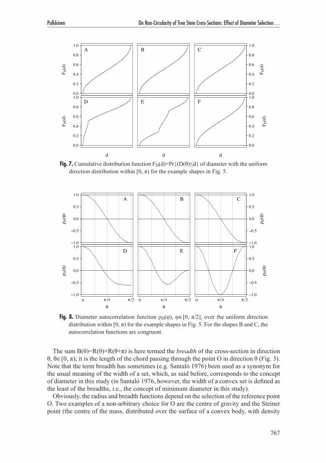
The sum B(θ)=R(θ)+R(θ+π) is here termed the breadth of the cross-section in direction θ, θ∈[0, π); it is the length of the chord passing through the point O in direction θ (Fig. 3). Note that the term breadth has sometimes (e.g. Santaló 1976) been used as a synonym for the usual meaning of the width of a set, which, as said before, corresponds to the concept of diameter in this study (in Santaló 1976, however, the width of a convex set is defined as the least of the breadths, i.e., the concept of minimum diameter in this study).

Obviously, the radius and breadth functions depend on the selection of the reference point O. Two examples of a non-arbitrary choice for O are the centre of gravity and the Steiner point (the centre of the mass, distributed over the surface of a convex body, with density

Fig. 7. Cumulative distribution function FD(d)=Pr{(D(θ)≤d} of diameter with the uniform direction distribution within [0, π) for the example shapes in Fig. 5.

−1.0

−0.5

0.0

0.5

1.0A

ρ D(φ

)

B

−1.0

−0.5

0.0

0.5

1.0C

ρ D(φ

)

0 π 4 π 2−1.0

−0.5

0.0

0.5

1.0D

ρ D(φ

)

φ0 π 4 π 2

E

φ0 π 4 π 2

−1.0

−0.5

0.0

0.5

1.0F

ρ D(φ

)

φ

Fig. 8. Diameter autocorrelation function ρD(φ), φ∈[0, π/2], over the uniform direction distribution within [0, π) for the example shapes in Fig. 5. For the shapes B and C, the autocorrelation functions are congruent.

0.0

0.2

0.4

0.6

0.8

1.0A

F D(d

)

B

0.0

0.2

0.4

0.6

0.8

1.0C

F D(d

)

d

0.0

0.2

0.4

0.6

0.8

1.0D

F D(d

)

d

E

d

0.0

0.2

0.4

0.6

0.8

1.0F

F D(d

)

768


equal to the Gaussian curvature; see Hazewinkel 1992). Given O, the radius function, as opposed to the diameter function, determines the shape of the cross-section uniquely; further, if O is the centre of gravity of the cross-section, the radius function being constant implies that the cross-section be a circle (Matérn 1956, Santaló 1976, Stoyan and Stoyan 1994).

769


3 Estimation of Cross-Section AreaIn this chapter, we consider estimating the area of a tree stem cross-section with the circle area formula and somehow selected diameters; each area estimator is thus characterised by the diameter selection method, comprising both the way in which the diameters are selected and the way in which the selected diameters are combined (typically averaged) into the circle formula input. We study how variation in diameter within a non-circular cross-section is reflected to area estimates produced by different estimators; ultimately, we want to find out what can be said about the performance of different estimators without assuming anything about the shape of a cross-section. In the end, we briefly discuss area estimation based on radii.

3.1 Foundations: Source of Randomness and Measures of Estimator Performance

Within a cross-section, we regard the randomness in an area estimator as arising from the procedure of selecting diameters from a fixed, albeit infinite, “diameter population” (cf. the discussion in Chapter 2). Measuring a diameter in a direction sampled from the uniform distribution over [0, π) means carrying out simple random sampling in the diameter popula-tion, whereas taking a diameter in a direction sampled from some non-uniform distribution means performing random sampling with unequal selection probabilities. Further, measur-ing an additional diameter perpendicular, or at any fixed angle, to a random diameter is systematic sampling with a random starting point. Yet, naturally, the diameter selection need not involve any randomness at all: taking fixed diameters, such as the maximum or the minimum diameter, or the mean diameter (the girth measurement divided by π), is just selective sampling that entails no randomness when carried out in a fixed diameter popula-tion. The area estimators based on a sample of random diameters are of course also random variables, whereas non-randomly selected diameters result in non-random area estimators when viewed from within a cross-section.

The sampling distribution of an area estimator within a cross-section is determined with respect to the diameter sampling design, that is, over all possible samples of diameters. If we select diameters by sampling their directions from a known direction distribution, we obtain the area estimator distribution via this direction distribution and the diameter function. The area estimator can be thought to be composed of a systematic part and a random part:

A(θ) = Eθ[A(θ)] + ε(θ) , (13)

where Eθ[Â(θ)] is the within-cross-section expectation of the area estimator taken over the diameter direction distribution and ε(θ) is a random error term with zero expectation (and with the distribution determined by the diameter direction distribution and the diam-eter function). The argument θ here refers to the source of randomness in general; it can be thought of, for example, as a random vector containing the directions of the diameters included in the estimator.

The area estimation error now consists of the bias of the estimator and of the random error term:

A(θ)− A = {Eθ[A(θ)]− A} + ε(θ) . (14)

The bias, measuring how far the expected value of the estimator is from the true area, rep-resents the systematic error associated with the estimator; note that this is the “mean error”

770


to be expected over repeated diameter samplings within a cross-section, not an error being realised in each individual sampling. The random error term, in turn, stands for the sampling error resulting from the fact that a diameter sample does not perfectly represent the diameter population but that there is variation between diameter samples that causes variation in esti-mator values. The usual measure for the magnitude of the sampling error ε(θ), also termed the precision of the estimator, is its variance or standard deviation. The mean squared error

Eθ{[A(θ)− A]2} = {Eθ[A(θ)]− A}2 + Eθ[ε(θ)2]

= {Eθ[A(θ)]− A}2 + Varθ[A(θ)] (15)

combining the squared bias with the precision is a commonly used measure for the accuracy of an estimator (e.g. Lindgren 1976).

Trivially, non-random area estimators — those based on girth or fixed diameters, for example — are unaffected by sampling errors: for them, Eθ[Â(θ)]=Â(θ) and Varθ[Â(θ)]=0, and the mean squared error is reduced to the squared bias, that is, to the squared estimation error [Â(θ)–A]2.

An alternative to the design-based thinking discussed above could be a model-based approach where cross-sections were regarded as realisations of random figures or as sto-chastic deformations of a template curve and where stochastic models for the invariant parameters of the random contour functions were then established and estimated in empirical analysis (see e.g. Stoyan and Stoyan 1994 and Hobolth and Jensen 1999). In this thesis, however, we will examine the different area estimators expressly in a design-based way at the within-cross-section level. What was discussed above in terms of diameter-based estimators naturally apply to radius-based estimators as well.

3.2 Effect of Non-Convexity

As already mentioned in Chapter 2, the difference AC–A between the convex area and the true area of a cross-section is always nonnegative. Aptly, Matérn (1956) termed this dif-ference the convex deficit of a cross-section.

From the practical point of view, non-convexity is rather an insidious source of error, since it cannot be observed by a girth tape or a caliper commonly used for measuring standing trees. Thus nothing besides non-negativity can be inferred about convex deficit in an ordinary area estimation situation. It then becomes a valid question whether we had better use the convex area, instead of the true area, as the reference when computing the within-cross-section bias of an area estimator.

3.3 Estimators Based on Diameters and Circle Area Formula

As suggested many times above, an intuitively appealing and the most commonly used way to estimate cross-section area is to apply the circle area formula

A = π4

D2 , (16)

where D is the diameter of the circle that the cross-section is assumed to equate with. As already discussed, D can be chosen in a number of ways within a cross-section. Firstly,

771


D may be a single measurable diameter: either random, that is, a diameter the direction of which is a random variable usually chosen to be uniformly distributed over [0, π); or systematically sampled, such as the diameter perpendicular to a random diameter; or fixed, such as the minimum diameter or the maximum diameter or the mean diameter derived from the convex perimeter. Secondly, D may be the arithmetic, geometric, or quadratic mean of two or more randomly or systematically sampled or fixed diameters. Using the geometric mean of two diameters in the circle area formula implies the assumption of ellipticity, as this estimator yields the area of an ellipse with the axis lengths equal to the diameters used in the geometric mean. Employing the quadratic mean of two or more diameters, in turn, corresponds to estimating the area as the arithmetic mean of the areas of the circles that have the diameters used in the quadratic mean. Thirdly, D may as well be some other expression constructed from random and non-random diameters, such as the “diameter” involved in the area estimator where the geometric or the quadratic mean of two or more area estimators of the types mentioned above is written in the form of a circle area formula (Matérn 1956, 1990, Loetsch et al. 1973, Kärkkäinen 1974, 1975a, 1984).

In this study, we confine ourselves to estimators where D is a single measurable diameter or a mean of two or more measurable diameters. About the mutual relations between the three types of means, it is useful to remember the following two results: First, for positive variables Xi, i=1, ..., n,

Xii=1

n

∏⎛⎝⎜⎞⎠⎟

1n

≤ 1n

Xii=1

n

∑ ≤ 1n

Xi2

i=1

n

∑ ,

(17)

that is, the geometric mean of is never greater than the arithmetic mean, which in turn is never greater than the quadratic mean (see Hardy et al. 1988 for the proofs); the equality between the means holds if all the variables Xi are equal. This implies that the area estimate given by the circle area formula with the geometric mean of unequal diameters be always less than the estimate obtained with the arithmetic mean of the same diameters, which in turn be always less than the estimate obtained with the quadratic mean of the diameters. Second, in the case of two positive variables X1 and X2, there exists the following relation between the squares of the quadratic, arithmetic and geometric means:

X12 + X2

2

2− 2

X1 + X2

2⎛⎝⎜

⎞⎠⎟

2

+ X1X2 = 0 .

(18)

This implies that the area estimate based on one of the three diameter means be straight-forwardly obtained from the estimates based on the other two (Matérn 1956).

3.3.1 Girth Diameter: Mean Diameter Derived from Convex Perimeter

The non-random area estimator

A0 =π4µD

2 = C2

4π , (19)

where the mean diameter μD=C/π (over the uniform direction distribution) derived from the convex perimeter C of the cross-section, termed here the girth diameter, is substituted

772


in the circle area formula, yields the area of the isoperimetric circle, that is, the area of the circle that has the perimeter equal to the convex perimeter of the cross-section.

For a non-circular cross-section, this estimator overestimates the convex area irrespec-tive of the shape of the cross-section, because the circle has the largest area among the isoperimetric figures in plane (Hadwiger 1957). Matérn (1956) termed the nonnegative difference Â0–AC the isoperimetric deficit of a cross-section. Regardless of the shape of a cross-section, this deficit can be shown to have the following lower bound depending on diameter variance σD2 within the cross-section:

A0 − AC ≥3π4σD

2 (20)

(see Matérn 1956 for the proof).Interestingly, Â0 serves as a baseline for many estimators based on random diameters: in

cross-sections with nonnegative correlation between perpendicular diameters, the overes-timation error in Â0 is a lower bound for the within-cross-section bias in those estimators, as we will see in the next section.

3.3.2 Random Diameters with Uniform Direction Distribution

Estimators Involving One or Two Diameters

In the way paved by Matérn (1956), we next consider the area estimators that are of the same form

A = π4

D(⋅)2 , (21)

but where D(·) is now1. random diameter D(θ), θ~Uniform(0, π) (Â1)2. arithmetic mean of a random diameter D(θ) and the diameter D(θ+π/2) perpendicular to it (Â2)3. geometric mean of D(θ) and D(θ+π/2) (Â3)4. arithmetic mean of two independent random diameters D(θ1) and D(θ2), θ1, θ2~Uniform(0, π)

i.i.d. (Â4)5. geometric mean of D(θ1) and D(θ2) (Â5).

First we focus on the systematic errors, that is, on the within-cross-section biases of these estimators. With the notation introduced before — μD denoting the diameter mean, σD2 denoting the diameter variance, and ρD(π/2) denoting the correlation between perpendicular diameters within a cross-section — the expectations of the estimators over the uniform diameter direction distribution become as follows:

E(A1) = π4µD

2 + π4σD

2

= A0 +π4σD

2 ,

(22)

773


E(A2 ) = π4µD

2 + π8σD

2 1 + ρD

π2

⎛⎝⎜

⎞⎠⎟

⎡

⎣⎢

⎤

⎦⎥

= A0 +π8σD

2 1 + ρD

π2

⎛⎝⎜

⎞⎠⎟

⎡

⎣⎢

⎤

⎦⎥ ,

(23)

E(A3) = π4µD

2 + π4σD

2 ρD

π2

⎛⎝⎜

⎞⎠⎟

= A0 +π4σD

2 ρD

π2

⎛⎝⎜

⎞⎠⎟

,

(24)

E(A4 ) = π4µD

2 + π8σD

2

= A0 +π8σD

2 ,

(25)

and

E(A5) = π4µD

2

= A0

(26)

(cf. Matérn 1956, 1990). (The expectations are obtained by writing the area estimators as sums of squared diameters and diameter products, by taking the expectations separately on each term in the sum, and by applying to these the usual rules that relate means, variances and cor-relations to each other: E[D(θ)2]=E[D(θ+π/2)2]=μD2+σD2, E[D(θ)D(θ+π/2)]=μD2+σD2ρD(π/2), E[D(θ1)D(θ2)]=E[D(θ1)]E[D(θ2)]=μD2.) Clearly, the estimator Â0 based on the convex perim-eter of a cross-section, which in the previous section was found to overestimate the convex area of a cross-section, now makes a convenient reference. Interestingly, the estimator Â5 based on the geometric mean of two independent random diameters comprises a bias equal to that of the estimator Â0. Moreover, the bias of the estimator Â2 is the arithmetic mean of the biases of the estimators Â1 and Â3 (Matérn 1956). In Table 2, the expectations of the estimators are given for the six example shapes of Fig. 5.

Table 2. Expectations of the area estimators Â0–Â4 (Eqs. 19 and 22–25) for the shapes in Fig. 5, expressed in permille of true area (cf. Matérn 1956). The expectation of the estimator Â5 is equal to Â0 (Eq. 26).

Shape A B C D E F

Â0/A (‰) 1019 1019 1022 1017 1030 1030E(Â1)/A (‰) 1025 1025 1024 1020 1034 1032E(Â2)/A (‰) 1019 1019 1022 1018 1032 1032E(Â3)/A (‰) 1013 1013 1020 1016 1030 1032E(Â4)/A (‰) 1022 1022 1023 1019 1032 1031

774


The mutual ranking of the estimators in terms of bias obviously depends on the values of σD2 and ρD(π/2) within a cross-section. With the condition σD2>0 — that is, orbiforms excluded — and by recalling that –1≤ρD(π/2)≤1, we can compose the following ρD(π/2)-dependent comparisons between the estimator expectations:

ρD(π/2)=–1: E(Â3) < Â0 = E(Â5) = E(Â2) < E(Â4) < E(Â1)–1<ρD(π/2)<0: E(Â3) < Â0 = E(Â5) < E(Â2) < E(Â4) < E(Â1)ρD(π/2) = 0: Â0 = E(Â5) = E(Â3) < E(Â4) = E(Â2) < E(Â1)0<ρD(π/2)<½: Â0 = E(Â5) < E(Â3) < E(Â4) < E(Â2) < E(Â1)ρD(π/2)=½: Â0 = E(Â5) < E(Â4) = E(Â3) < E(Â2) < E(Â1)½<ρD(π/2)<1: Â0 = E(Â5) < E(Â4) < E(Â3) < E(Â2) < E(Â1)ρD(π/2)=1: Â0 = E(Â5) < E(Â4) < E(Â3) = E(Â2) = E(Â1)

We find here that with the nonnegative values of ρD(π/2), all the estimators have expecta-tions greater or equal to that of Â0; in consequence, all the estimators yield a positive bias, that is, they systematically overestimate the area of a cross-section. With the negative values of ρD(π/2) this does not hold for the estimator Â3; however, E(Â3) attains its smallest value when ρD(π/2)=–1, and by combining this minimum with the lower bound previously obtained for Â0 (Eq. 20) we get

E(A3) ≥ A0 −π4σD

2 ≥ AC +3π4σD

2⎛⎝⎜

⎞⎠⎟− π

4σD

2 = AC +π2σD

2 , (27)

which shows that also Â3 always systematically overestimates the convex area of a cross-section (Matérn 1956). We hence conclude that regardless of the shape of a non-circular cross-section all these estimators systematically overestimate the convex area of the cross-section. In the case of orbiforms this conclusion also stands, since a circle is the largest in area among the orbiforms (cf. Fig. 4). (Note that this systematic overestimation motivates the omission of the estimators based on the quadratic mean of diameters, which yield the largest estimates by definition, from our considerations.)

The comparison above also shows that regardless of the value of ρD(π/2) and thus irrespective of the shape of a cross-section, the estimator Â1 based on only one random diameter yields the largest bias. The best strategy in terms of bias minimisation, however, depends on the shape of a cross-section: with negatively correlated perpendicular diameters (–1<ρD(π/2)<0), the use of the geometric mean is preferred and, given this, the second diameter is recom-mended to be taken at right angles to the first one instead of picking it randomly; with mildly positively correlated perpendicular diameters (0<ρD(π/2)<½), the preference of the geometric mean still pertains, but now the second diameter is more advisable to be taken independently at random direction; and finally, with the highly positively correlated per-pendicular diameters (½<ρD(π/2)<1), the priority is given to measuring both the diameters independently at random directions, and, conditional on this, to employing the geometric mean. The equalities in the change points are also interesting: if ρD(π/2)= –1 (ellipse-like cross-sections, cf. shapes A–C in Fig. 5 and Table 2), employing the arithmetic mean of two perpendicular diameters is equivalent, in terms of bias, of using the geometric mean of two random diameters; if ρD(π/2)=0 (cf. shape E in Fig. 5 and Table 2), the way of choosing diameters does not matter, but the estimators based on the same type of mean yield an equal bias; if ρD(π/2)=½, using the geometric mean of two perpendicular diameters equals, in terms of bias, using the arithmetic mean of two random diameters; and, if ρD(π/2)=1 (square-like cross-sections, cf. shape F in Fig. 5 and Table 2), the estimators based on two perpendicular diameters yield as large a bias as the estimator based on only one random diameter.

775


The optimal selection of an estimator may, however, contribute to bias reduction only marginally, since, quoting Matérn (1956), “the average difference between the ‘worst’ and the ‘best’ estimate cannot be greater than the average difference between the ‘best’ estimate and the area of the convex closure”: if 0≤ρD(π/2)≤1, then Â1 is the worst and Â0 is the best estimator, and

E(A1 − A0 ) = E(A1)− A0 = A0 +π4σD

2⎛⎝⎜

⎞⎠⎟− A0 = π

4σD

2

< 3π4σD

2 = AC +3π4σD

2⎛⎝⎜

⎞⎠⎟− AC

≤ A0 − AC = E(A0 − AC ) ;

(28)

if, in turn, –1≤ρD(π/2)<0, then Â1 is the worst and Â3 is the best estimator, and

E(A1 − A3) = E(A1)− E(A3) = A0 +π4σD

2⎛⎝⎜

⎞⎠⎟− A0 +

π4σD

2 ρD

π2

⎛⎝⎜

⎞⎠⎟

⎡

⎣⎢

⎤

⎦⎥

= π4σD

2 1 − ρD

π2

⎛⎝⎜

⎞⎠⎟

⎡

⎣⎢

⎤

⎦⎥

≤ π2σD

2 = AC +π2σD

2⎛⎝⎜

⎞⎠⎟− AC

≤ E(A3)− AC = E(A3 − AC )

(29)

(in both these elaborations, Eq. 20 giving the lower bound for Â0 is employed, and in the latter derivation also Eq. 27 giving the lower bound for Â3 is used).

From the systematic errors we proceed into the sampling errors quantified by the within-cross-section variances of the estimators over the uniform direction distribution. Except for the estimator Â5 based on the geometric mean of two independent diameters, the variances cannot be expressed in terms of the simple parameters μD, σD2, and ρD(π/2), but involve higher moments and product moments of diameters, which make them somewhat difficult to compare with each other:

Var(A1) = π2

16E[D(θ)4]− µD

2 + σD2( )2{ } ,

(30)

Var(A2 ) = π2

1618

E[D(θ)4]+ 12

E D(θ)3D θ+ π2

⎛⎝⎜

⎞⎠⎟

⎡

⎣⎢

⎤

⎦⎥ +

38

E D(θ)2 D θ+ π2

⎛⎝⎜

⎞⎠⎟

2⎡

⎣⎢⎢

⎤

⎦⎥⎥

⎧⎨⎪

⎩⎪

− 14

2µD2 + σD

2 1+ ρD

π2

⎛⎝⎜

⎞⎠⎟

⎡

⎣⎢

⎤

⎦⎥

⎧⎨⎪

⎩⎪

⎫⎬⎪

⎭⎪

2 ⎫⎬⎪

⎭⎪,

(31)

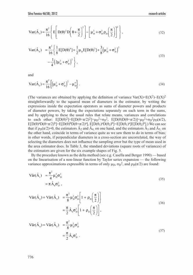
776


Var(A3) = π2

16E D(θ)2 D θ+ π

2⎛⎝⎜

⎞⎠⎟

2⎡

⎣⎢⎢

⎤

⎦⎥⎥− µD

2 + σD2 ρD

π2

⎛⎝⎜

⎞⎠⎟

⎡

⎣⎢

⎤

⎦⎥

2⎧⎨⎪

⎩⎪

⎫⎬⎪

⎭⎪ ,

(32)

Var(A4 ) = π2

1618

E[D(θ)4]+ 12µDE[D(θ)3]+ 3

8µD

2 + σD2( )2⎧

⎨⎩

− 14

2µD2 + σD

2( )2 ⎫⎬⎭

,

(33)

and

Var(A5) = π2

16µD

2 + σD2( )2

−µD4{ } .

(34)

(The variances are obtained by applying the definition of variance Var(X)=E(X2)–E(X)2 straightforwardly to the squared mean of diameters in the estimator, by writing the expressions inside the expectation operators as sums of diameter powers and products of diameter powers, by taking the expectations separately on each term in the sums, and by applying to these the usual rules that relate means, variances and correlations to each other: E[D(θ)2]=E[D(θ+π/2)2]=μD2+σD2, E[D(θ)D(θ+π/2)]=μD2+σD2ρD(π/2), E[D(θ)aD(θ+π/2)b]=E[D(θ)bD(θ+π/2)a], E[D(θ1)aD(θ2)b]=E[D(θ1)a]E[D(θ2)b].) We can see that if ρD(π/2)=0, the estimators Â2 and Â4, on one hand, and the estimators Â3 and Â5, on the other hand, coincide in terms of variance quite as we saw them to do in terms of bias; in other words, if perpendicular diameters in a cross-section are uncorrelated, the way of selecting the diameters does not influence the sampling error but the type of mean used in the area estimator does. In Table 3, the standard deviations (square roots of variances) of the estimators are given for the six example shapes of Fig. 5.

By the procedure known as the delta method (see e.g. Casella and Berger 1990) — based on the linearisation of a non-linear function by Taylor series expansion — the following variance approximations expressible in terms of only μD, σD2, and ρD(π/2) are found:

Var(A1) = π2

4µD

2 σD2

= π A0σD2 ,

(35)

Var(A2 ) = Var(A3) = π2

8µD

2 σD2 1 + ρD

π2

⎛⎝⎜

⎞⎠⎟

⎡

⎣⎢

⎤

⎦⎥

= π2

A0σD2 1 + ρD

π2

⎛⎝⎜

⎞⎠⎟

⎡

⎣⎢

⎤

⎦⎥ ,

(36)

Var(A4 ) = Var(A5) = π2

8µD

2 σD2

= π2

A0σD2 .

(37)

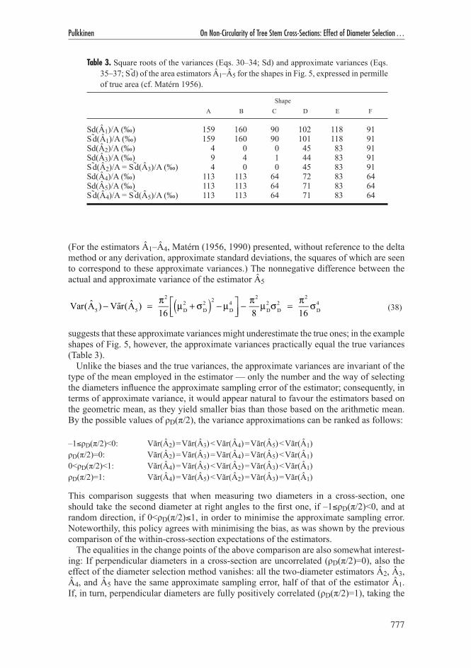
777


(For the estimators Â1–Â4, Matérn (1956, 1990) presented, without reference to the delta method or any derivation, approximate standard deviations, the squares of which are seen to correspond to these approximate variances.) The nonnegative difference between the actual and approximate variance of the estimator Â5

Var(A5)− Var(A5) = π2

16µD

2 + σD2( )2

−µD4⎡

⎣⎢⎤⎦⎥− π2

8µD

2 σD2 = π2

16σD

4 (38)

suggests that these approximate variances might underestimate the true ones; in the example shapes of Fig. 5, however, the approximate variances practically equal the true variances (Table 3).

Unlike the biases and the true variances, the approximate variances are invariant of the type of the mean employed in the estimator — only the number and the way of selecting the diameters influence the approximate sampling error of the estimator; consequently, in terms of approximate variance, it would appear natural to favour the estimators based on the geometric mean, as they yield smaller bias than those based on the arithmetic mean. By the possible values of ρD(π/2), the variance approximations can be ranked as follows:

–1≤ρD(π/2)<0: Vãr(Â2) = Vãr(Â3) < Vãr(Â4) = Vãr(Â5) < Vãr(Â1)ρD(π/2)=0: Vãr(Â2) = Vãr(Â3) = Vãr(Â4) = Vãr(Â5) < Vãr(Â1)0<ρD(π/2)<1: Vãr(Â4) = Vãr(Â5) < Vãr(Â2) = Vãr(Â3) < Vãr(Â1)ρD(π/2)=1: Vãr(Â4) = Vãr(Â5) < Vãr(Â2) = Vãr(Â3) = Vãr(Â1)

This comparison suggests that when measuring two diameters in a cross-section, one should take the second diameter at right angles to the first one, if –1≤ρD(π/2)<0, and at random direction, if 0<ρD(π/2)≤1, in order to minimise the approximate sampling error. Noteworthily, this policy agrees with minimising the bias, as was shown by the previous comparison of the within-cross-section expectations of the estimators.

The equalities in the change points of the above comparison are also somewhat interest-ing: If perpendicular diameters in a cross-section are uncorrelated (ρD(π/2)=0), also the effect of the diameter selection method vanishes: all the two-diameter estimators Â2, Â3, Â4, and Â5 have the same approximate sampling error, half of that of the estimator Â1. If, in turn, perpendicular diameters are fully positively correlated (ρD(π/2)=1), taking the

Table 3. Square roots of the variances (Eqs. 30–34; Sd) and approximate variances (Eqs. 35–37; S d) of the area estimators Â1–Â5 for the shapes in Fig. 5, expressed in permille of true area (cf. Matérn 1956).

Shape A B C D E F

Sd(Â1)/A (‰) 159 160 90 102 118 91S d(Â1)/A (‰) 159 160 90 101 118 91Sd(Â2)/A (‰) 4 0 0 45 83 91Sd(Â3)/A (‰) 9 4 1 44 83 91S d(Â2)/A = S d(Â3)/A (‰) 4 0 0 45 83 91Sd(Â4)/A (‰) 113 113 64 72 83 64Sd(Â5)/A (‰) 113 113 64 71 83 64S d(Â4)/A = S d(Â5)/A (‰) 113 113 64 71 83 64

778


second diameter at right angles to the first one benefits none compared to measuring only one diameter but the approximate variance is halved only by measuring the two diameters inde-pendently. Finally, if perpendicular diameters are fully negatively correlated (ρD(π/2)=–1), the approximate sampling error for the estimators Â2 and Â3 disappears (cf. shapes B and C in Table 3); hence, for ellipse-like cross-sections, measuring two perpendicular diameters should always lead to an approximately sampling-error-free area estimate.

Generalisation to n Diameters

The area estimators based on a mean of two diameters can naturally be generalised to involve countably many diameters. For the generalised estimators involving the arithmetic mean, the within-cross-section expectations are expressible in terms of the simple parameters μD, σD2, and ρD(π/2): the expectation of the estimator based on the arithmetic mean of n∈N, n≥2, independent random diameters (a generalisation of Â4 and thus denoted by ÂG4) becomes

E(AG 4 ) = π4µD

2 + π4n

σD2

= A0 +π4n

σD2 ,

(39)

and the expectation of the estimator based on the arithmetic mean of n/2, n=2k, k≥1, k∈N, independent random diameters and their n/2 perpendiculars (a generalisation of Â2 and thus denoted by ÂG2) is found to be

E(AG 2 ) = π4µD

2 + π4n

σD2 1+ ρD

π2

⎛⎝⎜

⎞⎠⎟

⎡

⎣⎢

⎤

⎦⎥

= A0 +π4n

σD2 1+ ρD

π2

⎛⎝⎜

⎞⎠⎟

⎡

⎣⎢

⎤

⎦⎥

(40)

(cf. the commonly known theorem about the mean of quadratic forms, to be found in e.g. Kendall and Stuart 1979). If perpendicular diameters are uncorrelated, these general esti-mators clearly coincide in terms of bias. Further, as n tends to infinity, the expectations of both the general estimators tend to Â0; the biases of the estimators can hence be reduced by measuring more diameters, but the biases can never fall below that of Â0.

The expectations of the generalised estimators based on the geometric mean of more than two diameters cannot be expressed in terms of μD, σD2, and ρD(π/2), but involve “fractional diameter moments”, that is, expectations of fractional powers of diameters over the uniform direction distribution, which make them difficult to compare with those presented above: the expectation of the estimator based on the geometric mean of n independent random diameters (a generalisation of Â5 and thus denoted by ÂG5) becomes

E(AG5) =π4E D(θ)

2n

⎡

⎣⎢

⎤

⎦⎥

⎧⎨⎪

⎩⎪

⎫⎬⎪

⎭⎪

n

,

(41)

and the expectation of the estimator based on the geometric mean of n/2 independent random diameters and their n/2 perpendiculars (a generalisation of Â3 and thus denoted by ÂG3) is found to be

779


E(AG 3) = π4

E D(θ)2n D θ+ π

2⎛⎝⎜

⎞⎠⎟

2n

⎡

⎣

⎢⎢⎢

⎤

⎦

⎥⎥⎥

⎧⎨⎪

⎩⎪

⎫⎬⎪

⎭⎪

n2

.

(42)

For the generalised area estimators based on the arithmetic mean, the variances become somewhat intricate:

Var(AG 4 ) = π2

16n4 n E[D(θ)4]+ 4n(n −1)µDE[D(θ)3]+ n(2n − 3) µD2 + σD

2( )2{ + 6n(n −1)(n − 2)− 2n2(n −1)⎡⎣ ⎤⎦µD

2 µD2 + σD

2( ) + n(n −1)(n − 2)(n − 3)− n2(n −1)2⎡⎣ ⎤⎦µD

4 } ,

(43)

and

Var(AG 2 ) = π2

16n4 n E[D(θ)4]+ 4n E D(θ)3D θ+ π2

⎛⎝⎜

⎞⎠⎟

⎡

⎣⎢

⎤

⎦⎥ + 3n E D(θ)2 D θ+ π

2⎛⎝⎜

⎞⎠⎟

2⎡

⎣⎢⎢

⎤

⎦⎥⎥

⎧⎨⎪

⎩⎪

+4n(n − 2)µD E[D(θ)3]+ 3E D(θ)2 D θ+ π2

⎛⎝⎜

⎞⎠⎟

⎡

⎣⎢

⎤

⎦⎥

⎧⎨⎪

⎩⎪

⎫⎬⎪

⎭⎪

+3n(n − 2) 2µD2 + σD

2 1+ ρD

π2

⎛⎝⎜

⎞⎠⎟

⎡

⎣⎢

⎤

⎦⎥

⎧⎨⎪

⎩⎪

⎫⎬⎪

⎭⎪

2

+6n(n − 2)(n − 4)µD2 2µD

2 + σD2 1+ ρD

π2

⎛⎝⎜

⎞⎠⎟

⎡

⎣⎢

⎤

⎦⎥

⎧⎨⎪

⎩⎪

⎫⎬⎪

⎭⎪

+ n(n − 2)(n − 4)(n − 6)µD4

− n 2µD2 + σD

2 1+ ρD

π2

⎛⎝⎜

⎞⎠⎟

⎡

⎣⎢

⎤

⎦⎥

⎧⎨⎪

⎩⎪

⎫⎬⎪

⎭⎪+ n(n − 2)µD

2⎧⎨⎪

⎩⎪

⎫⎬⎪

⎭⎪

2 ⎫⎬⎪

⎭⎪ .

(44)

For the generalisations based on the geometric mean, the variance expressions are far simpler on the face but again relatively uninformative if one wants to compare them to those above:

Var(AG5) = π2

16E D(θ)

4n

⎡

⎣⎢

⎤

⎦⎥

⎧⎨⎪

⎩⎪

⎫⎬⎪

⎭⎪

n

− E D(θ)2n

⎡

⎣⎢

⎤

⎦⎥

⎧⎨⎪

⎩⎪

⎫⎬⎪

⎭⎪

2n⎧⎨⎪

⎩⎪

⎫⎬⎪

⎭⎪ ,

(45)

and

Var(AG 3) = π2

16E D(θ)

4n D θ+ π

2⎛⎝⎜

⎞⎠⎟

4n

⎡

⎣

⎢⎢⎢

⎤

⎦

⎥⎥⎥

⎧⎨⎪

⎩⎪

⎫⎬⎪

⎭⎪

n2

− E D(θ)2n D θ+ π

2⎛⎝⎜

⎞⎠⎟

2n

⎡

⎣

⎢⎢⎢

⎤

⎦

⎥⎥⎥

⎧⎨⎪

⎩⎪

⎫⎬⎪

⎭⎪

n⎧

⎨⎪⎪

⎩⎪⎪

⎫

⎬⎪⎪

⎭⎪⎪

.

(46)

780


Contrary to these actual variances, the delta method approximations are both uncomplicated and interpretative:

Var(AG 4 ) = Var(AG5) = π2

4nµD

2 σD2

= πn

A0σD2 ,

(47)

and

Var(AG 2 ) = Var(AG 3) = π2

4nµD

2 σD2 1+ ρD

π2

⎛⎝⎜

⎞⎠⎟

⎡

⎣⎢

⎤

⎦⎥

= πn

A0σD2 1+ ρD

π2

⎛⎝⎜

⎞⎠⎟

⎡

⎣⎢

⎤

⎦⎥ .

(48)

Trivially, by measuring more diameters one reduces the true and the approximate variances of the generalised estimators, up to zero as n tends to infinity. Otherwise the generalised estimators share the properties previously demonstrated for the two-diameter estimators: If perpendicular diameters are uncorrelated in a cross-section, the generalised estimators coincide pairwise in terms of true sampling errors (Var(ÂG3)=Var(ÂG5), Var(ÂG2)=Var(ÂG4)) and all together in terms of approximate sampling errors (Vãr(ÂG3)=Vãr(ÂG5)=Vãr(ÂG2) =Vãr(ÂG4)). Further, in the case of an elliptic cross-section, for which ρD(π/2) is near –1, the approximate variances of ÂG2 and ÂG3 become close to zero independent of the value of n, and thus increasing the number of diameter measurements within the cross-section should not make much difference in terms of the approximate sampling error.

3.3.3 Minimum and Maximum Diameters

From the estimators involving random diameters with uniformly distributed directions, we proceed to discussing six fixed estimators based on the minimum and maximum diameters of a cross-section. The estimators are still of the form

A = π4

D2 ,

(49)

where D is now, following Matérn (1956),6. arithmetic mean of the minimum diameter Dmin and the maximum diameter Dmax in the cross-

section (Â6)7. geometric mean of Dmin and Dmax (Â7)8. arithmetic mean of Dmin and its perpendicular (Â8)9. geometric mean of Dmin and its perpendicular (Â9)10. arithmetic mean of Dmax and its perpendicular (Â10)11. geometric mean of Dmax and its perpendicular (Â11).

Note that the estimators Â8–Â11 may not always be well-defined — consider, for example, the situation where Dmin is attained in two different directions but the diameters perpen-dicular to these diameters are unequal (Matérn 1956). If the estimators are well-defined,

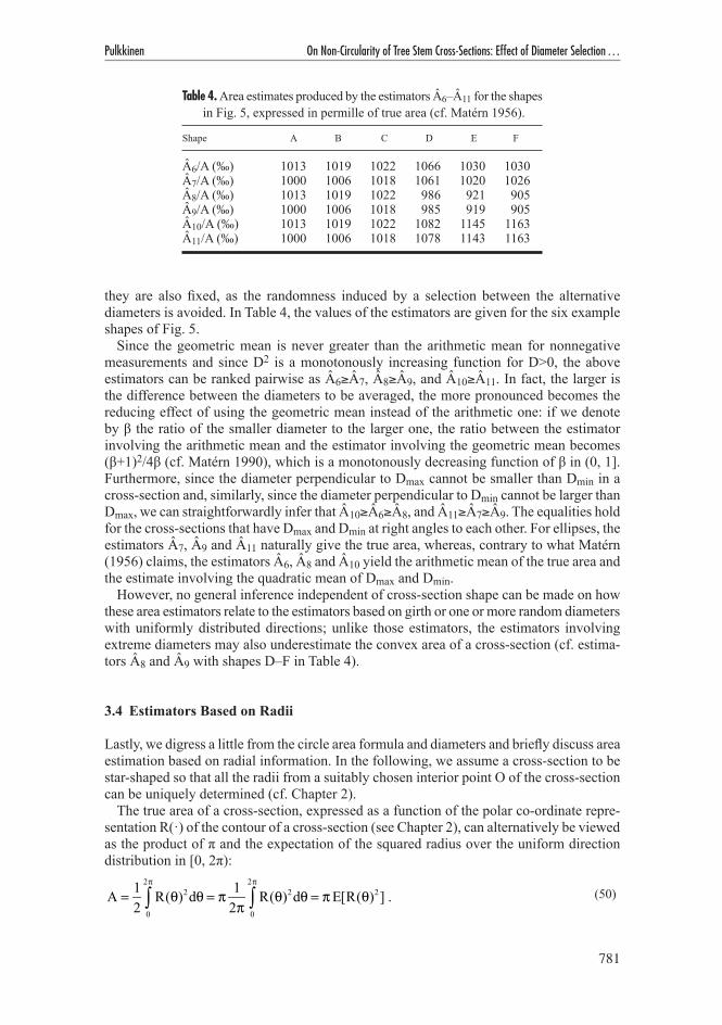
781


they are also fixed, as the randomness induced by a selection between the alternative diameters is avoided. In Table 4, the values of the estimators are given for the six example shapes of Fig. 5.

Since the geometric mean is never greater than the arithmetic mean for nonnegative measurements and since D2 is a monotonously increasing function for D>0, the above estimators can be ranked pairwise as Â6≥Â7, Â8≥Â9, and Â10≥Â11. In fact, the larger is the difference between the diameters to be averaged, the more pronounced becomes the reducing effect of using the geometric mean instead of the arithmetic one: if we denote by β the ratio of the smaller diameter to the larger one, the ratio between the estimator involving the arithmetic mean and the estimator involving the geometric mean becomes (β+1)2/4β (cf. Matérn 1990), which is a monotonously decreasing function of β in (0, 1]. Furthermore, since the diameter perpendicular to Dmax cannot be smaller than Dmin in a cross-section and, similarly, since the diameter perpendicular to Dmin cannot be larger than Dmax, we can straightforwardly infer that Â10≥Â6≥Â8, and Â11≥Â7≥Â9. The equalities hold for the cross-sections that have Dmax and Dmin at right angles to each other. For ellipses, the estimators Â7, Â9 and Â11 naturally give the true area, whereas, contrary to what Matérn (1956) claims, the estimators Â6, Â8 and Â10 yield the arithmetic mean of the true area and the estimate involving the quadratic mean of Dmax and Dmin.

However, no general inference independent of cross-section shape can be made on how these area estimators relate to the estimators based on girth or one or more random diameters with uniformly distributed directions; unlike those estimators, the estimators involving extreme diameters may also underestimate the convex area of a cross-section (cf. estima-tors Â8 and Â9 with shapes D–F in Table 4).

3.4 Estimators Based on Radii

Lastly, we digress a little from the circle area formula and diameters and briefly discuss area estimation based on radial information. In the following, we assume a cross-section to be star-shaped so that all the radii from a suitably chosen interior point O of the cross-section can be uniquely determined (cf. Chapter 2).

The true area of a cross-section, expressed as a function of the polar co-ordinate repre-sentation R(·) of the contour of a cross-section (see Chapter 2), can alternatively be viewed as the product of π and the expectation of the squared radius over the uniform direction distribution in [0, 2π):

A = 12

R0

2π

∫ (θ)2dθ = π 12π

R0

2π

∫ (θ)2dθ = πE[R(θ)2] . (50)

Table 4. Area estimates produced by the estimators Â6–Â11 for the shapes in Fig. 5, expressed in permille of true area (cf. Matérn 1956).

Shape A B C D E F

Â6/A (‰) 1013 1019 1022 1066 1030 1030Â7/A (‰) 1000 1006 1018 1061 1020 1026Â8/A (‰) 1013 1019 1022 986 921 905Â9/A (‰) 1000 1006 1018 985 919 905Â10/A (‰) 1013 1019 1022 1082 1145 1163Â11/A (‰) 1000 1006 1018 1078 1143 1163

782


These expressions suggest an area estimator of the type

A = 12

R(θi )2 2π

n⎡

⎣⎢

⎤

⎦⎥

i=1

n

∑ = πn

R(θi )2

i=1

n

∑ , (51)

where R(θi) is the radius of a cross-section measured in direction θi, i=1, 2, ..., n. In the first expression, the definite integral of R(θ)2 is obviously approximated by the sum of n rectangles with the width 2π/n and the height R(θi)2. This corresponds to estimating the area of the cross-section with the sum of n disjoint, equally wide circular sectors (the area of a circular sector with angle Δθi=2π/n and side length R(θi) is ΔθiR(θi)2/2=πR(θi)2/n, and summing up n such sectors then results in the second expression). This expression is straight-forwardly seen to be π times the squared quadratic mean of n radii R(θi), a natural estimator for π times the expectation of the squared radius over the uniform direction distribution. The application of this estimator does not require that the radii be measured equidistantly.

Just as the diameters in the estimators based on the circle area formula can be chosen in many ways, also for the radii various selection strategies are naturally available (see e.g. Gregoire and Valentine 1995). The remarkable property of the estimator of Eq. 51 is that it is unbiased if the marginal distribution of each radius direction θi is uniform over [0, 2π) (Matérn 1956, Gregoire and Valentine 1995). This condition naturally holds if the directions are independently sampled from the uniform distribution over [0, 2π), in which case it is also easy to derive analytically the exact variance for the estimator and also to find an unbiased estimator for that variance (Gregoire and Valentine 1995). However, the variance is directly related to the variation in the radii used and thus considerably affected by the choice of the location of O; for decreasing the variance of the estimator, centralising the location of O as well as applying systematic sampling strategies for radii have been suggested (Gregoire and Valentine 1995).

In sum, the bias in area estimation can be avoided, if the cross-sections can be observed “from inside” instead of “from outside”, that is, if radii instead of diameters can be meas-ured. For standing trees this is not feasible with the standard measurement equipment, but to estimating the area of end sections of logs — or the area of the crown projection of a tree — for instance, this approach certainly pertains (Matérn 1956).

783


4 Bitterlich SamplingBitterlich sampling — also referred to as relascope sampling, angle-count sampling, horizon-tal point sampling, variable radius plot sampling, and plotless sampling — was introduced in forestry by the Austrian forester Walter Bitterlich (1948a, 1948b) as a simple counting technique for estimating relative basal area of a tree stand. Nowadays it is also extensively used for sampling trees in forest inventories. The idea in the method is to count, or pick into the sample, those trees in a stand that subtend an angle greater or equal to a fixed angle α when viewed horizontally at breast height from a randomly located point in the stand (Fig. 9). An estimate for the relative basal area at breast height is then obtained by simply multiplying the tally of trees by an α-dependent constant. The procedure may be repeated at several randomly located viewing points in the stand.

There are several alternative ways to formalise Bitterlich sampling. In a model-based approach, the sampling procedure is considered under a model assumed for the structure of the tree stand: in such a model, tree locations are typically regarded as a realisation of a (stationary) spatial point process and tree diameters are treated either as independent random variables with assumed (identical) probability distributions or as the marks of the point process with a mark distribution function involving spatial dependence between the trees; the viewing points need not then be randomly located, but the statistical properties of the estimators of stand totals (typically relative basal area or stem volume) based on angle-count samples are derived given the assumed model (e.g. Holgate 1967, Sukwong et al. 1971, Matérn 1972, Oderwald 1981, and Penttinen 1988). In this study, however, we adopt the usual design-based approach (refer to common textbooks such as e.g. de Vries 1986, Schreuder et al. 1993, and Gregoire and Valentine 2008), where the spatial pattern of tree locations in the region of interest is regarded as fixed and where the randomness in estimators is considered to arise only from the choice of the viewing point locations. Within this design-based context, there are then at least three different unequal probability sample designs for finite population and one formulation for infinite population to choose among (Eriksson 1995); these differ from each other by the definition of sampling unit and population — whether the sampling unit is considered to be the area from which a tree is seen by relascope, the actual tree, or the viewing point in which relascope is used, and,

Fig. 9. Selection of trees in region L by Bitterlich sampling with viewing angle α: the trees (white cross-sections) that subtend an angle greater or equal to α, when viewed at breast height from a randomly selected point Q in L, are included in the sample. The inclusion region Mi(α) of the tree i with diameter Di is outlined with the dashed line.

784


accordingly, whether the population to be sampled then becomes finite or infinite. In this study, we adhere to the classical Grosenbaugh design.

In the Grosenbaugh design, the population is finite and consists of the trees reaching above the breast height in the region of interest. A sample is then composed of the trees selected at one randomly located viewing point, and sampling at k independently randomly located viewing points in the region results in k independent samples. The probability of being included in a sample, termed the inclusion probability — which in this case equals the probability of being selected at each view, referred to as the selection probability — varies according to tree. More precisely — and first realised by the American forester Lewis R. Grosenbaugh (1958), hence the name of the design (Eriksson 1995) — Bitterlich sampling is a method of PPS sampling, that is, sampling with probability proportional to size, meaning that each sampling unit is included in a sample with probability proportional to a covariate, in this case the cross-section area at breast height, which is positively correlated with the variable of interest, in this case typically stem volume.

The estimation of population totals in PPS sampling relies upon the Horvitz-Thompson theorem, which is a beautifully general theory for design-based inference from probability samples (Overton and Stehman 1995). The Horvitz-Thompson estimation is based on the inclusion probabilities of the sampling units, by the inverses of which the observed values of the characteristics of interest are weighted. The theorem is explained in more detail in Appendix B.

Our interest focuses on how non-circularity in the breast height cross-sections of trees affects stand or tree characteristic estimation based on Bitterlich sampling. In order to avoid the complications irrelevant from this point of view, we make the following three assump-tions, which are independent of our chosen sampling strategy consisting of the Grosen-baugh design and the Horvitz-Thompson estimator: First, we assume the ground level to be horizontal. Second, we assume the viewer’s eye to be at breast height (1.3 m) from the ground level and the viewer to sight trees horizontally. And third, we assume the region of interest to be such that the edge effects on the inclusion probabilities of trees need not be considered (for example, we assume the borders of the region to be set in the manner that each tree taken to belong to the stand is located farther than its inclusion radius (Eq. 52) from the borders; for some methods of dealing with the edge effect in Bitterlich sampling, see Grosenbaugh 1958, Haga and Maezawa 1959, Barrett 1964, and Schmid 1969).

4.1 Estimation of Stand Totals

We start by explaining how stand totals, that is, sums of tree characteristics within a stand, are estimated from a Bitterlich sample of trees, when the tree cross-sections at breast height are circular. Then we investigate the errors that emerge when the estimators based on the circularity assumption are applied to trees with non-circular of cross-sections. Finally, we examine the estimation of relative basal area in both these aspects.

In addition to the general simplifying presumptions stated above, we assume the char-acteristics of the trees in the sample to be measured or estimated without error. For the notation, let L denote the region of interest in the ground plane, |L| the area of this region, and I the set of the trees growing in L and reaching above breast height. Further, let Q denote a uniformly randomly located viewing point in L and α∈(0, π) the viewing angle used in a relascope.

785


4.1.1 Principle under Assumption of Circular Cross-Sections

If the cross-sections of the trees are circular at breast height, the maximum distance, deter-mined from the tree pith, at which the tree i∈I with breast height diameter Di is taken into the Bitterlich sample becomes

ri(α) =Di

2⋅ 1sin(α / 2)

(52)

by a straightforward trigonometric consideration (Fig. 9). In other words, the inclusion region Mi(α) within which the tree i∈I is observed in an angle greater or equal to α is a circle with radius ri(α) and area

|Mi (α) | = π ri(α)2 = π4Di2 ⋅ 1sin2(α / 2)

(53)

(Fig. 9). The ratio κi(α) of the cross-section area to the inclusion area for tree i∈I is now seen to depend only on the viewing angle α and thus have the same value for all the trees in I:

κ i (α) =

π4

Di2

|Mi (α) |= sin2(α / 2) ; (54)

the ratio is referred to as the basal area factor. (Note that the cross-section area and inclu-sion area are here assumed to be expressed in the same units, so that the units cancel out in sin2(α/2); to express the basal area factor in m2/ha or ft2/ac, sin2(α/2) has to be multiplied with 10 000 or 43 560, respectively.)

The inclusion probability πi(α) of a tree i∈I is the probability that the viewing point Q is located in the inclusion region Mi(α); on account of the uniform distribution of Q in L, the probability is given by the simple area ratio

π i (α) =|Mi (α) |

|L |= π

4Di

2 ⋅ 1sin2(α / 2) |L |

. (55)

(Note that the inclusion region is here defined to contain the ground-level cross-section of the stem, although the viewing point Q cannot be located within the cross-section.) Accordingly, the probability of a tree to be included in a sample is proportional to its cross-section area (squared diameter) at breast height and inversely proportional to the area of the region of interest; further, the smaller the viewing angle (and, consequently, the smaller the basal area factor) the larger the probability, as sin2(α/2) is monotonously increasing for α∈(0, π).

Let now sQ(α)⊆I denote the sample of trees obtained with the relascope angle α at the viewing point Q∈L. From each tree i in sQ(α), we measure the breast height diameter Di and the value Yi of the characteristic of interest. As is apparent from Eq. 55, we need the diameter measurements for the inclusion probabilities of the sample trees, which then enable us to apply the Horvitz-Thompson theorem for an unbiased estimation of the total amount of the characteristic of interest in the region L. The sum Y=Σi∈IYi is estimated by

786


YHT =Yi

π i (α)i∈sQ (α )∑

= |L | sin2(α / 2)Yi

π4

Di2i∈sQ (α )

∑ , (56)

that is, as a weighted sum of the sample tree measurements with the inverses of the cross-section areas (squared diameters) as weights and with a quantity depending on the viewing angle (or the basal area factor) and the area of the region of interest as the scaling coefficient.

The randomness in ŶHT stems from the placement of the viewing point Q in the region L, as this determines the sample sQ(α). By the Horvitz-Thompson theorem (Appendix B), ŶHT is unbiased with respect to the sampling design, that is, E(ŶHT)=Y, where the expecta-tion is taken over the probability distribution of all possible samples sQ(α) resulting from all possible locations of Q.

The variance of ŶHT depends on the spatial pattern of the trees in the stand, as it involves the joint inclusion probabilities for all the pairs of the trees in the population (Appendix B). The joint inclusion probability πij(α) for trees i, j∈I is the probability that both the trees are included in a sample, and in Bitterlich sampling this probability is proportional to the overlapping area of the tree inclusion regions. For the unbiased variance estimator given in Appendix B (Eq. B9) and based on a sample of trees taken at one viewing point, these probabilities need not only be known but also positive for all the pairs of trees in the sample. In a Bitterlich sample, the positivity requirement is invariably fulfilled, as the inclusion regions of the trees in the same sample necessarily overlap. The requirement of knowing the spatial pattern of the trees in the sample can be circumvented by repeating Bitterlich sampling at k randomly and independently selected viewing points Qj∈L, j=1, ..., k: The estimators ŶHT[sQj(α)] obtained from the k samples are independent and identically distributed, and hence have the same variance Var{ŶHT[sQj(α)]}≡Var(ŶHT) for all Qj. An unbiased estimator for this variance is given by the sample variance of the k estimators:

Var(YHT ) = 1k −1

YHT[sQj(α)]− YHT{ }2

j=1

k

∑ , (57)

where YHT is the mean of the k independent estimators ŶHT[sQj(α)]. The population total Y is estimated with YHT, the variance of which is Var(YHT)=Var(ŶHT)/k. An unbiased estimator of the variance of YHT then becomes

Var(YHT ) = 1k

Var[YHT]

= 1k(k −1)

YHT[sQj(α)]− YHT{ }2

j=1

k

∑

(58)

(cf. de Vries 1986, Schreuder et al. 1993, Eriksson 1995, Gregoire and Valentine 2008). A model-based approach provides an alternative way of estimating the variance of a

stand total estimator — in fact, the model-based studies referred to in the beginning of this chapter expressly address this problem. Under a certain class of models for the random mechanism generating forest stands, analytical expressions for the variance can be found; under other models, the variance can be estimated via simulations.

787


4.1.2 Effect of Non-Circularity of Cross-Sections

Since Bitterlich sampling operates with the tangents of the convex closures of breast height cross-sections, non-convexity in the cross-sections is unobservable and thus does not influence the selection of trees. Therefore, when examining how non-circularity in the breast height cross-sections of trees affects stand total estimation by Bitterlich sampling, we confine our-selves to considering the convex closures of the cross-sections of arbitrary non-circular shape.

If the convex closure of the breast height cross-section of a tree i∈I is not a circle, the maximum distance at which the tree is counted with a certain viewing angle α varies by the direction in which the tree is being viewed. Ergo, the inclusion region becomes non-circular (Fig. 10; cf. Grosenbaugh 1958, Bitterlich 1984). The size and shape of the inclusion region depend not only on the size and shape of the breast height cross-section but also on the view-ing angle α used (Fig. 11). Using the support function pi(·) of the breast height cross-section in tree i, now defined in a co-ordinate system with the origin set in the centre of gravity of the convex closure of the cross-section (or in the pith of the cross-section), we attain the following parametric representation for the length of the radius of the inclusion region:

ri(θ; α) = 1sinα

pi(θ)2 + pi(θ+ π −α)2 + 2pi(θ)pi(θ+ π −α)cosα , (59)

where α∈(0, π) and θ∈[0, 2π) (see Appendix C for the derivation). (Note that in this para-metrisation, θ does not indicate the direction of the radius, but the direction is a function of θ and α (Appendix C); consequently, the area of the inclusion region is not obtained straightforwardly by integrating ri(θ; α)2 from 0 to 2π (cf. Eq. 12 in Chapter 2).) We see that as α tends to zero, the numerator of ri(θ; α) tends to pi(θ)+pi(θ+π)=Di(θ) (and the denomi-nator tends to 0); accordingly, for the trees with an orbiform breast height cross-section (constant diameter function D(·) at breast height), the limiting shape of the inclusion region is a circle (e.g. Fig. 11 B). As α tends to π, the viewer draws closer and closer to the stem, and the radii ri(θ; α) are finally found to tend to the radii of the convex closure of the breast height cross-section; in other words, the inclusion region tends to the convex closure of the breast height cross-section (cf. Matérn 1956, p. 24).

A B C

D E F

Fig. 10. Inclusion regions obtained with the viewing angle α=20° for five of the six example shapes discussed in Chapter 2 (A and C–F in. Fig. 5 and Table 1) and for an orbiform (B, cf. Fig. 4). The dashed line indicates the inclusion region of the circle that has the same area as the cross-section.

A B C

D E F

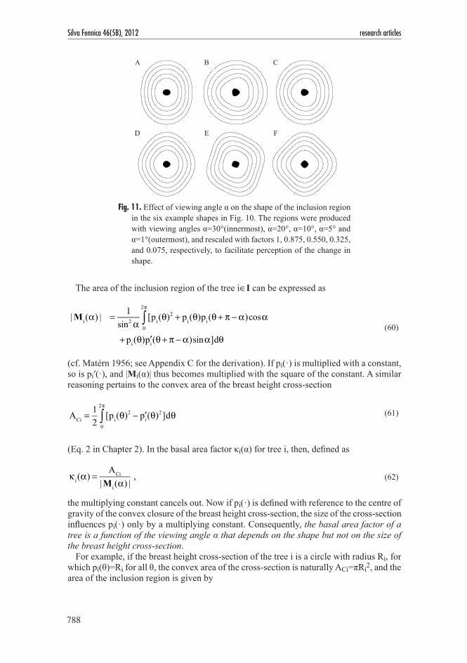
788


The area of the inclusion region of the tree i∈I can be expressed as

|Mi (α) | = 1sin2 α

[pi(θ)2 + pi(θ)pi(θ+ π −α)cosα0

2π

∫ + pi(θ) ′pi(θ+ π −α)sinα]dθ

(60)

(cf. Matérn 1956; see Appendix C for the derivation). If pi(·) is multiplied with a constant, so is pi′(·), and |Mi(α)| thus becomes multiplied with the square of the constant. A similar reasoning pertains to the convex area of the breast height cross-section

ACi =12[pi(θ)

2 − ′pi(θ)2]dθ

0

2π

∫

(61)

(Eq. 2 in Chapter 2). In the basal area factor κi(α) for tree i, then, defined as

κ i (α) =ACi

|Mi (α) | , (62)

the multiplying constant cancels out. Now if pi(·) is defined with reference to the centre of gravity of the convex closure of the breast height cross-section, the size of the cross-section influences pi(·) only by a multiplying constant. Consequently, the basal area factor of a tree is a function of the viewing angle α that depends on the shape but not on the size of the breast height cross-section.

For example, if the breast height cross-section of the tree i is a circle with radius Ri, for which pi(θ)=Ri for all θ, the convex area of the cross-section is naturally ACi=πRi2, and the area of the inclusion region is given by

A B C

D E F

Fig. 11. Effect of viewing angle α on the shape of the inclusion region in the six example shapes in Fig. 10. The regions were produced with viewing angles α=30°(innermost), α=20°, α=10°, α=5° and α=1°(outermost), and rescaled with factors 1, 0.875, 0.550, 0.325, and 0.075, respectively, to facilitate perception of the change in shape.

A B C

D E F

789


|Mi (α) | = 1sin2(α)

(Ri2 + Ri

2 cosα)0

2π

∫ dθ =2πRi

2(1+ cosα)sin2 α

,

(63)

whereby the basal area factor becomes

κ i (α ) =ACi

|Mi (α) |= sin2 α

2(1+ cosα)= sin2(α / 2) (64)

– a result already established, in a different way, in the previous section (cf. Eq. 54; Ri=Di/2, cosα=2cos2(α/2)–1, sinα=2sin(α/2)cos(α/2)). Patently, the ratio does not depend on the radius Ri of the cross-section but is sin2(α/2) for every tree with circular cross-section at breast height. For any other convex shape irrespective of size, the basal area factor is then another function of α, although not necessarily very much different from sin2(α/2) (cf. Fig. 12).

As in the circular case (cf. Eq. 55), the inclusion probability of the non-circular tree i∈I is proportional to the convex area of the breast height cross-section:

π i (α) =|Mi (α) |

|L |=

ACi

κ i (α) |L | ,

(65)

where the proportionality coefficient 1/κi(α) just varies according to the shape of the cross-section. The Horvitz-Thompson estimator of the sum Y=Σi∈IYi then becomes

YHT =Yi


= |L | κ ii∈sQ (α )∑ (α)

Yi

ACi

,

(66)

that is, a weighted sum of the sample tree measurements with κi(α)/ACi as weights and with the area of the region of interest as the scaling coefficient (cf. Eq. 56).

α

0 π 2 π

0.00

0.25

0.50

0.75

1.00

κ(α)

Circle: sin2(α 2)ABCDEF

α

0 π 2 π

0.00

0.01

0.02

0.03

0.04

0.05

sin2 (α

2) −

κ(α

)

Fig. 12. Basal area factor κ(α)=AC/|M(α)|, where AC is the convex area of the breast height cross-section and |M(α)| is the inclusion area of the tree, as a function of viewing angle α for the six example shapes in Fig. 10, with reference to the basal area factor sin2(α/2) of a circle.

790


Yet in practice, both the shapes and the convex areas of the cross-sections usually remain unknown, and the inclusion probabilities are estimated by applying the formula of the cir-cular case (Eq. 55) also to non-circular cross-sections. The resulting estimator (cf. Eq. 56)

Y =Yi


=Yi

π4

Di2 ⋅ 1

sin2(α / 2) |L |i∈sQ (α )∑

= |L | sin2(α / 2)Yi

π4

Di2i∈sQ (α )

∑ ,

(67)

where Di now denotes the diameter selected in some fashion at breast height in a non-circular tree i, is not necessarily unbiased with respect to the sampling design.

To unveil the possible bias caused by the estimated inclusion probabilities, we bring in the random variable

δ i[sQ(α)] =1, i∈sQ(α)

0, i∉sQ(α)

⎧⎨⎪

⎩⎪ (68)

indicating whether a tree i∈I is included in the sample sQ(α); obviously, E{δi[sQ(α)]}=πi(α), the expectation being taken over the probability distribution of all possible samples (see Appendix B). Now

E(Y) = EYi


⎡

⎣⎢⎢

⎤

⎦⎥⎥

= E δ ii∈I∑ [sQ(α)]

Yi

π i (α)⎧⎨⎪

⎩⎪

⎫⎬⎪

⎭⎪

= Ei∈I∑ δ i[sQ(α)]{ } Yi

π i (α)

= Yii∈I∑ π i (α)

π i (α)

= Yii∈I∑

ACi ⋅1

κ i (α) |L |π4

Di2 ⋅ 1

sin2(α / 2) |L |

= Yii∈I∑ ACi

π4

Di2⋅ sin2(α / 2)

κ i (α) .

(69)

Here we see that the possible bias in the estimator ensues from two tree-specific flaws in the estimated inclusion probabilities: First, the diameter Di selected to be measured in the

791


non-circular breast height cross-section of tree i may not yield the true convex area ACi when substituted in the circle area formula. Second, the deviation of the true basal area factor κi(α)=ACi/|Mi(α)| from that of the circle, that is, from sin2(α/2), produces an error the magnitude of which depends on the relascope angle α and the shape of the breast height cross-section. (Note that if the selection of diameters Di involves randomness, E(Ŷ) becomes a random variable the expectation of which over the (multidimensional) diameter direction distribution should be used as the measure for the goodness of the estimator.)

The two-fold errors resulting from the estimated inclusion probabilities tend to be system-atic and of opposite signs. With the diameter derived from the girth, the circle area formula was previously (Section 3.3.1) found to overestimate the convex area of a cross-section of any shape; this is the case also when the maximum diameter is used. This overestimation in all the trees then causes Ŷ to underestimate Y on average. Also with random diameters, the circle area formula was found to overestimate the convex area on average, that is, in terms of the expectation over the uniform direction distribution within cross-section (Sec-tion 3.3.2). However, ACi/Eθ[πDi(θ)2/4] ≤ 1 does not imply that Eθ{ACi/[πDi(θ)2/4]} ≤ 1. Yet for the example shapes in Fig. 10, also the latter inequality holds with the diameter selection methods 1–5 (Table 5), but the order of Eθ{ACi/[πDi(θ)2/4]} does not follow the order of ACi/Eθ[πDi(θ)2/4].

The basal area factor κi(α), in turn, can be shown to be not larger than sin2(α/2) irrespec-tive of the shape of the breast height cross-section of tree i: Matérn (1956) proved that for any (convex) shape of breast height cross-section

sin2(α / 2) |Mi (α) |−A0i ≤ A0i − ACi , (70)

where Â0i is the area estimator based on the convex perimeter at breast height in the tree i; we can rephrase this (setting |Mi(α)|=ACi/κi(α) according to Eq. 62) to get

1 ≤ sin2(α / 2)κ i (α)

≤ 1 +2(A0i − ACi )

ACi

.

(71)

The basal area factor being smaller than sin2(α/2) in all the trees then causes Ŷ to overes-timate Y on average.

Table 5. Within-cross-section expectation of AC/[πD(θ)2/4] for the example shapes in Fig. 10, when the diameter D(θ) is measured with methods 1–5 (used in area estimators Â1–Â5, see Section 3.3.2). For a reference, the ratio obtained with the girth diameter (AC/Â0, diameter selection method 0) is shown. The values are given as 100-fold.

Diameter selection Shapemethod A B C D E F

0 98.16 96.00 97.85 98.29 97.06 97.071 100.00 96.00 98.43 98.98 98.02 97.642 98.16 96.00 97.85 98.43 97.54 97.643 98.77 96.00 98.04 98.62 97.70 97.644 99.07 96.00 98.14 98.64 97.54 97.365 98.77 96.00 98.04 98.62 97.70 97.64

792


In Fig. 13, the ratio sin2(α/2)/κi(α) is drawn as a function of α for the six example shapes of Fig. 10. With the viewing angles used in practice (α around 1–2°, not more than 5°), each tree with such a non-circular breast height cross-section and with the area ACi correctly estimated with πDi2/4 appears to contribute to the stand total estimate with an amount that is 2.5–4 % too large. For ellipses, the overestimation increases substantially along with eccentricity (Fig. 14; cf. the results by Grosenbaugh (1958) showing that for an ellipse with axis ratio 0.5 the overestimation amounts to over 25 % with α =1.74°, 3.81°, 45° or 90°). As for more exotic cross-section shapes, we can deduce from the results given by Bitterlich (1984) that for a half circle the overestimation becomes 38 % with α=2.29°.

Grosenbaugh (1958) examined the combined error sin2(α/2)/κi(α)·ACi/(πDi2/4) in the ellipses with axis ratio 0.9 or 0.5 by employing the girth diameter or the quadratic, arithmetic or geometric mean of Dmin and Dmax as Di and by applying the values 90°, 45°, 3.81° and 1.74° for α. He found that in all those cases, the combined error was larger or equal to 1,

1.000

1.025

1.050

1.075 A

sin2 (α

2) /

κ(α)

B

1.000

1.025

1.050

1.075C

sin2 (α

2) /

κ(α)

α0 π 2 π

1.000

1.025

1.050

1.075 D

sin2 (α

2) /

κ(α)

α0 π 2 π

E

α0 π 2 π

1.000

1.025

1.050

1.075F

sin2 (α

2) /

κ(α)

Fig. 13. Ratio of the basal area factor of a circle, sin2(α/2), to the basal area factor of a non-circular cross-section, κ(α)=AC/|M(α)|, as a function of the viewing angle α for the six example shapes in Fig. 10 (cf. Matérn 1956, p. 25).

α0 π 2 π

1.00

1.05

1.10

1.15

1.20

1.25

sin2 (α

2) /

κ(α)

Fig. 14. Ratio of the basal area factor of a circle, sin2(α/2), to the true basal area factor, κ(α), as a function of the viewing angle α, for ellipses with axis ratio of 0.5 (uppermost curve), 0.6, 0.7, 0.8, and 0.9 (lowermost curve).

793


implying an overestimating bias in Ŷ. Not unexpectedly, the quadratic mean yielded the smallest combined error (in fact, an error of negligible magnitude when the two smallest values of the viewing angle were used): the quadratic mean in πDi2/4 results in the largest overestimation of ACi, which then most effectively counterbalances the overestimation of κi(α) by sin2(α/2) (which, in turn, does not depend on diameter selection). In Table 6, the combined errors produced by the diameter selection methods 0–11 and viewing angles 1° and 30° are given for the example shapes of Fig. 10. Manifestly, Grosenbaugh’s findings on elliptical cross-section cannot be generalised, but with different shapes and diameter selection methods the combined error may very well result in underestimation. In a major-ity of the shapes, however, the most common diameter selection methods 0–5 result in overestimation smaller than 1 %. Within the range applied, the viewing angle appears to influence the error only negligibly.

Table 6. Contribution of a sample tree to bias in stand total estimation from Bitterlich sample (sin2(α/2)/κ(α)·AC/(πD2/4), see Eq. 69), if the breast height cross-section of the tree is one of the shapes in Fig. 10 and if its diameter is measured with methods 0–11 used in area estimators Â0–Â11 (see Section 3.3). Results with viewing angles α=1° and α=30° (in parentheses) are given; with α=2° and α=5°, the results were similar to those obtained with α=1°. For the diameter selection methods 1–5, the expectation of AC/(πD2/4) over the uniform direction distribution (Table 5) was used in the computation. The values are given as 100-fold.

Diameter selection method

Shape

A B C D E F

0 100.61(100.75)

100.00(99.87)

100.20(100.19)

100.24(100.29)

100.33(100.40)

100.20(100.24)

1 102.50(102.64)

100.00(99.87)

100.79(100.79)

100.95(100.99)

101.32(101.40)

100.79(100.83)

2 100.61(100.76)

100.00(99.87)

100.20(100.19)

100.39(100.43)

100.82(100.90)

100.79(100.83)

3 101.24(101.38)

100.00(99.87)

100.39(100.38)

100.58(100.62)

100.99(101.06)

100.79(100.83)

4 101.55(101.69)

100.00(99.87)

100.49(100.48)

100.60(100.65)

100.82(100.90)

100.49(100.54)

5 101.24(101.38)

100.00(99.87)

100.39(100.38)

100.58(100.62)

100.99(101.06)

100.79(100.83)

6 101.23(101.38)

100.00(99.87)

100.20(100.19)

95.71(95.75)

100.33(100.40)

100.20(100.24)

7 102.50(102.64)

100.00(99.87)

100.59(100.58)

96.16(96.20)

101.35(101.43)

100.20(100.63)

8 101.23(101.38)

100.00(99.87)

100.20(100.19)

103.45(103.50)

112.19(112.27)

114.00(114.05)

9 102.50(102.64)

100.00(99.87)

100.59(100.58)

103.56(103.60)

112.46(112.54)

114.00(114.05)

10 101.23(101.38)

100.00(99.87)

100.20(100.19)

94.26(94.30)

90.25(90.32)

88.75(88.79)

11 102.50(102.64)

100.00(99.87)

100.59(100.58)

94.61(94.65)

90.42(90.49)

88.75(88.79)

794


If we choose to measure the girth diameter at breast height from each tree included in Bitterlich sample, we obtain the following bounds for the expectation of Ŷ (the stand total estimator involving inclusion probabilities that were estimated as if the cross-sections were circular, Eq. 67):

Yii∈I∑ ACi

A0i

≤ E(Y) ≤ Yii∈I∑ 2−

ACi

A0i

⎛

⎝⎜⎞

⎠⎟

(72)

(combine Eqs. 69 and 71 and set πDi2/4= πμDi2/4=π(Ci/π)2/4=Â0i). The bounds of the bias are now ascribed to the deviations of the cross-section area estimates Â0i from the convex areas ACi at breast height in the stems of the stand. The lower bound evidently falls below the true value Y=Σi∈IYi, and hence Ŷ with girth diameters may even systematically under-estimate Y.

If, in turn, we choose to measure from each tree in the sample one random diameter with uniformly distributed direction, we attain a point approximation for the expectation of Ŷ: Matérn (1956) proved that for any (convex) shape of breast height cross-section

sin2(α / 2) |Mi (α) |−Eθ (A1i ) ≤ Eθ (A1i )− ACi⎡⎣ ⎤⎦ tan2(α / 2) ,

(73)

where Eθ(Â1i) is the expectation, over the uniform direction distribution, of the area esti-mator Â1 involving one random diameter at breast height in tree i; by rephrasing this, the basal area factor κi(α) is found to satisfy

Eθ (A1i )

ACi

− tan2(α / 2)Eθ (A1i )

ACi

−1⎡

⎣⎢⎢

⎤

⎦⎥⎥

≤ sin2(α / 2)κ i (α)

≤Eθ (A1i )

ACi

+ tan2(α / 2)Eθ (A1i )

ACi

−1⎡

⎣⎢⎢

⎤

⎦⎥⎥ .

(74)

With the usually employed relascope angles α of the magnitude 1–2°, tan2(α/2) assumes the values 0.000076–0.00030, and hence sin2(α/2)/κi(α) becomes very close to Eθ(Â1i)/ACi. Consequently,

E(Y) = Yii∈I∑ sin2(α / 2)

κ i (α)⋅

ACi

A1i

≈ Yii∈I∑ Eθ (A1i )

ACi

⋅ACi

A1i

= Yii∈I∑ Eθ (A1i )

A1i

,

(75)

that is, the bias in the stand total estimator Ŷ is attributable to the deviation of the area estimates based on one random diameter from their within-cross-section expectations in the stems of the stand.

795


When the viewing point is located close to the boundary of the inclusion region of a tree with non-circular (breast height) cross-section, it is not a straightforward task to check whether the tree should be included in the Bitterlich sample, as the critical distance varies according to the viewing direction (cf. Eq. 59). Contrary to what Grosenbaugh (1958) reasoned, the convention of measuring diameter D perpendicular to the viewing direction and computing the critical distance with the circle formula (Eq. 52) as

r(α) = D2⋅ 1sin(α / 2)

(76)

appears to give a good approximation with the viewing angles used in practice (α around 1–2°, not more than 5°) (Fig. 15). For ellipses, Grosenbaugh (1958) recommended com-puting the critical distance as the radius of a circle with the same area as the inclusion area (for ellipses this can be easily determined as a function of Dmin, Dmax and α); however, if applied only when the viewing point appears to be near the inclusion region boundary (and not routinely to all sample trees), this practice is likely to result in an inclusion region that is the union of the true inclusion region and the approximating circle (Fig. 16) and is thus not something to advocate.

4.1.3 Special Case: Relative Basal Area

We complete our examination of stand total estimation by Bitterlich sampling by applying the theory presented above to the estimation of relative basal area. As non-convexity of cross-sections cannot be observed with relascope, we define the relative basal area of a stand

A B C

D E F

Fig. 15. Approximation (dashed line) of the inclusion region (solid line) by computing the inclusion region radii as r=D(ξ+π/2)/[2sin(α/2)] (cf. Eq. 52), where D(ξ+π/2) is the tree diameter taken perpendicular to the plot radius direction and α is the viewing angle, for the six example shapes in Fig. 10. The inclusion regions were produced with α=1° (outermost), α=5° and α=20° (innermost) and rescaled with factors 0.08, 0.325 and 1.25, respectively. Note that for the orbiform with constant diameter (shape B), the approximated inclusion regions are naturally circles irrespective of the value of the viewing angle.

A B C

D E F

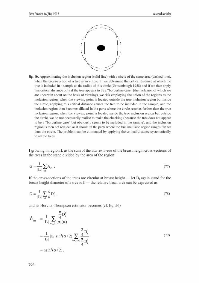
796


I growing in region L as the sum of the convex areas of the breast height cross-sections of the trees in the stand divided by the area of the region:

G = 1|L |

ACii∈I∑ .

(77)

If the cross-sections of the trees are circular at breast height — let Di again stand for the breast height diameter of a tree i∈I — the relative basal area can be expressed as

G = 1|L |

π4

Di2

i∈I∑ ,

(78)

and its Horvitz-Thompson estimator becomes (cf. Eq. 56)

G HT = 1|L |

π4

Di2


= 1|L |

|L | sin2(α / 2)

π4

Di2

π4

Di2i∈sQ (α )

∑

= nsin2(α / 2) ,

(79)

Fig. 16. Approximating the inclusion region (solid line) with a circle of the same area (dashed line), when the cross-section of a tree is an ellipse. If we determine the critical distance at which the tree is included in a sample as the radius of this circle (Grosenbaugh 1958) and if we then apply this critical distance only if the tree appears to be a “borderline case” (the inclusion of which we are uncertain about on the basis of viewing), we risk employing the union of the regions as the inclusion region: when the viewing point is located outside the true inclusion region but inside the circle, applying this critical distance causes the tree to be included in the sample, and the inclusion region then becomes dilated in the parts where the circle reaches farther than the true inclusion region; when the viewing point is located inside the true inclusion region but outside the circle, we do not necessarily realise to make the checking (because the tree does not appear to be a “borderline case” but obviously seems to be included in the sample), and the inclusion region is then not reduced as it should in the parts where the true inclusion region ranges farther than the circle. The problem can be eliminated by applying the critical distance systematically to all the trees.

797


where n is the number of trees in the sample sQ(α) obtained at point Q∈L with viewing angle α. Thus, an unbiased (with respect to the sampling design) estimate for the relative basal area is indeed attained by just counting the number of trees subtending the relascope angle — the fact perceived by Walter Bitterlich, at first only empirically (Bitterlich 1984)! The result follows from the fact that the inclusion area, and thereby also the inclusion probability, of each sampled tree i is proportional to πDi2/4 with 1/sin2(α/2) as the propor-tionality coefficient. (Note that ĜHT here is unitless, i.e., the cross-section areas and the area of the region L are assumed to be expressed in the same units; as mentioned before, the basal area factor sin2(α/2) is usually multiplied by 10 000 or 43 560 so as to express ĜHT in m2/ha or ft2/ac, respectively.)

If counting of trees is repeated at k randomly and independently selected viewing points Qj∈L, j=1, ..., k, G is unbiasedly estimated with the mean GHT of the k independent estima-tors ĜHTj; an unbiased estimator for the variance of GHT is given by

Var(G HT ) = 1k(k −1)

(G HTj−G HT )2

j=1

k

∑

= sin4(α / 2)k(k −1)

(n j − n)2

j=1

k

∑ ,

(80)

where n is the arithmetic mean of the numbers of trees nj counted at the k separate view-ing points.

If the convex closures of the breast height cross-sections of the trees are non-circular, the basal area estimator Ĝ=nsin2(α/2) is biased (when considered over the probability distribu-tion of all possible tree samples):

E(G) = sin2(α / 2)E(n)

= sin2(α / 2)E δ ii∈I∑ [sQ(α)]

⎧⎨⎩

⎫⎬⎭

= sin2(α / 2) π ii∈I∑ (α)

= sin2(α / 2)|Mi (α) |

|L |i∈I∑

= 1|L |

sin2

i∈I∑ (α / 2) |Mi (α) |

= 1|L |

sin2(α / 2)κ i (α)i∈I

∑ ACi

≡ 1|L |

Aii∈I∑ (α) .

(81)

Clearly, the bias of Ĝ owing to the non-circular shapes of tree cross-sections manifests itself in the deviation of Ãi(α) from ACi (Matérn 1956), that is, in the deviation of sin2(α/2)/κi(α) from 1. As sin2(α/2)/κi(α) was found to be larger or equal to 1 (Eq. 71) for all convex shapes, Ĝ tends to overestimate G systematically.

The inequalities proved by Matérn (1956) and introduced in the previous section (Eqs. 70 and 73) give bounds for the overestimating bias in Ĝ (originally, the inequalities were derived

798


expressly for the case of estimating relative basal area by relascope). The first inequality

Ai(α)− A0i ≤ A0i − ACi ⇔ ACi ≤ Ai(α) ≤ ACi + 2(A0i − ACi ) (82)

implies that, irrespective of the shape of a cross-section, Ã(α) be always greater or equal to the convex area of the cross-section, and that the error of Ã(α) never exceed double the iso-perimetric deficit. Accordingly, no matter what shapes breast height cross-sections assume,

G ≤ E(G) ≤ G + 2|L |

(A0i − ACi )i∈I∑ . (83)

The second inequality

A(α)− Eθ (A1) ≤ Eθ (A1)− AC⎡⎣ ⎤⎦ tan2(α / 2) (84)

shows that in practice — α being of the magnitude 1–2°, and tan2(α/2) thus 0.000076–0.00030 — Ã(α) becomes very close to the within-cross-section expectation Eθ(Â1) of the estimator based one random diameter. Accordingly,

E(G) ≈ 1|L |

Eθi∈I∑ (A1i ) , (85)

which implies that, regardless of the shapes of breast height cross-sections, the overesti-mating bias of the basal area estimator by relascope be approximately equal to the bias obtained by calipering all the trees in I in a random direction and applying the circle area formula (Matérn 1956).

Relative basal area may, of course, be estimated using diameter measurements, if they are available on the trees included in the Bitterlich sample. Then it is possible to apply different area estimators, say ÂX and ÂY, in the inclusion probability estimation versus the cross-section area estimation: the estimator with estimated inclusion probabilities becomes (cf. Eq. 67)

G = 1|L |

AYi


= 1|L |

AYi

AXi ⋅1

|L | sin2(α / 2)i∈sQ (α )∑

= sin2(α / 2)AYi

AXii∈sQ (α )∑ ,

(86)

and its expectation over the probability distribution of all possible tree samples is (cf. Eq. 69)

799


E(G) = AYii∈I∑ π i (α)

π i (α)

= AYii∈I∑

ACi ⋅1

κ i (α) |L |

AXi ⋅1

sin2(α / 2) |L |

= AYii∈I∑ ACi

AXi

⋅ sin2(α / 2)κ i (α)

.

(87)

For elliptical cross-sections, Grosenbaugh (1958) recommended using the geometric mean of Dmin and Dmax in the circle area formula for ÂY and the quadratic mean ditto for ÂX to minimise the bias. This is a most natural choice: the geometric mean in the circle area formula yields the true area AC of an ellipse, whereas the quadratic mean gives the largest overestimation and thus minimises the combined error sin2(α/2)/κ(α)·AC/ÂX.

4.2 Bitterlich Diameters: Diameters Measured Parallel or Perpendicular to Plot Radius Direction

When a tree to be investigated is selected by Bitterlich sampling, it is a common practice to measure its breast height diameter parallel or perpendicular to the plot radius, that is, parallel or perpendicular to the line segment from the viewing point to the assumed centre of gravity, or pith, of the breast height cross-section (Fig. 17). This diameter is then usually regarded as “random”, implying a correspondence to the diameter with the uniform direction distribution, which is the way in which “random diameter” is usually understood in colloquial language. Although practically sensible and seemingly sound, this practice involves a likely pitfall if the breast height cross-section of the tree is non-circular: Plot radius direction in Bitterlich sampling is a random variable the value of which depends on the outcome of the random experiment of placing the viewing point in the inclusion region. If the inclusion region of a stem deviates from a circle, the probability of a viewing point to be located in a certain direction when viewed from the tree pith varies according to the direction. In Fig. 17, for example, it is more probable to place the viewing point in the way that the plot radius direction becomes tQ than in the way that it becomes tR — simply because the line segment from the pith to the inclusion region boundary is longer through the point Q than through the point R. Accordingly, the distribution of the plot radius direction — and, in consequence, the distribution of the diameter measurement direction — is not uniform over [0, 2π) — or over [0, π), respectively — when viewed from the pith of the tree. In other words, contrary to the usual implicit assumption or belief, the diameter taken parallel or perpendicular to relascope plot radius direction does not correspond to a random diameter with the uniform direction distribution, if the cross-section of a tree is non-circular. In Fig. 17, for example, measuring diameters near D(tQ) is more probable than measuring diameters near D(tR) if the measurement practice is to take the diameter parallel to the plot radius, and less probable if the practice is to take the diameter perpendicular to the plot radius.

In the following, we first derive the direction distributions for these Bitterlich diameters, that is, for the diameters measured parallel or perpendicular to plot radius in Bitterlich sampling. Then we derive the expectations, variances and approximate variances of the area estimators similar to those dealt with in Section 3.3.2 but with Bitterlich diameters involved.

800


4.2.1 Direction Distributions of Bitterlich Diameters

The tree-specific probability distribution of the plot radius direction τ∈[0, 2π) is obtained from the inclusion region M(α) of the tree via geometrical probability. The density mass of τ between directions t1 and t2, t1<t2, is the probability that the viewing point is located in the sector of M(α) edged by the rays emanating from the tree pith in directions t1 and t2 (Fig. 18); since the viewing point is uniformly randomly located in the region of interest, the probability equals the area of the sector divided by the total area of M(α), that is,

Pr t1 ≤ τ ≤ t2; α{ } = |M(α)t1

t2 |

|M(α) | . (88)

The plot radius directions τ and τ+π result in the same diameter of the cross-section, and hence the probability that the direction ξ∈[0, π) of the diameter taken parallel to plot radius is between t1 and t2 is the sum of the probabilities of τ being between t1 and t2 or between t1+π and t2+π (Fig. 19), that is,

Pr t1 ≤ ξ ≤ t2; α{ } = Pr t1 ≤ τ ≤ t2; α{ } + Pr t1 + π ≤ τ ≤ t2 + π; α{ }

=|M(α)t1

t2 |

|M(α) |+

|M(α)t1+πt2+π |

|M(α) | .

(89)

Setting t1=0 and t2=t and restricting t∈[0, π), we obtain the cumulative distribution func-tion of ξ:

Fig. 17. In a tree with a non-circular breast height cross-section and, hence, with a non-circular inclu-sion region, measuring diameter in the plot radius direction does not result in a random diameter with the uniform direction distribution: here it is more probable to place the viewing point in the way that the plot radius direction becomes tQ than in the way that it becomes tR, because the line segment from the pith to the inclusion region boundary is longer through the point Q than through the point R; hence the diameter measurement is more likely to give a value D(tQ) than D(tR).

tQtR

D(tR)D(tQ)

Q

R

α

801


Fξ (t; α) = Pr ξ ≤ t; α{ } = Pr 0 ≤ ξ ≤ t; α{ } = Pr 0 ≤ τ ≤ t; α{ } + Pr π ≤ τ ≤ π + t; α{ } =

|M(α)0t |

|M(α) |+

|M(α)ππ+t |

|M(α) | .

(90)

Although the inclusion region boundary co-ordinates (Eq. C9 in Appendix C) or radii (Eq. 59) can straightforwardly be expressed as functionals of the support function p(·), the sector area of the inclusion region cannot, or at least this is rather troublesome; the difficulty lies in the determination of the integration limits (see Appendix D). Therefore, when computing the Bitterlich direction distribution, we resort to numerical integration.

The probability density function fξ(t; α)=Fξ′(t; α) may be approximated with

fξ (t; α) ≈Fξ (t + Δt; α)− Fξ (t; α)

Δt , (91)

where Δt is small (0.5°, for example). For the example shapes of Fig. 10, the approximated density functions with viewing angles 1°, 20° and 30° are shown in Fig. 20.

The direction distribution of the diameter taken perpendicular to plot radius in Bitterlich sampling is obtained from Fξ(t ; α) by a location shift of –π/2:

Fξ+π/2 (t; α) = Pr ξ + π / 2 ≤ t; α{ } = Pr ξ ≤ t − π / 2; α{ } = Fξ (t − π / 2; α) . (92)

M(α)M(α)

α

t1t2

t2t1

Fig. 18. Illustration of the probability distribution of the plot radius direction τ in Bitterlich sampling with α as the viewing angle: the density mass between directions t1 and t2 is the probability of the viewing point to be located in the hatched sector of the inclusion region M(α).

α

t1

D(t1)

t2D(t2)

M(α) t1t2

M(α) t1+πt2+π

Fig. 19. Illustration of the probability distribution of the direction ξ of the diameter measured parallel to plot radius direction in Bitterlich sampling with α as the viewing angle: the density mass between directions t1 and t2 is the probability of the viewing point to be located in either of the hatched sectors of the inclusion region M(α); D(t1) and D(t2) are the diameters in directions t1 and t2.

802


In the example shapes of Fig. 10, taking the Bitterlich diameter perpendicular to plot radius results in larger (or equal; shape F) values on average than taking it parallel to plot radius (Table 7), even though the differences are rather small (about 2.5 % in the ellipse A, less than 1 % in the other shapes). Compared to the diameters with the uniform direction distri-bution, the Bitterlich diameters parallel to plot radius are on average smaller in a majority

Fig. 20. (Approximated) probability density function fξ(ξ; α) of the direction ξ of the diameter taken parallel to plot radius in Bitterlich sampling for the six example shapes in Fig. 10. The distributions were determined with viewing angles α=1° (continuous line), α=20° (dotted line) and α=30° (dashed line). The positive x-axis, with respect to which the direction ξ is determined, runs horizontally through the centre of gravity of the shape; ξ increases anticlockwise. The horizontal line marks the density function 1/π of the uniform direction distribution.

Table 7. Means (μD(ξ), μD(ξ+π/2)) and variances (σD(ξ)2, σD(ξ+π/2)2) of Bitterlich diameters (D(ξ) taken parallel and D(ξ+π/2) taken perpendicular to plot radius direction) in relation to the same characteristics computed over the uniform direction distribution (μD, σD2) for five of the six example shapes in Fig. 10 (the orbiform B with constant diameter in every direction is omitted). The direction distributions of the Bitterlich diameters were determined with the viewing angles α=1° and α=30° (in parentheses).

ShapeA C D E F

μD(ξ)/μD (%) 98.79(98.95)

99.61(99.66)

99.70(99.71)

100.00(99.88)

100.39(100.19)

μD(ξ+π/2)/μD (%) 101.21(101.05)

100.39(100.34)

100.50(100.39)

100.65(100.44)

100.39(100.19)

σD(ξ)2/σD2 (%) 98.20(98.66)

99.32(99.44)

97.08(96.55)

99.76(99.80)

99.32(99.74)

σD(ξ+π/2)2/σD2 (%) 96.98(97.61)

99.32(99.44)

106.71(104.99)

99.11(99.52)

99.32(99.74)

0.0

0.1

0.2

0.3

0.4

A

f ξ(ξ

;α)

B0.0

0.1

0.2

0.3

0.4

C

f ξ(ξ

;α)

0 π 2 π0.0

0.1

0.2

0.3

0.4

D

f ξ(ξ

;α)

ξ0 π 2 π

E

ξ0 π 2 π

0.0

0.1

0.2

0.3

0.4

F

f ξ(ξ

;α)

ξ

803


Fig. 21. (Approximated) cumulative distribution functions of the Bitterlich diameters taken parallel (FD(ξ)(d) , black) or perpendicular (FD(ξ+π/2)(d), grey) to plot radius for the six example shapes in Fig. 10. The distributions were determined with viewing angles α=1° (continuous line) and α=30° (dashed line). For reference, the cumulative distribution function of the diameter with uniformly distributed direction within [0, π) is also shown (thin black line).

of the shapes, whereas the Bitterlich diameters perpendicular to plot radius are on average larger in all the shapes. Interestingly, in all the shapes but one, both types of the Bitterlich diameters seem to have a smaller variance than the diameters with the uniform direction distribution. The correlations between the Bitterlich diameters are the same (up to the third decimal) as the correlations between perpendicular diameters over the uniform direction distribution (Table 1; note that the shape B in this table is not the orbiform in Fig. 10 but the ellipse-like shape in Fig. 5).

From the direction distribution, we get the diameter distribution in a general manner: FD(ξ)(d) = Pr{D(ξ)≤d; α}, where Pr{D(ξ)≤d; α} is the probability mass of directions in which diameter is not larger than d. For the example shapes of Fig. 10, the Bitterlich diameter distributions are shown in Fig. 21.

4.2.2 Estimation of Cross-Section Area by Bitterlich Diameters and Circle Area Formula

As mentioned above, Bitterlich diameters (i.e., the diameters measured parallel or perpen-dicular to plot radius in Bitterlich sampling) are often used as if they were random diameters with the uniform direction distribution. As the direction distributions of the Bitterlich diam-eters are actually not uniform if the breast height cross-sections of trees are non-circular, we consider the cross-section area estimators similar to Â1–Â5 discussed in Section 3.3.2 but now involving Bitterlich diameters. The estimators are of the form

A = π4

D(⋅)2 ,

(93)

0.00

0.25

0.50

0.75

1.00A

F D(ξ

)(d),

F D(ξ

+π2)

(d) B

0.00

0.25

0.50

0.75

1.00C

F D(ξ

)(d),

F D(ξ

+π2)

(d)

d

0.00

0.25

0.50

0.75

1.00D

F D(ξ

)(d),

F D(ξ

+π2)

(d)

d

E

d

0.00

0.25

0.50

0.75

1.00F

F D(ξ

)(d),

F D(ξ

+π2)

(d)

804


where D(·) is1ξ. diameter D(ξ) taken parallel to plot radius direction, ξ~Fξ(ξ; α) (Â1ξ)2ξ. arithmetic mean of diameters D(ξ) and D(ξ+π/2) taken parallel and perpendicular to plot radius

direction (Â2ξ)3ξ. geometric mean of D(ξ) and D(ξ+π/2) (Â3ξ)4ξ. arithmetic mean of D(ξ) and an independent random diameter D(θ), ξ~Fξ(ξ; α), θ~Uniform(0, π)

(Â4ξ)5ξ. geometric mean of D(ξ) and D(θ) (Â5ξ)

Hardly surprisingly, the within-cross-section expectations, variances and variance approxi-mations of these estimators closely resemble those of the random estimators Â1–Â5 (Eqs. 22–26 and 30–37 in Section 3.3.2). If we denote the expectations of D(ξ) and D(ξ+π/2) taken over the distribution Fξ(ξ; α) by μD(ξ) and μD(ξ+π/2), the variances by σD(ξ)2 and σD(ξ+π/2)2, and the correlation by ρD(ξ)(π/2) (note that for brevity, the viewing angle α affecting the distribution is omitted in the notation) — and recall that μD and σD2 stand for the expecta-tion and the variance of D(θ) over the uniform distribution of θ — the expectations of the estimators become as follows:

E(A1ξ ) =π4µD(ξ )2 + π

4σD(ξ )2 ,

(94)

E(A2ξ ) = π4

µD(ξ ) + µD(ξ+π/2)

2⎛

⎝⎜

⎞

⎠⎟

2

+ π16

σD(ξ )2 + σD(ξ+π/2)

2 + 2σD(ξ ) σD(ξ+π/2) ρD(ξ )

π2

⎛⎝⎜

⎞⎠⎟

⎡

⎣⎢

⎤

⎦⎥ ,

(95)

E(A3ξ ) = π4µD(ξ ) µD(ξ+π/2) +

π4σD(ξ+π/2) σD(ξ ) ρD(ξ )

π2

⎛⎝⎜

⎞⎠⎟

, (96)

E(A4ξ ) = π4

µD(ξ ) + µD

2⎛

⎝⎜

⎞

⎠⎟

2

+ π16

σD(ξ )2 + σD

2( ) ,

(97)

and

E(A5ξ ) = π4µD(ξ ) µD .

(98)

Unlike with the expectations of the random estimators Â1–Â5, it is not easy to see whether these expectations overestimate or underestimate the convex area of a cross-section (because the relationship between πμD(ξ)2/4, or πμD(ξ+π/2)2/4, and AC is not straightforward to derive with no assumptions about cross-section shape; cf. Eq. 20 in Section 3.3.2). The exact variances are given by

Var(A1ξ ) = π2

16E[D(ξ)4]− µD(ξ )

2 + σD(ξ )2( )2{ } , (99)

805


Var(A2ξ ) = π2

161

16E[D(ξ)4]+ 1

16E D ξ + π

2⎛⎝⎜

⎞⎠⎟

4⎡

⎣⎢⎢

⎤

⎦⎥⎥+ 1

4E D(ξ)3D ξ + π

2⎛⎝⎜

⎞⎠⎟

⎡

⎣⎢

⎤

⎦⎥

⎧⎨⎪

⎩⎪

+ 14

E D(ξ)D ξ + π2

⎛⎝⎜

⎞⎠⎟

3⎡

⎣⎢⎢

⎤

⎦⎥⎥+ 3

8E D(ξ)2 D ξ + π

2⎛⎝⎜

⎞⎠⎟

2⎡

⎣⎢⎢

⎤

⎦⎥⎥

− 116

µD(ξ ) + µD(ξ+π/2)( )2+ σD(ξ )

2 + σD(ξ+π/2)2⎡

⎣⎢

+ 2σD(ξ ) σD(ξ+π/2) ρD(ξ )

π2

⎛⎝⎜

⎞⎠⎟⎤

⎦⎥

2 ⎫⎬⎪

⎭⎪ ,

(100)

Var(A3ξ ) = π2

16E D(ξ)2 D ξ + π

2⎛⎝⎜

⎞⎠⎟

2⎡

⎣⎢⎢

⎤

⎦⎥⎥

⎧⎨⎪

⎩⎪

− µD(ξ ) µD(ξ+π/2) + σD(ξ ) σD(ξ+π/2) ρD(ξ )

π2

⎛⎝⎜

⎞⎠⎟

⎡

⎣⎢

⎤

⎦⎥

2 ⎫⎬⎪

⎭⎪ ,

(101)

Var(A4ξ ) = π2

161

16E[D(ξ)4]+ 1

16E[D(θ)4]+ 1

4µDE[D(ξ)3]

⎧⎨⎩

+ 14µD(ξ )E[D(θ)3]+ 3

8µD(ξ )

2 + σD(ξ )2( ) µD

2 + σD2( )

− 116

µD(ξ ) + µD( )2+ σD(ξ )

2 + σD2⎡

⎣⎢⎤⎦⎥

2 ⎫⎬⎪

⎭⎪ ,

(102)

and

Var(A5ξ ) = π2

16µD(ξ )

2 + σD(ξ )2( ) µD

2 + σD2( )−µD(ξ )

2 µD2⎡

⎣⎤⎦ .

(103)

Finally, the variance approximations by the delta method become

Var(A1ξ ) =π2

4µD(ξ )2 σD(ξ )

2 , (104)

Var(A2ξ ) = π2

16µD(ξ ) + µD(ξ+π/2)

2⎛

⎝⎜

⎞

⎠⎟

2

σD(ξ )2 + σD(ξ+π/2)

2 + 2σD(ξ ) σD(ξ+π/2) ρD(ξ )

π2

⎛⎝⎜

⎞⎠⎟

⎡

⎣⎢

⎤

⎦⎥ ,

(105)

Var(A3ξ ) = π2

16µD(ξ )

2 σD(ξ+π/2)2 + µD(ξ+π/2)

2 σD(ξ )2⎡⎣

+ 2µD(ξ ) µD(ξ+π/2) σD(ξ ) σD(ξ+π/2) ρD(ξ )

π2

⎛⎝⎜

⎞⎠⎟⎤

⎦⎥ ,

(106)

806


Var(A4ξ ) = π2

16µD(ξ ) + µD

2⎛

⎝⎜

⎞

⎠⎟

2

σD(ξ )2 + σD

2( ) , (107)

and

Var(A5ξ ) = π2

16µD

2 σD(ξ )2 + µD(ξ )

2 σD2( ) .

(108)

Note that these variance approximations depend not only on the way of selecting the diam-eters — as with the estimators Â1–Â5 — but also on the type of mean employed in the estimator. For the estimator Â5ξ, the approximate variance is easily seen to underestimate the true variance, exactly as was the case with the estimator Â5 involving two diameters with the uniform direction distribution (cf. Eq. 38 in Section 3.3.2).

In practice, it is often more convenient to measure the (first) diameter perpendicular to plot radius than parallel to it. This practice results in three more area estimators of the form above to be considered: the modifications Â1ξ90, Â4ξ90 and Â5ξ90 of Â1ξ, Â4ξ and Â5ξ involving D(ξ+π/2) instead of D(ξ). The within-cross-section expectations and variances of the these estimators are obtained from those of Â1ξ, Â4ξ and Â5ξ by substituting the moments of D(ξ+π/2) for the moments of D(ξ).

In Tables 8 and 9, the expectations, variances and approximate variances of the estima-tors Â1ξ–Â5ξ, Â1ξ90, Â4ξ90 and Â5ξ90 are given for the example shapes in Fig. 10; the dis-tributions of ξ (and ξ+π/2) were determined with viewing angles 1° and 30°. None of the

Table 8. Expectations of the area estimators Â1ξ–Â5ξ, Â1ξ90, Â4ξ90 and Â5ξ90 (Eqs. 94–98) for the example shapes in Fig. 10 (the orbiform B with constant diameter in every direction is omitted, because in it all the estimators yield the same estimate, 1.042 times the true area), expressed in permille of true area. The distributions of the directions ξ and ξ+π/2 of the Bitterlich diameters were determined with the viewing angles α=1° and α=30° (in parentheses).

ShapeA C D E F

E(Â1ξ)/A (‰) 1000(1003)

1016(1017)

1014(1014)

1034(1031)

1040(1036)

E(Â2ξ)/A (‰) 1019(1019)

1022(1022)

1019(1018)

1037(1034)

1038(1034)

E(Â3ξ)/A (‰) 1013(1013)

1020(1020)

1018(1017)

1037(1034)

1040(1036)

E(Â4ξ)/A (‰) 1010(1011)

1019(1020)

1016(1016)

1032(1031)

1035(1033)

E(Â5ξ)/A (‰) 1006(1008)

1018(1019)

1014(1014)

1030(1029)

1034(1032)

E(Â1ξ90)/A (‰) 1050(1046)

1032(1031)

1030(1028)

1047(1043)

1040(1036)

E(Â4ξ90)/A (‰) 1034(1033)

1027(1026)

1024(1023)

1039(1037)

1035(1033)

E(Â5ξ90)/A (‰) 1031(1029)

1026(1025)

1022(1021)

1037(1035)

1034(1032)

807


estimators systematically underestimates the true area. As could be expected on the basis of diameter means (Table 7), the estimators involving the Bitterlich diameter parallel to plot radius (Â1ξ, Â4ξ and Â5ξ) yield smaller overestimating biases than those involving the Bitterlich diameter perpendicular to plot radius (Â1ξ90, Â4ξ90 and Â5ξ90). In all the shapes but F, the former estimators perform better, in terms of bias, than the estimators that were earlier found to be the best (Â0 and Â3; Table 8 vs. Table 2). As to the estimator variance, the type of the Bitterlich diameter involved in the estimator appears to have practically no effect (Table 9). The approximated variances virtually equal the true variances, which in turn hardly deviate from the variances obtained with the diameters with the uniform direc-tion distribution (Table 9 vs. Table 3).

Table 9. Square roots of the variances (Eqs. 99–103; Sd) and approximate variances (Eqs. 104–108; S d) of the area estimators Â1ξ–Â5ξ, Â1ξ90, Â4ξ90 and Â5ξ90 for the example shapes in Fig. 10 (the orbiform B with constant diameter in every direction is omitted, because in it the variances are identically zero), expressed in permille of true area. The distributions of the directions ξ and ξ+π/2 of the Bitterlich diameters were determined with the viewing angle α=1°; with α=30° the results were the same (up to a difference of 1 permille in a handful of cases).

Shape A C D E F

Sd(Â1ξ)/A (‰) 157 90 101 118 91S d(Â1ξ)/A (‰) 156 90 99 118 91Sd(Â2ξ)/A (‰) 4 0 45 83 91S d(Â2ξ)/A (‰) 4 0 45 83 91Sd(Â3ξ)/A (‰) 9 1 44 83 91S d(Â3ξ)/A (‰) 5 0 45 83 91Sd(Â4ξ)/A (‰) 112 64 71 83 64S d(Â4ξ)/A (‰) 112 64 70 83 64Sd(Â5ξ)/A (‰) 112 64 71 83 64S d(Â5ξ)/A (‰) 112 64 70 83 64Sd(Â1ξ90)/A (‰) 157 90 106 118 91S d(Â1ξ90)/A (‰) 159 90 104 118 91Sd(Â4ξ90)/A (‰) 112 64 73 83 64S d(Â4ξ90)/A (‰) 113 64 72 83 64Sd(Â5ξ90)/A (‰) 113 64 72 83 64S d(Â5ξ90)/A (‰) 113 64 72 83 64

808


5 Estimation of Stem VolumeAnalogously to the previous discussion on cross-section area estimation in Chapter 3, we now want to explore how diameter variation in non-circular cross-sections is reflected, via different diameter selection methods, to stem volume estimates or predictions. We consider three volume estimation methods — a volume equation, a theoretical general estimator (a definite integral of a cross-section area estimation function), and a definite integral of a non-parametric stem curve (a special case of the general estimator) — in which the input consists of tree height and diameters taken at two or more known (non-random) heights. Our interest is in the application of the volume estimation methods: we want to quantify how much of the estimation bias and error variance is attributable to uncertainty in the explanatory variables (diameters) and therefore seek to distinguish the error component due to diameter variation from the components related to other sources of uncertainty, such as model specification, parameter estimation and residual variation. The theoretical discussion in this chapter is a preliminary to the empirical part of the study, where the three types of volume estimators are investigated with real stems.

5.1 Practical Volume Estimator: Laasasenaho Volume Equation

The volume equations constructed by Laasasenaho (1982) are commonly used in Finland for predicting stem volume of standing trees from basic field measurements. We consider here the three-variable equation, with which the volumes of the sample trees are predicted for example in the Finnish national forest inventory (Tomppo et al. 1997). The model is of the form

V = β1D(⋅, 1.3)2 + β2D(⋅, 1.3)2 H + β3D(⋅, 1.3)3H + β4D(⋅, 1.3)2 H2

+ β5 D(⋅, 1.3)2 + D(⋅, 1.3)D(⋅, 6)+ D(⋅, 6)2⎡⎣ ⎤⎦ + β6D(⋅, 6)2(H − 6) + εL , (109)

where V denotes the stem volume, D(·, 1.3) is the breast height diameter, D(·, 6) is the upper diameter taken at the height of 6 m, H stands for the stem height, and εL is a random error with certain properties discussed in more detail below. As indicated by the denotations D(·, 1.3) and D(·, 6), the diameters in the model have not been explicitly specified (in which direction they should be measured, whether they should be computed as a mean of two or more diameters etc.). We fix them here as those yielding the true cross-section areas when substituted in the circle area formula, denoted by DA(1.3) and DA(6):

V = β1DA (1.3)2 + β2DA (1.3)2 H + β3DA (1.3)3H + β4DA (1.3)2 H2

+ β5 DA (1.3)2 + DA (1.3)DA (6)+ DA (6)2⎡⎣ ⎤⎦ + β6DA (6)2(H − 6) + εL . (110)

This specification, albeit not very feasible in practice, is well motivated by the geometrical background of the model (see Laasasenaho 1982, p. 35–39) and also serves our purpose of extracting the effect of non-circularity on prediction error.

The model was constructed on the basis of data on 5053 trees sampled from all over Finland (Laasasenaho 1982), and hence it may be considered to express the dependence of stem volume on diameters and height in the Finnish tree population, with different parameter values β1, ..., β6 for different species. This population is finite but so large that sampling from it more or less corresponds to sampling from a theoretical infinite population.

809


Randomness arises from choosing a tree in the population, and both the response variable and the explanatory variables may be regarded as random variables, the joint distribution of which is generated by repeated independent samplings from the population. As usual with random explanatory variables, the distributional properties of the error term εL are defined conditional on the explanatory variables: given any possible combination of values of DA(1.3), DA(6) and H in the population, εL is assumed to have zero expectation and vari-ance proportional to DA(1.3)4H2 (Laasasenaho 1982, p. 36 and p. 43–44); further, εL’s of separate trees are assumed to be independent. From the zero conditional expectation of εL it follows that the expectation of εL is zero also marginally, that is, over the joint distribution of DA(1.3), DA(6) and H in the population.

We assume the equation to express the relation correctly, that is, the functional form as well as the values of the coefficients β1, ..., β6 to be true in the population of our interest, and wish to use it to predict the volume of a (randomly selected) tree in this population, when the two diameters and the height of the tree are known. The best predictor is the model without the error term, that is, the conditional expectation of the volume:

VL = E[V | DA (1.3), DA (6), H]

= β1DA (1.3)2 + β2DA (1.3)2 H + β3DA (1.3)3H + β4DA (1.3)2 H2

+β5 DA (1.3)2 + DA (1.3)DA (6)+ DA (6)2⎡⎣ ⎤⎦ + β6DA (6)2(H − 6) .

(111)

As there is no estimation error in the parameter values, the prediction error V–VL naturally equals the random error εL and follows the assumptions made on εL (i.e., E[V–VL | DA(1.3), DA(6), H]= E[V–VL]=0 and Var[V–VL | DA(1.3), DA(6), H] ∝ DA(1.3)4H2).

If we then view volume prediction within the tree of interest, the setting becomes very similar to that of cross-section area estimation in Chapter 3: volume is now a fixed property of the tree that we estimate by a fixed estimator VL, and the estimation error V–VL becomes a non-random scalar (a realisation of εL). We adopt this within-tree view for a while to deal with volume predictors involving random diameters.

Consider estimating the stem volume of the tree by using some diameters other than DA(1.3) and DA(6), measured without error at the heights of 1.3 m and 6 m. Denote these diameters by D(θ, 1.3) and D(θ, 6), θ referring here to the diameter direction selection method in general. As the height H is known, the estimator can now be written as a func-tion of the diameters only:

VL(θ) = c1D(θ,1.3)2 + c2D(θ,1.3)3 + c3D(θ,1.3)D(θ,6) + c4D(θ,6)2 , (112)

where c1=β1+β2H+β4H2+β5, c2=β3H, c3=β5, and c4=β5+β6(H–6). If the selection of D(θ, 1.3) and D(θ, 6) involves randomness, the estimator becomes a random variable, the within-tree distribution of which is determined by the diameter selection method and the shape of the cross-sections at the heights of 1.3 m and 6 m. As with random area estimators (Section 3.3.2), the random volume estimator can be thought to consist of a systematic part and a stochastic part — the within-tree expectation over the diameter direction distribution and a random sampling error with zero expectation over the same distribution:

VL(θ) = Eθ[VL(θ)]+ νL(θ) . (113)

As the estimator is a linear combination of the second and third powers of diameters and their cross-product, its within-tree expectation and variance are obtained by means of the

810


corresponding diameter moments and product moments taken over the diameter direction distribution:

Eθ[VL(θ)] = c1Eθ[D(θ,1.3)2] + c2Eθ[D(θ,1.3)3]

+ c3Eθ[D(θ,1.3)D(θ,6)] + c4Eθ[D(θ,6)2] , (114)

and

Varθ[νL(θ)] = Varθ[VL(θ)]

= Eθ[VL(θ)2] − Eθ[VL(θ)]{ }2

= c22Eθ[D(θ,1.3)6] + 2c1c2Eθ[D(θ,1.3)5] + c1

2Eθ[D(θ,1.3)4]

+ 2c2c3Eθ[D(θ,1.3)4 D(θ,6)] + 2c2c4Eθ[D(θ,1.3)3D(θ,6)2]

+ 2c1c3Eθ[D(θ,1.3)3D(θ,6)] + (c32 + 2c1c4 )Eθ[D(θ,1.3)2 D(θ,6)2]

+ 2c3c4Eθ[D(θ,1.3)D(θ,6)3] + c42Eθ[D(θ,6)4]

− Eθ[VL(θ)]{ }2 .

(115)

Each diameter selection method can in principle be applied either dependently or indepen-dently at the two observation heights within the stem: in the former, the diameter direction is selected at breast height, and the upper diameter is then measured in the same direction; in the latter, the diameter directions at the two heights are selected independently. In Bitterlich sampling, however, the idea of selecting diameters parallel or perpendicular to plot radius independently at the two heights is unfeasible (the plot radius direction is determined only once, from one viewing point at the breast height level); therefore, only dependent selection can be considered with the methods involving Bitterlich diameters. In the above expressions of within-tree expectation and variance, independent and dependent selection differ from each other only in terms of the product moments E[D(θ, 1.3)kD(θ, 6)p], k, p∈Q+, which in the independent case reduce to the products of moments E[D(θ, 1.3)k]E[D(θ, 6)p]. In Appendices E and F, more elaborate method-specific versions of the above general expres-sions of within-tree expectation and variance are given for the diameter selection methods involving randomness and considered previously in area estimation (methods 1–5 involving the uniform direction distribution, see Section 3.3.2; methods 1ξ–5ξ, 1ξ90, 4ξ90 and 5ξ90 involving Bitterlich diameter direction distribution, see Section 4.2.2).

No matter if we are viewing volume determination at the within-tree level (volume esti-mation) or at the population level (volume prediction), the volume error V–VL(θ) may be thought to consist of two components — the error term inherent in the model (the differ-ence between the true volume V and the best predictor/estimator VL) and the error due to diameter selection (the difference between the best predictor/estimator VL and the predic-tor/estimator VL(θ) obtained with the particular diameter selection method θ); further, the error due to diameter selection can be divided into two components — the within-tree bias VL–Eθ[VL(θ)] taken with respect to the best predictor/estimator and a random sampling error νL(θ):

811


V − VL(θ) = (V − VL ) + VL − VL(θ)⎡⎣ ⎤⎦

= εL + VL − Eθ[VL(θ)]+ νL(θ){ }{ } = εL + VL − Eθ[VL(θ)]{ } − νL(θ) .

(116)

At the within-tree level (conditional on the selected tree), only the within-tree diameter sam-pling error νL(θ) is a random variable (with zero expectation, variance Varθ[νL(θ)]=Var[VL(θ)], and the distribution determined by the diameter sampling method and the shapes of the cross-sections at 1.3 m and 6 m), whereas the model error εL and the within-tree systematic error due to diameter selection VL–Eθ[VL(θ)] are non-random scalars and may in princi-ple be compared to each other. At the population level, however, all the prediction error components are random variables. Yet we have only made assumptions on the model error εL. In any event, the prediction bias E[V–VL(θ)] at the population level consists of only the between-trees expectation E{VL–Eθ[VL(θ)]} of the within-tree bias due to diameter selection, as E(εL)=0 by assumption and E[νL(θ)]=Etree{Eθ[νL(θ) | tree]}=0. The prediction error variance Var[V–VL(θ)], in turn, comprises the variances of all the error components (εL, VL–Eθ[VL(θ)] and νL(θ)) taken over their marginal distributions as well as double the pairwise covariances computed over their joint distribution.

Above we assumed the model (Eq. 110) to be true. If, however, the true values for the parameters β1, ..., β6 were unknown and we had to use estimates obtained from any sub-population, the prediction error V–VL would also contain a component due to the parameter estimation error (see e.g. Fox 1984; cf. Gregoire and Williams 1992): even if the parameters were unbiasedly estimated, the prediction bias at the population level would be zero only when averaged over (infinitely many) repeated parameter estimations; furthermore, the prediction error variance would increase by a non-zero term depending on the variances and covariances of the parameter estimates and the values of the predicting variables.

5.2 GeneralVolumeEstimator:DefiniteIntegralofCross-SectionAreaEstimationFunction

The true volume of a stem is attained as a definite integral of the cross-section area function — a continuous and bounded function A:[0, H]→[0, ∞) expressing how the cross-section area perpendicular to the vertical stem axis changes along the position in the axis:

V = A0

H

∫ (h)dh . (117)

Substituting for the area function an estimate Â(h; θ) (where θ just generally refers to the features of the function distinguishing it from other area estimation functions) results in a volume estimator of the form

VG (θ) = A0

H

∫ (h; θ)dh . (118)

Estimators of this kind, where no presumptions (besides boundedness) are necessarily made on Â(h; θ), are here referred to as general volume estimators. (We can not require continuity of Â(h; θ), if we want to allow it to be constructed from random diameters selected independently of each other at all the heights h∈[0, H]; see the discussion below.)

812


Unlike with the volume equation earlier, we now choose to disregard the tree population level — although many population level models for the area estimation function (cross-section area taper models) are to be found in the literature (for a statistical consideration of prediction by such models, without uncertainty in the explanatory variables, refer e.g. to Gregoire et al. 2000). Instead, we adopt the within-tree view and simply regard the stem volume as a fixed property of our tree of interest, which we then want to estimate by means of an estimated cross-section area function (typically derived from either fixed or random diameters taken at predetermined heights) and the tree height. Within-tree randomness in the volume estimator then arises from randomness in the estimated area function (typically stemming from the use of random diameters in the construction of the function).

If Â(h; θ) is a random function (θ now referring to the source of randomness, typically the selection method of random diameter directions), it can equivalently be regarded as a continuous parameter stochastic process {Â(h; θ), h∈[0, H]} within the tree (cf. Rao 1979, p. 2). We are interested in the definite integrals of this process (to get the volume estimator) and of its transformation, the area estimation error process {Â(h; θ)–A(h), h∈[0, H]} (to get the volume estimation error). The definite integrals are well-defined (as limits, in the sense of convergence in mean square, of the sequences of approximating sums (Riemann sums) over [0, H] or any of its sub-intervals), if the processes satisfy the following sufficient (but not necessary!) conditions (Parzen 1962, p. 78–79): First, the processes should have finite second moments. In our case, this is necessarily true, as both {Â(h; θ)} and {A(h)} are bounded. Second, the processes should have continuous mean and covariance functions μÂ(h; θ)=Eθ[Â(h; θ)], μΔÂ(h; θ)=Eθ[Â(h; θ)–A(h)] and γÂ(h, k; θ)=Covθ[Â(h; θ), Â(k; θ)]= Covθ[Â(h; θ)–A(h), Â(k; θ)–A(k)]=γΔÂ(h, k; θ). Although Â(h; θ) based on diameters taken in independent random directions at each height is not necessarily continuous, its mean and covariance functions are, as they consist of diameter means, variances and covariances that change with height within a stem smoothly, with no discontinuity. Hence, we can assume that our processes fulfil also the second condition.

For processes satisfying the above conditions, the expectation and variance of their definite integrals are given by the definite integrals of the mean and covariance functions (Parzen 1962, p. 79). Accordingly, for the area estimation process and the area estimation error process

Eθ[VG (θ)] = Eθ A0

H

∫ (h; θ)dh⎡

⎣⎢⎢

⎤

⎦⎥⎥

= µA

0

H

∫ (h; θ)dh ,

(119)

Eθ VG (θ)− V⎡⎣ ⎤⎦ = Eθ A0

H

∫ (h; θ)dh − A0

H

∫ (h)dh⎡

⎣⎢⎢

⎤

⎦⎥⎥

= Eθ A(h; θ)− A(h)⎡⎣ ⎤⎦dh0

H

∫⎧⎨⎪

⎩⎪

⎫⎬⎪

⎭⎪

= µΔA

0

H

∫ (h; θ)dh ,

(120)

and

813


Varθ[VG (θ)] = Varθ A0

H

∫ (h; θ)dh⎡

⎣⎢⎢

⎤

⎦⎥⎥

= γA

0

H

∫0

H

∫ (h,k; θ)dhdk

= γΔA

0

H

∫0

H

∫ (h,k; θ)dhdk

= Varθ A(h; θ)− A(h)⎡⎣ ⎤⎦dh0

H

∫⎧⎨⎪

⎩⎪

⎫⎬⎪

⎭⎪

= Varθ VG (θ)− V⎡⎣ ⎤⎦ .

(121)

In other words, the within-tree expectation and variance of a general volume estimator are attained by integrating the mean and covariance functions of the underlying area estima-tion process; further, the within-tree bias is obtained by integrating the mean function of the area estimation error process.

A theoretical upper bound for the within-tree variance of a general volume estimator is attained by assuming that the elements of the area estimation process are fully positively correlated, that is, by assuming that ρÂ(h, k)=Corrθ[Â(h; θ), Â(k; θ)]=1 for all h and k in [0, H]. In this case, the covariance function of the area estimation process becomes

γA

(h,k; θ) = σA2 (h; θ)σ

A2 (k; θ) , (122)

where σÂ2:[0, H]→[0, ∞), σÂ2(h; θ)=Varθ[Â(h; θ)] is the variance function of the area estimation process, and this yields

Varθ[VG (θ) | ρA (h, k) = 1] = σA2 (h; θ)

0

H

∫ dh⎡

⎣⎢⎢

⎤

⎦⎥⎥

2

(123)

as the volume estimator variance.An area estimation process with uncorrelated elements makes another interesting spe-

cial case. Envisage a process where the correlation between elements Â(h; θ) and Â(k; θ) decreases with an increasing distance between h and k, finally to vanish with distances larger than some threshold value. It can be shown that as the threshold distance is diminished toward zero, that is, as the correlations between elements nearer and nearer each other are made vanish, the variance of the corresponding volume estimator (the variance of the integral of the process) tends to zero. The “limiting process” with mutually uncorrelated elements, that is, with Corrθ[Â(h; θ), Â(k; θ)]=0 for all h≠k in [0, H], is necessarily discontinuous and possesses a discontinuous covariance function with non-zero values (σÂ2(h; θ)) only within the diagonal line k=h. In our tree stem context, this kind of process would arise, for example, if Â(h; θ) was based on diameters taken in independent random directions at all the heights h∈[0, H]. In practice, however, this process has no natural construction: we may well generate individual process elements (area estimators) that are uncorrelated with each other — by independent selection of random diameter directions, for example — but only sparsely, at a finite number of observation heights, not at the infinite number of all possible heights. To obtain a volume estimate, we need to know the values of the area estimation process at all the heights h∈[0, H], and these we attain by assuming continuity — and, thus, some degree of correlation — between our finite number of observed values. Ergo, from

814


a practical point of view, an area estimation process with uncorrelated elements is just an abstraction that cannot indeed exist in our tree stem context.

A natural practice would be to assume a model for the area estimation function Â(h; θ) in a tree and derive from it (empirical) approximations of μΔÂ(h; θ), γÂ(h, k; θ), and σÂ2(h; θ) (cf. Section 5.3). In the empirical part of this study, however, we will construct crude approximations of μΔÂ(h; θ), γÂ(h, k; θ), and σÂ2(h; θ) in a data-driven manner, without an explicit model for Â(h; θ): We will consider area estimation processes where the area estimator at each height is one of the area estimators discussed in Sections 3.3 and 4.2.2. For each process, we will approximate μΔÂ(h; θ), γÂ(h, k; θ), and σÂ2(h; θ) by just interpolating between discrete observations of the process mean, covariance and vari-ance in the stem — between the elements of a vector containing the within-cross-section biases (Eθ[Â(h; θ)]–A(h))h∈H, a matrix containing the between-cross-sections covariances (Covθ[Â(h; θ), Â(k; θ)])h, k∈H, and a vector containing the within-cross-section variances (Varθ[Â(h; θ)])h∈H of the area estimator observed at fixed heights H={h(1), h(2), ..., h(m)} in the stem. Evidently, a unique area estimation function Â(h; θ) that would exactly cor-respond to the obtained μΔÂ(h; θ), γÂ(h, k; θ), and σÂ2(h; θ) may not even exist, whereas there are likely to be many whose mean, covariance and variance functions are reasonably adequately approximated by the obtained functions.

5.3 VolumeEstimatorBasedonNon-ParametricStemCurve:DefiniteIntegralofInterpolatingCubicSplines

Irrespective of the variation in cross-section shape in the stem, the area estimation func-tion in the integral expression of stem volume (Eq. 117) can equivalently be written as A(h)=πDA(h)2/4, where DA:[0, H]→[0, ∞) is a continuous and bounded function express-ing the true area diameter (i.e., the diameter that yields the true cross-section area when substituted in the circle area formula) at height h. The true volume of a stem is thus given by

V = π4

DA0

H

∫ (h)2dh , (124)

and DA(·) is referred to as the true stem curve.A plethora of methods have been suggested to predict or estimate DA(·) (see Sterba 1980,

and, for instance, Laasasenaho 1982 and Lappi 1986). In this study, we consider cubic spline interpolation between diameters measured at several non-random heights in a stem: the stem curve is composed of piecewise defined 4th order (3rd degree) polynomials of height, one polynomial for each interval between two adjacent measurement heights; each polynomial is required to pass through the endpoints of its domain (the observed (height, diameter)-points), and the smoothness of the whole interpolant is ensured by requiring its first and second derivatives to be continuous over the whole domain [0, H], that is, also in every point of junction of the polynomials. The number of diameter measurements permit-ting, this approach has quite commonly been used in Finland to estimate stem volume for research purposes (see e.g. Laasasenaho 1982, Lappi 1986, Ojansuu 1993, and Mäkinen et al. 2002).

We are now to examine how diameter selection within cross-sections at predetermined heights affects volume estimation by cubic-spline-interpolated stem curves. As with the family of general volume estimators in Section 5.2, the members of which these estimators patently are, we adopt the within-tree view: we regard the stem volume as a fixed property

815


of a tree and randomness in volume estimation as arising from diameter selection within the cross-sections at the non-random observation heights.

We omit discussing the potential difficulties in the practical use of interpolating cubic splines — how to determine the initial values optimally and how to avoid non-monotonicity or oscillation, for example, which aspirations manifest themselves in the empirical rules about the required number and distribution (along the vertical axis) of the measurement heights (see Lahtinen and Laasasenaho 1979, and Lahtinen 1988) — but simply assume that we have at our disposal an adequate set of error-free diameter measurements from an adequate set of fixed heights.

Let us denote by S3(h; D, H) the interpolating cubic spline based on a vector of diameters D=(D(h(1)), D(h(2)), ..., D(h(m))) taken (by some selection method) at predetermined heights H=(h(1), h(2), ..., h(m)). Presumably the best stem volume estimate is given by the stem curve obtained from the observed true area diameters DA=(DA(h(1)), DA(h(2)), ..., DA(h(m))):

VS =π4

S30

H

∫ (h; DA , H)2dh . (125)

The estimation error in VS now results from the interpolation procedure, that is, from the deviation of the estimated stem curve S3(· ; DA, H) from the true stem curve DA(·) in other points than those included in DA.

In practice, not knowing the cross-section areas at the observation heights, we have to do with other diameters than the true area ones; let us denote a vector of such diameters by D(θ)=(D(θ, h(1)), D(θ, h(2)), ..., D(θ, h(m))), θ referring to the diameter selection method. If the selection method involves randomness, D(θ) is a random vector and the interpolated stem curve S3[h; D(θ), H] becomes a random function. Naturally, the volume estimator

VS(θ) =π4S3

0

H

∫ [h; D(θ), H]2dh (126)

is then also a random variable. Following the theory presented in Section 5.2 for the family of general volume estimators, we could now attempt to estimate the within-tree expectation and variance of this estimator by integrating the mean and covariance functions μÂ(h; θ) and γÂ(h, k; θ) of the area estimation process {Â(h; θ), h∈[0, H]}={πS3[h; D(θ), H]2/4, h∈[0, H]} in a stem. However, the functions appear to be difficult to derive analytically, as the coefficients determining the values of S3[h; D(θ), H] between any two elements of H (the observation heights) are nonlinear functions of the elements of D(θ). Thus, instead of pursuing the mean and covariance functions of {πS3[h; D(θ), H]2/4, h∈[0, H]}, we con-sider estimating the within-tree expectation and variance of VS(θ) by means of a number of repeated estimations (realisations of the volume estimator).

In principle, to obtain a realisation VS(θi) of the volume estimator, we draw a vector of diameter directions θi=(θi(h(1)), θi(h(2)), ..., θi(h(m))) from the joint distribution of the diameter directions at the fixed observation heights (the distribution is specific to the diameter selection method), measure the corresponding diameters D(θi)=(D[θi(h(1)), h(1)], D[θi(h(2)), h(2)], ..., D[θi(h(m)), h(m)]) at different heights, interpolate between the diameters, and integrate the square of the resulting stem curve realisation S3[h; D(θi), H].

If the diameter selection method involves such dependence between the diameters that the measurement direction chosen at one height determines the measurement directions at the other heights, that is, if all the elements of the direction vector θi are transformations of the direction θi(h(k)) associated to one observation height h(k)∈H, the multidimensional direction distribution reduces into a one-dimensional one. This is the case, for example,

816


when the diameters at different heights are measured in the same direction decided upon at breast height (cf. the dependent selection in Section 5.1). The expectation and variance of the volume estimator are then obtained by numerical integration over the one-dimensional direction distribution: we select values for θi(h(k)), i=1, ..., n, equidistantly within [0, π), estimate from the direction distribution a weight wi associated to each θi(h(k)) as the prob-ability of selecting a direction not farther than half the equi-interval from θi(h(k)), derive from each θi(h(k)) the direction vector θi and determine the corresponding diameter vector D(θi), compute the volume estimator realisation VS(θi) associated to each D(θi), and then estimate the within-tree expectation and variance of the volume estimator as the weighted mean and variance of the n realisations:

Eθ[VS(θ)] = wiVS(θi )i=1

n

∑ wii=1

n

∑

= wi

π4

S30

H

∫ [h; D(θi ), H]2dh⎧⎨⎪

⎩⎪

⎫⎬⎪

⎭⎪i=1

n

∑ wii=1

n

∑ ,

(127)

and

Varθ[VS(θ)] = wi VS(θi )− Eθ[VS(θ)]{ }2

i=1

n

∑ wii=1

n

∑ . (128)

Naturally, if the one-dimensional direction distribution is uniform, all the weights wi are equal and the expectation and variance can be estimated with simple (non-weighted) mean and variance.

If the diameter selection method involves no simplifying dependence between the diameters at the different heights, we resort to Monte Carlo integration, where the direc-tion vectors θi, i=1, ..., n, are sampled independently from the multidimensional direction distribution. In this case, the within-tree expectation and variance of the volume estimator are then estimated simply with the mean and variance of the n realisations (Robert and Casella 2000):

Eθ[VS(θ)] = 1n

VSi=1

n

∑ (θi ) , (129)

and

Varθ[VS(θ)] = 1n

VS(θi )− Eθ[VS(θ)]{ }2

i=1

n

∑ . (130)

Interestingly, there is a straightforward connection between these estimates (Eqs. 127–130) and the estimates obtained by integrating the mean and covariance functions μÂ(h; θ) and γÂ(h, k; θ) of the area estimation process {Â(h; θ), h∈[0, H]}={πS3[h; D(θ), H]2/4, h∈[0, H]} (Eqs. 119 and 121), namely, the above estimates imply certain approximations for μÂ(h; θ) and γÂ(h, k; θ): Estimating the expectation of VS(θ) as the (weighted) mean of the volume estimates computed from a sample of diameter vectors (Eqs. 127 and 129) corresponds to approximating μÂ(h; θ) at each h by the (weighted) mean of a sample of area estimation function realisations (stem curve realisations) Â(h; θi)=πS3[h; D(θi), H]2/4, i=1, ..., n:

817


Eθ[VS(θ)] = wii=1

n

∑ VS(θi ) w ii=1

n

∑

= wii=1

n

∑ A0

H

∫ (h; θi )dh⎡

⎣⎢⎢

⎤

⎦⎥⎥

wii=1

n

∑

= wii=1

n

∑ A(h; θi ) w ii=1

n

∑⎡

⎣⎢

⎤

⎦⎥

0

H

∫ dh

≡ µA

0

H

∫ (h)dh

≈ µA

0

H

∫ (h)dh

= Eθ[VG (θ)] .

(131)

Similarly, estimating the variance of VS(θ) as the (weighted) variance of the volume estimates computed from a sample of diameter vectors (Eqs. 128 and 130) corresponds to approximating γÂ(h, k; θ) by the (weighted) covariance computed at each (h, k) from a sample of area estimation function realisations (stem curve realisations):

Varθ[VS(θ)] = wii=1

n

∑ VS(θi )− Eθ[VS(θ)]{ }2wi

i=1

n

∑

= wi A0

H

∫ (h; θi )dh − µA

0

H

∫ (h)dh⎧⎨⎪

⎩⎪

⎫⎬⎪

⎭⎪

2

i=1

n

∑ wii=1

n

∑

= wi A(h; θi )− µA(h)⎡⎣ ⎤⎦

0

H

∫ dh⎧⎨⎪

⎩⎪

⎫⎬⎪

⎭⎪

2

i=1

n

∑ wii=1

n

∑

= wii=1

n

∑ A(h; θi )− µA(h)⎡⎣ ⎤⎦ A(k; θi )− µA

(k)⎡⎣ ⎤⎦dhdk0

H

∫0

H

∫⎧⎨⎪

⎩⎪

⎫⎬⎪

⎭⎪wi

i=1

n

∑

= wii=1

n

∑ A(h; θi )− µA(h)⎡⎣ ⎤⎦ A(k; θi )− µA

(k)⎡⎣ ⎤⎦ wii=1

n

∑⎧⎨⎩

⎫⎬⎭0

H

∫0

H

∫ dhdk

≡ γA

0

H

∫0

H

∫ (h, k)dhdk

≈ γA

0

H

∫0

H

∫ (h, k)dhdk

= Varθ[VG (θ)] .

(132)

In other words, at each point (h, k), the definite integrals in μÂ(h; θ)=Eθ[Â(h; θ)] and γÂ(h, k; θ)=Covθ[Â(h; θ), Â(k; θ)] taken over the multidimensional direction distribution (the joint distribution of the diameter directions at the fixed observation heights) are approximated with sums, sums of the squares or sums of the products of n area estimates Â(h; θi)= πS3[h; D(θi), H]2/4 based on n direction vector realisations θi drawn from the distribution.

818


In Section 5.2 we discovered that as the elements of a stochastic area estimation process become uncorrelated, the within-tree variance of the corresponding generalised volume estimator becomes zero; moreover, we noted that such a discontinuous process is an abstrac-tion that cannot really be generated in a tree stem context (by e.g. independent diameter selection at a finite number of observation heights). Evidently, cubic spline interpolation between uncorrelated (independently selected) random diameters at the observation heights does not result in a volume estimator with zero variance, often quite the contrary: the area estimators at the observation heights are of course mutually independent, but the interpo-lated curve imposes continuity and induces short-distance dependence (non-zero covariance between heights close to each other) for the area estimators at the heights in between (via spline coefficients involving common diameters), thus making the integral of the resulting covariance function deviate from zero.

As with the volume equation in Section 5.1, the volume estimation error V–VS(θ) can be divided into the two distinct additive components — the error V–VS=εS inherent in the best estimator VS and the error VS–VS(θ) attributable to diameter selection by method θ — the latter of which further consists of two components — the within-tree bias VS–Eθ[VS(θ)] with respect to the best estimator and a random sampling error νS(θ):

V − VS(θ) = (V − VS ) + [ VS − VS(θ)]

= εS + VS − Eθ[VS(θ)]+ νS(θ){ }{ } = εS + VS − Eθ[VS(θ)]{ } − νS(θ) .

(133)

At the within-tree level only νS(θ) is a random variable (with zero expectation and variance Varθ[νS(θ)]=Varθ[VS(θ)]), whereas at the population level all the estimation error compo-nents are random variables. The interpretation of the error εS contained in the best non-parametric estimator VS, however, does not straightforwardly parallel that of the model error term εL of the parametric volume equation: In our “model” V=VS+εS, we have incorporated no distributional assumptions on εS that would then have governed the estimation of VS. In particular, the population expectation of εS may well deviate from zero, whereupon the estimation bias E[V–VS(θ)] at the population level may involve not only the between-trees expectation E{VS–Eθ[VS(θ)]} of the within-tree bias due to diameter selection but also the population expectation E(εS).

819


6 MaterialThe material of the study consists of a small subset of the sample trees felled and measured in 1991 for the nationwide tree quality investigation (VAPU) of the Finnish Forest Research Institute. In the investigation, the forest stand population of Finland was divided into the strata of Scots pine, Norway spruce and silver/pubescent birch dominated stands, in each of which the following four-stage sampling was then performed: First, a subset of 20 clus-ters were systematically chosen among the clusters of plots placed systematically all over Finland in the 7th National Forest Inventory (for the sampling design of the inventory, see Kuusela and Salminen 1980 and Kuusela et al. 1986). Second, two plots among the total of 28 in each cluster were systematically selected for tree sampling. Third, 20 tally trees were picked in each selected plot (first the four trees growing closest to the plot centre, and then the 16 dominant or codominant trees next closest to the centre); the trees had to fulfill certain selection criteria (living trees of species Scots pine, Norway spruce or silver/pubescent birch with no visible biotic or abiotic defects and with breast height diameter not less than 7 cm). Fourth, six sample trees to be felled in each plot were randomly chosen among the 20 tally trees (three trees among all the tally trees and three trees among the tally trees of dominant species and dominant crown class). Among the sample trees taken from the stratum of the Scots pine dominated stands, a judgement sample was then drawn for this study, resulting in a total of 81 trees from 16 plots in 11 clusters (Fig. 22, Table 10).

The geographical distribution of the selected trees was somewhat uneven in both the north–south and east–west directions, in which some noteworthy variation in stem form is known to occur in Finland (e.g. Lappi 1986): in Southern Finland (Fig. 22) 26 stems were measured on six plots, while in Northern Finland 55 stems were taken on ten plots; further, east of the centre meridian 27° of the Finnish national uniform co-ordinate system, only 14 stems were measured on three plots, whereas west of it 67 stems were taken on 13 plots.

All the 16 plots were located in naturally regenerated one-storey stands; while ten of these were pure Scots pine stands, four contained some Norwegian spruce mixture and two silver/pubescent birch mixture. A majority of the stands grew on mineral soil (Table 10); of

Fig. 22. Locations of the 11 clusters of plots in which the 81 trees investigated in this study were felled (degrees east longitude and north latitude). The line across the country marks the division between Southern Finland and Northern Finland. For the information of the plots in the clusters, see Table 10.

820


the seven stands located in peatland, five were drained — in two of these the drainage had been completed so recently that the drainage effect could not yet be discovered in ground vegetation or in trees, whereas in the other three the drainage effect was clearly visible although the ground vegetation was still characterised by the original peatland type. The sites were mainly of the two fertility classes — medium or quite poor — that are the most typical of Scots pine stands in Finland; the three deviating stands grew on rich sites (Table 10). Except for two advanced stands, where one or two thinnings had been carried out, the stands were young stands or advanced seedling stands, where no silvicultural treatments had been applied or cuttings performed since the regeneration (Table 10).

Naturally, given the stage of development of the stands, pulpwood-size trees dominated in the size distribution of the trees (Fig. 23): a total of 72 trees fell into that category (breast height diameter ≤ 17 cm, height ≤ 13 m), whereas only eight trees could be considered sawlog-size (breast height diameter ≥ 22 cm, height ≥ 20 m). Further, one tree (from the plot 304 in the northernmost cluster) appeared to be a slight anomaly with its breast height diameter of 20 cm and height of 13 m; however, this tree was included only in the exami-nation of cross-section shape and cross-section area estimation (and not in the examina-tion of stem volume estimation or Bitterlich sampling), as not more than two discs were measured from it.

Of the large number of characteristics (on stem dimensions, stem quality, growth, crown structure and biomass; Valtakunnallisen puututkimuksen (VAPU) ja kasvunvaihtelutut-kimuksen maastotyöohjeet 1991) measured in the field on each felled sample tree, only the following were employed in this study: plot radius direction with respect to N–S direction

Table 10. Some site and stand characteristics of the plots in which the 81 investigated trees were felled (G is basal area, Hdom dominant height, and DgM diameter of the basal area median tree). For the locations of the clusters, see Fig. 22.

Plot Cluster Ground Site Stand development G Hdom DgM Number of class1 fertility2 stage3 (m2/ha) (m) (cm) felled trees

301 1 3 4 3 6 6.0 11 6303 2 3 4 3 2 7.0 11 6304 2 3 4 4 6 9.5 13 6305 3 3 4 4 2 5.5 10 5306 3 3 4 3 1 4.3 8 3307 4 1 4 4 14 12.0 15 6308 4 1 4 3 4 4.8 9 6310 5 3 3 4 9 9.0 12 6311 6 1 4 4 13 9.5 13 5312 6 1 4 4 8 8.5 10 6313 7 2 4 4 5 9.0 13 2316 8 1 2 3 1 6.6 8 5317 8 1 2 4 12 9.0 12 6318 9 1 2 5 24 24.0 25 4321 10 1 3 5 22 22.0 21 4322 11 1 4 4 8 9.5 12 5

1 1 mineral soil 2 1 very rich 3 1 open regeneration site 2 spruce/hardwoods peatland 2 rich 2 young seedling stand 3 pine peatland 3 medium 3 advanced seedling stand 4 open bog 4 quite poor 4 young (thinning) stand 5 poor 5 advanced (thinning) stand 6 very poor 6 mature stand 7 shelterwood stand 8 seedtree stand

821


at breast height (i.e., compass bearing of the tree taken from the plot centre to the assumed pith of the tree at breast height), tree height determined with respect to the ground level, and stump height ditto.

In each of the 81 stems, discs of thickness of 3 cm were sawn at two fixed — 1.3 m and 6 m — and eight relative — 1%, 2.5%, 7.5%, 15%, 30%, 50%, 70% and 85% — heights in the way that the lower surface of the disc was located at the cutting height determined from the ground level; were there branches at the proposed height, the cutting height was shifted to the nearest location where a disc free from branches could be obtained, and this new height was recorded. On each disc, a mark indicating the plot radius direction was painted. A complete set of ten discs could not, even in theory, be obtained in every stem: 16 trees were shorter than 6 m, and no disc at the height of 6 m hence existed in them; in two trees, a relative height (15% or 30%) also coincided with a fixed one (1.3 m). Besides, a number

Fig. 23. Frequency distributions of breast height diameter (taken perpendicu-lar to plot radius direction; A) and tree height (B) in the data of the 81 trees investigated in this study.

Diameter at breast height (cm)

Freq

uenc

y

0 5 10 15 20 25 300

5

10

15

20 A

Height (m)0 5 10 15 20 25 30

0

5

10

15

20

Freq

uenc

y

B

Table 11. Distribution of the 81 stems of this study according to the number of discs obtained in the stem.

Number of discs obtained in the stem 1 2 3 4 5 6 7 8 9 10

Number of stems 0 1 0 0 0 1 3 25 30 21

Table 12. Number of discs obtained at each observation height in the 81 stems of this study (cf. the diagonal of the Table 13).

Height 1% 2.5% 7.5% 15% 30% 50% 70% 85% 1.3 m 6 m

Number of discs 28 75 77 79 80 79 81 81 80 51

822


of discs, especially those taken at 1% height, were broken when sawing or transporting to the laboratory or had to be discarded due to inadequate identification information. In all, a total of 709 cross-sections representing 711 observation heights were included in the study; see Tables 11, 12 and 13 for the summaries of the distribution of the discs between the stems and Fig. 24 for the disc size distributions at the relative observation heights.

The discs were photographed, and the photographs were turned into vectorised digital images, from which the characteristics of the cross-sections were then computed (cf. e.g.

Table 13. Number of stems, among the 81 stems of this study, in which discs were obtained at both the observation heights in each combination of observation heights.

Height 2 Height 1 1% 2.5% 7.5% 15% 30% 50% 70% 85% 1.3 m 6 m

1% 28 28 28 28 28 28 28 28 28 212.5% 28 75 74 75 75 74 75 75 75 477.5% 28 74 77 77 77 76 77 77 77 4915% 28 75 77 79 79 78 79 79 79 5030% 28 75 77 79 80 79 80 80 80 5150% 28 74 76 78 79 79 79 79 79 5070% 28 75 77 79 80 79 81 81 80 5185% 28 75 77 79 80 79 81 81 80 511.3 m 28 75 77 79 80 79 80 80 80 516 m 21 47 49 50 51 50 51 51 51 51

Fig. 24. Summarised distributions, at the eight relative observation heights, of the mean diameter (μD) in the discs of the 81 trees of this study. The box depicts the inter-quartile range bisected by the median, and the whiskers reach out to the minimum and maximum values in the data; the solid line denotes the arithmetic mean, whereas the dashed and dotted lines below and above the mean indicate the sample standard deviation and twice the standard error of the mean (i.e., twice the sample standard deviation divided by the square root of the number of observations, see Table 12), respectively.

Relative height (%)

µ D (m

m)

0 2 10 30 50 70 900

50

100

150

200

250

300

0

50

100

150

200

250

300

823


Thies and Harvey 1979, Biging and Wensel 1984, Drake et al. 1988, Jonsson 1992, Saint-André 1998, and Saint-André and Leban 2000). This approach enabled us to exploit shape information to as large an extent as we ever desired and helped us eliminate measurement errors, which could badly confound the possibly subtle influences of non-circularity. Before photographing, the discs were debarked up to the cambium layer in order to eliminate the problems that bark irregularities could cause in the computational extraction of the characteristics from the images. Thus, all the characteristics computed from the images are under-bark.

The discs were photographed in a laboratory with fixed lighting by using an ordinary 25-mm film camera with a 50-mm objective and panchromatic black-and-white film of the sensitivity of 100 ASA; in addition to the flashlight attached to the camera, three extra flashlights with “slave switches” (i.e., flashlights that react, with a marginal delay, to the actual camera flashlight) were employed to increase the contrast between the disc and the background (Fig. 25). A ruler showing the scale and a slip of paper with a mark indicating the plot radius direction were placed on the same plane as the lower surface of the disc (Fig. 26 A). Two fixed distances between the camera lens and the plane under the disc were applied — 60 cm for the discs with the diameter up to 15 cm, and 100 cm for the discs larger than that. In order to take into account the possible variation in disc thickness, which would affect the distance between the camera lens and the upper surface of the disc (Fig. 25) later needed in scale determination, thickness was measured (in mm) in four points at the edge of each disc (at regular rotation angle intervals of 90° starting from the plot radius direction).

The film negatives were developed and printed to photographs (Fig. 26 A) with some extra contrasting between the disc edge and the light background (i.e., with some artificial increase in tone value differences). The photographs were transformed into grey-scale digital raster images with an optical scanner of the resolution of 300 dpi; it was expressly owing to the low resolution of the apparatus available that the scanning was performed on the prints instead of the negatives. In each raster image, the length of a 10-cm piece of the ruler beside the disc (Fig. 26 A) was measured (with pixel edge length as the unit) for scale computation, after which the image was manually cropped to contain only the disc and the mark indicating the plot radius direction (Fig. 26 A). In order to facilitate the com-putational feature extraction, the grey-scale pixels were then classified into two categories — the “information” (black) and the “background” (white) (Fig. 26 B): in each image, the threshold for the intensity values of the information class pixels was set by visual assess-

Fig. 25. System with which the discs were photo-graphed: disc (A), camera (B), flashlight with a “slave switch” (C), and plexiglass plate dispersing light evenly (D).

B

A

C

C

C

D

DD

824


ment with the aim of locating the edge of the cross-section correctly and forming connected sets of pixels; due to the high and homogeneous contrasts in the photographs, very little adjustment in the threshold value was needed between the images. Unfortunately, the pith locations were not recorded in the procedure.

From each classifi ed raster image, the boundary pixels of the cross-section and of the mark indicating the plot radius direction were extracted, and the image consisting of these pixels was vectorised (i.e., transformed into a set of co-ordinates of discrete contour points) with smoothing: at each change in direction, the two midpoints of the outer edge of the corner pixel were taken, and the line segment connecting the points was used to outline the corner in the resultant vector image (Fig. 27, Fig. 26 C). Further, the vector image of the convex closure of the cross-section was computed as the convex hull of the discrete contour points of the cross-section.

From the vector image of a cross-section, the following characteristics were determined: centres of gravity of the cross-section (as a substitute for the pith) and the mark indicating the plot radius direction; area of the cross-section; 360 radii from the centre of gravity of the cross-section at regular rotation angle intervals of 1° starting from the N–S direction; and 180 breadths ditto. (To check the effect of the smoothing in vectorisation, the centre of gravity and the area of the cross-section were also computed from the non-vectorised classifi ed raster image: the differences were negligible in all the cross-sections.) From the vector image of the convex closure, in turn, the following properties were computed: area

Fig. 26. An example of the photograph of a disc (A) with the area of the cropped digital image demarcated by broken line — note the ruler showing the scale, and the piece of paper contain-ing, in addition to the identifi cation information, the mark indicating the plot radius direction; the one-bit raster image obtained by classifying the pixels of the scanned photograph (B); and the vectorised image of the contour of the disc and the mark indicating the plot radius direction, with co-ordinate axes (C).

B

x

y

C

825


of the convex closure; convex perimeter (girth); 360 radii from the centre of gravity of the cross-section at regular rotation angle intervals of 1° starting from the N–S direction; 180 breadths ditto; 180 diameters ditto; and, with viewing angles 1.146°, 1.621°, 2.292° and 3.624° (corresponding in circular cross-sections to the basal area factors 1, 2, 4 and 10 m2/ha), the contour of the inclusion region in a discretised form consisting of 3600 points; the areas of the 360 sectors of the inclusion region, of angular width 1° and with the first sector midline in the N–S direction; and the total area of the inclusion region.

The boundary pixel identification and extraction, the vectorisation and the computation of centres of gravity, convex perimeter, and true and convex area were performed with the GRASS 4.1 and Mathematica 2.2 software (GRASS User’s Reference Manual 1993, Guide to Standard Mathematica Packages 1993). For the computation of radii, breadths, diameters, and inclusion area, Fortran code was written, the basic ideas of which are pre-sented in Appendices G and H.

In the computation of the characteristics from the images, the pixel edge length was used as a natural measurement unit. While this unit was fully appropriate for the examination of the relative quantities related to the shape of cross-sections and the errors of various area estimation methods, the true scale was needed for the investigation of volume estimation errors. The scale was computed for each cross-section by means of the basic lens formula in optics, the four thickness measurements taken on each disc, and the length measurement of a 10-cm piece of the ruler in the unclassified raster image. See Appendix I for a detailed account of the scale computation.

Fig. 27. Principle of the smoothing applied in the vectorisation of the raster image of the cross-section contour pixels: the circles indicate the discrete vertex points that determine the vector image. (Note that this coarse raster figure was created for illustration only; in the actual raster images, the pixel size was much smaller in relation to the cross-section size.)

826


7 MethodsWith the 709 cross-sections from the 81 Scots pine stems in the data, we empirically inves-tigated (i) the variation in cross-section shape, (ii) the effect of the within-cross-section variation in diameter on cross-section area estimates given by the estimators discussed in Sections 3.3 and 4.2.2, (iii) the influence of the within-cross-section variation in diameter on stem volume estimates given by Laasasenaho volume equation, cubic-spline-interpolated stem curve and generalised volume estimator considered in Chapter 5, and (iv) the bias inflicted by non-circular cross-section shape on stand total estimators in Bitterlich sampling as discussed in Section 4.1.2.

As the stems in the data were few in number and did not make up any actual probability sample (the sampling design was not probabilistic in the last stage of subsampling among the trees felled for the nationwide tree quality investigation; see Chapter 6), the data did not really permit confirmatory analysis (hypothesis testing, model building) concerning any meaningful Scots pine population. Instead, we contented ourselves with explorative analy-sis, considering the empirical distributions of relevant within-cross-section and within-tree characteristics in our data. To enable meaningful, size-independent comparisons between cross-sections or stems, the characteristics were usually turned relative (expressed as per-centages). The hierarchical structure of the data resulting from the multi-stage sampling in the data collection (cross-sections being interdependent within a stem, stems interdependent within a plot, plots interdependent within a cluster) was largely disregarded in these con-siderations: the distributions of the within-cross-section characteristics were examined in the subsets formed by height classes as well as in the set of all the cross-sections, whereas the distributions of the within-tree characteristics were studied in the set of all the stems.

As already pointed out in Chapter 6, the discs were debarked before photographing, and, hence, all our empirical examinations pertain to cross-sections and stems without bark.

7.1 Cross-Section Shape

Variation in cross-section shape was examined in three aspects: (i) variation in shape of convex closure, (ii) amount and directional location of non-convexity, and (iii) variation in true shape. The interest in the shape of convex closure was motivated by our interest in area and volume estimation based on measurements made from the outside of a tree: with caliper, tape and height meter, no non-convexity can be registered but only the convex closure of a tree cross-section is observed.

The scalar and functional characteristics (shape indices) computed for each cross-section to analyse shape are summarised in Tables 14 and 15, respectively.

Table 14. Scalar shape indices computed for each cross-section.

Index Meaning

Dmin/Dmax Ratio between minimum and maximum diametersCVD Diameter coefficient of variationρD(π/2) Correlation between perpendicular diametersbe/ae Girth-area ellipse ratio|θDmin–θDmax| Absolute angle between minimum and maximum diameters(AC–A)/AC Relative convex deficit(Â0–AC)/AC Relative isoperimetric deficit; relative bias of estimator Â0 based on girth

diameter C/π=μD with respect to convex cross-section area

827


7.1.1 Shape of Convex Closure

Shape Indices

Mainly for comparison with previous empirical studies (especially that by Matérn in 1990), we investigated the shapes of the convex closures of the cross-sections by means of the following three simple diameter-based indices (which are invariant of scale, translations and rotations, i.e., independent of the size as well as the position and the orientation of the cross-section in the chosen rectangular co-ordinate system): the ratio Dmin/Dmax between the minimum and the maximum diameters, with which the deviation of cross-section shape from a circle has mostly been examined in previous empirical studies; the coefficient of vari-ation of diameter CVD=σD/μD (the ratio of diameter standard deviation to diameter mean), which better than the extreme diameters describe the magnitude of diameter variation in a cross-section and help detect the possible orbiforms in the data; and the correlation ρD(π/2) between perpendicular diameters (the diameter autocorrelation at angle π/2), which gives information on possible ellipticity or square-shapedness of cross-sections (see Chapter 2).

These indices were estimated from the 180 diameters computed systematically (at regular rotation angle intervals of 1° and starting from the N–S direction) in each cross-section (see Chapter 6). Dmin and Dmax were determined as the minimum and the maximum of these diameters. In CVD, the exact value for the mean diameter μD was attained by dividing the convex perimeter C by π, whereas the standard deviation σD was estimated as the square root of the variance of the 180 diameters:

σD2 = 1

180D( j ⋅1°)−µD⎡⎣ ⎤⎦

2

j=0

179

∑ (134)

(for unbiasedness, the denominator n=180 instead of the usual n–1=179 was used in this sample variance, as the population mean was not estimated by a sample mean but known exactly). Further, the correlation between perpendicular diameters was estimated as

ρD

π2

⎛⎝⎜

⎞⎠⎟= 1σD

2 ⋅ 190

D( j ⋅1°)−µD⎡⎣ ⎤⎦ D[( j+ 90) ⋅1°]−µD{ }j=0

89

∑ .

(135)

An ellipse has often been assumed to approximate cross-section shape better than a circle, with the ratio Dmin/Dmax as a simple estimate for the ellipse axis ratio. We tried also another axis ratio estimate, that of an ellipse with the perimeter and area equal to the convex

Table 15. Functional shape indices computed for each cross-section from the discretely observed diameter, breadth, and radius functions.

Characteristic Meaning

[D(j·1°)–DAc]/DAc, j=0, ..., 179 Variation in diameter around convex area diameter; “diam-eter measurement error” with respect to direction

[BC(j·1°)–B(j·1°)]/B, j=0, ..., 179 Relative difference between breadths of convex closure and cross-section; occurrence of non-convexity with respect to direction

[R(j·1°)–Rq]/Rq=R*(j·1°)–1, j=0, ..., 359

Relative variation in cross-section radius around its quadratic mean; deviation of pre-shape radii from 1 with respect to direction

828


perimeter C and convex area AC of the cross-section: since C≈π[3(ae+be)/2–(aebe)1/2] and AC=πaebe for an ellipse with ae and be as the lengths of the long and the short semi-axes, the axis ratio estimate, here referred to as the girth-area ellipse ratio, became

be

ae

=AC

πae2 ,

(136)

where

ae =13Cπ+AC

π

⎛

⎝⎜

⎞

⎠⎟ + 1

9Cπ+AC

π

⎛

⎝⎜

⎞

⎠⎟

2

−AC

π

(137)

(Stoyan and Stoyan 1994); it is not difficult to see that for a circle be/ae=1. (Note that there are of course many other alternatives for estimating the axis ratio of the approximating ellipse; these include e.g. the ratio of Dmax and the diameter perpendicular to it, AC/(πDmax2/4) derived from Dmax and AC via the ellipse area formula, the ratio of the semi-axis lengths estimated by a least squares fitting of the ellipse contour equation to the discretely observed contour co-ordinates, and the ratio of the semi-axis lengths estimated by a least squares fit-ting of the ellipse radius autocovariance function to the sample autocovariances computed from the discretely observed radii; see e.g. Stoyan and Stoyan 1994, Skatter and Høibø 1998, Saint-André and Leban 2000)

Estimating the ellipse ratio with Dmin/Dmax or be/ae disregards the requirement that the principal axes be at right angles to each other. To find out whether the extreme diameters would be perpendicular to each other in our cross-sections, we computed the absolute angle |θDmin–θDmax| (∈[0, 90°]) between Dmin and Dmax. In addition, we examined the change in the orientation of the extreme diameters along with height in a stem by comparing the directions of Dmin and Dmax at each height to those at the lowest observed height in the stem.

The association between the size and shape of convex closure was examined by ordinary product moment correlations and accompanying scatterplots between the mean diameter μD and the shape indices. Also the interrelations of the indices were examined by pairwise correlations and scatterplots.

Since an ellipse has been much used as a model for cross-section shape, we finally compared the values of the shape indices in the cross-sections with their values in ellipses. This with keeping in mind that the indices impart by no means unique or unambiguous information on shape, but visually quite dissimilar shapes may assume very similar index values (for instance, think of a rhombus and an ellipse with the same Dmin/Dmax, or consider the shapes C and F with the same CVD in Fig. 5 in Chapter 2). Hence, the information given by the indices can only evidence against the ellipticity hypothesis but not for it (for an extensive discussion on some indices and their philosophy, see e.g. Exner 1987 and Stoyan and Stoyan 1994).

Directional Variation in Diameter

Diameter variation with respect to direction within a cross-section was studied by means of the relative deviation [D(·)–DAc]/DAc of the discretely observed diameter function D(j·1°), j=0, ..., 179, from the convex area diameter DAc=2(AC/π)1/2 yielding the convex area when substituted in the circle area formula. The choice of DAc, instead of, say, the mean diameter μD, as the reference was motivated by the idea that error in area estimation might be equated

829


with error in diameter selection: besides diameter variation, the relative differences would then provide information on the preferable choice of diameter direction in area estimation.

The diameter direction was expressed with respect to the N–S direction or with respect to the direction of Dmax and set to increase anticlockwise. With the N–S direction as the reference direction, the idea was to study whether large-scale exogenous factors (prevail-ing winds, amount of solar radiation etc.) could affect trees in a somewhat uniform way regardless of the very local growing conditions and thus beget any pattern in the diameter variation. With the direction of Dmax (which was considered more stable than the other natural option, the direction of Dmin) as the reference direction, in turn, the idea was to examine if the diameter variation would show an internal pattern reflecting a degree of similarity in reactions of trees to their varying local conditions.

The empirical distribution of the discretely observed functionals [D(·)–DAc]/DAc in each height class was summed up simply with the mean, median and variance functions (Ramsay and Silverman 1997): these were estimated with the pointwise averages, medians and variances across the cross-sections in the height class (i.e., with the averages, medians and variances of the cross-sectionwise [D(j·1°)–DAc]/DAc at every observed direction j·1°, j=0, 1, ..., 179).

7.1.2 Non-Convexity

Convex Deficit

As a measure of the amount of non-convexity, the relative convex deficit [AC–A]/AC, where A is the true area and AC is the convex area of the cross-section, was computed in each cross-section. Sometimes this characteristic has also been regarded as a shape index (for instance, it is referred to as “convexity ratio” in Stoyan and Stoyan 1994 and as “roundness” in Glasbey and Horgan 1995). Its relation to the scalar shape indices discussed above on one hand, and to the size of a cross-section (the mean diameter μD) on the other hand, were examined by pairwise correlations and accompanying scatterplots.

Directional Variation in Breadth

In each cross-section, the occurrence of non-convexity with respect to direction was inves-tigated by means of the relative difference [BC(·)–B(·)]/B between the discretely observed breadth function of the convex closure BC(j·1°), j=0, ..., 179, and that of the cross-section B(j·1°), j=0, ..., 179, with the mean breadth B of the cross-section as the denominator. The breadth functions were employed instead of radius functions in order to “encapsulate” the directional information, as in a standard measurement situation we would be interested in the non-convexity occurring in “both ends” of the diameter measurement. As in the examination of diameter variation, the direction was determined both with respect to the N–S direction and in respect of the direction of Dmax. Also similarly to the diameter variation case, the empirical distribution of the relative difference functions of individual cross-sections in each height class was summed up by the mean, median and variance functions computed pointwise over the cross-sections.

830


7.1.3 True Shape

The true shapes of cross-sections were studied by means of the discretely observed radius functions R(j·1°), j=0, ..., 359; in other words, the (discretely, but more densely) observed contour of each cross-section was reduced to 360 equiangular points in polar coordinates. In shape analysis literature, such points are referred to as (pseudo)landmarks and the set of them depicting a figure as a landmark configuration (Stoyan and Stoyan 1994, Dryden and Mardia 1998). We denote the landmark configuration vector of cross-section i by Ri=(Ri(j·1°))j=0, 1, ..., 359.

Prior to estimating the average shape and examining the shape variability in our set of cross-sections, we rendered the landmark configurations with different locations, orienta-tions and sizes commensurate by turning each configuration Ri into its centred pre-shape Ri*=(Ri*(j·1°))j=0, 1, ..., 359 (Dryden and Mardia 1998) with the Euclidian similarity trans-formations (translations, rotations and scaling): First, the configuration was centred, that is, the origin of the Cartesian co-ordinate system was set into the centre of gravity of the configuration; actually, this involved no action, as (not surprisingly considering the large number of landmarks in the configuration) the centre of gravity of the configuration was found to virtually coincide with that of the cross-section (computed from all the contour points of the vector image; see Chapter 6) relative to which the radius function had been defined. Second, the configuration was rotated in the way that either the radius to the north of the origin or the maximum radius Rmax coincided with the positive y-axis; the advantage of fixing the reference axis along with Rmax was that similar or congruent shapes would be considered equal after the similarity transformations. Third, the configuration was scaled to constant size (centroid size) by dividing the landmarks (radii) by their quadratic average in the cross-section:

Ri*( j⋅1°) =

Ri( j⋅1°)Rq i

,

(138)

j=0, ..., 359, where

Rq i =1

360Ri

j=0

359

∑ ( j⋅1°)2 ;

(139)

in other words, the configuration of the cross-section i expressed in polar co-ordinates was dilated by the factor 1/Rqi; as a result, in each cross-section, the square root of the sum of squared Euclidean distances from the dilated landmarks to the centre became constant 3601/2 (this is how the centroid size is defined; Dryden and Mardia 1998).

The deviation of each centred pre-shape configuration from the unit circle was investi-gated with the difference

Ri*( j⋅1°)−1=

Ri( j⋅1°)− Rq i

Rq i

, (140)

j=0, ..., 359. The empirical distribution of these pre-shape deviations (discretely observed relative radius error functions with respect to the quadratic mean of the radii) in each height class was summarised with the mean, median and variance functions computed pointwise over the cross-sections in the height class.

831


Mean Shape

In each height class, we estimated the mean configuration μR*=(μR*(j·1°))j=0, 1, ..., 359 with the pointwise mean of the pre-shape configurations of the n cross-sections in the class:

µR*( j⋅1°) = 1n

Ri*( j⋅1°)

i=1

n

∑ = 1n

Ri( j⋅1°)Rq i

i=1

n

∑ ,

(141)

j=0, ..., 359. The deviation of this estimated mean configuration from the unit circle

µR*( j⋅1°)−1=1n

Ri( j⋅1°)− RqiRq ii=1

n

∑ , (142)

j=0, ..., 359, corresponds to the pointwise mean function of the pre-shape deviations (Eq. 140) in the particular height class.

By estimating the mean shape in this way, we assumed that the pre-shape configurations R* in each height class follow the model

R* = µR* + ε , (143)

where ε=(ε(j·1°))j=0, 1, ..., 359 is the vector of independent random errors with zero mean (cf. Dryden and Mardia 1998, p. 88). The model implies that each pre-shape configuration be generated from the common mean by just random disturbance (measurement error) and not with any translations, rotations or rescaling.

(As opposed to full generalised Procrustes analysis, where several landmark configurations are matched to their mean shape with translation, rotation and scaling, and where this unknown mean shape is estimated as the configuration that minimises the sum of the so-called full Procrustes distances between it and the observed configurations (Dryden and Mardia 1998, p. 87–92), we performed here a restricted version, where we reduced translation into mere superimposition of centres of gravity and rotation into alignment of N–S or Rmax directions.)

Shape Variability

In each height class, we explored shape variability around the estimated mean shape with a principal component analysis of the 360 residual variables R*( j⋅1°)− µR*(j·1°), j=0, 1, ..., 359 (cf. Stoyan and Stoyan 1994, Dryden and Mardia 1998; for the principal component analysis in general, refer e.g. to Dillon and Goldstein 1984, Jolliffe 1986, or Jackson 1991). The analysis involved estimating the covariance matrix of the variables and then extracting its positive eigenvalues and the corresponding eigenvectors. The use of the covariance matrix, as opposed to the correlation matrix, was justified by the variation in the variables being of the same order of magnitude. The elements of the covariance matrix were estimated with the sample covariances of the variables over the n cross-sections at the particular height; the estimation was based on considerably different numbers of observations, as the number of cross-sections in the height classes varied from 28 to 81 (see Table 12 in Chapter 6). The n–1 positive eigenvalues of the estimated covariance matrix gave the variances Var(PC(k)) of the n–1 principal components PC(k), k=1, ..., n–1, and the corresponding eigenvectors gave the coefficients a(k)j of the 360 variables in the n–1 principal components, j=0, 1, ..., 359, k=1, ..., n–1.

Each estimated principal component PC(k)=Σj[R*( j⋅1°)− µR*(j·1°)]a(k)j, k=1, ..., n–1, was visualised in plane by drawing the following contours:

832


µR*( j⋅1°)+ c ⋅ a(k) j Var(PC(k) ) (144)

for c=±2, ±4, ±6 and j=0, 1, ..., 359. (Usually, the values for the coefficient c are selected in the way that they would cover the full potential range of the standardised principal component scores c(k)i=PC(k)i/Var(PC(k))1/2=Σj[R i

*( j⋅1°)− µR*(j·1°)]a(k)j/Var(PC(k))1/2, k=1, ..., n–1, i=1, ..., n, in the data: if the variables R*( j⋅1°)− µR*(j·1°), j=0, 1, ..., 359, follow a multivariate normal distribution, the standardised principal component scores approxi-mately follow the normal distribution with mean 0 and variance 1, for which 99.7% of the probability mass is within [–3, 3]; accordingly, c=±1, ±2, ±3 would be an adequate range. In our data, however, the shape variability was found to be so small that the range of c had to be magnified in order to easily visualise the effect of each principal component. See Dryden and Mardia 1998, p. 48–49 and p. 97, for a more detailed explanation of the rationale behind this common way of visualisation.) The idea was to illustrate the magnitude ([Var(PC(k))1/2]) and the direction (coefficients a(k)j) of the variability around the mean shape in each principal component estimated from our set of cross-sections. Since the correlation of the jth variable with the kth principal component is known to be

Corr R*( j⋅1°)− µR*( j⋅1°), PC(k)⎡⎣ ⎤⎦ =

a(k) j Var(PC(k) )

Var R*( j⋅1°)− µR*( j ⋅1°)⎡⎣ ⎤⎦ ,

(145)

the visualisation contours can equivalently be written as

µR*( j ⋅1°)+ c⋅ Var R*( j ⋅1°)− µR*( j ⋅1°)⎡⎣ ⎤⎦ ⋅ Corr R*( j ⋅1°)− µR*( j ⋅1°), PC(k)⎡⎣ ⎤⎦ .

(146)

Hence, another interpretation of the visualisation is that the contour portrays the correlations of the radius residual variables to the principal component, each correlation being weighted with c times the standard deviation of the pertinent radius residual variable.

In order to detect severely deviating cross-sections (outliers) and their effect on the shape analysis at each height, the standardised principal component scores c(k)i= PC(k)i/Var(PC(k))1/2 of the n cross-sections (i=1, ..., n) for each principal component (k=1, ..., n–1) were examined; they were plotted against the within-cross-section means of the 360 pre-shape residuals Σj[R i

*( j⋅1°)− µR*(j·1°)]/360 (good indicators of within-cross-section radial variation and, thus, of non-circularity) as well as against the sizes of the cross-sections as indicated by the expected diameters μDi.

7.2 Estimation of Cross-Section Area

The effect of within-cross-section diameter variation on area estimation was examined with the area estimators for which the theoretical properties had previously been established (see Sections 3.3 and 4.2.2). The estimators were of the form

A = π4

D(⋅)2 , (147)

where D(·) was0. girth diameter C/π=μD (mean diameter of over the uniform direction distribution) (Â0)1. a random diameter with the uniform direction distribution within [0, π) (Â1)

833


2. arithmetic mean of a random diameter and the diameter perpendicular to it (Â2)3. geometric mean of a random diameter and the diameter perpendicular to it (Â3)4. arithmetic mean of two independent random diameters (Â4)5. geometric mean of two independent random diameters (Â5)6. arithmetic mean of Dmin and Dmax (Â6)7. geometric mean of Dmin and Dmax (Â7)8. arithmetic mean of Dmin and the diameter perpendicular to it (Â8)9. geometric mean of Dmin and the diameter perpendicular to it (Â9)10. arithmetic mean of Dmax and the diameter perpendicular to it (Â10)11. geometric mean of Dmax and the diameter perpendicular to it (Â11)1ξ. diameter parallel to plot radius in Bitterlich sampling (Â1ξ)2ξ. arithmetic mean of the diameters parallel and perpendicular to plot radius in Bitterlich sampling

(Â2ξ)3ξ. geometric mean of the diameters parallel and perpendicular to plot radius in Bitterlich sampling

(Â3ξ)4ξ. arithmetic mean of a random diameter and the diameter parallel to plot radius in Bitterlich

sampling (Â4ξ)5ξ. geometric mean of a random diameter and the diameter parallel to plot radius in Bitterlich

sampling (Â5ξ)1ξ90. diameter perpendicular to plot radius in Bitterlich sampling (Â1ξ90)4ξ90. arithmetic mean of a random diameter and the diameter perpendicular to plot radius in Bitterlich

sampling (Â4ξ90)5ξ90. geometric mean of a random diameter and the diameter perpendicular to plot radius in Bitterlich

sampling (Â5ξ90)min. Dmin (Âmin)max. Dmax (Âmax).

The comparison between the estimators actually meant a comparison between different ways of selecting diameter under the circularity assumption (estimators Â0, Â1, Â2, Â4, Â1ξ, Â2ξ, Â4ξ, Â1ξ90, Â4ξ90, Â6, Â8, Â10, Âmin, Âmax) and different ways of determining principal axes under the ellipticity assumption (estimators Â3, Â5, Â3ξ, Â5ξ, Â5ξ90 Â7, Â9, Â11,). Âmin and Âmax were included in the consideration mainly to obtain the lower and upper bounds for the estimates.

The estimators were compared by means of their estimated relative within-cross-section bias, standard deviation (the square root of the variance) and root mean squared error (RMSE, the square root of the sum of the variance and the squared bias; cf. Eq. 15 in Sec-tion 3.1); these characteristics, computed in each cross-section, are summarised in Table 16. Whether the errors should be expressed relative to the true area or to the convex area is not a straightforward question: as many times pointed out, non-convexity cannot be discerned by caliper or tape and is thus a matter of indirect observation of cross-section shape rather than a question of diameter measurement error or diameter sampling error; hence, it may appear unjustifiable to include into the area estimation error the bias induced by non-convexity that is inherent in the diameter population and thus present in the population total however precisely all the members of the population were ever measured. We circumvented this problem by proportioning the estimation error both to the true area and to the convex area.

For the fixed estimators (Â0, Â6–Â11, Âmin, and Âmax), the relative within-cross-section biases were directly given by the relative estimation errors [Â–A]/A and [Â–AC]/AC. The within-cross-section variances were naturally zero, and the relative root mean squared error thus equalled the absolute value of the relative bias. Dmin and Dmax were determined as the minimum and the maximum of the 180 diameters computed systematically (at regular rota-

834


tion angle intervals of 1° and starting from the N–S direction) in each cross-section; also the diameters perpendicular to Dmin and Dmax were then taken among the 180 systematic diameters.

For the random estimators (Â1–Â5, Â1ξ–Â5ξ, Â1ξ90, Â4ξ90, and Â5ξ90), the relative biases [E(Â)–A]/A and [E(Â)–AC]/AC, relative standard deviations Var(Â)1/2/A and Var(Â)1/2/AC, and relative approximate standard deviations Va r (Â)1/2/A and Va r (Â)1/2/AC were estimated by inserting the estimated diameter moments and product moments in the analytical expres-sions of the within-cross-section expectations E(Â), variances Var(Â) and approximate variances Va r (Â) (Eqs. 22–26, 30–34 and 35–37 in Section 3.3.2; Eqs. 94–98, 99–103 and 104–108 in Section 4.2.2). As for the approximate variances, the interest was in their devia-tion from the true variances: in practice, we would prefer to use the approximate expressions for their simplicity (they only involve diameter means μD, μD(ξ) and μD(ξ+π/2), variances σD2, σD(ξ)2 and σD(ξ+π/2)2, and correlations ρD(π/2) and ρD(ξ)(π/2) between perpendicular diameters), if only they do not deviate too much from the true variances.

For the random estimators involving only diameters with the uniform direction distribution (Â1–Â5), the mean diameter μD was obtained from the convex perimeter as C/π, whereas the other moments and product moments were estimated as simple means from the 180 systematic diameters in each cross-section: σD2 and ρD(π/2) were obtained with Eqs. 134 and 135, and the other (product) moments generally from

E D(θ)k D θ+ π2

⎛⎝⎜

⎞⎠⎟

p⎡

⎣⎢⎢

⎤

⎦⎥⎥= 1

180 j=0

179

∑D( j ⋅1°)k D[( j+ 90) ⋅1°]p ,

(148)

k=0, ..., 4, p=0, ..., 4. (Note that for j+90≥180, D[(j+90)·1°]=D[(j–90)·1°].)For the random estimators involving Bitterlich diameters (diameters parallel or perpendic-

ular to plot radius in Bitterlich sampling; Â1ξ–Â5ξ, Â1ξ90, Â4ξ90, and Â5ξ90), the non-uniform direction distributions were determined for each cross-section using (i) the inclusion region of the individual cross-section or (ii) the inclusion region of the breast height cross-section

Table 16. Characteristics estimated for each cross-section to examine the performance of different area estimators (combinations of the circle area formula and a diameter selection method).

Characteristic Meaning

[E(Âj)–A]/A,[E(Âj)–AC]/AC,j=0–11, 1ξ–5ξ,1ξ90, 4ξ90, 5ξ90

Relative within-cross-section bias of estimator Âj (circle area formula and diameter selection method j) with respect to true or convex cross-section area

Var(Âj)1/2/A,Var(Âj)1/2/AC,j=1–5, 1ξ–5ξ,1ξ90, 4ξ90, 5ξ90

Within-cross-section standard deviation of estimator Âj relative to true or convex cross-section area

Va r(Âj)1/2/A,Va r(Âj)1/2/AC,j=1–5, 1ξ–5ξ,1ξ90, 4ξ90, 5ξ90

Delta method approximation of within-cross-section standard deviation of estimator Âj relative to true or convex cross-section area

RMSE(Âj, A)/A,RMSE(Âj, AC)/AC,j=0–11, 1ξ–5ξ,1ξ90, 4ξ90, 5ξ90

Relative within-cross-section root mean squared error of estimator Âj with respect to true or convex cross-section area; RMSE(Âj, A)/A = {[E(Âj)–A]2/A2 + Var(Âj)/A2}1/2

835


of the tree in which the cross-section was located. The first approach is naturally unfeasible in practice (plot radius direction in Bitterlich sampling cannot be determined separately for different observation heights), and it was considered mainly as a “thinking experiment” — to examine area estimation errors in the case that all the 709 cross-sections of the data had been taken at breast height. The inclusion regions were determined with the viewing angles 1.146°, 1.621°, 2.292° and 3.624° (corresponding, with circular cross-sections, to the basal area factors 1, 2, 4, and 10 m2/ha, respectively). The direction distributions were estimated in a discretised form, with a point probability (probability mass) associated to each of the 180 systematic diameter directions starting from the N–S direction: for each direction j·1°, j=0, ..., 179, the probability mass w(j·1°) was estimated as the summed area of the two sectors, of angular width 1°, around the directions j·1° and (j+180)·1° divided by the total inclusion area (see Appendix H, Fig. H2). The expectations of the Bitterlich diameters were then estimated as weighted means

µD(ξ ) = w( j ⋅1°)D( j ⋅1°)j=0

179

∑ ,

µD(ξ+π/2) = w( j ⋅1°)D[( j+ 90) ⋅1°]j=0

179

∑ ,

(149)

the variances as weighted variances

σD(ξ )2 = w( j ⋅1°) D( j ⋅1°)− µD(ξ )

⎡⎣ ⎤⎦2

j=0

179

∑ ,

σD(ξ+π/2)2 = w( j ⋅1°) D[( j+ 90) ⋅1°]− µD(ξ+π/2){ }2

j=0

179

∑ ,

(150)

the correlation as

ρD(ξ )

π2

⎛⎝⎜

⎞⎠⎟

= 1

σD(ξ )2

1

σD(ξ+π/2)2

⋅

wj=0

89

∑ ( j ⋅1°) D( j ⋅1°)− µD(ξ )⎡⎣ ⎤⎦ D[( j+ 90) ⋅1°]− µD(ξ+π/2){ } ,

(151)

and the other moments generally as

E D(ξ)k D ξ + π2

⎛⎝⎜

⎞⎠⎟

p⎡

⎣⎢⎢

⎤

⎦⎥⎥= w( j ⋅1°)D( j ⋅1°)k D[( j+ 90) ⋅1°]p

j=0

179

∑ ,

(152)

k=0, ..., 4, p=0, ..., 4. (Note that the probability masses w(j·1°), j=0, ..., 179, sum to one, and that for j+90≥180, D[(j+90)·1°]=D[(j–90)·1°].)

The distributions of the relative within-cross-section biases, standard deviations and RMSEs were examined in the whole set of the cross-sections and in the subsets determined by height classes. Whether the performance of an area estimator was related to cross-section size was examined by computing the correlations of the cross-section areas with the biases, standard deviations and RMSEs of each estimator. Since the relative bias of

836


the reference estimator Â0 with respect to the convex area (i.e., the relative isoperimetric deficit [Â0–AC]/AC) may also be regarded as a shape index (as e.g. in Stoyan and Stoyan 1994, where it is referred to as “area-perimeter ratio”), its correlations with the scalar shape indices of Section 7.1 (Table 14) and with the cross-section size indicated by the mean diameter μD were examined.

7.3 Estimation of Stem Volume

The effect of diameter selection on volume estimation was investigated by applying the 22 diameter selection methods listed in Section 7.2 to the three volume estimation meth-ods (Laasasenaho volume equation, cubic-spline-interpolated stem curve and generalised volume estimator) discussed in Chapter 5. The diameter selection methods were applied both dependently and independently at the separate observation heights within a stem: in the former, the diameter direction was selected at breast height, and the diameters at the other heights were then measured in the same direction; in the latter, the diameter directions were selected at each height independently of the other heights. However, with Bitterlich diameters (diameter selection methods 1ξ–5ξ, 1ξ90, 4ξ90 and 5ξ90) only dependent selec-tion was applied, as independent selection could not be considered realistic: in Bitterlich sampling, it is not feasible to think of viewing a tree from different viewing points at different heights. The direction distributions of the Bitterlich diameters in each tree were then naturally determined from the inclusion region of the breast height cross-section (i.e., the distribution obtained at breast height was applied also to the cross-sections at the other heights in the tree). The inclusion regions of the trees were determined with the viewing angles 1.146°, 1.621°, 2.292° and 3.624° (corresponding, with circular cross-sections, to the basal area factors of 1, 2, 4, and 10 m2/ha, respectively).

For each resulting volume estimator VXj (a combination of the volume estimation method X and the diameter selection method j), the within-tree expectation E(VXj) and variance Var(VXj) were estimated. From these, the relative within-tree mean squared error (MSE), consisting of the squared relative within-tree bias and the relative within-tree variance, was computed with respect to a volume-estimation-method-specific reference volume VX:

E (VXj − VX )2⎡⎣ ⎤⎦VX

2 =E(VXj)− VX

VX

⎡

⎣⎢⎢

⎤

⎦⎥⎥

2

+Var(VXj)VX

2 .

(153)

(Note that for the Laasasenaho volume equation, the prediction errors were now defined as the opposite numbers of those in the theoretical considerations in Section 5.1; note also that for the general volume estimator, the within-tree bias was estimated “directly” without computing the within-tree expectation of the estimator.) The idea of varying the reference volume according to the volume estimation method was to separate out, in the best possible way, the diameter selection effect from the other sources of error in the volume estimator. The within-tree characteristics computed for each volume estimator in each tree are sum-marised in Table 17; the variances and the MSEs were considered in the square root scale (as standard deviations and root mean squared errors, RMSEs), to make them easy to interpret.

The investigation was carried out on the 79 stems within which 7 or more cross-sections had been observed; this requirement was due to the method used for estimating the true stem volume (see Section 7.3.1). However, the Laasasenaho volume equation could be examined only with the 50 stems in which the discs at both the heights of 1.3 m and 6 m had been observed.

837


Tabl

e 17.

Cha

ract

eris

tics

estim

ated

for e

ach

stem

to e

xam

ine

the

perf

orm

ance

of d

iffe

rent

vol

ume

estim

ator

s (c

ombi

natio

ns o

f a v

olum

e es

timat

ion

met

hod

and

a di

amet

er s

elec

tion

met

hod)

. In

inde

pend

ent

sele

ctio

n (I

S), d

iam

eter

mea

sure

men

t di

rect

ions

at

diff

eren

t ob

serv

atio

n he

ight

s w

ithin

a s

tem

wer

e se

lect

ed i

ndep

ende

ntly

of

each

oth

er;

in d

epen

dent

sel

ectio

n (D

S), d

iam

eter

s at

all

obse

rvat

ion

heig

hts

wer

e m

easu

red

in th

e di

rect

ion

sele

cted

at b

reas

t hei

ght.

Vol

ume

estim

atio

n m

etho

dD

iam

eter

sel

ectio

n m

etho

dsC

hara

cter

istic

Mea

ning

Laas

asen

aho

(198

2)

volu

me

equa

tion

re-

estim

ated

(i)

with

true

are

a di

am-

eter

s and

est

imat

ed

true

volu

me

and

(ii) w

ith c

onve

x ar

ea

diam

eter

s and

est

i-m

ated

con

vex

volu

me

j=0,

1–1

1 (I

S, D

S),

1ξ–5

ξ, 1

ξ90,

4ξ9

0,

5ξ90

(DS)

[E(V

Lj)–

VL]

/VL,

E[(V

CLj

–VC

L)/V

CL]

Rel

ativ

e w

ithin

-tree

bia

s of p

redi

ctio

n (b

y th

e eq

uatio

n an

d di

amet

er se

lect

ion

met

hod

j) w

ith re

spec

t to

the

best

pre

dict

ion

by th

e eq

uatio

n

j=1–

5 (I

S, D

S),

1ξ–5

ξ, 1

ξ90,

4ξ9

0,

5ξ90

(DS)

Var(

VLj

)1/2 /V

L,Va

r(V

CLj

)1/2 /V

CL

With

in-tr

ee st

anda

rd d

evia

tion

of p

redi

ctio

n re

lativ

e to

the

best

pre

dict

ion

by th

e eq

uatio

n

j=0,

1–1

1 (I

S, D

S),

1ξ–5

ξ, 1

ξ90,

4ξ9

0,

5ξ90

(DS)

RM

SE(V

Lj, V

L)/V

L,R

MSE

(VC

Lj, V

CL)

/VC

L

Rel

ativ

e w

ithin

-tree

root

mea

n sq

uare

d er

ror o

f pre

dict

ion

with

resp

ect t

o th

e be

st

pred

ictio

n by

the

equa

tion;

RM

SE(V

Lj, V

L)/V

L={[

E(V

Lj)–

VL]

2 /VL2 +

Var(

VLj

)/VL2 }

1/2

(VL–

V)/V

L,(V

CL–

VC

)/VC

L

Rel

ativ

e er

ror o

f the

bes

t pre

dict

ion

by th

e eq

uatio

n w

ith re

spec

t to

estim

ated

true

or

conv

ex v

olum

e (r

elat

ive

resi

dual

); er

ror i

nher

ent i

n th

e La

asas

enah

o eq

uatio

nC

ubic

-spl

ine-

in

terp

olat

ed st

em

curv

e

j=0,

1–1

1 (I

S, D

S),

1ξ–5

ξ, 1

ξ90,

4ξ9

0,

5ξ90

(DS)

[E(V

Sj)–

V]/V

[E(V

Sj)–

VC

]/VC

Rel

ativ

e w

ithin

-tree

bia

s of t

he e

stim

ator

(the

stem

cur

ve w

ith d

iam

eter

sele

ctio

n m

etho

d j)

with

resp

ect t

o es

timat

ed tr

ue o

r con

vex

volu

me

j=1–

5 (I

S, D

S),

1ξ–5

ξ, 1

ξ90,

4ξ9

0,

5ξ90

(DS)

Var(

VSj

)1/2 /V

Var(

VSj

)1/2 /V

C

With

in-tr

ee st

anda

rd d

evia

tion

of th

e es

timat

or re

lativ

e to

est

imat

ed tr

ue o

r con

vex

volu

me

j=0,

1–1

1 (I

S, D

S),

1ξ–5

ξ, 1

ξ90,

4ξ9

0,

5ξ90

(DS)

RM

SE(V

Sj, V

)/V,

RM

SE(V

Sj, V

C)/V

C,

Rel

ativ

e w

ithin

-tree

root

mea

n sq

uare

d er

ror o

f the

est

imat

or w

ith re

spec

t to

esti-

mat

ed tr

ue o

r con

vex

volu

me;

RM

SE(V

Sj, V

)/V=

{[E(

VSj

)–V

]2 /V2 +

Var(

VSj

)/V2 }

1/2

Gen

eral

vol

ume

estim

ator

j=0,

1–5

(DS)

,6–

11 (I

S, D

S),

1ξ–5

ξ, 1

ξ90,

4ξ9

0,

5ξ90

(DS)

E(V

Gj–

V)/V

E(V

Gj–

VC

)/VC

Rel

ativ

e w

ithin

-tree

bia

s of t

he e

stim

ator

(with

dia

met

er se

lect

ion

met

hod

j) w

ith

resp

ect t

o tru

e or

con

vex

volu

me

and

prop

ortio

ned

to e

stim

ated

true

or c

onve

x vo

lum

e

j=1–

5, 1

ξ–5ξ

, 1ξ9

0,

4ξ90

, 5ξ9

0 (D

S)Va

r(V

Gj)1/

2 /VVa

r(V

Gj)1/

2 /VC

With

in-tr

ee st

anda

rd d

evia

tion

of th

e es

timat

or re

lativ

e to

est

imat

ed tr

ue o

r con

vex

volu

me

j=0,

1–5

(DS)

,6–

11 (I

S, D

S),

1ξ–5

ξ, 1

ξ90,

4ξ9

0,

5ξ90

(DS)

RM

SE(V

Gj,V

)/V,

RM

SE(V

Gj,V

C)/V

C,

With

in-tr

ee ro

ot m

ean

squa

red

erro

r of t

he e

stim

ator

with

resp

ect t

o tru

e or

con

vex

volu

me

and

rela

tive

to e

stim

ated

true

or c

onve

x vo

lum

e; R

MSE

(VG

j, V

)/V=

{[E(

VG

j–V

)]2 /V

2 +Va

r(V

Gj)/

V2 }

1/2

838


The distributions of the relative within-tree biases, standard deviations and RMSEs pro-duced by the different volume estimators were examined in the set of all the stems. Further, the associations of these characteristics with tree size (as expressed by the estimated true stem volume) as well as with growing site location (in terms of the cluster co-ordinates in N-S and E-W directions) were examined by computing their correlations and by plotting them with respect to each other.

7.3.1 True Volume

The true stem volume V between the stump height hs and the total height H (both measured in the field with respect to the ground level, see Chapter 6) was estimated for each tree with the method that was regarded as the most accurate among those available: from the true area diameters DA=(DA(h))h∈H=(2[A(h)/π]1/2)h∈H observed at heights H=(h(1), ..., h(m), H), a stem curve S3(h; DA, H) was estimated with interpolating cubic splines, and the volume was then obtained as the solid of revolution of the curve as

V = π4

S3hs

H

∫ (h; DA , H)2dh .

(154)

(Instead of the symbol VS used in Eq. 125 in Section 5.3, the volume estimate is here denoted as V, because it will serve as the reference volume not only for the cubic-spline-interpolated stem curve method but also for the generalised volume estimator and be used to assess the model error component independent of diameter selection in the Laasasenaho volume equation). The computations were performed with the Fortran 77 subroutines written by Mr Carl-Gustaf Snellman in the Finnish Forest Research Institute and based on the work of Lahtinen and Laasasenaho (1979).

By their empirical experience, Lahtinen and Laasasenaho (1979, p. 54) recommended that the stem curve estimation be based on not fewer than 7 observation points along the stem. In the 79 trees included in the volume investigation, the number of observation heights varied between 7 and 10, and thus, with the tree height H and the assumed top diameter DA(H)=0.4 cm included, the interpolation was based on 8–11 observation points. The initial values (required for a unique solution of the system of the spline equations) were determined via estimated second derivatives of the stem curve at the lowest and highest observation heights (cf. Lahtinen and Laasasenaho 1979, p. 19, 31); the derivatives were estimated by approximating the stem curve at both ends of the stem with interpolating parabolas passing through the three lowermost and uppermost observation points.

As the squared cubic splines consist of piecewise polynomials of the observation heights, the squared stem curve could be integrated analytically. In addition to the total volume, the volume of the stem segment between the lowermost and the uppermost observation heights h(1) and h(m) was estimated; this partial volume, also denoted by V, was required as the reference volume for the general volume estimators. In the same way, the total and partial convex volumes, both denoted by VC, were estimated for each stem from the convex area diameters (DAc(h))h∈H=(2[AC(h)/π]1/2)h∈H.

In 11 stems of the total of 79, there were one or two intervals between adjacent observa-tion heights where the true area was larger at the upper height than at the lower height; in 10 of these 11 stems this was the case also with the convex area. Such non-monotonicity might result in an aberrant oscillation in a cubic spline function. However, the taper curves obtained for the said 11 stems were regarded as acceptable — the three worst ones are shown

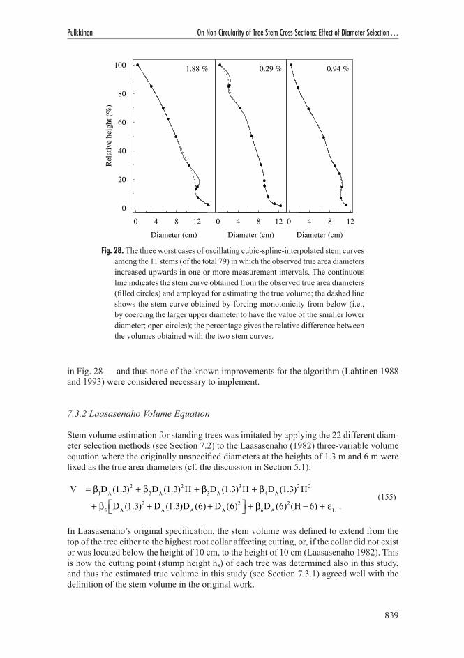
839


in Fig. 28 — and thus none of the known improvements for the algorithm (Lahtinen 1988 and 1993) were considered necessary to implement.

7.3.2 Laasasenaho Volume Equation

Stem volume estimation for standing trees was imitated by applying the 22 different diam-eter selection methods (see Section 7.2) to the Laasasenaho (1982) three-variable volume equation where the originally unspecified diameters at the heights of 1.3 m and 6 m were fixed as the true area diameters (cf. the discussion in Section 5.1):

V = β1DA (1.3)2 + β2DA (1.3)2 H + β3DA (1.3)3H + β4DA (1.3)2 H2

+ β5 DA (1.3)2 + DA (1.3)DA (6)+ DA (6)2⎡⎣ ⎤⎦ + β6DA (6)2(H − 6) + εL . (155)

In Laasasenaho’s original specification, the stem volume was defined to extend from the top of the tree either to the highest root collar affecting cutting, or, if the collar did not exist or was located below the height of 10 cm, to the height of 10 cm (Laasasenaho 1982). This is how the cutting point (stump height hs) of each tree was determined also in this study, and thus the estimated true volume in this study (see Section 7.3.1) agreed well with the definition of the stem volume in the original work.

Rela

tive

heig

ht (%

)

0 4 8 12Diameter (cm)

0

20

40

60

80

100 1.88 %


0.29 %


0.94 %

Fig. 28. The three worst cases of oscillating cubic-spline-interpolated stem curves among the 11 stems (of the total 79) in which the observed true area diameters increased upwards in one or more measurement intervals. The continuous line indicates the stem curve obtained from the observed true area diameters (filled circles) and employed for estimating the true volume; the dashed line shows the stem curve obtained by forcing monotonicity from below (i.e., by coercing the larger upper diameter to have the value of the smaller lower diameter; open circles); the percentage gives the relative difference between the volumes obtained with the two stem curves.

840


Instead of employing Laasasenaho’s parameter estimates based on the data of 2326 Scots pine sample trees from all over Finland, we re-estimated the parameters from the 50 stems of our data in which the cross-section had been observed at both the heights of 1.3 m and 6 m; this was to make the error inherent in the model (the random error term εL, also referred to as the model error) as small as possible. The estimation was performed both without and with the assumption of cross-section convexity: in the former, the estimated true volume V was employed as the response variable and the true area diameters DA(1.3) and DA(6) (as well as the height H) were used as the explanatory variables; in the latter, the response variable was the estimated true convex volume VC and the explanatory variables comprised the convex area diameters DAc(1.3) and DAc(6). As the error terms were assumed hetero-scedastic (variance proportional to DA(1.3)4H2, or to DAc(1.3)4H2; refer to Section 5.1), a weighted least squares estimation was performed with 1/[DA(1.3)4H2], or 1/[DAc(1.3)4H2], as the weight of each observation (stem); this corresponds to the ordinary least squares estimation of a form factor model carried out in the original work (Laasasenaho 1982, p. 43–44). As in the original study, the within-plot and within-cluster interdependencies of the stems, which at least in principle breached the model assumptions, were disregarded in the estimation. Judging from the residual plots, the models fitted well in the data; also, the relative root mean squared errors (the standard deviations of the relative residuals adjusted with the number of parameters) were in concordance with that in the original data (3.59% and 3.60% vs. 3.53%; Laasasenaho 1982, p. 43). The original and the re-estimated parameter values are given in Table 18. In the following, we will deal with the volume estimation without the convexity assumption; the particularities related to the estimation with the convexity assumption will be considered in the end of the section.

We assumed the re-estimated model to be correct and thus disregarded the effects of using estimated parameters instead of the true ones (cf. the discussion in Section 5.1). As the reference volume (to which the estimators by different diameter selection methods were to be compared) we used the best estimate

VL = β1DA (1.3)2 + β2DA (1.3)2 H + β3DA (1.3)3H + β4DA (1.3)2 H2

+ β5 DA (1.3)2 + DA (1.3)DA (6)+ DA (6)2⎡⎣ ⎤⎦ + β6DA (6)2(H − 6) ; (156)

this was because we wanted to distinguish the error component caused by diameter selection from the error component inherent in the model (the model error that is present even if the

Table 18. Original parameter estimates of the Laasasenaho (1982) three-variable volume equation for Scots pine (Eq. 155), and the estimates used in this study (obtained from the 50 stems in the data with both the 1.3 m and 6 m cross-sections available).

Parameter Data

2326 stems in the study V, DA(1.3), DA(6), H in 50 stems VC, DAc(1.3), DAc(6), H in 50 stems by Laasasenaho (1982) of this study of this study

β1 0.268621 0.202318 0.201441β2 –0.0145543 –0.0109918 –0.0108715β3 –0.0000478628 –0.000279395 –0.000284556β4 0.000334101 0.000831394 0.000844558β5 0.0973148 0.115504 0.115359β6 0.0440716 0.0294864 0.0291432

841


diameters were measured “correctly”, i.e., even if the true area diameters at the heights of 1.3 m and 6 m in the stem were known). The model error in each stem was then estimated as the relative error of this best estimate VL with respect to the estimated true volume V (i.e., as the relative residual (VL–V)/VL of the estimated model). The purpose of the diameter specification as true area diameters (to comply with the estimation of true volume) and the parameter re-estimation was expressly to make this error as small as possible, that is, to set the reference volume as close to our estimated true volume as possible.

Applying the different diameter selection methods to the volume equation resulted in the volume estimators (here written as a function of the diameters only)

VLj = c1Dj(1.3)2 + c2Dj(1.3)3 + c3Dj(1.3)Dj(6) + c4Dj(6)2 , (157)

where c1 = β1+ β2H+ β4H2 + β5 , c2 = β3H, c3 = β5, and c4 = β5 + β6(H −6) , and where Dj(1.3) and Dj(6) are the diameters selected with method j at the heights of 1.3 m and 6 m.

With the diameter selection methods involving only fixed diameters (methods 0, 6–11, min and max; independent and dependent selection), there was naturally no within-tree variation in the estimator values, whereby the within-tree expectation of the estimator equalled the constant estimate itself (i.e., E(VLj)=VLj and Var(VLj)=0).

With the diameter selection methods involving random diameters (methods 1–5, independ-ent and dependent selection; methods 1ξ–5ξ 1ξ90, 4ξ90 and 5ξ90, dependent selection), the within-tree expectation and variance of the volume estimator were estimated by means of estimated diameter moments and product moments:

E[VLj] = c1E[Dj(1.3)2] + c2E[Dj(1.3)3]

+ c3E[Dj(1.3)Dj(6)] + c4E[Dj(6)2] , (158)

and

Var[VLj] = c22E[Dj(1.3)6] + 2c1c2E[Dj(1.3)5] + c1

2E[Dj(1.3)4]

+ 2c2c3E[Dj(1.3)4 Dj(6)] + 2c2c4E[Dj(1.3)3Dj(6)2]

+ 2c1c3E[Dj(1.3)3Dj(6)] + (c32 + 2c1c4 )E[Dj(1.3)2 Dj(6)2]

+ 2c3c4E[Dj(1.3)Dj(6)3] + c42E[Dj(6)4]

− E[VLj]{ }2 ;

(159)

refer to Appendices E and F for the more detailed method-specific expressions. The diameter moments and product moments were estimated as explained in Section 7.2: With the meth-ods 1–5 involving the uniform direction distribution, the moment estimates were obtained as simple means from the 180 systematic diameters in each cross-section. With methods 1ξ–5ξ, 1ξ90, 4ξ90 and 5ξ90 involving the non-uniform direction distributions of the Bit-terlich diameters, the moments were estimated as weighted means from the 180 systematic diameters, the weights being determined as the relative sector areas of the inclusion region of the breast height cross-section.

The assumption of cross-section convexity influenced the reference volume, the estimated model error, and the within-tree expectations and variances of the estimators: The convex reference volume VCL was obtained from the volume equation estimated with true convex volume VC and the convex area diameters, and the relative model error [VCL–VC]/VCL

842


was naturally determined as the relative residual of this model. Since the diameters of a non-convex cross-section and its convex closure coincide, the within-tree expectation and variance of the estimator VCLj produced by each diameter selection method j were obtained by using the same diameters and diameter moment estimates as in the non-convex case, but with the parameter estimates c1, c2, c3 and c4 of the volume equation estimated with the true convex volume and the convex area diameters.

7.3.3 Cubic-Spline-Interpolated Stem Curve

Stem volume estimation for a felled sample tree was mimicked by applying each of the 22 diameter selection methods (see Section 7.2) at the 7–10 observation heights in a stem and constructing the cubic-spline-interpolated stem curves from the resulting diameter vectors (with the assumed diameter of 0.4 cm at the top of the tree added in them). Let us denote with Dj the diameter vector obtained with the diameter selection method j, with H the vector containing the observation heights (plus the tree height) and with S3[h; Dj, H] the interpolated stem curve. The volume estimate by each diameter selection method was then obtained as the solid of revolution of the stem curve from the recorded stump height hs to the height H of the tree:

VSj =π4

S3hs

H

∫ [h; D j, H]2dh . (160)

Technically the volume estimation was carried out in the same manner as the estimation of the true volume (see Section 7.3.1; however, potential oscillation in the stem curves due to diameter increase within short distances upward was not controlled here). All the 79 stems with cross-sections observed at 7 or more heights were included in the investigation.

With the diameter selection methods involving fixed diameters (methods 0, 6–11, min and max; independent and dependent selection), there was no within-tree variation in the volume estimates (i.e., Var(VSj)=0), and the within-tree expectation was given by the con-stant volume estimate itself (i.e., E(VSj)=VSj).

With the diameter selection methods involving random diameters (methods 1–5, independ-ent and dependent selection; methods 1ξ–5ξ, 1ξ90, 4ξ90 and 5ξ90, dependent selection), the diameter vector selection was repeated several times in each stem in order to capture the within-tree variation in volume estimates. The “population” from which the diameter vectors were sampled varied according to the diameter selection method: it consisted of all the diameter vectors that could be formed by the diameter selection method in question from the systematically measured diameters, 180 at each observation height, in the stem.

The dependent selection of diameters at the different heights in a stem restricted the diameter vector population so that all the vectors therein could be included in the sample: with the methods where only one diameter direction within a cross-section was actually selected and where the other direction, if taken, was fully determined by the first one (methods 1–3, 1ξ–3ξ and 1ξ90), there were 180 possible diameter vectors; with methods where two diameter directions within a cross-section were selected independently of each other (methods 4, 5, 4ξ, 5ξ, 4ξ90 and 5ξ90), the number of possible diameter vectors was 1802, as for each first diameter direction selection there were 180 alternatives as the second choice. Using these 180 or 1802 diameter vectors meant selecting the one diameter direction or the pair of diameter directions equidistantly (by every 1°) within [0°, 180°) or [0°, 180°)×[0°, 180°). To each diameter vector, the estimated selection probability of the one diameter direction or the pair of diameter directions was associated as a weight.

843


The probability was determined by means of the diameter direction distribution(s): with one direction selection, the weight was the probability of selecting a direction within 0.5° from the chosen direction (the probability mass within 0.5° from the common direction of the diameters in the diameter vector); with two independent direction selections within a cross-section, the weight was the product of such probabilities related to the two chosen directions. The within-tree expectation and variance of each volume estimator (diameter selection method) were then estimated as the weighted mean and variance of the volume estimates obtained with the diameter vectors of the method (cf. Eqs. 127 and 128 and the discussion on numerical integration in Section 5.3). (Thus, with interrelated diameter selec-tion methods (1, 1ξ and 1ξ90; 2, 2ξ and 2ξ90; 3, 3ξ and 3ξ90 etc.), the volume estimates were computed using the same diameter vectors, but the within-tree expectation and vari-ance were estimated with different weights.) With only the uniform direction distribution involved (methods 1–5), the weights associated to each diameter vector became equal, and the weighted mean and variance of the volume estimates were simplified to the simple arithmetic mean and sample variance. With the non-uniform direction distributions of the Bitterlich diameters involved in the first direction selection (methods 1ξ–5ξ, 1ξ90, 4ξ90 and 5ξ90), the weights became unequal and were obtained from the relative sector areas of the inclusion region of the breast height cross-section of the tree (cf. Section 7.2).

In the independent selection of diameters at the different heights in a stem (applied only to the diameter selection methods 1–5 involving the uniform direction distribution), the diameter vector population grew so large that all the vectors therein could not be used: with methods 1–3 the number of possible diameter vectors amounted to 180m and with methods 4–5 to1802m, m being the number of observation heights, total height excluded. Instead, we drew upon Monte Carlo integration where 1802 diameter direction vectors were to be sampled independently from the multidimensional direction distribution of each diameter selection method. With the uniform marginal distributions of the independent directions, the multidimensional direction distributions became also uniform, implying that all the diameter vectors of generated by the method had the same probability to be chosen. Therefore a simple random sample of 1802 vectors was drawn from the diameter vector population of each diameter selection method, with replacement for practical ease; in practice, the sampling was carried out by selecting randomly at each observation height the required one or two diameters among the 180 alternatives and by repeating this pro-cedure 1802 times for each stem. The within-tree expectation and variance of the volume estimator were then estimated as the mean and sample variance of the volume estimates computed from the selected diameter vectors (cf. Eqs. 129 and 130 and the discussion on Monte Carlo integration in Section 5.3).

As the natural reference volume, we employed the estimated true volume V computed with the similar stem curve approach from the true area diameters (see Section 7.3.1). Unlike with the volume equation, the error contained in the reference volume could not now be quantified, as the true volumes of the stems were unknown and no more precise estimates were available. Consequently, the within-tree biases and variances produced by the different diameter selection methods could only be compared with each other; no notion about their magnitude with respect to the “error intrinsic in the volume estimation method” could be gained.

Since the diameters are the same for a non-convex cross-section and its convex closure, assuming cross-section convexity influenced only the reference volume: with the convexity assumption, we employed the convex volume estimate VC computed from the convex area diameters (see Section 7.3.1) as the reference.

844


7.3.4 General Volume Estimator

Finally, we considered estimating the volume of the stem segment from the lowermost observation height h(1) to the uppermost one h(m) by means of general volume estimators that involved area estimation functions Âj(h)=πDj(h)2/4 arising from the application of each of the 22 diameter selection methods (see Section 7.2; j refers to the diameter selection method) and the circle area formula at a all the heights h∈[0, H] in a stem:

VGj = A jh(1)

h( m )

∫ (h)dh = π4

Djh(1)

h( m )

∫ (h)2dh . (161)

We omitted to define explicitly the values of the area estimation functions between the observation heights (and to estimate the stem volumes actually) but focused on “direct” estimation of the bias, covariance and variance functions μΔÂj(h), γÂj(h, k) and σÂj2(h) of the area estimation process {Âj(h), h∈[0, H]}={πDj(h)2/4, h∈[0, H]} of each diameter selection method in each tree. As explained in Section 5.2, the within-tree bias and variance of each general volume estimator (diameter selection method) in each tree could then be estimated by integrating the estimated treewise bias end covariance functions:

E VGj − V⎡⎣ ⎤⎦ = µΔA j

h(1)

h( m )

∫ (h)dh

= E A j(h)− A(h)⎡⎣ ⎤⎦h(1)

h( m )

∫ dh ,

(162)

and

Var(VGj) = γA j

h(1)

h( m )

∫h(1)

h( m )

∫ (h, k)dhdk

= Covh(1)

h( m )

∫h(1)

h( m )

∫ [A j(h), A j(k)]dhdk .

(163)

Further, an estimate for the theoretical upper bound of the within-tree variance (the variance conditional on fully correlated area estimation process) was given by the definite integral of the estimated variance function:

Var[VGj |ρA j

(h, k) = 1] = σA j

2 (h)h(1)

h( m )

∫ dh⎧⎨⎪

⎩⎪

⎫⎬⎪

⎭⎪

2

= Var[A j(h)]h(1)

h( m )

∫ dh⎧⎨⎪

⎩⎪

⎫⎬⎪

⎭⎪

2

.

(164)

As in the cubic-spline-interpolated stem curves before, all the 79 stems with 7 or more observed cross-sections were included in the examination. For each diameter selection method j in each stem, the bias, variance and covariance functions were estimated from the

845


discrete observations on the area estimator Âj(h)=πDj(h)2/4 along the stem, that is, from the vectors of the estimated within-cross-section biases (E[Âj(h)]–A(h))h∈H and variances (Va r [Âj(h)])h∈H at the 7–10 observation heights H=(h(1), h(2), ..., h(m)) and from the matrix of the estimated between-cross-sections covariances (Co v[Âj(h), Âj(k)])h, k∈H at the 42–90 two-height combinations H×H in the stem.

With the diameter selection methods involving only fixed diameters (methods 0, 6–11, min, max; independent and dependent selection), the variances and covariances of the area estimators at separate heights were naturally zero and the biases were given by the differ-ences between the area estimates and the true area at each height.

With the diameter selection methods involving random diameters, only dependent selec-tion was considered: With Bitterlich diameters (methods 1ξ–5ξ, 1ξ90, 4ξ90 and 5ξ90), independent selection was not feasible, as noted before. With diameters having the uniform direction distribution (methods 1–5), independent selection was to result, by definition, in the same within-cross-section biases and variances of the area estimators as dependent selection, as well as in zero covariances between the area estimators at separate heights, thus providing no information for covariance function estimation (refer to the discussion on an area estimation process with uncorrelated elements in Section 5.2). In all the cross-sections, the biases and the variances of the area estimators had already been estimated when considering cross-section area estimators (Section 7.2). Similarly, the covariances of the area estimators at different heights could be expressed in terms of diameter moments and product moments, which were then estimated from the 180 systematic diameters and their products in each cross-section (cf. Section 7.2): With the methods involving the uni-form direction distribution, the moment estimates were obtained as simple means. With the methods involving the non-uniform direction distributions of the Bitterlich diameters, the moment estimates were obtained as weighted means, the weights being determined as the relative sector areas of the inclusion region of the breast height cross-section.

From the discrete estimated values, the bias, variance and covariance functions of the area estimation process in each tree were estimated by linear interpolation. Linear interpolation was employed for simplicity and for its assuredly reasonable behaviour: as there were 56 functions to be estimated in each of the 79 stems (3 functions for each of the methods 1–5, 1ξ–5ξ, 1ξ90, 4ξ90 and 5ξ90 with dependent selection; 1 function for the method 0; and 1 function for each of the methods 6–11, min and max with both dependent and independ-ent selection), the use of smoother higher order interpolating splines requiring control and adjustment for possible non-feasible oscillations was regarded as too laborious an approach.

The linear functions could be integrated analytically. The integration limits were set as the lowermost and the uppermost observation heights h(1) and h(m), because the functions could not be justifiably extrapolated to cover the whole stem from the stump height to the very top. Thus, unlike with the other volume estimation methods, the volume bias and variance were computed only for that part of the stem within which cross-sections had been observed. As the reference volume, the estimated true volume V of the stem segment between the lowermost and the uppermost observation heights (see Section 7.3.1) was used.

The assumption of cross-section convexity did not influence the actual area estimation processes {Âj(h), h∈H} (based on diameters and the circle area formula, the area estimators Âj(h) were the same whether the cross-sections were assumed convex or not) but affected the area estimation error processes {Âj(h)–AC, h∈H}, where the errors were now taken with respect to the convex area AC. Consequently, with the convexity assumption, only the bias functions of the 30 area estimation processes (22 diameter selection methods with dependent selection, 8 methods with independent selection) needed to be re-estimated from the biases taken with respect to the convex area in each stem; the integrals of these functions

846


were then thought to yield the estimated biases E[VGj–VC] of the general volume estima-tors with respect to true (partial) convex volume VC. The reference volume, to which the estimated within-tree volume biases and variances were proportioned, was naturally also changed for the estimated partial convex volume VC (see Section 7.3.1).

7.4 Estimation of Stand Totals in Bitterlich Sampling

In Bitterlich sampling, applying circularity assumption to non-circular cross-sections was found to inflict potential bias in stand total estimators, due to two tree-specific faults in the estimated inclusion probabilities (see Eq. 69 in Section 4.1.2): (i) deviation of the true basal area factor of the tree κ(α)=AC/|M(α)| (the ratio of the convex area of the breast height cross-section to the inclusion area) from that of a circle sin2(α/2), and (ii) estimation of the convex area of the breast height cross-section with estimator Âj=πDj2/4 based on diameter Dj measured in the cross-section by some method j. With the viewing angle α values of 1.146°, 1.621°, 2.292° and 3.624° (corresponding, with circular cross-sections, to the basal area factor values of 1, 2, 4, and 10 m2/ha, respectively), these errors were investigated in the 80 breast height cross-sections of the data. As a “thinking experiment”, the examination was then extended to all the 709 cross-sections, using their own inclusion regions as if they were all breast height cross-sections.

The deviation of the true basal area factor from that of a circle, expressed as the ratio sin2(α/2)/κ(α), was first computed separately in each cross-section. In the estimation of the relative basal area of a stand by Bitterlich sampling, sin2(α/2)/κ(α)–1 straightforwardly indicates the contribution of the tree to the bias of the basal area estimator, since

E(G)−G = 1|L |

ACii∈I∑ sin2(α / 2)

κ i (α)−1

⎡

⎣⎢

⎤

⎦⎥

(165)

(cf. Eqs. 77 and 81 in Section 4.1.3). To check Matérn’s approximate theoretical result that, with viewing angle α of the magnitude 1°, this bias is the same as we would get by calipering every stem in the stand in a randomly chosen direction, that is,

E(G)−G ≈ 1|L |

Eθ (A1i )−ACi⎡⎣ ⎤⎦

i∈I∑

(166)

(cf. Eq. 85 in Section 4.1.3), sin2(α/2)/κ(α)–1 in each cross-section was compared to the relative within-cross-section bias [Eθ(Â1)–AC]/AC of the area estimator Â1 based on one random diameter, computed already earlier (see Section 7.2).

The combined effect sin2(α/2)/κ(α)·AC/(πDj2/4) was computed with the 22 diameter selection methods (see Section 7.2) in each cross-section. With the methods involving randomness (1–5, 1ξ–5ξ, 1ξ90, 4ξ90 and 5ξ90), the expectation of the effect

E sin2(α / 2)κ(α)

⋅AC

πDj2 / 4

⎡

⎣⎢⎢

⎤

⎦⎥⎥= 4πsin2(α / 2) |M(α) | E 1

Dj2

⎡

⎣⎢⎢

⎤

⎦⎥⎥

(167)

over the diameter direction distribution was considered. The fractional moments E[1/Dj2] were estimated in a similar way as moments and product moments in Section 7.2 (cf. Eqs. 148, 149 and 152). With the methods involving the uniform direction distribution (1–5),

847


the moments were estimated as the simple means of the 180 or 1802 systematic diameters raised to the power of –2 in each cross-section:

E[D(θ)−2] = 1180

Dj=0

179

∑ ( j ⋅1°)−2 ,

E D(θ)+ D(θ+ π / 2)2

⎡

⎣⎢

⎤

⎦⎥

−2⎧⎨⎪

⎩⎪

⎫⎬⎪

⎭⎪= 1

180D( j ⋅1°)+ D[( j+ 90) ⋅1°]

2⎧⎨⎩

⎫⎬⎭

−2

j=0

179

∑ ,

E D(θ)D(θ+ π / 2)⎡⎣

⎤⎦−2⎧

⎨⎩

⎫⎬⎭= 1

180D( j ⋅1°)−1D[( j+ 90) ⋅1°]−1

j=0

179

∑ ,

ED(θ1)+ D(θ2 )

2⎡

⎣⎢

⎤

⎦⎥

−2⎧⎨⎪

⎩⎪

⎫⎬⎪

⎭⎪= 1

1802

D( j ⋅1°)+ D(k ⋅1°)2

⎡

⎣⎢

⎤

⎦⎥

−2

j=0

179

∑k=0

179

∑ ,

E D(θ1)D(θ2 )⎡⎣

⎤⎦−2⎧

⎨⎩

⎫⎬⎭= 1

1802 D( j ⋅1°)−1D(k ⋅1°)−1

j=0

179

∑k=0

179

∑ = 1180

Dj=0

179

∑ ( j ⋅1°)−1⎡

⎣⎢

⎤

⎦⎥

2

.

(168)

(Note that for j+90≥180, D[(j+90)·1°]=D[(j–90)·1°].) With the methods involving the non-uniform direction distributions of the Bitterlich diameters (1ξ–3ξ, 1ξ90), the moments were estimated as the weighted means of the diameter powers, the weights being determined as the relative sector areas of the inclusion region:

E[D(ξ)−2] = wj=0

179

∑ ( j ⋅1°)D( j ⋅1°)−2 ,

E D(ξ)+ D(ξ + π / 2)2

⎡

⎣⎢

⎤

⎦⎥

−2⎧⎨⎪

⎩⎪

⎫⎬⎪

⎭⎪= w

j=0

179

∑ ( j ⋅1°) D( j ⋅1°)+ D[( j+ 90) ⋅1°]2

⎧⎨⎩

⎫⎬⎭

−2

,

E D(ξ)D(ξ + π / 2)⎡⎣

⎤⎦−2⎧

⎨⎩

⎫⎬⎭= w

j=0

179

∑ ( j ⋅1°)D( j ⋅1°)−1D[( j+ 90) ⋅1°]−1 ,

E[D(ξ + π / 2)−2] = wj=0

179

∑ ( j ⋅1°)D[( j+ 90) ⋅1°]−2 .

(169)

(Note that the weights w(j·1°), j=0, ..., 179, sum to one.) And with the methods involving both types of diameters (4ξ–5ξ, 4ξ90–5ξ90), the moments were estimated as the simple means of the weighted means (which in the case of the geometric mean of independent diameters turned into the product of the weighted and the simple mean):

848


E D(ξ)+ D(θ)2

⎡

⎣⎢

⎤

⎦⎥

−2⎧⎨⎪

⎩⎪

⎫⎬⎪

⎭⎪= 1

180w

j=0

179

∑k=0

179

∑ ( j ⋅1°) D( j ⋅1°)+ D(k ⋅1°)2

⎡

⎣⎢

⎤

⎦⎥

−2

,

E D(ξ)D(θ)⎡⎣

⎤⎦−2⎧

⎨⎩

⎫⎬⎭= w

j=0

179

∑ ( j ⋅1°)D( j ⋅1°)−1⎡

⎣⎢

⎤

⎦⎥

1180

Dk=0

179

∑ (k ⋅1°)−1⎡

⎣⎢

⎤

⎦⎥ ,

E D(ξ + π / 2)+ D(θ)2

⎡

⎣⎢

⎤

⎦⎥

−2⎧⎨⎪

⎩⎪

⎫⎬⎪

⎭⎪= 1

180w

j=0

179

∑k=0

179

∑ ( j ⋅1°) D[( j+ 90) ⋅1°]+ D(k ⋅1°)2

⎧⎨⎩

⎫⎬⎭

−2

,

E D(ξ + π / 2)D(θ)⎡⎣

⎤⎦−2⎧

⎨⎩

⎫⎬⎭= w

j=0

179

∑ ( j ⋅1°)D[( j+ 90) ⋅1°]−1⎧⎨⎪

⎩⎪

⎫⎬⎪

⎭⎪1

180D

k=0

179

∑ (k ⋅1°)−1⎡

⎣⎢

⎤

⎦⎥ .

(170)

The distributions of sin2(α/2)/κ(α) and E[sin2(α/2)/κ(α)·AC/(πDj2/4)] were viewed in the set of the breast height cross-sections and in the set of all the cross-sections. The relation between sin2(α/2)/κ(α) and cross-section shape, as expressed by the scalar shape indices (see Table 14 in Section 7.1), was studied with pairwise correlations and accompanying scatterplots.

Documents

S ILV FENNICA - Metla · In the common methods of forest mensuration, ... Circle Area Formula ... 9 Summary and Conclusions