RTX Positioning: The Next Generation of

cm-accurate Real-Time GNSS Positioning

Rodrigo Leandro, Herbert Landau, Markus Nitschke, Markus Glocker, Stephan Seeger, Xiaoming Chen,

Alois Deking, Mohamed BenTahar, Feipeng Zhang, Kendall Ferguson, Ralf Stolz, Nick Talbot,

Gang Lu, Timo Allison, Markus Brandl, Victor Gomez, Wei Cao, Adrian Kipka

Trimble Terrasat GmbH, Germany

ABSTRACT

The first commercial GPS Real-time Kinematic (RTK)

positioning products were released in 1993. Since then

RTK technology has found its way into a wide variety of

application areas and markets including Survey, Machine

Control, and Precision Farming. Current RTK systems

provide cm-accurate positioning typically with

initialization times of seconds. However, one of the main

limitations of RTK positioning is the need of having

nearby infra-structure. This infra-structure normally

includes a single base station and radio link, or in the case

of network RTK, several reference stations with internet

connections, a central processing center and

communication links to users. In single-base, or network

RTK, the distances between reference stations and the

rover receiver are typically limited to 100 km.

During the last decade several researchers have advocated

Precise Point Positioning (PPP) techniques as an

alternative to reference station-based RTK. With the PPP

technique the GNSS positioning is performed using

precise satellite orbit and clock information, rather than

corrections from one or more reference stations. The

published PPP solutions typically provide position

accuracies of better than 10 cm horizontally. The major

drawback of PPP techniques is the relatively slow

convergence time required to achieve kinematic position

accuracies of 10 cm or better. PPP convergence times are

typically on the order of several tens of minutes, but

occasionally the convergence may take a couple of hours

depending on satellite geometry and prevailing

atmospheric conditions. Long initialization time is a

limiting factor in considering PPP as a practical solution

for positioning systems that rely on productivity and

availability. Nevertheless, PPP techniques are very

appealing from a ground infrastructure and operational

coverage area perspective, since precise positioning could

be potentially performed in any place where satellite

correction data is available.

For several years, efforts have been made by numerous

organizations in attempting to improve the productivity of

PPP-like solutions. Simultaneously, efforts have been

made to improve network RTK performance with

sparsely located reference stations. Until now there has

not been a workable solution for either approach.

Commercial success of the published PPP solutions for

high-accuracy applications has been limited by the low

productivity compared to established RTK methods.

In this paper we present a technology that brings together

the advantages of both types of solutions, i.e., positioning

techniques that do not require local reference stations

while providing the productivity of RTK positioning. This

means coupling the high productivity and accuracy of

reference station-based RTK systems with the extended

coverage area of solutions based on global satellite

corrections. The outcome of this new technology is the

positioning service CENTERPOINT RTXTM

, which

provides real-time cm-level accuracy without the direct

use of a reference station infrastructure, that is suitable for

many GNSS market segments. Furthermore, the RTX

solution is applicable to multi-GNSS constellations. The

new technology involves innovations in RTK network

processing, as well as advancements in the rover RTK

positioning algorithms.

INTRODUCTION

The RTX (Real Time eXtended) positioning solution is

the technology resulting from the employment of a variety

of innovative techniques, which combined provide users

with cm-level real time position accuracy anywhere on or

near the earth’s surface.

This new positioning technique is based on the generation

and delivery of precise satellite corrections (i.e. orbit,

clocks, and others) on a global scale, either through a

satellite link or the internet. The innovative aspects of the

new solution can be divided into different categories,

which directly relate to the areas that have represented

different levels of limitation on making global high

accuracy positioning possible. These areas are:

a) Integer level ambiguities derivation;

b) Real-time, high accuracy satellite corrections

generation;

c) Data transmission optimization;

d) Positioning technology.

During the following sections we will explore each of

those areas, highlighting the new aspects of the solution,

as well as pointing out differences with respect to existing

technologies, some of which are available in commercial

services. In that sense we will explain why, and how,

RTX is a solution different from both differential RTK

and precise point positioning as currently understood by

the general GNSS community.

SYSTEM OVERVIEW

The RTX technology is employed to offer cm-level GNSS

positioning through the CENTERPOINT RTXTM

service.

The general infra-structure of the system can be in the

schematic flowchart below.

Figure 1. CENTERPOINT RTX

TM infra-structure.

Data from monitoring stations distributed around the

globe are collected and transmitted via the internet to

operation centers at different locations. The complete

operation centers (encapsulated by the dashed red square

in Figure 1) are redundant in order to assure the very high

(~100%) availability of the system. In case it is needed,

the correction stream source might change between

operation centers and/or processing servers within

centers. These operational changes are completely

handled in a deterministic way by all parts of the system

including the user receiver. Inside the operation centers

redundant communication servers are used to relay the

network observation data to the data processing servers,

which host the network processors that produce precise

orbit, clock, and observation biases valid for any place on

the globe.

After being generated, the precise satellite data are

compressed in messages compliant with the CMRx

format, especially developed for compact transmission of

satellite information. The messages are finally routed to

either an uplink station or made available for internet

connection access by the users.

The CENTERPOINT RTXTM

tracking network is

currently composed of around 100 stations, fairly well

distributed across the globe. Figure 2 shows the location

of stations used in the system.

Figure 2. CENTERPOINT RTX

TM tracking network distribution.

The CENTERPOINT RTXTM

service is currently offered

in the central region of North America, via satellite link,

as indicated in Figure 3.

Since October 2011 the CENTERPOINT RTXTM

service

has been also offered to users in Australia. In this region

the service is currently offered for users with access to

internet connection (Figure 4).

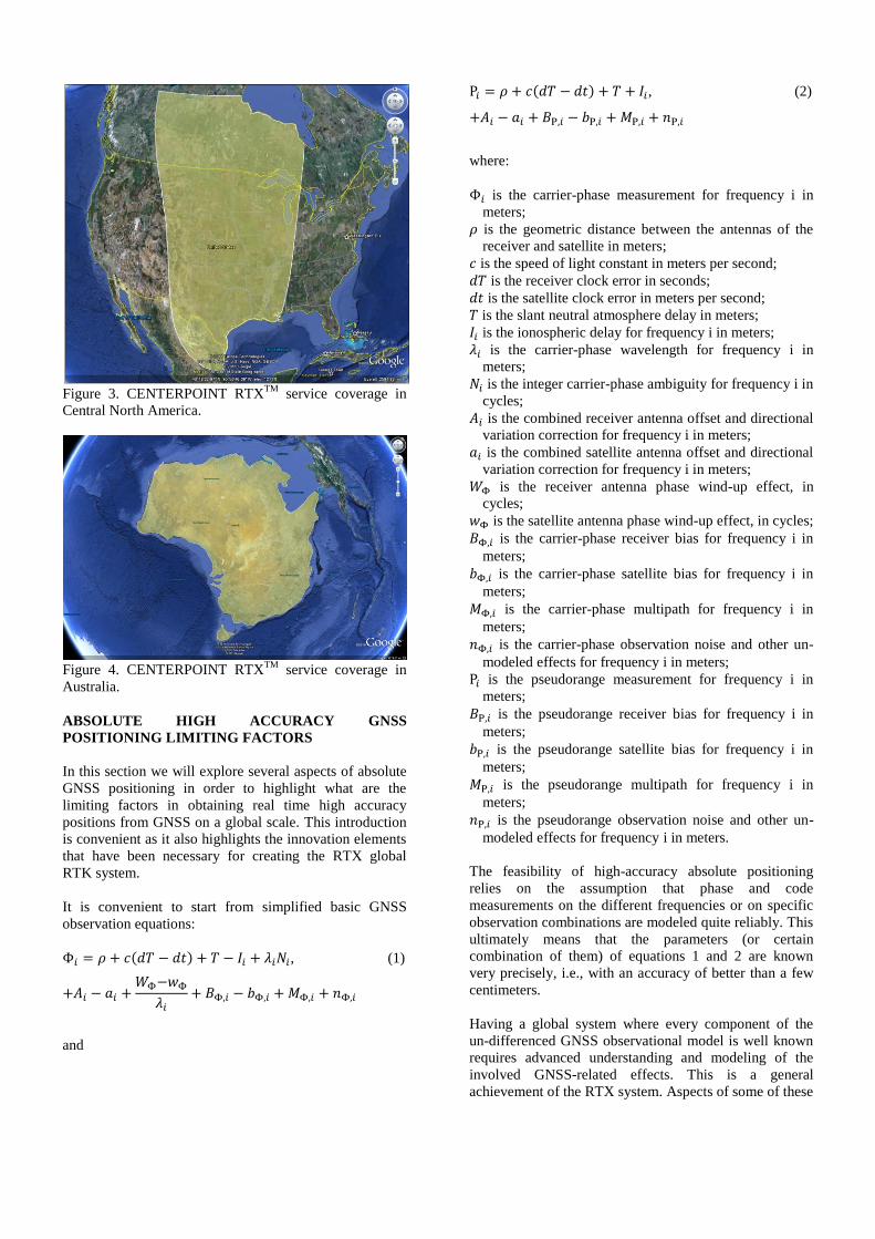
Figure 3. CENTERPOINT RTX

TM service coverage in

Central North America.

Figure 4. CENTERPOINT RTX

TM service coverage in

Australia.

ABSOLUTE HIGH ACCURACY GNSS

POSITIONING LIMITING FACTORS

In this section we will explore several aspects of absolute

GNSS positioning in order to highlight what are the

limiting factors in obtaining real time high accuracy

positions from GNSS on a global scale. This introduction

is convenient as it also highlights the innovation elements

that have been necessary for creating the RTX global

RTK system.

It is convenient to start from simplified basic GNSS

observation equations:

( ) , (1)

and

( ) , (2)

where:

is the carrier-phase measurement for frequency i in

meters;

is the geometric distance between the antennas of the

receiver and satellite in meters;

is the speed of light constant in meters per second;

is the receiver clock error in seconds;

is the satellite clock error in meters per second;

is the slant neutral atmosphere delay in meters;

is the ionospheric delay for frequency i in meters;

is the carrier-phase wavelength for frequency i in

meters;

is the integer carrier-phase ambiguity for frequency i in

cycles;

is the combined receiver antenna offset and directional

variation correction for frequency i in meters;

is the combined satellite antenna offset and directional

variation correction for frequency i in meters;

is the receiver antenna phase wind-up effect, in

cycles;

is the satellite antenna phase wind-up effect, in cycles;

is the carrier-phase receiver bias for frequency i in

meters;

is the carrier-phase satellite bias for frequency i in

meters;

is the carrier-phase multipath for frequency i in

meters;

is the carrier-phase observation noise and other un-

modeled effects for frequency i in meters;

is the pseudorange measurement for frequency i in

meters;

is the pseudorange receiver bias for frequency i in

meters;

is the pseudorange satellite bias for frequency i in

meters;

is the pseudorange multipath for frequency i in

meters;

is the pseudorange observation noise and other un-

modeled effects for frequency i in meters.

The feasibility of high-accuracy absolute positioning

relies on the assumption that phase and code

measurements on the different frequencies or on specific

observation combinations are modeled quite reliably. This

ultimately means that the parameters (or certain

combination of them) of equations 1 and 2 are known

very precisely, i.e., with an accuracy of better than a few

centimeters.

Having a global system where every component of the

un-differenced GNSS observational model is well known

requires advanced understanding and modeling of the

involved GNSS-related effects. This is a general

achievement of the RTX system. Aspects of some of these

components including their importance for global

positioning are now discussed.

Apart from the effects that are detailed below, there are a

number of corrections that have also to be considered in

order to achieve cm-level positions in a given earth-

centered reference frame. Some of these effects are solid

earth tides, ocean tidal loading, and polar motion. Details

on how these effects can be modeled can be found in Petit

and Luzum (2010).

Satellite orbits and clocks

The receiver coordinates, which are the parameters of

most interest for us, primarily depend on the geometric

distance, and thus hold a relationship with all other

parameters belonging to the same observation equation.

Some of those and their relevance for positioning are now

explored.

The geometric range in equations 1 and 2 can be

represented as a traditional norm computation formula,

thus:

√( ) ( ) ( ) (3)

where:

are coordinates of the receiver antenna reference

point in the ECEF coordinate system at the time of

signal reception, in meters;

are coordinates of the satellite center of mass in

the ECEF coordinate system at the time of the signal

transmission, in meters.

It is important to note that in a system such as RTX,

where satellite clocks are computed using a given set of

satellite orbits (in our case the RTX real-time orbits),

certain components of the orbit errors are absorbed by the

estimated clocks and have their impact on positioning

minimized. The component of the orbital error that gets

mostly minimized is somewhat near the direction of the

radial component (generally pointing towards the earth).

The exact direction of the minimum orbit error impact on

positioning is not straight forward to be determined, as it

depends on the network coverage and other aspects of the

clock processing model such as observation weighting.

However it is fair to say that the impact of the orbit error

on positioning is dependent on the angle between the

receiver-satellite line of sight (vector r in Figure 5) and

the direction of minimum orbit error impact (vector e in

Figure 5).

Figure 5. Satellite orbital error impact geometry

In order to assure high reliability in global positioning and

global network data processing it is of fundamental

importance that satellite orbital errors are minimal, since

most of the other components of the system depend on the

quality of this information.

Both satellite orbits and satellite clock errors ( in

equations 1 and 2) are considered as known by the

positioning engine. This means that any error in the

satellite clock provided by the network processing will

translate directly into an observation modeling error of

same magnitude.

Receiver clock error

The receiver clock error, in equations 1 and 2, is

usually implemented as a parameter in positioning

engines that employ an un-differenced observation model.

In that case the parameter is normally modeled as a white

noise process. In the case of (between satellites)

differential observations, the receiver clock term is

eliminated and does not need to be explicitly modeled.

In case of satellite systems operating with CDMA (Code

Division Multiple Access), such as GPS, all satellites

transmit their signals in the same frequency. Because of

this the receiver-dependent carrier-phase and code biases

are usually the same for all satellites. Thus it is possible to

eliminate these terms with a between-satellite single-

difference operation, or to assume that they are estimated

as part of the receiver clock error. In the latter case

equations 1 and 2 would read:

( )

, (4)

and

( )

, (5)

where

, (6)

and

. (7)

It is interesting to note that when making the assumption

that the receiver biases can be modeled along with

receiver clock parameters, the perceived clock error

becomes inconsistent between phase and code

measurements. In some cases this feature might play a

role, and special procedures such as keeping a bias

parameter for one of the two might have to be put in

place. There have been efforts in using observation

models using a decoupled phase-code clock approach

applied to PPP techniques, such as in Collins et al. (2008).

In case of satellite systems employing FDMA (Frequency

Division Multiple Access) signals, such as GLONASS,

different satellites use difference transmission

frequencies. This is a limiting factor for positioning in

general, but even more for global high-accuracy

positioning. The fact that the assumption of bias

absorption by the perceived receiver clock is no longer

entirely valid introduces a burden on how the

measurement biases for different satellites can be

accounted for. The problem is even more critical when

combining data collected with receivers from different

manufacturers as the experienced biases might be

significantly different for different receiver types.

Antenna phase center modeling

GNSS measurements refer to the antenna phase centers of

receivers and satellites. Such antenna phase centers

typically do not coincide with reference position points

for neither satellite nor receiver. In case of the receiver it

is usual to have the bottom of antenna mount as the

reference point. For the satellite, positions typically refer

to its center of mass. The offsets between these reference

points and the antenna phase centers have to be accounted

for, as these values can reach a couple of meters for the

spacecraft, and can be at the decimeter level for receivers.

In case of the satellites there is one additional

complicating factor which is the required knowledge of

the satellite attitude, since the antenna offsets are known

for the satellite body coordinate system, and thus a

transformation to the earth-centered coordinate system is

required before accounting for this quantity in the

measurement domain. The most challenging component

of the satellite attitude is the yaw, as for some satellites

the yaw maneuvering during and around eclipsing seasons

is not completely deterministic.

In addition to the antenna offsets, variations on the phase

center position for different observed azimuth and

elevation (or nadir angle, in case of the satellite) have also

to be taken into account. The antenna phase center

variation effects are typically in the range of few mm.

More details on standardized antenna correction can be

found for example on Rothacher and Schmid (2010). Both

type of antenna corrections, offset and variation, shall be

properly accounted for receiver and satellites in a global

cm-level GNSS application.

Phase wind-up effects

The receiver antenna phase wind-up is of peculiar

nature, since for some practical GNSS positioning

applications there might be absolutely no model that can

describe the expected wind-up effect due to the

unpredictable nature of the antenna movements. It is

important to note, however, that the phase wind-up

component caused by rotation of the antenna along its

axis (yaw) is common for all satellites in view. Rotation

in the other directions (i.e., roll, pitch) results in phase

wind-up effects that are different for each satellite,

dependent on the geometry.

The satellite phase wind-up can be computed from

models that describe the satellite attitude. There have

been some efforts from the GNSS community in the

direction of properly modeling the GNSS satellites

attitude, especially concerning the yaw attitude of some

satellite types such as GPS block IIA and GLONASS

satellites (see e.g. Bar-Sever (1995), Kouba (2008),

Dilssner et al. (2010)). If used, such models have to be

carefully employed in order to avoid problems for high-

accuracy observation modeling.

Neutral atmosphere delay

The neutral atmosphere (or troposphere, for simplicity)

incorporates the delay suffered by the GNSS signal due to

the presence of gases in the atmosphere, including water

vapor. In the case of the troposphere, the relationship

between the slant delay at a given elevation angle and the

delay that would be experienced at the zenith direction is

in general well known. This relationship is represented by

tropospheric mapping functions, thus:

, (8)

where is the mapping function for the tropospheric

delay, and is the zenith delay. Furthermore, both the

delay and the mapping function can be separated into two

components, normally referred to as wet and hydrostatic

(or dry). Equation 4 can then be re-written as:

(9)

In the case of real-time absolute positioning it is usual that

the tropospheric delay is not well known. This is because

atmospheric prediction models suitable for real-time

receiver operation (such as UNB3, UNB3m, and GPT

models – Collins and Langley (2007), Leandro et al.

(2006), and Böhm et al. (2007), respectively) provide

typical accuracies of up to a few decimeters at zenith

direction (Collins et al. (1996), Leandro (2009)), with

errors being mostly caused by the variability on the

amount of water in the atmosphere for the region and time

of interest. The lack of reliable a priori information and a

well understood relationship between slant and zenith

delays makes the modeling of the tropospheric delay as a

parameter the most suitable option for handling this effect

in absolution high accuracy positioning. In this case the

parameter estimated is typically the zenith delay or a

variation of it, such as delay scaling factor.

The limitation in such an approach is the assumption that

the mapping function is enough for describing the

behavior of the delays. This assumption becomes invalid

in cases where the slant delays do not have a symmetric

behavior with respect to the receiver-satellite azimuthal

direction. This typically occurs in the presence of weather

fronts where the amount of water vapor in the atmosphere

is changing more dramatically in certain directions than in

others. The asymmetric behavior of the troposphere

imposes a challenge for high accuracy, real-time global

GNSS positioning.

Ionospheric delay

The ionospheric delay ( in equations 1 and 2) is one of

the important limiting factors in global positioning. This

is because information on the behavior of the ionosphere

on a global scale is quite limited in terms of accuracy,

even in post-processing products. The most reliable

products available for the GNSS community are the IGS

(International GNSS Service) ionospheric maps made

available with latencies as short as one day after data

collection. These maps have a usual accuracy of 2-8

TECUs (International GNSS Service (2011)). One TECU

(Total Electron Content Unit) is equivalent to around 0.16

m delay for the L1 frequency, remembering that being a

dispersive medium, the ionosphere causes different delays

on different frequencies. As widely known, the

ionospheric delay is inversely proportional to the squared

signal frequency. The actual relationship reads:

, (10)

where is the GNSS frequency i in MHz. It is therefore

also easy to derive the relationship of the ionospheric

delay between different frequencies:

, (11)

where subscripts i and j stand for frequencies i and j,

respectively. Another relationship caused by the

dispersive nature of the ionosphere is the inverse impact it

causes in carrier-phase and code measurements. While

code measurements suffer a signal delay, carrier-phase

measurements suffer an advance. Please note that in this

text we are referring to the ionospheric terms as delays,

and thus these terms are reduced in the carrier-phase

measurement equations, while added in the pseudorange

ones.

Even in the absence of accurate a-priori information the

handling of the ionosphere in positioning can take several

forms, depending on the positioning engine setup and the

targeted usage of the derived ionospheric information. For

instance it is possible to handle the ionospheric delay as a

parameter of the un-differenced GNSS observation

model. In this case the iono delay is derived using the

relationships established by equations 1, 2, 10, and 11,

and thus one unique ionospheric delay parameter can be

estimated with code and carrier-phase measurements from

different frequencies.

Another way of handling the ionosphere is creating

observation combinations from which the delay can be

explicitly derived. These combinations are usually formed

in a way to eliminate non-dispersive effects. This is the

case for the ionospheric phase combination, where:

(12)

and therefore:

(

)

( )

, (13)

where is the ionospheric carrier-phase combination

in meters. Multipath and noise terms have been neglected,

and antenna corrections are assumed to be properly

applied prior or after the observation combination. It is

important to note that if the combination above is to be

used for integer ambiguity derivation, the other

outstanding parameters have to be precisely known, or

also derived. This means a proper modeling and/or

estimation of the receiver and satellite phase wind-up

effects, and the ionospheric phase bias term, which can be

represented as:

, (14)

and thus:

(

)

( )

. (15)

Likewise the carrier-phase, the pseudorange

measurements can also be used to form an ionospheric

combination, as shown below.

(

) , (16)

where:

. (17)

Another very common way of handling the ionospheric

delay present in the measurements is by combining them

in a way that the delay gets eliminated. In fact only the

first order of the ionospheric delay (as represented in

equation 10) is differenced out, and second and higher

order components of the ionosphere might still be present

in the inospheric-free combination afterwards. The second

order component typically represents delays at mm to cm

level for L1 frequency (Morton et al. (2009)), and in most

real time applications are neglected.

The first variation of ionospheric-free combination we

will discuss is the combination between two frequencies

of carrier, yielding into an iono-free phase measurement,

or code, which yields into the iono-free code

measurements. The ionospheric-free carrier phase

measurement can be formed as follows:

, (18)

and thus:

( )

, (19)

where the antenna effects are assumed to be properly

corrected; is the ionospheric-free carrier phase

combination formed with measurements from frequencies

i and j - the same applies to all other terms with same

subscript. This combination has not only been widely

used in traditional GNSS, but it has also been established

as a standard for applications where traditional precise

absolute positioning is performed. The reason that makes

this combination so important is the fact that it provides

an observation that directly relates to the geometric

components of the positioning model (e.g. the receiver

coordinates) with no influence of the ionospheric delay,

using an observation which has a reasonably low noise,

especially if compared to code noise.

If one intends to derive integer level ambiguities in

absolute positioning using the iono-free carrier-phase

combination it is necessary that the phase wind-up for

receiver and satellite antennas are properly modeled or

corrected. Furthermore, assuming an approach where the

receiver phase bias will be modeled along with the

receiver clock (e.g. equations 4 and 6) or eliminated by

differencing observations between satellites, it becomes

evident that the satellite phase bias term has to be

accounted for. As it would be difficult to model this bias

as an additional parameter in a single-receiver positioning

processor, these values, or a combination of values from

each these can be derived, have to be ideally provided by

the network processors. This is the case for the RTX

system.

The ionospheric-free pseudoranges can be derived in a

similar manner as the carrier-phase:

, (20)

and thus:

( )

, (21)

Pseudoranges are commonly used in positioning solutions

for a number of different reasons. Besides the fact that

pseudorange observables are often used for computation

of the signal transmission time, their un-ambiguous nature

makes these measurements a powerful component in

GNSS positioning, for both rover positioning and network

processing. It is important to note that if iono-free code

measurements are used, observation biases with respect to

phase of same combination might have to be accounted

for. In addition to the satellite observation bias

which follows the same logic as for the respective term of

the carrier-phase measurement, it might also be necessary

to account for receiver biases between code an phase,

which in this in this case can be written as:

. (22)

The other possible approach to account for the code-phase

bias inconsistency is to directly model the perceived

clocks for code and phase measurements ( and

)

separately.

Ionospheric-free combinations can also be formed

combining code and phase measurements. This can be

done in different ways, and each combination can be

employed for different purposes in positioning and

network processing algorithms. One peculiar code-carrier

combination is between the narrow-lane code, and wide-

lane phase. Differencing these two combinations yields an

ionospheric-free and geometry-free measurement. The

wide-lane phase can be obtained as:

, (23)

and thus:

( )

. (24)

Please note that phase wind-up effects are cancelled out in

the wide-lane phase combination, and that the ionospheric

delay has its sign inverted. The narrow-lane code

observation can be created as:

, (25)

and thus:

( )

. (26)

Since the ionospheric delay assumes the same form for

both wide-lane phase and narrow-lane code, differencing

these two combinations results in an ionospheric-free

measurement. Furthermore, the geometric effects

(geometric distance, clocks, troposphere) are also

cancelled out. Therefore, this combination provides a

direct measure of the wide-lane combination of carrier-

phase ambiguities, along with the respective code and

phase measurement biases, multipath and noise:

(27)

The narrow-lane code and wide-lane phase combination

has been introduced by Garbor and Nerem (2002) as a

means of resolving ambiguities for global positioning.

After that a number of authors have adopted and refined

this approach. The power of this combination is the

detachment of the ambiguity parameter from the

geometric terms, as previously pointed out. As a

drawback, the code noise and code and phase bias

parameters have to be properly handled. There are other

code and carrier combinations that provide similar

benefits. This is the case for combinations between code

measurements of a particular frequency and carrier-phase

measurements from two frequencies. The phase data can

be combined in a specific way to cancel out geometric

and ionospheric effects of pseudoranges observed on a

given frequency, say, frequency i, as derived below. In

this text we are calling this combination as divergence-

free phase combination and it can be formulated as

follows:

, (28)

and thus:

( )

. (29)

The divergence-free phase can then be combined with the

code measurement:

(30)

While this combination provides the possibility of

working with code measurements obtained on one single

frequency, the wavelengths obtained for the divergence-

free carrier-phase ambiguities are very short. As a

reminder, for all cases of code and carrier combinations

above the resulting biases for both, or combined, carrier

and code measurements have to be properly accounted for

in ambiguity resolution-enabled GNSS processing.

REAL-TIME NETWORK PROCESSING

As mentioned earlier, the RTX system works based on

precise satellite information which is generated at

processing centers, and broadcast to users. The precise

information employed by the systems comprises satellite

orbits, satellite clocks, satellite biases, and other auxiliary

information. In this section we will explore aspects of

each of those components.

The requirements for the satellite orbits to be used in the

global RTX system can be summarized as accuracy,

continuity, robustness and reliability. The satellite

positions have to be accurate for obvious reasons,

including the fact that orbit errors have direct impact on

rover position determination quality. Furthermore,

because the RTX network process algorithms use

ambiguity resolution, the reliability of the ambiguity

determination is highly affected by the satellite orbits

quality due to the distances between reference stations in

the tracking network. The continuity requirement is put in

place to avoid the need of handling observation modeling

inconsistency over time for both network and rover

processing. For the same reason the overall system

employs techniques to properly handle switches between

redundant orbit processing servers without degradation of

position quality. As one would expect, network

processors have to be in general robust against the

eventuality of poor data entering the system for various

reasons. The RTX network processors employ a variety of

quality control techniques to ensure that only data with

the highest expected quality is used for the computation

of end products. Last but not least, the reliability is a very

important factor for real-time orbit processing. At the

current stage the RTX real-time orbit processors are able

to run for several months with virtually zero intervention

from operators, while handling events such as satellites

going through unhealthy periods and satellite maneuvers

(during unhealthy period or not).

There are at least two strong reasons for justifying the

need of implementing and running an RTX proprietary

orbit processing server. The first one is simply the need of

reliably meeting the above mentioned requirements. The

second one is that from an operational perspective, the

RTX system is conceived in such a way that it does not

rely on any external source of information to be able to

run at its full accuracy capability. In Figure 6 it is possible

to see the achieved orbit errors provided by IGS ultra-

rapid products during two weeks of March 2011, where

IGS rapid orbit products are used as truth. The ultra-rapid

orbits are evaluated using the initial portion of the

predicted arc, thus making use of the most reliable part of

the predicted arcs as the products become available in

real-time. In that case neither accuracy nor continuity

requirements for RTX processing are completely met.

Figure 6. IGS ultra-rapid orbit errors, as compared to IGS rapid orbit products.

The orbit estimation in the CENTERPOINT RTXTM

system is based on a combination of a UD-factorized

Kalman filter estimating satellite position, satellite

velocity, troposphere states, integer ambiguities, solar

radiation pressure parameters, harmonic coefficients, and

earth orientation parameters. The prediction step in the

filter is using a numerical integration of the equations of

motion in connection with a dynamic force modeling. The

basic principles of the approach are described by Landau

(1988). Forces considered in the approach are

- The earth’s gravity field

- Lunar and solar direct tides

- Solar radiation pressure

- Solid earth tides

- Ocean Tides

- General Relativity

In RTX orbit processing carrier phase integer ambiguities

are resolved in real-time. Also, the satellite orbit states are

truly estimated in real-time and continuously adapted over

time to better represent the current reality. This means

that the satellite positions that are evaluated by the user

have prediction times of no more than a few minutes since

the last orbit processing filtering update, providing

negligible loss of accuracy. In Figure 7 the orbit errors

obtained from the RTX orbit processor can be seen.

Similarly to the previous figure, IGS rapid orbit products

are used as reference. The time span is also the same as in

the previous figure. The RTX real-time orbit components

have a typical overall accuracy of around 2.5 cm, and a

3D error accuracy of around 4 cm, considering IGS rapid

products as truth.

Figure 7. RTX real-time orbit errors, as compared to IGS rapid orbit products.

Satellite clock estimation is an essential part of the RTX

system. It plays a fundamental role on positioning

performance due to a number of reasons. Satellite clocks

map directly into line-of-sight observation modeling,

yielding into a one to one error impact from clocks into

GNSS observables modeling. Due to the same strong

relationship, it is of fundamental importance that clocks

are generated in a way to facilitate ambiguity resolution

within the positioning engine. The processing speed of a

clock processor is also of fundamental importance, due to

the fact that any delay in computing satellite clocks is

directly translated into correction latencies when

computing real-time positions on the rover side. For that

matter one should keep in mind that regardless how late

satellite corrections get to the GNSS receiver in the field,

positions have to be provided to the user as soon as the

rover GNSS measurements are available. Therefore

latencies typically introduce errors into the final real time

position. In this paper we define real-time positioning as

the computation of positions at the time when the rover

observables are available, regardless the latency of the

correction stream. This is a necessary concept in order to

support dynamic rover GNSS positioning.

The RTX clock network processor was designed around

the requirements discussed above. It computes clocks that

are compatible with ambiguity resolution on the user

receiver. As a matter of fact, the clock network processor

itself employs ambiguity resolution for the generation of

the RTX clocks. The processor architecture is based on an

innovative design which allows processing data of several

hundreds of reference stations, including all necessary

steps such as data quality control, ambiguity resolution,

and the final clock generation, within a fraction of second.

The processing time of this kind of real time network

processor has to be minimized as much as possible in

order to allow the processor to operate at 1 Hz, and to

minimize the final correction latency at the rover end. It is

important to note that the final latency of the correction

stream is a composition of three basic components: the

time for the network data to arrive at the network

processing server; the network processing time; and the

correction transmission time to reach the final user.

Figure 8 shows the typical total correction latency for the

RTX system, when corrections are broadcast through a

satellite link.

Figure 8. Typical RTX correction stream latency. The

dashed green line represents the latency at 50% (3.7 s),

and the dashed red line represents the latency at 99% (5.6

s.)

Unlike satellite orbits, satellite clock solutions are more

difficult to be directly compared. This is because different

clock solutions might have offsets between each other, as

well as behave differently due to differences in their

GNSS reference time realization process as well as in

their observation modeling approaches. That said, one

way of verifying the quality of satellite clocks is to

quantify how well it can be used to model actual receiver

observation data. This can be in general achieved by

applying satellite orbit and clock correction onto GNSS

data and verifying the remaining residuals. Other

quantities such as receiver coordinates have to hold their

correct values for the residuals to be meaningful. One

remark to be made concerning this type of assessment is

that in this case not only the satellite clock quality is

assessed, but the combined satellite orbit and clock error.

For our purposes this is perfectly fine, since this is the

way orbits and clocks are employed in rover positioning

as well. Figures 9 and 10 show typical combined satellite

orbit and clock errors at line of sight for different

satellites. Figure 9 shows the ionospheric-free phase

modeling error for GPS satellites, while Figure 10 is for

GLONASS. Please note that observations of a reference

satellite (highest elevation at the time of observation)

were reduced from the others. This was done in order to

remove the receiver clock errors from the residuals. As it

can be seen, for both GPS and GLONASS cases the

observation modeling error after using RTX orbit and

clock corrections is on average at 1 cm level, with values

typically less than 2 cm. The GPS satellite with outlying

behavior in the plot below was setting at that time, and the

increased amplitude of the residuals is mostly due to

receiver observation errors such as multipath.

Figure 9. RTX clock quality (GPS) by means of corrected

ionospheric-free phase measurements.

Figure 10. RTX clock quality (GLONASS) by means of

corrected ionospheric-free phase measurements.

In addition to satellite orbits and clocks, satellite system

biases are also of interest for high accuracy global GNSS

positioning. As previously discussed, properly modeling

observation biases is one of the requirements for

achieving complete, accurate, cm-level global observation

modeling in GNSS. This is the case because observation

biases have to be either modeled or eliminated in order to

allow other parameters, such as position and ambiguities,

to be accurately determined. Examples of observation

biases are shown in most equations of this text. One

remark to be made is that even though we are refereeing

to these quantities as biases in this text, one should not

assume that these offsets are necessarily constant, or

stable, over time. In Figure 11 biases between two

combinations of observations on L1 and L2 frequencies

are shown for different satellites for June 2009. Values

are quite stable over time for PRN 02, PRN 11 and PRN

19. The line for PRN 32 shows a case where biases slowly

drift over time, which is not too uncommon. Further down

in the plot the behavior for PRN 25 is shown. In this case

not only the bias was slowly drifting until around the 17th

day of June, but it also quickly changed level around that

time. The satellite was healthy during this change. A few

days later around June 26th

the satellite was set unhealthy,

thus no continuation on the estimated bias line. These

examples show the importance of real time estimation and

monitoring of satellite system biases, since the use of pre-

established values would eventually fail in the occurrence

of events such as a level change, or gradually degrade the

performance in case of slow drifts. As mentioned earlier,

satellite observation bias real-time estimation and

monitoring is one of the components of the RTX system.

The RTX network processing servers run bias network

processors for this purpose.

Figure 11. Satellite observation bias examples from June

2009.

COMMUNICATION AND POSITIONING

Once all satellite information is available, it has to be

compressed in a message that can be broadcast to the user

in the field. The transmission of global corrections can be

done via internet, in case the user has access to it, or using

a satellite link. In the later it is usual that corrections

sufficient to cover the transmission satellite footprint are

broadcast rather than corrections complete enough to

cover the globe. Firstly, because it is expected that users

operating inside the footprint of the satellite will be using

the correction only for that region, and not anywhere else;

secondly because bandwidth restrictions usually play a

role in message design for satellite-based communication.

The bandwidth restrictions do not only enforce that the

maximum bandwidth utilization is below a certain limit,

but also require that the utilization over time is

homogeneous to ensure optimal usage of the satellite

channel. Furthermore, satellite signals are typically

susceptible to frequent message packet losses depending

on the user environment, such as when a receiver is

running under canopy. For mitigating the packet losses

the message has to be built in a way to allow the rover to

continue to operate with minimum loss of availability. In

that case not only the message design has to foresee this

type of situation, but also the message decoding, usage

and positioning algorithms have to be optimized to most

favorably couple with the received messages. All these

factors have been taken into account during the RTX

system communication design. A new message format

was created to carry information on satellite orbits,

clocks, observation biases, and other auxiliary

information. This new format was based on pre-existing

concepts developed by Trimble as part of its RTK CMRx

format. Among other aspects, the new RTX CMRx

satellite messages:

- are independent from broadcast IODEs. The user

is not required to couple the satellite messages

with broadcast information restricted to a given

IODE;

- have negligible inter-dependency. The messages

are generally decodable irrespective of which

messages have been received immediately prior

to them. This characteristic differs from message

designs using “delta” approaches, where

information from (quasi-) consecutive messages

has to be combined;

- deliver 1 mm resolution for satellite orbits and

clocks, with clocks currently configured to be

delivered at 2 seconds rate for satellite links, and

1 Hertz for internet links;

- have a bandwidth utilization (with 2 second

clocks) of around 600 bps for covering the

Americas, and 1200 bps for global coverage.

The RTX positioning engine inherits several

technological aspects from Trimble’s pre-existent RTK

engine. This aspect makes the RTX positioning mode, and

traditional RTK positioning modes (e.g. single base,

VRS) easy to co-exist. Among other things, the new

engine has been thoroughly tested and optimized for

challenging tracking environments. In these scenarios the

engine is presented with observation data collected with a

high level of multipath and low signal to noise ratio, often

resulting in cycle slips and gaps in the data. As previously

mentioned, at the same time the correction stream also

suffers packet losses and the correction data might not be

completely available during certain masking conditions.

As for positioning performance, the RTX engine delivers

typical final accuracies at 1-2 cm level for horizontal

positioning, and 2-4 cm for vertical. The final

convergence of the system is achieved in 10 to 45 minutes

after receiver startup. The time to converge might depend

on several aspects, including satellite geometry and

multipath conditions.

In order to overcome the increased convergence time as

compared to traditional RTK systems, a number of

features have been implemented as part of the RTX

positioning engine, two of which are worthy of mention

here. The Fast Restart feature allows users who have not

moved their equipment since the last RTX solution to

power up the receiver – after any amount of time – and

immediately obtain a converged solution. This feature is

quite valuable, for example in Agriculture applications,

where the user typically does not move his tractor

between RTX-steered field work activities, avoiding for

the majority of the time the need of waiting for new

convergence period before start working one or more days

after the last system usage. The second feature to be

mentioned is also related to avoiding system re-

convergence. A novel outage recovery capability makes

the RTX positioning engine able to immediately recover

from a complete constellation outage with loss of lock

during any dynamic activity. This Bridging feature

prevents the system from entering into a new convergence

phase in case the receiver loses track of up to al satellites

in view, coupled with outages of up to a couple of

minutes, such as when running behind a tree line, or under

a bridge.

POSITIONING PERFORMANCE

As mentioned earlier, the RTX system provides horizontal

accuracies of around 1-2 cm, 1-sigma. Figure 12 shows an

example of horizontal position error obtained in real time

in a receiver acquiring the RTX correction data through

the satellite link in North America. The receiver was

running continuously for several days, and was located in

Ames, Iowa, United States. As it can be seen in that

example the horizontal RMS was 1.4 cm, with a 95%

horizontal error of 2.4 cm. These are typical values for the

satellite-based RTX horizontal performance.

Figure 13 shows the vertical performance for the same

receiver and time period. As it can be seen the vertical

RMS was 2.8 cm, with 95% vertical error of 4.4 cm.

Figure 12. RTX real-time horizontal positioning performance.

Results obtained from a receiver operating in Ames, Iowa, US.

Figure 13. RTX real-time vertical positioning performance.

Results obtained from a receiver operating in AMES, Iowa, US.

Another aspect of fundamental importance for the RTX

system is the time to achieve convergence. This is

important because convergence is directly connected to

the level of productivity that can be achieved for actual

field applications. In the example to follow a continuously

powered RTX receiver was used in order to show an

assessment of the RTX (re-) convergence capability. The

receiver had tracking of all satellites disabled every hour

with an antenna switch. The duration of the outages were

three minutes during which times no GNSS satellites were

tracked. When the satellites are tracked again after the

outages, all of them come back with cycle slips, as it can

be seen in the outage phase tracking plot example in

Figure 14. The colored lines indicate the tracked L1 phase

of each satellite available at that time, and the black

marks indicate cycle slips flagged in the phase data.

Figure 14. Phase tracking example for the induced data

outages used in the re-convergence test.

This procedure is repeated hourly for several days in

order to gather enough performance runs to derive

meaningful statistics. Figure 15 shows the resulting

performance of this type of assessment using the RTX

system. Note carefully that the standard cold-start re-

convergence performance is indicated with the blue lines,

where the solid lines represent the 90% performance and

the dashed line represents the 68% performance.

As it can be seen in Figure 15, the RTX system converged

to better than 5 cm horizontal error after 20 and 25

minutes for 68% and 90% of the runs, respectively. One

should keep in mind that the convergence time is

correlated with a number of aspects, including the satellite

geometry and multipath environment. Because of these

variations the claimed convergence time for the RTX

system is between 10 and 45 minutes for full accuracy

achievement.

Yet in the plot below, the red lines indicate the

performance obtained with a second receiver, connected

to the same antenna, and thus subject to the exactly same

GNSS signal outages. This second receiver had the

Bridging functionality enabled, and thus is expected to

bridge the outages and phase cycle slips without resetting

the positioning solution.

Figure 15. RTX re-convergence performance results.

The red lines in the plot above confirm the desired

behavior is achieved. In order to better visualize what

happens over time in this case, Figure 16 shows a few

hours of the real-time results obtained with the receiver

running with the Bridging functionality activated.

Figure 16. RTX outage recovery real-time performance.

In the next plot (Figure 17) an example of IP-based RTX

performance is shown. This is a single run where the

system converged to better than 5 cm (horizontal) in

around 15 minutes. The interesting aspect to be explored

in this dataset is the convergence of the ambiguities

during the position processing. Figure 18 shows how the

L1 ambiguities of individual satellites in view during that

time converged.

Figure 17. RTX IP-based run example.

Figure 18. Example of ambiguities convergence during an

RTX IP-based run.

As it can be noticed from the two plots above, the

positioning convergence is, as expected, highly correlated

with the ambiguities convergence to their final integer

values in cycles. Also note that satellites that come in

after the overall solution is converged (e.g. in light blue)

achieve their final ambiguity values much quicker than

during the position convergence phase, also as expected.

Another consideration is that the proprietary algorithms

used for ambiguity resolution and validation in RTX and

other Trimble high precision GNSS positioning products

allow the ambiguities to reliably converge to their integer

values. Arbitrary integer number of cycles has been

removed from the original ambiguity values to allow

better simultaneous visualization of the ambiguities for

several satellites.

As it was previously mentioned, the RTX positioning

system has been optimized to work under different

scenarios. This is necessary because the multipath and

signal availability levels are reasonably different between

running an antenna with a reference station setup, and the

actual user environment, where the data tracking

conditions impose additional challenges on making high

accuracy positioning effective on a global basis, in a

productive manner. Therefore, an extensive field test

campaign was conducted during the pre-release phase of

the RTX system. The next example shows RTX in-field

performance for an Agriculture application in Illinois, US.

The setup is typical for agricultural use, with the antenna

and receiver mounted on a tractor that ran for around 103

minutes. The actual track of the tractor is shown in Figure

19. The RTX corrections were received via satellite link.

Figure 19. RTX tractor field test track in Illinois, US.

Figure 20. Horizontal positioning results for a real-time RTX tractor field test in Illinois, US.

The horizontal positioning performance for that field test

can be seen Figure 20. The overall 2D RMS was 2.3 cm

and the 95% horizontal error was 4.2 cm. Please note that

this position difference plot is between the RTX solution

and a short range single baseline (SBL) RTK solution

providing ‘truth’. Therefore the numbers and plot above

actually show a combination of errors between the global

RTX solution and the SBL solution to the local reference

station. Nevertheless the error magnitudes achieved are in

the same range as in the previous assessments shown

here.

CONCLUSIONS

RTX positioning is a new positioning technology that

brings together the advantages of positioning techniques

that do not require local reference stations while

providing the productivity of RTK positioning. The

deployment of the new system introduces innovations in

GNSS network processing, as well as advancements in

the rover global positioning algorithms.

The RTX solution employs ambiguity resolution on a

global scale for both network and rover processing,

including GPS and GLONASS satellites in the solution.

The delivery of this new technology is achieved through

the positioning service CENTERPOINT RTXTM

, which is

capable of providing world-wide real-time cm-level

accuracy without the direct use of a reference station

infrastructure.

REFERENCES

Bar-Sever, Y.E. (1995). “A New Model for Yaw Attitude

of Global Positioning System Satellites”. TDA Progress

Report 42-123, November 15, 1995.

Böhm, J., R. Heinkelmann, and H. Schuh (2007). “Short

Note: A Global Model of Pressure and Temperature for

Geodetic Applications”. Journal of Geodesy,

doi:10.1007/s00190-007-0135-3, 2007.

Collins P., F. Lahaye, P. Heroux, and S. Bisnath (2008).

“Precise Point Positioning with Ambiguity Resolution

using the Decoupled Clock Model”. Proceedings of the

21st International Technical Meeting of the Satellite

Division of The Institute of Navigation (ION GNSS

2008).

Collins, P., and R. Langley (1997). “A Tropospheric

Delay Model for the User of the Wide Area

Augmentation System”. Final contract report for Nav

Canada Satellite Navigation Program Office and

published as Department of Geodesy and Geomatics

Engineering Technical Report No. 187, University of

New Brunswick, Fredericton, New Brunswick, Canada,

September 1997.

Collins, P., R. Langley, and J. LaMance (1996). "Limiting

Factors in Tropospheric Propagation Delay Error

Modelling for GPS Airborne Navigation,". Proceedings of

The Institute of Navigation 52nd Annual Meeting,

Cambridge, Massachusetts, June 19-21 1996, pp. 519-

528.

Dilssner, F., T. Springer, G. Gienger, and J. Dow (2010).

“The GLONASS-M satellite yaw-attitude model”.

Advances in Space Research, Volume 27, Issue 1, 4

January 2011, Pages 160-171.

doi:10.1016/j.asr.2010.09.007

Garbor, M.J. and R.S. Nerem (2002). “Satellite-Satellite

Single-Difference Phase Bias Calibration as Applied to

Ambiguity Resolution”. Journal of the Institute of

Navigation, Vol. 49, No. 4, pp. 223-242.

International GNSS Service (2011). “IGS Products”. Web

page available at

http://igscb.jpl.nasa.gov/components/prods.html.

Accessed on October 1st 2011.

Kouba, J. (2008). “A simplified yaw-attitude model for

eclipsing GPS satellites”. GPS Solutions, Volume 13,

Number 1, 1-12, DOI: 10.1007/s10291-008-0092-1

Landau, H. (1988). “Zur Nutzung des Global Positioning

Systems in Geodäsie und Geodynamik: Modellbildung,

Software-Entwicklung und Analyse”, Heft 36 der

Schriftenreihe des Studiengangs Vermessungs-wesen der

Universität der Bundeswehr München, Dezember 1988

Leandro, R. F. (2009). “Precise Point Positioning with

GPS: A New Approach for Positioning, Atmospheric

Studies, and Signal Analysis”. Ph.D. dissertation,

Department of Geodesy and Geomatics Engineering,

Technical Report No. 267, University of New Brunswick,

Fredericton, New Brunswick, Canada, 232 pp.

Leandro R.F., M.C. Santos, and R.B. Langley (2006).

“UNB Neutral Atmosphere Models: Development and

Performance”. Proceedings of ION NTM 2006, the 2006

National Technical Meeting of The Institute of

Navigation, Monterey, California, 18-20 January 2006;

pp. 564-573.

Morton, Y. T., Q. Zhou, and F. van Graas (2009).

“Assessment of second-order ionosphere error in GPS

range observables using Arecibo incoherent scatter radar

measurements”. Radio Science, Vol. 44, RS1002,

doi:10.1029/2008RS003888.

Petit, G., and B. Luzum (2010). “IERS Conventions

(2010)”. IERS Technical Note 36, Frankfurt am Main:

Verlag des Bundesamts für Kartographie und Geodäsie,

2010. 179 pp.

Rothacher, M., and R. Schmid (2010). “ANTEX: The

Antenna Exchange Format, Version 1.4”. Document

available on-line at the International GNSS Service ftp

server:

ftp://igscb.jpl.nasa.gov/pub/station/general/antex14.txt.