Embed Size (px)
Citation preview

Robustness May Be at Odds with Accuracy
Dimitris Tsipras*
Shibani Santurkar*
Logan Engstrom*
Alexander TurnerMIT
Aleksander MadryMIT
Abstract
We show that there may exist an inherent tension between the goal of adversarial robustness and that ofstandard generalization. Specifically, training robust models may not only be more resource-consuming,but also lead to a reduction of standard accuracy. We demonstrate that this trade-off between the standardaccuracy of a model and its robustness to adversarial perturbations provably exists in a fairly simple andnatural setting. These findings also corroborate a similar phenomenon observed empirically in morecomplex settings. Further, we argue that this phenomenon is a consequence of robust classifiers learningfundamentally different feature representations than standard classifiers. These differences, in particular,seem to result in unexpected benefits: the representations learned by robust models tend to align betterwith salient data characteristics and human perception.
1 Introduction
Deep learning models have achieved impressive performance on a number of challenging benchmarks incomputer vision, speech recognition and competitive game playing (Krizhevsky et al., 2012; Graves et al.,2013; Silver et al., 2016, 2017; He et al., 2015). However, it turns out that these models are actually quite brittle.In particular, one can often synthesize small, imperceptible perturbations of the input data and cause themodel to make highly-confident but erroneous predictions (Dalvi et al., 2004; Biggio & Roli, 2018; Szegedyet al., 2014).
This problem of so-called adversarial examples has garnered significant attention recently and resultedin a number of approaches both to finding these perturbations, and to training models that are robust tothem (Goodfellow et al., 2015; Nguyen et al., 2015; Moosavi-Dezfooli et al., 2016; Carlini & Wagner, 2017b;Sharif et al., 2016; Kurakin et al., 2017; Evtimov et al., 2018; Athalye et al., 2018b). However, building suchadversarially robust models has proved to be quite challenging. In particular, many of the proposed robusttraining methods were subsequently shown to be ineffective (Carlini & Wagner, 2017a; Athalye et al., 2018a;Uesato et al., 2018). Only recently, has there been progress towards models that achieve robustness that canbe demonstrated empirically and, in some cases, even formally verified (Madry et al., 2018; Wong & Kolter,2018; Sinha et al., 2018; Tjeng et al., 2019; Raghunathan et al., 2018; Dvijotham et al., 2018a; Xiao et al., 2019).
The vulnerability of models trained using standard methods to adversarial perturbations makes it clearthat the paradigm of adversarially robust learning is different from the classic learning setting. In particular,we already know that robustness comes at a cost. This cost takes the form of computationally expensivetraining methods (more training time), but also, as shown recently in Schmidt et al. (2018), the potential needfor more training data. It is natural then to wonder: Are these the only costs of adversarial robustness? And, if so,
*Equal Contribution.
1
arX
iv:1
805.
1215
2v5
[st
at.M
L]
9 S
ep 2
019
once we choose to pay these costs, would it always be preferable to have a robust model instead of a standard one?After all, one might expect that training models to be adversarially robust, albeit more resource-consuming,can only improve performance in the standard classification setting.
Our contributions. In this work, we show, however, that the picture here is much more nuanced: the goalsof standard performance and adversarial robustness might be fundamentally at odds. Specifically, eventhough training models to be adversarially robust can be beneficial in the regime of limited training data, ingeneral, there can be an inherent trade-off between the standard accuracy and adversarially robust accuracy of amodel. In fact, we show that this trade-off provably exists even in a fairly simple and natural setting.
At the root of this trade-off is the fact that features learned by the optimal standard and optimal robustclassifiers can be fundamentally different and, interestingly, this phenomenon persists even in the limit ofinfinite data. This goes against the natural expectation that given sufficient data, classic machine learningtools would be sufficient to learn robust models and emphasizes the need for techniques specifically tailoredto the adversarially robust learning setting.
Our exploration also uncovers certain unexpected benefits of adversarially robust models. These stemfrom the fact that the set of perturbations considered in robust training contains perturbations that we wouldexpect humans to be invariant to. Training models to be robust to this set of perturbations thus leads tofeature representations that align better with human perception, and could also pave the way towardsbuilding models that are easier to understand. For instance, the features learnt by robust models yield cleaninter-class interpolations, similar to those found by generative adversarial networks (GANs) (Goodfellowet al., 2014) and other generative models. This hints at the existence of a stronger connection between GANsand adversarial robustness.
2 On the Price of Adversarial Robustness
Recall that in the canonical classification setting, the primary focus is on maximizing standard accuracy, i.e.the performance on (yet) unseen samples from the underlying distribution. Specifically, the goal is to trainmodels that have low expected loss (also known as population risk):
E(x,y)∼D
[L(x, y; θ)]. (1)
Adversarial robustness. The existence of adversarial examples largely changed this picture. In particular,there has been a lot of interest in developing models that are resistant to them, or, in other words, modelsthat are adversarially robust. In this context, the goal is to train models with low expected adversarial loss:
E(x,y)∼D
[maxδ∈∆L(x + δ, y; θ)
]. (2)
Here, ∆ represents the set of perturbations that the adversary can apply to induce misclassification. In thiswork, we focus on the case when ∆ is the set of `p-bounded perturbations, i.e. ∆ = {δ ∈ Rd | ‖δ‖p ≤ ε}. Thischoice is the most common one in the context of adversarial examples and serves as a standard benchmark.It is worth noting though that several other notions of adversarial perturbations have been studied. Theseinclude rotations and translations (Fawzi & Frossard, 2015; Engstrom et al., 2019), and smooth spatialdeformations (Xiao et al., 2018). In general, determining the “right” ∆ to use is a domain specific question.
Adversarial training. The most successful approach to building adversarially robust models so far (Madryet al., 2018; Wong & Kolter, 2018; Sinha et al., 2018; Raghunathan et al., 2018) was so-called adversarialtraining (Goodfellow et al., 2015). Adversarial training is motivated by viewing (2) as a statistical learning
2

question, for which we need to solve the corresponding (adversarial) empirical risk minimization problem:
minθ
E(x,y)∼D
[maxδ∈SL(x + δ, y; θ)
].
The resulting saddle point problem can be hard to solve in general. However, it turns out to be often tractablein practice, at least in the context of `p-bounded perturbations (Madry et al., 2018). Specifically, adversarialtraining corresponds to a natural robust optimization approach to solving this problem (Ben-Tal et al., 2009).In this approach, we repeatedly find the worst-case input perturbations δ (solving the inner maximizationproblem), and then update the model parameters to reduce the loss on these perturbed inputs.
Though adversarial training is effective, this success comes with certain drawbacks. The most obviousone is an increase in the training time (we need to compute new perturbations each parameter update step).Another one is the potential need for more training data as shown recently in Schmidt et al. (2018). Thesecosts make training more demanding, but is that the whole price of being adversarially robust? In particular,if we are willing to pay these costs: Are robust classifiers better than standard ones in every other aspect? This isthe key question that motivates our work.
103 104
# Training Samples
94
95
96
97
98
99
Stan
dard
Acc
urac
y (%
)
2-trained
train =00.51.52.5
(a) MNIST
102 103 104
# Training Samples30
40
50
60
70
80
90
Stan
dard
Acc
urac
y (%
)
2-trained
train =020/25580/255320/255
(b) CIFAR-10
103 104 105
# Training Samples
30
40
50
60
70
80
90
Stan
dard
Acc
urac
y (%
)
2-trained
train =00.5
(c) Restricted ImageNet
Figure 1: Comparison of the standard accuracy of models trained against an `2-bounded adversary as afunction of size of the training dataset. We observe that when training with few samples, adversarial traininghas a positive effect on model generalization (especially on MNIST). However, as training data increase, thestandard accuracy of robust models drops below that of the standard model (εtrain = 0). Similar results for`∞ trained networks are shown in Figure 6 of Appendix G.
Adversarial Training as a Form of Data Augmentation. Our point of start is a popular view of adversarialtraining as the “ultimate” form of data augmentation. According to this view, the adversarial perturbationset ∆ is seen as the set of invariants that a good model should satisfy (regardless of the adversarial robustnessconsiderations). Thus, finding the worst-case δ corresponds to augmenting the training data in the “mostconfusing” and thus also “most helpful” manner. A key implication of this view is that adversarial trainingshould be beneficial for the standard accuracy of a model (Torkamani & Lowd, 2013, 2014; Goodfellow et al.,2015; Miyato et al., 2018).
Indeed, in Figure 1, we see this effect, when classifiers are trained with relatively few samples (particularlyon MNIST). In this setting, the amount of training data available is potentially insufficient to learn a goodstandard classifier and the set of adversarial perturbations used “compatible” with the learning task. (Thatis, good standard models for this task need to be also somewhat invariant to these perturbations.) In suchregime, robust training does indeed act as data augmentation, regularizing the model and leading to a bettersolution (from standard accuracy point of view). (Note that this effect seems less pronounced for CIFAR-10and restricted ImageNet, possibly because `p-invariance is not as important for these tasks.)
Surprisingly however, as we include more samples in the training set, this positive effect becomes lesssignificant (Figure 1). In fact, after some point adversarial training actually decreases the standard accuracy.
3

Overall, when training on the entire dataset, we observe a decline in standard accuracy as the strength of theadversary increases (see Figure 7 of Appendix G for a plot of standard accuracy vs. ε). (Note that this stillholds if we train on batches that contain natural examples as well, as recommended by Kurakin et al. (2017).See Appendix B for details.) Similar effects were also observed in prior and concurrent work (Kurakin et al.,2017; Madry et al., 2018; Dvijotham et al., 2018b; Wong et al., 2018; Xiao et al., 2019; Su et al., 2018).
The goal of this work is to illustrate and explain the roots of this phenomenon. In particular, we wouldlike to understand:
Why does there seem to be a trade-off between standard and adversarially robust accuracy?
As we will show, this effect is not necessarily an artifact of our adversarial training methods but may in factbe an inevitable consequence of the different goals of adversarial robustness and standard generalization.
2.1 Adversarial robustness might be incompatible with standard accuracy
As we discussed above, we often observe that employing adversarial training leads to a decrease in a model’sstandard accuracy. In what follows, we show that this phenomenon is possibly a manifestation of an inherenttension between standard accuracy and adversarially robust accuracy. In particular, we present a fairlysimple theoretical model where this tension provably exists.
Our binary classification task. Our data model consists of input-label pairs (x, y) sampled from a distri-bution D as follows:
y u.a.r∼ {−1,+1}, x1 =
{+y, w.p. p−y, w.p. 1− p
, x2, . . . , xd+1i.i.d∼ N (ηy, 1), (3)
where N (µ, σ2) is a normal distribution with mean µ and variance σ2, and p ≥ 0.5. We chose η to be largeenough so that a simple classifier attains high standard accuracy (>99%) – e.g. η = Θ(1/
√d) will suffice.
The parameter p quantifies how correlated the feature x1 is with the label. For the sake of example, we canthink of p as being 0.95. This choice is fairly arbitrary; the trade-off between standard and robust accuracywill be qualitatively similar for any p < 1.
Standard classification is easy. Note that samples from D consist of a single feature that is moderatelycorrelated with the label and d other features that are only very weakly correlated with it. Despite the fact thateach one of the latter type of features individually is hardly predictive of the correct label, this distributionturns out to be fairly simple to classify from a standard accuracy perspective. Specifically, a natural (linear)classifier
favg(x) := sign(w>unifx), where wunif :=[
0,1d
, . . . ,1d
], (4)
achieves standard accuracy arbitrarily close to 100%, for d large enough. Indeed, observe that
Pr[ favg(x) = y] = Pr[sign(wunifx) = y] = Pr
[yd
d
∑i=1N (ηy, 1) > 0
]= Pr
[N(
η,1d
)> 0
],
which is > 99% when η ≥ 3/√
d.
Adversarially robust classification. Note that in our discussion so far, we effectively viewed the averageof x2, . . . , xd+1 as a single “meta-feature” that is highly correlated with the correct label. For a standardclassifier, any feature that is even slightly correlated with the label is useful. As a result, a standard classifierwill take advantage (and thus rely on) the weakly correlated features x2, . . . , xd+1 (by implicitly poolinginformation) to achieve almost perfect standard accuracy.
4

However, this analogy breaks completely in the adversarial setting. In particular, an `∞-boundedadversary that is only allowed to perturb each feature by a moderate ε can effectively override the effectof the aforementioned meta-feature. For instance, if ε = 2η, an adversary can shift each weakly-correlatedfeature towards −y. The classifier would now see a perturbed input x′ such that each of the featuresx′2, . . . , x′d+1 are sampled i.i.d. from N (−ηy, 1) (i.e., now becoming anti-correlated with the correct label).Thus, when ε ≥ 2η, the adversary can essentially simulate the distribution of the weakly-correlated featuresas if belonging to the wrong class.
Formally, the probability of the meta-feature correctly predicting y in this setting (4) is
min‖δ‖∞≤ε
Pr[sign(x + δ) = y] ≤ Pr[N(
η,1d
)− ε > 0
]= Pr
[N(−η,
1d
)> 0
].
As a result, the simple classifier in (4) that relies solely on these features cannot get adversarial accuracybetter than 1%.
Intriguingly, this discussion draws a distinction between robust features (x1) and non-robust features(x2, . . . , xd+1) that arises in the adversarial setting. While the meta-feature is far more predictive of the truelabel, it is extremely unreliable in the presence of an adversary. Hence, a tension between standard andadversarial accuracy arises. Any classifier that aims for high accuracy (say > 99%) will have to heavily relyon non-robust features (the robust feature provides only, say, 95% accuracy). However, since the non-robustfeatures can be arbitrarily manipulated, this classifier will inevitably have low adversarial accuracy. Wemake this formal in the following theorem proved in Appendix C.
Theorem 2.1 (Robustness-accuracy trade-off). Any classifier that attains at least 1− δ standard accuracy on Dhas robust accuracy at most p
1−p δ against an `∞-bounded adversary with ε ≥ 2η.
This bound implies that if p < 1, as standard accuracy approaches 100% (δ→ 0), adversarial accuracyfalls to 0%. As a concrete example, consider p = 0.95, for which any classifier with standard accuracymore than 1− δ will have robust accuracy at most 19δ1. Also it is worth noting that the theorem is tight. Ifδ = 1− p, both the standard and adversarial accuracies are bounded by p which is attained by the classifierthat relies solely on the first feature. Additionally, note that compared to the scale of the features ±1, thevalue of ε required to manipulate the standard classifier is very small (ε = O(η), where η = O(1/
√d)).
On the (non-)existence of an accurate and robust classifier. It might be natural to expect that in theregime of infinite data, the Bayes-optimal classifier—the classifier minimizing classification error withfull-information about the distribution—is a robust classifier. Note however, that this is not true for thesetting we analyze above. Here, the trade-off between standard and adversarial accuracy is an inherent traitof the data distribution itself and not due to having insufficient samples. In this particular classificationtask, we (implicitly) assumed that there does not exist a classifier that is both robust and very accurate (i.e.> 99% standard and robust accuracy). Thus, for this task, any classifier that is very accurate (including theBayes-optimal classifier) will necessarily be non-robust.
This seemingly goes against the common assumption in adversarial ML that such perfectly robust andaccurate classifiers for standard datasets exist, e.g., humans. Note, however, that humans can have loweraccuracy in certain benchmarks compared to ML models (Karpathy, 2011, 2014; He et al., 2015; Gastaldi,2017) potentially because ML models rely on brittle features that humans themselves are naturally invariantto. Moreover, even if perfectly accurate and robust classifiers exist for a particular benchmark, state-of-the-artML models might still rely on such non-robust features of the data to achieve their performance. Hence,training these models robustly will result in them being unable to rely on such features, thus suffering fromreduced accuracy.
1Hence, any classifier with standard accuracy ≥ 99% has robust accuracy ≤ 19% and any classifier with standard accuracy ≥ 96%has robust accuracy ≤ 76%.
5

2.2 The importance of adversarial training
As we have seen in the distributional model D (3), a classifier that achieves very high standard accuracy (1)will inevitably have near-zero adversarial accuracy. This is true even when a classifier with reasonablestandard and robust accuracy exists. Hence, in an adversarial setting (2), where the goal is to achieve highadversarial accuracy, the training procedure needs to be modified. We now make this phenomenon concretefor linear classifiers trained using the soft-margin SVM loss. Specifically, in Appendix D we prove thefollowing theorem.
Theorem 2.2 (Adversarial training matters). For η ≥ 4/√
d and p ≤ 0.975 (the first feature is not perfect), asoft-margin SVM classifier of unit weight norm minimizing the distributional loss achieves a standard accuracy of> 99% and adversarial accuracy of < 1% against an `∞-bounded adversary of ε ≥ 2η. Minimizing the distributionaladversarial loss instead leads to a robust classifier that has standard and adversarial accuracy of p against any ε < 1.
This theorem shows that if our focus is on robust models, adversarial training is necessary to achievenon-trivial adversarial accuracy in this setting. Soft-margin SVM classifiers and the constant 0.975 are chosenfor mathematical convenience. Our proofs do not depend on them in a crucial way and can be adapted, in astraightforward manner, to other natural settings, e.g. logistic regression.
Transferability. An interesting implication of our analysis is that standard training produces classifiers thatrely on features that are weakly correlated with the correct label. This will be true for any classifier trainedon the same distribution. Hence, the adversarial examples that are created by perturbing each feature in thedirection of −y will transfer across classifiers trained on independent samples from the distribution. Thisconstitutes an interesting manifestation of the generally observed phenomenon of transferability (Szegedyet al., 2014) and might hint at its origin.
Empirical examination. In Section 2.1, we showed that the trade-off between standard accuracy androbustness might be inevitable. To examine how representative our theoretical model is of real-world datasets,we experimentally investigate this issue on MNIST (LeCun, 1998) as it is amenable to linear classifiers.Interestingly, we observe a qualitatively similar behavior. For instance, in Figure 5(b) in Appendix E, wesee that the standard classifier assigns weight to even weakly-correlated features. (Note that in settingswith finite training data, such brittle features could arise even from noise – see Appendix E.) The robustclassifier on the other hand does not assign any weight beyond a certain threshold. Further, we find thatit is possible to obtain a robust classifier by directly training a standard model using only features that arerelatively well-correlated with the label (without adversarial training). As expected, as more features areincorporated into the training, the standard accuracy is improved at the cost of robustness (see Appendix EFigure 5(c)).
3 Unexpected benefits of adversarial robustness
In Section 2, we established that robust and standard models might depend on very different sets of features.We demonstrated how this can lead to a decrease in standard accuracy for robust models. In this section, wewill argue that the representations learned by robust models can also be beneficial.
At a high level, robustness to adversarial perturbations can be viewed as an invariance property thata model satisfies. A model that achieves small loss for all perturbations in the set ∆, will necessarily havelearned representations that are invariant to such perturbations. Thus, robust training can be viewed asa method to embed certain invariances in a model. Since we also expect humans to be invariant to theseperturbations (by design, e.g. small `p-bounded changes of the pixels), robust models will be more alignedwith human vision than standard models. In the rest of the section, we present evidence supporting theview.
6

Orig
inal
6 2 7St
anda
rd-tr
aine
d2-t
rain
ed
(a) MNISTOr
igin
al
bird airplane frog
Stan
dard
-trai
ned
2-tra
ined
(b) CIFAR-10
Sam
ple
insect dog primate
Natu
ral
-trai
ned
2-tra
ined
(c) Restricted ImageNet
Figure 2: Visualization of the loss gradient with respect to input pixels. Recall that these gradients highlightthe input features which affect the loss most strongly, and thus the classifier’s prediction. We observe thatthe gradients are significantly more human-aligned for adversarially trained networks – they align well withperceptually relevant features. In contrast, for standard networks they appear very noisy. (For MNIST, blueand red pixels denote positive and negative gradient regions respectively. For CIFAR-10 and ImageNet, weclip gradients to within ±3 standard deviations of their mean and rescale them to lie in the [0, 1] range.)Additional visualizations are presented in Figure 10 of Appendix G.
Loss gradients in the input space align well with human perception. As a starting point, we want toinvestigate which features of the input most strongly affect the prediction of the classifier both for standardand robust models. To this end, we visualize the gradients of the loss with respect to individual features(pixels) of the input in Figure 2. We observe that gradients for adversarially trained networks align wellwith perceptually relevant features (such as edges) of the input image. In contrast, for standard networks,these gradients have no coherent patterns and appear very noisy to humans. We want to emphasize thatno preprocessing was applied to the gradients (other than scaling and clipping for visualization). So far,extraction of human-aligned information from the gradients of standard networks has only been possiblewith additional sophisticated techniques (Simonyan et al., 2013; Yosinski et al., 2015; Olah et al., 2017).
This observation effectively outlines an approach to train models that align better with human perceptionby design. By encoding the correct prior into the set of perturbations ∆, adversarial training alone might besufficient to yield more human-aligned gradients. We believe that this phenomenon warrants an in-depthinvestigation and we view our experiments as only exploratory.
Adversarial examples exhibit salient data characteristics. Given how the gradients of standard and robustmodels are concentrated on qualitatively different input features, we want to investigate how the adversarialexamples of these models appear visually. To find adversarial examples, we start from a given test imageand apply Projected Gradient Descent (PGD; a standard first-order optimization method) to find the imageof highest loss within an `p-ball of radius ε around the original image2. This procedure will change the pixelsthat are most influential for a particular model’s predictions and thus hint towards how the model is makingits predictions.
The resulting visualizations are presented in Figure 3 (details in Appendix A). Surprisingly, we canobserve that adversarial perturbations for robust models tend to produce salient characteristics of anotherclass. In fact, the corresponding adversarial examples for robust models can often be perceived as samplesfrom that class. This behavior is in stark contrast to standard models, for which adversarial examples appearto humans as noisy variants of the input image.
2To allow for significant image changes, we will use much larger values of ε than those used during training.
7

4
Original
8
Standard
8
-trained
8
2-trained
9 4 7 7
(a) MNIST
airplane
Original
bird
Standard
bird
-trained
bird
2-trained
dog deer bird deer
(b) CIFAR-10
primate
Original
dog
Standard
dog
-trained
dog
2-trained
bird turtle dog cat
(c) Restricted ImageNet
Figure 3: Visualizing large-ε adversarial examples for standard and robust (`2/`∞-adversarial training)models. We construct these examples by iteratively following the (negative) loss gradient while staying with`2-distance of ε from the original image. We observe that the images produced for robust models effectivelycapture salient data characteristics and appear similar to examples of a different class. (The value of ε isequal for all models and much larger than the one used for training.) Additional examples are visualized inFigure 8 and 9 of Appendix G.
These findings provide additional evidence that adversarial training does not necessarily lead to gradientobfuscation (Athalye et al., 2018a). Following the gradient changes the image in a meaningful way and(eventually) leads to images of different classes. Hence, the robustness of these models is less likely to stemfrom having gradients that are ill-suited for first-order methods.
Smooth cross-class interpolations via gradient descent. By linearly interpolating between the originalimage and the image produced by PGD we can produce a smooth, “perceptually plausible” interpola-tion between classes (Figure 4). Such interpolation have thus far been restricted to generative modelssuch as GANs (Goodfellow et al., 2014) and VAEs (Kingma & Welling, 2015), involved manipulation oflearned representations (Upchurch et al., 2017), and hand-designed methods (Suwajanakorn et al., 2015;Kemelmacher-Shlizerman, 2016). In fact, we conjecture that the similarity of these inter-class trajectories toGAN interpolations is not a coincidence. We postulate that the saddle point problem that is key in both theseapproaches may be at the root of this effect. We hope that future research will investigate this connectionfurther and explore how to utilize the loss landscape of robust models as an alternative method to smoothlyinterpolate between classes.
8

Figure 4: Interpolation between original image and large-ε adversarial example as in Figure 3.
4 Related work
Due to the large body of related work, we will only focus on the most relevant studies here and defer thefull discussion to Appendix F. Fawzi et al. (2018b) prove upper bounds on the robustness of classifiers andexhibit a standard vs. robust accuracy trade-off for specific classifier families on a synthetic task. Theirsetting also (implicitly) utilizes the notion of robust and non-robust features, however these features havesmall magnitude rather than weak correlation. Ross & Doshi-Velez (2018) propose regularizing the gradientof the classifier with respect to its input. They find that the resulting classifiers have more human-alignedgradients and targeted adversarial examples resemble the target class for digit and character recognitiontasks. Finally, there has been recent work proving upper bounds on classifier robustness focusing on thesample complexity of robust learning (Schmidt et al., 2018) or using generative assumptions on the data(Fawzi et al., 2018a).
5 Conclusions and future directions
In this work, we show that the goal of adversarially robust generalization might fundamentally be at oddswith that of standard generalization. Specifically, we identify a trade-off between the standard accuracyand adversarial robustness of a model, that provably manifests even in simple settings. This trade-off stemsfrom intrinsic differences between the feature representations learned by standard and robust models. Ouranalysis also potentially explains the drop in standard accuracy observed when employing adversarialtraining in practice. Moreover, it emphasizes the need to develop robust training methods, since robustnessis unlikely to arise as a consequence of standard training.
Moreover, we discover that even though adversarial robustness comes at a price, it has some unexpectedbenefits. Robust models learn meaningful feature representations that align well with salient data charac-teristics. The root of this phenomenon is that the set of adversarial perturbations encodes some prior forhuman perception. Thus, classifiers that are robust to these perturbations are also necessarily invariant toinput modifications that we expect humans to be invariant to. We demonstrate a striking consequence ofthis phenomenon: robust models yield clean feature interpolations similar to those obtained from generativemodels such as GANs (Goodfellow et al., 2014). This emphasizes the possibility of a stronger connectionbetween GANs and adversarial robustness.
Finally, our findings show that the interplay between adversarial robustness and standard classificationmight be more nuanced that one might expect. This motivates further work to fully undertand the relativecosts and benefits of each of these notions.
9
AcknowledgementsShibani Santurkar was supported by the National Science Foundation (NSF) under grants IIS-1447786,IIS-1607189, and CCF-1563880, and the Intel Corporation. Dimitris Tsipras was supported in part by the NSFgrant CCF-1553428. Aleksander Madry was supported in part by an Alfred P. Sloan Research Fellowship, aGoogle Research Award, and the NSF grant CCF-1553428.
ReferencesAnish Athalye, Nicholas Carlini, and David A. Wagner. Obfuscated gradients give a false sense of security: Circumvent-
ing defenses to adversarial examples. In International Conference on Machine Learning (ICML), 2018a.
Anish Athalye, Logan Engstrom, Andrew Ilyas, and Kevin Kwok. Synthesizing robust adversarial examples. InInternational Conference on Machine Learning (ICML), 2018b.
Aharon Ben-Tal, Laurent El Ghaoui, and Arkadi Nemirovski. Robust optimization. Princeton University Press, 2009.
Battista Biggio and Fabio Roli. Wild patterns: Ten years after the rise of adversarial machine learning. 2018.
Sébastien Bubeck, Eric Price, and Ilya Razenshteyn. Adversarial examples from computational constraints. In arXivpreprint arXiv:1805.10204, 2018.
Nicholas Carlini and David Wagner. Adversarial examples are not easily detected: Bypassing ten detection methods. InWorkshop on Artificial Intelligence and Security (AISec), 2017a.
Nicholas Carlini and David Wagner. Towards evaluating the robustness of neural networks. In Symposium on Securityand Privacy (SP), 2017b.
Nilesh Dalvi, Pedro Domingos, Sumit Sanghai, and Deepak Verma. Adversarial classification. In international conferenceon Knowledge discovery and data mining, 2004.
Krishnamurthy Dvijotham, Sven Gowal, Robert Stanforth, Relja Arandjelovic, Brendan O’Donoghue, Jonathan Uesato,and Pushmeet Kohli. Training verified learners with learned verifiers. In ArXiv preprint arXiv:1805.10265, 2018a.
Krishnamurthy Dvijotham, Robert Stanforth, Sven Gowal, Timothy Mann, and Pushmeet Kohli. A dual approach toscalable verification of deep networks. In Annual Conference on Uncertainty in Artificial Intelligence (UAI), 2018b.
Logan Engstrom, Brandon Tran, Dimitris Tsipras, Ludwig Schmidt, and Aleksander Madry. Exploring the landscape ofspatial robustness. In International Conference on Machine Learning (ICML), 2019.
Ivan Evtimov, Kevin Eykholt, Earlence Fernandes, Tadayoshi Kohno, Bo Li, Atul Prakash, Amir Rahmati, and DawnSong. Robust physical-world attacks on machine learning models. In Conference on Computer Vision and PatternRecognition (CVPR), 2018.
Alhussein Fawzi and Pascal Frossard. Manitest: Are classifiers really invariant? In British Machine Vision Conference(BMVC), 2015.
Alhussein Fawzi, Seyed-Mohsen Moosavi-Dezfooli, and Pascal Frossard. Robustness of classifiers: from adversarial torandom noise. In Advances in Neural Information Processing Systems, 2016.
Alhussein Fawzi, Hamza Fawzi, and Omar Fawzi. Adversarial vulnerability for any classifier. In Advances in NeuralInformation Processing Systems (NeuRIPS), 2018a.
Alhussein Fawzi, Omar Fawzi, and Pascal Frossard. Analysis of classifiers’ robustness to adversarial perturbations.Machine Learning, 107(3):481–508, 2018b.
Xavier Gastaldi. Shake-shake regularization. In arXiv preprint arXiv:1705.07485, 2017.
Justin Gilmer, Luke Metz, Fartash Faghri, Samuel S Schoenholz, Maithra Raghu, Martin Wattenberg, and Ian Goodfellow.Adversarial spheres. In Workshop of International Conference on Learning Representations (ICLR), 2018.
10

Ian Goodfellow. Adversarial examples. Presentation at Deep Learning Summer School, 2015.
Ian Goodfellow, Jean Pouget-Abadie, Mehdi Mirza, Bing Xu, David Warde-Farley, Sherjil Ozair, Aaron Courville, andYoshua Bengio. Generative adversarial nets. In neural information processing systems (NeurIPS), 2014.
Ian J Goodfellow, Jonathon Shlens, and Christian Szegedy. Explaining and harnessing adversarial examples. InInternational Conference on Learning Representations (ICLR), 2015.
Alex Graves, Abdel-rahman Mohamed, and Geoffrey Hinton. Speech recognition with deep recurrent neural networks.In International Conference on Acoustics, Speech, and Signal Processing (ICASSP), 2013.
Kaiming He, Xiangyu Zhang, Shaoqing Ren, and Jian Sun. Delving deep into rectifiers: Surpassing human-levelperformance on imagenet classification. In international conference on computer vision (ICCV), 2015.
Kaiming He, Xiangyu Zhang, Shaoqing Ren, and Jian Sun. Deep residual learning for image recognition. In Conferenceon Computer Vision and Pattern Recognition (CVPR), 2016.
Andrej Karpathy. Lessons learned from manually classifying cifar-10. http://karpathy.github.io/2011/04/27/manually-classifying-cifar10/, 2011. Accessed: 2018-09-23.
Andrej Karpathy. What I learned from competing against a ConvNet on ImageNet. http://karpathy.github.io/2014/09/02/what-i-learned-from-competing-against-a-convnet-on-imagenet/, 2014. Accessed: 2018-09-23.
Ira Kemelmacher-Shlizerman. Transfiguring portraits. Transactions on Graphics (TOG), 2016.
Diederik P. Kingma and Max Welling. Auto-encoding variational bayes. In International Conference on Learning Representa-tions (ICLR), 2015.
Alex Krizhevsky. Learning multiple layers of features from tiny images. In Technical report, 2009.
Alex Krizhevsky, Ilya Sutskever, and Geoffrey E Hinton. Imagenet classification with deep convolutional neural networks.In Advances in Neural Information Processing Systems (NeurIPS), 2012.
Alexey Kurakin, Ian J. Goodfellow, and Samy Bengio. Adversarial machine learning at scale. In International Conferenceon Learning Representations (ICLR), 2017.
Yann LeCun. The mnist database of handwritten digits. In Technical report, 1998.
Aleksander Madry, Aleksandar Makelov, Ludwig Schmidt, Dimitris Tsipras, and Adrian Vladu. Towards deep learningmodels resistant to adversarial attacks. In International Conference on Learning Representations (ICLR), 2018.
Takeru Miyato, Shin-ichi Maeda, Masanori Koyama, and Shin Ishii. Virtual adversarial training: a regularization methodfor supervised and semi-supervised learning. 2018.
Seyed-Mohsen Moosavi-Dezfooli, Alhussein Fawzi, and Pascal Frossard. Deepfool: a simple and accurate method tofool deep neural networks. In Computer Vision and Pattern Recognition (CVPR), 2016.
Anh Nguyen, Jason Yosinski, and Jeff Clune. Deep neural networks are easily fooled: High confidence predictions forunrecognizable images. In Conference on computer vision and pattern recognition (CVPR), 2015.
Chris Olah, Alexander Mordvintsev, and Ludwig Schubert. Feature visualization. In Distill, 2017.
Aditi Raghunathan, Jacob Steinhardt, and Percy Liang. Certified defenses against adversarial examples. In InternationalConference on Learning Representations (ICLR), 2018.
Andrew Slavin Ross and Finale Doshi-Velez. Improving the adversarial robustness and interpretability of deep neuralnetworks by regularizing their input gradients. In Thirty-second AAAI conference on artificial intelligence, 2018.
Olga Russakovsky, Jia Deng, Hao Su, Jonathan Krause, Sanjeev Satheesh, Sean Ma, Zhiheng Huang, Andrej Karpathy,Aditya Khosla, Michael Bernstein, Alexander C. Berg, and Li Fei-Fei. ImageNet Large Scale Visual RecognitionChallenge. In International Journal of Computer Vision (IJCV), 2015.
11

Ludwig Schmidt, Shibani Santurkar, Dimitris Tsipras, Kunal Talwar, and Aleksander Madry. Adversarially robustgeneralization requires more data. In Advances in Neural Information Processing Systems (NeurIPS), 2018.
Mahmood Sharif, Sruti Bhagavatula, Lujo Bauer, and Michael K. Reiter. Accessorize to a crime: Real and stealthy attackson state-of-the-art face recognition. In Proceedings of the 2016 ACM SIGSAC Conference on Computer and CommunicationsSecurity, Vienna, Austria, October 24-28, 2016, pp. 1528–1540, 2016.
David Silver, Aja Huang, Chris J Maddison, Arthur Guez, Laurent Sifre, George Van Den Driessche, Julian Schrittwieser,Ioannis Antonoglou, Veda Panneershelvam, Marc Lanctot, et al. Mastering the game of go with deep neural networksand tree search. In Nature, 2016.
David Silver, Julian Schrittwieser, Karen Simonyan, Ioannis Antonoglou, Aja Huang, Arthur Guez, Thomas Hubert,Lucas Baker, Matthew Lai, Adrian Bolton, et al. Mastering the game of go without human knowledge. In Nature, 2017.
Karen Simonyan, Andrea Vedaldi, and Andrew Zisserman. Deep inside convolutional networks: Visualising imageclassification models and saliency maps. arXiv preprint arXiv:1312.6034, 2013.
Aman Sinha, Hongseok Namkoong, and John Duchi. Certifiable distributional robustness with principled adversarialtraining. In International Conference on Learning Representations (ICLR), 2018.
Dong Su, Huan Zhang, Hongge Chen, Jinfeng Yi, Pin-Yu Chen, and Yupeng Gao. Is robustness the cost of accuracy? acomprehensive study on the robustness of 18 deep image classification models. In European Conference on ComputerVision (ECCV), 2018.
Supasorn Suwajanakorn, Steven M Seitz, and Ira Kemelmacher-Shlizerman. What makes tom hanks look like tom hanks.In International Conference on Computer Vision (ICCV), 2015.
Christian Szegedy, Wojciech Zaremba, Ilya Sutskever, Joan Bruna, Dumitru Erhan, Ian Goodfellow, and Rob Fergus.Intriguing properties of neural networks. In International Conference on Learning Representations (ICLR), 2014.
Vincent Tjeng, Kai Xiao, and Russ Tedrake. Evaluating robustness of neural networks with mixed integer programming.In International Conference on Learning Representations (ICLR), 2019.
Mohamad Ali Torkamani and Daniel Lowd. On robustness and regularization of structural support vector machines. InInternational Conference on Machine Learning (ICML), 2014.
MohamadAli Torkamani and Daniel Lowd. Convex adversarial collective classification. In International Conference onMachine Learning (ICML), 2013.
Jonathan Uesato, Brendan O’Donoghue, Aaron van den Oord, and Pushmeet Kohli. Adversarial risk and the dangers ofevaluating against weak attacks. In International Conference on Machine Learning (ICML), 2018.
Paul Upchurch, Jacob Gardner, Geoff Pleiss, Robert Pless, Noah Snavely, Kavita Bala, and Kilian Weinberger. Deepfeature interpolation for image content changes. In conference on computer vision and pattern recognition (CVPR), 2017.
Yizhen Wang, Somesh Jha, and Kamalika Chaudhuri. Analyzing the robustness of nearest neighbors to adversarialexamples. In International Conference on Machine Learning, pp. 5120–5129, 2018.
Eric Wong and J Zico Kolter. Provable defenses against adversarial examples via the convex outer adversarial polytope.In International Conference on Machine Learning (ICML), 2018.
Eric Wong, Frank Schmidt, Jan Hendrik Metzen, and Zico Kolter. Scaling provable adversarial defenses. In Advances inNeural Information Processing Systems (NeurIPS), 2018.
Yuxin Wu et al. Tensorpack. https://github.com/tensorpack/, 2016.
Chaowei Xiao, Jun-Yan Zhu, Bo Li, Warren He, Mingyan Liu, and Dawn Song. Spatially transformed adversarialexamples. In International Conference on Learning Representations (ICLR), 2018.
Kai Y. Xiao, Vincent Tjeng, Nur Muhammad Shafiullah, and Aleksander Madry. Training for faster adversarial robustnessverification via inducing ReLU stability. In International Conference on Learning Representations (ICLR), 2019.
12

Huan Xu and Shie Mannor. Robustness and generalization. Machine learning, 2012.
Jason Yosinski, Jeff Clune, Anh Nguyen, Thomas Fuchs, and Hod Lipson. Understanding neural networks through deepvisualization. In arXiv preprint arXiv:1506.06579, 2015.
A Experimental setup
A.1 Datasets
We perform our experimental analysis on the MNIST (LeCun, 1998), CIFAR-10 (Krizhevsky, 2009) and(restricted) ImageNet (Russakovsky et al., 2015) datasets. For the ImageNet dataset, adversarial trainingis significantly harder since the classification problem is challenging by itself and standard classifiers arealready computationally expensive to train. We thus restrict our focus to a smaller subset of the dataset. Wegroup together a subset of existing, semantically similar ImageNet classes into 8 different super-classes, asshown in Table 1. We train and evaluate only on examples corresponding to these classes.
Table 1: Classes used in the Restricted ImageNet model. The class ranges are inclusive.
Class Corresponding ImageNet Classes
“Dog” 151 to 268“Cat” 281 to 285
“Frog” 30 to 32“Turtle” 33 to 37“Bird” 80 to 100
“Primate” 365 to 382“Fish” 389 to 397“Crab” 118 to 121“Insect” 300 to 319
A.2 Models
• Binary MNIST (Appendix E): We train a linear classifier with parameters w ∈ R784, b ∈ R on a binarysubtask of MNIST (labels −1 and +1 correspond to images labelled as “5” and “7” respectively). Weuse the cross-entropy loss and perform 100 epochs of gradient descent in training.
• MNIST: We use a simple convolutional architecture (Madry et al., 2018)3.
• CIFAR-10: We consider a standard ResNet model (He et al., 2016). It has 4 groups of residual layerswith filter sizes (16, 16, 32, 64) and 5 residual units each4.
• Restricted ImageNet: We use a ResNet-50 (He et al., 2016) architecture using the code from thetensorpack repository (Wu et al., 2016). We do not modify the model architecture, and change thetraining procedure only by changing the number of examples per “epoch” from 1,280,000 images to76,800 images.
3https://github.com/MadryLab/mnist_challenge/4https://github.com/MadryLab/cifar10_challenge/
13

A.3 Adversarial training
We perform adversarial training to train robust classifiers following Madry et al. (2018). Specifically, wetrain against a projected gradient descent (PGD) adversary, starting from a random initial perturbation ofthe training data. We consider adversarial perturbations in `p norm where p = {2, ∞}. Unless otherwisespecified, we use the values of ε provided in Table 2 to train/evaluate our models (pixel values in [0, 1]).
Table 2: Value of ε used for adversarial training/evaluation of each dataset and `p-norm.
Adversary Binary MNIST MNIST CIFAR-10 Restricted Imagenet
`∞ 0.2 0.3 4/255 0.005`2 - 1.5 0.314 1
A.4 Adversarial examples for large ε
The images we generated for Figure 3 were allowed a much larger perturbation from the original samplein order to produce visible changes to the images. These values are listed in Table 3. Since these levels of
Table 3: Value of ε used for large-ε adversarial examples of Figure 3.
Adversary MNIST CIFAR-10 Restricted Imagenet
`∞ 0.3 0.125 0.25`2 4 4.7 40
perturbations would allow to truly change the class of the image, training against such strong adversarieswould be impossible. Still, we observe that smaller values of ε suffice to ensure that the models rely on themost robust features.
B Mixing natural and adversarial examples in each batch
In order to make sure that the standard accuracy drop in Figure 7 is not an artifact of only training onadversarial examples, we experimented with including unperturbed examples in each training batch,following the recommendation of (Kurakin et al., 2017). We found that while this slightly improves thestandard accuracy of the classifier, it usually decreases robust accuracy by a roughly proportional amount,see Table 4.
C Proof of Theorem 2.1
The main idea of the proof is that an adversary with ε = 2η is able to change the distribution of featuresx2, . . . , xd+1 to reflect a label of −y instead of y by subtracting εy from each variable. Hence any informationthat is used from these features to achieve better standard accuracy can be used by the adversary to reduceadversarial accuracy. We define G+ to be the distribution of x2, . . . , xd+1 when y = +1 and G− to be thatdistribution when y = −1. We will consider the setting where ε = 2η and fix the adversary that replaces xiby xi − yε for each i ≥ 2. This adversary is able to change G+ to G− in the adversarial setting and vice-versa.
14
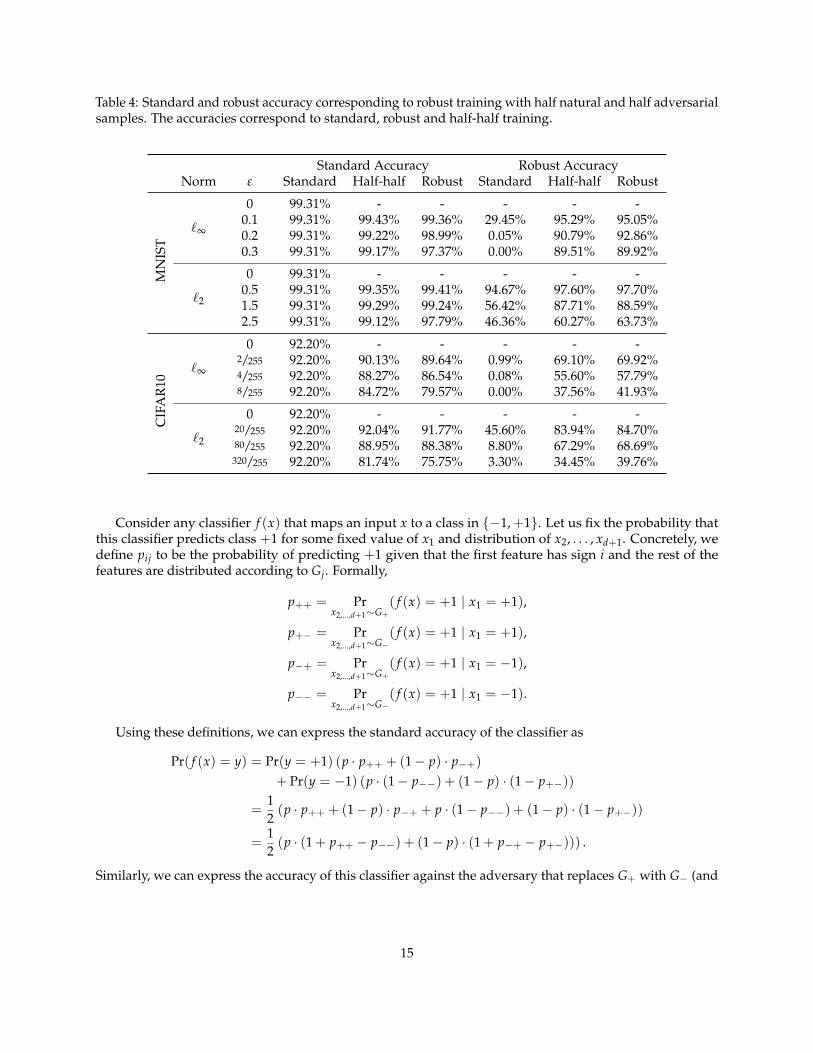
Table 4: Standard and robust accuracy corresponding to robust training with half natural and half adversarialsamples. The accuracies correspond to standard, robust and half-half training.
Standard Accuracy Robust AccuracyNorm ε Standard Half-half Robust Standard Half-half Robust
MN
IST
`∞
0 99.31% - - - - -0.1 99.31% 99.43% 99.36% 29.45% 95.29% 95.05%0.2 99.31% 99.22% 98.99% 0.05% 90.79% 92.86%0.3 99.31% 99.17% 97.37% 0.00% 89.51% 89.92%
`2
0 99.31% - - - - -0.5 99.31% 99.35% 99.41% 94.67% 97.60% 97.70%1.5 99.31% 99.29% 99.24% 56.42% 87.71% 88.59%2.5 99.31% 99.12% 97.79% 46.36% 60.27% 63.73%
CIF
AR
10
`∞
0 92.20% - - - - -2/255 92.20% 90.13% 89.64% 0.99% 69.10% 69.92%4/255 92.20% 88.27% 86.54% 0.08% 55.60% 57.79%8/255 92.20% 84.72% 79.57% 0.00% 37.56% 41.93%
`2
0 92.20% - - - - -20/255 92.20% 92.04% 91.77% 45.60% 83.94% 84.70%80/255 92.20% 88.95% 88.38% 8.80% 67.29% 68.69%
320/255 92.20% 81.74% 75.75% 3.30% 34.45% 39.76%
Consider any classifier f (x) that maps an input x to a class in {−1,+1}. Let us fix the probability thatthis classifier predicts class +1 for some fixed value of x1 and distribution of x2, . . . , xd+1. Concretely, wedefine pij to be the probability of predicting +1 given that the first feature has sign i and the rest of thefeatures are distributed according to Gj. Formally,
p++ = Prx2,...,d+1∼G+
( f (x) = +1 | x1 = +1),
p+− = Prx2,...,d+1∼G−
( f (x) = +1 | x1 = +1),
p−+ = Prx2,...,d+1∼G+
( f (x) = +1 | x1 = −1),
p−− = Prx2,...,d+1∼G−
( f (x) = +1 | x1 = −1).
Using these definitions, we can express the standard accuracy of the classifier as
Pr( f (x) = y) = Pr(y = +1) (p · p++ + (1− p) · p−+)+ Pr(y = −1) (p · (1− p−−) + (1− p) · (1− p+−))
=12(p · p++ + (1− p) · p−+ + p · (1− p−−) + (1− p) · (1− p+−))
=12(p · (1 + p++ − p−−) + (1− p) · (1 + p−+ − p+−))) .
Similarly, we can express the accuracy of this classifier against the adversary that replaces G+ with G− (and
15
vice-versa) as
Pr( f (xadv) = y) = Pr(y = +1) (p · p+− + (1− p) · p−−)+ Pr(y = −1) (p · (1− p−+) + (1− p) · (1− p++))
=12(p · p+− + (1− p) · p−− + p · (1− p−+) + (1− p) · (1− p++))
=12(p · (1 + p+− − p−+) + (1− p) · (1 + p−− − p++))) .
For convenience we will define a = 1− p++ + p−− and b = 1− p−+ + p+−. Then we can rewrite
standard accuracy :12(p(2− a) + (1− p)(2− b))
= 1− 12(pa + (1− p)b),
adversarial accuracy :12((1− p)a + pb).
We are assuming that the standard accuracy of the classifier is at least 1− δ for some small δ. This impliesthat
1− 12(pa + (1− p)b) ≥ 1− δ =⇒ pa + (1− p)b ≤ 2δ.
Since pij are probabilities, we can guarantee that a ≥ 0. Moreover, since p ≥ 0.5, we have p/(1− p) ≥ 1. Weuse these to upper bound the adversarial accuracy by
12((1− p)a + pb) ≤ 1
2
((1− p)
p2
(1− p)2 a + pb)
=p
2(1− p)(pa + (1− p)b)
≤ p1− p
δ.
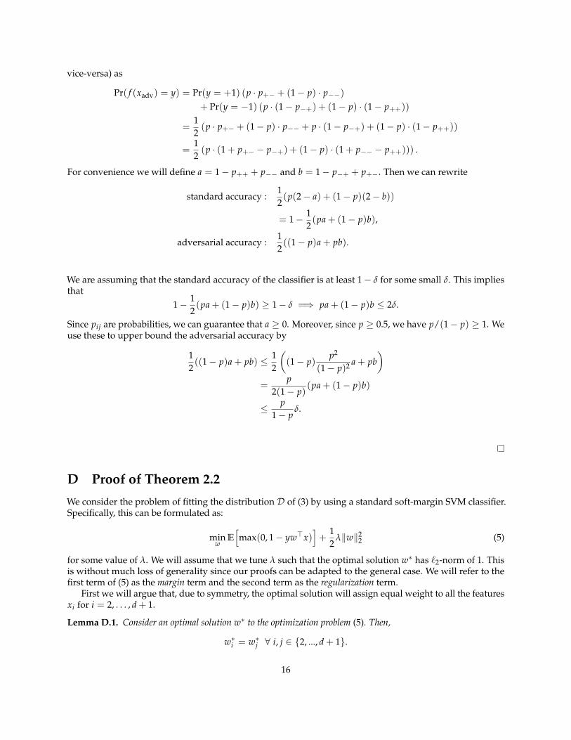
D Proof of Theorem 2.2
We consider the problem of fitting the distribution D of (3) by using a standard soft-margin SVM classifier.Specifically, this can be formulated as:
minw
E[max(0, 1− yw>x)
]+
12
λ‖w‖22 (5)
for some value of λ. We will assume that we tune λ such that the optimal solution w∗ has `2-norm of 1. Thisis without much loss of generality since our proofs can be adapted to the general case. We will refer to thefirst term of (5) as the margin term and the second term as the regularization term.
First we will argue that, due to symmetry, the optimal solution will assign equal weight to all the featuresxi for i = 2, . . . , d + 1.
Lemma D.1. Consider an optimal solution w∗ to the optimization problem (5). Then,
w∗i = w∗j ∀ i, j ∈ {2, ..., d + 1}.
16

Proof. Assume that ∃ i, j ∈ {2, ..., d + 1} such that w∗i 6= w∗j . Since the distribution of xi and xj are identical,we can swap the value of wi and wj, to get an alternative set of parameters w that has the same loss functionvalue (wj = wi, wi = wj, wk = wk for k 6= i, j).
Moreover, since the margin term of the loss is convex in w, using Jensen’s inequality, we get that averagingw∗ and w will not increase the value of that margin term. Note, however, that ‖w∗+w
2 ‖2 < ‖w∗‖2, hence theregularization loss is strictly smaller for the average point. This contradicts the optimality of w∗.
Since every optimal solution will assign equal weight to all xi for k ≥ 2, we can replace these features bytheir sum (and divide by
√d for convenience). We will define
z =1√d
d+1
∑i=2
xi,
which, by the properties of the normal distribution, is distributed as
z ∼ N (yη√
d, 1).
By assigning a weight of v to that combined feature the optimal solutions can be parametrized as
w>x = w1x1 + vz,
where the regularization term of the loss is λ(w21 + v2)/2.
Recall that our chosen value of η is 4/√
d, which implies that the contribution of vz is distributed normallywith mean 4yv and variance v2. By the concentration of the normal distribution, the probability of vz beinglarger than v is large. We will use this fact to show that the optimal classifier will assign on v at least as muchweight as it assigns on w1.
Lemma D.2. Consider the optimal solution (w∗1 , v∗) of the problem (5). Then
v∗ ≥ 1√2
.
Proof. Assume for the sake of contradiction that v∗ < 1/√
2. Then, with probability at least 1− p, the firstfeature predicts the wrong label and without enough weight, the remaining features cannot compensate forit. Concretely,
E[max(0, 1− yw>x)] ≥ (1− p) E[max
(0, 1 + w1 −N
(4v, v2
))]≥ (1− p) E
[max
(0, 1 +
1√2−N
(4√2
,12
))]> (1− p) · 0.016.
We will now show that a solution that assigns zero weight on the first feature (v = 1 and w1 = 0),achieves a better margin loss.
E[max(0, 1− yw>x)] = E [max (0, 1−N (4, 1))]< 0.0004.
Hence, as long as p ≤ 0.975, this solution has a smaller margin loss than the original solution. Since bothsolutions have the same norm, the solution that assigns weight only on v is better than the original solution(w∗1 , v∗), contradicting its optimality.
We have established that the learned classifier will assign more weight to v than w1. Since z will be atleast y with large probability, we will show that the behavior of the classifier depends entirely on z.
17

Lemma D.3. The standard accuracy of the soft-margin SVM learned for problem (5) is at least 99%.
Proof. By Lemma D.2, the classifier predicts the sign of w1x1 + vz where vz ∼ N (4yv, v2) and v ≥ 1/√
2.Hence with probability at least 99%, vzy > 1/
√2 ≥ w1 and thus the predicted class is y (the correct class)
independent of x1.
We can utilize the same argument to show that an adversary that changes the distribution of z hasessentially full control over the classifier prediction.
Lemma D.4. The adversarial accuracy of the soft-margin SVM learned for (5) is at most 1% against an `∞-boundedadversary of ε = 2η.
Proof. Observe that the adversary can shift each feature xi towards y by 2η. This will cause z to be distributedas
zadv ∼ N (−yη√
d, 1).
Therefore with probability at least 99%, vyz < −y ≤ −w1 and the predicted class will be −y (wrong class)independent of x1.
It remains to show that adversarial training for this classification task with ε > 2η will results in aclassifier that has relies solely on the first feature.
Lemma D.5. Minimizing the adversarial variant of the loss (5) results in a classifier that assigns 0 weight to featuresxi for i ≥ 2.
Proof. The optimization problem that adversarial training solves is
minw
max‖δ‖∞≤ε
E[max(0, 1− yw>(x + δ))
]+
12
λ‖w‖22,
which is equivalent to
minw
E[max(0, 1− yw>x + ε‖w‖1)
]+
12
λ‖w‖22.
Consider any optimal solution w for which wi > 0 for some i > 2. The contribution of terms depending onwi to 1− yw>x + ε‖w‖1 is a normally-distributed random variable with mean 2η − ε ≤ 0. Since the mean isnon-positive, setting wi to zero can only decrease the margin term of the loss. At the same time, setting wi tozero strictly decreases the regularization term, contradicting the optimality of w.
Clearly, such a classifier will have standard and adversarial accuracy of p against any ε < 1 since such avalue of ε is not sufficient to change the sign of the first feature. This concludes the proof of the theorem.
E Robustness-accuracy trade-off: An empirical examination
Our theoretical analysis shows that there is an inherent tension between standard accuracy and adversarialrobustness. At the core of this trade-off is the concept of robust and non-robust features. We now investigatewhether this notion arises experimentally by studying a dataset that is amenable to linear classifiers,MNIST (LeCun, 1998) (details in Appendix A).
Recall the goal of standard classification for linear classifiers is to predict accurately, i.e. y = sign(w>x).Hence the correlation of a feature i with the true label, computed as |E[yxi]|, quantifies how useful thisfeature is for classification. In the adversarial setting, against an ε `∞-bounded adversary we need to ensurethat y = sign(w>x− εy‖w‖1). In that case we roughly expect a feature i to be helpful if |E[yxi]| ≥ ε.
This calculation suggests that in the adversarial setting, there is an implicit threshold on feature corre-lations imposed by the threat model (the perturbation allowed to the adversary). While standard modelsmay utilize all features with non-zero correlations, a robust model cannot rely on features with correlation
18

Stan
dard
Model WeightsAd
vers
aria
l
(a)
100 101 102 103
#Feature
0.00
0.05
0.10
0.15
0.20
0.25
0.30
Wei
ght
(b)
Correlation w Label
Feature ThresholdStandard TrainingAdversarial Training
100 101 102 103
Fraction of features chosen
20
40
60
80
100
Accu
racy
(%)
(c)
Standard (train)Standard (test)w Robust Features (train)w Robust Features (test)Adversarial Training (test)
Figure 5: Analysis of linear classifier trained on a binary MNIST task (5 vs. 7). (Details in Appendix Table 5.)(a) Visualization of network weights per input feature. (b) Comparison of feature-label correlation to theweight assigned to the feature by each network. Adversarially trained networks put weights only on asmall number of strongly-correlated or “robust” features. (c) Performance of a model trained using standardtraining only on the most robust features. Specifically, we sort features based on decreasing correlation withthe label and train using only the most correlated ones. Beyond a certain threshold, we observe that as morenon-robust or (weakly correlated) features are available to the model, the standard accuracy increases at thecost of robustness.
below this threshold. In Figure 5(b), we visualize the correlation of each pixel (feature) in the MNIST datasetalong with the learned weights of the standard and robust classifiers. As expected, we see that the standardclassifier assigns weights even to weakly-correlated pixels so as to maximize prediction confidence. On theother hand, the robust classifier does not assign any weight below a certain correlation threshold which isdictated by the adversary’s strength (ε) (Figures 5(a, b))
Interestingly, the standard model assigns non-zero weight even to very weakly correlated pixels (Fig-ure 5(a)). In settings with finite training data, such non-robust features could arise from noise. (For instance,in N tosses of an unbiased coin, the expected imbalance between heads and tails is O(
√N) with high
probability.) A standard classifier would try to take advantage of even this “hallucinated” information byassigning non-zero weights to these features.
E.1 An alternative path to robustness?
The analysis above highlights an interesting trade-off between the predictive power of a feature and itsvulnerability to adversarial perturbations. This brings forth the question – Could we use these insightsto train robust classifiers with standard methods (i.e. without performing adversarial training)? As a firststep, we train a (standard) linear classifier on MNIST utilizing input features (pixels) that lie above a givencorrelation threshold (see Figure 5(c)). As expected, as more non robust features are incorporated in training,the standard accuracy increases at the cost of robustness. Further, we observe that a standard classifiertrained in this manner using few robust features attains better robustness than even adversarial training.This results suggest a more direct (and potentially better) method of training robust networks in certainsettings.
19
F Additional related work
Fawzi et al. (2016) derive parameter-dependent bounds on the robustness of any fixed classifier, while Wanget al. (2018) analyze the adversarial robustness of nearest neighbor classifiers. Our results focus on thestatistical setting itself and provide lower bounds for all classifiers learned in this setting.
Schmidt et al. (2018) study the generalization aspect of adversarially robustness. They show that thenumber of samples needed to achieve adversarially robust generalization is polynomially larger in thedimension than the number of samples needed to ensure standard generalization. However, in the limit ofinfinite data, one can learn classifiers that are both robust and accurate and thus the trade-off we study doesnot manifest.
Gilmer et al. (2018) demonstrate a setting where even a small amount of standard error implies that mostpoints provably have a misclassified point close to them. In this setting, achieving perfect standard accuracy(easily achieved by a simple classifier) is sufficient to achieve perfect adversarial robustness. In contrast, ourwork focuses on a setting where adversarial training (provably) matters and there exists a trade-off betweenstandard and adversarial accuracy.
Xu & Mannor (2012) explore the connection between robustness and generalization, showing that, in acertain sense, robustness can imply generalization. This direction is orthogonal to our, since we work in thelimit of infinite data, optimizing the distributional loss directly.
Fawzi et al. (2018a) prove lower bounds on the robustness of any classifier based on certain generativeassumptions. Since these bounds apply to all classifiers, independent of architecture and training procedure,they fail to capture the situation we face in practice where robust optimization can significantly improve theadversarial robustness of standard classifiers (Madry et al., 2018; Wong & Kolter, 2018; Raghunathan et al.,2018; Sinha et al., 2018).
A recent work (Bubeck et al., 2018) turns out to (implicitly) rely on the distinction between robust andnon-robust features in constructing a distribution for which adversarial robustness is hard from a different,computational point of view.
Goodfellow et al. (2015) observed that adversarial training results in feature weights that depend onfewer input features (similar to Figure 5(a)). Additionally, it has been observed that for naturally trained RBFclassifiers on MNIST, targeted adversarial attacks resemble images of the target class (Goodfellow, 2015).
Su et al. (2018) empirically observe a similar trade-off between the accuracy and robustness of standardmodels across different deep architectures on ImageNet.
20

G Omitted figures
Table 5: Comparison of performance of linear classifiers trained on a binary MNIST dataset with standardand adversarial training. The performance of both models is evaluated in terms of standard and adversarialaccuracy. Adversarial accuracy refers to the percentage of examples that are correctly classified after beingperturbed by the adversary. Here, we use an `∞ threat model with ε = 0.20 (with images scaled to havecoordinates in the range [0, 1]).
Standard Accuracy (%) Adversarial Accuracy (%) ‖w‖1Train Test Train Test
Standard Training 98.38 92.10 13.69 14.95 41.08Adversarial Training 94.05 70.05 76.05 74.65 13.69
103 104
# Training Samples
94
95
96
97
98
99
Stan
dard
Acc
urac
y (%
)
-trained
train =00.10.20.3
(a) MNIST
102 103 104
# Training Samples
40
50
60
70
80
90
Stan
dard
Acc
urac
y (%
)
-trained
train =02/2554/2558/255
(b) CIFAR-10
103 104 105
# Training Samples20
30
40
50
60
70
80
90
Stan
dard
Acc
urac
y (%
)
-trained
train =00.0125
(c) Restricted ImageNet
Figure 6: Comparison of standard accuracies of models trained against an `∞-bounded adversary as afunction of the size of the training dataset. We observe that in the low-data regime, adversarial traininghas an effect similar to data augmentation and helps with generalization in certain cases (particularly onMNIST). However, in the limit of sufficient training data, we see that the standard accuracy of robust modelsis less than that of the standard model (εtrain = 0), which supports the theoretical analysis in Section 2.1.
0.00 0.05 0.10 0.15 0.20 0.25 0.30 0.3594
97
100
-trai
ning
Test
Acc
urac
y (%
)
MNIST
0.000 0.005 0.010 0.015 0.020 0.025 0.03050
75
100CIFAR-10
0.00 0.02 0.04 0.06 0.08 0.100
50
100Restricted ImageNet
0.0 0.5 1.0 1.5 2.0 2.5
Train
94
97
100
2-tra
inin
g
0.0 0.2 0.4 0.6 0.8 1.0 1.2
Train
50
75
100
0.0 0.2 0.4 0.6 0.8 1.0
Train
85
100
Figure 7: Standard test accuracy of adversarially trained classifiers. The adversary used during training isconstrained within some `p-ball of radius εtrain (details in Appendix A). We observe a consistent decrease inaccuracy as the strength of the adversary increases.
21

5
Orig
inal
9 7 3 4 9 6 6 5
3
Stan
dard
4 9 8 7 7 5 4 6
5
-trai
ned
9 7 8 4 9 6 6 5
3
2-tra
ined
4 7 8 4 7 5 6 5
(a) MNIST
cat
Orig
inal
ship ship airplane frog frog automobile frog cat
bird
Stan
dard
automobile bird bird bird bird frog bird frog
frog
-trai
ned
automobile automobile bird deer horse truck deer bird
frog
2-tra
ined
automobile automobile ship deer truck cat cat deer
(b) CIFAR-10
(c) Restricted ImageNet
Figure 8: Large-ε adversarial examples, bounded in `∞-norm, similar to those in Figure 3.
22

5
Orig
inal
9 7 3 4 9 6 6 5
3
Stan
dard
4 2 8 5 7 5 4 6
5
-trai
ned
4 7 8 4 7 5 5 5
3
2-tra
ined
4 2 5 9 7 5 4 8
(a) MNIST
cat
Orig
inal
ship ship airplane frog frog automobile frog cat
frog
Stan
dard
bird bird bird deer bird truck bird bird
frog
-trai
ned
airplane truck deer deer deer dog deer frog
bird
2-tra
ined
automobile automobile ship deer truck cat deer frog
(b) CIFAR-10
(c) Restricted ImageNet
Figure 9: Large-ε adversarial examples, bounded in `2-norm, similar to those in Figure 3.
23

Orig
inal
9 6 6 5 4 0 7 4 0 1
Stan
dard
-trai
ned
2-tra
ined
(a) MNIST
Orig
inal
dog horse truck ship dog horse ship frog horse airplane
Stan
dard
-trai
ned
2-tra
ined
(b) CIFAR-10
(c) Restricted ImageNet
Figure 10: Visualization of the gradient of the loss with respect to input features (pixels) for standard andadversarially trained networks for 10 randomly chosen samples, similar to those in Figure 2. Gradientsare significantly more interpretable for adversarially trained networks – they align well with perceptuallyrelevant features. For MNIST, blue and red pixels denote positive and negative gradient regions respectively.For CIFAR10 and Restricted ImageNet we clip pixel to 3 standard deviations and scale to [0, 1].
24