J Glob OptimDOI 10.1007/s10898-009-9496-x

Robust optimization with simulated annealing

Dimitris Bertsimas · Omid Nohadani

Received: 17 March 2009 / Accepted: 11 November 2009© Springer Science+Business Media, LLC. 2009

Abstract Complex systems can be optimized to improve the performance with respectto desired functionalities. An optimized solution, however, can become suboptimal or eveninfeasible, when errors in implementation or input data are encountered. We report on a robustsimulated annealing algorithm that does not require any knowledge of the problems structure.This is necessary in many engineering applications where solutions are often not explicitlyknown and have to be obtained by numerical simulations. While this nonconvex and globaloptimization method improves the performance as well as the robustness, it also warrants fora global optimum which is robust against data and implementation uncertainties. We dem-onstrate it on a polynomial optimization problem and on a high-dimensional and complexnanophotonic engineering problem and show significant improvements in efficiency as wellas in actual optimality.

Keywords Robust optimization · Simulated annealing · Global optimization · Nonconvexoptimization

1 Introduction

Optimization has had a distinguished history in engineering and industrial design. Mostapproaches, however, assume that the input parameters are precisely known and that theimplementation does not suffer any errors. To accommodate these sources of errors, sensi-tivity analysis techniques were developed which find solutions that are least sensitive amonga larger set of optima. However, these methods do not provide designs that are intrinsicallyrobust against errors.

D. Bertsimas · O. Nohadani (B)Sloan School of Management and the Operations Research Center, Massachusetts Institute of Technology,Cambridge, MA 02139, USAe-mail: nohadani@mit.edu

D. Bertsimase-mail: dbertsim@mit.edu

123

J Glob Optim

There has been evidence illustrating that if errors (in implementation or estimation ofparameters) are not taken into account during the design process, the actual phenomenon cancompletely disappear. A prime example is optimizing the truss design for suspension bridges.The Tacoma Narrows bridge was the first of its kind to be optimized to divert the wind aboveand below the roadbed [1]. Only a few months after its opening in 1940, it collapsed due tomoderate winds which caused twisting vibrational modes. In another example, Ben-Tal andNemirovski demonstrated that only 5% errors can entirely destroy the radiation characteris-tics of an otherwise optimized phased locked and impedance matched array of antenna [2].Therefore, taking errors into account during the optimization process is a first order effect.

These considerations have motivated the field of robust optimization. Recent works havebeen devoted to problems with convex objectives and constraints (e.g. linear) [3–5]. Theseworks have shown that a convex optimization problem with parameter uncertainty can betransformed to another convex optimization problem. This transformation can be either exactor through a relaxation. However, the final problem can be more complex or can have a sig-nificantly larger number of constraints. Despite significant advancements, all these resultsare limited to convex problems.

Modern engineering design has objectives and constraints that are not explicitly given.Moreover, solutions are often obtained through numerical simulations. This means that nointernal structure can be exploited. The challenge, thus, lies in robustly designing engineeredand engineering systems which are described through simulations and are exposed to errors.

More recently, local search methods have been expanded to robust optimization of sim-ulated-based problems [6–8]. They entail finding descent directions and iteratively takingsteps along these directions to optimize the robustness, i.e., reducing the worst-case cost. Asecond order cone problem was solved to determine a direction that makes the largest angleto all worst-case neighbors that were found to deviate the most from the desired solution.The number of regarded worst-case scenarios and the dimensionality determined the compu-tational efficiency of these algorithms [8]. These approaches, however, provided only localrobust optima.

Here, we present a more generic method, that is independent of the problem structure and,thus, is not restricted to dimensionality or other topological features. In fact, it only requiresa black-box that provides the function evaluation and the derivative for a given design. More-over, we show that this technique can provide a global robust optimum at computationallyreasonable costs. We showcase its performance on a 100-dimensional optimization problemin nanophotonic design, that has a highly nonconvex cost function as well as nonconvexsearch space.

2 Method

In general, to measure the deviations between the desired and current performance of a designx, a cost function f is defined. For the purpose of generality, we do not impose any assump-tion of the structure on f , i.e., f can be nonconvex or simply given through a numericalsimulation. The nominal optimization aims to minimize f . There are numerous techniquesto achieve this goal for which we refer to the standard literature [9–11]. In real-world prob-lems, the design variables x are subject to errors �x. Therefore, possible designs are regardedto reside within an uncertainty set

U = {�x ∈ Rn | ‖�x‖ ≤ �}, (1)

123

J Glob Optim

Fig. 1 2D-Sketch: Robustness is determined by worst-case costs within the uncertainty set (discs) of a design(point in x–y plane). Robust optimization seeks to place the lowest disc (red), even lower than the nominaloptimum (yellow)

where � denotes the size of U , determined by empirical error bars. While our approachapplies to other norms ‖�x‖p ≤ � in (1) (p being a positive integer, including p = ∞),we present the case of p = 2. To find a design that is robust against all possible errors in U ,the most conservative approach is to find worst-case scenarios g(x) = max�x∈U f (x +�x)

and seek to minimize them by modifying the design appropriately. This robust optimizationproblem can be expressed through

minx

g(x) ≡ minx

max�x∈U f (x + �x). (2)

Since f is nonconvex and possibly not given in an analytically closed form, the inner max-imization problem will be nonconvex and without a closed form as well. In our method, itssolution is found using local searches within the uncertainty set of the design (see Fig. 1).These searches, such as gradient ascent sequences, identify a potentially discrete set M(x)

of “bad neighbors” x̂ which have the highest costs in U . Once M(x) is assembled for a givendesign x, the robust optimization method seeks to iteratively update x in order to excludethe elements of M(x) and consequently finds designs that have lower worst-case neighbors,thus improve robustness. In earlier works, the robust local method was used to find a localrobust optimum [6, 8].

To find the global robust minimum, we introduce the method of robust simulated annealing(RSA). In a pioneering work, Kirkpatrick et al. introduced the method of simulated anneal-ing for discrete optimization problems [12]. Relying on one of the early works in scientificcomputing by Metropolis et al. [13], they replaced the energy of an ensemble by the cost

123

J Glob Optim

function of a configuration and showed the connection between optimizing a multivariatefunction and the behavior of many-body systems with a large degree of freedom in thermalequilibrium. Motivated by these works, we rewrite g(x) from Eq. 2 as follows

g(x) = limβ→∞ gβ(x) = lim

β→∞

⎧⎪⎨

⎪⎩

1

βlog

∫

x̂∈M(x)

eβf (x̂)d(x̂)

⎫⎪⎬

⎪⎭. (3)

We interpret the parameter β as the inverse temperature. We set β0 to be the highest cost in thebad neighbors set M(x) (see Eq. 4 below). In the RSA algorithm, gβ(x) is computed as a sumover the members of M(x) and the limβ→∞ in Eq. 3 is approximated by the largest availableβ. The RSA algorithm maximizes the robustness by iteratively minimizing the worst-casescenario of the current design xk as following:

RSA Algorithm:

Step 0. Initialization:

(i) Set iterate k = 0, acceptance number h = 0, and annealing index n = 0.(ii) Let x0 be the initial decision vector that is arbitrarily chosen.

(iii) Assemble M(x0) through a series of gradient ascent sequences withinU(x0) [8].

(iv) Compute the initial inverse temperature β0 according to

β0 = 1

maxx̂∈M(x0)

f (x̂). (4)

(v) Compute g(x0) ≡ gβ0(x0) according to Eq. 3.(vi) Determine the Boltzmann-weight W(xk) through

W(xk) = e−β g(xk). (5)

Step 1. Trial design:

(i) From a Gaussian probability distribution, randomly generate xtrial such that‖xtrial − xk‖2 ≤ �.

(ii) Assemble M(xtrial) within U(xtrial) as above.(iii) Compute g(xtrial) ≡ gβ(xtrial) according to Eq. 3.(iv) Determine the Boltzmann-weight W(xtrial) as in Eq. 5.

Step 2. Compute the acceptance probability:

P(xk → xtrial) = min

(

1,W(xtrial)

W(xk)

)

(6)

from the respective weights to permit an update, corresponding to the Metropolisupdate scheme [13].

Step 3. Generate a random number R ∈ [0, 1]:(i) if P ≥ R: xtrial is accepted

(a) k = k + 1 and xk+1 = xtrial

(b) h = h + 1, and(A) if (h mod 100) �= 0, then g(xk+1)=g(xtrial) and W(xk+1)=

W(xtrial).

123

J Glob Optim

(B) else n = n + 1 and update the inverse temperature via

βn = β0ecn, (7)

with c = 1 + ε. Recompute g(xk+1) and W(xk+1) with theupdated β.

(c) Back to Step 1 and iterate.(ii) if P < R: xtrial is rejected. Back to Step 1 and reiterate.

Note that in this algorithm, there are 2 iteration indices: n denotes the annealing index,which increases whenever the inverse temperature is updated, and k denotes the trial indexwithin each annealing iterate in order to find a more robust trial decision xtrial at the sameinverse temperature.

Theorem 1 Suppose that an arbitrary cost function f (x) with a bounded set of minimumpoints has a global robust optimum. Then the RSA Algorithm converges to the global optimumof the robust optimization problem (2), if all designs x are accessible with equal probabilityas n → ∞.

Proof Geman and Geman have shown that a generic simulated annealing algorithm con-verges to a global optimum, if β is selected to be not faster than βn = ln(n)/β0 and if allaccessible states are equally probable for n → ∞ [14].

The first condition is satisfied by the choice of the annealing schedule in Eq. 7. For thesecond condition, let H(x) be the probability density of the randomly generated designs xtrial.In order to show that any design x in the D-dimensional configuration space can be sampledinfinitely often during the annealing time, we have to show that the probability of not visitingx during the annealing time vanishes. In other words, we have to show that

∞∏

n=0

(1 − Hn(x)) = 0, (8)

which can be expressed as

∞∑

n=0

Hn(x) = ∞. (9)

Ingber et al. [15] have shown that the functional form of random generators for Gaussian-Markovian based systems, like the one we employed to generate xtrial, is given by

H(x) =(

β

2π

)D2 · e− β

2 �x2, (10)

where 1/β is a measure of the fluctuations (standard deviation) and �x is difference betweenthe current and the previous design. As the algorithm progresses, β is updated. Thus, theEq. 10 can be expressed as

Hn(x) =(

β0ecn

2π

)D2 · e− β0ecn

2 �x2 ≥ e− ln(n). (11)

Now, we can insert Eq. 11 into Eq. 9 and obtain

∞∑

n=0

Hn(x) ≥∞∑

n=0

e− ln(n) =∞∑

n=0

1

n= ∞. (12)

123

J Glob Optim

Therefore, as n → ∞, all designs can be generated infinitely often. Moreover, the Metropolisweights are chosen such that the detailed balance condition

P(x → x′) · W(x) = P(x′ → x) · W(x′), (13)

is satisfied which warrants for an equal probability that all states are accessible in the searchspace. Therefore, we can conclude that the local search based RSA algorithm converges toa global optimum as n → ∞. �

Note that the definition of the robustness in Eq. 3 contains β which varies throughout theannealing process. However, this does not affect the probability density H(x) of the designs.Moreover, within each iteration of the RSA algorithm (and in fact over 100 acceptances),β is constant and acts only as a local renormalization factor. Even when β is updated inStep 3-ii-B, g(xk) and W(xk) are recomputed so that the current and the next trial design arecompared at the same constant β ensuring a constant local probability density. Therefore,this enhancement to the weighting in g(x) does not affect the convergence criteria of theRSA algorithm. Furthermore, the convergence behavior of RSA is similar to that of adaptivesimulated annealing, since their cores are comparable. However, since the convergence rateis highly dependent on the underlying problem and our aim to provide the general foundationof RSA, we consider this discussion outside the scope of this work.

We demonstrate the performance of the RSA algorithm by applying it to two differentoptimization problems. The first application is a robust polynomial optimization problem thatis intended to serve as a demonstration of the main features of RSA as well as its capabilityof providing a robust global optimum. This is a simple enough problem in which we cancalculate the robust global optimum. The second application is on the robust optimization inengineering and is of direct relevance to nanophotonics and nanotechnology design, wheresmall uncertainties may result in complete failure of an otherwise optimized design. Thisproblem is high-dimensional, highly non-linear and its solution is not known explicitly, thususeful as a prototype for modern engineering design problems. This application is intendedto demonstrate the performance of the RSA algorithm in a high-dimensional search space aswell as its efficiency of providing the robust solution.

3 Application in polynomial optimization

For the sake of better demonstration of the RSA algorithm, we employ a two dimensionalpolynomial problem. We define a nonconvex polynomial function

f (x, y) = 2x6 − 12.2x5 + 21.2x4 + 6.2x − 6.4x3

− 4.7x2 + y6 − 11y5 + 43.3y4 − 10y

− 74.8y3 + 56.9y2 − 4.1xy − 0.1y2x2

+ 0.4y2x + 0.4x2y. (14)

The implementation errors are bound as � = (�x,�y) by ‖�‖2 ≤ 0.5. Therefore, therobust optimization problem can be posed as

minx,y

g(x, y) ≡ minx,y

max‖�‖2≤0.5f (x + �x, y + �y). (15)

We need to stress that even though this problem is only two-dimensional, it is already adifficult problem. Henrion and Lasserre successfully introduced relaxation methods to solve

123

J Glob Optim

polynomial optimization problems [16, 17]. Applying the same technique to Problem (15),however, leads to polynomial semidefinite programs (SDP) which have the form of

minx,y

h(x, y)

s.t. A(x, y) � 0.(16)

Note that the entries of the semidefinite constraint are assembled by multivariate polynomialsAij . In order to solve this problem approximately, we need to convert it into a significantlylarger SDP. More importantly, the size of the SDP grows with the size of the original problem,the maximum degree of the polynomials, and the number of variables. Because of this, it isevident that polynomial SDPs are not widely used in practice [18].

The nominal cost off (x, y)has multiple local minima and a global minimum at (x∗, y∗) =(2.8, 4.0), where f (x∗, y∗) = −20.8. We determined the global minimum by using theGloptipoly software as discussed in Reference [16] and verified using multiple gradientdescents. We evaluated the worst-case cost function g(x, y) by enumerating the nominalcosts of neighbors using a fine discrete mesh. The Contour plot in Fig. 2 illustrates theworst-case cost surface and suggests that g(x, y) has multiple local minima.

We applied the Robust Simulated Annealing algorithm to this polynomial problem usingarbitrary initial designs (x, y). Figure 2 shows one exemplary run and demonstrates the con-vergence towards to robust global minimum. The same global optimum is found when startingfrom other arbitrary initial points. The algorithm decreases the worst-case cost significantlywhile increasing the nominal cost slightly, which is the “price of robustness”. A much lowernumber of iterations is required when starting from a point that is not in the immediate prox-imity of a local (robust or nominal) minimum. At the termination point, the last configurationis surrounded by neighbors that have higher worst-case costs. In fact, detailed analysis of thedistribution of bad neighbors at the termination showed that they lie on the boundary of theuncertainty set. Any additional trial configuration will lead to a vanishing update probability

Fig. 2 2D-Sketch: Contour plot of worst-case cost function g(x, y). The path of the progress of the RobustSimulated Annealing algorithm is shown with red lines as it starts at an arbitrary initial point and convergestowards to robust global minimum

123

J Glob Optim

and, thus, will be rejected. The surface plot also confirms that the solution is indeed the truerobust global minimum.

4 Application in nanophotonic optimization

In the second application, we demonstrate the efficiency and the performance of the RSAalgorithm by applying it to a prototype electromagnetic problem, as it occurs in nanophotonicengineering. A plethora of unique characteristics in photonic crystals identified them as primecandidates for unconventional materials in controlling and manipulating electromagneticfield propagation [19]. Their peculiar functionalities are based on diffraction phenomena,which require periodic structures. Upon breaking the spatial symmetry, additional degreesof freedom are revealed which allow for additional functionality and higher levels of con-trol. Geremia et al. broke this symmetry by diluting sites and optimizing the location of themissing scattering sites [20]. However, due to the periodicity requirement of these crystals,additional degrees of freedom and, hence, their benefit remained restricted. More recently,Seliger et al. performed unbiased gradient-based optimizations on the spatial distribution of alarge number of dielectric cylinders [21]. The reported aperiodic structure matched a desiredtarget function up to 95%.

When implemented in the real-world, however, the performance of many of these designssubstantially deviates from the theoretical prediction. A key source of this deviation liesin the presence of uncontrollable implementation errors, such as incorrect positioning anderroneous shape of scatterers. Since nanophotonic structures exploit nonlinear features, theyare highly susceptive to small perturbations. Therefore, a robustly optimized design warrantsthe desired performance and sustains errors.

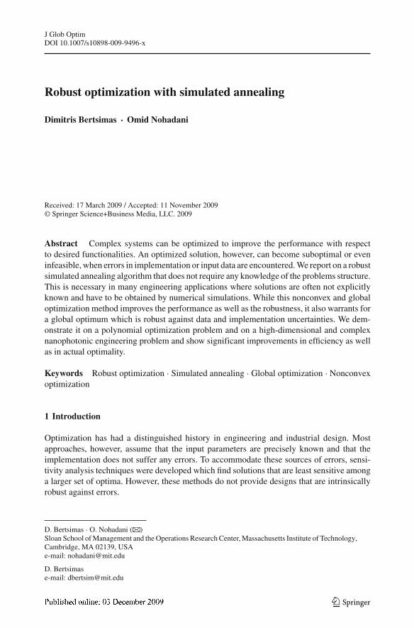
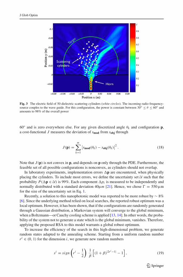
We demonstrate this by applying the RSA method to an inverse design problem, that seeksto match the performance of 50 dielectric cylinders to a desired target function by varyingthe position of these scattering centers. In the following, we summarize the essentials of thephysical model for the sake of completeness and refer for more details to References [6, 21].The model is based on a two-dimensional Helmholtz equation for dielectric scatterers, whichare lossless and non-magnetic. Therefore, this approach scales with frequency and allowsto probe nanophotonic designs. The wave propagation is strictly two-dimensional, sincethe domain is bound by two metallic plates separated by less than half the incoming wavelength. Figure 3 illustrates the setup of the domain along with the corresponding electric fieldstrength. To conform with the laboratory experiment of Seliger et al. [21], we describe theelectric field Ez through the partial differential equation (PDE)

(∂x(µ−1ry

∂x) + ∂y(µ−1rx

∂y))Ez − ω20µ0ε0εrzEz = 0, (17)

where µr is the relative and µ0 the vacuum permeability and εr denotes the relative andε0 the vacuum permittivity. Note, that in the experimental measurements, the frequency isfixed to f = 37.5 GHz and only stationary solutions of the Maxwell equations are sought,taking the boundary conditions into account. We compute the field values using the finite-difference representation of the PDE and solve a linear equation system. The power alongthe target surface for an incident angle θ is interpolated using the nearest four mesh pointsand their standard Gaussian weights W(θ) as smod(θ) = W(θ)

2 · diag(Ez) · Ez . The accu-racy of this numerical model has been verified by actual laboratory experiments of identicalconfigurations [6, 21].

The nominal optimization problem seeks to match the power profile along the detectionsurface to a top-hat target function sobj, which has a constant maximum between 30◦ ≤ θ ≤

123

J Glob Optim

Fig. 3 The electric field of 50 dielectric scattering cylinders (white circles). The incoming radio frequency-source couples to the wave guide. For this configuration, the power is constant between 30◦ ≤ θ ≤ 60◦ andamounts to 98% of the overall power

60◦ and is zero everywhere else. For any given discretized angle θk and configuration p,a cost-functional J measures the deviation of smod from sobj through

J (p) =m∑

k=1

∣∣smod(θk) − sobj(θk)

∣∣2

. (18)

Note that J (p) is not convex in p, and depends on p only through the PDE. Furthermore, thefeasible set of all possible configurations is nonconvex, as cylinders should not overlap.

In laboratory experiments, implementation errors �p are encountered, when physicallyplacing the cylinders. To include most errors, we define the uncertainty set U such that theprobability P(�p ∈ U) is 99%. Each component �pi is measured to be independently andnormally distributed with a standard deviation 40µm [21]. Hence, we chose � = 550 µmfor the size of the uncertainty set in Eq. 1.

Recently, a solution to this nanophotonic model was reported to be more robust by ∼ 8%[6]. Since the underlying method relied on local searches, the reported robust optimum was alocal optimum. However, it has been shown, that if the configurations are randomly generatedthrough a Gaussian distribution, a Markovian system will converge to the global minimum,when a Boltzmann—or Cauchy cooling scheme is applied [13, 14]. In other words, the proba-bility of the system not to generate a state which is the global minimum, vanishes. Therefore,applying the proposed RSA to this model warrants a global robust optimum.

To increase the efficiency of the search in this high-dimensional problem, we generaterandom states adapted to the annealing scheme. Starting from a uniform random numberri ∈ (0, 1) for the dimension i, we generate new random numbers

si = sign

(

ri − 1

2

)1

β

[(1 + β)|2ri−1| − 1

], (19)

123

J Glob Optim

0 200 400 600 800 1000

Iterations

0.02

0.03

0.04

0.05

Wor

st-c

ase

Cos

t

Re-annealingRe-annealing, Re-heating

(a)

0 200 400 600 800 1000

Iterations

0.02

0.03

0.04

0.05

Nom

inal

Cos

t

Re-annealingRe-annealing, Re-heating

(b)

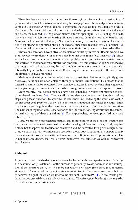
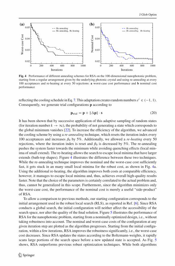
Fig. 4 Performance of different annealing schemes for RSA on the 100-dimensional nanophotonic problem,starting from a regular arrangement given by the underlying photonic crystal and using re-annealing at every100 acceptances and re-heating at every 50 rejections: a worst-case cost performance and b nominal costperformance

reflecting the cooling schedule in Eq. 7. This adaptation creates random numbers si ∈ (−1, 1).Consequently, we generate trial configurations p according to

ptrial = p + ‖�p‖ · s (20)

It has been shown that by successive application of this adaptive sampling of random states(for iteration number k → ∞), the probability of not generating a state which corresponds tothe global minimum vanishes [22]. To increase the efficiency of the algorithm, we advancedthe cooling scheme by using a re-annealing technique, which resets the iteration index every100 acceptances and increases β0 by 5%. Additionally, we allowed a re-heating every 50rejections, where the iteration index is reset and β0 is decreased by 5%. The re-annealingpushes the system faster towards the minimum while avoiding quenching effects (local min-ima of small extend). The re-heating allows the search to escape local minima that have largerextends (bath-top shapes). Figure 4 illustrates the difference between these two techniques.While the re-annealing technique improves the nominal and the worst-case cost sufficientlyfast, it gets stuck in an many small local minima for the robust cost, as shown in Fig. 4a.Using the additional re-heating, the algorithm improves both costs at comparable efficiency,however, it manages to escape local minima and, thus, achieves overall high-quality resultsfaster. Note that the choice of the parameters is certainly correlated to the actual problem and,thus, cannot be generalized in this scope. Furthermore, since the algorithm minimizes onlythe worst-case cost, the performance of the nominal cost is merely a useful “side-product”of RSA.

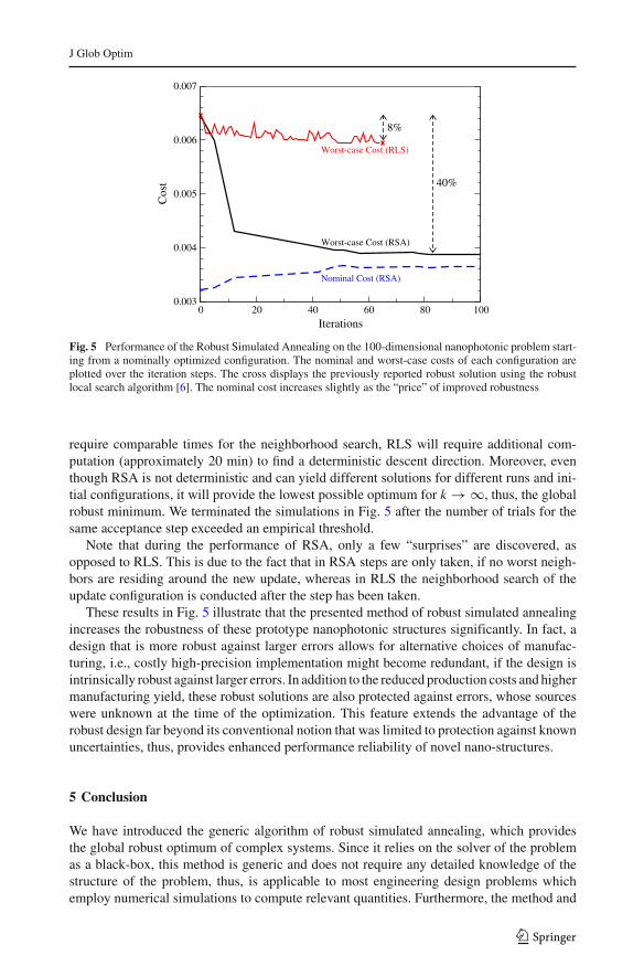
To allow a comparison to previous methods, our starting configuration corresponds to theinitial arrangement used in the robust local search (RLS), as reported in Ref. [6]. Since RSAconducts a global search, the initial configuration will neither affect the accessibility of thesearch space, nor alter the quality of the final solution. Figure 5 illustrates the performance ofRSA for the nanophotonic problem, starting from a nominally optimized design, i.e., withouttaking robustness into account. The nominal and worst-case costs of the configuration at anygiven iteration step are plotted as the algorithm progresses. Starting from the initial configu-ration, within a few iterations, RSA improves the robustness significantly, i.e., the worst-casecost decreases. Since RSA updates the states according to the Boltzmann-weights, it rapidlyscans large portions of the search space before a new updated state is accepted. As Fig. 5shows, RSA outperforms previous robust optimization techniques. While both algorithms

123

J Glob Optim

0 20 40 60 80 100Iterations

0.003

0.004

0.005

0.006

0.007

Cos

t

8%

40%

Worst-case Cost (RSA)

Nominal Cost (RSA)

Worst-case Cost (RLS)

Fig. 5 Performance of the Robust Simulated Annealing on the 100-dimensional nanophotonic problem start-ing from a nominally optimized configuration. The nominal and worst-case costs of each configuration areplotted over the iteration steps. The cross displays the previously reported robust solution using the robustlocal search algorithm [6]. The nominal cost increases slightly as the “price” of improved robustness

require comparable times for the neighborhood search, RLS will require additional com-putation (approximately 20 min) to find a deterministic descent direction. Moreover, eventhough RSA is not deterministic and can yield different solutions for different runs and ini-tial configurations, it will provide the lowest possible optimum for k → ∞, thus, the globalrobust minimum. We terminated the simulations in Fig. 5 after the number of trials for thesame acceptance step exceeded an empirical threshold.

Note that during the performance of RSA, only a few “surprises” are discovered, asopposed to RLS. This is due to the fact that in RSA steps are only taken, if no worst neigh-bors are residing around the new update, whereas in RLS the neighborhood search of theupdate configuration is conducted after the step has been taken.

These results in Fig. 5 illustrate that the presented method of robust simulated annealingincreases the robustness of these prototype nanophotonic structures significantly. In fact, adesign that is more robust against larger errors allows for alternative choices of manufac-turing, i.e., costly high-precision implementation might become redundant, if the design isintrinsically robust against larger errors. In addition to the reduced production costs and highermanufacturing yield, these robust solutions are also protected against errors, whose sourceswere unknown at the time of the optimization. This feature extends the advantage of therobust design far beyond its conventional notion that was limited to protection against knownuncertainties, thus, provides enhanced performance reliability of novel nano-structures.

5 Conclusion

We have introduced the generic algorithm of robust simulated annealing, which providesthe global robust optimum of complex systems. Since it relies on the solver of the problemas a black-box, this method is generic and does not require any detailed knowledge of thestructure of the problem, thus, is applicable to most engineering design problems whichemploy numerical simulations to compute relevant quantities. Furthermore, the method and

123

J Glob Optim

its efficiency are independent of the definition of the cost function or the dimensionality ofthe problem. We have applied the method to a robust polynomial optimization problem andshown that it finds efficiently the robust global optimum. Moreover, we have demonstratedits performance by applying it to an actual nanophotonic design problem and shown thatthe solution outperforms in terms of efficiency as well as absolute robustness results anypreviously available methods.

Acknowledgments We thank A.F.J. Levi for fruitful discussions.

References

1. Petroski, H.: Design Paradigms. Cambridge University Press, Cambridge (1994)2. Ben-Tal, A., Nemirovski, A.: Robust optimization—methodology and applications. Math. Progr.

92, 453 (2002)3. Ben-Tal, A., Nemirovski, A.: Robust convex optimization. Math. Oper. Res. 23, 769 (1998)4. Bertsimas, D., Sim, M.: Tractable approximations to Robust conic optimization. Math. Progr. 107, 5 (2006)5. Bertsimas, D., Sim, M.: Robust discrete optimization and network flows. Math. Progr. 98, 49 (2003)6. Bertsimas, D., Nohadani, O., Teo, K.: Robust optimization in electromagnetic scattering problems.

J. Appl. Phys. 101, 074507 (2007)7. Levi, A.F.J., Haas, S.: Optimal Device Design, Chap. 6. Cambridge University Press, Cambridge (2010)8. Bertsimas, D., Nohadani, O., Teo, K.: Robust optimization for unconstrained simulation-based problems.

Oper. Research (to appear 2009). doi:10.1287/opre.1090.07159. Bertsekas, D.P.: Nonlinear Programming, 2nd edn. Athena Scientific (1995)

10. Bertsimas, D., Tsitsiklis, J.N.: Introduction to Linear Optimization. Athena Scientific (1997)11. Hartmann, A.K., Rieger, H.: New Optimization Algorithms in Physics. Wiley-VCH, New York (2004)12. Kirkpatrick, S., Gelatt, C., Vecchi, M.: Optimization by simmulated annealing. Science 220, 671 (1983)13. Metropolis, N., Rosenbluth, A., Teller, M., Teller, E.: Equations of state calculations by fast computing

machines. J. Chem. Phys. 21, 1087 (1953)14. Geman, S., Geman, D.: Stochastic relaxation, Gibbs distributions, and bayesian resoration of images. IEEE

Trans. Pattern Anal. Mach. Intell. 6, 721 (1984)15. Ingber, L., Rosen, B.: Genetic algorithms and very fast simulated reannealing: a comparison. J. Math.

Comput. Model. 16, 87 (1992)16. Henrion, D., Lasserre, J.B.: GloptiPoly: global optimization over polynomials with matlab and SeD-

uMi. ACM Trans. Math. Softw. 29, 165–194 (2003)17. Lasserre, J.B.: A moment approach to analyze zeros of triangular polynomials sets. Math. Program Ser.

B 107, 275–293 (2006)18. Kojima, M.: Sums of squares relaxations of polynomical semidefinite programs. Research report B-397,

Tokyo Institute of Technology (2003)19. Joannopoulos, J.D., Villeneuve, P.R., Fan, S.: Photonic crystals: putting a new twist on

light. Nature 386, 143 (1997)20. Geremia, J.M., Williams, J., Mabuchi, H.: Inverse-problem approach to designing photonic crystals for

cavity QED experiments. Phys. Rev. E 66, 066606 (2002)21. Seliger, P., Mahvash, M., Wang, C., Levi, A.: Optimization of aperiodic dielectric structures. J. Appl.

Phys. 100, 034310 (2006)22. Ingber, L.: Very fast simulated re-annealing. J. Math. Comput. Model. 12, 967 (1989)

123