Robust Portfolio Optimization

by

I-Chen Lu

A thesis submitted toThe University of Birmingham

for the degree ofMaster of Philosophy (Sc, Qual)

School of MathematicsThe University of BirminghamJuly 2009

University of Birmingham Research Archive

e-theses repository This unpublished thesis/dissertation is copyright of the author and/or third parties. The intellectual property rights of the author or third parties in respect of this work are as defined by The Copyright Designs and Patents Act 1988 or as modified by any successor legislation. Any use made of information contained in this thesis/dissertation must be in accordance with that legislation and must be properly acknowledged. Further distribution or reproduction in any format is prohibited without the permission of the copyright holder.

Abstract

The Markowitz mean-variance portfolio optimization is a well known and also widely

used investment theory in allocating the assets. However, this theory is also familiar with

the extremely sensitive outcome by the small changes in the data. Ben-Tal and Nemirovski

[3] therefore introduced the robust counterpart approach of the optimization problem

to provide more conservative results. And on the ground of their work, Schottle [26]

furthermore proposed the local robust counterpart approach with the smaller uncertainty

set.

This paper presents an overview of the local robust counterpart approach of the op-

timization problem with uncertainty. The classical mean-variance portfolio optimization

problem is presented in the first place, and followed by the description of the general

convex conic optimization problem with data uncertainty. Afterwards, the concept of the

local robust counterpart approach of the optimization problem will be discussed and then

applied into the foreign currency market.

Acknowledgements

I would like to acknowledge and extend my heartfelt gratitude to all those who made

this dissertation possible.

First of all, I would like to express my sincere gratitude to my advisor Dr Jan

Ruckmann who offered me the opportunity to write a dissertation about the robust port-

folio optimization. His wide knowledge on mathematics and logical way of thinking were

of invaluable assistance for me. From him, I have learned not only the research ability,

but also the conscientious and careful attitude towards research.

I am also deeply grateful to all the professors and staffs of the School of Mathematics

at The University of Birmingham for their instruction, teaching and help. In addition,

I wish to extend my heartfelt thanks to my course mates and friends who gave constant

support and comfort.

Last but not least, my deepest appreciation goes to my parents and my brother. Their

unconditional love, endless support and encouragement enabled me to finish this paper.

Thank you.

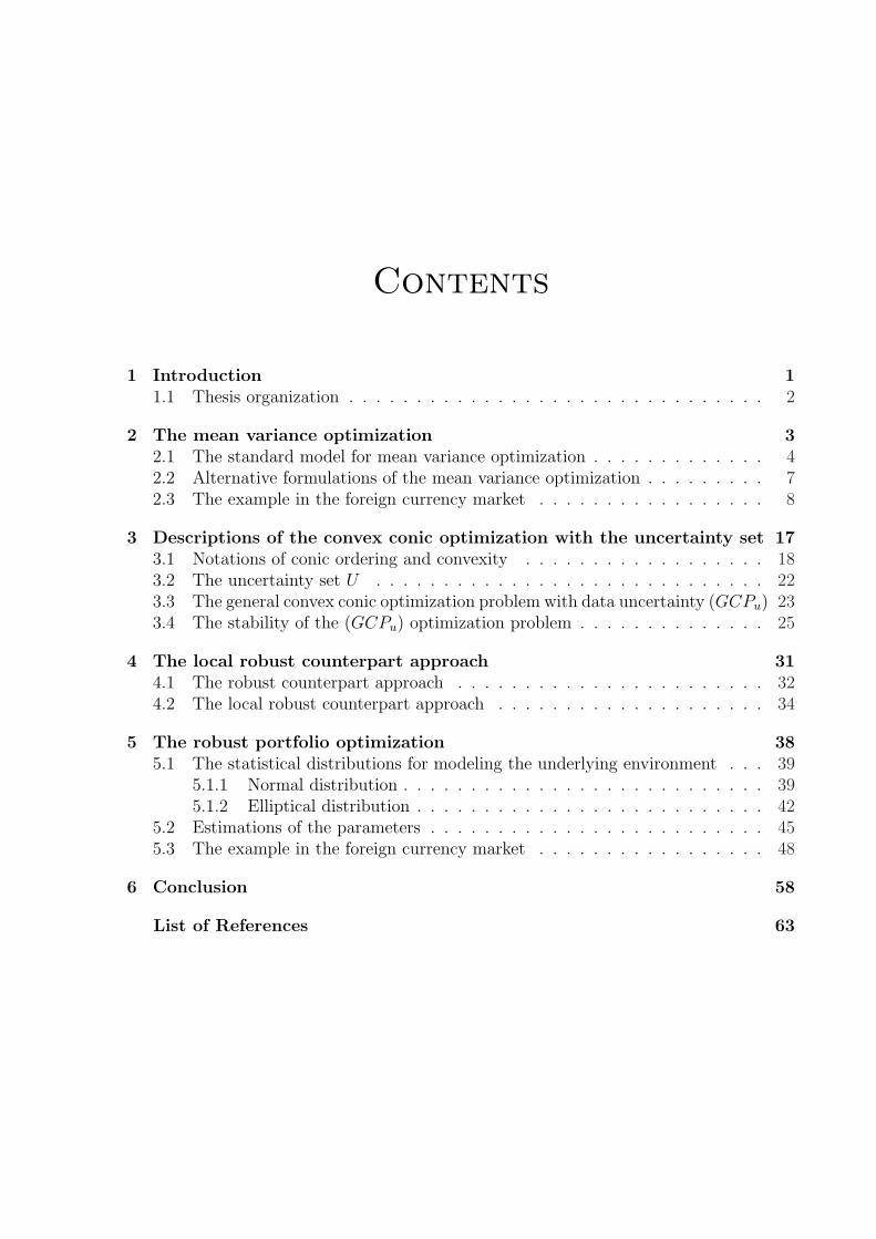
Contents

1 Introduction 11.1 Thesis organization . . . . . . . . . . . . . . . . . . . . . . . . . . . . . . . 2

2 The mean variance optimization 32.1 The standard model for mean variance optimization . . . . . . . . . . . . . 42.2 Alternative formulations of the mean variance optimization . . . . . . . . . 72.3 The example in the foreign currency market . . . . . . . . . . . . . . . . . 8

3 Descriptions of the convex conic optimization with the uncertainty set 173.1 Notations of conic ordering and convexity . . . . . . . . . . . . . . . . . . 183.2 The uncertainty set U . . . . . . . . . . . . . . . . . . . . . . . . . . . . . 223.3 The general convex conic optimization problem with data uncertainty (GCPu) 233.4 The stability of the (GCPu) optimization problem . . . . . . . . . . . . . . 25

4 The local robust counterpart approach 314.1 The robust counterpart approach . . . . . . . . . . . . . . . . . . . . . . . 324.2 The local robust counterpart approach . . . . . . . . . . . . . . . . . . . . 34

5 The robust portfolio optimization 385.1 The statistical distributions for modeling the underlying environment . . . 39

5.1.1 Normal distribution . . . . . . . . . . . . . . . . . . . . . . . . . . . 395.1.2 Elliptical distribution . . . . . . . . . . . . . . . . . . . . . . . . . . 42

5.2 Estimations of the parameters . . . . . . . . . . . . . . . . . . . . . . . . . 455.3 The example in the foreign currency market . . . . . . . . . . . . . . . . . 48

6 Conclusion 58

List of References 63

Notation and Symbols

∅ The empty setd= The equality of the distributions

d(x, y) The distance from a point x to another point ye ∈ Rn The column vector defined as e = (1, · · · , 1)T

H-lsc The abbreviation of Hausdorff lower semicontinuousH-usc The abbreviation of Hausdorff upper semicontinuousinfX The infimum of the set XintX The interior of the set X℘(X) The power set of the set XRn The real n−spaceR+ The nonnegative orthant of R

Vε(x) The ε-neighborhood of a point xVε(X) The ε-neighborhood of a set X

f : Rn → R The objective function from Rn to Rf ∗ : U → R The optimal value functiong : Rn → R The constraint function from Rn to R

E The expected return of the portfolioF The feasible set of the original optimization problemF ∗ The optimal set of the original optimization problemF S The set of Slater points of the original optimization problemFU The set of all feasible solutions for every uncertain parameter u of the original

optimization problemFLRC The feasible set of the local robust counterpart optimization problemF ∗

LRC The optimal set of the local robust counterpart optimization problemF S

LRC The set of Slater points of the local robust counterpart optimization problemµ The expected returns of the assetsρ The correlation

Σ ∈ Rn×n The covariance matrix of the asset returnsσ The standard deviationu The uncertain parameterU The uncertainty setV The variance of the return of portfolio% The risk aversion coefficientx The weights in a portfoliox∗ The optimal solutionX The feasible set

Chapter 1

Introduction

The mean variance optimization problem developed by Markowitz is one of the leading

investment theories in finance. This theory asserts that the return and risk are the

most important two parameters for determining the investment allocation, and on the

basis of the trade-off between the return and risk, the optimal portfolio can be then

obtained. Nevertheless, since the mean variance optimization problem is very sensitive

to the perturbations of the input data, therefore, the optimal portfolio generated by this

optimization problem is not vary reliable if the incorrect parameter values are adopted.

There are various discussions and investigations on how to eliminate or at least decrease

the possibility of using the incorrect input data in the optimization problem. Many papers

propose to use robust estimators as input parameters, some others suggest to reformulate

the optimization problem into the stochastic programming, and a more different approach

to robustification of the optimization problem is to use the idea of resampling which

proposed by Michaud [22] in 1998.

Moreover, Ben-Tal and Nemirovski [3] introduced the other idea of robustification

called the robust counterpart approach by optimizing over an uncertainty set that based

on the incorrect or uncertain data. This specific approach has gained lots interest since it

was established, and many papers were based on the studies of determining the uncertainty

set of the robust counterpart approach.

The main purpose of this dissertation is to study and investigate the robust counterpart

1

approach and then apply this process in the foreign currency market.

1.1 Thesis organization

In Chapter 2, a brief introduction of the basic concept of the Markowitz mean variance

optimization problem will be introduced. In addition, since there are several different but

equivalent formulations of the mean variance optimization problem, therefore, the most

widely used formulations will be presented. The main part of chapter 2 is to show the

fundamental weakness of the mean variance portfolio optimization problem by giving a

simple example in the foreign currency market.

Chapter 3 focuses on the general descriptions of the convex conic optimization problem

with the uncertainty, and the idea of the uncertainty set will be first introduced at this

point. Moreover, the stability statements of the convex conic optimization problem will

be provided as well. The notion of the (local) robust counterpart and the existence of the

Slater point for the robustified optimization problem will be given in chapter 4.

Finally, the robust portfolio optimization by applying the (local) robust counterpart

approach to the general convex conic optimization problem is presented in Chapter 5 with

the example of the foreign currency market. And in order to facilitate the creation of the

ellipsoid uncertainty set for the robust portfolio optimization problem, the concepts of

statistical distributions for modeling the underlying market and parameter estimators for

the inputs will be explained beforehand.

Chapter 2

The mean variance optimization

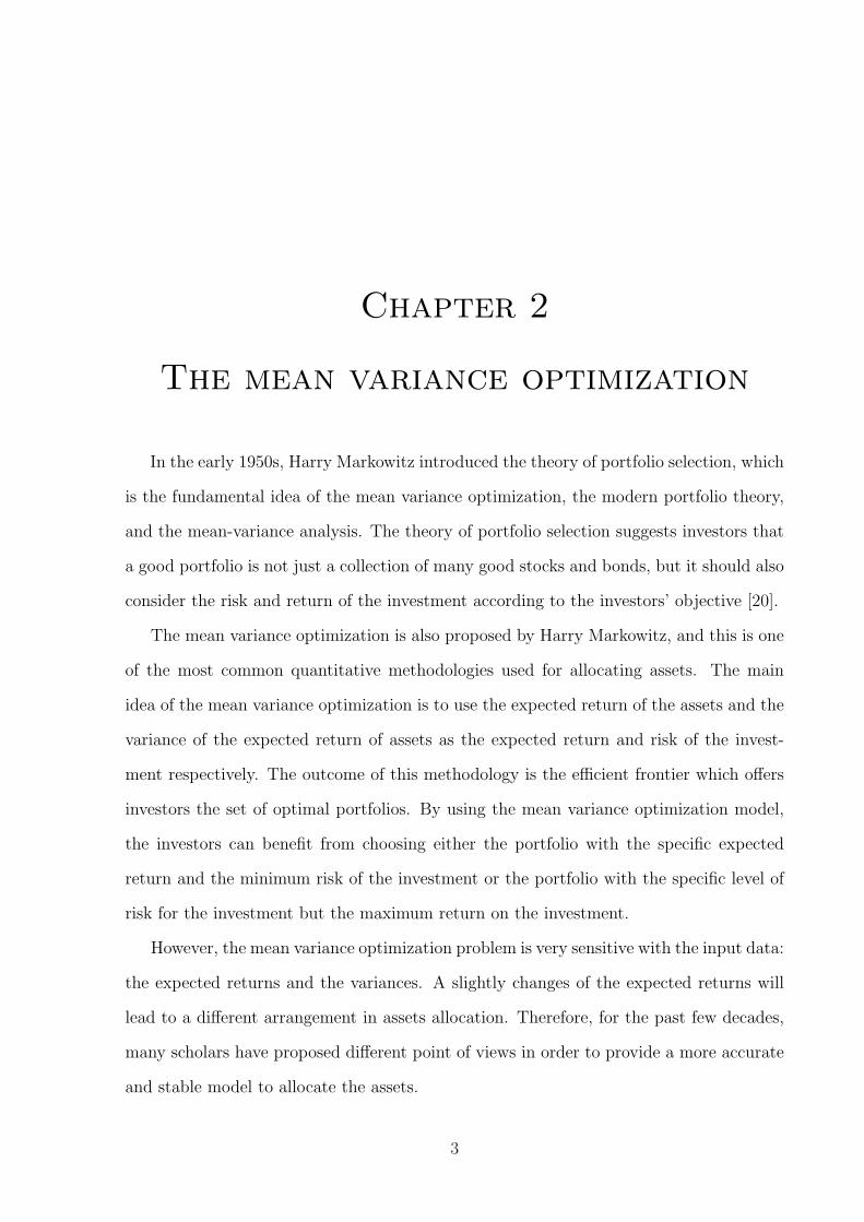
In the early 1950s, Harry Markowitz introduced the theory of portfolio selection, which

is the fundamental idea of the mean variance optimization, the modern portfolio theory,

and the mean-variance analysis. The theory of portfolio selection suggests investors that

a good portfolio is not just a collection of many good stocks and bonds, but it should also

consider the risk and return of the investment according to the investors’ objective [20].

The mean variance optimization is also proposed by Harry Markowitz, and this is one

of the most common quantitative methodologies used for allocating assets. The main

idea of the mean variance optimization is to use the expected return of the assets and the

variance of the expected return of assets as the expected return and risk of the invest-

ment respectively. The outcome of this methodology is the efficient frontier which offers

investors the set of optimal portfolios. By using the mean variance optimization model,

the investors can benefit from choosing either the portfolio with the specific expected

return and the minimum risk of the investment or the portfolio with the specific level of

risk for the investment but the maximum return on the investment.

However, the mean variance optimization problem is very sensitive with the input data:

the expected returns and the variances. A slightly changes of the expected returns will

lead to a different arrangement in assets allocation. Therefore, for the past few decades,

many scholars have proposed different point of views in order to provide a more accurate

and stable model to allocate the assets.

3

This chapter will review the relevant underpinning theories and arguments based on

Cornuejols and Tutuncu [10], Elton, Gruber, Brown and Goetzmann [11], and Markowitz

[21]. Furthermore, it will also address different scholars’ thoughts within the field of

management mathematics in the current literature.

2.1 The standard model for mean variance optimiza-

tion

Before starting the description of the mean variance optimization problem, there are

some assumptions that have to be addressed.

First of all, the markets are perfectly efficient without taxes and transaction costs, and

the investors are assumed to be all risk averse, which means that the investors will only

agree to take higher risk if the higher expected return is offered. In addition, the investors

also prefer higher return than lower and less risk than more. Finally, the model supposes

that the investment decision would only based on the information of the expected returns

and risks.

Consider the model that contains n assets S1, S2, . . . , Sn with weights x1, x2, . . . , xn

invested in those n assets respectively, where

n∑i=1

xi = 1 (2.1)

xi ≥ 0 with i = 1, . . . , n (2.2)

And suppose each individual assets S1, S2, . . . , Sn have expected return µ1, µ2, . . . , µn,

therefore, the expected return of the portfolio E can be stated as:

E =n∑

i=1

xiµi (2.3)

The risk of the investment can be denoted as the variance of the return σ21, σ

22, . . . , σ

2n,

4

and σij as the covariance between asset i and asset j, where

σii = σ2i (2.4)

σij = ρijσiσj (2.5)

and ρij is the correlation between asset i and asset j. Hence, the variance of the return

of portfolio V can be stated as below:

V =n∑

i,j=1

ρijσiσjxixj =n∑

i,j=1

σijxixj (2.6)

By considering the formulas in the form of matrix, the weights of the portfolio w,

the expected returns u, and the covariance between assets Σ = (σij) (a n×n symmetric

matrix with σij = σji and σii = σ2i ) can be written as followed:

x = (x1, . . . , xn)T (2.7)

µ = (µ1, . . . , µn)T (2.8)

Σ = (σij) =

σ11 · · · σ1n

.... . .

...

σn1 · · · σnn

(2.9)

As the result, the expected return of the portfolio E and the variance of return on the

portfolio V can be rearranged as

E = µT x (2.10)

V = xT Σx (2.11)

Definition 2.12 A portfolio in the standard model is feasible if it satisfies the constraint

equations (2.1) and (2.2). In addition, the feasible set is the collection of all feasible

portfolios.

5

Definition 2.13 A feasible portfolio is efficient if it has the maximal expected return

among all other feasible portfolios that have the same level of risk (the same variance),

and has the minimum risk among all other feasible portfolios that have the same expected

return.

Definition 2.14 The efficient frontier is the set of all efficient feasible portfolios.

Definition 2.15 A feasible portfolio is the global minimum variance portfolio (GMV) if

it has the lowest level of risk (the lowest variance).

Figure 2.16 The rough graphical example of the feasible set1

-The Risk V (%)

6

The ExpectedReturn E(%)

u A

uB

u C

u D

u E

uF

In Figure 2.16, the feasible set is the area that bounded by the curve ABC, and all

other portfolios which is outside of the area ABC are the unobtainable portfolios. For

instance, the portfolio D is the portfolio which is not feasible.

The portfolios that belong to the area ABC are all feasible but not all efficient. Except

the portfolios on the arc AB, the rest of the feasible portfolios can be either replaced by

the portfolio with higher expected return but the same level of risk or the portfolio with

the same amount of expected return but less variance. The set of all efficient portfolio

is called the efficient frontier which is the arc AB in Figure 2.16, and the replaceable

portfolios are referred as the inefficient portfolios.

1Figure 2.16 is just a simple sketch that based on Exhibit 2.1 in Fabozzi, Kolm, Pachamanova, andFocardi [12].

6

As shown in the Figure 2.16, both portfolios E and F are feasible, but for taking

the same level of the risk, the portfolio F can offer more amount of return in the fu-

ture. Therefore, the investors will rather choose the portfolio F instead of the inefficient

portfolio E.

Finally, the portfolio B is the feasible portfolio with the lowest level of risk. Therefore,

the portfolio B is the global minimum variance portfolio (GMV).

2.2 Alternative formulations of the mean variance

optimization

There are few alternative formulations of the mean variance optimization problem, and

the most practical three substitutions are the risk minimization formulation, the expected

return maximization formulation and the risk aversion formulation. Those formulations

are different as they have dissimilar investment targets, but on the other hand, they are

equivalent due to the same efficient frontier which is created by using the expected return

and the variance of the portfolio in the similar manner.

The risk minimization formulation is helpful for the investment which requires a mini-

mum variance portfolio with a targeted amount of expected return µ0, and the formulation

is a quadratic optimization problem2 that can be defined as:

minx

xT Σx (2.17)

µT x = µ0

eT x = 1

The expected return maximization formulation is applied when the investment has to

be kept at a specific level of risk. Hence the optimization problem is designed to maximize

2Basically, the quadratic optimization problem is a mathematical optimization that optimizingquadratic function subjects to linear constraints. Please refer to Cornuejols and Tutuncu [10] chapter 7for detailed explanation.

7

the expected return under the restriction of keeping risk at certain level σ20.

maxx

xT µ (2.18)

xT Σx = σ20

eT x = 1

The risk aversion formulation is based on the consideration of the trade-off between the

expected return and the risk of the portfolio by introducing the risk aversion coefficient %.

This coefficient is also named as the Arrow-Pratt risk aversion index and usually settled

between 2 to 4 for the purpose of allocating assets in the investment management.

maxx

(xT µ− %xT Σx) (2.19)

eT x = 1

If the aversion to risk is low, then the coefficient % is small and leads to the results of

more risky portfolios with higher expected return. In the same way, if the risk aversion is

high, then the coefficient % will be large and the optimization problem will result in the

portfolios with less risk and lower expected return.

2.3 The example in the foreign currency market

In the market of the foreign currencies, the exchange rate3 is referred as the price

of the foreign currency in the domestic currency. In other words, the exchange rate is

the price that the investors need to pay in the sterling pounds for one unit of the other

currency, say USD $ 1.

Assuming there is a portfolio with only two foreign currencies, the Euro Se and the

3The exchange rates in this paper are spot rates, unless specified otherwise.

8

US dollar Sus, and the domestic currency is the sterling pound. The time period of the

investment is one month started from 1st of June.

By collecting the historical data from the website of The Bank of England4, the ex-

change rates of the Euro and the US dollar are plotted in the figure below.

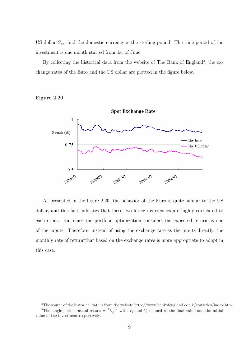
Figure 2.20

As presented in the figure 2.20, the behavior of the Euro is quite similar to the US

dollar, and this fact indicates that these two foreign currencies are highly correlated to

each other. But since the portfolio optimization considers the expected return as one

of the inputs. Therefore, instead of using the exchange rate as the inputs directly, the

monthly rate of return5that based on the exchange rates is more appropriate to adopt in

this case.

4The source of the historical data is from the website http://www.bankofengland.co.uk/statistics/index.htm.5The single-period rate of return = Vf−Vi

Viwith Vf and Vi defined as the final value and the initial

value of the investment respectively.

9

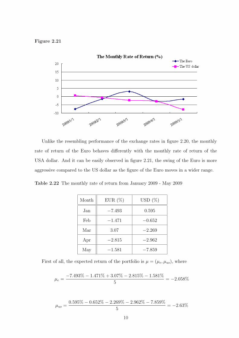
Figure 2.21

Unlike the resembling performance of the exchange rates in figure 2.20, the monthly

rate of return of the Euro behaves differently with the monthly rate of return of the

USA dollar. And it can be easily observed in figure 2.21, the swing of the Euro is more

aggressive compared to the US dollar as the figure of the Euro moves in a wider range.

Table 2.22 The monthly rate of return from January 2009 - May 2009

Month EUR (%) USD (%)

Jan −7.493 0.595

Feb −1.471 −0.652

Mar 3.07 −2.269

Apr −2.815 −2.962

May −1.581 −7.859

First of all, the expected return of the portfolio is µ = (µe, µus), where

µe =−7.493%− 1.471% + 3.07%− 2.815%− 1.581%

5= −2.058%

µus =0.595%− 0.652%− 2.269%− 2.962%− 7.859%

5= −2.63%

10

The variance σ2 = (σ2e , σ

2us) and the covariance Σ between the Euro and the US dollar are

σ2e = 11.397% and σ2

us = 8.379%

Σ =

σ2e σeus

σeus σ2us

=

11.397% −3.351%

−3.351% 8.379%

Therefore, with the weights x = (xe, xus)T , the expected return of the portfolio E and the

variance of the portfolio V are

E = µT x

= −2.058xe%− 2.63xus%

V = xT Σx

=

(xe xus

)

11.397% −3.351%

−3.351% 8.379%

xe

xus

= 11.397x2e% + 8.379x2

us%− 6.702xexus%

Figure 2.23

Figure 2.23 shows the feasible set of the investment in the foreign currencies, and

11

the efficient frontier starts from the global minimum variance portfolio B (44% in Euros

and 56% in US dollars) to portfolio A. Although none of the feasible portfolios provides

possible profit in the future, the maximum expected return portfolio A offers the least

loss by consisting 100% of Euros.

As a matter of the fact, in the single period mean variance optimization problem

as the given foreign currency example here, the maximum expected return portfolio is

always generated by consisting only the asset with the highest expected return. And it

is impossible to make any other portfolio with greater expected return than the highest

expected return asset. But in the case of considering the risk, usually it is possible to

create a less risky portfolio by selecting between different assets, and this is depending on

the covariance between each individual assets.

Furthermore, if using the historical information as the inputs, the more data collected

the more accurate the findings will be. Therefore, instead of using the previous inputs,

the data from January 2000 to December 20086 would be adopted for the comparison

example.

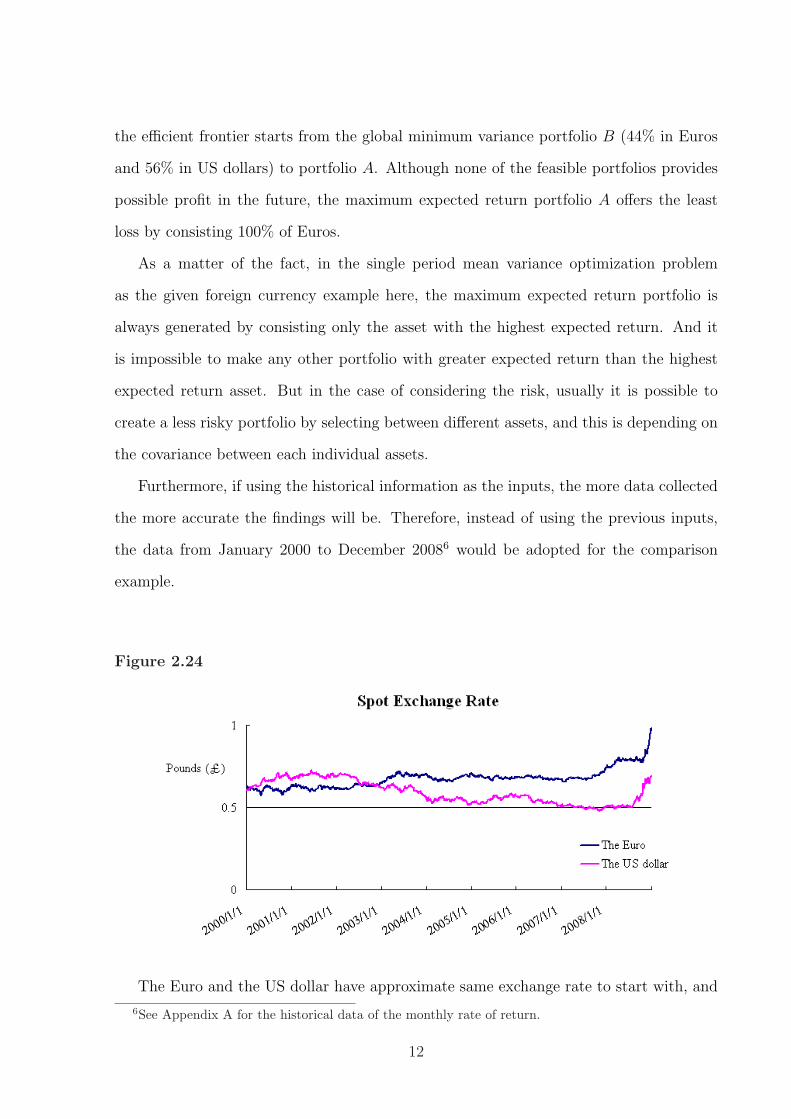
Figure 2.24

The Euro and the US dollar have approximate same exchange rate to start with, and

6See Appendix A for the historical data of the monthly rate of return.

12

the US dollar was stronger than the Euro in the first two years but then started to decline

till year 2008. On the contrary, the value of the Euro increases 53% over the past nine

years. Figure 2.24 furthermore shows the currencies have opposite performances from year

2000 to year 2003, but since then, the behavior of the currencies become more positive

correlated.

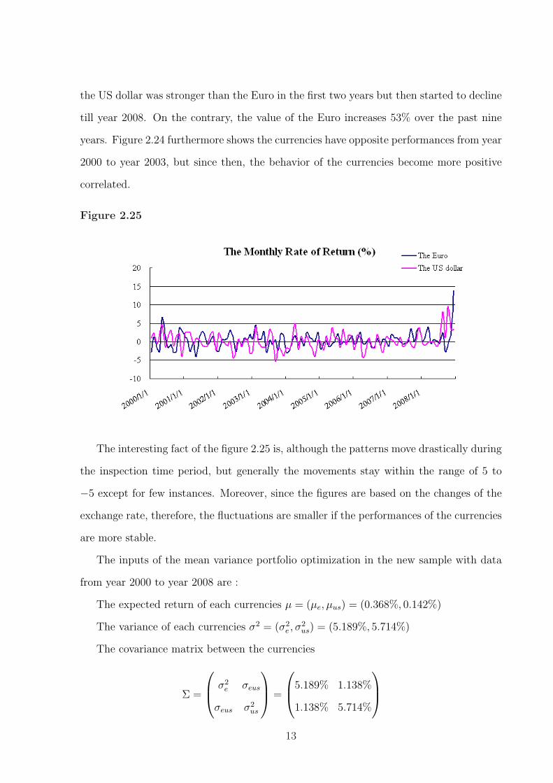
Figure 2.25

The interesting fact of the figure 2.25 is, although the patterns move drastically during

the inspection time period, but generally the movements stay within the range of 5 to

−5 except for few instances. Moreover, since the figures are based on the changes of the

exchange rate, therefore, the fluctuations are smaller if the performances of the currencies

are more stable.

The inputs of the mean variance portfolio optimization in the new sample with data

from year 2000 to year 2008 are :

The expected return of each currencies µ = (µe, µus) = (0.368%, 0.142%)

The variance of each currencies σ2 = (σ2e , σ

2us) = (5.189%, 5.714%)

The covariance matrix between the currencies

Σ =

σ2e σeus

σeus σ2us

=

5.189% 1.138%

1.138% 5.714%

13

With the weights of the portfolio x = (xe, xus)T , the expected return of the portfolio E

and the variance of the portfolio V can be estimated as below.

E = µT x

= 0.368xe% + 0.142xus%

V = xT Σx

=

(xe xus

)

5.189% 1.138%

1.138% 5.714%

xe

xus

= 5.189x2e% + 5.714x2

us% + 2.276xexus%

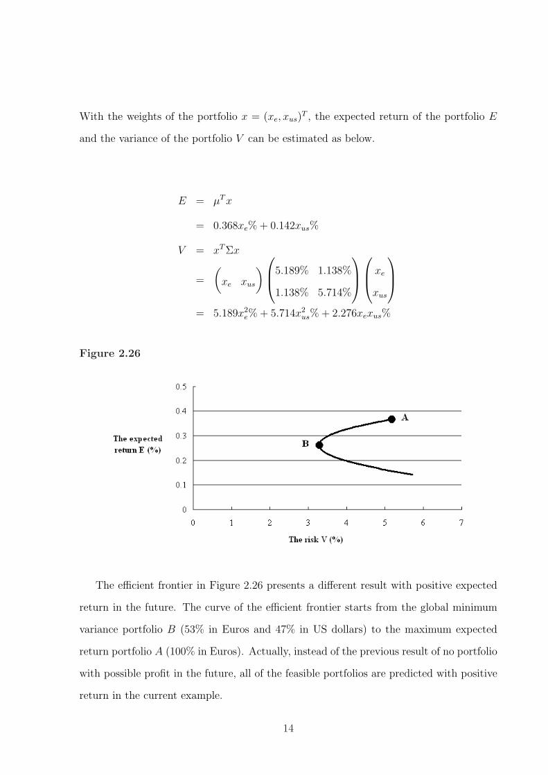
Figure 2.26

The efficient frontier in Figure 2.26 presents a different result with positive expected

return in the future. The curve of the efficient frontier starts from the global minimum

variance portfolio B (53% in Euros and 47% in US dollars) to the maximum expected

return portfolio A (100% in Euros). Actually, instead of the previous result of no portfolio

with possible profit in the future, all of the feasible portfolios are predicted with positive

return in the current example.

14

Judging from the above, the inputs of the mean variance portfolio optimization are very

important in this methodology. The different sampling data will effect the final investment

decision. For instance, if the investor uses the information as the first example, he/she

might decide not invest anything at the present and prefer to wait and observe the market

movement. But the second example says a different story, and the investor may have the

chance to gain some profit.

According to Best and Grauer [5], the changes in the expected return of assets have a

great effect on the estimation of efficient portfolios, and this kind of argument has been well

studied by several scholars. Frankfurter, Phillips and Seagle [14] used the experimental

results to show that the portfolio which selected by the mean variance optimization is

unlikely to be as efficient as the equally weighted portfolio, and Britten-Jones [8] showed

that the estimations of efficient portfolio weights are extremely sensitive to the estimation

errors in the expected return and covariances of the assets.

Instead of concerning the effects of the estimation errors in the expected return, there

are some discussions based on the influence of the covariances between assets. Laloux,

Cizeau, Bouchaud and Potters [19] have discovered that the mean variance optimization

only uses the historical information to determinate the correlation matrix, and the eigen-

values which suppose to control the smallest risk portfolio is dominated by noise. Pafka

and Kondor [25] agree with the above finding, and propose to add some constrains on the

correlation matrix in order to remove the unnecessary factors and capture the essence of

the real correlation structure.

However, some other scholars have suggested another method to solve the issue of the

estimation errors, and the main idea of this methodology is to use a set of scenarios instead

of a fixed value for a particular parameter. Mulvey, Vanderbei and Zenios [24] used an

approach based on the idea of the stochastic programming to generate the solutions from

the set of scenarios, and controlled the stability of the solutions by applying the penalty

functions. On the other hand, Ben-Tal and Nemirovski [3] considered the uncertain data

as the uncertainty set and established the so-called robust counterpart approach to solve

15

the problem with the uncertainty set.

In the later chapters of this paper, the more detailed notion of optimizing with uncer-

tainty will be presented.

Chapter 3

Descriptions of the convex conic

optimization with the uncertainty

set

The character of a mathematical optimization problem is either minimizing or max-

imizing an objective function f : Rn −→ R in a feasible set X ∈ Rn, and usually the

feasible set X is restricted by certain constraint functions gi : Rn −→ R, i = 1, . . . , m.

Generally, the optimization problem can be formulated in the form:

minx

f(x) (3.1)

subject to gi(x) ≤ bi i = 1, 2, . . . , m

with the optimization variable, a vector x = (x1, x2, . . . , xn) in Rn, and the limits of the

constraint function, constants b1, b2, . . . , bm. The outcome of the optimization problem

(3.1) is a vector x∗ ∈ Rn named the optimal solution, and except it has satisfied the

constrain functions gi, it also has the smallest value among all other possible vectors, that

is : f(x∗) ≤ f(y) for any vector y ∈ Rn that satisfies g1(y) ≤ b1, . . . , gm(y) ≤ bm.

There are many different categories of the optimization problems, depending on par-

ticular forms of the objective and constraint functions. For instance, the optimization

problem (3.1) is a convex optimization problem if the objective function and the con-

17

straint functions are convex. i.e., ∀x, y ∈ Rn and α ∈ R with 0 6 α 6 1

f(αx + (1− α)y) ≤ αf(x) + (1− α)f(y) (3.2)

gi(αx + (1− α)y) ≤ αgi(x) + (1− α)gi(y) for i = 1, . . . , n

This chapter is emphasis on presenting the convex conic optimization and the corre-

sponding stability of the optimization problem addressed from [26]. And basically, the

convex conic optimization is one type of the mathematical optimization problem that

searches the optimal solution of a convex real-valued function defined on a convex cone.

To begin with, some basic definitions and properties of the convex cone will be

extracted from the following books : Boyd and Vandenberghe [6] and Brinkhuis and

Tikhomirov [7].

3.1 Notations of conic ordering and convexity

Let K ⊂ Rn be a nonempty set.

• The set K is convex if : ∀x, y ∈ K, 0 ≤ α ≤ 1 ⇒ αx + (1− α)y ∈ K.

• The set K is a cone if : ∀x ∈ K and ∀λ ∈ R with λ ≥ 0 ⇒ λx ∈ K.

• The set K is a convex cone if K is a cone and is also convex1.

• The cone K is pointed if K ∩ (−K) = {0K}.2

• The cone K is solid if K has nonempty interior3,and the interior of the cone K is

denoted by intK.

• The cone K is an ordering cone (also named the proper cone) if it is closed, convex,

pointed, and solid.

1A cone K is convex if and only if x + y ∈ K ∀x, y ∈ K2The zero element of the cone K is called the vertex 0K .3A point (k) is the interior point of K if ∃ε > 0, such that Vε(k) = {x ∈ Rn| ‖x− k‖ ≤ ε} ⊂ K.

18

Definition 3.3 For each ordering cone K ⊂ Rn and x, y ∈ Rn, the cone ordering ºK on

Rn can be defined by x ºK y ⇐⇒ x − y ∈ K. In addition, x ÂK y ⇐⇒ x − y ∈ intK

defined the strict cone ordering.

Proposition 3.4 Let K ⊂ Rn be a nonempty proper cone and ºK be the order relation

imposed by K in Rn. Then the following conditions are satisfied for any arbitrary w,x,y,z∈Rn.

• Reflexivity : x ºK x.

• Transitivity : x ºk y and y ºK z ⇒ x ºK z.

• Compatibility : x ºK y and ∀λ ∈ R with λ ≥ 0 ⇒ λx ºK λy.

• Compatibility : x ºK y and w ºK z ⇒ x + w ºK y + z.

• Antisymmetry : x ºK y and x ¹K y ⇒ x = y.

Definition 3.5 Let K ⊂ Rn be a proper cone with cone ordering ¹K, then f : Rm → Rn

is K-convex if ∀x, y ∈ Rm and 1 ≥ α ≥ 0

f(αx + (1− α)y) ¹K αf(x) + (1− α)f(y). (3.6)

The function f is called strictly K-convex if ∀x, y ∈ Rm, x 6= y, and 1 > α > 0

f(αx + (1− α)y) ≺K αf(x) + (1− α)f(y). (3.7)

Definition 3.8 Let K ⊂ Rn be a cone, the dual cone of the cone K is the set

K∗ = {y ∈ Rn | xT y ≥ 0 ∀x ∈ K} (3.9)

The dual cone K∗ of the cone K is a closed convex cone, and has several characteristic

properties. For instance, if K has nonempty interior, then K∗ is pointed; and if the

19

closure of K is pointed, then K∗ has nonempty interior; furthermore, K∗∗ is the closure

of the convex hull of K, and the last feature implies that if K is a closed convex cone,

then K∗∗ = K. In addition, a cone is said to be self-dual if K = K∗.

Example 3.10 One of the simple examples to illustrate cone ordering and the dual cone

is the set K of nonnegative numbers in R, i.e., K = R+. Although the set K is only a

group of positive numbers on the real line, it still qualifies as a proper cone with the cone

ordering ¹K performs as the inequality ≤. And the dual cone K∗ of cone K is

K∗ = {y ∈ R | yT x ≥ 0 ∀x ∈ K}

= {y ∈ R | yT x ≥ 0 ∀x ∈ R+}

= {y ∈ R | y ≥ 0}

= R+

= K

This example can be extend to the case when the set K is the first orthant in Rn,

K = Rn+ = {x ∈ Rn | xi ≥ 0 i = 1, 2, . . . , n}, then K is a proper cone with the

coordinatewise order between vectors, i.e.,

x ≥ y ∀x, y ∈ Rn ⇔ xi ≥ yi ∀i = 1, . . . , n.

The dual cone K∗ of cone K = Rn+ is given by

K∗ = {y ∈ Rn | yT x ≥ 0 ∀x ∈ K}

= {y ∈ Rn | yT x ≥ 0 ∀x ∈ Rn+}

= {y ∈ Rn | yi ≥ 0 i = 1, 2, . . . , n}

= Rn+

= K

20

Proposition 3.11 Let K ⊂ Rn be a proper cone with cone ordering ¹K, then the function

f : Rm → Rn is K-convex if and only if zT f(.) is convex ∀z ºK∗ 0.

Proof. If the function f is K-convex, then ∀x, y ∈ Rm and α ∈ [0, 1]

f(αx + (1− α)y) ¹K αf(x) + (1− α)f(y) (3.12)

By Definition 3.3, (3.12) is equivalent to

αf(x) + (1− α)f(y)− f(αx + (1− α)y) ∈ K (3.13)

By Definition 3.8,

∀z ∈ K∗ (αf(x) + (1− α)f(y)− f(αx + (1− α)y))T z ≥ 0

⇒ 〈αf(x) + (1− α)f(y)− f(αx + (1− α)y), z〉 ≥ 0

⇒ 〈z, αf(x)〉+ 〈z, (1− α)f(y)〉 − 〈z, f(αx + (1− α)y)〉 ≥ 0

⇒ α〈z, f(x)〉+ (1− α)〈z, f(y)〉 ≥ 〈z, f(αx + (1− α)y)〉

⇒ αzT f(x) + (1− α)zT f(y) ≥ zT f(αx + (1− α)y)

Therefore, zT f is convex ∀z ∈ K∗.

The converse proof also follows directly from the same definitions; hence it would be

omitted. ¤

Moreover, if the cone K ⊂ Rn has nonempty interior, then

x ∈ intK ⇔ yT x > 0 ∀ y ∈ K∗\{0}. (3.14)

21

3.2 The uncertainty set U

One of the serious concerns in most of the optimization problems is the accuracy of

the input data. Sometimes this matter can be as simple as the inputs are unknown at

the time the optimization problem must be solved; sometimes the inputs are incorrectly

computed or just uncertain. As mentioned in Chapter 2, the result of the optimization

problem is very sensitive to those input data. And with different inputs, the optimization

problem will lead us to the solution that is far from the optimal of the original problem.

The uncertainty of the inputs can be simply modeled by introducing an uncertainty

set U that contains many possible values of required uncertain parameters. And there

is a corresponding constraint for each uncertain parameter u ∈ U to ensure the original

optimization constraint is fulfilled for the worst-case of the uncertainty set U .

In general, the shape of the uncertainty set U depends on the sources of uncertainty and

also the sensitive affection of the uncertainty. The most common shapes of the uncertainty

set are interval, ellipsoid and the intersection of the ellipsoids. Schottle [26] investigated

the effects of interval and ellipsoidal uncertainty set on the continuity properties of the

optimal solution set. The result illustrated that under certain conditions, the ellipsoidal

uncertainty set smoothen the optimal value function, and in most practical cases the

ellipsoidal uncertainty set lead to a unique optimal solution that is continuous with respect

to the uncertain parameter.

The size of the uncertainty set U depends on the desired robust level of the optimiza-

tion problem. Some scholars mentioned that the price for the optimization problem with

uncertainty set to be stable can be measured in the term of the increase of the optimal

value from the original one, and the amount that rose in the optimal value is linear in the

size of the uncertainty set. Ben-Tal and Nemirovski [3] used the linear problems to prove

the above statement, and Schottle [26] obtained the same result by examine the convex

conic problems.

In addition, Calafiore and Campi [9] proposed to use the scenario approach that based

22

on the constraint sampling to deal the uncertainty of the optimization problem. The

uncertainty set of this methodology is defined as a collection of scenarios for the uncertain

parameters, and there is one constraint for each scenario. Therefore, the outcome of the

modified optimization problem needs to be qualified for all the constraints that generated

by the corresponding scenario. And the number of the required scenarios for the portfolio

with n assets can be calculated by fixing the desired level parameter4 ε ∈ [0, 1] and

confidence parameter β ∈ [0, 1]:

The number of the scenarios ≥ n

εβ− 1

3.3 The general convex conic optimization problem

with data uncertainty (GCPu)

This section presents the setting for the convex conic optimization problem that de-

pends on the particular uncertain parameter. And for easy reference, some notations and

assumptions that will be used throughout the article will be introduced beforehand:

• u, the vector that represent the uncertain parameter.

• x, the vector that represent the decision parameter.

• U ⊂ Rd, the nonempty convex and compact set of the uncertain parameters.

• X ⊂ Rn, the nonempty convex and compact set of decisions that do not depend on

the uncertain parameter u.

• K ⊂ Rm, the ordering cone, i.e., K is closed, solid, convex and pointed.

• f : Rn × Rd → R, the objective function that is continuous in x and u, and f is

convex in u for fixed x ∈ X, and convex in x for fixed u ∈ U .

4The accepted possibility that the original constraint may violated throughout the process of theoptimization

23

• g : Rn × Rd → Rm, the constraint function that is continuous in x and u, and g is

K−convex in u for fixed x ∈ X, and K−convex in x for fixed u ∈ U .

Definition 3.16 The general convex conic optimization that based on the uncertain pa-

rameter u, (GCPu), can be formulated as

minx∈X

f(x, u) (3.17)

subject to g(x, u) ¹K 0

Definition 3.18 For a given u ∈ U in the general convex conic optimization problem,

the feasible set, the optimal set, and the set of Slater points can be stated as :

• The feasible set F (u) : {x ∈ X | g(x, u) ¹K 0}.

• The optimal set F ∗(u) : {x ∈ F (u) | f(x, u) ≤ f ∗(u)}.

• The set of Slater points F S(u) : {x ∈ X | g(x, u) ≺K 0}.

where f ∗ : U → R is the optimal value function defined as

f ∗(u) := min{f(x, u) | x ∈ F (u)}, (3.19)

and the set of all feasible solutions for every u ∈ U is FU =⋂

u∈U

F (u).

Additionally, for each u ∈ U in the general convex conic optimization, the functions

that assign the feasible set F (u) and the optimal set F ∗(u) are

• The feasible set mapping F : U →℘(X).

• The optimal set mapping F ∗ : U →℘(X).

where ℘(X) is the power set of the set X.

Finally, throughout this paper, the set of the solutions that are feasible for all u ∈ U

is assumed to be nonempty unless in the particular situation.

24

Assumption 3.20 There is at least one feasible solution x ∈ X for all parameters within

the uncertainty set U , FU 6= ∅ ∀u ∈ U .

3.4 The stability of the (GCPu) optimization problem

In the previous sections, we were only concerned about the setting of the (GCPu)

optimization problem without paying any attention to the corresponding stability of the

optimization problem. Generally speaking, a solution of the optimization problem is stable

if the solution is not effected too much by the small perturbations of the input data. And

the stability property of the optimization problem can be expressed as the continuous

mapping5 between the input data and the solutions of the optimization problem.

Definition 3.21 A mapping h : X → Y is continuous for some x ∈ X if for any

neighborhood V of h(x) there is a neighborhood U of x such that h(U) ⊂ V .

One of the important requirements for examining the stability (continuity) of the

optimization problem is the existence of at least one solution for the optimization problem,

and this requirement can be assured by the Assumption 3.20, FU 6= ∅, together with the

objective function f being continuous. Consequently, the optimal solution set F ∗(u) of

the (GCPu) optimization problem is nonempty for every u ∈ U .

Schottle [26] derived the stability of the (GCPu) optimization problem by applying

the concepts of the Hausdorff continuity and the Berge continuity. In addition, Schottle

proposed that with respect to the parameter u ∈ U , the appearance of the Slater point

guarantees the Hausdorff upper semi-continuous property of the feasible set mapping F

even under the situation of more than one solution. And the Slater point can be obtained

if the constraint function g(·, u) of the (GCPu) optimization problem is strictly K−convex.

That is, suppose x, y ∈ F (u) are any two solutions of u ∈ U , and since F (u) is a convex

5The ideas of the continuous mapping (function) are:

• For a function f(.), the value of f(x) , where x is a certain point belongs to the domain of f(.),can be predicted by using the value of f(.) at some points near x.

• The graph of the function f(.) is a connected curve without any jumps, holes and gaps.

25

set, then for all α ∈ [0, 1] a point z := αx + (1 − α)y also belongs to the set F (u), such

that

g(z, u) = g(αx + (1− α)y, u). (3.22)

If the constraint function g(·, u) is strictly K−convex as required, then the point z :=

αx + (1− α)y satisfies the following equation

g(αx + (1− α)y, u) ≺K αg(x, u) + (1− α)g(y, u), (3.23)

and by the definition of the feasible set, g(x, u) ¹K 0 and g(y, u) ¹K 0. Hence, equation

(3.23) becomes

g(αx + (1− α)y, u) ≺K 0 (3.24)

which is equivalent to

g(z, u) ≺K 0. (3.25)

As the result, the point z ∈ F (u) is a Slater point of the (GCPu) optimization problem.

Before continuing the investigation about the stability of the (GCPu) optimization

problem, there are some necessary definitions that extracted from the book by Bank [2]

need to be addressed.

Definition 3.26 The ε−neighborhood of a set S ⊂ Rn with ε > 0 is defined by

Vε(S) := {x ∈ Rn | d(x, S) = infy∈S

d(x, y) < ε}. (3.27)

Definition 3.28 A point−to−set mapping Γ : U → ℘(Rn) is closed at a point u if the

26

sequences

uk → u, {uk} ⊂ U

with xk ∈ Γ (uk), k = 1, 2, . . . , imply x ∈ Γ (u),

xk → x, {xk} ⊂ Rn

and the mapping Γ is closed if it is closed at every point of U .

Definition 3.29 The mapping Γ is Hausdorff upper semi-continuous at the point u if

for each ε > 0 there is δ > 0, such that

Γ (u) ⊂ Vε(Γ (u)) ∀u ∈ Vδ(u), (3.30)

and the mapping Γ is Hausdorff lower semi-continuous at the point u if for each ε > 0

there is δ > 0, then

Γ (u) ⊂ Vε(Γ (u)) ∀u ∈ Vδ(u). (3.31)

Definition 3.32 The mapping Γ : U → ℘(Rn) is Hausdorff continuous at the point u if

Γ is Hausdorff upper semi-continuous and also Hausdorff lower semi-continuous at the

point u.

Remark 3.33 The mapping Γ : U → ℘(Rn) is Hausdorff upper semi-continuous at

u ∈ U if Γ is closed and the set X is compact.

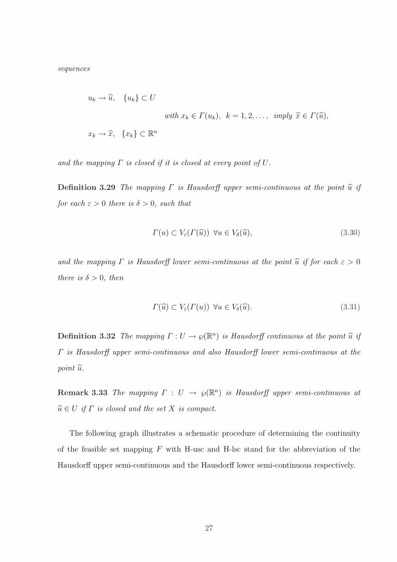
The following graph illustrates a schematic procedure of determining the continuity

of the feasible set mapping F with H-usc and H-lsc stand for the abbreviation of the

Hausdorff upper semi-continuous and the Hausdorff lower semi-continuous respectively.

27

Figure 3.34

minx f(x, u)subject to g(x, u) ¹K 0

?g is continuous and the cone K is closed

The mapping F is closed

?The decision set X is compact

The mapping F is H-usc

QQ

QQ

QQ

QQ

QQ

QQQs

∃ unique solution

The mapping F is H-lsc

?

∃ More than one solutionand g ≺K 0

´´

´´

´´

´´

´´

´´+

∃ Slater points

?

The mapping F is H-lsc

?

The mapping F is Hausdorff continuous at u

First of all, the feasible set mapping F is closed under the assumptions of the constraint

function g is continuous and the cone K is closed. Consequently, the closedness of the

mapping F together with the set X being compact verify that the mapping F is Hausdorff

upper semi-continuous for all u ∈ U .

28

Now, according to the assumption FU 6= ∅ for all u ∈ U , there is either a unique

solution or more than one solutions for each u ∈ U . Hence, instead of describing the

Hausdorff lower semi-continuity of the mapping F as one single case, the following two

situations will be considered.

• The solution is unique for each u ∈ U .

• There exists more than one solution for each u ∈ U .

In the case of only one solution for each u ∈ U , the Hausdorff upper semi-continuity

of the feasible set mapping F : U →℘(X) imply the following :

Let u ∈ U , for ε > 0 there exists δ > 0, such that

F (u) ⊂ Vε(F (u)) ∀u ∈ Vδ(u). (3.35)

And because F (u) is the only solution for u, therefore F (u) ∈ Vε(F (u)), where

Vε(F (u)) = {y ∈ Rn | d(y, F (u)) < ε}. (3.36)

Since F (u) ∈ Vε(F (u)), then it implies

d(z, F (u)) < ε ∀z ∈ F (u), (3.37)

and hence

F (u) ∈ Vε(z) ∀z ∈ F (u). (3.38)

Which is equivalent to

F (u) ∈ Vε(F (u)). (3.39)

29

Therefore, the feasible set mapping F is Hausdorff lower semi-continuous for all u ∈ U in

this case.

Under the circumstance of more than one solution for u ∈ U , the Slater point exists

if the constraint function g(·, u) is strictly K−convex. And according to [26], the feasible

set mapping F is Hausdorff upper semi-continuous at u ∈ U if there is a Slater point of

F (u).

Eventually, with both Hausdorff upper semi-continuity and Hausdorff lower semi-

continuity at u, the feasible set mapping F is Hausdorff continuous at u.

Chapter 4

The local robust counterpart

approach

In 1998, Ben-Tal and Nemirovski published their paper [3] on deriving the robust coun-

terpart approach for the optimization problem with uncertain parameters. This robust

counterpart approach is in fact the worst-case approach of the original optimization prob-

lem, as the modified optimization problem is not only solved the problem for every point

of the uncertain set, but is concerned specially the case with the worst performance. On

the ground of this development, Ben-Tal and Nemirovski have continuously investigated

the robust counterpart approach in various situations, and one of their recent journals [4]

summarized several selected topics of the robust counterpart, especially on the concept

of the extended idea and the tractability of the robust counterparts.

Before the introduction of the robust counterpart approach, there are several method-

ologies to deal with the uncertainty. The most common techniques are the sensitivity

analysis and the stochastic programming. In many optimization problems, the uncertain

data are replaced by the nominal values and then justified the stability of the results by

the sensitivity analysis which only deals with the trivial deviations of the nominal data.

On the other hand, the stochastic programming pays attention to the uncertain data from

the beginning of the problem, but this method has the following weaknesses: the solution

may not satisfy the required constraint and the price of using the stochastic programming

31

to solve the problem can be very expensive.

Apart from those already mentioned techniques, another approach to solve the opti-

mization problem with uncertainty is the robust mathematical programming developed

by Mulvey, Vanderbei and Zenios in 1995 [24]. This programming uses a set of scenarios

instead of the fixed nominal data (point estimates), but has the same disadvantage as

the stochastic programming. The robust mathematical programming might leads to the

solutions that unfulfilled the constraint.

The main motivation of this chapter is to present the local robust counterpart approach

together with the stability of the local robust counterpart problem proposed by Schottle

[26]. And to begin with, the concept of the robust counterpart approach by Ben-Tal and

Nemirovski [3] would be discussed first.

4.1 The robust counterpart approach

As already mentioned, the robust counterpart approach is the worse -case approach of

the original optimization problem with the uncertainty. This methodology first assumes

the uncertain parameters may vary in a particular set, and then find the portfolio weights

to optimize the objective function even if the ”worse” case turns out in the reality.

If the uncertainty set is finite, i.e., U = {u1, u2, . . . , un}, then the optimization problem

can be solved by transferring the function that contains the uncertain parameter into

finitely many functions for every single u ∈ U , and similar process can be applied if there

are finitely many vertices belong to the uncertainty set U . Since the transferring process

is only duplicated the particular function, therefore, the original optimization problem is

turned into a larger version but not more difficult due to the structural properties of the

original optimization problem are preserved. For instance, consider the following general

optimization problem with the uncertainty u:

minx

f(x, u) (4.1)

subject to g(x, u) ∈ K

32

If the uncertainty set is a finite set U = {u1, u2, . . . , un}, then the robust counterpart of

the general optimization problem (4.1) can be formulated as :

minx,z

z (4.2)

subject to z − f(x, ui) > 0 i = 1, 2, . . . , n

g(x, ui) ∈ K i = 1, 2, . . . , n

On the other hand, if the uncertainty set is not finite, i.e., continuous set in the shape

of intervals, ellipsoids or the intersections of ellipsoids, then the optimization problem

would be modified into a more complicated process as the function that contains the

uncertain parameter has to be satisfied for all values in the uncertainty set, and there

would be infinitely many constraints needed to be fulfilled in order to solve the function

with the uncertain parameter. Hence this converts the original optimization problem into

the semi-infinite optimization problem.

The robust counterpart of the (GCPu) optimization problem, the general convex conic

optimization problem with uncertain data u, is a semi-infinite programming, which takes

care the problem of the appearance of the worse value of the uncertainty without changing

the original features of the (GCPu) problem, and is formulated as:

minx

maxu

f(x, u) (4.3)

subject to g(x, u) ¹K 0 ∀u ∈ U

where x ∈ X and u ∈ U . And according to the assumption FU 6= ∅ of the (GCPu)

optimization problem, there is a nonempty feasible set for every single u ∈ U . This

implies that the robust counterpart optimization problem also has the nonempty feasible

set, and hence (4.3) is equivalent to:

minx∈FU

maxu∈U

f(x, u) (4.4)

33

4.2 The local robust counterpart approach

This section describes the local robust counterpart approach which based on the

robust counterpart approach that mentioned in the previous section. Compared with the

robust counterpart approach, the local robust counterpart approach concerns only the

smaller area around a particular parameter u of the uncertainty set instead of the entire

uncertainty set U , and hence not all of the values in the uncertainty set U require to fulfill

the constraint of the local robust counterpart problem.

Definition 4.5 The local uncertainty set Uδ(u) ⊂ U centered at u with a suitable ratio

of size δ > 0 is defined as:

Uδ(u) = (u + δU) ∩ U

For example, the original uncertainty set U centered at the point u0 can be displayed

in the same format with δ = 1:

U = Uδ(u0) = (u0 + δU) ∩ U = U.

Definition 4.6 For any u ∈ U and δ > 0, the pair (u, δ) is called acceptable if the

corresponding set u + δU is a subset of the original uncertainty set U .

In some occasions, the shape of the local uncertainty set Uδ(u) is not elliptical as

expected, i.e., some values of Uδ(u) is not within the uncertainty set U . The following

figures illustrate 3 examples of the local uncertainty set Uδ(u).

34

Figure 4.7 The original uncertainty set U

Figure 4.8 The local uncertainty set Uδ(u) with unacceptable pair (u, δ)

Figure 4.9 The local uncertainty set Uδ(u) with acceptable pair (u, δ)

35

Definition 4.10 The local robust counterpart problem (LRCu,δ) of the (GCPu) optimiza-

tion problem with u ∈ U and δ > 0 be the acceptable pair is formulated as:

minx

maxu

f(x, u) (4.11)

subject to g(x, u) ¹K 0 ∀u ∈ Uδ(u)

where x ∈ X and u ∈ Uδ(u).

And under assumption 3.20 (FU 6= ∅), the feasible set of the local robust counterpart

problem is also nonempty, hence the formulation of the (LRCu,δ) problem can be stated

in the same way as equation (4.4).

minx∈FUδ(u)

maxu∈Uδ(u)

f(x, u) (4.12)

The related notations and formulations for the local robust counterpart optimization

problem (LRCu,δ) would be stated in the Appendix B.

In view of the fact that the existence of a Slater point is an important factor for the

stability of the (GCPu) optimization problem. Therefore, the notion of the Slater point

for the local robust counterpart problem will be discussed to close this chapter.

By definition, a point x ∈ X is a Slater point of the (LRCu,δ) problem if

g(x, u) ≺K 0 ∀u ∈ Uδ(u) (4.13)

or equivalently,

g(x, u) ∈ int(−K) ∀u ∈ Uδ(u) (4.14)

And if x ∈ X is a Slater point of the (LRCu,δ) problem, then there exists ε > 0 such that

Vε(g(x, u)) ⊂ int(−K) ∀u ∈ Uδ(u) (4.15)

36

Schottle [26] has proposed that the existence of the Slater point of the the (GCPu)

optimization problem implies the existence of the Slater point of the (LRCu,δ) problem.

And in addition, there is a global ratio of size δglob > 0 such that the (LRCu,δglob)

problem holds a Slater point for any u ∈ intU if the constraint function g is globally

Lipschitz continuous1 for all u ∈ U .

1A mapping f : X → Y is Lipschitz continuous on a set S ⊂ X if for some constant L > 0 and∀s1, s2 ∈ S the following holds ‖ f(s1)− f(s2) ‖6 L ‖ s1 − s2 ‖ .

Chapter 5

The robust portfolio optimization

The mean variance optimization introduced by Markowitz is also refereed as the portfo-

lio optimization that allows the investors to choose the portfolio with the highest expected

return for a given level of risk. This methodology of allocating the assets is famous and

widely used in the field of investment. However, as showed in the chapter 2, the out-

come of the mean variance optimization is extremely sensitive to the perturbations in the

inputs, and hence the subsequent solutions are not very reliable.

There are many discussions on how to decrease or eliminate the possibility of using

incorrect inputs for the optimization problem. Some suggest to use the parameter estima-

tors as inputs in order to reduce the sensitivity of the optimal portfolio, and on the other

hand, Michaud [22] proposed to use the technique of resampling the input parameters

from a confidence region and then average the cumulative portfolios that obtained by

each pair of sampling data. The main idea here is, if resampling enough times, then the

averaged optimal portfolio should be more stable and less sensitive to the perturbations

in the inputs. But this methodology is not efficient when the amount of assets becomes

large.

This chapter presents the application of the local robust counterpart approach for the

mean variance portfolio optimization problem in the foreign currency market, and this

procedure suppose to provide more stable optimal portfolios even under the situation

with the uncertain inputs. In the framework of this modified optimization problem, the

38

uncertain or incorrect parameters are simply modeled by a bounded uncertainty set U ,

but there is no specific definition or restriction for the uncertainty set U in the modified

optimization problem.

In order to define the uncertainty set for the portfolio optimization, one can first as-

sumed the input data follows a multivariate distribution as the model of the financial

market, and then choose the parameter estimator for the first two moments of the dis-

tribution as the input parameter for the portfolio optimization. The most common and

simple ways to model a financial market is to assume the input data of the portfolio op-

timization follows the normal distribution, but the normal distribution is not always the

suitable choice to model the financial market, especially when the return of the underlying

assets is violated.

5.1 The statistical distributions for modeling the un-

derlying environment

This section focuses on discussing the statistical distributions for modeling the monthly

rate of returns of the foreign currency market that mentioned in Chapter 2.

To begin with, the sample data of the foreign currency market will be considered and

investigated to check whether the normal distribution is the suitable choice to model the

particular foreign currency market.

5.1.1 Normal distribution

In 1733, Abraham de Moivre introduced the concept of the normal distribution as an

approximation for the distribution of the sum of binomial random variables. The normal

distribution is a continuous probability distribution with data clustered around the mean

µ, and the graph of the associated probability density function is always symmetric and

has the bell-shaped curve with a single peak at the mean µ. For instance, the following

diagram presents the pattern of the probability density function of the standard normal

distribution with mean µ = 0 and variance σ2 = 1.

39

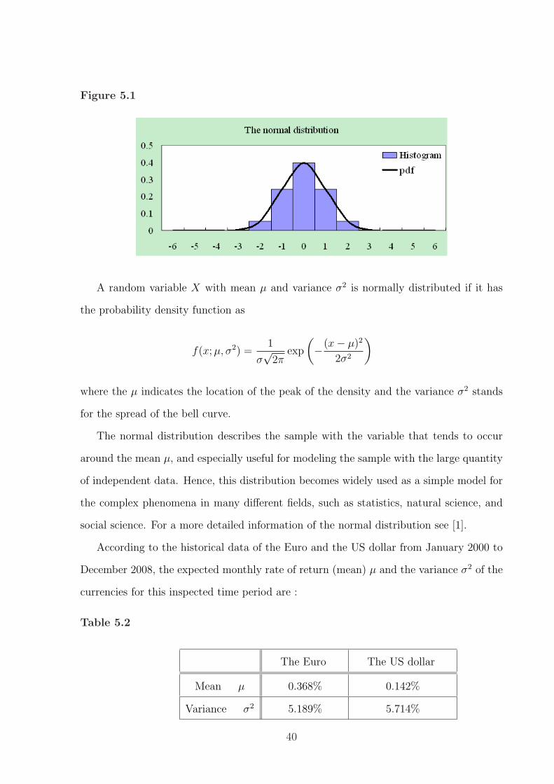
Figure 5.1

A random variable X with mean µ and variance σ2 is normally distributed if it has

the probability density function as

f(x; µ, σ2) =1

σ√

2πexp

(−(x− µ)2

2σ2

)

where the µ indicates the location of the peak of the density and the variance σ2 stands

for the spread of the bell curve.

The normal distribution describes the sample with the variable that tends to occur

around the mean µ, and especially useful for modeling the sample with the large quantity

of independent data. Hence, this distribution becomes widely used as a simple model for

the complex phenomena in many different fields, such as statistics, natural science, and

social science. For a more detailed information of the normal distribution see [1].

According to the historical data of the Euro and the US dollar from January 2000 to

December 2008, the expected monthly rate of return (mean) µ and the variance σ2 of the

currencies for this inspected time period are :

Table 5.2

The Euro The US dollar

Mean µ 0.368% 0.142%

Variance σ2 5.189% 5.714%

40

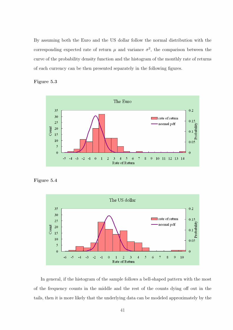
By assuming both the Euro and the US dollar follow the normal distribution with the

corresponding expected rate of return µ and variance σ2, the comparison between the

curve of the probability density function and the histogram of the monthly rate of returns

of each currency can be then presented separately in the following figures.

Figure 5.3

Figure 5.4

In general, if the histogram of the sample follows a bell-shaped pattern with the most

of the frequency counts in the middle and the rest of the counts dying off out in the

tails, then it is more likely that the underlying data can be modeled approximately by the

41

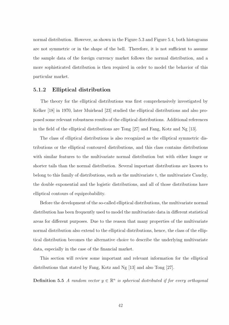
normal distribution. However, as shown in the Figure 5.3 and Figure 5.4, both histograms

are not symmetric or in the shape of the bell. Therefore, it is not sufficient to assume

the sample data of the foreign currency market follows the normal distribution, and a

more sophisticated distribution is then required in order to model the behavior of this

particular market.

5.1.2 Elliptical distribution

The theory for the elliptical distributions was first comprehensively investigated by

Kelker [18] in 1970, later Muirhead [23] studied the elliptical distributions and also pro-

posed some relevant robustness results of the elliptical distributions. Additional references

in the field of the elliptical distributions are Tong [27] and Fang, Kotz and Ng [13].

The class of elliptical distributions is also recognized as the elliptical symmetric dis-

tributions or the elliptical contoured distributions, and this class contains distributions

with similar features to the multivariate normal distribution but with either longer or

shorter tails than the normal distribution. Several important distributions are known to

belong to this family of distributions, such as the multivariate t, the multivariate Cauchy,

the double exponential and the logistic distributions, and all of those distributions have

elliptical contours of equiprobability.

Before the development of the so-called elliptical distributions, the multivariate normal

distribution has been frequently used to model the multivariate data in different statistical

areas for different purposes. Due to the reason that many properties of the multivariate

normal distribution also extend to the elliptical distributions, hence, the class of the ellip-

tical distribution becomes the alternative choice to describe the underlying multivariate

data, especially in the case of the financial market.

This section will review some important and relevant information for the elliptical

distributions that stated by Fang, Kotz and Ng [13] and also Tong [27].

Definition 5.5 A random vector y ∈ Rn is spherical distributed if for every orthogonal

42

matrix O ∈ Rn×n

Oyd= y

where the symbol p d=y denotes the equality of the distributions.

In addition, the term Y ∼ Sn(φ) is used to denote the random vector y ∈ Rn if the

vector y is spherically distributed with the characteristic generator φ. On the other hand,

if the random vector y ∈ Rn is spherically distributed with the density generator g(yT y),

then the notation Y ∼ Sn(g) will be applied instead of Y ∼ Sn(φ).

Definition 5.6 A random vector x ∈ Rn with parameters µ ∈ Rn and Σ ∈ Rn×n is

elliptically distributed if

xd= µ + AT Y

where Y ∈ Rk is spherically distributed with the characteristic generator φ, A ∈ Rk×n

with AT A = Σ, and rank(Σ) = k.

Furthermore, the corresponding notation that designates a random vector x ∈ Rn has

the elliptical distribution with the characteristic generator φ and parameters µ ∈ Rn and

Σ ∈ Rn×n is X ∼ ECn(µ, Σ, φ).

Generally, an elliptically distributed random vector x ∈ Rn does not necessarily possess

a probability density function. However, if there is a probability density function for the

elliptically distributed random vector x ∈ Rn, then the necessary condition rank(Σ) = n

must be fulfilled. And the density function of the elliptically distributed random vector

x ∈ Rn is of the form

fµ,Σ(x) = |Σ|− 12 g

((x− µ)T Σ−1(x− µ)

)

where g : R→ [0,∞) is the nonincreasing density generator.

43

As mentioned earlier in this section, there are several distributions belong to the family

of the elliptical distributions. And by considering the density generator g in the following

form for x ∈ R

g(x) = (2π)−n2 exp−

12x,

the multivariate normal distribution can be proven to be one of the elliptical distributions

as well.

Some useful results of the elliptical distributions will be summarized in the following

remark.

Remark 5.7

• If x ∼ ECn(µ, Σ, φ) and rank(Σ) = k, then the elliptically distributed random vector

x ∈ Rn has a stochastic representation

xd= µ + rAT µ(k)

with AT A = Σ and r ≥ 0 being independent of µ(k), where µ(k) denotes a random

vector that distributed uniformly on the unit sphere surface in R.

• If a distribution belongs to the family of the elliptical distributions, then all of its

marginal and conditional distributions belong to this family, furthermore, any linear

transformation of the elliptically distributed random vector x is again elliptically

distributed. And all of those results for the elliptical distributions also apply to the

multivariate normal distribution.

• If xi ∼ ECS(µ, Σ, φ) is independent and identically distributed for i = 1, 2, · · · , S,

then

Z =S∑

i=1

xi ∼ ECS(Sµ, Σ, φS)

44

with φS =∏S

i=1 φ.

5.2 Estimations of the parameters

General speaking, once a statistical distribution has been selected for describing the

underlying sample, the next approach is to estimate the parameters of the chosen distri-

bution for the optimization problem.

The maximum likelihood estimator (MLE) is considered as one of the more robust

parameter estimators, and hence widely applied in most of the practical applications.

Except the maximum likelihood estimator, there are quite a few different choices of the

parameter estimator. For example, Jorion [17] suggested to use the Bayesian estimators

which combine the traditional parameter estimator together with the external prior in-

formation, and on the other hand, Jobson and Korkie [16] proposed that the more stable

results can be achieved by using the Stein-type estimator.

This section will only consider and discuss the maximum likelihood estimator as the

estimator for the mean and the covariance matrix, and the fundamental conception behind

the maximum likelihood estimator is to determine the most likely values of the parameters

that will best describe the sample data for a given distribution. That is, let x be a random

variable with the probability density function

f(x; θ1, θ2, · · · , θn)

where θ1, θ2, · · · , θn are the parameters that need to be estimated, and the maximum

likelihood estimators of θ1, θ2, · · · , θn are obtained by maximizing the likelihood function

L(θ) = L(θ1, θ2, · · · , θn|x) = f(x; θ1, θ2, · · · , θn).

Furthermore, if the likelihood function is differentiable, then the maximum likelihood

45

estimator can be obtained by solving the maximum likelihood equation

d

dθln L(θ) = 0.

Recall the definition of the normal distribution, a random variable X is normally

distributed, X ∼ N(µ, σ2), if it has the probability density function

f(x; µ, σ2) =1

σ√

2πexp

(−(x− µ)2

2σ2

)

with mean µ and variance σ2. And by consider a set of random variables from the normal

distribution based on a random sample of size n, Xi ∼ N(µ, σ2), the corresponding

probability density function is

f(x1, x2, · · · , xn; µ, σ2) =(2πσ2

)−n2 exp

(−

∑ni=1(xi − µ)2

2σ2

)

and the likelihood function is

L(µ, σ2) = f(x1, x2, · · · , xn; µ, σ2)

=(2πσ2

)−n2 exp

(−

∑ni=1(xi − µ)2

2σ2

)

In this distribution, there are only two parameters need to be considered, the mean µ and

the variance σ2, and the value of the maximum likelihood estimator for each parameters

can be verified by solving the maximum likelihood equation with respect to the particular

parameter. The maximum likelihood equation for the parameter µ is

46

0 =d

dµln L(µ, σ2)

=d

dµln

((2πσ2

)−n2 exp

(−

∑ni=1(xi − µ)2

2σ2

))

=d

dµ

(ln

(2πσ2

)−n2 −

∑ni=1(xi − µ)2

2σ2

)

= 0− −2∑n

i=1(xi − µ)

2σ2

=2∑n

i=1(xi − µ)

2σ2

Hence, the maximum likelihood estimator for the parameter µ is

µML = x =

∑ni=1 xi

n.

Similarly, the maximum likelihood estimator of the parameter σ2 can be obtained by

setting σ2 = θ.

0 =d

dσ2ln L(µ, σ2)

=d

dθln L(µ, θ)

=d

dθln

((2πθ)−

n2 exp

(−

∑ni=1(xi − µ)2

2θ

))

=d

dθ

(ln (2πθ)−

n2 −

∑ni=1(xi − µ)2

2θ

)

=d

dθ

(constant− n

2ln θ −

∑ni=1(xi − µ)2

2θ

)

= − n

2θ+

∑ni=1(xi − µ)2

2θ2

= − nθ

2θ2+

∑ni=1(xi − µ)2

2θ2

Equivalently,

nθ =n∑

i=1

(xi − µ)2

47

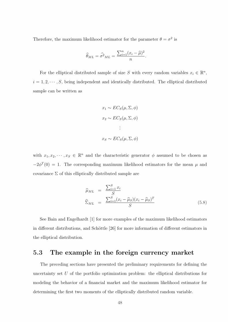
Therefore, the maximum likelihood estimator for the parameter θ = σ2 is

θML = σ2ML =

∑ni=1(xi − µ)2

n.

For the elliptical distributed sample of size S with every random variables xi ∈ Rn,

i = 1, 2, · · · , S, being independent and identically distributed. The elliptical distributed

sample can be written as

x1 ∼ ECS(µ, Σ, φ)

x2 ∼ ECS(µ, Σ, φ)

...

xS ∼ ECS(µ, Σ, φ)

with x1, x2, · · · , xS ∈ Rn and the characteristic generator φ assumed to be chosen as

−2φT (0) = 1. The corresponding maximum likelihood estimators for the mean µ and

covariance Σ of this elliptically distributed sample are

µML =

∑Si=1 xi

S

ΣML =

∑Si=1(xi − µS)(xi − µS)T

S(5.8)

See Bain and Engelhardt [1] for more examples of the maximum likelihood estimators

in different distributions, and Schottle [26] for more information of different estimators in

the elliptical distribution.

5.3 The example in the foreign currency market

The preceding sections have presented the preliminary requirements for defining the

uncertainty set U of the portfolio optimization problem: the elliptical distributions for

modeling the behavior of a financial market and the maximum likelihood estimator for

determining the first two moments of the elliptically distributed random variable.

48

By considering the same foreign currency market example that has been discussed

earlier in this paper, there are some notations need to be stated beforehand.

First of all, recall that the example of the foreign currency market consists only two

foreign currencies, the Euro and the US dollar, and the historical data from January 2000

to December 2008 for the currencies will be adopted for calculating the corresponding

parameters. This example uses the monthly rate of return of the exchange rate as the

input sources instead of the exchange rates of the currencies.

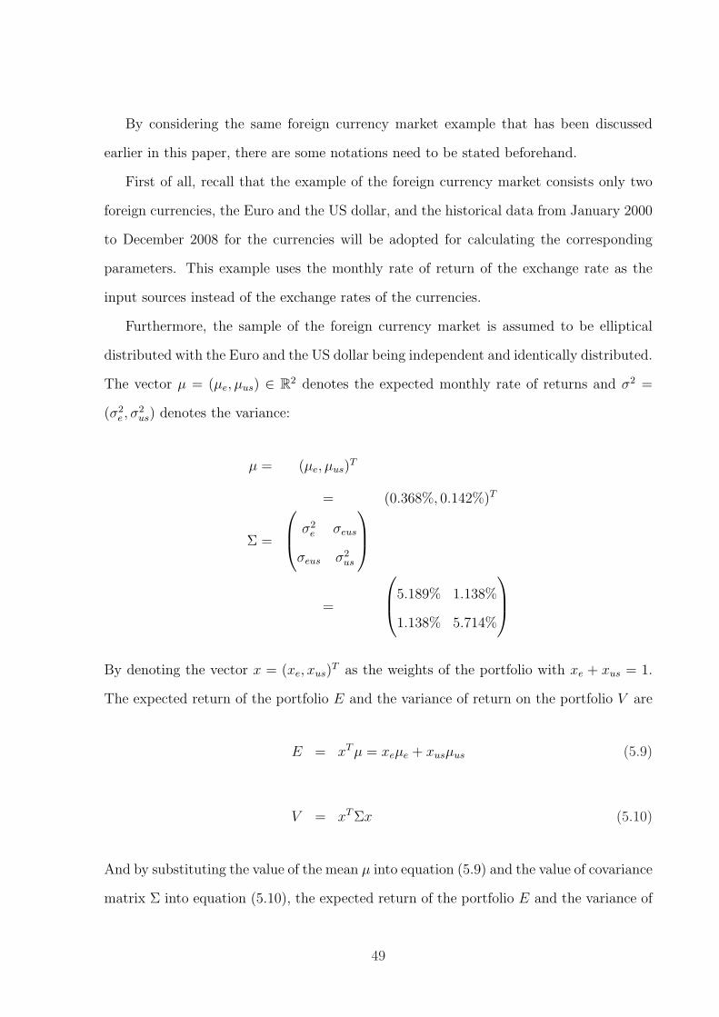
Furthermore, the sample of the foreign currency market is assumed to be elliptical

distributed with the Euro and the US dollar being independent and identically distributed.

The vector µ = (µe, µus) ∈ R2 denotes the expected monthly rate of returns and σ2 =

(σ2e , σ

2us) denotes the variance:

µ = (µe, µus)T

= (0.368%, 0.142%)T

Σ =

σ2e σeus

σeus σ2us

=

5.189% 1.138%

1.138% 5.714%

By denoting the vector x = (xe, xus)T as the weights of the portfolio with xe + xus = 1.

The expected return of the portfolio E and the variance of return on the portfolio V are

E = xT µ = xeµe + xusµus (5.9)

V = xT Σx (5.10)

And by substituting the value of the mean µ into equation (5.9) and the value of covariance

matrix Σ into equation (5.10), the expected return of the portfolio E and the variance of

49

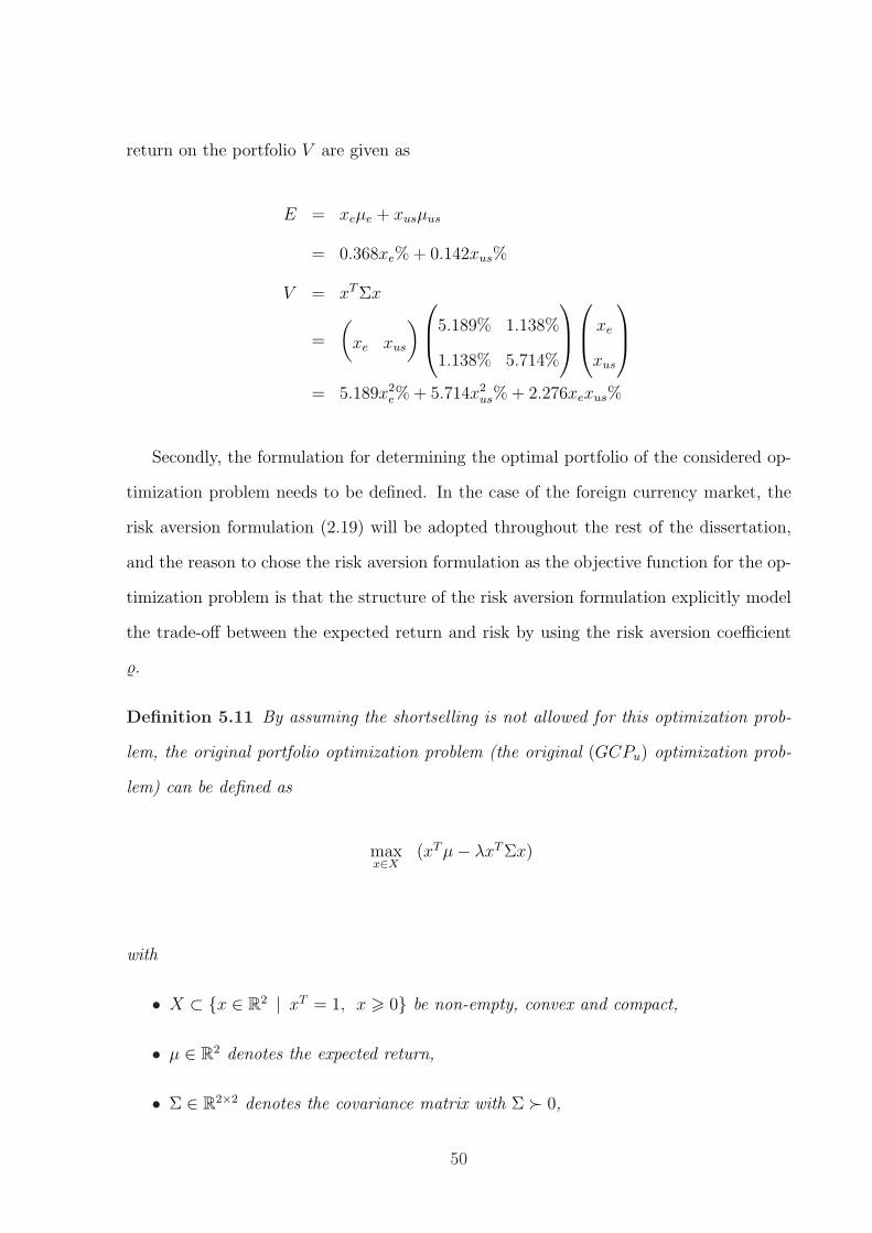
return on the portfolio V are given as

E = xeµe + xusµus

= 0.368xe% + 0.142xus%

V = xT Σx

=

(xe xus

)

5.189% 1.138%

1.138% 5.714%

xe

xus

= 5.189x2e% + 5.714x2

us% + 2.276xexus%

Secondly, the formulation for determining the optimal portfolio of the considered op-

timization problem needs to be defined. In the case of the foreign currency market, the

risk aversion formulation (2.19) will be adopted throughout the rest of the dissertation,

and the reason to chose the risk aversion formulation as the objective function for the op-

timization problem is that the structure of the risk aversion formulation explicitly model

the trade-off between the expected return and risk by using the risk aversion coefficient

%.

Definition 5.11 By assuming the shortselling is not allowed for this optimization prob-

lem, the original portfolio optimization problem (the original (GCPu) optimization prob-

lem) can be defined as

maxx∈X

(xT µ− λxT Σx)

with

• X ⊂ {x ∈ R2 | xT = 1, x > 0} be non-empty, convex and compact,

• µ ∈ R2 denotes the expected return,

• Σ ∈ R2×2 denotes the covariance matrix with Σ Â 0,

50

• % > 0 denotes the risk aversion coefficient.

Remark 5.12 Note that, the original (GCPu) optimization problem reduces to the ex-

pected return maximizing optimization problem (2.18) as the risk aversion coefficient

% = 0, and conversely, when the coefficient % is large, the original (GCPu) optimization

problem becomes to concern mostly the risk of the investment rather than the expected

return.

Strictly speaking, the mean µ and the covariance matrix Σ are the only possible

uncertain parameters for the mean variance optimization problem. Therefore, the pair

(µ, Σ) is supposed to be the uncertain parameter u for the original (GCPu) optimization

problem. However, the uncertainty set is usually defined only for the mean µ in most

of the practical cases, and the reason of that is the covariance matrix Σ behaves as a

less volatile and also less effective parameter for the mean variance optimization problem

compared to the mean µ.

Definition 5.13 The formulation for the local robust counterpart of the original (GCPu)

optimization problem is

maxx∈X

minv∈Uδ(µ)

(xT v − λxT Σx)

with

• X ⊂ {x ∈ R2 | xT = 1, x > 0} be non-empty, convex and compact,

• Uδ(µ) denotes an uncertainty set centered at point µ with the ratio of size δ > 0,

• % > 0 denotes the risk aversion coefficient.

Next, to complete the formulation for the local robust counterpart of the original

(GCPu) optimization problem, an explicit description of the uncertainty set has to be

made. As mentioned before, the form and structure of the uncertainty set U can be varied

51

depend on different requirements or concerns on future values of certain parameters. For

instance, Tutuncu and Koenig [28] preferred the interval uncertainty set that obtained by

using the bootstrapping strategies and also the moving averages of returns. On the other

hand, Ben-Tal and Nemirovski [3] and Schottle [26] proposed to solve the optimization

problem with the ellipsoidal uncertainty set. And Goldfarb and Iyengar [15] considered a

linear factor model for the multivariate returns of assets and defined the uncertainty set

by using both interval and ellipsoidal uncertainty sets. However, despite all those possible

options for defining the uncertainty set, the ellipsoidal uncertainty set is more intuitive

to apply in the optimization problem by considering a respective point estimate as the

center of the uncertainty set with the related covariance matrix and the desired level of

confidence that denote the shape and the size respectively.

For the sample of the foreign currency market, the uncertainty set Uδ(µ) can be con-

structed by choosing the maximum likelihood estimator for the mean µ, µML, as the

center of the ellipsoidal uncertainty set with the covariance matrix Σ and the ratio of size

δ > 0.

To be more specified, the maximum likelihood estimator µML is elliptically distributed

based on the independent and identically distributed random vectors µ = (µe, µus). That

is, by equation (5.8) the maximum likelihood estimator µML is

µML =µe + µus

2

and according to remark 5.7, the distribution of the maximum likelihood estimator µML

is

µML =1

2(µe + µus) ∼ EC2(2µ, Σ, φ2)

Equivalently,

µML ∼ EC2(µ,1

2Σ, φ2) (5.14)

52

By applying the definition of an ellipsoidal set1, the uncertainty set U(µ) can be displayed

as

U(µ) = {v ∈ R2 | (v − E[µML])T (Cov[µML])−1(v − E[µML]) 6 δ2}

and by substituting (5.14), the uncertainty set U(µ) is in the form of

U(µ) = {v ∈ R2 | 2(v − µ)T Σ−1(v − µ) 6 δ2} (5.15)

with δ2 denotes the desired level of confidence, µ = (0.368%, 0.142%) and Σ =

5.189% 1.138%

1.138% 5.714%

.

Alternatively, the uncertainty set U(µ) can also be expressed as

U(µ) = {v ∈ R2 | v = µ +δ√2Σ

12 w, ‖w‖ 6 1} (5.16)

by introducing a vector w ∈ R2 with

w =

√2

δΣ− 1

2 (v − µ) and wT w = ‖w‖2 = 1.

Note that, the formulation for the local robust counterpart of the original (GCPu)

optimization problem can be rearranged by applying the uncertainty set U(µ)δ stated in

(5.16). That is,

maxx∈X

minv∈Uδ(µ)

(xT v − λxT Σx

)

1An ellipsoidal set in Rn is defined as

ε = {x ∈ Rn | (x− xc)T A−1(x− xc) 6 1}

The vector xc ∈ Rn denotes the center of the ellipsoid and the matrix A = AT Â 0 denotes the distancethat the ellipsoid extends in every direction from xc.

53

by substituting v = µ + δ√2Σ

12 w

= maxx∈X min‖w‖61

(xT

(µ + δ√

2Σ

12 w

)− λxT Σx

)

= maxx∈X min‖w‖61

(xT µ + δ√

2xT Σ

12 w − λxT Σx

)

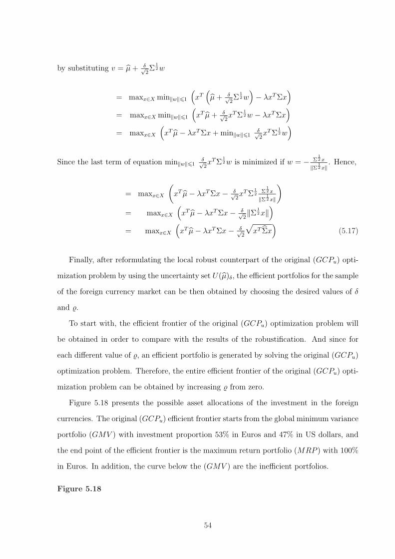
= maxx∈X

(xT µ− λxT Σx + min‖w‖61

δ√2xT Σ

12 w

)

Since the last term of equation min‖w‖61δ√2xT Σ

12 w is minimized if w = − Σ

12 x

‖Σ 12 x‖

. Hence,

= maxx∈X

(xT µ− λxT Σx− δ√

2xT Σ

12

Σ12 x

‖Σ 12 x‖

)

= maxx∈X

(xT µ− λxT Σx− δ√

2‖Σ 1

2 x‖)

= maxx∈X

(xT µ− λxT Σx− δ√

2

√xT Σx

)(5.17)

Finally, after reformulating the local robust counterpart of the original (GCPu) opti-

mization problem by using the uncertainty set U(µ)δ, the efficient portfolios for the sample

of the foreign currency market can be then obtained by choosing the desired values of δ

and %.

To start with, the efficient frontier of the original (GCPu) optimization problem will

be obtained in order to compare with the results of the robustification. And since for

each different value of %, an efficient portfolio is generated by solving the original (GCPu)

optimization problem. Therefore, the entire efficient frontier of the original (GCPu) opti-

mization problem can be obtained by increasing % from zero.

Figure 5.18 presents the possible asset allocations of the investment in the foreign

currencies. The original (GCPu) efficient frontier starts from the global minimum variance

portfolio (GMV ) with investment proportion 53% in Euros and 47% in US dollars, and

the end point of the efficient frontier is the maximum return portfolio (MRP ) with 100%

in Euros. In addition, the curve below the (GMV ) are the inefficient portfolios.

Figure 5.18

54

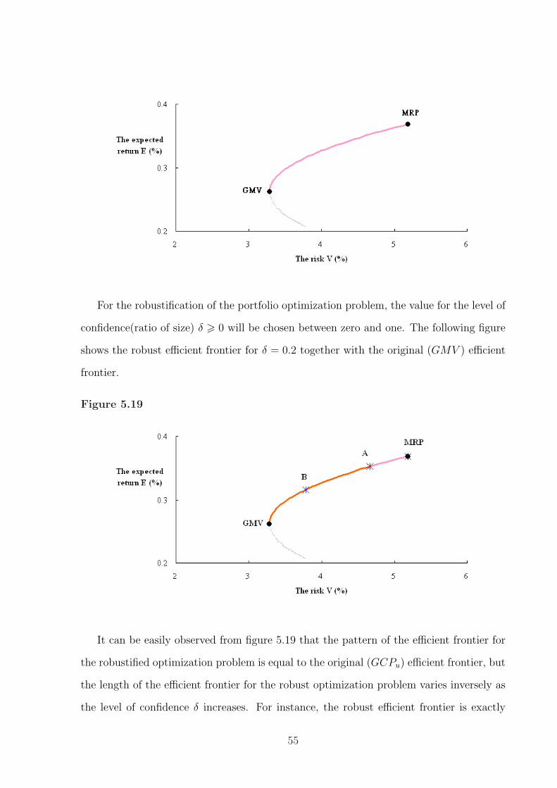
For the robustification of the portfolio optimization problem, the value for the level of

confidence(ratio of size) δ > 0 will be chosen between zero and one. The following figure

shows the robust efficient frontier for δ = 0.2 together with the original (GMV ) efficient

frontier.

Figure 5.19

It can be easily observed from figure 5.19 that the pattern of the efficient frontier for

the robustified optimization problem is equal to the original (GCPu) efficient frontier, but

the length of the efficient frontier for the robust optimization problem varies inversely as

the level of confidence δ increases. For instance, the robust efficient frontier is exactly

55

the same with the original (GCPu) efficient frontier if δ = 0.1. On the other hand, the

robust efficient frontier with δ = 0.2 begins from the point (GMV ) to point A, and for

δ = 0.3, the robust efficient frontier starts from the point (GMV ) and finished at point

B. However, except the graphical meaning that the set of efficient portfolios decreases as

the level of confidence δ increases. This phenomenon also shows that the obtained robust

optimal portfolio moves towards to the global minimum variance portfolio as the size of

the uncertainty set increases. As shown in the figure 5.20 below, for a fixed risk aversion

coefficient λ = 0.05, the robust optimal portfolios A(with δ = 0.2) and B(with δ = 0.5)

are closer to the (GMV ) portfolio than the original (GCPu) optimal portfolio.

Figure 5.20

Figure 5.21 is displayed for the purpose of showing the comparison between the optimal

portfolio allocations with the risk aversion coefficient % = 0.05. As mentioned earlier, the

robust optimal portfolio obtained by choosing a more secure uncertainty set U(µ)δ will

be more conservative, consequently, the expected return of the portfolio will be lower.

This fact can be also observed from the figure below, the investment in the US dollar

(the asset with lower variance) becomes progressively heavier as the level of confidence δ

increases. In other words, the process of applying the local robust counterpart approach

to the portfolio optimization problem can be ended up as finding the (GMV ) portfolio of

the original (GCPu) optimization problem if the level of the confidence δ is too high.

56

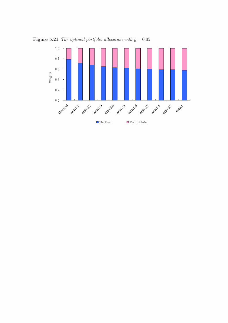
Figure 5.21 The optimal portfolio allocation with % = 0.05

Chapter 6

Conclusion

The main motivation of this dissertation is to apply the local robust counterpart

approach to the famous Markowitz mean variance portfolio optimization problem. To

enable this application, the concepts of the mean variance portfolio optimization, the

general convex conic optimization, and also the (local) robust counterpart approach have

been studied and discussed. As the purpose of this dissertation is to investigate the

process of applying the robust counterpart approach, therefore, only the related and also

necessary notions and properties were mentioned.

The robustification of an optimization problem provides more secured and stable re-

sults even if the underlying parameters are uncertain. However, as observed from the

given example of the foreign currency market, the obtained optimal portfolio can be too

conservative if the chosen uncertainty set is too large, and on the other hand, if the un-

certainty set is too small, then the robust counterpart approach will not be sufficiently to

apply for optimizing the problem.

Above all, in view of the fact that the (local) robust counterpart approach is the

methodology that optimizes the problem over the uncertainty set, therefore, explicitly

definitions and restrictions are still needed in order to characterize the uncertainty set

without eliminate the important information from the original data. Although there

are some recommended guidelines for constructing the uncertainty set for the robust

optimization problem, the investigation of how to creat an appropriate uncertainty set for

the particular optimization problem is still in progress.

59

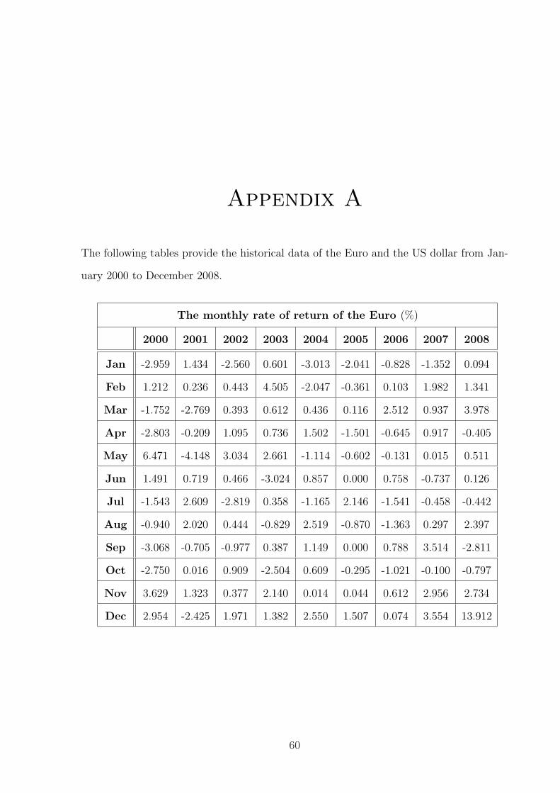
Appendix A

The following tables provide the historical data of the Euro and the US dollar from Jan-

uary 2000 to December 2008.

The monthly rate of return of the Euro (%)

2000 2001 2002 2003 2004 2005 2006 2007 2008

Jan -2.959 1.434 -2.560 0.601 -3.013 -2.041 -0.828 -1.352 0.094

Feb 1.212 0.236 0.443 4.505 -2.047 -0.361 0.103 1.982 1.341

Mar -1.752 -2.769 0.393 0.612 0.436 0.116 2.512 0.937 3.978

Apr -2.803 -0.209 1.095 0.736 1.502 -1.501 -0.645 0.917 -0.405

May 6.471 -4.148 3.034 2.661 -1.114 -0.602 -0.131 0.015 0.511

Jun 1.491 0.719 0.466 -3.024 0.857 0.000 0.758 -0.737 0.126

Jul -1.543 2.609 -2.819 0.358 -1.165 2.146 -1.541 -0.458 -0.442

Aug -0.940 2.020 0.444 -0.829 2.519 -0.870 -1.363 0.297 2.397

Sep -3.068 -0.705 -0.977 0.387 1.149 0.000 0.788 3.514 -2.811

Oct -2.750 0.016 0.909 -2.504 0.609 -0.295 -1.021 -0.100 -0.797

Nov 3.629 1.323 0.377 2.140 0.014 0.044 0.612 2.956 2.734

Dec 2.954 -2.425 1.971 1.382 2.550 1.507 0.074 3.554 13.912

60

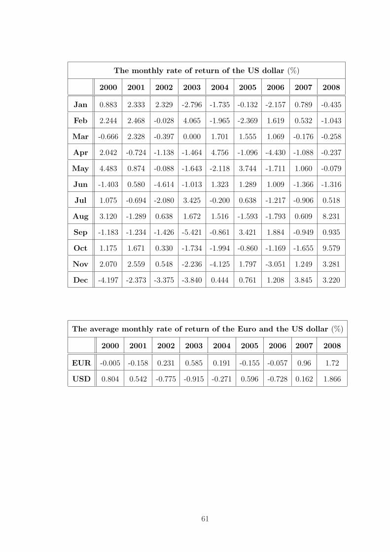
The monthly rate of return of the US dollar (%)

2000 2001 2002 2003 2004 2005 2006 2007 2008

Jan 0.883 2.333 2.329 -2.796 -1.735 -0.132 -2.157 0.789 -0.435

Feb 2.244 2.468 -0.028 4.065 -1.965 -2.369 1.619 0.532 -1.043

Mar -0.666 2.328 -0.397 0.000 1.701 1.555 1.069 -0.176 -0.258

Apr 2.042 -0.724 -1.138 -1.464 4.756 -1.096 -4.430 -1.088 -0.237

May 4.483 0.874 -0.088 -1.643 -2.118 3.744 -1.711 1.060 -0.079

Jun -1.403 0.580 -4.614 -1.013 1.323 1.289 1.009 -1.366 -1.316

Jul 1.075 -0.694 -2.080 3.425 -0.200 0.638 -1.217 -0.906 0.518

Aug 3.120 -1.289 0.638 1.672 1.516 -1.593 -1.793 0.609 8.231

Sep -1.183 -1.234 -1.426 -5.421 -0.861 3.421 1.884 -0.949 0.935

Oct 1.175 1.671 0.330 -1.734 -1.994 -0.860 -1.169 -1.655 9.579

Nov 2.070 2.559 0.548 -2.236 -4.125 1.797 -3.051 1.249 3.281

Dec -4.197 -2.373 -3.375 -3.840 0.444 0.761 1.208 3.845 3.220

The average monthly rate of return of the Euro and the US dollar (%)

2000 2001 2002 2003 2004 2005 2006 2007 2008

EUR -0.005 -0.158 0.231 0.585 0.191 -0.155 -0.057 0.96 1.72

USD 0.804 0.542 -0.775 -0.915 -0.271 0.596 -0.728 0.162 1.866

61

Appendix B

For a given pair (u, δ) with u ∈ Uδ(u) and δ > 0, the associated sets of the (LRCu,δ)

problem are:

• The feasible set FLRC(u, δ) : {x ∈ X | g(x, u) ¹K 0}.

• The optimal set F ∗LRC(u, δ) : {x ∈ FLRC(u, δ) | fLRC(x, u, δ) ≤ f ∗LRC(u, δ)}.

• The set of Slater points F SLRC(u, δ) : {x ∈ X | g(x, u) ≺K 0}.

where f ∗LRC : U × R+ → R is the optimal value function defined as

f ∗LRC(u, δ) := min{fLRC(x, u, δ) | x ∈ FLRC(u, δ)}. (6.1)

Furthermore, the corresponding functions assign the feasible set FLRC(u, δ) and the

optimal set F ∗LRC(u, δ) are

• The feasible set mapping FLRC : U × R+ →℘(X).

• The optimal set mapping F ∗LRC : U × R+ →℘(X).

62

List of References

[1] L.J. Bain and M. Engelhardt. Introduction to Probability and Mathematical Statistics.Duxbury Press, California, second edition, 2000.

[2] B. Bank. Non-linear Parametric Optimization. Birkhauser, Basel, 1983.

[3] A. Ben-Tal and A. Nemirovski. Robust convex optimization. Mathematics of Oper-ations Research, 23(4):769–805, 1998.

[4] A. Ben-Tal and A. Nemirovski. Selected topics in robust convex optimization. Math-ematical Programming, 112(1):125–158, 2008.

[5] M.J. Best and R.R. Grauer. On the sensitivity of mean-variance efficient portfoliosto changes in asset means: Some analytical and computational results. Review ofFinancial Studies, 4(2):315–342, 1991.

[6] S. Boyd and L. Vandenberghe. Convex Optimization. Cambridge University Press,2004.

[7] J. Brinkhuis and V. Tikhomirov. Optimization: Insights and Applications. PrincetonUniversity Press, New Jersey, 2005.

[8] M. Britten-Jones. The sampling error in estimates of mean-variance efficient portfolioweights. Journal of Finance, 54(2):655–671, 1999.

[9] G. Calafiore and M.C.Campi. Uncertain convex programs: randomized solutions andconfidence levels. Mathematical Programming, 102(4):25–46, 2005.

[10] G. Cornuejols and R. Tutuncu. Optimization Methods in Finance. Cambridge Uni-versity Press, Cambridge, 2007.

[11] E.J. Elton, M.J. Gruber, S.J. Brown, and W.N. Goetzmann. Modern Portfolio Theoryand Investment Analysis. John Wiley & Sons, New York, sixth edition, 2003.

[12] F.J. Fabozzi, P.N. Kolm, D.A. Pachamanova, and S.M. Focardi. Robust PortfolioOptimization and Management. John Wiley & Sons, New Jersey, 2007.

[13] K.-T. Fang, S. Kotz, and K.-W. Ng. Symmetric Multivariate and Related Distribu-tions. Chapman and Hall, London, 1990.

[14] G.M. Frankfurter, H.E. Phillips, and J.P. Seagle. Portfolio selection: The effects ofuncertain means, variances and covariances. Journal of Financial and QuantitativeAnalysis, 6:1251–1262, 1971.

63

[15] D. Goldfarb and G. Iyengar. Robust portfolio selection problems. Mathematics ofOperations Research, 28(1):1–38, 2003.

[16] J.D. Jobson and B. Korkie. Putting Markowitz theory to work. Journal of PortfolioManagement, 7(4):70–74, 1981.

[17] P. Jorion. Bayes-Stein Estimation for Portfolio Analysis. Journal of Financial andQuantitative Analysis, 21(3):279–292, 1986.

[18] D. Kelker. Distribution theory of spherical distributions and a location-scale param-eter. Sankhya : The Indian Journal of Statistics, 32(A):499–516, 1970.

[19] L. Laloux, P. Cizeau, J.P. Bouchaud, and M. Potters. Noise dressing of financialcorrelation matrices. Physical Review Letters, 83:1467–1470, 1999.

[20] H.M. Markowitz. Portfolio Selection: Efficient Diversification of investments. JohnWiley & Sons, New York, 1959.

[21] H.M. Markowitz. Mean-Variance Analysis in Portfolio Choice and Capital Markets.Blackwell, New York, 1987.

[22] R.O. Michaud. Efficient Asset Management. Harvard Business School Press, Boston,1998.

[23] R.J. Muirhead. Aspects of Multivariate Statistical Theory. John Wiley, New York,1982.

[24] J.M. Mulvey, R.J. Vanderbei, and S.A. Zenios. Robust optimization of large-scalesystems. Operations Research, 43(2):264–281, 1995.

[25] S. Pafka and I. Kondor. Estimated correlation matrices and portfolio optimization.Physica A, 343:623–634, 2004.

[26] K. Schottle. Robust Optimization with Application in Asset Management. PhD thesis,Technische Universitat Munchen, Department of Mathematics, 2007.

[27] Y.L. Tong. The Multivariate Normal Distribution. Springer-Verlag, New York, 1990.

[28] R.H. Tutuncu and M. Koenig. Robust asset allocation. Annals of Operations Re-search, 132:157–187, 2004.

64