Boundary Control of PDEs:

A Course on Backstepping Designs

class slides

Miroslav Krstic

Introduction

• Fluid flows in aerodynamics and propulsion applications;

plasmas in lasers, fusion reactors, and hypersonic vehicles;

liquid metals in cooling systems for tokamaks and computers, as well as in weldingand metal casting processes;

acoustic waves, water waves in irrigation systems...

• Flexible structures in civil engineering, aircraft wings and helicopter rotors, astronom-ical telescopes, and in nanotechnology devices like the atomic force microscope...

• Electromagnetic waves and quantum mechanical systems...

• Waves and “ripple” instabilities in thin film manufacturing and in flame dynamics...

• Chemical processes in process industries and in internal combustion engines...

Unfortunately, even “toy” PDE control problems like heat and wave equations (neither ofwhich is unstable) require some background in functional analysis.

Courses in control of PDEs rare in engineering programs.

This course: methods which are easy to understand, minimal background beyond calculus.

Boundary Control

Two PDE control settings:

• “in domain” control (actuation penetrates inside the domain of the PDE system or isevenly distributed everywhere in the domain, likewise with sensing);

• “boundary” control (actuation and sensing are only through the boundary conditions).

Boundary control physically more realistic because actuation and sensing are non-intrusive(think, fluid flow where actuation is from the walls).!

!“Body force” actuation of electromagnetic type is also possible but it has low control authority and its spatialdistribution typically has a pattern that favors the near-wall region.

Boundary control harder problem, because the “input operator” (the analog of the B matrixin the LTI finite dimensional model x= Ax+Bu) and the output operator (the analog of theC matrix in y=Cx) are unbounded operators.

Most books on control of PDEs either don’t cover boundary control or dedicate only smallfractions of their coverage to boundary control.

This course is devoted exclusively to boundary control.

Backstepping

A particular approach to stabilization of dynamic systems with “triangular” structure.

Wildly successful in the area of nonlinear control since

[KKK] Krstic, Kanellakopoulos, KokotovicNonlinear and Adaptive Control Design, 1995.

Other methods:

Optimal control for PDEs requires sol’n of operator Riccati equations (nonlinear andinfinite-dimensional algebraic eqns).

Pole placement pursues precise assignment of a finite subset of the PDE’s eigenvaluesand requires model reduction.

Instead, backstepping achieves Lyapunov stabilization by transforming the system into astable “target system.”

A Short List of Other Books on Control of PDEs

• R. F. CURTAIN AND H. J. ZWART, An Introduction to Infinite DimensionalLinear Systems Theory, Springer-Verlag, 1995.

• I. LASIECKA, R. TRIGGIANI, Control Theory for Partial Differential Equations:Continuous and Approximation Theories, Cambridge Univ. Press, 2000.

• A. BENSOUSSAN, G. DA PRATO, M. C. DELFOUR AND S. K. MITTER, Rep-resentation and control of infinite–dimensional systems, Birkhauser, 2006.

• Z. H. LUO, B. Z. GUO, AND O. MORGUL, Stability and Stabilization of InfiniteDimensional Systems with Applications, Springer Verlag, 1999.

• J. E. LAGNESE, Boundary stabilization of thin plates, SIAM, 1989.

• P. CHRISTOFIDES, Nonlinear and Robust Control of Partial Differential Equa-tion Systems: Methods and Applications to Transport-Reaction Processes,Boston: Birkhauser, 2001.

The Role of Model Reduction

Plays an important role in most methods for control design for PDEs.

They extract a finite dimensional subsystem to be controlled, while showing robustness toneglecting the remaining infinite dimensional dynamics in the design.

Backstepping does not employ model reduction—none is needed, except at the implemen-tation stage.

Control Objectives for PDE Systems

• Performance improvement—for stable systems, optimal control.

• Stabilization—this course deals almost exclusively w/ unstable plants.

• Trajectory tracking—requires stabilizing fbk plus sol’n to trajectory generation probl.

• Trajectory generation/motion planning—towards the end of the course.

Classes of PDEs and Benchmark PDEs Dealt With in the Course

In contrast to ODEs, no general methodology for PDEs.

Two basic categories of PDEs studied in textbooks: parabolic and hyperbolic PDEs, withstandard examples being heat and wave equations.

Many more categories.

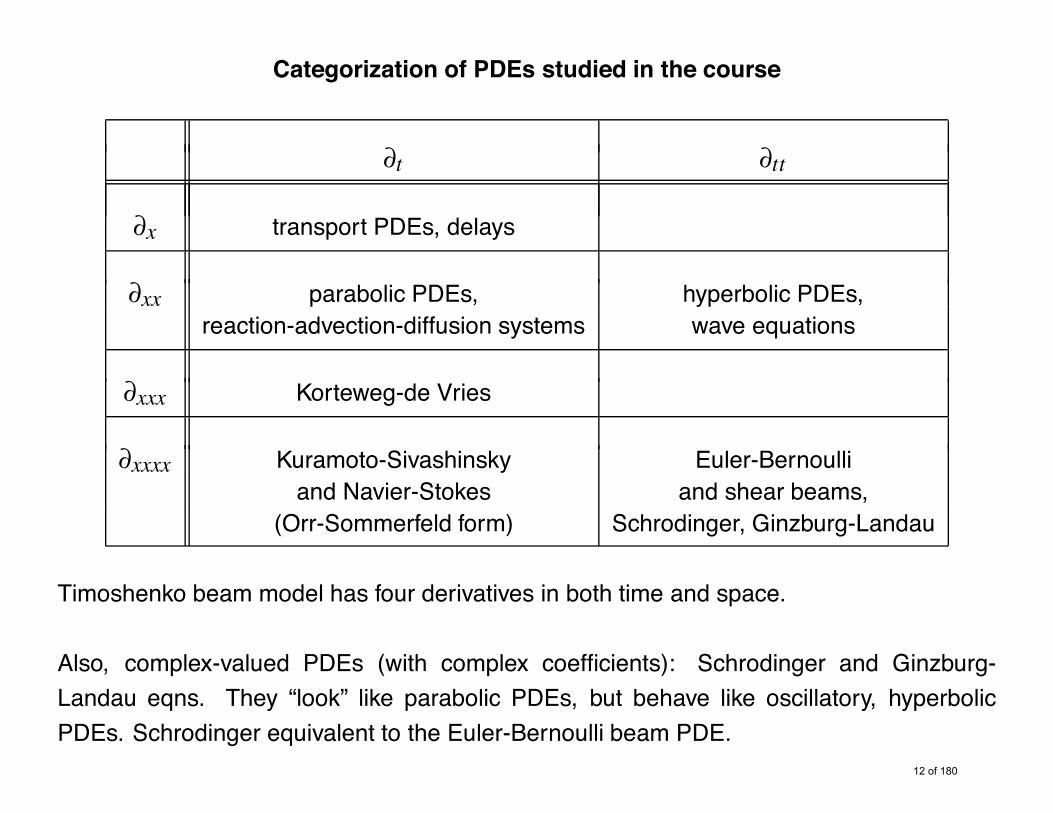
Categorization of PDEs studied in the course

!t !tt

!x transport PDEs, delays

!xx parabolic PDEs, hyperbolic PDEs,reaction-advection-diffusion systems wave equations

!xxx Korteweg-de Vries

!xxxx Kuramoto-Sivashinsky Euler-Bernoulliand Navier-Stokes and shear beams,

(Orr-Sommerfeld form) Schrodinger, Ginzburg-Landau

Timoshenko beam model has four derivatives in both time and space.

Also, complex-valued PDEs (with complex coefficients): Schrodinger and Ginzburg-Landau eqns. They “look” like parabolic PDEs, but behave like oscillatory, hyperbolicPDEs. Schrodinger equivalent to the Euler-Bernoulli beam PDE.

Choices of Boundary Controls

Thermal: actuate heat flux or temperature.

Structural: actuate beam’s boundary position, or force, or angle, or moment.

Mathematical choices of boundary control:

Dirichlet control u(1, t)—actuate value of a function at boundary

Neumann control ux(1, t)—actuate slope of a function at boundary

The Domain Dimension—1D, 2D, and 3D

PDE control complex enough in 1D: string, acoustic duct, beam, chemical tubular reactor,etc.

Can have finitely- and even infinitely-many unstable eigenvalues.

Some PDEs evolve in 2D and 3D but are dominated by phenomena evolving in one coor-dinate direction (while the phenomena in the other directions are stable and slow).

Some PDEs are genuinely 3D: Navier-Stokes.

See the companion book:

Vazquez and Krstic, Control of Turbulent and Magnetohydrodynamic ChannelFlows, Birkhauser, 2007.

Domain Shape in 2D and 3D

Rectangle or annulus much more readily tractable than a problem where the domain hasan “amorphous/wiggly” shape.

Beware: literature abounds with abstract control methods for 2D and 3D PDE systems ongeneral domains, where the complexities are hidden behind neatly written Riccati eqns.

Genuinely 2D or 3D systems, particularly if unstable and on oddly shaped domains (e.g.,turbulent fluids in 3D around irregularly shaped bodies), truly require millions of differentialequations to simulate and tens of thousands of equations to do control design for them.

Reasonable set up: boundary control of an endpoint of a line interval; edge of a rectangle;side of e parallelepiped.(Dimension of actuation domain lower by one than dimension of PDE domain.)

Observers

Observer design using boundary sensing, dual to full-state fbk boundary control design.

Observer error system is exponentially stabilized.

Separation principle holds.

Adaptive Control of PDEs

Parameter estimators—system identifiers—for PDEs.

Unstable PDEs with unknown parameters controlled using parameter estimators suppliedby identifiers and using state estimators supplied by adaptive observers.

See the companion book

Smyshlyaev and Krstic, Adaptive Control of Parabolic PDEs, Princeton UniversityPress, 2010.

Nonlinear PDEs

At present, virtually no methods exist for boundary control of nonlinear PDEs.

Several results are available that apply to nonlinear PDEs that are neutrally stable andwhere the nonlinearity plays no destabilizing role.

No advanced control designs exist for broad classes of nonlinear PDEs that are open-loopunstable and where a sophisticated control Lyapunov function of non-quadratic type needsto be constructed to achieve closed-loop stability.

Though the focus of the course is on linear PDEs, we introduce basic ideas for stabilizationof nonlinear PDEs at the end.

Delay Systems

A special class of ODE/PDE systems.

Delay is a transport PDE. (One derivative in space and one in time. First-order hyperbolic.)

Specialized books by Gu, Michiels, Niculescu.

A book focused on input delays, nonlinear plants, and unknown delays:

M. Krstic, Delay Compensation for Nonlinear, Adaptive, and PDE Systems,Birkhauser, 2009.

Organization of the Course

1. Basic Lyapunov stability ideas for PDEs. Backstepping transforms a PDE into a desir-able “target PDE” within the same class. General Lyapunov thms for PDEs not veryuseful. We learn how to calculate stability estimates for a basic stable PDE and high-light the roles of spatial norms (L2, H1, and so on), the role of the Poincare, Agmon,and Sobolev inequalities, the role of integration by parts in Lyapunov calculations, andthe distinction between energy boundedness and pointwise (in space) boundedness.

2. Eigenvalues, eigenfunctions, and basics of finding solutions of PDEs analytically.

3. Backstepping method. Our main “tutorial tool” is the reaction-diffusion PDE example

ut(x, t) = uxx(x, t)+"u(x, t) ,

on the spatial interval x " (0,1), with one uncontrolled boundary condition at x= 0,

u(0, t) = 0

and with a control applied through Dirichlet boundary actuation at x= 1.

4. Observer design. Develop a dual of backstepping for finding observer gain functions.Use reaction-diffusion PDE as an example.

5. Schrodinger and Ginzburg-Landau PDEs. Complex-valued but a backstepping designfor parabolic PDEs easily extended. GL models vortex shedding.

6. Hyperbolic and “hyperbolic-like” equations—wave equations, beams, transport equa-tions, and delay equations.

7. “Exotic” PDEs, with just one time derivative but with three and even four spatialderivatives—Kuramoto-Sivashinsky and Korteweg-de Vries eqns.

8. 3D Navier-Stokes eqn at high Reynolds number.

9. Motion planning/trajectory generation for PDEs. For example, how to find the timefunction for the input force for one end of a flexible beam to produce precisely thedesired time-varying motion with the tip of the free end of the beam.

10. Adaptive control for parametrically uncertain PDEs.

11. Nonlinear PDEs.

Why We Don’t State Theorems

Focus on tools that allow to solve many problems, rather than on developing completetheorem statements for a few problems.

Want to move fast and cover many classes of PDEs and control/estimation topics.

Want to maintain physical intuition.

Want to make the material accessible to any control engineering grad student.

Focus on Unstable PDEs in 1D and Feedback Design Challenges

Unstable parabolic and hyperbolic PDEs in 1D with terms causing instability unmatchedby the boundary control.

Feedback design challenges greater than the existence/uniqueness challenges, which arewell addressed in analysis-oriented PDE books.

The Main Idea of Backstepping Control

Backstepping is a robust† extension of the “feedback linearization” approach for nonlinearfinite-dimensional systems.

†Backstepping provides design tools that endow the controller with robustness to uncertain parameters andfunctional uncertainties in the plant nonlinearities, and robustness to external disturbances, robustness toother forms of modeling errors.

Feedback linearization entails two steps:

1. Construction of an invertible change of variables such that the system appears aslinear in the new variables, except for a nonlinearity which is “in the span” of thecontrol input vector;

2. Cancellation of the nonlinearity‡ and the assignment of desirable linear exponentiallystable dynamics on the closed-loop system.

‡In contrast to the standard feedback linearization, backstepping allows the flexibility to not necessarilycancel the nonlinearity. A nonlinearity may be kept if it is useful or it may be dominated (rather thancancelled non-robustly) if it is potentially harmful and uncertain.

Backstepping for PDEs:

1. Identify the undesirable terms in the PDE.

2. Choose a target system in which the undesirable terms are to be eliminated by statetransformation and feedback, as in feedback linearization.

3. Find the state transformation as identity minus a Volterra operator (in x).Volterra operator = integral operator from 0 up to x (rather than from 0 to 1).Volterra transformation is “triangular” or “spatially causal.”

4. Obtain boundary feedback from the Volterra transformation. The transformation alonecannot eliminate the undesirable terms, but the transformantion brings them to theboundary, so control can cancel them.

Gain fcn of boundary controller = kernel of Volterra transformation.

Volterra kernel satisfies a linear PDE.

Backstepping is not “one-size-fits-all.” Requires structure-specific effort by designer.

Reward: elegant controller, clear closed-loop behavior.

Unique to This Course—Elements of Adaptive and Nonlinear Designs for PDEs

Prior to backstepping, state-of-the-art in adaptive and nonlinear control for PDEs compa-rable to the state-of-the-art for ODEs in the 1960s.

A wide range of PDE structures with nonlinearities, unknown parameters, and boundarycontrol require backstepping.

Origins of This Course

Developed out of research results and papers by the instructor and his PhD students.

First taught as MAE 287 Distributed Parameter Systems at University of California, SanDiego, in Fall 2005.

Lyapunov Stability

Recall some basics of stability analysis for linear ODEs.

An ODE

z= Az , z " Rn (1)

is exponentially stable (e.s.) at z = 0 if #M > 0 (overshoot coeff.) and # > 0 (decay rate)s.t.

$z(t)$ %Me&#t$z(0)$, for all t ' 0 (2)

$ ·$ denotes one of the equivalent vector norms, e.g., the 2-norm.

This is a definition of stability. If all the eigenvalues of the matrix A have negative real parts,this guarantees e.s., but this test is not always practical.

An alternative (iff) test which is more useful in state-space/time-domain and robustnessstudies:

( positive definite n) n matrix Q, # a positive definite and symmetric matrix Ps.t.

PA+ATP= &Q . (3)

Lyapunov function:

V = xTPx , positive definite (4)V = &xTQx , negative definite . (5)

For PDEs, an (infinite-dimensional) operator equation like (3) is hard to solve.

Key question for PDEs: not Lyapunov functions but system norms!

In finite dimension, vector norms are “equivalent.” No matter which norm $ ·$ one uses in(2) (for example, the 2-norm, 1-norm, or $-norm) one gets e.s. in the sense of any othervector norm. What changes are the constants M and # in (2).

For PDEs, the state space is not a Euclidean space but a function space, and likewise, thestate norm is not a vector norm but a function norm.

Unfortunately, norms on function spaces are not equivalent. Bounds on the state in termsof the L1, L2, or L$ norm in x do not follow from one another.

To make matters more complicated, other natural choices of state norms for PDEs existwhich are not equivalent with Lp norms. Those are the Sobolev norms, examples of whichare the H1 and H2 norms (not to be confused with Hardy space norms in robust controlfor ODE systems), which, roughly, are the L2 norms of the first and second derivative,respectively, of the PDE state.

With such a variety of choice, dictated by idiosyncracies of the PDE classes, general Lya-punov stability theory for PDEs is hopeless, though some efforts are made in

1. J. A. WALKER, Dynamical Systems and Evolution Equations, Plenum, 1980.

2. D. HENRY, Geometric Theory of Semilinear Parabolic Equations, Springer, 1993.

Instead, one is better off learning how to derive, from scratch, “energy estimates” (one’sown Lyapunov theorems) in different norms.

A Basic PDE Model

Before introducing stability concepts, we develop a basic “non-dimensionalized” PDEmodel, a 1D heat equation, which will help introduce the idea of energy estimates now,and be used as a target system for some backstepping designs later.

%

A thermally conducting rod.

The evolution of the temperature profile T (%,&), as a function of the spatial variable % andtime &, is described by the heat equation§

T&(%,&) = 'T%%(%,&) , x " (0,L) (6)T (0,&) = T1 , left end of rod (7)T (L,&) = T2 , right end of rod (8)T (%,0) = T0(%) , initial temperature distribution . (9)

' = thermal diffusivityT&, T%% = partial derivatives with respect to time and space.

§While in physical heat conduction problems it is more appropriate to assume that the heat flux T% is heldconstant at the boundaries (rather than the temperature T itself), for simplicity of our introductory expositionwe proceed with the boundary conditions as in (7), (8)

Our objective is to write this equation in nondimensional variables that describe the errorbetween the unsteady temperature and the equilibrium profile of the temperature:

1. Scale % to normalize length:

x=%L

, (10)

which gives

T&(x,&) ='L2Txx(x,&) (11)

T (0,&) = T1 (12)T (1,&) = T2 . (13)

2. Scale time to normalize thermal diffusivity:

t ='L2

& , (14)

which gives

Tt(x, t) = Txx(x, t) (15)T (0, t) = T1 (16)T (1, t) = T2 . (17)

3. Introduce new variable

w= T & T (18)

where

T (x) = T1+ x(T2&T1)

is the steady-state profile and is found as a solution to the two-point boundary-valueODE

T **(x) = 0 (19)T (0) = T1 (20)T (1) = T2 . (21)

We obtain

wt = wxx (22)w(0) = 0 (23)w(1) = 0 , (24)

with initial distribution w0 = w(x,0).

Note that here and throughout the rest of the course for compactness and ease of the presentation we drop

the dependence on time and spatial variable where it does not lead to a confusion, i.e. by w, w(0) we always

mean w(x, t), w(0, t), respectively, unless specifically stated.

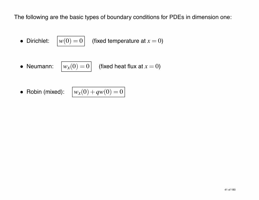
The following are the basic types of boundary conditions for PDEs in dimension one:

• Dirichlet: w(0) = 0 (fixed temperature at x= 0)

• Neumann: wx(0) = 0 (fixed heat flux at x= 0)

• Robin (mixed): wx(0)+qw(0) = 0

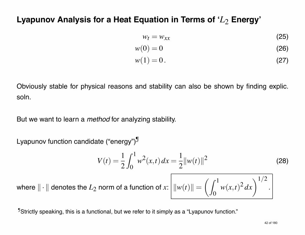
Lyapunov Analysis for a Heat Equation in Terms of ‘L2 Energy’

wt = wxx (25)w(0) = 0 (26)w(1) = 0 . (27)

Obviously stable for physical reasons and stability can also be shown by finding explic.soln.

But we want to learn a method for analyzing stability.

Lyapunov function candidate (“energy”)¶

V (t) =12

Z 1

0w2(x, t)dx=

12$w(t)$2 (28)

where $ ·$ denotes the L2 norm of a function of x: $w(t)$ =

!Z 1

0w(x, t)2dx

"1/2.

¶Strictly speaking, this is a functional, but we refer to it simply as a “Lyapunov function.”

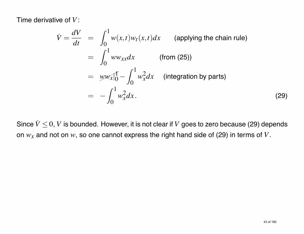
Time derivative of V :

V =dVdt

=Z 1

0w(x, t)wt(x, t)dx (applying the chain rule)

=Z 1

0wwxxdx (from (25))

=!

!!

!!!

wwx|10&Z 1

0w2xdx (integration by parts)

= &Z 1

0w2xdx . (29)

Since V % 0,V is bounded. However, it is not clear ifV goes to zero because (29) dependson wx and not on w, so one cannot express the right hand side of (29) in terms of V .

Recall two useful inequalities:

Young’s Inequality (special case)

ab%(2a2+

12(b2 (30)

Cauchy-Schwartz Inequality

Z 1

0uwdx%

!Z 1

0u2dx

"1/2!Z 1

0w2dx

"1/2(31)

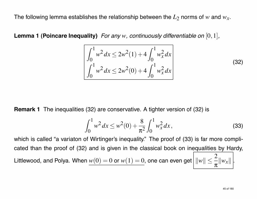
The following lemma establishes the relationship between the L2 norms of w and wx.

Lemma 1 (Poincare Inequality) For any w, continuously differentiable on [0,1],Z 1

0w2dx% 2w2(1)+4

Z 1

0w2x dx

Z 1

0w2dx% 2w2(0)+4

Z 1

0w2x dx

(32)

Remark 1 The inequalities (32) are conservative. A tighter version of (32) isZ 1

0w2dx% w2(0)+

8)2

Z 1

0w2x dx , (33)

which is called “a variaton of Wirtinger’s inequality.” The proof of (33) is far more compli-cated than the proof of (32) and is given in the classical book on inequalities by Hardy,

Littlewood, and Polya. When w(0) = 0 or w(1) = 0, one can even get $w$ %2)$wx$ .

Proof.Z 1

0w2dx = xw2|10&2

Z 1

0xwwx dx (integration by parts)

= w2(1)&2Z 1

0xwwxdx

% w2(1)+12

Z 1

0w2dx+2

Z 1

0x2w2x dx .

Subtracting the second term from both sides we get the first inequality in (32):

12

Z 1

0w2dx % w2(1)+2

Z 1

0x2w2xdx

% w2(1)+2Z 1

0w2xdx . (34)

The second inequality in (32) is obtained in a similar fashion. QED

We now return to

V = &Z 1

0w2xdx .

Using Poincare inequality along with boundary conditions w(0) = w(1) = 0, we get

V = &Z 1

0w2xdx%&

14

Z 1

0w2 %&

12V (35)

which, by the basic comparison principle for first order differential inequalities, implies that

V (t) %V (0)e&t/2, (36)

or

$w(t)$ % e&t/4$w0$ (37)

Thus, the system (25)–(27) is exponentially stable in L2.

xt

w(x, t)

Response of a heat equation to a non-smooth initial condition.

The “instant smoothing” effect is the characteristic feature of the diffusion operator thatdominates the heat equation.

Pointwise-in-Space Boundedness and Stability in Higher Norms

We established that

$w$ + 0 as t + $

but this does not imply that w(x, t) goes to zero for each x " (0,1).

Are there “unbounded spikes” for some x along the spatial domain (on a set ofmeasure zero) which do not contribute to the L2 norm?

It would be desirable to show that

maxx"[0,1]

|w(x, t)|% e&t4 maxx"[0,1]

|w(x,0)| , (38)

namely, stability in the spatial L$ norm. But this is possible only in some special cases andnot worth our attention in a course that focuses on basic but generally applicable tools.

However, it is easy to show a more restrictive result than (38), given by

maxx"[0,1]

|w(x, t)|% Ke&t2$w0$H1 (39)

for some K > 0, where the H1 norm is defined by

$w$2H1 :=

#Z 1

0w2dx+

Z 1

0w2xdx (40)

Remark 2 The H1 norm can be defined in different ways, the definition given above suitsour needs. Note also that by using the Poincare inequality, it is possible to drop the firstintegral in (40) for most problems.

Before we proceed to prove (39), we need the following result.

Lemma 2 (Agmon’s Inequality) For a function w "H1, the following inequalities hold

maxx"[0,1]

|w(x, t)|2 % w(0)2+2$w(t)$$wx(t)$

maxx"[0,1]

|w(x, t)|2 % w(1)2+2$w(t)$$wx(t)$(41)

Proof.Z x

0wwxdx=

Z x

0!x12w2dx

=12w2|x0

=12w(x)2&

12w(0)2. (42)

Taking the absolute value on both sides and using the triangle inequality gives

12|w(x)2|%

Z x

0|w||wx|dx+

12w(0)2. (43)

Using the fact that an integral of a positive function is an increasing function of its upperlimit, we rewrite the last inequality as

|w(x)|2 % w(0)2+2Z 1

0|w(x)||wx(x)|dx. (44)

The right hand side of this inequality does not depend on x and therefore

maxx"[0,1]

|w(x)|2 % w(0)2+2Z 1

0|w(x)||wx(x)|dx. (45)

Using the Cauchy-Schwartz Inequality we get the first inequality of (41). The second in-equality is obtained in a similar fashion. QED

The simplest way to prove maxx"[0,1] |w(x, t)| % Ke&t2$w0$H1 is to use the following Lya-

punov function

V1 =12

Z 1

0w2dx+

12

Z 1

0w2x dx . (46)

The time derivative of (46) is given by

V1 %&$wx$2&$wxx$2 %&$wx$2

%&12$wx$2&

12$wx$2

%&18$w$2&

12$wx$2 (using (35))

%&14V1.

Therefore,

$w$2+$wx$2 % e&t/2$

$w0$2+$w0,x$2%

, (47)

and using Young’s and Agmon’s inequalities we get

maxx"[0,1]

|w(x, t)|2 % 2$w$$wx$

% $w$2+$wx$2

% e&t/2$

$w0$2+$wx,0$2%

. (48)

We have thus showed that

w(x, t) + 0 as t + $

for all x " [0,1].

Example 1 Consider the diffusion- advection equation

wt = wxx+ wx (49)wx(0) = 0 (50)w(1) = 0 . (51)

Using the Lyapunov function (28) we get

V =Z 1

0wwtdx

=Z 1

0wwxxdx+

Z 1

0wwxdx

= wwx|10&Z 1

0w2xdx+

Z 1

0wwxdx (integration by parts)

= &Z 1

0w2xdx+

12w2|10

= &Z 1

0w2xdx+

""

""

"""1

2w2(0)&

12w2(0)

= &Z 1

0w2xdx&

12w2(0) .

Finally, using the Poincare inequality (32) we get

V %&14$w$2 %&

12V , (52)

proving the exponential stability in L2 norm,

$w(t)$ % e&t/4$w0$.

Summary on Lyapunov function calculations so far

It might appear that we are not constructing any non-trivial Lyapunov functionsbut only using the “diagonal” Lyapunov functions that do not involve any “cross-terms.”

This is actually not the case with the remainder of the course. While so far we have studiedonly Lyapunov functions that are plain spatial norms of functions, in the sequel we aregoing to be constructing changes of variables for the PDE states. The Lyapunov functionswill be employing the norms of the transformed state variables, which means that in theoriginal PDE state our Lyapunov functions will be complex, sophisticated constructionsthat include ‘non-diagonal’ and ‘cross-term’ effects.

Homework

1. Prove the second inequalities in (32) and (41).

2. Consider the heat equation

wt = wxx

for x " (0,1) with the initial condition w0(x) = w(x,0) and boundary conditions

wx(0) = 0

wx(1) = &12w(1) .

Show that

$w(t)$ % e&t4$w0$ .

3. Consider the Burgers equation

wt = wxx&wwx

for x " (0,1) with the initial condition w0(x) = w(x,0) and boundary conditions

w(0) = 0

wx(1) = &16

$

w(1)+w3(1)%

.

Show that

$w(t)$ % e&t4$w0$ .

Hint: complete the squares.

Exact Solutions to PDEs

In general, seeking explicit solutions to partial differential equations is a hopeless pursuit.

But closed-form solutions can be found for some linear PDE systems with constant coeffi-cients.

The solution does not only provide us with an exact formula for a given initial condition, butalso gives insight into the spatial structure (smooth or ripply) and the temporal evolution(monotonic or oscillating) of the PDE.

Separation of Variables

Consider the reaction-diffusion equation

ut = uxx+"u (53)

with boundary conditions

u(0) = 0 (54)u(1) = 0 (55)

and initial condition u(x,0) = u0(x).

The most frequently used method to obtain solutions to PDEs with constant coefficients isthe method of separation of variables (the other common method employs Laplace trans-form).

Let us assume that the solution u(x, t) can be written as

u(x, t) = X(x)T (t) . (56)

If we substitute the solution (56) into the PDE (53), we get

X(x)T (t) = X **(x)T (t)+"X(x)T (t). (57)

Gathering the like terms on the opposite sides yields

T (t)T (t)

=X **(x)+"X(x)

X(x). (58)

Since the function on the left depends only on time and the function on the right dependsonly on the spatial variable, the equality can only hold if both functions are constant. Letus denote this constant by *.

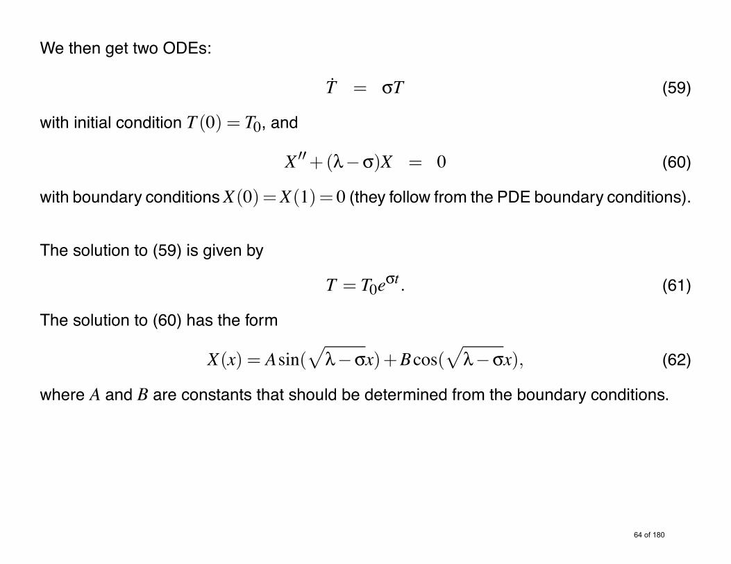
We then get two ODEs:

T = *T (59)

with initial condition T (0) = T0, and

X **+("&*)X = 0 (60)

with boundary conditionsX(0) =X(1)= 0 (they follow from the PDE boundary conditions).

The solution to (59) is given by

T = T0e*t. (61)

The solution to (60) has the form

X(x) = Asin(&

"&*x)+Bcos(&

"&*x), (62)

where A and B are constants that should be determined from the boundary conditions.

We have:

X(0) = 0, B= 0 ,

X(1) = 0, Asin(&

"&*) = 0 .

The last equality can only hold true if-"&* = )n for n= 0,1,2, . . ., so that

* = "&)2n2, n= 0,1,2, . . . (63)

Substituting (61), (62) into (56) yields

un(x, t) = T0Ane("&)2n2)t sin()nx), n= 0,1,2, . . . (64)

For linear PDEs the sum of particular solutions is also a solution (the principle of superpo-sition). Therefore the formal general solution of (53)–(55) is given by

u(x, t) =$+n=0

Cne("&)2n2)t sin()nx) (65)

whereCn = AnT0.

To determine the constants Cn, let us set t = 0 in (65) and multiply both sides of theresulting equality with sin()mx):

u0(x)sin()mx) = sin()mx)$+n=1

Cn sin()nx) . (66)

Then, using the identityZ 1

0sin()mx)sin()nx)dx=

'

1/2 n= m0 n .= m

(

(67)

we get

Cn =12

Z 1

0u0(x)sin()nx)dx . (68)

Substituting this expression into (65), we get

u(x, t) = 2$+n=1

e("&)2n2)t sin()nx)Z 1

0sin()nx)u0(x)dx (69)

Even though we obtained this solution formally, it can be proved that this is indeed a welldefined solution in a sense that it is unique, has continuous spatial derivatives up to asecond order, and depends continuously on the initial data.

Let us look at the structure of this solution. It consists of the following elements:

• eigenvalues (all real): "&)2n2, n= 1,2, . . .

• eigenfunctions: sin()nx)

• effect of initial conditions:R 10 sin()nx)u0(x)dx

The largest eigenvalue "&)2 (n= 1) indicates the rate of growth or decay of the solution.We can see that the plant is stable for "% )2 and is unstable otherwise.

After the transient response due to the initial conditions, the profile of the state will beproportional to the first eigenfunction sin()x), since other modes decay much faster.

Sometimes it is possible to use the method of separation of variables to determine thestability properties of the plant even though the complete closed form solution cannot beobtained.

Example 2 Let us find the values of the parameter g for which the system

ut = uxx+gu(0) (70)ux(0) = 0 (71)u(1) = 0 (72)

is unstable.

This example is motivated by the model of thermal instability in solid propellant rockets,where the term gu(0) is roughly the burning of the propellant at one end of the fuel cham-ber.

Using the method of separation of variables we set u(x, t) = X(x)T (t) and (70) gives:

T (t)T (t)

=X **(x)+gX(0)

X(x)= * . (73)

Hence, T (t) = T (0)e*t , whereas the solution of the ODE for X is given by

X(x) = Asinh(-*x)+Bcosh(

-*x)+

g*X(0) . (74)

Here the last term is a particular solution of a nonhomogeneous ODE (73).

Now we find the constant B in terms of X(0) by setting x = 0 in the above equation. Thisgives B= X(0)(1&g/*).

Using the boundary condition (71) we get A= 0 so that

X(x) = X(0))g*

+$

1&g*

%

cosh(-*x)

*

. (75)

Using the other boundary condition (72), we get the eigenvalue relationshipg*

=$g*&1

%

cosh(-*) . (76)

The above equation has no closed form solution. However, in this particular example wecan still find the stability region by finding values of g for which there are eigenvalues withzero real parts. First we check if * = 0 satisfies (76) for some values of g.

Using the Taylor expansion for cosh(-*), we get

g*

=$g*&1

%$

1+*2

+O(*2)%

=g*&1+

g2&*2

+O(*), (77)

which gives

g+ 2 as *+ 0

To show that there are no other eigenvalues on the imaginary axis, we set * = 2 jy2, y > 0. Equation (76)then becomes

cosh(( j+1)y) =g

g&2 jy2

cos(y)cosh(y)+ j sin(y)sinh(y) =g2+2 jgy2

g2+4y4.

Taking the absolute value, we get

sinh(y)2+ cos(y)2 =g4+4g2y4

(g2+4y4)2. (78)

The only solution to this equation is y= 0, which can be seen by computing derivatives of both sides of (78):

ddy

(sinh(y)2+ cos(y)2) = sinh(2y)& sin(2y) > 0 for all y> 0 (79)

ddy

g4+4g2y4

(g2+4y4)2= &

16g2y3

(g2+4y4)2< 0 for all y> 0 . (80)

Therefore, both sides of (78) start at the same point at y= 0 and for y > 0 the left hand side monotonicallygrows while the right hand side monotonically decays.

We thus proved that the plant (70)–(72) is neutrally stable only when g= 2.

SUMMARY: the plant is stable for g< 2 and unstable for g> 2.

Notes and References

The method of separation of variables is discussed in detail in classical PDE texts

R. COURANT AND D. HILBERT,Methods of mathematical physics, New York, IntersciencePublishers, 1962.

E. ZAUDERER, Partial differential equations of applied mathematics, New York : Wiley,2nd ed., 1998.

The exact solutions for many problems can be found in

H. S. CARSLAW AND J. C. JAEGER, Conduction of Heat in Solids, Oxford, ClarendonPress, 1959.

A. D. POLIANIN, Handbook of Linear Partial Differential Equations for Engineers andScientists, Boca Raton, Fla, Chapman and Hall/CRC, 2002.

Transform methods for PDEs are studied extensively in

D. G. DUFFY, Transform methods for solving partial differential equations, Boca Raton,FL : CRC Press, 1994.

Homework

1. Consider the Reaction-Diffusion equation

ut = uxx+"ufor x " (0,1) with the initial condition u0(x) = u(x,0) and boundary conditions

ux(0) = 0u(1) = 0 .

1) Find the solution of this PDE.

2) For what values of the parameter " is this system unstable?

2. Consider the heat equation

ut = uxxwith Robin’s boundary conditions

ux(0) = &qu(0)u(1) = 0 .

Find the range of values of the parameter q for which this system is unstable.

Backstepping for Parabolic PDEs

(Reaction-Advection-Diffusion and Other Equations)

The most important part of this course.

We introduce the method of backstepping, using the class of parabolic PDEs.

Later we extend backstepping to 1st and 2nd-order hyperbolic PDEs and to other classes.

Parabolic PDEs are first order in time and, while they can have a large number of unstableeigenvalues, this number is finite, which makes them more easily accessible to a readerwith background in ODEs.

Backstepping is capable of eliminating destabilizing forces/terms acting in the domain’sinterior, using control that acts only on the boundary.

We build a state transfornation, which involves a Volterra integral operator that ‘absorbs’the destabilizing terms acting in the domain and brings them to the boundary, where controlcan eliminate them.

The Volterra operator has a lower triangular structure.

ODE Backstepping

The backstepping method and its name originated in the early 1990’s for stabilization ofnonlinear ODE systems

M. KRSTIC, I. KANELLAKOPOULOS, AND P. KOKOTOVIC, Nonlinear and AdaptiveControl Design, Wiley, New York, 1995.

Consider the following three-state nonlinear system

y1 = y2+ y31 (81)y2 = y3+ y32 (82)y3 = u+ y33 (83)

Since the control input u is only in the last equation (83), we view it as boundary control.

The nonlinear terms y31, y32, y

33 can be viewed as nonlinear “reaction” terms. They are

destabilizing because, for u = 0, the overall system is a “cascade” of three unstable sub-systems of the form yi = y3i (the open-loop system exhibits a finite-time escape instability).

The control u can cancel the “matched” term y33 in (83) but cannot cancel directly theunmatched terms y31 and y32 in (81), (83).

To achieve the cancellation of all three of the destabilizing y3i -terms, a backstepping changeof variable is constructed recursively,

z1 = y1 (84)z2 = y2+ y31+ cy1 (85)z3 = y3+ y32+(3y21+2c)y2+3y51+2cy31+(c2+1)y1 , (86)

along with the control law

u = &c3z3& z2& y33& (3y22+3y21+2c)(y3+ y32)& (6y1y2+15y41+6cy21+ c2+1)(y2+ y31) , (87)

which convert the system (81)–(83) into

z1 = z2& cz1 (88)z2 = &z1+ z3& cz2 (89)z3 = &z2& cz3 , (90)

where the control parameter c should be chosen positive.

The system (88)–(90), which can also be written as

z= Az (91)

where

A=

+

,

&c 1 0&1 &c 10 &1 &c

-

. , (92)

is exponentially stable because

A+AT = &cI . (93)

The equality (93) guarantees that the Lyapunov function

V =12zT z (94)

has a negative definite time derivative

V = &czT z= &2cV . (95)

Hence, the target system (88)–(90) is desirable.

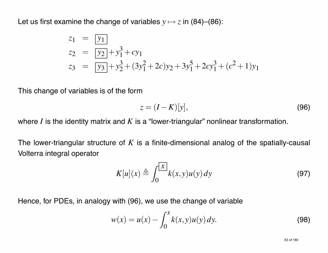
Let us first examine the change of variables y /+ z in (84)–(86):

z1 = y1z2 = y2 + y31+ cy1z3 = y3 + y32+(3y21+2c)y2+3y51+2cy31+(c2+1)y1

This change of variables is of the form

z= (I&K)[y], (96)

where I is the identity matrix and K is a “lower-triangular” nonlinear transformation.

The lower-triangular structure of K is a finite-dimensional analog of the spatially-causalVolterra integral operator

K[u](x) !

Z x

0k(x,y)u(y)dy (97)

Hence, for PDEs, in analogy with (96), we use the change of variable

w(x) = u(x)&Z x

0k(x,y)u(y)dy. (98)

An important feature of the change of variable

z1 = y1z2 = y2 + y31+ cy1z3 = y3 + y32+(3y21+2c)y2+3y51+2cy31+(c2+1)y1

is that it is invertible, i.e., y can be expressed as a smooth function of z (to be specific,

y1 = z1y2 = z2& z31& cz1y3 = z3& · · ·

In the PDE case, the transformation u /+ w in (98) is also invertible and the inverse can bewritten as

u(x) = w(x)+Z x

0l(x,y)w(y)dy. (99)

Next, let us examine the relation between the target systems

z= Az , A=

+

,

&c 1 0&1 &c 10 &1 &c

-

. (100)

and the heat equation as a target system for parabolic PDEs,

wt = wxx . (101)

They both admit a simple 2-norm as a Lyapunov function, specifically,

ddt12zT z= &czT z (102)

in the ODE case andddt12

Z 1

0w(x)2dx= &

Z 1

0wx(x)2dx (103)

in the PDE case.

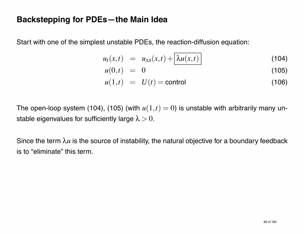
Backstepping for PDEs—the Main Idea

Start with one of the simplest unstable PDEs, the reaction-diffusion equation:

ut(x, t) = uxx(x, t)+ "u(x, t) (104)u(0, t) = 0 (105)u(1, t) = U(t) = control (106)

The open-loop system (104), (105) (with u(1, t) = 0) is unstable with arbitrarily many un-stable eigenvalues for sufficiently large " > 0.

Since the term "u is the source of instability, the natural objective for a boundary feedbackis to “eliminate” this term.

State transformation

w(x, t) = u(x, t)&Z x

0k(x,y)u(y, t)dy (107)

Feedback control

u(1, t) =Z 1

0k(1,y)u(y, t)dy (108)

Target system (exp. stable)

wt(x, t) = wxx(x, t) (109)w(0, t) = 0 (110)w(1, t) = 0 (111)

Task: find kernel k(x,y).

The Volterra integral transformation in (107) has the following features:

The limits of integral are from 0 to x, not from 0 to 1.

“Spatially causal,” that is, for a given x the right hand side of (107) depends onlyon the values of u in the interval [0,x].

Invertible because of the presence of the identity operator and the spatial causal-ity of the Volterra operator. Because of invertibility, stability of the target systemtranslates into stability of the closed loop system consisting of the plant plusboundary feedback.

Gain Kernel PDE

Task: find the function k(x,y) (which we call “gain kernel”) that makes the plant (104), (105)with the controller (108) equivalent to the target system (109)–(111).

We introduce the following notation:

kx(x,x) =!!xk(x,y)|y=x

ky(x,x) =!!yk(x,y)|y=x

ddxk(x,x) = kx(x,x)+ ky(x,x).

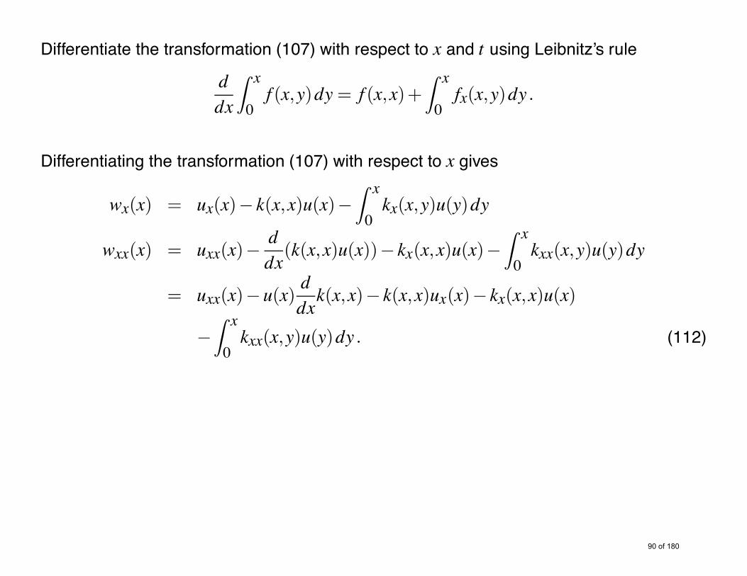
Differentiate the transformation (107) with respect to x and t using Leibnitz’s rule

ddx

Z x

0f (x,y)dy= f (x,x)+

Z x

0fx(x,y)dy .

Differentiating the transformation (107) with respect to x gives

wx(x) = ux(x)& k(x,x)u(x)&Z x

0kx(x,y)u(y)dy

wxx(x) = uxx(x)&ddx

(k(x,x)u(x))& kx(x,x)u(x)&Z x

0kxx(x,y)u(y)dy

= uxx(x)&u(x)ddxk(x,x)& k(x,x)ux(x)& kx(x,x)u(x)

&Z x

0kxx(x,y)u(y)dy . (112)

Next, we differentiate the transformation (107) with respect to time:

wt(x) = ut(x)&Z x

0k(x,y)ut(y)dy

= uxx(x)+"u(x)&Z x

0k(x,y)

/

uyy(y)+"u(y)0

dy

= uxx(x)+"u(x)& k(x,x)ux(x)+ k(x,0)ux(0)

+Z x

0ky(x,y)uy(y)dy&

Z x

0"k(x,y)u(y)dy (integration by parts)

= uxx(x)+"u(x)& k(x,x)ux(x)+ k(x,0)ux(0)+ ky(x,x)u(x)& ky(x,0)u(0)

&Z x

0kyy(x,y)u(y)dy&

Z x

0"k(x,y)u(y)dy . (integration by parts) (113)

Subtracting (112) from (113), we get

wt&wxx =

1

"+2ddxk(x,x)

2

u(x)+ k(x,0)ux(0)

+Z x

0

/

kxx(x,y)& kyy(x,y)&"k(x,y)0

u(y)dy

= 0

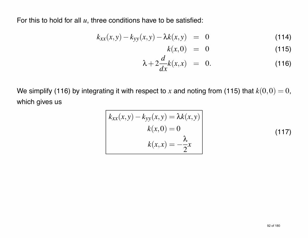
For this to hold for all u, three conditions have to be satisfied:

kxx(x,y)& kyy(x,y)&"k(x,y) = 0 (114)k(x,0) = 0 (115)

"+2ddxk(x,x) = 0. (116)

We simplify (116) by integrating it with respect to x and noting from (115) that k(0,0) = 0,which gives us

kxx(x,y)& kyy(x,y) = "k(x,y)k(x,0) = 0

k(x,x) = &"2x

(117)

These three conditions form a well posed PDE of hyperbolic type in the “Goursat form.”

One can think of the k-PDE as a wave equation with an extra term "k.

x plays the role of time and y of space.

In quantum physics such PDEs are called Klein-Gordon PDEs.

Domain of the PDE for gain kernel k(x,y).

The boundary conditions are prescribed on hypotenuse and the lower cathetus of thetriangle.

The value of k(x,y) on the vertical cathetus gives us the control gain k(1,y).

Converting Gain Kernel PDE to an Integral Equation

To find a solution of the k-PDE (117) we first convert it into an integral equation.

Introducing the change of variables

% = x+ y, , = x& y (118)

we have

k(x,y) = G(%,,)

kx = G%+G,

kxx = G%%+2G%,+G,,

ky = G%&G,

kyy = G%%&2G%,+G,, .

Thus, the gain kernel PDE becomes

G%,(%,,) ="4G(%,,) (119)

G(%,%) = 0 (120)

G(%,0) = &"4% . (121)

Integrating (119) with respect to , from 0 to ,, we get

G%(%,,) = G%(%,0)+Z ,

0

"4G(%,s)ds = &

"4

+Z ,

0

"4G(%,s)ds . (122)

Next, we integrate (122) with respect to % from , to % to get the integral equation

G(%,,) = &"4(%&,)+

"4

Z %

,

Z ,

0G(&,s)dsd& (123)

The G-integral eqn is easier to analyze than the k-PDE.

Method of Successive Approximations

Start with an initial guess

G0(%,,) = 0 (124)

and set up the recursive formula for (123) as follows:

Gn+1(%,,) = &"4(%&,)+

"4

Z %

,

Z ,

0Gn(&,s)dsd& (125)

If this functional iteration converges, we can write the solution G(%,,) as

G(%,,) = limn+$

Gn(%,,) . (126)

Let us denote the difference between two consecutive terms as

-Gn(%,,) = Gn+1(%,,)&Gn(%,,) . (127)

Then

-Gn+1(%,,) ="4

Z %

,

Z ,

0-Gn(&,s)dsd& (128)

and (126) can be alternatively written as

G(%,,) =$+n=0

-Gn(%,,) . (129)

Computing -Gn from (128) starting with

-G0 = G1(%,,) = &"4(%&,) , (130)

we can observe the pattern which leads to the following formula:

-Gn(%,,) = &(%&,)%n,n

n!(n+1)!

!"4

"n+1(131)

This formula can be verified by induction.

The solution to the integral equation is given by

G(%,,) = &$+n=0

(%&,)%n,n

n!(n+1)!

!"4

"n+1. (132)

To compute the series (132), note that a first order modified Bessel function of the first kindcan be represented as

I1(x) =$+n=0

(x/2)2n+1

n!(n+1)!. (133)

ASIDE: Modified Bessel Functions InThe function y(x) = In(x) is a solution to the following ODE

x2y**+ xy* & (x2+n2)y= 0 (134)

Series representation

In(x) =$+m=0

(x/2)n+2m

m!(m+n)!(135)

Properties

2nIn(x) = x(In&1(x)& In+1(x)) (136)

In(&x) = (&1)nIn(x) (137)

DifferentiationddxIn(x) =

12(In&1(x)+ In+1(x)) =

nxIn(x)+ In+1(x) (138)

ddx

(xnIn(x)) = xnIn&1,ddx

(x&nIn(x)) = x&nIn+1 (139)

Asymptotic properties

In(x) 01n!

$x2

%n, x+ 0 (140)

In(x) 0ex-2)x

, x+ $ (141)

0 1 2 3 4 5

0

2

4

6

8

10I0 I1 I2 I3

x

Modified Bessel functions In.

Comparing (135) with (132) we obtain

G(%,,) = &"2(%&,)

I1(&

"%,)&

"%,(142)

or, returning to the original x, y variables,

k(x,y) = &"yI1

!3

"(x2& y2)"

3

"(x2& y2)(143)

k1(y)

y

! = 10

! = 15

! = 20

! = 25

0 0.2 0.4 0.6 0.8 1-40

-30

-20

-10

0

Control gain k(1,y) for different values of "

As " gets larger, the plant becomes more unstable which requires more control effort.

Low gain near the boundaries is logical: near x= 0 the state is small even without controlbecause of the boundary condition u(0) = 0; near x= 1 the control has the most impact.

Inverse Transformation

We need to establish that stability of the w-target system (109)–(111) impliesstability of the u-closed-loop system (104), (105), (108), by showing that thetransformation u /+ w is invertible.

Postulate an inverse transformation in the form

u(x) = w(x)+Z x

0l(x,y)w(y)dy , (144)

where l(x,y) is the transformation kernel.

Given the direct transformation (107) and the inverse transformation (144), the kernelsk(x,y) and l(x,y) satisfy

l(x,y) = k(x,y)+Z x

yk(x,%)l(%,y)d% (145)

Proof of (145). First recall from calculus the following formula for changing the order ofintegration:

Z x

0

Z y

0f (x,y,%)d%dy=

Z x

0

Z x

%f (x,y,%)dyd% (146)

Substituting (144) into (107), we get

w(x) = w(x)+Z x

0l(x,y)w(y)dy&

Z x

0k(x,y)

1

w(y)+Z y

0l(y,%)w(%)d%

2

dy

= w(x)+Z x

0l(x,y)w(y)dy&

Z x

0k(x,y)w(y)dy&

Z x

0

Z y

0k(x,y)l(y,%)w(%)d%dy

0 =Z x

0w(y)

1

l(x,y)& k(x,y)&Z x

yk(x,%)l(%,y)d%

2

dy .

Since the last line has to hold for all w(y), we get the relationship (145). "

The formula (145) is general (it does not depend on the plant and the target system) but isnot very helpful in actually finding l(x,y) from k(x,y).

Instead, we follow the same approach that led us to the kernel PDE for k(x,y).

Differentiating (144) with respect to time we get

ut(x) = wt(x)+Z x

0l(x,y)wt(y)dy

= wxx(x)+ l(x,x)wx(x)& l(x,0)wx(0)& ly(x,x)w(x)

+Z x

0lyy(x,y)w(y)dy (147)

and differentiating twice with respect to x gives

uxx(x) = wxx(x)+ lx(x,x)w(x)+w(x)ddxl(x,x)+ l(x,x)wx(x)

+Z x

0lxx(x,y)w(y)dy . (148)

Subtracting (148) from (147) we get

"w(x)+"Z x

0l(x,y)w(y)dy = &2w(x)

ddxl(x,x)& l(x,0)wx(0)

+Z x

0(lyy(x,y)& lxx(x,y))w(y)dy

which gives the following conditions on l(x,y):

lxx(x,y)& lyy(x,y) = &"l(x,y)l(x,0) = 0

l(x,x) = &"2x

(149)

Comparing this PDE with the PDE (117) for k(x,y), we see that

l(x,y;") = &k(x,y;&") . (150)

From (143) we have

l(x,y) = &"yI1

!3

&"(x2& y2)"

3

&"(x2& y2)= &"y

I1!

j3

"(x2& y2)"

j3

"(x2& y2),

or, using the properties of I1,

l(x,y) = &"yJ1

!3

"(x2& y2)"

3

"(x2& y2)(151)

ASIDE: Bessel Functions JnThe function y(x) = Jn(x) is a solution to the following ODE

x2y**+ xy*+(x2&n2)y= 0 (152)

Series representation

Jn(x) =$+m=0

(&1)m(x/2)n+2m

m!(m+n)!(153)

Relationship with Jn(x)

In(x) = i&nJn(ix), In(ix) = inJn(x) (154)

Properties

2nJn(x) = x(Jn&1(x)+ Jn+1(x)) (155)

Jn(&x) = (&1)nJn(x) (156)

DifferentiationddxJn(x) =

12(Jn&1(x)& Jn+1(x)) =

nxJn(x)& Jn+1(x) (157)

ddx

(xnJn(x)) = xnJn&1,ddx

(x&nJn(x)) = &x&nJn+1 (158)

Asymptotic properties

Jn(x) 01n!

$x2

%n, x+ 0 (159)

Jn(x) 04

2)xcos

$

x&)n2&)4

%

, x+ $ (160)

0 2 4 6 8 10!0.5

0

0.5

1

J1

J0

J3J2

x

Bessel functions Jn.

Summary of control design for the reaction-diffusion equation

Plant ut = uxx+"u (161)u(0) = 0 (162)

Controller u(1) = &Z 1

0y"I1

!3

"(1& y2)"

3

"(1& y2)u(y)dy (163)

Transformation w(x) = u(x)+Z x

0"yI1

!3

"(x2& y2)"

3

"(x2& y2)u(y)dy (164)

u(x) = w(x)&Z x

0"yJ1

!3

"(x2& y2)"

3

"(x2& y2)w(y)dy (165)

Target system wt = wxx (166)w(0) = 0 (167)w(1) = 0 (168)

0

0.5

1 00.05

0.10

10

20

30

40

tx

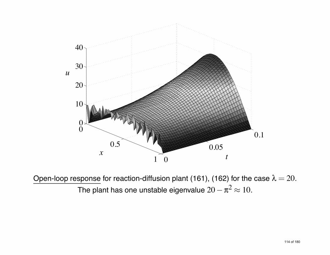
u

Open-loop response for reaction-diffusion plant (161), (162) for the case " = 20.The plant has one unstable eigenvalue 20&)2 0 10.

00.5

1 0 0.1 0.2 0.3 0.4 0.5

!40

!30

!20

!10

0

10

20

tx

u

Closed-loop response with controller (163) implemented.

0 0.1 0.2 0.3 0.4 0.5!40

!30

!20

!10

0

10

t

u(1, t)

The control (163) for reaction-diffusion plant (161)–(162).

Example 3 Consider the plant with a Neumann boundary cond. on the uncontrolled end,

ut = uxx+"u (169)ux(0) = 0 (170)u(1) = U(t) . (171)

We use the transformation

w(x) = u(x)&Z x

0k(x,y)u(y)dy (172)

to map this plant into the target system

wt = wxx (173)wx(0) = 0 (174)w(1) = 0 . (175)

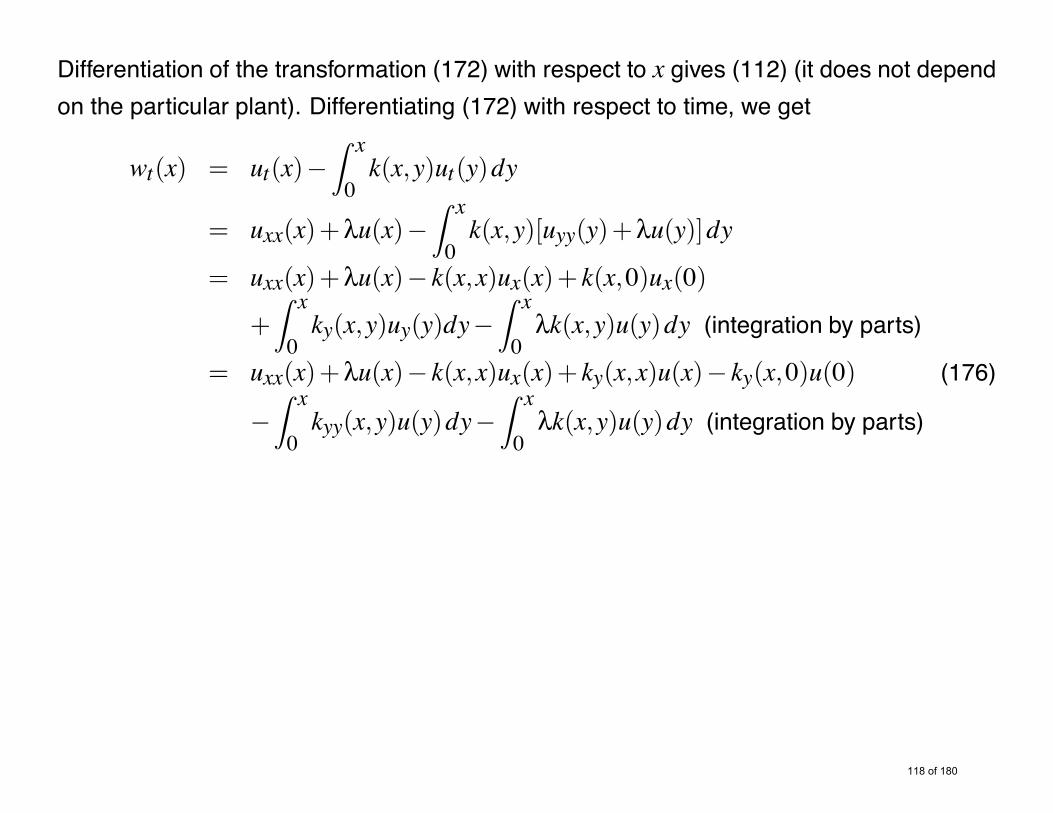
Differentiation of the transformation (172) with respect to x gives (112) (it does not dependon the particular plant). Differentiating (172) with respect to time, we get

wt(x) = ut(x)&Z x

0k(x,y)ut(y)dy

= uxx(x)+"u(x)&Z x

0k(x,y)[uyy(y)+"u(y)]dy

= uxx(x)+"u(x)& k(x,x)ux(x)+ k(x,0)ux(0)

+Z x

0ky(x,y)uy(y)dy&

Z x

0"k(x,y)u(y)dy (integration by parts)

= uxx(x)+"u(x)& k(x,x)ux(x)+ ky(x,x)u(x)& ky(x,0)u(0) (176)

&Z x

0kyy(x,y)u(y)dy&

Z x

0"k(x,y)u(y)dy (integration by parts)

Subtracting (112) from (176), we get

wt&wxx =

1

"+2ddxk(x,x)

2

u(x)& ky(x,0)u(0)

+Z x

0

/

kxx(x,y)& kyy(x,y)&"k(x,y)0

u(y)dy . (177)

For the right hand side of this equation to be zero for all u(x), three conditions must besatisfied:

kxx(x,y)& kyy(x,y)&"k(x,y) = 0 (178)ky(x,0) = 0 (179)

"+2ddxk(x,x) = 0 . (180)

Integrating (180) with respect to x gives k(x,x) = &"/2x+ k(0,0), where k(0,0) is ob-tained using the boundary condition (174):

wx(0) = ux(0)+ k(0,0)u(0) = 0 ,

so that k(0,0) = 0. The gain kernel PDE is thus

kxx(x,y)& kyy(x,y) = "k(x,y) (181)ky(x,0) = 0 (182)

k(x,x) = &"2x . (183)

Note that this PDE is very similar to (117). The only difference is in the boundary condi-tion at y = 0. The solution to the PDE (181)–(183) is obtained through a summation ofsuccessive approximation series, similarly to the way it was obtained for the PDE (117):

k(x,y) = &" x1I1

!3

"(x2& y2)"

3

"(x2& y2)(184)

Thus, the controller is given by

u(1) = &Z 1

0"I1

!3

"(1& y2)"

3

"(1& y2)u(y)dy . (185)

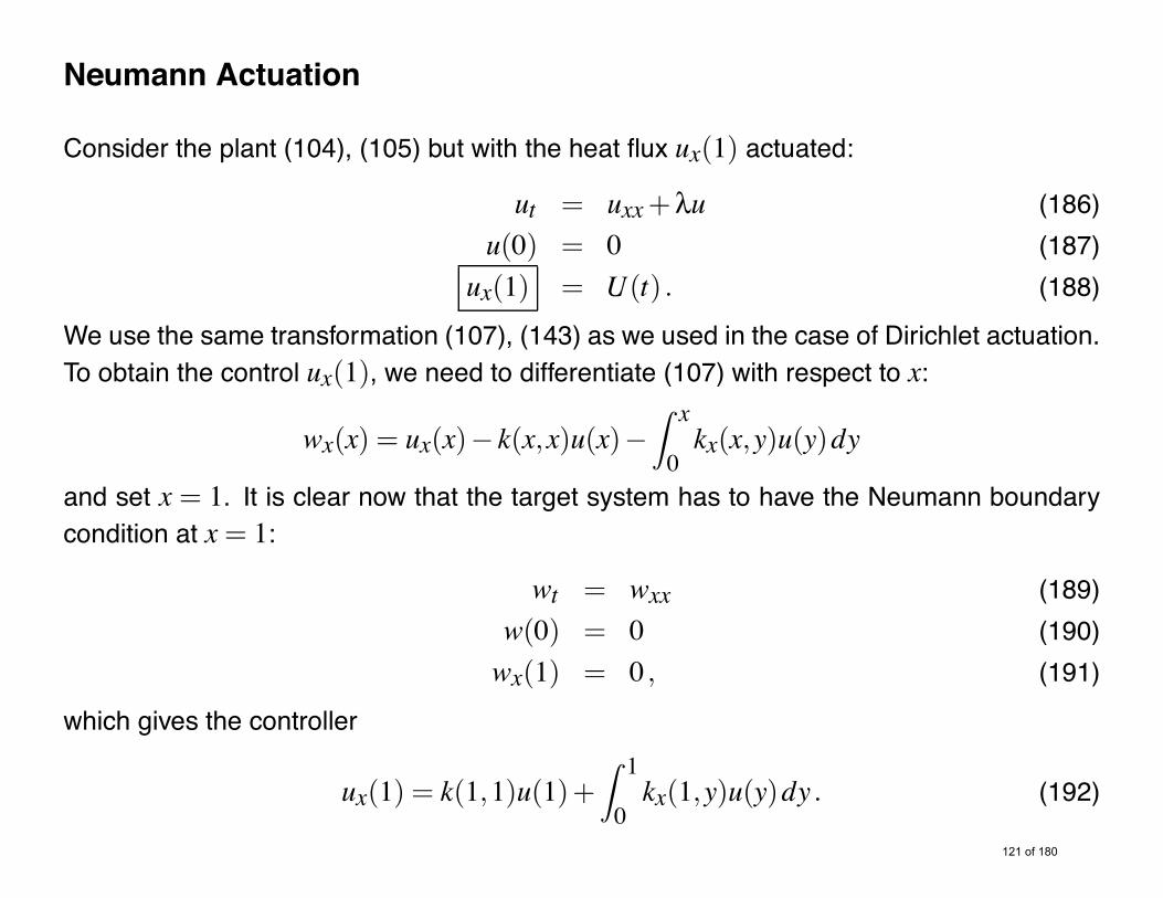
Neumann Actuation

Consider the plant (104), (105) but with the heat flux ux(1) actuated:

ut = uxx+"u (186)u(0) = 0 (187)

ux(1) = U(t) . (188)

We use the same transformation (107), (143) as we used in the case of Dirichlet actuation.To obtain the control ux(1), we need to differentiate (107) with respect to x:

wx(x) = ux(x)& k(x,x)u(x)&Z x

0kx(x,y)u(y)dy

and set x = 1. It is clear now that the target system has to have the Neumann boundarycondition at x= 1:

wt = wxx (189)w(0) = 0 (190)wx(1) = 0 , (191)

which gives the controller

ux(1) = k(1,1)u(1)+Z 1

0kx(1,y)u(y)dy . (192)

All that remains is to derive the expression for kx from (143) using the properties of Besselfunctions:

kx(x,y) = &"yxI2

!3

"(x2& y2)"

x2& y2.

Finally, the controller is

ux(1) = &"2u(1)&

Z 1

0"yI2

!3

"(1& y2)"

1& y2u(y)dy. (193)

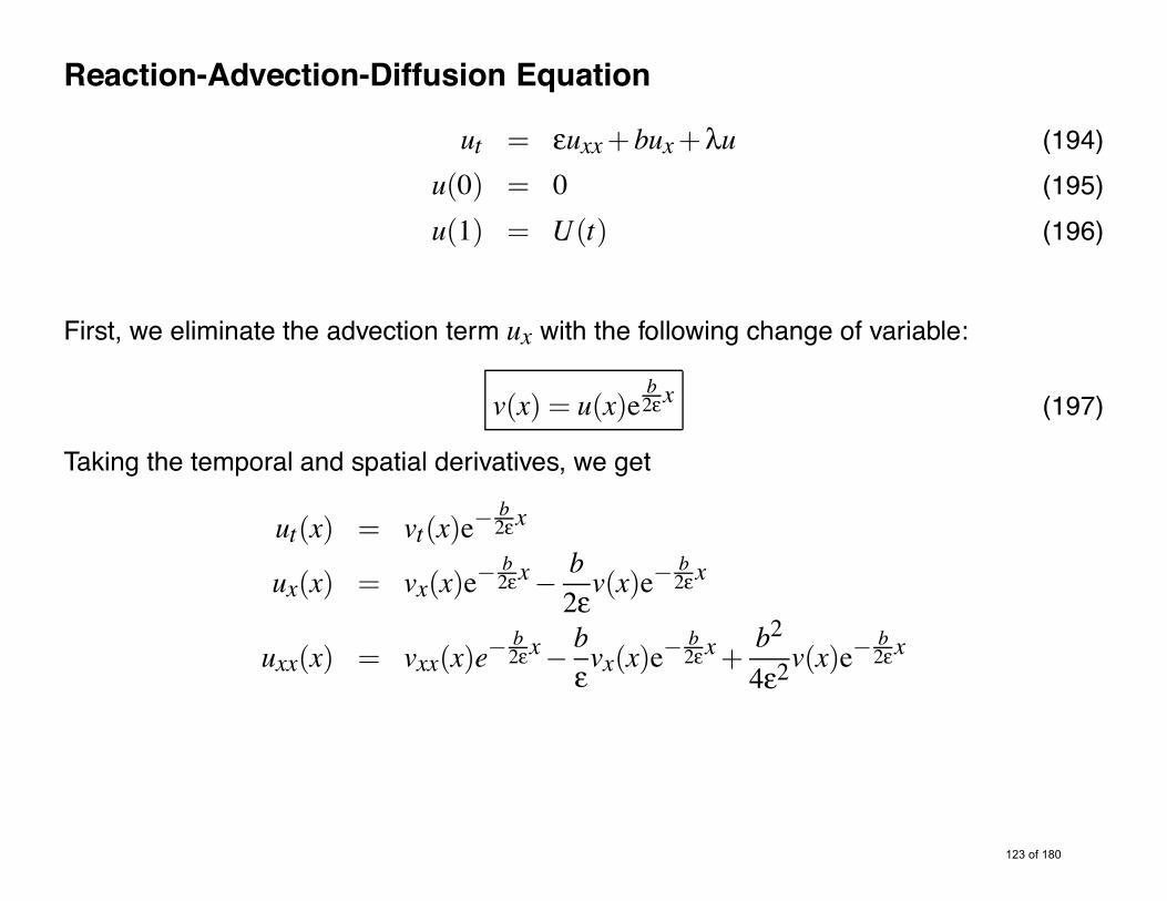
Reaction-Advection-Diffusion Equation

ut = 'uxx+bux+"u (194)u(0) = 0 (195)u(1) = U(t) (196)

First, we eliminate the advection term ux with the following change of variable:

v(x) = u(x)eb2'x (197)

Taking the temporal and spatial derivatives, we get

ut(x) = vt(x)e&b2'x

ux(x) = vx(x)e&b2'x&

b2'v(x)e&

b2'x

uxx(x) = vxx(x)e&b2'x&

b'vx(x)e&

b2'x+

b2

4'2v(x)e&

b2'x

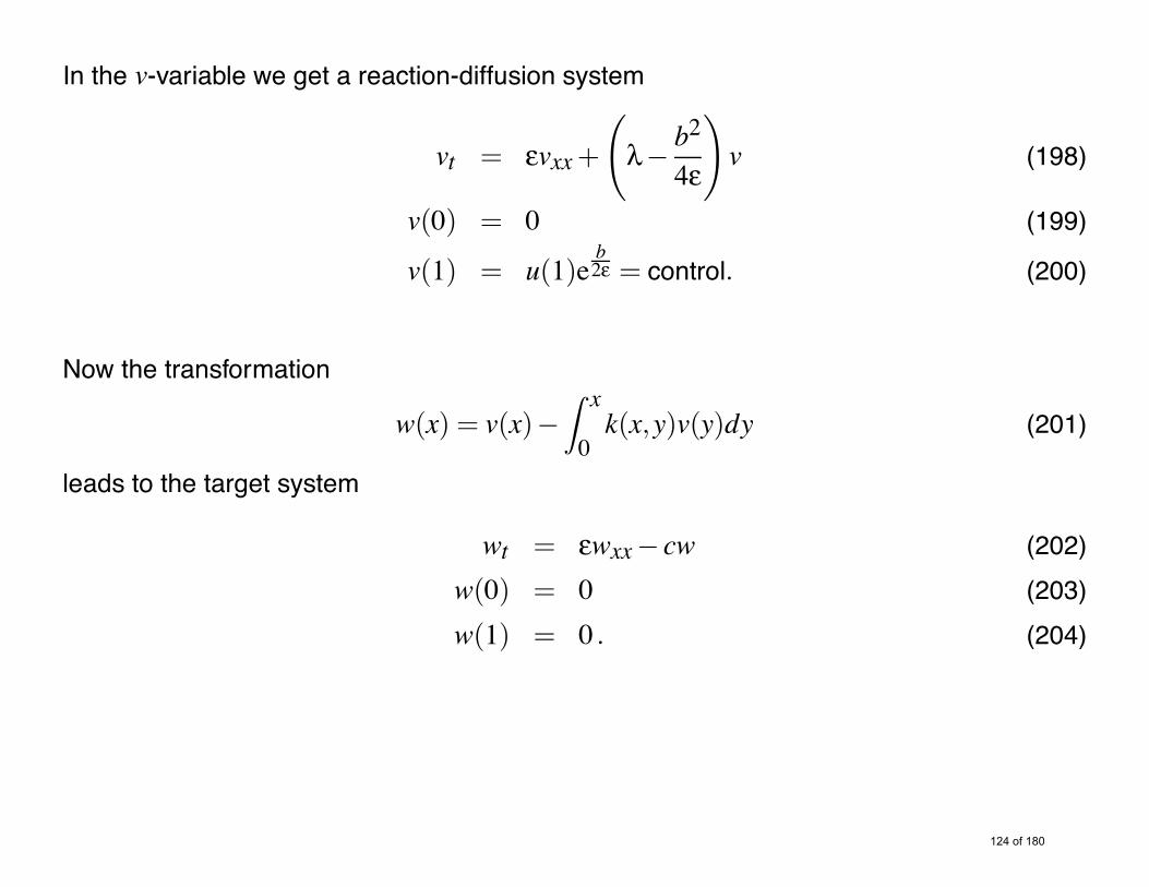
In the v-variable we get a reaction-diffusion system

vt = 'vxx+

5

"&b2

4'

6

v (198)

v(0) = 0 (199)

v(1) = u(1)eb2' = control. (200)

Now the transformation

w(x) = v(x)&Z x

0k(x,y)v(y)dy (201)

leads to the target system

wt = 'wxx& cw (202)w(0) = 0 (203)w(1) = 0 . (204)

Here the constant c is a design parameter that sets the decay rate of the closed loopsystem. It should satisfy the following stability condition:

c'max

7

b2

4'&",0

8

.

The max is used to prevent spending unnecessary control effort when the plant is stable.

The gain kernel k(x,y) can be shown to satisfy the following PDE:

'kxx(x,y)& 'kyy(x,y) =

5

"&b2

4'+ c

6

k(x,y) (205)

k(x,0) = 0 (206)

k(x,x) = &x2'

5

"&b2

4'+ c

6

. (207)

This equation is exactly the same as (117), just with a different constant instead of ",

"0 =1'

5

"&b2

4'+ c

6

. (208)

Therefore the solution to (205)–(207) is given by

k(x,y) = &"0yI1

!3

"0(x2& y2)"

3

"0(x2& y2). (209)

The controller is

u(1) =Z 1

0e&

b2'(1&y)"0y

I1!3

"0(1& y2)"

3

"0(1& y2)u(y)dy . (210)

Let us examine the effect of the advection term bux in (194) on open-loop stability and onthe size of the control gain. From (198) we see that the advection term has a beneficialeffect on open-loop stability, irrespective of the sign of the advection coefficient b. However,the effect of b on the gain function in the control law in (210) is ‘sign-sensitive.’ Negativevalues of b demand much higher control effort than positive values of b. Interestingly,negative values of b refer to the situation where the state disturbances advect towards theactuator at x= 1, whereas the ‘easier’ case of positive b refers to the case where the statedisturbances advect away from the actuator at x = 1 and towards the Dirichlet boundarycondition (195) at x= 0.

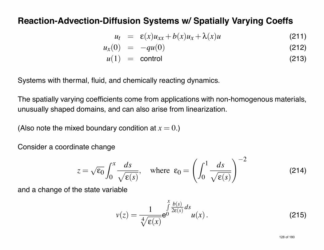
Reaction-Advection-Diffusion Systems w/ Spatially Varying Coeffsut = '(x)uxx+b(x)ux+"(x)u (211)

ux(0) = &qu(0) (212)u(1) = control (213)

Systems with thermal, fluid, and chemically reacting dynamics.

The spatially varying coefficients come from applications with non-homogenous materials,unusually shaped domains, and can also arise from linearization.

(Also note the mixed boundary condition at x= 0.)

Consider a coordinate change

z=-'0

Z x

0

ds&

'(s), where '0 =

5Z 1

0

ds&

'(s)

6&2

(214)

and a change of the state variable

v(z) =1

4&

'(x)e

xR

0

b(s)2'(s) dsu(x) . (215)

Then v satisfies the PDE:

vt(z, t) = '0vzz(z, t)+"0(z)v(z, t) (216)vz(0, t) = &q0v(0, t), (217)

where

'0 =

5Z 1

0

ds&

'(s)

6&2

(218)

"0(z) = "(x)+'**(x)4

&b*(x)2

&316

('*(x))2

'(x)+12b(x)'*(x)'(x)

&14b2(x)'(x)

(219)

q0 = q

#

'(0)'0

&b(0)

2&

'0'(0)&

'*(0)4&

'0'(0). (220)

We use the transformation (107) to map the modified plant into the target system

wt = '0wzz& cw (221)wz(0) = 0 (222)w(1) = 0 . (223)

The transformation kernel is found by solving the PDE

kzz(z,y)& kyy(z,y) ="0(y)+ c

'0k(z,y) (224)

ky(z,0) = &q0k(z,0) (225)

k(z,z) = &q0&12'0

Z z

0("0(y)+ c)dy . (226)

Well posed but cannot be solved in closed form. One can solve it either symbolically, usingthe successive approximation series, or numerically with finite difference schemes.

Since the controller for v-system is given by

v(1) =Z 1

0k(1,y)v(y)dy , (227)

using (214) and (215) we obtain the controller for the original u-plant:

u(1) =Z 1

0

'1/4(1)-'0'3/4(y)

e&1R

yb(s)2'(s) ds

k!

Z 1

0

4'0'(s)

ds,Z y

0

4'0'(s)

ds"

u(y)dy . (228)

'(x) k(1,y)

x

t

y

$u(·, t)$

0 0.1 0.2 0.3 0.4

0 0.5 10 0.5 1

0

1

2

3

4

5

-15

-10

-5

0

0

0.5

1

1.5

2

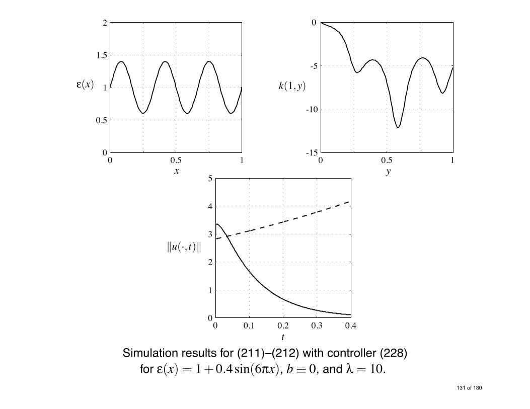
Simulation results for (211)–(212) with controller (228)for '(x) = 1+0.4sin(6)x), b2 0, and " = 10.

Other Spatially Causal Plants

ut = uxx+g(x)u(0)+Z x

0f (x,y)u(y)dy (229)

ux(0) = 0 , (230)

where u(1) is actuated.

Equation partly motivated by the model of unstable burning in solid propellant rockets

D. M. BOSKOVIC AND M. KRSTIC, Stabilization of a solid propellant rocket in-stability by state feedback, Int. J. of Robust and Nonlinear Control, vol. 13,pp. 483–495, 2003.

and the thermal convection loop

R. VAZQUEZ AND M. KRSTIC, Explicit integral operator feedback for local stabi-lization of nonlinear thermal convection loop PDEs, Systems and Control Letters,vol. 55, pp. 624–632, 2006.

PDE for the gain kernel:

kxx& kyy = & f (x,y)+Z x

yk(x,%) f (%,y)d% (231)

ky(x,0) = g(x)&Z x

0k(x,y)g(y)dy (232)

k(x,x) = 0 . (233)

Consider one case where explicitly solvable. Let f 2 0, then (231) becomes

kxx& kyy = 0 , (234)

which has a general solution of the form

k(x,y) = .(x& y)+/(x+ y). (235)

From the boundary condition (233) we get

.(0)+/(2x) = 0 , (236)

which means that, without a loss of generality, we can set /2 0 and .(0) = 0.

Therefore,

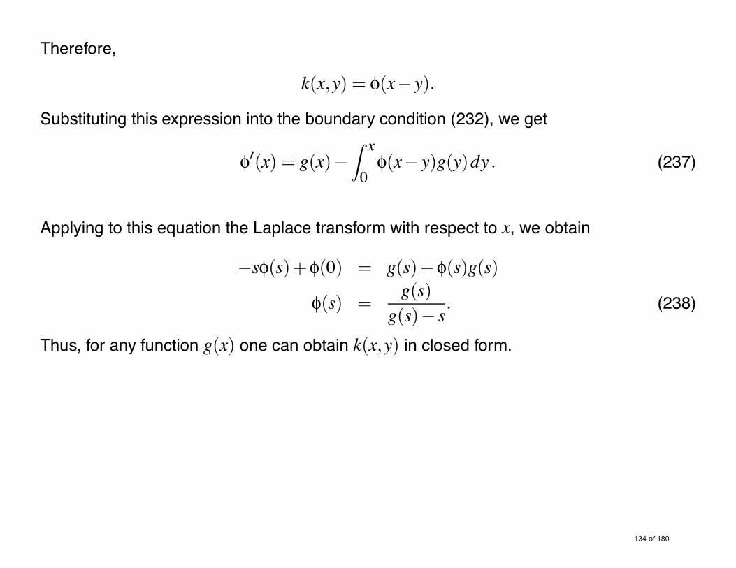
k(x,y) = .(x& y).

Substituting this expression into the boundary condition (232), we get

.*(x) = g(x)&Z x

0.(x& y)g(y)dy . (237)

Applying to this equation the Laplace transform with respect to x, we obtain

&s.(s)+.(0) = g(s)&.(s)g(s)

.(s) =g(s)

g(s)& s. (238)

Thus, for any function g(x) one can obtain k(x,y) in closed form.

Example 4 Let

g(x) = g.

Then

g(s) =gs.

and from (238), .(s) becomes

.(s) =g

g& s2= &

-g

-gs2&g

.

This gives

.(z) = &-gsinh(

-gz)

and

k(x,y) = &-gsinh(-g(x& y)).

Therefore, for the plant

ut = uxx+gu(0)ux(0) = 0

the stabilizing controller is given by

u(1) = &Z 1

0

-gsinh(-g(1& y))u(y)dy .

Comparison with ODE Backstepping

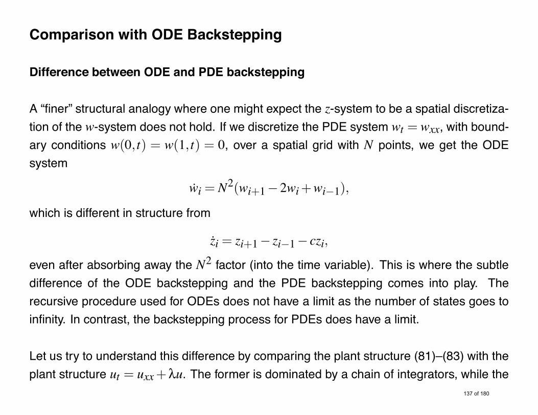
Difference between ODE and PDE backstepping

A “finer” structural analogy where one might expect the z-system to be a spatial discretiza-tion of the w-system does not hold. If we discretize the PDE system wt = wxx, with bound-ary conditions w(0, t) = w(1, t) = 0, over a spatial grid with N points, we get the ODEsystem

wi = N2(wi+1&2wi+wi&1),

which is different in structure from

zi = zi+1& zi&1& czi,

even after absorbing away the N2 factor (into the time variable). This is where the subtledifference of the ODE backstepping and the PDE backstepping comes into play. Therecursive procedure used for ODEs does not have a limit as the number of states goes toinfinity. In contrast, the backstepping process for PDEs does have a limit.

Let us try to understand this difference by comparing the plant structure (81)–(83) with theplant structure ut = uxx+"u. The former is dominated by a chain of integrators, while the

latter is dominated by the diffusion operator. While the diffusion operator is a well-defined,meaningful object, an “infinite integrator chain” is not. It is for this reason that the infinite-dimensional backstepping design succeeds only if particular care is taken to convert theunstable parabolic PDE ut = uxx+"u into a stable target system wt = wxx which is withinthe same PDE class, namely, parabolic.

To put it in simpler words, we make sure to retain the !xx term in the target system, eventhough it may be tempting to go for some other target system, such as, for example, thefirst-order hyperbolic (transport equation-like) PDE wt = wx& cw, which is more reminis-cent of the ODE target system (88)-(90). If such an attempt is made, the derivation of thePDE conditions for the kernel k(x,y) would not be successful and the matching of termsbetween the plant ut = uxx+"u and the target system wt =wxx&cw would result in termsthat cannot be cancelled.

Meaning of the term backstepping

In the ODE setting this procedure is referred to as integrator backstepping because, asillustrated with the help of example (81)-(83), the design procedure propagates the feed-back law synthesis “backwards” through a chain of integrators. Upon a careful inspectionof the change of variables (84)–(86), the first “step” of the backstepping procedure is totreat the state y2 as the control input in the subsystem y1 = y2+ y31, design the “controllaw” y2 = &y31& cy1, then “step back” through the integrator in the second subsystemy2 = y3+ y32 and design the “control” y3 so that the error state z2 = y2& (&y31& cy1)is forced to go zero, thus ensuring that the state y2 acts (approximately) as the controly2 =&y31&cy1. This “backward stepping” through integrators continues until one encoun-ters the actual control u in (87), which in the example (81)–(83) happens after two steps ofbackstepping.

Even though in our continuum version of backstepping for PDEs there are no simple inte-grators to step through, the analogy with the method for ODEs is in the triangularity of thechange of variable and the pursuit of a stable target system. For this reason, we retain theterm backstepping for PDEs.

Lower-triangular (strict-feedback) systems

Backstepping for ODEs is applicable to a fairly broad class of ODE systems which arereferred to as strict-feedback systems. These systems are characterized by having a chainof integrators, the control appearing in the last equation, and additional terms (linear ornonlinear) having a “lower-triangular” structure. In this lower-triangular structure the firstequation depends only on the first state, the term in the second equation depends on thefirst and the second states, and so on. In the example (81)–(83) the cubic terms had a“diagonal” dependence on the states yi and thus, their structure was lower triangular andhence the plant (81)–(83) was of strict-feedback type. The change of variables (84)–(86)has a general lower triangular form.

The capability of backstepping to deal with lower-triangular ODE structures has motivatedour extension of PDE backstepping from reaction-diffusion systems (which are of a “di-agonal” kind) to the systems with lower-triangular strict-feedback terms g(x)u(0, t) andR x0 f (x,y)u(y, t)dy. Such terms, besides being tractable by the backstepping method,

happen to be essential in several applications, including flexible beams and Navier-Stokesequations.

Notes and References

The backstepping idea for PDEs appeared well before the development of finite-dimensional backstepping in the late 1980s.

Volterra operator transformations used for solving PDEs in

D. COLTON, The solution of initial-boundary value problems for parabolic equa-tions by the method of integral operators, Journal of Differential Equations, 26(1977), pp. 181–190.

and for developing controllability results in

T. I. SEIDMAN, Two results on exact boundary control of parabolic equations,Applied Mathematics and Optimization, 11 (1984), pp. 145–152.

Homework

1. For the plant

ut = uxx+"uux(0) = 0

design the Neumann stabilizing controller (ux(1) actuated).

Hint: use the target system

wt = wxxwx(0) = 0

wx(1) = &12w(1) . (239)

This system is asymptotically stable. Note also that you do not need to find k(x,y),it has already been found in Example 3. You only need to use the condition (239) toderive the controller.

2. Find the PDE for the kernel l(x,y) of the inverse transformation

u(x) = w(x)+Z x

0l(x,y)w(y)dy ,

which relates the systems u and w from Exercise 1. By comparison with the PDE fork(x,y), show that

l(x,y) = &"xJ1

!3

"(x2& y2)"

3

"(x2& y2).

3. Design the Dirichlet boundary controller for the heat equation

ut = uxxux(0) = &qu(0)

Follow these steps:

1) Use the transformation

w(x) = u(x)&Z x

0k(x,y)u(y)dy (240)

to map the plant into the target system

wt = wxx (241)wx(0) = 0 (242)w(1) = 0 . (243)

Show that k(x,y) satisfies the following PDE:

kxx(x,y) = kyy(x,y) (244)ky(x,0) = &qk(x,0) (245)k(x,x) = &q . (246)

2) The general solution of the PDE (244) has the form k(x,y) = .(x& y)+/(x+ y),where . and / are arbitrary functions. Using (246) it can be shown that / 2 0. Find. from the conditions (245) and (246). Write the solution for k(x,y).

3) Write down the controller.

4. Show that the solution of the closed-loop system from Exercise 3 is (*n = )(2n+

1)/2)

u(x, t) = 2$+n=0

e&*2nt (*n cos(*nx)&qsin(*nx))

)Z 1

0

*n cos(*n%)&qsin(*n%)+(&1)nqeq(1&%)

*2n+q2u0(%)d% .

To do this, first write the solution of the system (241)–(243). Then use the transforma-tion (240) with the k(x,y) that you found in Exercise 3 to express the initial conditionw0(x) in terms of u0(x) (you will need to change the order of integration in one of theterms to do this). Finally, write the solution for u(x, t) using the inverse transformation

u(x) = w(x)&qZ x

0w(y)dy

(i.e., l(x,y) = &q in this problem; feel free to prove it).

Note that it is not possible to write a closed form solution for the open loop plant, butit is possible to do so for the closed loop system!

5. For the plant

ut = uxx+bux+"u

ux(0) = &b2u(0)

design the Neumann stabilizing controller (ux(1) actuated).

Hint: by transforming the plant to a system without b-term, reduce the problem toExercise 1.

6. For the plant

ut = uxx+3e2xu(0) (247)ux(0) = 0 (248)

design the Dirichlet stabilizing controller.

Observer Design

Sensors placed at the boundaries.

Motivation: fluid flows (aerodynamics, acoustics, chemical process control, etc.).

Observer Design for PDEs with Boundary Sensing

ut = uxx+"u (249)ux(0) = 0 (250)u(1) = U(t) (open-loop or feedback signal) (251)

meas. output = u(0) (at the boundary w/ Neumann b.c.) (252)

Observer:

ut = uxx+"u+ p1(x)[u(0)& u(0))] (253)ux(0) = p10[u(0)& u(0)] (254)u(1) = U(t) (255)

The function p1(x) and the constant p10 are observer gains to be determined.

Mimics the finite-dimensional observer format of “copy of the plant plus output injection.”

Finite-dim plant

x = Ax+Bu (256)y = Cx (257)

Observer

˙x= Ax+Bu+L(y&Cx) (258)

L = observer gainL(y&Cx) = “output error injection”

In (253), (254) the obs. gains p1(x) and p10 form an inf-dim “vector” like L.

Objective: find p1(x) and p10 such that u converges to u.

Error variable

u= u& u (259)

Error system

ut = uxx+"u& p1(x)u(0) (260)ux(0) = &p10u(0) (261)u(1) = 0 (262)

Magic needed: remove the destabilizing term "u(x) using feedback of boundary term u(0)

Backstepping transformation

u(x) = w(x)&Z x

0p(x,y)w(y)dy (263)

Target system

wt = wxx (264)wx(0) = 0 (265)w(1) = 0 (266)

Differentiating the transformation (303), we get

ut(x) = wt(x)&Z x

0p(x,y)wyy(y)dy

= wt(x)& p(x,x)wx(x)+ p(x,0)wx(0)+ py(x,x)w(x)

& py(x,0)w(0)&Z x

0pyy(x,y)w(y)dy , (267)

uxx(x) = wxx(x)& w(x)ddxp(x,x)& p(x,x)wx(x)

& px(x,x)w(x)&Z x

0pxx(x,y)w(y)dy . (268)

Subtracting (268) from (267), we obtain:

ut& uxx = "!

w(x)&Z x

0p(x,y)w(y)dy

"

9 :; <

u

&p1(x) w(0)9:;<

u(0)

= 2w(x)ddxp(x,x)& py(x,0)w(0)+

Z x

0(pxx(x,y)& pyy(x,y))w(y)dy

9 :; <

want this to = 0

(269)

For the last equality to hold, three conditions must be satisfied:

pxx(x,y)& pyy(x,y) = &"p(x,y) (270)ddxp(x,x) =

"2

(271)

p1(x) = 'py(x,0) (272)

Recall the backstepping transform

u(x) = w(x)&Z x

0p(x,y)w(y)dy (273)

ux(x) = wx(x)& p(x,x)w(x)&Z x

0px(x,y)w(y)dy (274)

and set x= 1 and x= 0:

u(0) = w(0) (275)

u(1) = w(1)&Z 1

0p(1,y)w(y)dy (276)

ux(0) = wx(0)& p(0,0)w(0) (277)

Recall that the target system requires that

wx(0) = 0 (278)w(1) = 0 (279)

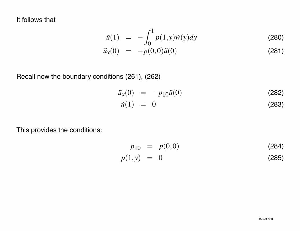
It follows that

u(1) = &Z 1

0p(1,y)w(y)dy (280)

ux(0) = &p(0,0)u(0) (281)

Recall now the boundary conditions (261), (262)

ux(0) = &p10u(0) (282)u(1) = 0 (283)

This provides the conditions:

p10 = p(0,0) (284)p(1,y) = 0 (285)

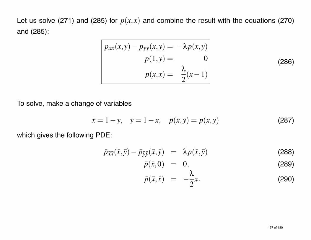
Let us solve (271) and (285) for p(x,x) and combine the result with the equations (270)and (285):

pxx(x,y)& pyy(x,y) = &"p(x,y)p(1,y) = 0

p(x,x) ="2(x&1)

(286)

To solve, make a change of variables

x= 1& y, y= 1& x, p(x, y) = p(x,y) (287)

which gives the following PDE:

pxx(x, y)& pyy(x, y) = "p(x, y) (288)p(x,0) = 0, (289)

p(x, x) = &"2x . (290)

The solution is

p(x, y) = &"yI1(

3

"(x2& y2))3

"(x2& y2). (291)

or, in the original variables,

p(x,y) = &"(1& x)I1(

&

"(2& x& y)(x& y))&

"(2& x& y)(x& y). (292)

The observer gains,obtained using (272) and (284) are

p1(x) = py(x,0) ="(1& x)x(2& x)

I2$&

"x(2& x)%

(293)

p10 = p(0,0) = &"2. (294)

Summary of the plant and observer

Plant ut = uxx+"u (295)ux(0) = 0 (296)u(1) =U (297)

Observer ut = uxx+"u +"(1& x)x(2& x)

I2$&

"x(2& x)%

[u(0)& u(0)] (298)

ux(0) = &"2

[u(0)& u(0)] (299)

u(1) =U (300)

Output Feedback

The observer can be used with any controller.

For linear systems, the separation principle (or “certainty equivalence”) holds, i.e. thecombination of a separately designed state feedback controller and observer results in astabilizing output-feedback controller.

Next, we establish the separation principle for our observer-based output feedback design.

The control backstepping transformation u /+ w (on the state estimate)

w(x) = u(x)&Z x

0k(x,y)u(y)dy (direct) (301)

u(x) = w(x)+Z x

0l(x,y)w(y)dy (inverse) (302)

and the observer backstepping transformation u /+ w

u(x) = w(x)&Z x

0p(x,y)w(y)dy (inverse) (303)

map the closed-loop sys into a target system of cascade form w+ w

wt = wxx+

'

p1(x)&Z x

0k(x,y)p1(y)dy

(

w(0) (304)

wx(0) = p10w(0) (305)w(1) = 0 (306)

wt = wxx (307)wx(0) = 0 AUTONOMOUS SYST. (308)w(1) = 0, (309)

where k(x,y) is the kernel of the control transformation and p1(x), p10 are observer gains.

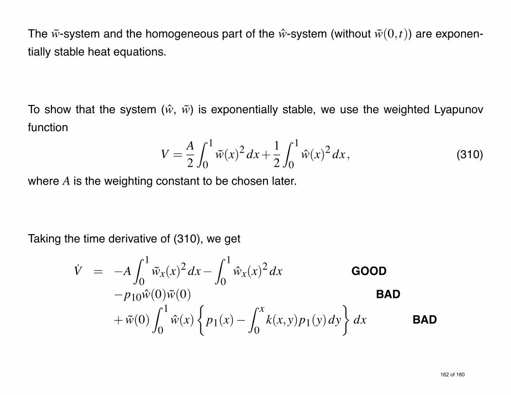
The w-system and the homogeneous part of the w-system (without w(0, t)) are exponen-tially stable heat equations.

To show that the system (w, w) is exponentially stable, we use the weighted Lyapunovfunction

V =A2

Z 1

0w(x)2dx+

12

Z 1

0w(x)2dx , (310)

where A is the weighting constant to be chosen later.

Taking the time derivative of (310), we get

V = &AZ 1

0wx(x)2dx&

Z 1

0wx(x)2dx GOOD

&p10w(0)w(0) BAD

+ w(0)Z 1

0w(x)

'

p1(x)&Z x

0k(x,y)p1(y)dy

(

dx BAD

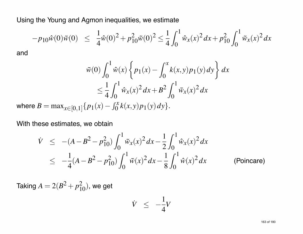
Using the Young and Agmon inequalities, we estimate

&p10w(0)w(0) %14w(0)2+ p210w(0)2 %

14

Z 1

0wx(x)2dx+ p210

Z 1

0wx(x)2dx

and

w(0)Z 1

0w(x)

'

p1(x)&Z x

0k(x,y)p1(y)dy

(

dx

%14

Z 1

0wx(x)2dx+B2

Z 1

0wx(x)2dx

where B=maxx"[0,1]{p1(x)&R x0 k(x,y)p1(y)dy}.

With these estimates, we obtain

V % &(A&B2& p210)Z 1

0wx(x)2dx&

12

Z 1

0wx(x)2dx

% &14(A&B2& p210)

Z 1

0w(x)2dx&

18

Z 1

0w(x)2dx (Poincare)

Taking A= 2(B2+ p210), we get

V % &14V

Hence, the system (w, w) is exponentially stable.

The system (u, u) is also exponentially stable since it is related to (w, w) by the invertiblecoordinate transformations (303) and (302).

We have proved the separation principle.

Output feedback design for anti-collocated setup

Plant ut = uxx+"u (311)ux(0) = 0 (312)

Observer ut = uxx+"u+"(1& x)x(2& x)

I2$&

"x(2& x)%

[u(0)& u(0)] (313)

ux(0) = &"2[u(0)& u(0)] (314)

u(1) = &Z 1

0"I1(

3

"(1& y2))3

"(1& y2)u(y)dy (315)

Controller u(1) = &Z 1

0"I1(

3

"(1& y2))3

"(1& y2)u(y)dy (316)

Observer Design for Collocated Sensor and Actuator

ut = uxx+"u (317)ux(0) = 0 (318)u(1) = U(t) (319)ux(1) & measurement

Observer

ut = uxx+"u+ p1(x)[ux(1)& ux(1)] (320)ux(0) = 0 (321)u(1) = U(t)+ p10[ux(1)& ux(1)] (322)

Error u= u& u, error system

ut = uxx+"u& p1(x)ux(1) (323)ux(0) = 0 (324)u(1) = &p10ux(1) (325)

Backstepping transformation

u(x) = w(x)&Z 1

xp(x,y)w(y)dy (326)

to convert the error system into target system:

wt = wxx (327)wx(0) = 0 (328)w(1) = 0. (329)

Note that the integral in the transformation runs from x to 1 instead of the usual 0 to x!

We get the kernel PDE

pxx(x,y)& pyy(x,y) = &"p(x,y) (330)px(0,y) = 0, (331)

p(x,x) = &"2x (332)

From the resulting target system

wt = wxx+[p(x,1)& p1(x)]wx(1) (333)wx(0) = 0 (334)w(1) = &p10wx(1) (335)

the observer gains should be chosen as

p1(x) = p(x,1), p10 = 0. (336)

To solve the kernel PDE (330)–(332) we introduce the change of variables

x= y, y= x, p(x, y) = p(x,y)

to get

pxx(x, y)& pyy(x, y) = "p(x, y) (337)py(x,0) = 0, (338)

p(x, x) = &"2x . (339)

This PDE’s solution is

p(x, y) = &"xI1(

3

"(x2& y2))3

"(x2& y2)

= &"yI1(

3

"(y2& x2))3

"(y2& x2)

Therefore, the observer gains are

p1(x) = &"I1(

3

"(1& x2))3

"(1& x2)(340)

and p10 = 0.

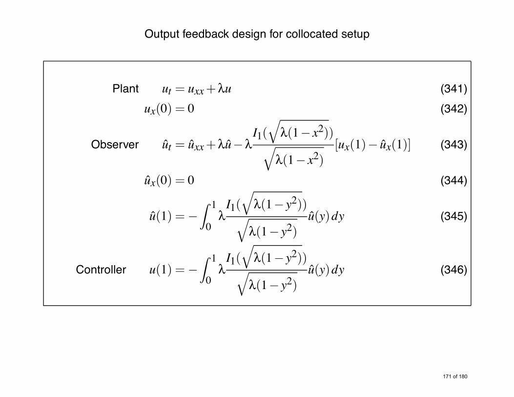
Output feedback design for collocated setup

Plant ut = uxx+"u (341)ux(0) = 0 (342)

Observer ut = uxx+"u&"I1(

3

"(1& x2))3

"(1& x2)[ux(1)& ux(1)] (343)

ux(0) = 0 (344)

u(1) = &Z 1

0"I1(

3

"(1& y2))3

"(1& y2)u(y)dy (345)

Controller u(1) = &Z 1

0"I1(

3

"(1& y2))3

"(1& y2)u(y)dy (346)

The fact that p1(x) = k(1,x) demonstrates the duality between observer and control de-signs, the property known from the finite-dimensional designs for linear systems.

We used the same decay rates for the observer and controller. One can easily modify thedesigns to make the observer faster that the controller.

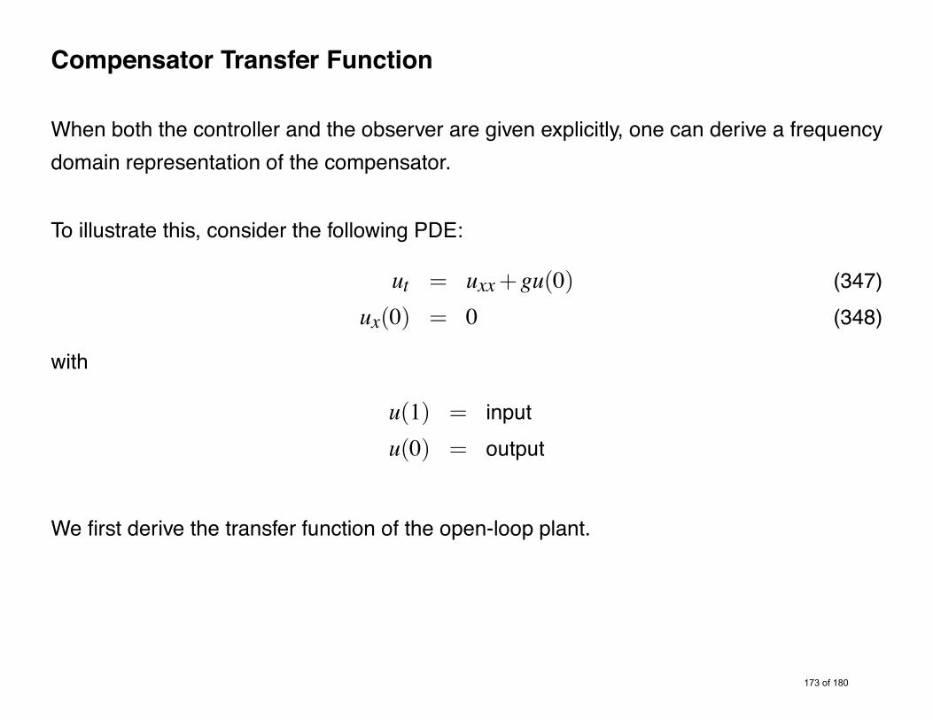
Compensator Transfer Function

When both the controller and the observer are given explicitly, one can derive a frequencydomain representation of the compensator.

To illustrate this, consider the following PDE:

ut = uxx+gu(0) (347)ux(0) = 0 (348)

with

u(1) = inputu(0) = output

We first derive the transfer function of the open-loop plant.

Taking the Laplace transform of (347), (348) we get

su(x,s) = u**(x,s)+gu(0,s) (349)u*(0,s) = 0 (350)

The general solution for this second order ODE in x is given by

u(x,s) = Asinh(-sx)+Bcosh(

-sx)+

gsu(0,s) , (351)

where A and B are to be determined. From the boundary condition (350) we have

u*(0,s) = A-s= 0, A= 0 . (352)

By setting x= 0 in (351), we find B:

B= u(0,s)$

1&gs

%

. (353)

Hence, we get

u(x,s) = u(0,s))gs

$

1&gs

%

cosh(-sx)

*

.

Setting x= 1 we obtain the plant transfer function

u(0,s) =s

g+(s&g)cosh(-s)u(1,s) (354)

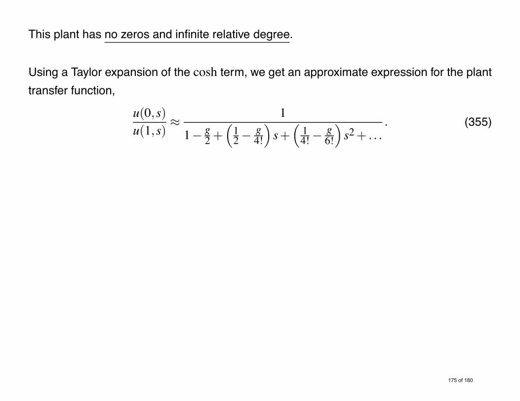
This plant has no zeros and infinite relative degree.

Using a Taylor expansion of the cosh term, we get an approximate expression for the planttransfer function,

u(0,s)u(1,s)

01

1& g2+

$12&

g4!

%

s+$14!&

g6!

%

s2+ . . .. (355)

Let us now derive the frequency domain representation of the compensator.

The observer PDE is given by

ut = uxx+gu(0) (356)ux(0) = 0 (357)

u(1) = &Z 1

0

-gsinh(

-g(1& y))u(y)dy . (358)

Applying the Laplace transform, we get

su(x,s) = u**(x,s)+gu(0,s) (359)u*(0,s) = 0 (360)

u(1,s) = &Z 1

0

-gsinh(

-g(1& y))u(y,s)dy (361)

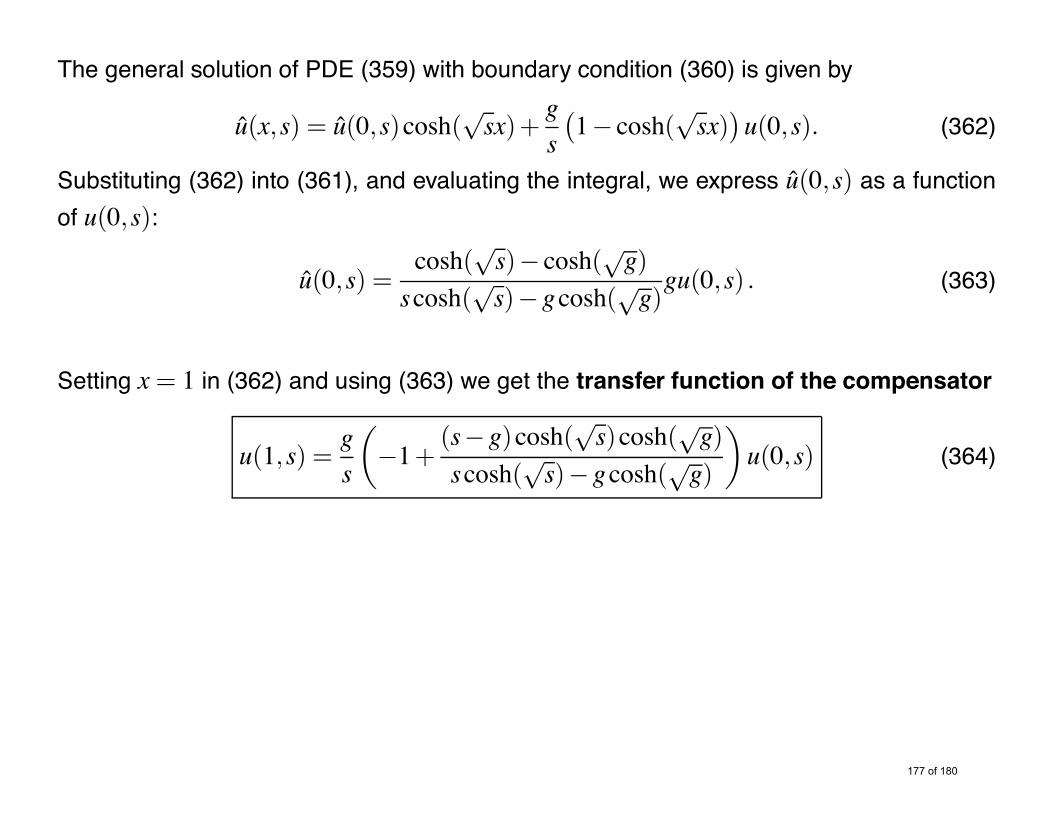
The general solution of PDE (359) with boundary condition (360) is given by

u(x,s) = u(0,s)cosh(-sx)+

gs/

1& cosh(-sx)

0

u(0,s). (362)

Substituting (362) into (361), and evaluating the integral, we express u(0,s) as a functionof u(0,s):

u(0,s) =cosh(

-s)& cosh(-g)

scosh(-s)&gcosh(-g)

gu(0,s) . (363)

Setting x= 1 in (362) and using (363) we get the transfer function of the compensator

u(1,s) =gs

!

&1+(s&g)cosh(

-s)cosh(-g)

scosh(-s)&gcosh(-g)

"

u(0,s) (364)

10−1 100 101 102 103−30

−20

−10

0

10

20

Mag

nitu

de (

dB)

0 , rad/sec 10−1 100 101 102 103−90

−75

−60

−45

−30

−15

0

Phas

e (d

eg)

0 , rad/sec

Bode plots of the compensator (364)

Compensator can be approximated by a second order, relative degree one transfer func-tion, for example,

C(s) 0 60s+17

s2+25s+320. (365)

Homework

1. Design an observer for the following system:

ut = uxxux(0) = &qu(0)u(1) = U(t)

with only ux(1) available for measurement.

Follow these steps:

1) Write down the observer for this system, with output injection entering the PDE andthe boundary condition at x= 1.

2) Use the transformation

u(x) = w(x)&Z 1

xp(x,y)w(y)dy (366)

to map the error system into the target system

wt = wxx (367)wx(0) = 0 (368)w(1) = 0 . (369)

Show that p(x,y) satisfies the PDE

pxx(x,y) = pyy(x,y) (370)px(0,y) = &qp(0,y) (371)p(x,x) = &q . (372)

and that the observer gains are given by p10 = 0 and p1(x) = p(x,1).

3) Solve the PDE for p(x,y) (look for the solution in the form p(x,y) = .(y& x)). Findp1(x).

2. Find the frequency domain representation of the plant

ut = uxxux(0) = &qu(0)u(1) = U(t)

with u(0) measured and u(1) actuated, i.e., find G(s) such that u(0,s) = G(s)U(s).