Rewriting Polynomials - University of Illinois at Chicagohomepages.math.uic.edu/~jan/mcs563/rewriting.pdf · Rewriting Polynomials 1 Roots and Eigenvalues the companion matrix of

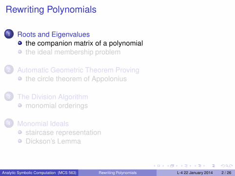
Rewriting Polynomials

1 Roots and Eigenvaluesthe companion matrix of a polynomialthe ideal membership problem

2 Automatic Geometric Theorem Provingthe circle theorem of Appolonius

3 The Division Algorithmmonomial orderings

4 Monomial Idealsstaircase representationDickson’s Lemma

MCS 563 Lecture 4Analytic Symbolic Computation

Jan Verschelde, 22 January 2014

Analytic Symbolic Computation (MCS 563) Rewriting Polynomials L-4 22 January 2014 1 / 26







roots and eigenvalues

For example, consider

p(x) = x4 − 5x3 + 7x2 − x + 3 ∈ C[x ]= (x − z1)(x − z2)(x − z3)(x − z4),

we can identify p with its roots z1, z2, z3, z4.

Algebraically, p(x) = 0 implies

x4 = 5x3 − 7x2 + x − 3.

As x4 is a linear combination of 1, x , x2, x3,we can also write x5, x6, etc. as cubic polynomials.


the quotient ring

The relationx4 = 5x3 − 7x2 + x − 3

maps every polynomial in C[x ] onto the quotient ring

C[x ]/〈p〉 = { a0 + a1x + a2x2 + a3x3 | ai ∈ C },

is a 4-dimensional vector space with basis {1, x , x2, x3}.

By this vector space a problem of polynomial algebra becomes aproblem of linear algebra.


the companion matrix

The relationx4 = 5x3 − 7x2 + x − 3

as a matrix equation

x

1xx2

x3

=

0 1 0 00 0 1 00 0 0 1

−3 1 −7 5

1xx2

x3

.

The matrix above is the companion matrix Cp of p.

Denote by X = [1 x x2 x3]T and use λ for x , then

λX = CpX

⇒ the 4 eigenvalues of Cp are the 4 roots of p.








the ideal generated by f

For a system f (x) = 0, with f = (f1, f2, . . . , fN),we define the ideal generated by f as

〈f 〉 = { a1f1 + a2f2 + · · ·+ aNfN | ai ∈ C[x] }.The ideal membership problem: for a given ideal I and polynomial p,determine whether p ∈ I.

The solution to the membership problem is the map

C[x ] → C[x ]/Ip �→ p mod I

where p mod I is p modulo the ideal I.

If we can rewrite (or reduce) p modulo I in a unique way thenp mod I = 0 ⇔ p ∈ I.








the circle theorem of Appolonius

A � B�

C ��

M2�

M1�

M3�

H�

��

Theorem (The Circle Theorem of Appolonius)Consider a right triangle spanned by A, B, and C, with the right angleat A. The midpoints of the three sides of the triangle, and the foot ofthe altitude drawn from A to the edge spanned by B and C all lie onone circle.


coordinates and equations

The triangle spanned by A, B, C has midpoints M1, M2, M3:Corners: A = (0,0), B = (u1,0), and C = (0,u2), where u1 and u2are arbitrary.Midpoints: M1 = (x1,0), M2 = (0, x2), M3 = (x3, x4).

M1 is the midpoint of the edge spanned by A and B

h1 = 2x1 − u1 = 0.

Similarly, h2 = 2x2 − u2 = 0 expresses thatM2 is the midpoint of the edge spanned by A and C.

For M3 we have two conditions:

h3 = 2x3 − u1 = 0 and h4 = 2x4 − u2 = 0.


coordinates and hypotheses

For the foot of the altitude H we choose coordinates (x5, x6).The line segment AH is perpendicular to the edge BC:

h5 = x5u1 − x6u2 = 0.

The points B, H, and C are collinear:

h6 = x5u2 + x6u1 − u1u2 = 0.

The circle through the three midpoints must also contain H.Let (x7, x8) be the coordinates of the center O of the circle.M1O = M2O and M1O = M3O is respectively equal toh7 = (x1 − x7)

2 + x28 − x2

7 − (x8 − x2)2 = 0 and

h8 = (x1 − x7)2 + x2

8 − (x3 − x7)2 − (x4 − x8)

2 = 0.


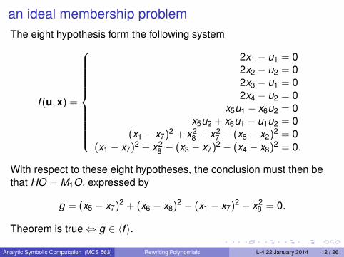
an ideal membership problemThe eight hypothesis form the following system

f (u,x) =

2x1 − u1 = 02x2 − u2 = 02x3 − u1 = 02x4 − u2 = 0

x5u1 − x6u2 = 0x5u2 + x6u1 − u1u2 = 0

(x1 − x7)2 + x2

8 − x27 − (x8 − x2)

2 = 0(x1 − x7)

2 + x28 − (x3 − x7)

2 − (x4 − x8)2 = 0.

With respect to these eight hypotheses, the conclusion must then bethat HO = M1O, expressed by

g = (x5 − x7)2 + (x6 − x8)

2 − (x1 − x7)2 − x2

8 = 0.

Theorem is true ⇔ g ∈ 〈f 〉.Analytic Symbolic Computation (MCS 563) Rewriting Polynomials L-4 22 January 2014 12 / 26







quotient and remainder

We want to solve the ideal membership problem.

For g ∈ C[x] and an ideal generated by f = (f1, f2, . . . , fN):

Findqi ∈ C[x], i = 1,2, . . . ,N and r ∈ C[x]

so thatg = q1f1 + q2f2 + · · ·+ qNfN + r .

Obviously, if r = 0, then g ∈ 〈f 〉,but the opposite is not necessarily true.


ordering monomials

First, order the variables: x1 > x2 > · · · > xn.Then, there are several monomial orderings:

lexicographic: We sort as in a dictionary.xa >lex xb if the leftmost nonzero entry in a − b is positive. Forexample: x2

1 x2 >lex x1x32 .

graded lexicographic: We first sort the monomials according totheir total degree and sort monomials with the same degreelexicographically. We have xa >tdeg xb if deg(xa) > deg(xb) or ifdeg(xa) = deg(xb) and xa >lex xb. For example: x2

1 x2 >tdeg x1x22 .

weighted lexicographic: For ω ∈ Zn \ {0}, denote

〈a, ω〉 = a1ω1 + a2ω2 + · · · + anωn. Then: xa >ω xb if〈a, ω〉 > 〈b, ω〉 or 〈a, ω〉 = 〈b, ω〉 and xa >lex xb.

Denote the leading term of a polynomial g by LT(g).


the division algorithmThe division algorithm to compute the remainder:

Input: f = (f1, f2, . . . , fN) and p ∈ C[x].Output: r , the remainder of p modulo f , denoted by p →f r .

r := p;repeat

k := 0;for i from 1 to N do

if LT(fi) divides LT(r)then k := i ; exit for loop;end if;

end for;

if k �= 0 then r := r − LT(r)LT(fk )

fk ; end if;

until r = 0 or k = 0.


an example

Take >lex as monomial order and g = xy2 − x with respect to the idealgenerated by f1 = xy + 1 and f2 = y2 − 1.

〈f1, f2〉 : LT(g) = yLT(f1) → g := g − yf1= xy2 − x − y(xy + 1)= −x − y .

But when we swap the order of the polynomials in 〈f 〉:

〈f2, f1〉 : LT(g) = xLT(f2) → g := g − xf2= xy2 − x − x(y2 − x)= 0,

we see that g ∈ 〈f 〉.








monomial ideals

A monomial ideal is generated by monomials.

For example: 〈x2y5, x3y4, x4y2〉.Identifying exponents with lattice points,leads to a staircase:

�1

�

1

� � � � � � � �

� � � � � � � �

� � � � � � � �

� � � � � � � �

� � � � � � �

� � � � � �

� � � � ��








Dickson’s Lemma

Lemma (Dickson’s Lemma)Every monomial ideal is finitely generated.

Proof. We need to show that for every monomial ideal I,

there exists a finite subset S so that

for all xa ∈ I there is a monomial xb ∈ S that divides xa.

We proceed by induction on n, the number of variables.

For n = 1, d = minxa∈I

xa is unique, so S = {xd}.


applying induction

For n > 1, take xb ∈ I. Every monomial in I not divisible by xb belongsto one of the following sets:

Ri ,j = { xa ∈ I | ai = j }, i = 1,2, . . . ,n, j = 0,1, . . . ,bi − 1.

Denote Ri ,j = { xa|xi=1 | xa ∈ Ri ,j } (xi removed from Ri ,j).

By the induction hypothesis, there is a finite set Si ,j that generatesIi = { xa|xi=1 | xa ∈ I }.

Define Si ,j = { xji x

a | xa ∈ Si ,j } and let

S = {xb} ∪ n⋃

i=1

bi−1⋃j=0

Si ,j

.

S generates xb and every xa ∈ I not divisible by xb.Thus S generates I.


Groebner Basis

A Groebner basis G for an ideal I is1 a basis for the ideal, i.e.: 〈G〉 = I;2 the output of the division algorithm is unique: p →G= p →I .

With a Groebner basis G for I, the r in p →G ris the normal form of p with respect to I.

An algorithm to compute a Groebner basis leads to

Theorem (Hilbert’s basis theorem)Every ideal has a finite generating set.


Summary + Exercises

We introduced the division algorithm and defined the idealmembership problem.

Exercises:1 For the polynomial p(x) = x4 − 5x3 + 7x2 − x + 3, use MATLAB

(Octave will do as well) or Maple to define the companion matrixand to compute its eigenvalues. What are the eigenvectors?

2 Consider the polynomial p(x) = (x − 1)3(x − 2) and describe theeigenvalues and eigenvectors of the companion matrix, usingMATLAB or Maple. Can you recognize the multiplicies of the tworoots?


more exercises

3 Write a Maple procedure to implement the division algorithm.Extend your implementation so that in addition to the remainder rthe algorithm also returns the “quotients” qi in the combinationf = q1g1 + q2g2 + · · · + qNgN + r , for any basis g and inputpolynomial f . You may also use another computer algebra system.

4 Consider the monomial ideal I = 〈x3y , x2y2, xy6〉. Draw theexponent vectors of the monomials in the plane and visualize thestaircase and all elements generated by I.

5 How can you see from the staircase that the monomial ideal hasonly finitely many solutions? Give examples and justify yourobservation.


and more exercises

6 For some finite support set A, let I = 〈xa | a ∈ A〉 be the monomialideal defined by A. Show that xb ∈ I if and only if xb is divisible bysome monomial xa for some a ∈ A.

7 Let f = (xa1 ,xa2 , . . . ,xaN ) define a monomial ideal. Show thatp ∈ 〈f 〉 ⇔ p →f 0.

8 Use Maple or Sage (in particular: Singular) to compute aGroebner basis of the ideal generated by the polynomial in thesystem f (u,x) (of the circle theorem of Appolonius), using alexicographic order on the monomials. Does the form of theGroebner basis allow you to reduce the conclusion g to zero?


Documents

Rewriting Polynomials - University of Illinois at Chicagohomepages.math.uic.edu/~jan/mcs563/rewriting.pdf · Rewriting Polynomials 1 Roots and Eigenvalues the companion matrix of