Gröbner Bases - University of Illinois at Chicagohomepages.math.uic.edu/~jan/mcs563/groebner.pdf · Gröbner Bases 1 S-polynomials eliminating the leading term Buchberger’s criterion

Gröbner Bases

1 S-polynomialseliminating the leading termBuchberger’s criterion and algorithm

2 Wavelet Designconstruct wavelet filters

3 Proof of the Buchberger Criteriontwo lemmasproof of the Buchberger criteriontermination and elimination

MCS 563 Lecture 6Analytic Symbolic Computation

Jan Verschelde, 27 January 2014

Analytic Symbolic Computation (MCS 563) Gröbner Bases L-6 27 January 2014 1 / 31

Gröbner Bases





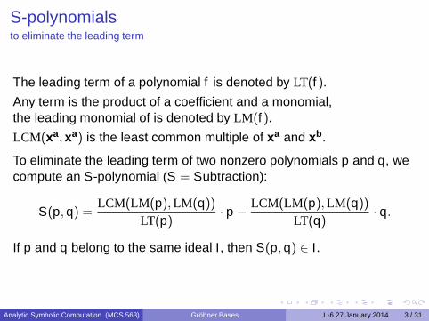
S-polynomialsto eliminate the leading term

The leading term of a polynomial f is denoted by LT(f ).

Any term is the product of a coefficient and a monomial,the leading monomial of is denoted by LM(f ).

LCM(xa, xa) is the least common multiple of xa and xb.

To eliminate the leading term of two nonzero polynomials p and q, wecompute an S-polynomial (S = Subtraction):

S(p, q) =LCM(LM(p), LM(q))

LT(p)· p −

LCM(LM(p), LM(q))

LT(q)· q.

If p and q belong to the same ideal I, then S(p, q) ∈ I.


an example

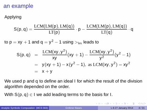
Applying

S(p, q) =LCM(LM(p), LM(q))

LT(p)· p −

LCM(LM(p), LM(q))

LT(q)· q

to p = xy + 1 and q = y2 − 1 using >lex leads to

S(p, q) =LCM(xy , y2)

xy(xy + 1) −

LCM(xy , y2)

y2 (y2 − 1)

= y(xy + 1) − x(y2 − 1), as LCM(xy , y2) = xy2

= x + y

We used p and q to define an ideal I for which the result of the divisionalgorithm depended on the order.

With S(p, q) ∈ I we add leading terms to the basis for I.


Gröbner Bases





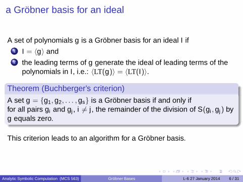
a Gröbner basis for an ideal

A set of polynomials g is a Gröbner basis for an ideal I if1 I = 〈g〉 and2 the leading terms of g generate the ideal of leading terms of the

polynomials in I, i.e.: 〈LT(g)〉 = 〈LT(I)〉.

Theorem (Buchberger’s criterion)

A set g = {g1, g2, . . . , gs} is a Gröbner basis if and only iffor all pairs gi and gj , i 6= j , the remainder of the division of S(gi , gj) byg equals zero.

This criterion leads to an algorithm for a Gröbner basis.


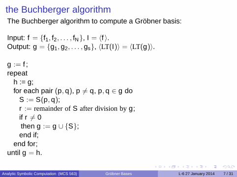
the Buchberger algorithmThe Buchberger algorithm to compute a Gröbner basis:

Input: f = {f1, f2, . . . , fN}, I = 〈f 〉.Output: g = {g1, g2, . . . , gs}, 〈LT(I)〉 = 〈LT(g)〉.

g := f ;repeat

h := g;for each pair (p, q), p 6= q, p, q ∈ g do

S := S(p, q);r := remainder of S after division by g;if r 6= 0then g := g ∪ {S};end if;

end for;until g = h.


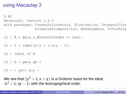
using Macaulay 2

$ M2Macaulay2, version 1.3.1with packages: ConwayPolynomials, Elimination, IntegralClosure,

PrimaryDecomposition, ReesAlgebra, SchurRings,

i1 : R = QQ[x,y,MonomialOrder => Lex];

i2 : I = ideal(x^2 + 1,x*y - 1);

o2 : Ideal of R

i3 : G = gens gb I

o3 = | y2+1 x+y |

We see that {y2 + 1, x + y} is a Gröbner basis for the ideal〈x2 + 1, xy − 1〉 with the lexicographical order.


some more Gröbner basics

Buchberger’s algorithm generalizes Euclid’s algorithm for the GCD androw reduction for linear systems.

With a Gröbner bases, the division algorithm solvesthe ideal membership problem.

A Gröbner basis g is called reduced if1 the leading coefficient of every polynomial in g is 1; and2 for all p ∈ g, no monomial of p lies in 〈LT(g \ {p})〉.

Fixing a monomial order,any nonzero ideal has a unique reduced Gröbner basis.


Gröbner Bases





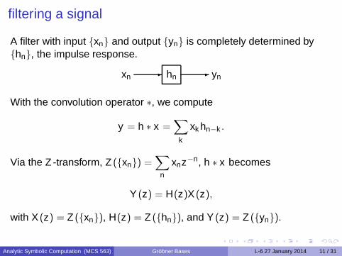
filtering a signal

A filter with input {xn} and output {yn} is completely determined by{hn}, the impulse response.

xn- hn

- yn

With the convolution operator ∗, we compute

y = h ∗ x =∑

k

xk hn−k .

Via the Z -transform, Z ({xn}) =∑

n

xnz−n, h ∗ x becomes

Y (z) = H(z)X (z),

with X (z) = Z ({xn}), H(z) = Z ({hn}), and Y (z) = Z ({yn}).


filter design

The function H(z) is called the transfer function of the filter.

We design a filter by determination of H.

Example of conditions on the transfer function:

1 h2 = h3, h1 = h4;2 (z + 1)2 divides H(z);

3∑

n

hnhn−2k = δ(k),

with δ(k) = 1 if k = 0, δ(k) = 0 if k 6= 0.


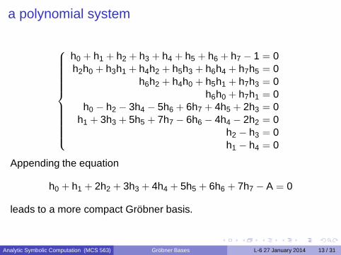
a polynomial system

h0 + h1 + h2 + h3 + h4 + h5 + h6 + h7 − 1 = 0h2h0 + h3h1 + h4h2 + h5h3 + h6h4 + h7h5 = 0

h6h2 + h4h0 + h5h1 + h7h3 = 0h6h0 + h7h1 = 0

h0 − h2 − 3h4 − 5h6 + 6h7 + 4h5 + 2h3 = 0h1 + 3h3 + 5h5 + 7h7 − 6h6 − 4h4 − 2h2 = 0

h2 − h3 = 0h1 − h4 = 0

Appending the equation

h0 + h1 + 2h2 + 3h3 + 4h4 + 5h5 + 6h6 + 7h7 − A = 0

leads to a more compact Gröbner basis.


Gröbner Bases





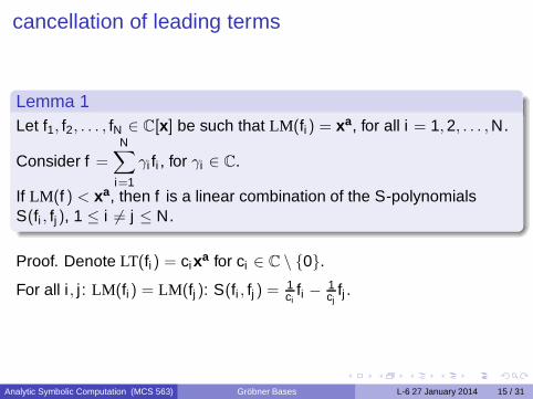
cancellation of leading terms

Lemma 1Let f1, f2, . . . , fN ∈ C[x] be such that LM(fi) = xa, for all i = 1, 2, . . . , N.

Consider f =

N∑

i=1

γi fi , for γi ∈ C.

If LM(f ) < xa, then f is a linear combination of the S-polynomialsS(fi , fj), 1 ≤ i 6= j ≤ N.

Proof. Denote LT(fi) = cixa for ci ∈ C \ {0}.

For all i , j : LM(fi) = LM(fj ): S(fi , fj ) = 1ci

fi − 1cj

fj .


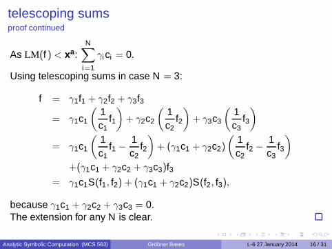
telescoping sumsproof continued

As LM(f ) < xa:N∑

i=1

γici = 0.

Using telescoping sums in case N = 3:

f = γ1f1 + γ2f2 + γ3f3

= γ1c1

(1c1

f1

)+ γ2c2

(1c2

f2

)+ γ3c3

(1c3

f3

)

= γ1c1

(1c1

f1 −1c2

f2

)+ (γ1c1 + γ2c2)

(1c2

f2 −1c3

f3

)

+(γ1c1 + γ2c2 + γ3c3)f3= γ1c1S(f1, f2) + (γ1c1 + γ2c2)S(f2, f3),

because γ1c1 + γ2c2 + γ3c3 = 0.The extension for any N is clear.


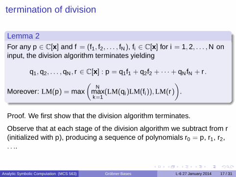
termination of division

Lemma 2For any p ∈ C[x] and f = (f1, f2, . . . , fN), fi ∈ C[x] for i = 1, 2, . . . , N oninput, the division algorithm terminates yielding

q1, q2, . . . , qN , r ∈ C[x] : p = q1f1 + q2f2 + · · · + qN fN + r .

Moreover: LM(p) = max(

Nmaxk=1

(LM(qi)LM(fi)), LM(r))

.

Proof. We first show that the division algorithm terminates.

Observe that at each stage of the division algorithm we subtract from r(initialized with p), producing a sequence of polynomials r0 = p, r1, r2,. . ..


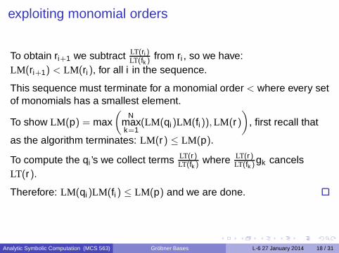
exploiting monomial orders

To obtain ri+1 we subtract LT(ri )LT(fk ) from ri , so we have:

LM(ri+1) < LM(ri), for all i in the sequence.

This sequence must terminate for a monomial order < where every setof monomials has a smallest element.

To show LM(p) = max(

Nmaxk=1

(LM(qi)LM(fi)), LM(r))

, first recall that

as the algorithm terminates: LM(r) ≤ LM(p).

To compute the qi ’s we collect terms LT(r)LT(fk ) where LT(r)

LT(fk )gk cancelsLT(r).

Therefore: LM(qi)LM(fi ) ≤ LM(p) and we are done.


Gröbner Bases





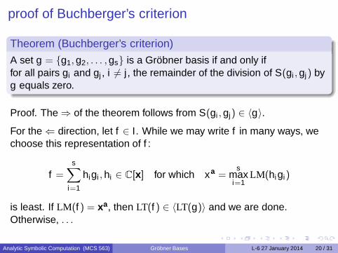
proof of Buchberger’s criterion

Theorem (Buchberger’s criterion)

A set g = {g1, g2, . . . , gs} is a Gröbner basis if and only iffor all pairs gi and gj , i 6= j , the remainder of the division of S(gi , gj) byg equals zero.

Proof. The ⇒ of the theorem follows from S(gi , gj) ∈ 〈g〉.

For the ⇐ direction, let f ∈ I. While we may write f in many ways, wechoose this representation of f :

f =s∑

i=1

higi , hi ∈ C[x] for which xa =s

maxi=1

LM(higi)

is least. If LM(f ) = xa, then LT(f ) ∈ 〈LT(g)〉 and we are done.Otherwise, . . .


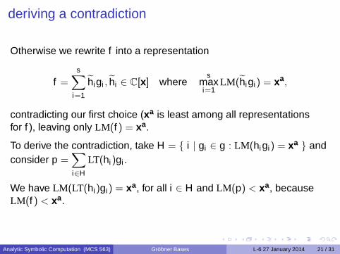
deriving a contradiction

Otherwise we rewrite f into a representation

f =

s∑

i=1

h̃igi , h̃i ∈ C[x] wheres

maxi=1

LM(h̃igi) = xa,

contradicting our first choice (xa is least among all representationsfor f ), leaving only LM(f ) = xa.

To derive the contradiction, take H = { i | gi ∈ g : LM(higi) = xa } andconsider p =

∑

i∈H

LT(hi)gi .

We have LM(LT(hi)gi) = xa, for all i ∈ H and LM(p) < xa, becauseLM(f ) < xa.


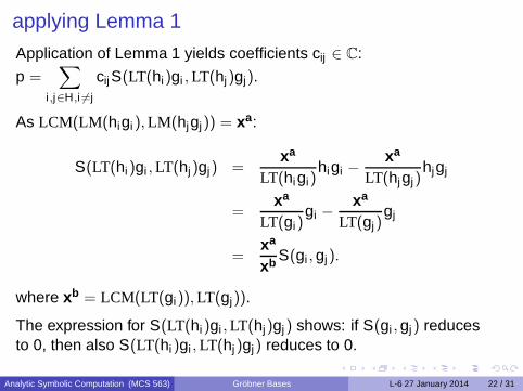
applying Lemma 1

Application of Lemma 1 yields coefficients cij ∈ C:

p =∑

i ,j∈H,i 6=j

cijS(LT(hi)gi , LT(hj)gj).

As LCM(LM(higi), LM(hjgj)) = xa:

S(LT(hi)gi , LT(hj)gj) =xa

LT(higi)higi −

xa

LT(hjgj)hjgj

=xa

LT(gi)gi −

xa

LT(gj)gj

=xa

xb S(gi , gj).

where xb = LCM(LT(gi)), LT(gj)).

The expression for S(LT(hi)gi , LT(hj)gj) shows: if S(gi , gj) reducesto 0, then also S(LT(hi)gi , LT(hj)gj) reduces to 0.


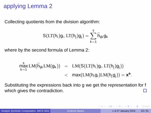
applying Lemma 2

Collecting quotients from the division algorithm:

S(LT(hi)gi , LT(hj)gj) =

s∑

k=1

h̃ijkgk

where by the second formula of Lemma 2:

smaxk=1

LM(h̃ijk LM(gk )) = LM(S(LT(hi)gi , LT(hj)gj))

< max(LM(higi)LM(hjgj)) = xa.

Substituting the expressions back into g we get the representation for fwhich gives the contradiction.


Gröbner Bases





the Buchberger algorithm terminates

Showing that this algorithm terminates also shows the Hilbert basistheorem, i.e.: any ideal has a finite basis.

The key observation is that as long as the repeat loop does notterminate, we augment g with a nonzero polynomial S = S(p, q) forwhich LM(S) < LM(p) and LM(S) < LM(q), with respect to the termorder <.

Compared to h, we thus have that 〈LT(h)〉 ⊂ 〈LT(g)〉.

So as long as the loop runs, we create a chain of monomial idealswhich cannot stretch for ever.


Elimination Ideals

Consider again a system of homogeneous linear equations.Applying row reduction to bring such a system into triangular form canbe written in terms of taking S-polynomials.

For an ideal I in C[x], x = (x1, x2, . . . , xn), the k th elimination ideal isIk = I ∩ C[xk+1, . . . , xn].

So Ik consists of all polynomials in I for which the first k variables havebeen eliminated.

Theorem (The Elimination Theorem)Let g be a Gröbner basis for an ideal I with respect to the purelexicographical order x1 > x2 > · · · > xn. Then the setgk = g ∩ C[xk+1, . . . , xn] is a Gröbner basis of the kth eliminationideal Ik .


proof of the Elimination theorem

Proof. To prove this theorem, we must show that 〈LT(Ik )〉 = 〈LT(gk )〉.By construction, 〈LT(gk )〉 ⊂ 〈LT(Ik )〉, so what remains to show is that〈LT(Ik )〉 ⊂ 〈LT(gk )〉.

For any f ∈ Ik , we must then show that LT(f ) is divisible by LT(p) forsome p ∈ gk .

As f ∈ I: LT(f ) is divisible by LT(p) for some p ∈ g.Since f ∈ Ik , the only variables in f are xk+1, . . . , xn.

Because of the lexicographic order: if LT(p) ∈ C[xk+1, . . . , xn], then allother terms of p also ∈ C[xk+1, . . . , xn].

Thus the p for which LT(p) divides LT(f ) belongs to gk .


Summary + Exercises

We gave a definition for the Gröbner basis, explained Buchberger’scriterion and algorithm.

Exercises:1 Solve the system for filter design. Use Maple or Sage to create a

lexicographical Gröbner basis. Verify that by adding one moreequation, the resulting Gröbner basis is more compact. How manyreal solutions do you find?

2 Apply Buchberger’s algorithm by hand (you can use a Mapleworksheet to compute all S-polynomials) to the ideal generated bythe equations {x2

1 + x22 − 1, x1x2 − 1} using a pure lexicographical

monomial order.3 Show that for two systems f (x) = 0 and g(x) = 0: if 〈f 〉 = 〈g〉,

then their solutions are the same. Give an example of a case forwhich the opposite direction does hold.


more exercises

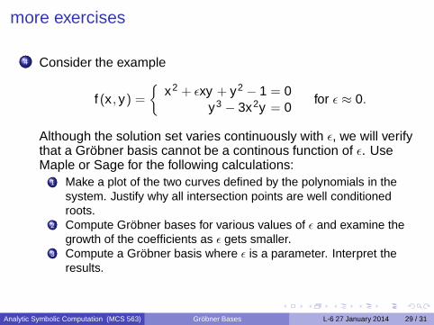
4 Consider the example

f (x , y) =

{x2 + ǫxy + y2 − 1 = 0

y3 − 3x2y = 0for ǫ ≈ 0.

Although the solution set varies continuously with ǫ, we will verifythat a Gröbner basis cannot be a continous function of ǫ. UseMaple or Sage for the following calculations:

1 Make a plot of the two curves defined by the polynomials in thesystem. Justify why all intersection points are well conditionedroots.

2 Compute Gröbner bases for various values of ǫ and examine thegrowth of the coefficients as ǫ gets smaller.

3 Compute a Gröbner basis where ǫ is a parameter. Interpret theresults.


and more exercises

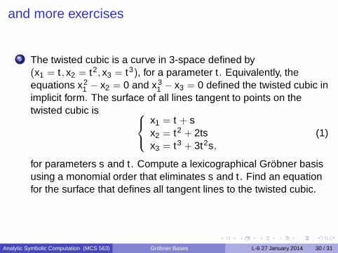
5 The twisted cubic is a curve in 3-space defined by(x1 = t , x2 = t2, x3 = t3), for a parameter t . Equivalently, theequations x2

1 − x2 = 0 and x31 − x3 = 0 defined the twisted cubic in

implicit form. The surface of all lines tangent to points on thetwisted cubic is

x1 = t + sx2 = t2 + 2tsx3 = t3 + 3t2s,

(1)

for parameters s and t . Compute a lexicographical Gröbner basisusing a monomial order that eliminates s and t . Find an equationfor the surface that defines all tangent lines to the twisted cubic.


one last exercise

6 With a lexicographical Gröbner basis and a solver for polynomialsin one variable we can solve zero dimensional polynomialsystems, systems that have only isolated solutions. Write aprocedure in a computer algebra system that takes on input alexicographical Gröbner basis and computes all solutions byapplying the univariate solver repeatedly and substituting thesolutions into the remaining equations. For a numerical solver,show that the working precision must be sufficiently high enoughas the solver progresses, considering the example of exercise 4.


Documents

Gröbner Bases - University of Illinois at Chicagohomepages.math.uic.edu/~jan/mcs563/groebner.pdf · Gröbner Bases 1 S-polynomials eliminating the leading term Buchberger’s criterion