Embed Size (px)
Citation preview
Linear Algebra and its Applications 391 (2004) 169–202www.elsevier.com/locate/laa
Applications of Gröbner bases to signal andimage processing: a survey
Zhiping Lin a,∗, Li Xu b,1, Qinghe Wu c,2
aSchool of Electrical and Electronic Engineering, Nanyang Technological University, Block S2,Nanyang Avenue, 69978 Singapore, Singapore
bDepartment of Electronics and Information Systems, Akita Prefectural University, 84-4Tsuchiya-Ebinokuchi, Honjo, Akita 015-0055, Japan
cDepartment of Automatic Control, Beijing Institute of Technology, Beijing 100081, China
Received 31 March 2003; accepted 22 January 2004
Submitted by P.C. Hansen
Abstract
This paper is a tutorial and survey paper on the Gröbner bases method and some of itsapplications in signal and image processing. Although all the results presented in the paperare available in the literature, we give an elementary treatment here, in the hope that it willfurther bring awareness of and stimulate interest in Gröbner bases among researchers in signaland image processing. We give first a tutorial on Gröbner bases, and then a survey of the designof multidimensional wavelets and filter banks. Applications of Gröbner bases to other areas ofsignal and image processing are also briefly reviewed.© 2004 Published by Elsevier Inc.
Keywords: Gröbner bases; Multidimensional filter banks; Multidimensional wavelets; FIR filter; IIR filter;Multivariate polynomial
∗ Corresponding author. Tel.: +65-6790-6857; fax: +65-6792-0415.E-mail address: [email protected] (Z. Lin).
1 Partly supported by JSPS.KAKENHI15560383.2 Currently visiting Akita Prefectural University as a research fellow. Supported by the National Nat-
ural Science Foundation of China under grant 69904003, and by the Doctoral Foundation of the EducationMinistry of China.
0024-3795/$ - see front matter � 2004 Published by Elsevier Inc.doi:10.1016/j.laa.2004.01.008
170 Z. Lin et al. / Linear Algebra and its Applications 391 (2004) 169–202
1. Introduction
The theory and algorithm of Gröbner bases were originally developed by Buch-berger in the 1960s and later on further enriched with contributions from himself andmany other researchers (see [9–13,26] and the references therein). On the one hand,the tool of Gröbner bases is no doubt one of the most powerful methods in math-ematics in general, and in algebraic geometry and commutative algebra in particular,as it is evident from the facts that numerous books and research papers on Gröb-ner bases have been published in recent years and that the Gröbner bases methodhas been implemented in all major general purpose mathematical software systemslike Mathematica, Maple, Derive, etc., see e.g. [53], and in a couple of specializedsoftware systems, notably CoCoA [16], Singular [48], and Macaulay [35]. On theother hand, Gröbner bases have also found wide applications in theoretical physics,applied science and engineering. The main reason for the success of Gröbner bases isthat many problems in mathematics, science and engineering can be represented bymultivariate polynomials (ideals, modules, matrices etc.), and Gröbner bases are wellknown to play a similar role in multivariate (nD, n > 1) polynomials as Euclideandivision algorithm in univariate (1D) polynomials. In signal and image processing,Gröbner bases have been applied to various problems in different areas, such as thedesign of multidimensional (nD) wavelets and filter banks, robust stability analysisof nD digital filters, balanced multiwavelets and digital filter design, and image pro-cessing and computer vision. In particular, for the past decade Gröbner bases havereceived noticeable attention in the design of nD wavelets and filter banks, whichcan be represented by nD polynomial and rational matrices. See, for example, therecent special issue on applications of Gröbner bases to multidimensional systemsand signal processing, guest edited by the first two co-authors of this paper [33].However, it is felt that many researchers in signal and image processing are stillunaware of the powerful tool of Gröbner bases.
The objectives of this paper are twofold, first to further bring awareness of andstimulate interest in Gröbner bases among researchers in signal and image pro-cessing, which is consistent to the purpose of this special issue, and second to surveyexisting results on applications of Gröbner bases to signal and image processing.Instead of covering the general aspects of the Gröbner bases theory and all of itsapplications in signal and image processing which would require an extensive discus-sion beyond the scope of this paper, we will be mainly concerned with the basics ofthe Gröbner bases method, and its applications to the design of nD wavelets and filterbanks. Applications of Gröbner bases to other areas of signal and image processingwill then be briefly discussed.
The organization of this paper is as follows. In the next section, we give a tu-torial on Gröbner bases. We then present a brief introduction to signal processingin Section 3 to provide some background materials and motivation for readers whoare unfamiliar with signal processing. Following that, we review existing results onthe design of nD regular nonseparable wavelets in Section 4, the design of nD finite
Z. Lin et al. / Linear Algebra and its Applications 391 (2004) 169–202 171
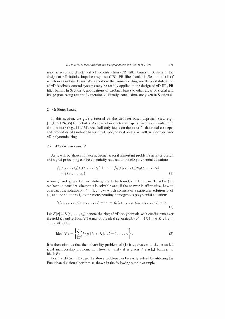
impulse response (FIR), perfect reconstruction (PR) filter banks in Section 5, thedesign of nD infinite impulse response (IIR), PR filter banks in Section 6, all ofwhich use Gröbner bases. We also show that some existing results on stabilizationof nD feedback control systems may be readily applied to the design of nD IIR, PRfilter banks. In Section 7, applications of Gröbner bases to other areas of signal andimage processing are briefly mentioned. Finally, conclusions are given in Section 8.
2. Gröbner bases
In this section, we give a tutorial on the Gröbner bases approach (see, e.g.,[11,13,21,26,36] for details). As several nice tutorial papers have been available inthe literature (e.g., [11,13]), we shall only focus on the most fundamental conceptsand properties of Gröbner bases of nD polynomial ideals as well as modules overnD polynomial ring.
2.1. Why Gröbner basis?
As it will be shown in later sections, several important problems in filter designand signal processing can be essentially reduced to the nD polynomial equation:
f1(z1, . . . , zn)x1(z1, . . . , zn)+ · · · + fm(z1, . . . , zn)xm(z1, . . . , zn)
= f (z1, . . . , zn), (1)
where f and fi are known while xi are to be found, i = 1, . . . , m. To solve (1),we have to consider whether it is solvable and, if the answer is affirmative, how toconstruct the solution xi , i = 1, . . . , m which consists of a particular solution xi of(1) and the solutions xi to the corresponding homogenous polynomial equation:
f1(z1, . . . , zn)x1(z1, . . . , zn)+ · · · + fm(z1, . . . , zn)xm(z1, . . . , zn) = 0.(2)
Let K[z]�K[z1, . . . , zn] denote the ring of nD polynomials with coefficients overthe fieldK , and let Ideal(F ) stand for the ideal generated by F = {fi | fi ∈ K[z], i =1, . . . , m}, i.e.,
Ideal(F ) ={m∑i=1
hifi |hi ∈ K[z], i = 1, . . . , m
}. (3)
It is then obvious that the solvability problem of (1) is equivalent to the so-calledideal membership problem, i.e., how to verify if a given f ∈ K[z] belongs toIdeal(F ).
For the 1D (n = 1) case, the above problem can be easily solved by utilizing theEuclidean division algorithm as shown in the following simple example.
172 Z. Lin et al. / Linear Algebra and its Applications 391 (2004) 169–202
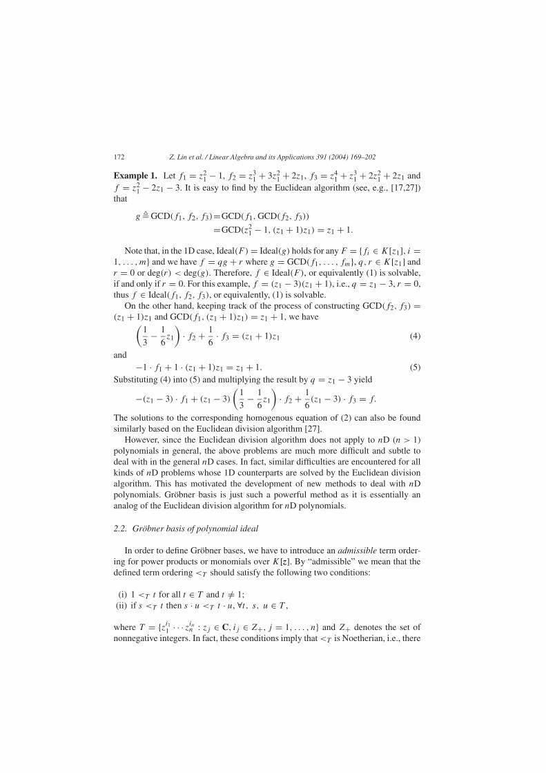
Example 1. Let f1 = z21 − 1, f2 = z3
1 + 3z21 + 2z1, f3 = z4
1 + z31 + 2z2
1 + 2z1 andf = z2
1 − 2z1 − 3. It is easy to find by the Euclidean algorithm (see, e.g., [17,27])that
g� GCD(f1, f2, f3)=GCD(f1,GCD(f2, f3))
=GCD(z21 − 1, (z1 + 1)z1) = z1 + 1.
Note that, in the 1D case, Ideal(F )= Ideal(g) holds for any F = {fi ∈ K[z1], i =1, . . . , m} and we have f = qg + r where g = GCD(f1, . . . , fm}, q, r ∈ K[z1] andr = 0 or deg(r) < deg(g). Therefore, f ∈ Ideal(F ), or equivalently (1) is solvable,if and only if r = 0. For this example, f = (z1 − 3)(z1 + 1), i.e., q = z1 − 3, r = 0,thus f ∈ Ideal(f1, f2, f3), or equivalently, (1) is solvable.
On the other hand, keeping track of the process of constructing GCD(f2, f3) =(z1 + 1)z1 and GCD(f1, (z1 + 1)z1) = z1 + 1, we have(
1
3− 1
6z1
)· f2 + 1
6· f3 = (z1 + 1)z1 (4)
and−1 · f1 + 1 · (z1 + 1)z1 = z1 + 1. (5)
Substituting (4) into (5) and multiplying the result by q = z1 − 3 yield
−(z1 − 3) · f1 + (z1 − 3)
(1
3− 1
6z1
)· f2 + 1
6(z1 − 3) · f3 = f.
The solutions to the corresponding homogenous equation of (2) can also be foundsimilarly based on the Euclidean division algorithm [27].
However, since the Euclidean division algorithm does not apply to nD (n > 1)polynomials in general, the above problems are much more difficult and subtle todeal with in the general nD cases. In fact, similar difficulties are encountered for allkinds of nD problems whose 1D counterparts are solved by the Euclidean divisionalgorithm. This has motivated the development of new methods to deal with nDpolynomials. Gröbner basis is just such a powerful method as it is essentially ananalog of the Euclidean division algorithm for nD polynomials.
2.2. Gröbner basis of polynomial ideal
In order to define Gröbner bases, we have to introduce an admissible term order-ing for power products or monomials over K[z]. By “admissible” we mean that thedefined term ordering <T should satisfy the following two conditions:
(i) 1 <T t for all t ∈ T and t /= 1;(ii) if s <T t then s · u <T t · u, ∀t, s, u ∈ T ,
where T = {zi11 · · · zinn : zj ∈ C, ij ∈ Z+, j = 1, . . . , n} and Z+ denotes the set ofnonnegative integers. In fact, these conditions imply that<T is Noetherian, i.e., there
Z. Lin et al. / Linear Algebra and its Applications 391 (2004) 169–202 173
exist no infinitely decreasing chains of the form h1 >T h2 >T · · ·, where h1 >Th2 ⇔ h2 <T h1.
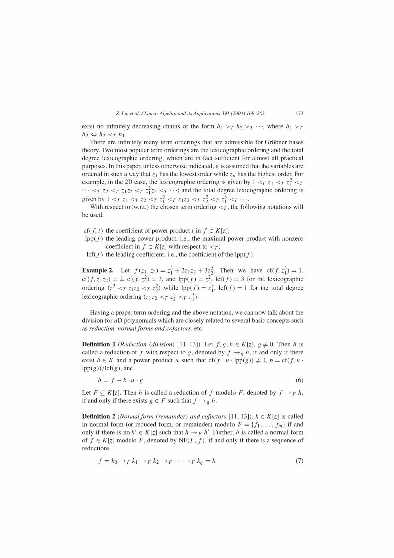
There are infinitely many term orderings that are admissible for Gröbner basestheory. Two most popular term orderings are the lexicographic ordering and the totaldegree lexicographic ordering, which are in fact sufficient for almost all practicalpurposes. In this paper, unless otherwise indicated, it is assumed that the variables areordered in such a way that z1 has the lowest order while zn has the highest order. Forexample, in the 2D case, the lexicographic ordering is given by 1 <T z1 <T z
21 <T
· · · <T z2 <T z1z2 <T z21z2 <T · · ·; and the total degree lexicographic ordering is
given by 1 <T z1 <T z2 <T z21 <T z1z2 <T z
22 <T z
31 <T · · ·.
With respect to (w.r.t.) the chosen term ordering <T , the following notations willbe used.
cf(f, t) the coefficient of power product t in f ∈ K[z];lpp(f ) the leading power product, i.e., the maximal power product with nonzero
coefficient in f ∈ K[z] with respect to <T ;lcf(f ) the leading coefficient, i.e., the coefficient of the lpp(f ).
Example 2. Let f (z1, z2) = z31 + 2z1z2 + 3z2
2. Then we have cf(f, z31) = 1,
cf(f, z1z2) = 2, cf(f, z22) = 3, and lpp(f ) = z2
2, lcf(f ) = 3 for the lexicographicordering (z3
1 <T z1z2 <T z22) while lpp(f ) = z3
1, lcf(f ) = 1 for the total degreelexicographic ordering (z1z2 <T z
22 <T z
31).
Having a proper term ordering and the above notation, we can now talk about thedivision for nD polynomials which are closely related to several basic concepts suchas reduction, normal forms and cofactors, etc.
Definition 1 (Reduction (division) [11, 13]). Let f, g, h ∈ K[z], g /= 0. Then h iscalled a reduction of f with respect to g, denoted by f →g h, if and only if thereexist b ∈ K and a power product u such that cf(f, u · lpp(g)) /= 0, b = cf(f, u ·lpp(g))/lcf(g), and
h = f − b · u · g. (6)
Let F ⊆ K[z]. Then h is called a reduction of f modulo F , denoted by f →F h,if and only if there exists g ∈ F such that f →g h.
Definition 2 (Normal form (remainder) and cofactors [11, 13]). h ∈ K[z] is calledin normal form (or reduced form, or remainder) modulo F = {f1, . . . , fm} if andonly if there is no h′ ∈ K[z] such that h→F h
′. Further, h is called a normal formof f ∈ K[z] modulo F , denoted by NF(F, f ), if and only if there is a sequence ofreductions
f = k0 →F k1 →F k2 →F · · · →F kq = h (7)
174 Z. Lin et al. / Linear Algebra and its Applications 391 (2004) 169–202
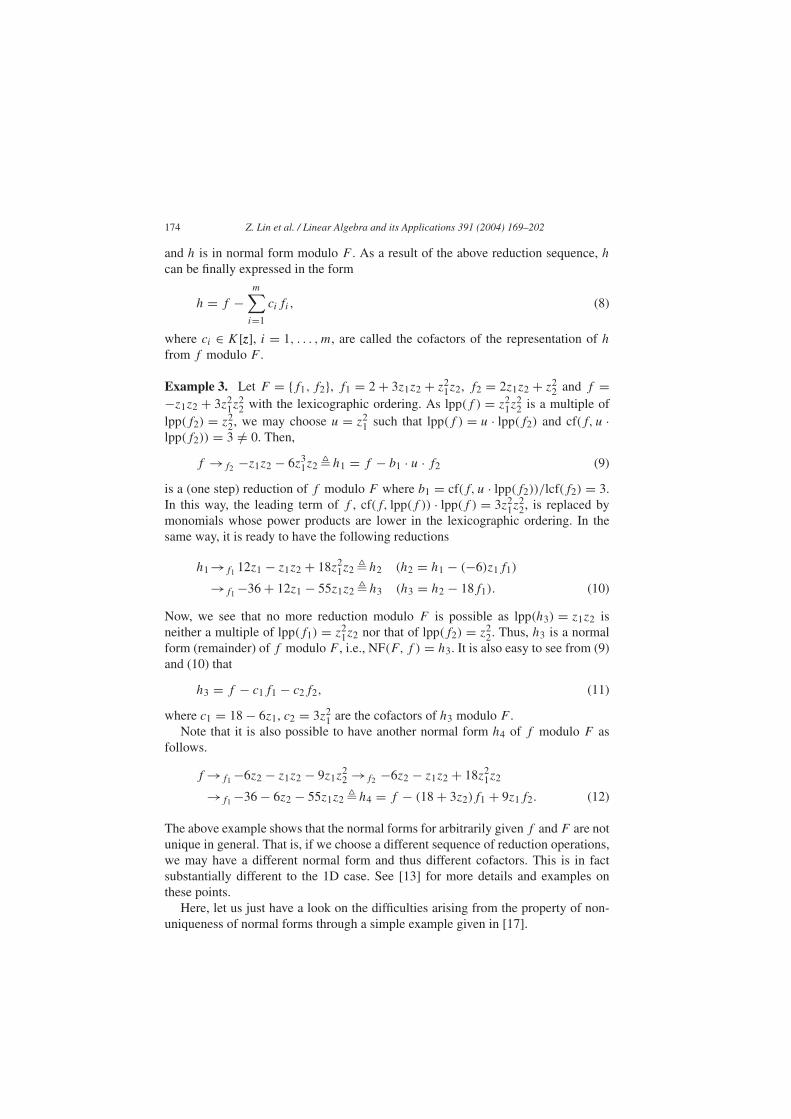
and h is in normal form modulo F . As a result of the above reduction sequence, hcan be finally expressed in the form
h = f −m∑i=1
cifi, (8)
where ci ∈ K[z], i = 1, . . . , m, are called the cofactors of the representation of hfrom f modulo F .
Example 3. Let F = {f1, f2}, f1 = 2+ 3z1z2 + z21z2, f2 = 2z1z2 + z2
2 and f =−z1z2 + 3z2
1z22 with the lexicographic ordering. As lpp(f ) = z2
1z22 is a multiple of
lpp(f2) = z22, we may choose u = z2
1 such that lpp(f ) = u · lpp(f2) and cf(f, u ·lpp(f2)) = 3 /= 0. Then,
f →f2 −z1z2 − 6z31z2 �h1 = f − b1 · u · f2 (9)
is a (one step) reduction of f modulo F where b1 = cf(f, u · lpp(f2))/lcf(f2) = 3.In this way, the leading term of f , cf(f, lpp(f )) · lpp(f ) = 3z2
1z22, is replaced by
monomials whose power products are lower in the lexicographic ordering. In thesame way, it is ready to have the following reductions
h1→f1 12z1 − z1z2 + 18z21z2 �h2 (h2 = h1 − (−6)z1f1)
→f1−36+ 12z1 − 55z1z2 �h3 (h3 = h2 − 18f1). (10)
Now, we see that no more reduction modulo F is possible as lpp(h3) = z1z2 isneither a multiple of lpp(f1) = z2
1z2 nor that of lpp(f2) = z22. Thus, h3 is a normal
form (remainder) of f modulo F , i.e., NF(F, f ) = h3. It is also easy to see from (9)and (10) that
h3 = f − c1f1 − c2f2, (11)
where c1 = 18− 6z1, c2 = 3z21 are the cofactors of h3 modulo F .
Note that it is also possible to have another normal form h4 of f modulo F asfollows.
f→f1−6z2 − z1z2 − 9z1z22 →f2 −6z2 − z1z2 + 18z2
1z2
→f1−36− 6z2 − 55z1z2 �h4 = f − (18+ 3z2)f1 + 9z1f2. (12)
The above example shows that the normal forms for arbitrarily given f and F are notunique in general. That is, if we choose a different sequence of reduction operations,we may have a different normal form and thus different cofactors. This is in factsubstantially different to the 1D case. See [13] for more details and examples onthese points.
Here, let us just have a look on the difficulties arising from the property of non-uniqueness of normal forms through a simple example given in [17].
Z. Lin et al. / Linear Algebra and its Applications 391 (2004) 169–202 175
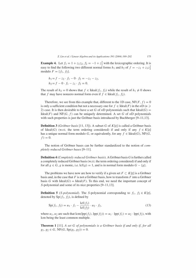
Example 4. Let f1 = 1+ z1z2, f2 = −1+ z22 with the lexicographic ordering. It is
easy to find the following two different normal forms h1 and h2 of f = −z1 + z1z22
modulo F = {f1, f2}.h1=f − z2 · f1 − 0 · f2 = −z1 − z2,
h2=f − 0 · f1 − z1 · f2 = 0.
The result of h2 = 0 shows that f ∈ Ideal(f1, f2) while the result of h1 /= 0 showsthat f may have nonzero normal form even if f ∈ Ideal(f1, f2).
Therefore, we see from this example that, different to the 1D case, NF(F, f ) = 0is only a sufficient condition but not a necessary one for f ∈ Ideal(F ) in the nD (n �2) case. It is then desirable to have a set G of nD polynomials such that Ideal(G) =Ideal(F ) and NF(G, f ) can be uniquely determined. A set G of nD polynomialswith such properties is just the Gröbner basis introduced by Buchberger [9–11,13].
Definition 3 (Gröbner basis [11, 13]). A subset G of K[z] is called a Gröbner basisof Ideal(G) (w.r.t. the term ordering considered) if and only if any f ∈ K[z]has a unique normal form modulo G, or equivalently, for any f ∈ Ideal(G), NF(G,f ) = 0.
The notion of Gröbner bases can be further standardized to the notion of com-pletely reduced Gröbner bases [9–11].
Definition 4 (Completely reduced Gröbner basis). A Gröbner basisG is further calleda completely reduced Gröbner basis (w.r.t. the term ordering considered) if and only iffor all g ∈ G, g is monic, i.e. lcf(g) = 1, and is in normal form moduloG− {g}.
The problems we have now are how to verify if a given set F ⊂ K[z] is a Gröbnerbasis and, in the case that F is not a Gröbner basis, how to transform F into a Gröbnerbasis G with Ideal(G) = Ideal(F ). To this end, we need the important concept ofS-polynomial and some of its nice properties [9–11,13].
Definition 5 (S-polynomial). The S-polynomial corresponding to f1, f2 ∈ K[z],denoted by Sp(f1, f2), is defined by
Sp(f1, f2) = u1 · f1 − lcf(f1)
lcf(f2)· u2 · f2, (13)
where u1, u2 are such that lcm(lpp(f1), lpp(f2)) = u1 · lpp(f1) = u2 · lpp(f2), withlcm being the least common multiple.
Theorem 1 [11]. A set G of polynomials is a Gröbner basis if and only if, for allg1, g2 ∈ G, NF(G, Sp(g1, g2)) = 0.
176 Z. Lin et al. / Linear Algebra and its Applications 391 (2004) 169–202
Let us now go through an example to see how the Gröbnerianity can be tested anda Gröbner basis can be constructed algorithmically based on the above property of S-polynomials. More details and examples on the algorithms and further applicationsof Gröbner basis can be found in [11,13,26].
Example 5. Let F = {f1, f2}, f1 = 2+ 3z1z2 + z21z2, f2 = 2z1z2 + z2
2 with thelexicographic ordering, as given in Example 3.
It is ready to have
Sp(f1, f2) = z2 · f1 − z21 · f2 = 2z1 − 2z3
1z2 + 3z1z22, (14)
Sp(f1, f2)→f2 2z2 − 6z21z2 − 2z3
1z2 �h (h = Sp(f1, f2)− 3z1f2)
→f1 4z1 + 2z2 = NF(F, Sp(f1, f2))
(NF(F, Sp(f1, f2)) = h− (−2)z1f1). (15)
Thus we know that F is not a Gröbner basis by Theorem 1. In fact, we have seenin Example 3 that the normal forms of f = −z1z2 + 3z2
1z22 modulo F are not unique
and thus F is not a Gröbner basis by the definition.To transform F into a Gröbner basis (see, e.g., [11,13]), adjoin (the monic version
of) NF(F, Sp(f1, f2)) f3 � 2z1 + z2 to F , and get a new set F = {f1, f2, f3}. Itis easy to see that Ideal(F ) = Ideal(F ) as f3 can be presented, due to (14) and(15), in the form f3 = c1f1 + c2f2 with c1 = z1 + z2/2 and c2 = −(3z1 + z2
1)/2.Obviously, NF(F , Sp(f1, f2)) = 0 since Sp(f1, f2) can be first reduced to NF(F,Sp(f1, f2)) = 4z1 + 2z2 as shown above and then to 0 by just subtracting 2f3.
To see if F is a Gröbner basis, we still need to check at least if NF(F ,Sp(f1, f3)) = 0. By similar calculations as above, we have
Sp(f1, f3) = f1 − z21f3 = 2− 2z3
1 + 3z1z2, (16)
NF(F , Sp(f1, f3)) = Sp(f1, f3)− 3z1f3 = 2− 6z21 − 2z3
1 /= 0, (17)
which shows that F is still not yet a Gröbner basis. Again, we can construct f4 �−1+3z2
1+z31 from NF(F , Sp(f1, f3)) and adjoin f4 to F to get F = {f1, f2, f3, f4}
which satisfies Ideal(F ) = Ideal(F ) = Ideal(F ) and NF(F , Sp(f1, f3)) = 0.It is ready to see that NF(F , Sp(f2, f3)) = 0, NF(F , Sp(f1, f4)) = 0, NF(F , Sp
(f2, f4)) = 0 and NF(F , Sp(f3, f4)) = 0. Thus, we have obtained a Gröbner basisF equivalent to F . Moreover, since f1 − (3z1 + z2
1)f3 + 2f4 = 0, f2 − z2f3 = 0,that is, the first two polynomials f1 and f2 in F can be reduced to zero with respectto f3 and f4, F is not a completely reduced Gröbner basis for F . By removing f1and f2, we then have the completely reduced Gröbner basis G� {f3, f4} equivalentto F .
After having a Gröbner basis G = {g1, . . . , gs} equivalent to F = {f1, . . . , fm},the solvability problem of (1), or the corresponding ideal membership problem, canbe solved by just testing whether or not NF(G, f ) = 0. Also, by keeping track of the
Z. Lin et al. / Linear Algebra and its Applications 391 (2004) 169–202 177
reduction processes for constructing gi ∈ G from fj ∈ F in the above constructionalgorithm of Gröbner bases, we can obtain the cofactors of gi ∈ Gmodulo F [11,13]in the form
gi =m∑j=1
cij fj , cij ∈ K[z], i = 1, . . . , s (18)
or in a slightly sloppy notation,
G = UF, U �
c11 · · · c1m...
...
cs1 · · · csm
. (19)
It is then easy to obtain a particular solution to (1) and the solutions to (2) by thereduction of f moduloG and the above relation betweenG and F . For more detailedtutorial examples, see, e.g., [13].
It should be emphasized that the uniqueness property of normal form entails alsoa lot of other important properties of Gröbner bases which play a crucial role inobtaining algorithmic solutions to numerous fundamental algebraic problems (see,e.g., [11,13]). One of the most important properties of Gröbner bases is the so-called elimination property with respect to lexicographic ordering, which provides abasis for solutions to many problems in commutative algebra such as the solution ofsystems of algebraic equations, the implicitization problem for algebraic manifolds,etc (see, e.g., [11–13]). This property is stated in the following theorem.
Theorem 2 [11, 49]. Let G be a Gröbner basis with respect to the lexicographicordering of power products. Assume without loss of generality that z1 <T · · · <T zn.Then
Ideal(G) ∩K[z1, . . . , zi] = Ideal(G ∩K[z1, . . . , zi]), i = 1, . . . , n,
(20)
where the ideal on the right-hand side is formed in K[z1, . . . , zi].
This result means that the ith elimination ideal of G is generated by just thosepolynomials in G that depend only on the variables z1, . . . , zi . For simplicity, weconsider only the case where the ideal generated by F = {f1(z), . . . , fm(z) ∈ K[z]}is of zero-dimension, i.e., the system of algebraic equations defined by fi(z) = 0,i = 1, . . . , m, has a finite number of solutions. By Theorem 2, the Gröbner basisof F with respect to the term ordering z1 <T . . . <T zn will be in the form G ={g1(z1), g2(z1, z2), . . . , gn−1(z1, . . . , zn−1), gn(z1, . . . , zn)}. Thus, due to the elim-ination property, it is possible to solve the algebraic system fi(z) = 0, i = 1, . . . , mthrough solving the corresponding algebraic system g1(z1) = 0, g2(z1, z2) = 0, . . . ,gn(z1, . . . , zn) = 0 in a “variable by variable” way. For more details and variousillustrative examples, see [11,13] and the references therein.
178 Z. Lin et al. / Linear Algebra and its Applications 391 (2004) 169–202
2.3. Gröbner basis of modules over polynomial rings
In system theory and signal processing, it is often required to solve, instead of thepolynomial equation of (1), the following polynomial matrix equation:
A(z)X(z) = C(z), (21)
where A(z) ∈ Kr×m[z] and C(z) ∈ Kr×r [z] are given, and X(z) ∈ Km×r [z] is tobe found. Let A = [a1 · · · am], X = [xij ], C = [c1 · · · cr ] with ai , cj ∈ Kr [z], i =1, . . . , m and j = 1, . . . , r . It is then obvious that (21) can be equivalently expressedas
x1ja1 + · · · + xmjam = cj , j = 1, . . . , r. (22)
Though it is possible to reduce (21) to (1) (see, e.g., [22]), it is in fact more naturaland efficient to solve (21), or equivalently (22), by applying the Gröbner basis ofmodules over an nD polynomial ring to be reviewed in this section [21,55].
Furukawa et al. [21] and Mora and Möller [36] have independently generalizedthe concept of Gröbner basis for polynomial ideal to Gröbner basis of modules overpolynomial ring, which is briefly summarized as follows [51].
Let F = {f1, . . . , fm} be a subset of Kr [z]. By Module(F ) we mean the modulegenerated by F , i.e.,
Module(F ) = {h1f1 + · · · + hmfm | hi ∈ K[z], i = 1, . . . , m}. (23)
To generalize the notion of reduction, we need first to fix an ordering on the r-tuplesof power products under certain admissible conditions. In fact we can do this byonly fixing the ordering on a subset P of r-tuples of power products which consistof tuples with only one nonzero component, i.e.,
P � {(0, . . . , 0, zi11 · · · zinn , 0, . . . , 0)T | i1, . . . , in ∈ Z+}. (24)
The elements of P are called power product tuples. Then a partial ordering <M onP is defined by
(∀p1, p2 ∈ P) [p1 <M p2 ⇔ ((∃q /= 1, q power product) p2 = q · p1)]. (25)
By an admissible ordering <M(T ) on P , we mean any total ordering which satisfiesthe following properties:
(i) (∀p1, p2 ∈ P) [p1 <M p2 ⇒ p1 <M(T ) p2].(ii) (∀p1, p2 ∈ P) [p1 <M(T ) p2 ⇒ ((∀q, q power product)q · p1 <M(T ) q · p2)].
It can be shown that every admissible ordering on P is Noetherian [51].Further, the notations �M and �M(T ) are defined as (p1 �M p2)⇔ [p1 <M p2 or
p1 = p2] and (p1 �M(T ) p2)⇔ [p1 <M(T ) p2 or p1 = p2] for all p1, p2 ∈ P .Let<T be an admissible ordering on the power products ofK[z], for example the
lexicographic ordering or the total degree (lexicographic) ordering. Let p= (0, . . . , 0,pi, 0, . . . , 0)T and q = (0, . . . , 0, qj , 0, . . . , 0)T ∈ P , where pi /= 0 occurs at the ith
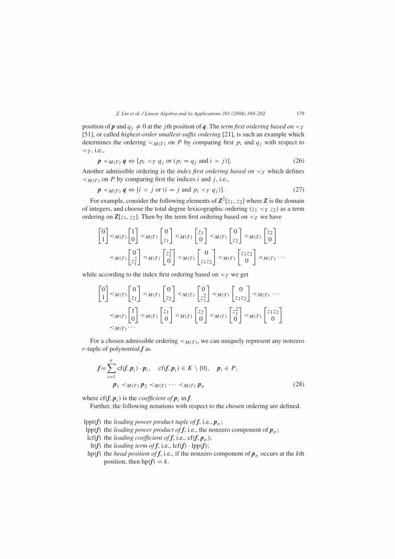
Z. Lin et al. / Linear Algebra and its Applications 391 (2004) 169–202 179
position of p and qj /= 0 at the j th position of q. The term first ordering based on<T[51], or called highest-order smallest-suffix ordering [21], is such an example whichdetermines the ordering <M(T ) on P by comparing first pi and qj with respect to<T , i.e.,
p <M(T ) q ⇔ [pi <T qj or (pi = qj and i > j)]. (26)
Another admissible ordering is the index first ordering based on <T which defines<M(T ) on P by comparing first the indices i and j , i.e.,
p <M(T ) q ⇔ [i > j or (i = j and pi <T qj )]. (27)
For example, consider the following elements of Z2[z1, z2] where Z is the domainof integers, and choose the total degree lexicographic ordering (z1 <T z2) as a termordering on Z[z1, z2]. Then by the term first ordering based on <T we have[
01
]<M(T )
[10
]<M(T )
[0z1
]<M(T )
[z10
]<M(T )
[0z2
]<M(T )
[z20
]
<M(T )
[0z2
1
]<M(T )
[z2
10
]<M(T )
[0z1z2
]<M(T )
[z1z2
0
]<M(T ) · · ·
while according to the index first ordering based on <T we get[01
]<M(T )
[0z1
]<M(T )
[0z2
]<M(T )
[0z2
1
]<M(T )
[0z1z2
]<M(T ) · · ·
<M(T )
[10
]<M(T )
[z10
]<M(T )
[z20
]<M(T )
[z2
10
]<M(T )
[z1z2
0
]<M(T ) · · ·
For a chosen admissible ordering <M(T ), we can uniquely represent any nonzeror-tuple of polynomial f as
f=σ∑i=1
cf(f, pi ) · pi , cf(f, pi ) ∈ K \ {0}, pi ∈ P,
p1 <M(T ) p2 <M(T ) · · · <M(T ) pσ (28)
where cf(f, pi ) is the coefficient of pi in f.Further, the following notations with respect to the chosen ordering are defined.
lppt(f) the leading power product tuple of f, i.e., pσ ;lpp(f) the leading power product of f, i.e., the nonzero component of pσ ;lcf(f) the leading coefficient of f, i.e., cf(f, pσ );lt(f) the leading term of f, i.e., lcf(f) · lpp(f);
hp(f) the head position of f, i.e., if the nonzero component of pσ occurs at the kthposition, then hp(f) = k.
180 Z. Lin et al. / Linear Algebra and its Applications 391 (2004) 169–202
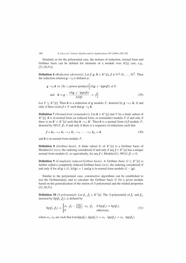
Similarly as for the polynomial case, the notions of reduction, normal form andGröbner basis can be defined for elements of a module over K[z] (see, e.g.,[21,36,51]).
Definition 6 (Reduction (division)). Let f, g, h ∈ Kr [z], f /= 0 � (0, . . . , 0)T. Thenthe reduction relation g →f is defined as
g →f h ⇔ (∃v, v power product)[cf(g, v · lppt(f)) /= 0
and h = g− cf(g, v · lppt(f))lcf(f)
· v · f]. (29)
Let F ⊆ Kr [z]. Then h is a reduction of g modulo F , denoted by g →F h, if andonly if there exists f ∈ F such that g →f h.
Definition 7 (Normal form (remainder)). Let h ∈ Kr [z] and F be a finite subset ofKr [z]. h is in normal form (or reduced form, or remainder) modulo F if and only ifthere is no h′ ∈ Kr [z] such that h →F h′. Then h is a normal form of f modulo F ,denoted by NF(F, f), if and only if there is a sequence of reductions such that
f = k0 →F k1 →F k2 →F · · · →F kq = h (30)
and h is in normal form modulo F .
Definition 8 (Gröbner basis). A finite subset G of Kr [z] is a Gröbner basis ofModule(G) (w.r.t. the ordering considered) if and only if any f ∈ Kr [z] has a uniquenormal form modulo G, or equivalently, for any f ∈ Module(G), NF(G, f) = 0.
Definition 9 (Completely reduced Gröbner basis). A Gröbner basis G ⊆ Kr [z] isfurther called a completely reduced Gröbner basis (w.r.t. the ordering considered) ifand only if for all g ∈ G, lcf(g) = 1 and g is in normal form modulo G− {g}.
Similar to the polynomial case, constructive algorithms can be established totest the Gröbnerianity and to calculate the Gröbner basis G for a given modulebased on the generalization of the notion of S-polynomial and the related properties[21,36,51].
Definition 10 (S-polynomial). Let f1, f2 ∈ Kr [z]. The S-polynomial of f1 and f2,denoted by Sp(f1, f2), is defined by
Sp(f1, f2) ={u1 · f1 − lcf(f1)
lcf(f2)· u2 · f2 if hp(f1) = hp(f2),
0 otherwise,(31)
where u1, u2 are such that lcm(lpp(f1), lpp(f2)) = u1 · lpp(f1) = u2 · lpp(f2).
Z. Lin et al. / Linear Algebra and its Applications 391 (2004) 169–202 181
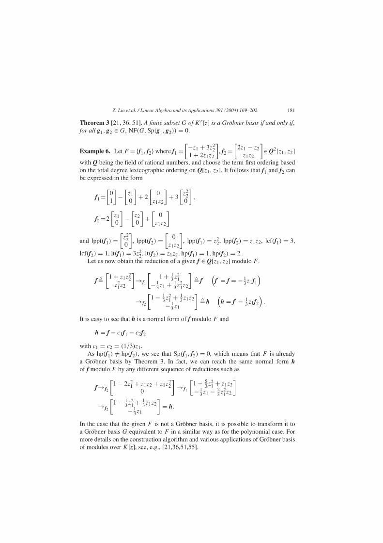
Theorem 3 [21, 36, 51]. A finite subset G of Kr [z] is a Gröbner basis if and only if,for all g1, g2 ∈ G, NF(G, Sp(g1, g2)) = 0.
Example 6. Let F = {f1, f2}where f1=[−z1 + 3z2
21+ 2z1z2
], f2=
[2z1 − z2z1z2
]∈Q2[z1, z2]
with Q being the field of rational numbers, and choose the term first ordering basedon the total degree lexicographic ordering on Q[z1, z2]. It follows that f1 and f2 canbe expressed in the form
f1=[
01
]−
[z10
]+ 2
[0z1z2
]+ 3
[z2
20
],
f2=2
[z10
]−
[z20
]+
[0z1z2
]
and lppt(f1) =[z2
20
], lppt(f2) =
[0z1z2
], lpp(f1) = z2
2, lpp(f2) = z1z2, lcf(f1) = 3,
lcf(f2) = 1, lt(f1) = 3z22, lt(f2) = z1z2, hp(f1) = 1, hp(f2) = 2.
Let us now obtain the reduction of a given f ∈ Q[z1, z2] modulo F .
f �[
1+ z1z22
z21z2
]→f1
[1+ 1
3z21
− 13z1 + 1
3z21z2
]� f′
(f′ = f = − 1
3z1f1
)
→f2
[1− 1
3z21 + 1
3z1z2
− 13z1
]� h
(h = f′ − 1
3z1f2
).
It is easy to see that h is a normal form of f modulo F and
h = f− c1f1 − c2f2
with c1 = c2 = (1/3)z1.As hp(f1) /= hp(f2), we see that Sp(f1, f2) = 0, which means that F is already
a Gröbner basis by Theorem 3. In fact, we can reach the same normal form hof f modulo F by any different sequence of reductions such as
f→f2
[1− 2z2
1 + z1z2 + z1z22
0
]→f1
[1− 5
3z21 + z1z2
− 13z1 − 2
3z21z2
]
→f2
[1− 1
3z21 + 1
3z1z2
− 13z1
]= h.
In the case that the given F is not a Gröbner basis, it is possible to transform it toa Gröbner basis G equivalent to F in a similar way as for the polynomial case. Formore details on the construction algorithm and various applications of Gröbner basisof modules over K[z], see, e.g., [21,36,51,55].
182 Z. Lin et al. / Linear Algebra and its Applications 391 (2004) 169–202
3. Introduction to signal processing
In this section, we give a brief introduction to some fundamental concepts insignal processing. This is to prepare the background for the review of applicationsof Gröbner bases to multidimensional wavelets and filter banks to be presented inthe subsequent sections. Our presentation follows [50] closely. For simplicity ofexposition, we consider only one-dimensional (1D) signal processing in this section.Most concepts could be easily generalized to the multidimensional (nD) case.
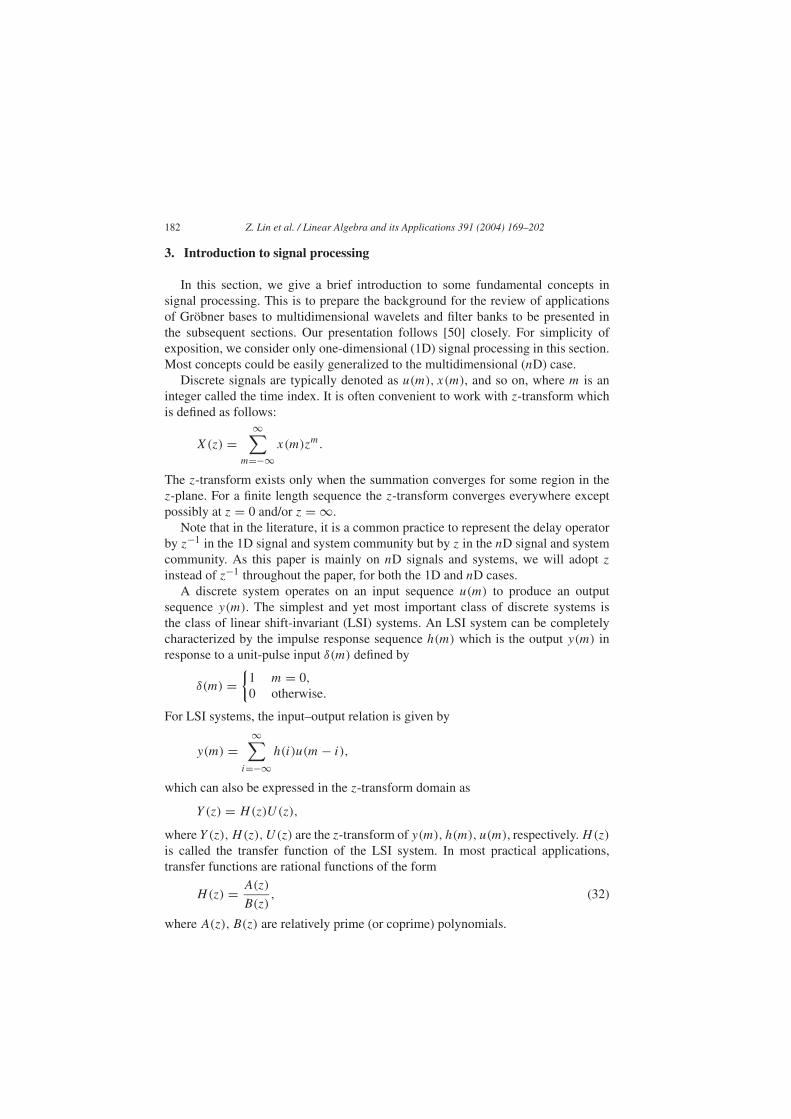
Discrete signals are typically denoted as u(m), x(m), and so on, where m is aninteger called the time index. It is often convenient to work with z-transform whichis defined as follows:
X(z) =∞∑
m=−∞x(m)zm.
The z-transform exists only when the summation converges for some region in thez-plane. For a finite length sequence the z-transform converges everywhere exceptpossibly at z = 0 and/or z = ∞.
Note that in the literature, it is a common practice to represent the delay operatorby z−1 in the 1D signal and system community but by z in the nD signal and systemcommunity. As this paper is mainly on nD signals and systems, we will adopt zinstead of z−1 throughout the paper, for both the 1D and nD cases.
A discrete system operates on an input sequence u(m) to produce an outputsequence y(m). The simplest and yet most important class of discrete systems isthe class of linear shift-invariant (LSI) systems. An LSI system can be completelycharacterized by the impulse response sequence h(m) which is the output y(m) inresponse to a unit-pulse input δ(m) defined by
δ(m) ={
1 m = 0,0 otherwise.
For LSI systems, the input–output relation is given by
y(m) =∞∑
i=−∞h(i)u(m− i),
which can also be expressed in the z-transform domain as
Y (z) = H(z)U(z),where Y (z),H(z), U(z) are the z-transform of y(m), h(m), u(m), respectively.H(z)is called the transfer function of the LSI system. In most practical applications,transfer functions are rational functions of the form
H(z) = A(z)
B(z), (32)
where A(z), B(z) are relatively prime (or coprime) polynomials.
Z. Lin et al. / Linear Algebra and its Applications 391 (2004) 169–202 183
A discrete system is said to be causal if the output y(m) at timem does not dependon the future values of the input sequence, i.e., does not depend on u(i), i > m. AnLSI system is causal if and only if the impulse response h(m) = 0 for m < 0. AnLSI system is stable if and only if
∑∞m=−∞ |h(m)| <∞. The stability condition can
also be conveniently expressed in terms of H(z), that is, an LSI system is stable ifand only if H(z) has no poles in the closed unit disc U � {z ∈ C : |z| � 1}, whereC is the field of complex numbers. This condition is equivalent to that B(z) has nozeros in U . In such a case, we also call B(z) a stable polynomial.
A finite impulse response (FIR) system is one for which B(z) = 1 in (32).A causal N th order FIR filter can be represented as
H(z) =N∑m=0
h(m)zm, h(N) /= 0. (33)
Obviously, FIR systems are inherently stable. An LSI system which is not FIR issaid to be an infinite impulse response (IIR) system.
Corresponding to the transfer function H(z), the quantity H(ejω) is called fre-quency response where the real variable ω stands for frequency. The frequencyresponse, which in general is a complex quantity, can be expressed as
H(ejω) = |H(ejω)|ejφ(ω). (34)
The real-valued quantities |H(ejω)| and φ(ω) are called the magnitude response andthe phase response of the filter, respectively.
A digital filter is said to have linear phase (LP) if the phase response φ(ω) islinear in ω. However, in the signal and image processing community, a less stringentdefinition for LP is often adopted, which is given as
H(ejω) = ce−jKωHR(ω), (35)
where c is a possibly complex constant, j = √−1, K is real, and HR(ω) is a realvalued function of ω. According to this definition, a real coefficient FIR filterH(z) =∑Nm=0 h(m)z
m is LP if and only if h(m) = h(N −m) or h(m) = −h(N −m), form = 0, 1, . . . , N . In some applications such as image and video signal processing,the LP property is very important.
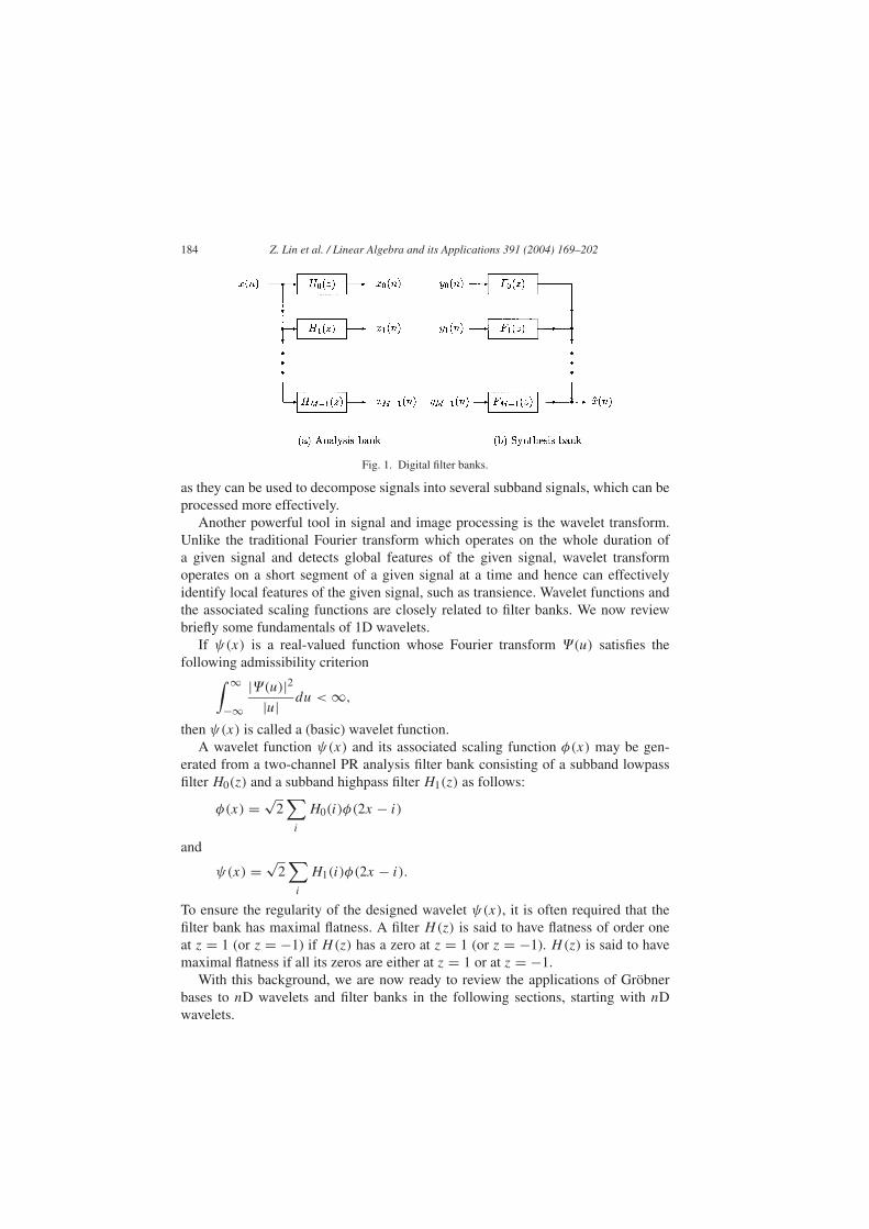
A digital filter bank is a collection of digital filters, with a common input or acommon output. Both of these cases are shown in Fig. 1. The system in Fig. 1(a)is called an analysis bank while the system in Fig. 1(b) is called a synthesis bank.Suppose that the filter bank consists of Q filters, we say that the filter bank is a Q-channel (or Q-band) filter bank and the individual filters are called subband filters.Usually each filter in a filter bank covers only a certain band of frequencies in thespectrum and hence the usage of “subband filter” is justified. A discrete systemconsisting of the cascade of an analysis filter bank and a synthesis filter bank is saidto have the perfect reconstruction (PR) property if its output and input signals areidentical except possibly for delay. In such a case, we have a PR analysis filter bankand a PR synthesis filter bank. Filter banks are very useful in a variety of applications
184 Z. Lin et al. / Linear Algebra and its Applications 391 (2004) 169–202
Fig. 1. Digital filter banks.
as they can be used to decompose signals into several subband signals, which can beprocessed more effectively.
Another powerful tool in signal and image processing is the wavelet transform.Unlike the traditional Fourier transform which operates on the whole duration ofa given signal and detects global features of the given signal, wavelet transformoperates on a short segment of a given signal at a time and hence can effectivelyidentify local features of the given signal, such as transience. Wavelet functions andthe associated scaling functions are closely related to filter banks. We now reviewbriefly some fundamentals of 1D wavelets.
If ψ(x) is a real-valued function whose Fourier transform �(u) satisfies thefollowing admissibility criterion∫ ∞
−∞|�(u)|2|u| du <∞,
then ψ(x) is called a (basic) wavelet function.A wavelet function ψ(x) and its associated scaling function φ(x) may be gen-
erated from a two-channel PR analysis filter bank consisting of a subband lowpassfilter H0(z) and a subband highpass filter H1(z) as follows:
φ(x) = √2∑i
H0(i)φ(2x − i)
and
ψ(x) = √2∑i
H1(i)φ(2x − i).
To ensure the regularity of the designed wavelet ψ(x), it is often required that thefilter bank has maximal flatness. A filter H(z) is said to have flatness of order oneat z = 1 (or z = −1) if H(z) has a zero at z = 1 (or z = −1). H(z) is said to havemaximal flatness if all its zeros are either at z = 1 or at z = −1.
With this background, we are now ready to review the applications of Gröbnerbases to nD wavelets and filter banks in the following sections, starting with nDwavelets.
Z. Lin et al. / Linear Algebra and its Applications 391 (2004) 169–202 185
4. Regular nonseparable multidimensional wavelets
Although 1D wavelets have been extensively investigated in the past decades,much less attention has been directed to nD wavelets due to the increasing com-plexity in dealing with the latter. On the other hand, image and video signals arenD in nature and the common practice in dealing with these nD signals is to exploitseparable nD wavelets, i.e., wavelets which are products of 1D wavelets. It is knownthat separable wavelets are in general only suboptimal and hence it is desirable tohave nD nonseparable wavelets.
In this section, we review a method for the design of regular nonseparable two-dimensional (2D) wavelets using Gröbner bases techniques presented in [20]. Con-sider a four-channel 2D PR analysis filter bank consisting of four 2D FIR filtersH0(z1, z2), . . . , H3(z1, z2). Wavelets may be generated from the above filter bankusing the following equations:
φ(x, y) =∑i,j
φ(2x − i, 2y − j)H0(i, j), (36)
ψ1(x, y) =∑i,j
φ(2x − i, 2y − j)H1(i, j), (37)
ψ2(x, y) =∑i,j
φ(2x − i, 2y − j)H2(i, j), (38)
ψ3(x, y) =∑i,j
φ(2x − i, 2y − j)H3(i, j), (39)
where φ is the scaling function and ψ1, ψ2, ψ3 are the wavelets. To ensure maximalflatness (regularity) of the designed wavelets, some additional conditions have to beimposed. There are several ways to design regular nonseparable 2D PR filter banks,such as numerical optimization, cascade form [25] and state-space representation. Itturns out that the cascade form approach directly leads to the application of Gröbnerbases, as presented in [20] and reviewed in the following. Note that an additionaladvantage of the cascade form is that linear phase is guaranteed.
Let
Ri =
cosαi − sinαi 0 0sinαi cosαi 0 0
0 0 cosβi − sinβi0 0 sinβi cosβi
, W = 1√
2
1 0 1 00 1 0 11 0 −1 00 1 0 −1
,
P =
1 0 0 00 1 0 00 0 0 10 0 1 0
, D(z1, z2) =
1 0 0 00 z1 0 00 0 z2 00 0 0 z1z2
,
186 Z. Lin et al. / Linear Algebra and its Applications 391 (2004) 169–202
H(z1, z2) = R1WP
K∏i=2
D(z1, z2)PWRiWP, (40)
where 2K × 2K is the size of support for the filters. The cascade form for the familyof nonseparable 2D PR linear phase filter banks is then given by (with the samplingmatrix equal to 2I )
Hi(z1, z2)=Hi,0(z21, z
22)+Hi,1(z
21, z
22)z1 +Hi,2(z
21, z
22)z2
+Hi,3(z21, z
22)z1z2, i = 0, . . . , 3 (41)
where Hi,j denotes the i, j component of the matrix H. To ensure that the filtersH0, . . . , H3 are maximally flat, i.e., with flatness of order N at given points, thefollowing conditions have to be satisfied for all k1, k2, k1 + k2 < N (Note: < wasmistaken as � in [20])
(∂k1+k2H0)/∂zk11 ∂z
k22 vanishes at (1,−1), (−1,−1), (−1, 1);
(∂k1+k2H1)/∂zk11 ∂z
k22 vanishes at (1,−1), (1, 1), (−1, 1);
(∂k1+k2H2)/∂zk11 ∂z
k22 vanishes at (1, 1), (−1,−1), (−1, 1);
(∂k1+k2H3)/∂zk11 ∂z
k22 vanishes at (1,−1), (−1,−1), (1, 1).
Note that the above flatness equations are polynomial equations with respect tocosαi, sinαi , cosβi, sinβi , and hence, together with the extra equations of sin2 γ +cos2 γ = 1 (γ = αi, βi), can be solved by using the Gröbner basis algorithm. Forexample, when N = 2 and K = 3, there are six angles and hence 12 variables in thepolynomial system. For eachHi (i = 0, . . . , 3),Hi = 0, �Hi/�z1 = 0, �Hi/�z2 = 0at three points will make 36 equations. Considering the six extra equations imposingsin2+ cos2 = 1, there will be 40 equations in the polynomial system altogether. Itturns out that this polynomial system is a zero-dimensional one and hence thereis a unique solution to the system. Although the same wavelet coefficients wereproduced in [20,25], the Gröbner basis algorithm adopted in [20] is much simplercomputationally compared with the direct method reported in [25].
When N and/or K increase, the number of equations in the polynomial systemincreases drastically and it is hence very important to develop symbolic computationsoftware package that is able to solve polynomial system with a large number ofequations. A novel method was proposed in [20] which was able to design 2Dnonseparable PR linear phase FIR filter banks for N up to 5 and K up to 8 bycombining the method of substitution of variables with Gröbner bases tools. Thedetailed discussion on this method is rather involved and the reader is referred to[20] for more details. The above method could also be extended to the design of reg-ular nonseparable higher-dimensional wavelets, although the number of polynomialequations would increase significantly.
Z. Lin et al. / Linear Algebra and its Applications 391 (2004) 169–202 187
5. Multidimensional FIR filter banks
One of the main applications of Gröbner bases to signal and image processing isthe design of multidimensional FIR perfect reconstruction filter banks. We requiresome notation and background adopted from [14,50].
For a vector p = (p1, . . . , pn)T, and a matrix M = [m1 · · ·mn] composed of
vectors mi , i = 1, . . . , n, define zp �∏ni=1 z
pii , and zM � (zm1 , . . . , zmn).
In an nD multirate system, the decimation (sampling) matrix is an n× n nonsin-gular integer matrix and the number of bandsm is equal to | detM|. There are exactlym distinct cosets for M . Select one vector from one coset, and these m vectors arecalled coset vectors. The sampled version of an nD signal xa(k) is given by
x(k) = xa(Mk),
where k is an integer vector. The set of all sample points, t = Mk, is called the latticegenerated by the matrix M , denoted by LAT(M).
In filter bank analysis and design, it is often convenient to use polyphase decom-position.
Definition 11 [14]. A polynomial a(z) is self-(anti)symmetric with index n, denotedby Ind(a) = n, if it satisfies a(z) = ±zna(z−1); a pair of polynomials a(z) and b(z)are cross-(anti)symmetric with index m, if they satisfy a(z) = ±zmb(z−1).
Definition 12 [14]. The kth subband filter Hk(z) of the m-channel filter bank is oftype ki if its index nk can be represented as nk = Mmk + ki , where ki is an integervector in LAT (M).
LetA represent an analysis polyphase matrix whose (k, l)-elementHkl is obtainedfrom
Hk(z) =m−1∑l=0
zklHkl(zM), (42)
where Hk(z) is the kth analysis subband filter.Similarly, let B represent a synthesis polyphase matrix whose (l, k)-element Flk
is obtained from
Fk(z) =m−1∑l=0
zkl Flk(zM), (43)
where Fk(z) is the kth synthesis subband filter.Perfect reconstruction (PR) is achieved if B(z)A(z) = zsI for some integer vector
s. A special case is the delay free case whenB(z)A(z) = I . For an nD PR FIR systemconsisting of an analysis filter bank and a synthesis filter bank, the output signal ofthis PR FIR system will be the same as the input system except for some possibledelays. In the case of delay free, the output signal will be identical to the input signal.
188 Z. Lin et al. / Linear Algebra and its Applications 391 (2004) 169–202
Note that the polyphase matricesA(z) and B(z) are in general Laurent polynomialmatrices whose elements are Laurent polynomials, i.e., polynomials in the variablesz1, . . . , zn, z
−11 , . . . , z−1
n . Using a technique proposed by Park et al. [40] for convert-ing a Laurent polynomial into a polynomial, we can assume that A(z) and B(z) arejust polynomial matrices for convenience of exposition.
Consider a Q-channel nD FIR filter bank. When Q = m where m = | detM|,withM being the sampling matrix, it becomes the maximally decimated (or criticallysampled) filter bank. When Q < m, it is clear that PR cannot be achieved. On theother hand, ifQ > m, the so-called nonmaximally decimated (or oversampled) filterbank case, there are infinite number of synthesis polyphase matrices B(z) satisfy-ing the PR condition for a given analysis polyphase matrix A(z) that is zero rightprime (see [32,37,56] for more details regarding factorizations and primeness fornD polynomial matrices), i.e., A(z) is of full rank for all z ∈ Cn.
With this background, we are now ready to give a survey of results on FIR, PRfilter bank design using Gröbner bases.
5.1. Analysis filters in nD FIR, PR filter banks
One of the important questions in the design of analysis filters in 1D and nDfilter banks is that given one or more analysis subband filters, how to constructthe remaining analysis subband filters such that the resultant filter bank satisfies thePR condition, or mathematically, the resultant polyphase matrix is unimodular, i.e.,matrix whose determinant is a nonzero constant. This problem has been well studiedin the 1D context [50] because the classical Euclidean division algorithm can bereadily applied here. In the nD setting, the situation is more complicated. Although azero right prime nD polynomial matrix can always be completed into a unimodularmatrix, current construction algorithms for this purpose are still fairly complicatedand inefficient [29,39]. A heuristic yet more efficient algorithm for nD unimodularmatrix completion was proposed in [38] and its improved version has recently beenproposed in [14], based on new results on nD polynomial matrix factorizations [8,31]and Gröbner bases.
The problem of constructing an nD FIR filter bank with both the PR and LPproperties becomes more difficult and remains open except for some special cases.In the following, we review a recent result on the construction of two-channel nDFIR, LP, PR filter banks [14].
Fact 1 [14]. Consider the two-channel (m = 2) case, i.e., the polyphase matrixH(z)is given by
H(z) =[H00(z) H01(z)H10(z) H11(z)
], (44)
whereH00(z) andH01(z) are the polyphase components of the specified FIR, LP, PRsubband filter H0(z) while H10(z) and H11(z) will be the polyphase components of
Z. Lin et al. / Linear Algebra and its Applications 391 (2004) 169–202 189
the other FIR subband filter H1(z). Assume that H00(z) and H01(z) do not have anynontrivial common zeros, then it is possible to constructH10(z) andH11(z) such thatH1(z) is LP and the resultant filter bank is PR, i.e., detH(z) = 1. The constructionof H10(z) and H11(z) can be carried out via the following four steps.
1. Compute the Gröbner basis of the ideal generated by H00(z) and H01(z).2. Trace back the Gröbner basis computation to obtain H ′10(z) and H ′11(z) such that
H00(z)H ′10(z)−H01(z)H ′11(z) = zs, (45)
where s = (m01 +m10)/2 and mij is an index of the self-(anti)symmetric filterHij (z). m00 and m11 are chosen such that m00 +m11 = m01 +m10 and s is aninteger vector.
3. Let H′′10(z)� zm10H ′10(z
−1), H′′11(z)� zm11H ′11(z
−1).
4. Let
H10(z) = 1
2
[H ′10(z)+H
′′10(z)
], H11(z) = 1
2
[H ′11(z)+H
′′11(z)
]. (46)
H10(z) and H11(z) will then be the polyphase components of the desired FIR,LP, PR filter corresponding to H00(z) and H01(z).
A nontrivial design example is also provided in [14] for a two-channel 2D LP, PRfilter bank, where the 2D low-pass filter is generated using McClellan transformation.The reader is referred to [14] for more details.
While the design of two-channel nD FIR, LP, PR analysis filter banks is solved,the design for the general m-channel (m > 2) nD FIR LP, PR filter banks remainsas an open problem at present [14].
5.2. Synthesis filters in nD FIR, PR filter banks
The design of synthesis filters in nD PR filter banks arises from both the max-imally decimated [43] and the nonmaximally decimated [41] filter bank cases. Ineither case, the objective is to design the corresponding synthesis filter bank givenan analysis nD filter bank subject to the PR condition. Mathematically, the designof synthesis nD filter banks can be formulated as the following problem:
Consider an nD polynomial matrix A(z) ∈ RQ×J [z], with Q � J , find anothernD polynomial matrix B(z) ∈ RJ×Q[z] such that
B(z)A(z) = I. (47)
B(z) is also called the left inverse of A(z). A necessary and sufficient condition forthe existence of B(z) is that A(z) is zero right prime. The case of Q = J is trivialhere since A(z) being zero right prime means that detA(z) is a nonzero constant.Hence B(z) = A−1(z) ∈ RJ×Q[z]. Consider now the case of Q < J .
190 Z. Lin et al. / Linear Algebra and its Applications 391 (2004) 169–202
There are several methods for solving (47) (see [2,40,44,55,56]). As Gröbnerbasis algorithm is constructive and efficient, we review here two methods that useGröbner bases to solve (47) in the design of synthesis nD FIR, PR filter banks.
Fact 2 [44]. LetA(z) ∈ RQ×J [z],withQ > J.Assume thatA(z) is zero right prime.Then the left inverse B(z) of A(z) can be obtained constructively by the followingfive steps:
1. Compute all the J × J minors of A, denoted by e1, . . . , eβ .
2. Compute the reduced Gröbner basisG for the ideal generated by e1, . . . , eβ . SinceA(z) is zero right prime by assumption, G = {1}.
3. Trace back the Gröbner basis computation to obtain λ1, . . . , λβ, such that∑β
i=1 λiei = 1.4. For i = 1, . . . , β, construct polynomial matrix Bi from A such that BiA = eiI .5. Let B =∑β
i=1 λiBi. It is then easy to verify that BA =∑β
i=1 λiBiA =∑β
i=1 λieiI = I. Therefore, B(z) is the required left inverse of A(z).
Fact 3 [40]. LetA(z) ∈ RQ×J [z],withQ > J.Assume thatA(z) is zero right prime.Then the left inverse B(z) of A(z) can be obtained constructively by the followingthree steps:
1. Compute the reduced GröbnerG basis for the module generated by all the rows ofA, i.e., a1, . . . , aQ. Since A(z) is zero right prime by assumption, G ={e1, . . . , eJ }, where e1, . . . , eJ are the standard basis row vectors.
2. Trace back the Gröbner basis computation to obtain
e1...
eJ
=
b11 . . . b1Q...
. . ....
bJ1 . . . bJQ
a1...
aQ
or
I = BA.Therefore, B(z) is the required left inverse of A(z).
Once the polyphase matrix B(z) is obtained, the synthesis filter bank can becalculated according to Eq. (43).
Remark 1. When J = 1, Facts 2 and 3 are the same. When J > 1, Fact 3 is in gen-eral more efficient to implement than Fact 2, as the number of minors of a rectangularmatrix increases drastically when the size of the matrix increases moderately [30].
Remark 2. Facts 2 and 3 were actually proposed by researchers in systems andcontrol much earlier (see [7,55] respectively). The relationship between signal and
Z. Lin et al. / Linear Algebra and its Applications 391 (2004) 169–202 191
image processing and systems and control will be further explored when we discussnD IIR filter bank design.
So far we have only discussed the computation of one left inverse of A(z), or thedesign of one synthesis filter bank. Clearly, when Q > J , there are infinite numberof such synthesis filter banks for the given analysis filter bank represented by A(z).The parameterization of the class of all such synthesis filter banks was in fact doneby Park [41,43] using Gröbner bases again and reviewed as follows.
Fact 4 [41, 43]. Consider A(z) ∈ RQ×J [z], with Q > J. Assume that A(z) is zeroright prime. Then the set of all left inverses B(z) of A(z) can be parameterized asfollows:
1. Compute a particular left inverse Bpart using Fact 2 or Fact 3.2. Compute the reduced Gröbner basis G = {g1, . . . , gl} for the syzygy module ofA, i.e. Syz(A), where gi (i = 1, . . . , l) are row vectors. Let
Gmat �
g1...
gl
∈ Rl×Q[z].
3. The parameterization of the class of all such synthesis filter banks is then givenby B = Bpart + UGmat, where U ∈ RJ×l[z] is arbitrary.
The parameterization of all the synthesis filter banks is very useful in the designof optimal synthesis nD FIR, PR filter bank as we are now able to optimize the filtercoefficients of U freely while satisfying the PR condition. Details on the optimaldesign of nD synthesis filter banks and also a design example can be found in [43].
In image and video processing, other than the PR condition, linear phase (LP) forthe filter banks is often required as well. While it is not easy to give a closed-formexpression for the parameterization of all the synthesis filter banks satisfying bothPR and LP conditions, it is possible to impose linear phase or zero phase conditionduring the design stage [43].
5.3. Two-dimensional FIR lossless systems
A square Laurent polynomial matrix H(z) is called paraunitary if it satisfiesHH = HH = I , where H (z1, . . . , zn)�H(z−1
1 , . . . , z−1n )
T. Two-dimensional (2D)FIR lossless systems are characterized by 2D paraunitary matrices, that is, a 2D FIRsystem is lossless if its transfer matrix is a 2D paraunitary matrix. Note that the filterbanks associated with paraunitary matrices are both FIR and have the PR property.However, the converse is in general not true.
As for 1D systems, 2D paraunitary matrices play an important role in 2D nonsep-arable FIR filter bank design, lossless FIR filter bank realization and other related
192 Z. Lin et al. / Linear Algebra and its Applications 391 (2004) 169–202
areas. It is straightforward to characterize 2D FIR paraunitary matrices which arefactorable into rotations and delays. A challenging problem was whether there exis-ted 2D paraunitary matrices that were not factorable into rotations and delays, i.e., 2Dnonfactorable paraunitary matrices. Recently, using Gröbner bases, Park has shown[42] that the lowest total degree of a 2D FIR nonfactorable paraunitary matrix is 4and of type (2, 2) (the total degree and type of a 2D FIR paraunitary matrix will bedefined shortly). Furthermore, he also gave a closed-form expression for the class of2D 2× 2 nonfactorable paraunitary matrices. We now give a review of the results on2D FIR paraunitary matrices presented in [42], with an emphasis on the applicationof Gröbner bases.
For simplicity of discussion, only 2D paraunitary polynomial matrices are con-sidered since 2D paraunitary Laurent matrices can be easily converted to the former.A 2D polynomial matrix H(z1, z2) =∑k1
i=0
∑k2j=0Hij z
i1zj
2 is said to be of type(k1, k2) and of total degree k= k1+k2, whereHij are constant matrices withHk1k2 /=0 [42].
Let H(z1, z2) be a 2× 2 paraunitary polynomial matrix, and let v(z1, z2) be itsfirst column vector. It was shown in [42] that the factorability of H is equivalent tothat of v. When v is of type (2, 0) and of type (0, 2), v is always factorable since theseare just the 1D cases. If v is of type (1, 1), it can be expressed as
v = v00 + v10z1 + v01z2 + v11z1z2 (48)
for some constant real vectors v00, v10, v01, v11. Let vij =[aijbij
], where aij , bij are
real numbers to be determined. Define the five polynomials hi (i = 1, . . . , 5) in thepolynomial ring
R[a00, a10, a01, a11, b00, b10, b01, b11]by
h1=a01a10 + b01b10, (49)
h2=a00a11 + b00b11, (50)
h3=a00a10 + a01a11 + b00b10 + b01b11, (51)
h4=a00a01 + a10a11 + b00b01 + b10b11, (52)
h5=a200 + a2
01 + a210 + a2
11 + b200 + b2
01 + b210 + b2
11 − 1. (53)
It can be easily shown [42] by setting vv = 1 that the set of common real zeros of thepolynomials hi’s, or equivalently the variety of the ideal generated by hi’s denoted byV (h1, . . . , h5), completely characterizes v of type (1, 1). Next, it was shown in [42]that v, and hence Hij , of type (1, 1) is factorable for all the aij , bij that are the realzeros of the polynomial h� (a00b01 − b00a01)(a00b10 − b00a10), or equivalently arein V (h). Therefore, the problem of determining the factorability ofHij of type (1, 1)is equivalent to testing whether
V (h1, . . . , h5) ⊂ V (h)? (54)
Z. Lin et al. / Linear Algebra and its Applications 391 (2004) 169–202 193
This is in fact the determination of the radical membership problem. Using Gröb-ner bases, Park showed [42] that the above question indeed has a positive answerand hence, all 2× 2 paraunitary polynomial matrices of type (1, 1) are factorable.Therefore, all 2× 2 2D FIR paraunitary polynomial matrices of total degree 2 arefactorable. Using Gröbner bases, Park then went on to show that all 2× 2 2D FIRparaunitary polynomial matrices of total degree 3 are also factorable. For 2× 2 2DFIR paraunitary polynomial matrices of total degree 4, those of types (3, 1) and(1, 3) are factorable, while there exist 2× 2 nonfactorable paraunitary polynomialmatrices of type (2, 2). In fact, although the nonfactorability conditions for this casewere formulated into a system of nD polynomial equations, which could be solved inprinciple using Gröbner bases, the solution became too complicated for the currentlyavailable software that implements Gröbner bases computation. The problem wasthen resolved by using a convex geometric approach instead. This reinforces thefact that while Gröbner bases are very powerful in solving problems involving nDpolynomials, much is still needed to improve software packages implementing thecomputation of Gröbner bases. For more details on the parameterization of 2D FIRlossless systems, see [42].
Remark 3. Before ending this section, it is worth emphasizing the advantages ofusing Gröbner bases for the analysis and design of nD FIR filter banks. Althoughthere exist other methods for this topic (see, e.g., [1,50]), one of the advantagesof adopting Gröbner bases over other methods is that the Gröbner bases method isa systematic and effective approach in dealing with nD filter banks which can berepresented by nD polynomial matrices. Another advantage of using the Gröbnerbases method is that it can often give a parameterization of all the solutions whenthey exist [41,43].
6. Multidimensional IIR filter banks
In comparison with nD FIR, PR filter banks, relatively less attention has beenpaid to nD IIR, PR filter banks, both in the 1D and nD cases. This is not because IIRfilter banks are not as useful as FIR filters. In fact, IIR filter banks are well knownto have superior frequency behavior at low computational cost [3]. However, dueto the inherent stability problem and structure complexity associated with rationalfunctions (matrices), IIR, PR filter banks are more difficult to analyze and design thanFIR filter banks. This is particularly so for the nD case. Despite of these difficulties,some progress has been made in the design of nD causal, stable PR IIR filter banksin recent years. In the following, we review results on the design of IIR filter banksusing Gröbner bases, and also present some new results by exploiting existing resultsin nD feedback control system design developed by us in recent years. We will bemainly concerned with this problem: Given a specific analysis 2D stable IIR filter,
194 Z. Lin et al. / Linear Algebra and its Applications 391 (2004) 169–202
design the remaining analysis filters such that the resultant filter bank is PR. As thegeneral nD (n > 2) case is more difficult and several problems are still outstanding,we begin our discussion with 2D IIR filter banks.
6.1. Two-dimensional IIR, PR filter banks
Similar to the discussion on FIR filter banks, we first review some properties andresults on stable nD/2D rational matrices, which are associated with nD/2D IIR filterbanks in the same way as nD/2D polynomials matrices with nD/2D FIR filter banks.
Let f (z) ∈ R[z]. f (z) is said to be a stable polynomial if f (z) has no zeros inthe closed unit polydisc U
n� {z ∈ Cn : |z1| � 1, |z2| � 1, . . . , |zn| � 1}. A rationalfunction p(z)/d(z), with p(z), d(z) being factor coprime polynomials, i.e., they donot have any nontrivial common factors [4–6,19], is said to be stable if d(z) is astable polynomial. We denote the ring of all stable rational functions by Rs(z).
Fact 5. Let f1(z1, z2), . . . , fQ(z1, z2) ∈ Rs(z1, z2) be factor coprime. If f1(z1, z2),
. . . , fQ(z1, z2) have no common zeros in U2, then there exist x1(z1, z2), . . . ,
xQ(z1, z2) ∈ Rs(z1, z2) such that
f1(z1, z2)x1(z1, z2)+ · · · + fQ(z1, z2)xQ(z1, z2) = 1, (55)
which can be constructively obtained by using the Gröbner bases approach.
Several methods have been proposed for solving Eq. (55). It was shown in [23,55]that Gröbner bases are an attractive and efficient method. The key step in all themethods for the solution to Eq. (55) is the construction of a 2D stable polynomials(z1, z2) that vanishes in the variety of the ideal generated by fi (z1, z2)’s. This isalways possible since for factor coprime rational functions fi (z1, z2)’s, the varietyof the ideal generated by fi (z1, z2)’s is of zero-dimension. The result has only beengeneralized to nD (n > 2) in some special cases. We will discuss this in the nextsection.
Now we review a result on the design of analysis 2D IIR, PR filter banks. For con-venience of exposition we consider the two-channel case resulting from the quincunx
sampling, i.e., the sampling matrix being M =[
1 11 −1
].
Fact 6 [15]. Consider a 2D stable IIR filter H0(z1, z2), and assume that its twopolyphase components H00(z1, z2) and H01(z1, z2) have no common zeros in the
closed unit bi-discU2. Then a 2D stable IIR filterH1(z1, z2) can be constructed such
that the resultant 2D IIR filter bank is stable and PR. The construction of H1(z1, z2)
can be carried out in the following three steps:
1. Decompose H0(z1, z2) into polyphase components as:H0(z1, z2) = H00(z1z2, z1z
−12 )+ z1H01(z1z2, z1z
−12 ), (56)
Z. Lin et al. / Linear Algebra and its Applications 391 (2004) 169–202 195
where H00(z1, z2) and H01(z1, z2) are stable 2D rational functions.
2. By assumption, H00(z1, z2) and H01(z1, z2) have no common zeros in U2. By
Fact 5, using Gröbner bases, we can construct stable 2D rational functionsH10(z1, z2) and H11(z1, z2) such that
H00(z1, z2)H11(z1, z2)−H01(z1, z2)H10(z1, z2) = 1. (57)
3. Let
H1(z1, z2) = H10(z1z2, z1z−12 )+ z1H11(z1z2, z1z
−12 ) (58)
and
H(z1, z2) =[H00(z1, z2) H01(z1, z2)
H10(z1, z2) H11(z1, z2)
]. (59)
Obviously, detH(z1, z2) = 1, and henceH1(z1, z2) is the required stable 2D IIRfilter such that the resultant filter bank is PR.
The above result can in fact be generalized to them-channel (m > 2) 2D IIR filterbank case, using existing results on stabilization of 2D feedback control systems.The details are omitted here. For a similar result using methods other than Gröbnerbases, see [3].
6.2. Multidimensional IIR, PR filter banks
Now consider the two-channel nD (n > 2) case.
Fact 7 [15]. Consider an nD (n > 2) stable IIR filter H0(z), and assume that its twopolyphase components H00(z) and H01(z) have no common zeros in the closed unitpolydisc U
n. Then an nD stable IIR filter H1(z) can be constructed such that the
resultant nD IIR filter bank is stable and PR.
The construction step for H1(z) is similar to Fact 6 and is omitted here. For moredetails, see [15]. However, it should be pointed out here that Charoenlarpnopparutand Bose did not provide in [15] a constructive method for solving Eq. (55). As wementioned earlier, a crucial step in the solution to Eq. (55) is the construction ofa stable polynomial that vanishes on all the common zeros of H00(z) and H01(z).To the best of our knowledge, up to now, for the nD (n > 2) case, a stable polyno-mial that vanishes on all the common zeros of H00(z) and H01(z) can be obtainedconstructively only for the following two special cases.
Fact 8 [54]. Let f1(z), . . . , fQ(z) ∈ Rs(z). If fi (z), i = 1, . . . ,Q, have only finitelymany common zeros outside U
n, then there exist x1(z), . . . , xQ(z) ∈ Rs(z) such that
f1(z)x1(z)+ · · · + fQ(z)xQ(z) = 1, (60)
which can be constructively obtained by using the Gröbner bases approach as follows.
196 Z. Lin et al. / Linear Algebra and its Applications 391 (2004) 169–202
Let l(z) be the least common multiple of the denominators of f1(z), . . . , fQ(z),and let fi(z) = l(z)fi(z) ∈ R[z], i = 1, . . . ,Q. Then, it is easy to see that (60) holdsif and only if
f1(z)x1(z)+ · · · + fQ(z)xQ(z) = s(z) (61)
holds for some x1(z), . . . , xQ(z), s(z) ∈ R[z] and s(z) /= 0 in Un.
Let I denote the ideal generated by f1(z), . . . , fQ(z), and V(I) the algebraicvariety of I, i.e.,V(I) = {z ∈ Cn : fi(z) = 0, i = 1, . . . ,Q}. By the assumption,we have that V(I) ∩ Un = ∅ and I is of zero-dimension. Then, using the Gröbnerbases approach (see, e.g, Method 6.10 of [11]), one can obtain n 1D polynomialsgi(zi), i = 1, . . . , n, in I. By the well-known 1D methods, we can factorize gi(zi)as
gi(zi) = gis(zi)giu(zi), i = 1, . . . , n (62)
such that gis(zi) is stable while giu(zi) is completely unstable (i.e., all the zeros ofgiu(zi) lie in U) [55]. Now, construct the stable polynomial
s(z) =n∏i=1
gis(zi), (63)
which vanishes on V(I) [54,55].Introduce a new indeterminate t. It is then obvious that the polynomials (1−
t s(z)) and f1(z), . . . , fQ(z) share no common zeros. According to Hilbert’sNullstellensatz, there exist x(z, t), x1(z, t), . . . , xQ(z, t), which can be construct-ively obtained by the Gröbner bases approach, such that
f1(z)x1(z, t)+ · · · + fQ(z)xQ(z, t)+ (1− t s(z))x(z, t) = 1. (64)
Substituting 1/s(z) for t and clearing out the denominators yield
f1(z)x1(z)+ · · · + fQ(z)xQ(z) = sr (z) (65)
with r being a certain positive integer. Now, we get the solutions x1(z), . . . , xQ(z) ∈R[z], s(z) = sr (z) /= 0 in U
nto (61), and further the solutions xi (z) = l(z)xi(z)/
s(z) ∈ Rs(z), i = 1, . . . ,Q, to (60).
Fact 9 [34]. Let fi (z), fi(z), i = 1 . . . ,Q, I and V(I) be defined as in Fact 8.Assume that V(I) is finite w.r.t. the variables z1, . . . , zn−2, then it can be shownthat the reduced Gröbner basis {g1, . . . , gn−2, gn−1, . . . , gr} of I is such that theideal generated by {g1, . . . , gn−2} is finite w.r.t. the variables z1, . . . , zn−2 (see [34]for the details).
Further, denote Vk =V({g1, . . . , gn−2}) ⊂ Cn−2, and assume that Vk containsonly p points, (z11, . . . , zn−2,1), . . . , (z1p, . . . , zn−2,p). Order these p points such
that the first v points are inUn−2 = {(z1, . . . , zn−2) ∈ Cn−2 : |z1| � 1, . . . , |zn−2| �
1}, and the last p − v points are not in Un−2. Then for every point in Vk, i.e.,
Z. Lin et al. / Linear Algebra and its Applications 391 (2004) 169–202 197
(z1i , . . . , zn−2,i ), i = 1, . . . , v, the corresponding set of 2D polynomials gn−1(z1i ,
. . . , zn−2,i , zn−1, zn), . . . , gr (z1i , . . . , zn−2,i , zn−1, zn) can be reordered and rewrit-ten as
di(zn−1, zn)bi1(zn−1, zn), . . . , di(zn−1, zn)biq(zn−1, zn), 0, . . . , 0, (66)
where di(zn−1, zn) /≡ 0 ∈ R[zn−1, zn], and bij (zn−1, zn) /≡ 0 ∈ R[zn−1, zn], j =1, . . . , q are factor coprime.
Let Ii denote the ideal generated by di(zn−1, zn)bij (zn−1, zn), j = 1, . . . , q
and V(Ii ) ⊂ C2 the variety of Ii . If V(Ii ) ∩ U2 = {(zn−1, zn) ∈ C2||zn−1| �1, |zn| � 1} = ∅, then di(zn−1, zn) is stable and a stable 2D polynomial sbi (zn−1, zn)
can be constructed such that sbi (zn−1, zn) vanishes in V({bi1(zn−1, zn), . . . , biq(zn−1, zn)}). Thus, a stable nD polynomial s(z) vanishing on V(I) can be con-structed as follows:
s(z)=p∏
k=v+1
(z1 − z1k)w1k (z2 − z2k)
w2k · · · (zn−2 − zn−2,k)wn−2,k
×v∏i=1
di(zn−1, zn)sbi (zn−1, zn), (67)
where
wmk ={
0 if |zmk| � 1,1 otherwise,
m = 1, . . . , n− 2; k = v + 1, . . . , p.
Utilizing s(z) and the method shown in Fact 8, the solutions to (61) and furtherto (60) can be constructively obtained.
Therefore, the design of general nD (n > 2) stable IIR PR filter banks remains tobe a challenging open problem.
Remark 4. As far as we are aware, results on nD IIR filter bank analysis and designare only reported in [3,15]. While Basu presented a state-space approach in [3], heindicated in the conclusion section that a computationally more efficient approachwould be the Gröbner bases method. The pioneering work reported in [15] and theresults adopted from the literature in nD control system design and presented in thissection have clearly shown the advantages of using Gröbner bases in the analysisand design of nD IIR filter banks and we expect more results would appear in thisdirection in the future.
7. Other applications
In this section, we give a brief review of applications of Gröbner bases to otherareas in signal and image processing.
198 Z. Lin et al. / Linear Algebra and its Applications 391 (2004) 169–202
Stability test and stability margin computation: Stability is undoubtedly the mostimportant requirement for an nD filter. To ensure satisfactory performance of a stablenD filter, it is often necessary to know the stability margin which indicates how faraway from being unstable the considered system is. It has been shown that the sta-bility test and stability margin computation problems can be formulated in a unifiedway as a system of algebraic equations characterized by n+ 1 polynomials in n+ 1variables, which can be solved using the Gröbner bases approach [15,18].
Balanced multiwavelet bases: It is well known that except for the Haar wavelet,it is not possible to design symmetric and orthogonal wavelet bases based on asingle scaling-wavelet function pair. Hence, much attention has been directed to thedesign of multiwavelet bases in recent years. Selesnick has recently shown [46,47]that the design of K-balanced symmetric and orthogonal multiwavelet bases wouldlead to a system of polynomial equations, which is difficult to solve using conven-tional methods. However, using Gröbner bases, Selesnick has successfully designedminimal-length K-balanced orthogonal multiwavelet bases for K = 1, 2, 3, and fur-ther shown that multiwavelet bases based on even-length symmetric FIR filters weresmoother than those based on odd-length symmetric FIR filters. The limitation ofthe implementation of Gröbner bases for a large number of system of polynomialequations was also observed.
Design of nonsymmetric FIR filters: As indicated in [28,45], the exact linear phaseand minimum phase solutions only provide the extreme solutions, i.e., the formerunnecessarily constrains the linear phase response in the full frequency domain whilethe latter drops the phase approximation altogether, therefore it is sometimes desiredto design FIR filters whose properties are between those of exact linear and minimumphase filters. In [45] Selesnick and Burrus investigated the design of a new classof nonsymmetric maximally flat low-pass FIR filters, which can achieve a smallergroup delay than symmetric filters while maintaining relatively constant group delayaround ω = 0, with no degradation of the frequency response magnitude. It has beenshown that the design problem of such nonsymmetric FIR filters for several differentcases of specifications, can be reduced to the problem of solving a system of mul-tivariate polynomial equations and thus can be solved constructively by utilizing theGröbner bases approach [45].
Image processing and computer vision: Many problems in image processing andcomputer vision naturally lead to simultaneous polynomial equations. These equa-tions were traditionally solved using numerical methods as they were too com-plicated to render analytical solutions in the past. Holt et al. recently have appliedGröbner bases to some of these problems and obtained analytical solutions [24].The problems addressed in [24] were mainly on rigid motion estimation, which isfundamental in image processing and computer vision. Specifically, it was shownthat both the problem of one rigid link moving in a plane with one endpoint knownand the problem of optical flow all led to the mathematical problem of a systemof polynomial equations, which were then solved using Gröbner bases. Potentialapplications of Gröbner bases to other related areas, such as surface intersection in
Z. Lin et al. / Linear Algebra and its Applications 391 (2004) 169–202 199
computer-aided design, and inverse position problems in kinematics/robotics, werealso pointed out in [24], although not fully addressed. Another problem in computervision is the study of 3D-from-2D using elimination, which was addressed in [52]by Werman and Shashua. Most of the results on 3D geometric invariants from pointcorrespondences across multiple 2D views have been unified in [52] by exploitingthe elimination theory using Gröbner bases. The topics discussed in [52] includereconstruction from two and three views, epipolar geometry from seven points, trilin-earity of three views, the use of a priori 3D information such as bilateral symmetry,shading and color constancy etc. The results presented in [52] have reinforced thepromise and versatile of Gröbner bases for problems which could be formulated assimultaneous polynomial equations.
8. Conclusions
In this paper, we have given a tutorial of the basics of Gröbner bases, and a reviewof its application to signal and image processing, with emphasis on multidimen-sional wavelets and filter banks. Both FIR and IIR, PR filter banks are considered.Applications of Gröbner bases to other areas in signal and image processing havealso been reviewed briefly. It has been demonstrated in the paper that in a widevariety of problems arising from signal and image processing, the Gröbner basesapproach either solves problems which would be difficult to solve by other methods,or provides a computationally more efficient method than traditional methods. Thewide applications obtained so far show the promise of Gröbner bases as an attractiveand efficient algebraic method in signal and image processing and we are positivethat many more applications of Gröbner bases to signal and image processing willappear in the future.
Acknowledgement
The authors would like to thank Professor B. Buchberger for his invention ofGröbner bases and also for many helpful discussions and comments.
References
[1] S. Basu, Multidimensional filter banks and wavelets––a system theoretic perspective, J. FranklinInst. 335B (8) (1998) 1367–1409.
[2] C.A. Berenstein, D.C. Struppa, On explicit solutions to the Bezout equation, Systems Control Lett.4 (1984) 33–39.
[3] S. Basu, Multidimensional causal, stable, perfect reconstruction filter banks, IEEE Trans. CircuitsSystems I Fund. Theory Appl. 49 (2002) 832–842.
200 Z. Lin et al. / Linear Algebra and its Applications 391 (2004) 169–202
[4] N.K. Bose, A criterion to determine if two multivariable polynomials are relatively prime, Proc.IEEE 60 (1972) 134–135.
[5] N.K. Bose, An algorithm for g.c.f. extraction from two multivariable polynomials, Proc. IEEE 64(1976) 185–186.
[6] N.K. Bose, Applied Multidimensional Systems Theory, Van Nostrand Reinhold, New York, 1982.[7] N.K. Bose (Ed.), Multidimensional Systems Theory, Reidel, Dordrecht, NY, 1985.[8] N.K. Bose, C. Charoenlarpnopparut, Multivariate matrix factorization: new results, presented at
MTNS’98, Padova, Italy, July 9, 1998.[9] B. Buchberger, An algorithm for finding the bases elements of the residue class ring modulo a zero
dimensional polynomial ideal (German), Ph.D. Thesis, University of Innsbruck (Austria), 1965.[10] B. Buchberger, An algorithmical criterion for the solvability of algebraic systems of equations
(German), Aequationes Math. 4 (3) (1970) 374–383 (English translation in [12]).[11] B. Buchberger, Gröbner bases: an algorithmic method in polynomial ideal theory, in: N.K.
Bose (Ed.), Multidimensional Systems Theory: Progress, Directions and Open Problems, Reidel,Dordrecht, 1985, pp. 184–232.
[12] B. Buchberger, F. Winkler (Eds.), Gröbbner Bases and Applications, London Mathematical SocietySeries 457, Cambridge University Press, No. 500, 1998.
[13] B. Buchberger, Gröbner bases and systems theory, Multidimens. Systems Signal Process. 12 (2001)223–251.
[14] C. Charoenlarpnopparut, N.K. Bose, Multidimensional FIR filter bank design using Gröbner bases,IEEE Trans. Circuits System II Analog Digital Signal Proc 46 (1999) 1475–1486.
[15] C. Charoenlarpnopparut, N.K. Bose, Gröbner bases for problem solving in multidimensionalsystems, Multidimens. Systems Signal Process. 12 (2001) 365–376.
[16] A. Capani, G. Niesi, L. Robbiano, CoCoA, a system for doing Computations in CommuatativeAlgebra, Available via anonymous ftp from cocoa.dima.uniqe.it, (ed. 4.0), 1998.
[17] D. Cox, J. Little, D. O’Shea, Ideals, Varieties, and Algorithms, Springer-Verlag, 1992.[18] E. Curtin, S. Saba, Stability and margin of stability tests for multidimensional filters’, IEEE Trans.
Circuits System I Fund. Theory Appl. 46 (1999) 806–809.[19] E. Emre, O. Huseyin, Relative primeness of multivariable polynomials, IEEE Trans. Circuits
Systems 22 (1975) 56–57.[20] J.-C. Faugere, F.M. de Saint-Martin, F. Rouillier, Design of regular nonseparable bidimensional
wavelets using Grobner basis techniques, IEEE Trans. Signal Proc. 46 (1998) 845–856.[21] A. Furukawa, T. Sasaki, H. Kobayashi. Gröbner basis of a module over K[x1, . . . , xn] and polyno-
mial solutions of a system of linear equations. In: B.W. Char (Ed.), Proc. SYMSAC’86, Waterloo,Canada, 1986, pp. 222–224.
[22] J.P. Guiver, N.K. Bose, Polynomial matrix primitive factorization over arbitrary coefficient field andrelated results, IEEE Trans. Circuits Systems 29 (1982) 649–657.
[23] J.P. Guiver, N.K. Bose, Causal and weakly causal 2-D filters with applications in stabilizations,in: N.K. Bose (Ed.), Multidimensional Systems Theory: Progress, Directions and Open Problems,Reidel, Dordrecht, 1985, pp. 52.
[24] R.J. Holt, T.S. Huang, A.N. Netravali, Algebraic methods for image processing and computer vision,IEEE Trans. Image Process. 5 (1996) 976–986.
[25] J. Kovacevic, M. Vetterli, Nonseparable two- and three-dimensional wavelets, IEEE Trans. SignalProc. 43 (1995) 1269–1273.
[26] M. Kreuzer, L. Robbiano, Computational Commutative Algebra 1, Springer, Berlin, 2000.[27] V. Cucera, Discrete Linear Control––The Polynomial Equation Approach, John Wiley & Sons,
1979.[28] F. Leeb, T. Henk, Simultaneous amplitude and phase approximation for FIR filter design, Int. J.
Circuit Theory Appl. 17 (1989) 363–374.[29] W.M. Lawton, Z. Lin, Matrix completion problems in multidimensional systems, in: Proc. of IEEE
Symp. Circuits and Systems, 2000.
Z. Lin et al. / Linear Algebra and its Applications 391 (2004) 169–202 201
[30] Z. Lin, Feedback stabilization of multivariable two-dimensional linear systems, Internat. J. Control48 (1988) 1301–1317.
[31] Z. Lin, On syzygy modules for polynomial matrices, Linear Algebra Appl. 298 (1999) 73–86.[32] Z. Lin, Notes on nD polynomial matrix factorizations, Multidimens. Systems Signal Process. 10
(1999) 379–393.[33] Z. Lin, L. Xu (Eds.), Special issue on applications of Gröbner bases to multidimensional systems and
signal processing, Multidimensional Systems and Signal Processing, vol. 12, 2001, pp. 215–381.[34] Z. Lin, J. Lam, K. Galkowski, S. Xu, A constructive approach to stabilizability and stabilization of
a class of nD systems, Multidimens. Systems Signal Process. 12 (2001) 329–343.[35] D. Grayson, M. Stillman, Macaulay 2: a software system for algebraic geometry and commutative
algebra. Available over the web at www.math.uiuc.edu/Macaulay2.[36] F. Mora, H.M. Möller, New constructive methods in classical ideal theory, J. Algebra 100 (1) (1986)
138–178.[37] M. Morf, B. Levy, S.Y. Kung, New result in 2-D systems theory, Part I: 2-D polynomial matrices,
factorization and coprimeness, Proc. IEEE 65 (6) (1977) 861–872.[38] H. Park, A Computational theory of Laurent polynomial rings and multidimensional FIR systems,
Ph.D. Thesis, University of Californial at Berkeley, 1995.[39] H. Park, C. Woodburn, An algorithmic proof of Suslin’s stability theorem for polynomial rings,
J. Algebra 178 (1995) 277–298.[40] H. Park, T. Kalker, M. Vertterli, Gröbner bases and multidimensional FIR multirate systems,
Multidimens. Systems Signal Process. 8 (1997) 11–30.[41] H. Park, Complete parametrization of synthesis in multidimensional perfect reconstruction FIR
systems, in: Proc. ISCAS’99, vol. 5, 1999, pp. 41–44.[42] H. Park, Parametrized family of 2-D non-factorable FIR lossless systems and Gröbner bases,
Multidimens. Systems Signal Process. 12 (2001) 345–364.[43] H. Park, Optimal design of synthesis filters in multidimensional perfect reconstruction FIR filter
banks using grobner bases, IEEE Trans. Circuits Systems I Fund. Theory Appl. 49 (2002) 843–851.[44] R. Rajagopal, L. Potter, Multi-channel multi-variate equalizer design, Multidimens. Systems Signal
Process. 14 (2003) 105–118.[45] I.W. Selesnick, C.S. Burrus, Maximally flat low-pass FIR filters with reduced delay, IEEE Trans.
Circuits Systems II Analog Digital Signal Proc. 45 (1998) 53–68.[46] I.W. Selesnick, Balanced GHM-like multiscaling functions, IEEE Signal Proc. Lett. 6 (1999) 111–
112.[47] I.W. Selesnick, Balanced multiwavelet bases based on symmetric FIR filters, IEEE Trans. Signal
Proc. 48 (2000) 184–191.[48] G.M. Greuel, G. Pfister, H. Schonemann, Singular Reference Manual, Reports on Computer
Algebra, No. 12, Centre of Algebra, University of Kaiserslautern, Germany. Available fromhttp://www.mathematik.uni-kl.de/∼zca/Singular.
[49] W. Trinks, On B. Buchberger’s method for solving systems of algebraic equations, J. NumberTheory 10 (1978) 475–488.
[50] P.P. Vaidyanathan, Multirate Systems and Filter Banks, Prentice Hall, Englewood Cliffs, NJ, 1993.[51] B. Wall, Computation of syzygies, solution of linear systems over a multivariate polynomial ring,
Diploma Thesis, Johannes Kepler University, Linz, Austria, 1988.[52] R. Werman, A. Shashua, The study of 3D-from-2D using elimination, in: Proceedings of the Fifth
International Conference on Computer Vision, June 1995, pp. 473–479.[53] S. Wolfram, The Mathematica Book, fourth ed., Cambridge University Press and Wolfram Research
Inc, New York, NY, USA, 1999.[54] L. Xu, J.Q. Ying, O. Saito, Feedback stabilization for a class of MIMO nD systems by Gröbner basis
approach, in: Abstract of the First International Workshop on Multidimensional Systems, Lagow,Poland, July 1998, pp. 88–90.

202 Z. Lin et al. / Linear Algebra and its Applications 391 (2004) 169–202
[55] L. Xu, O. Saito, K. Abe, Output feedback stabilizability and stabilization algorithms for 2-Dsystems, Multidimens. Systems Signal Process. 5 (1994) 41–60.
[56] D.C. Youla, G. Gnavi, Notes on n-dimensional system theory, IEEE Trans. Circuits Systems 26(1979) 105–111.