Review noise concepts Direct transmission - Friis formula

Direct Transmission, Part One

1 Review noise concepts

2 Direct transmission - Friis formula

3 Atmospheric gas attenuation

4 Total attenuation on a path

Levis, Johnson, Teixeira (ESL/OSU) Radiowave Propagation August 17, 2018 1 / 46

II. Direct transmission

Applies to situations where reflection and refraction are neglected

Scattering may occur, but we will only consider it to reduce signalstrength

Usually appropriate for satellite and radar systems

It is easy to predict received power under these conditions - Friisformula

We will also consider attenuation due to atmospheric gases and rainwith direct transmission


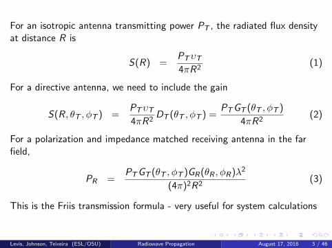
For an isotropic antenna transmitting power PT , the radiated flux densityat distance R is

S(R) =PTυT

4πR2(1)

For a directive antenna, we need to include the gain

S(R, θT , φT ) =PTυT

4πR2DT (θT , φT ) =

PT GT (θT , φT )

4πR2(2)

For a polarization and impedance matched receiving antenna in the farfield,

PR =PT GT (θT , φT )GR(θR , φR)λ2

(4π)2R2(3)

This is the Friis transmission formula - very useful for system calculations


Excepting for the ohmic losses in the antennas, included in υT and υR , weneglected all other losses in the previous equation. We can include them by

PR =PT GT (θT , φT )GR(θR , φR)λ2

(4π)2R2TgasTrainTimpTpolTcoupling

where

Tgas = exp

(−∫

pathαgas dl

)(4)

Train = exp

(−∫

pathαrain dl

)(5)

These are due to the fact that flux density will be proportional to e−αx ina scattering medium, but α may change along the path


It is often easier to work with this equation in dB as

PR,dbW = PT ,dbW − Lsys,db (6)

where the system loss Lsys,db is given by

Lsys,db = 20 log10 Rkm + 20 log10 fMHz + 32.44 + Lgas,db + Lrain,db + Lpol ,db

+Limp,db + Lcoup,db − GTdb − GRdb (7)

and

Ldb = −10 log10 T (8)


This gives

Lgas,db =

∫path

αgas,db dl (9)

and

Lrain,db =

∫path

αrain,db dl (10)

where αgas,db and αrain,db are the “specific attenuation” due to gas andrain in dB/km

αgas,db = 4.34 αgas

αrain,db = 4.34 αrain (11)

Thus to get the total loss along a path, we need to integrate the specificattenuations over the path


Practical considerations:

Consider a 1 MWatt transmitter (PT = 106 Watts)

Consider a sensitive receiver with 100 ohm input impedance that candetect 1 µvolt

PR,min = V 2/R =(10−6

)2/100 = 10−14

Maximum tolerable system loss: 10−14/106 = 10−20 or 200 dB

Thus, system losses greater than 200 dB are not very practical formost systems


Another sample problem: Communicating with Galileo

Approximate distance to Galileo: = 628× 106 km

Let’s use a 2 GHz system: fMHz = 2, 000

Neglecting system and atmospheric losses we get

Lsys,db = 20 log10 Rkm + 20 log10 fMHz + 32.44− GTdb − GRdb

= 175 + 66 + 32.44− GTdb − GRdb

= 273.44− GTdb − GRdb (12)

Assume Galileo has a 10 dBi gain (high gain antenna never opened)and transmits 20 W, then

PR = 13− 273.44 + 10 + GRdb (13)

It’s pretty clear we need a high gain antenna on the ground and a goodreceiver with low F - JPL quotes 10−20 watts as being received!


III. Atmospheric gas attenuation

Gas molecules in the atmosphere are able to absorb microwave power- it is re-emitted as thermal noise

Effects not very significant below 10 GHz

Most significant around molecular resonance frequencies, in particularoxygen and water vapor; ITU-R Recommendation P. 676-7.

Resonance frequencies: water - 22.3, 183.3, 325.4 GHz, oxygen - 60,118.7 GHz

Density of resonances increases greatly at higher frequencies

Specific attenuation depends on atmospheric composition whichvaries with altitude

Pressure broadening changes line shapes at different altitudes

Tool available atwww.rcru.rl.ac.uk/show.php?page=njt/ITU/ITU676-6


10 100 10000.001

0.01

0.1

1

10

100

1000

Frequency (GHz)

Spe

c. a

tten

(dB

/km

)

OxygenWater VaporBoth


10 100 10000.001

0.01

0.1

1

10

100

1000

Frequency (GHz)

Spe

c. a

tten

(dB

/km

)

0 km10 km

50 55 60 65 700.001

0.01

0.1

1

10

Frequency (GHz)

Spe

c. a

tten

(dB

/km

)

0 km10 km20 km


IV. Total attenuation on a path

Horizontal paths are easy since atmospheric gases are usually uniformhorizontally

Lgas,db =

∫αgas,db dl = αgas,dbL (14)

Vertical or slant paths require integration over path

Typical models for atmospheric variations are like

ρ = ρ0 exp (−h/hs,w ) (15)

or we can use measurements of atmospheric composition

Results are often presented as an “equivalent” L by which αgas,db atthe ground can be multiplied to get through the total atmosphere

We will just rely on the figure for total vertical attenuation throughthe atmosphere

Higher frequencies have many resonances


1 10 100 10000.001

0.01

0.1

1

10

100

1000

Frequency (GHz)

Zen

ith a

tten

(dB

)

0 km5 km10 km


Attenuation on slant paths can be obtained from the correspondingvertical path through

Lgas,slant(h1, h2) =

∫ s2

s1

αgas,db(s) ds =

∫ h2

h1

αgas,db(h) csc θ dh

= Lgas,vert csc θ (16)

For attenuations at two different angles,

Lg (θ1)

Lg (θ2)=

csc θ1csc θ2

=sin θ2sin θ1

(17)

Note these relations do not apply for θ < 10 degrees due to Earthcurvature and refraction


dh dS

θ

Ground Distance

Altitude h


Direct Transmission, Part Two

1 Rain attenuation

2 Specific attenuation for rain

3 Rain statistical information

4 Probability of outage predictions


I. Rain attenuation

Rain also can cause attenuation along atmospheric paths, usuallynegligible for f < 5 GHz

Can cause serious outages as frequency increases

A statistical approach is necessary for discussing rain fades - averagenumber of hours per year to obtain given attenuation

Statistics will vary from location to location!

We will therefore need two types of information: one for attenuationon a path given rain rate (deterministic) and one for probability ofrain rate (statistical)

Systems can be designed with a “rain margin” to allow continuedfunction even during rain events


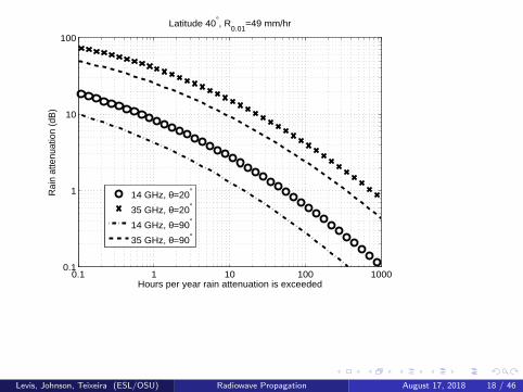
0.1 1 10 100 10000.1

1

10

100

Hours per year rain attenuation is exceeded

Rai

n at

tenu

atio

n (d

B)

Latitude 40°, R0.01

=49 mm/hr

14 GHz, θ=20°

35 GHz, θ=20°

14 GHz, θ=90°

35 GHz, θ=90°


II. Specific attenuation for rain

As with atmospheric gases, we can talk about a specific attenuationfor rain, αrain,db in dB/km

Specific attenuation must be integrated over path to get totalattenuation - this is more difficult for rain

We can use theory to derive a specific attenuation for rain through

Drop size distribution n(r)- number density per drop diameterMie scattering theory for a sphere to obtain amount of power absorbedand scattered out of incident beam for one sphere - “extinction crosssection”Integration over size distribution to get total power lossThis is power lost in a differential volume, leads to a differentialequation that shows flux density ∝ e−αx


It turns out that both theory and experiment lead to a simpler formfor rain specific attenuation as

αrain,db = krRarr (18)

kr and ar are tabluated coefficients and Rr is the rain rate in mm/hr

We will use the plots in the book that give kr and ar for bothhorizontal and vertical polarizations

These coefficients are functions of frequency since drop scattering andaborption efficiency changes with frequency


1 10 100 1000

10−4

10−3

10−2

10−1

100

Frequency (GHz)

k r coe

ffici

ent

HV


1 10 100 10000.6

0.8

1

1.2

1.4

1.6

Frequency (GHz)

a r coe

ffici

ent

HV


1 10 100 10000.01

0.1

1

10

100

Frequency (GHz)

Rai

n S

peci

fic A

ttenu

atio

n (d

B/k

m)

H pol, 10 mm/hrH pol, 50 mm/hrH pol, 100 mm/hrV pol


III. Rain statistical information

We now have an equation relating rain specific attenuation to rainrate Rr

If we have statistical information on Rr for a given location, we canthen obtain statistical information on α through α = krR

arr

Several sources available for this information:

Local measurements: always best but usually not availableNational Weather Service or National Oceanic and AtmosphericAdministration in USOther global models

Note that “tails” of the distribution are most important because it isthe heaviest rains that give the most serious attenuation

The ITU-R model we will use for predicting rain attenuation focusesinstead of the rain rate exceeded 0.01 percent of the time, Rr ,0.01


20

25

30

35 40

45

50

55 60

65

70

75

80

25

30

35

50

40

5515 60

85

45

85

6565

15

15

15

50

7570

35

90

20

70

25

25

20

40

25

120oW 108oW 96oW 84oW 72oW

25oN

30oN

35oN

40oN

45oN

50oN


IV. Probability of outage predictions

So far we have models for rain specific attenuation and some info onprobability of rain rates

We still don’t have total attenuations though because we haven’tintegrated over paths

Difficult to do this precisely because rain properties vary horizontallyand vertically!

Lots of models available; ITU-R studies provide recommendations onuse


All of the total path attenuation models are based on either

Lrain,db =

∫path

αrain,db(l) dl ≈ αrain,db(0)Leff (19)

where αrain,db(0) is the specific attenuation at sea level and Leff is an“effective” path length, or

Lrain,db =

∫path

αrain,db(l) dl ≈ aRbeff L (20)

where Reff is an “effective” rain rate. Empirical methods are usually usedto find these quantities.


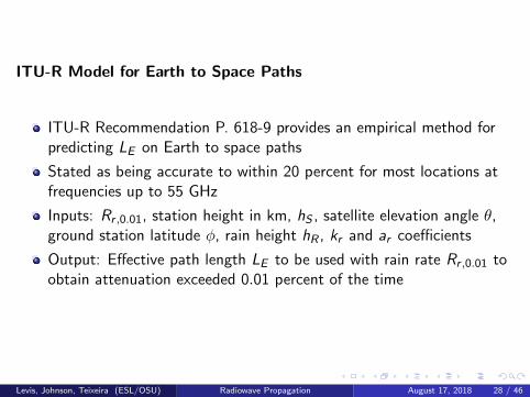
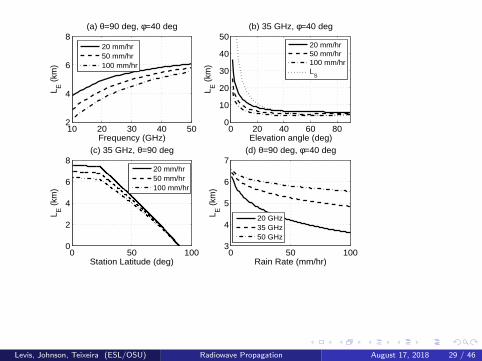
ITU-R Model for Earth to Space Paths

ITU-R Recommendation P. 618-9 provides an empirical method forpredicting LE on Earth to space paths

Stated as being accurate to within 20 percent for most locations atfrequencies up to 55 GHz

Inputs: Rr ,0.01, station height in km, hS , satellite elevation angle θ,ground station latitude φ, rain height hR , kr and ar coefficients

Output: Effective path length LE to be used with rain rate Rr ,0.01 toobtain attenuation exceeded 0.01 percent of the time


10 20 30 40 502

4

6

8

Frequency (GHz)

L E (

km)

(a) θ=90 deg, φ=40 deg

20 mm/hr50 mm/hr100 mm/hr

0 20 40 60 800

10

20

30

40

50

Elevation angle (deg)

L E (

km)

(b) 35 GHz, φ=40 deg

20 mm/hr50 mm/hr100 mm/hrL

S

0 50 1000

2

4

6

8

Station Latitude (deg)

L E (

km)

(c) 35 GHz, θ=90 deg

20 mm/hr50 mm/hr100 mm/hr

0 50 1003

4

5

6

7

Rain Rate (mm/hr)

L E (

km)

(d) θ=90 deg, φ=40 deg

20 GHz35 GHz50 GHz


ITU-R Model for Earth to Earth Paths

ITU-R Recommendation P. 530-12 provides an empirical method forpredicting LE on Earth to Earth paths

LE =d

1 + d/d0

where d is the path distance in km and

d0 = 35e−0.015Rr,0.01 Rr ,0.01 ≤ 100

d0 = 7.81 Rr ,0.01 > 100 (21)

with Rr ,0.01 in mm/hr.The quantity d0 is an average horizontal extent of the rain, and decreasesfrom 35 km at low rain rates to 7.81 km at very high rain rates.


Probability Scaling

The Preceeding models determine the attenuation exceeded 0.01 percentof the time:

Lrain,0.01 =(krR

arr ,0.01

)LE

A “probability scaling” approach is recommended to obtain attenuationsexceeded p percent of the time. For Earth-to-space paths

Lrain,p = Lrain,0.01

( p

0.01

)−[0.655+0.033 ln(p)−0.045 ln(Lrain,0.01)−β(1−p) sin θ]

where

β = 0 p ≥ 1 or |φ| ≥ 36◦

β = −0.005 (|φ| − 36◦) p < 1 and |φ| < 36◦ and θ ≥ 25◦

β = −0.005 (|φ| − 36◦) + 1.8− 4.25 sin θ otherwise

This approach is specified as accurate for p ranging from 0.001 to 5percent (see equations in book for Earth-to-Earth paths).


Use of rain attenuation models enables us to ascertain how manyhours of fades of a given number of dB to expect per year

Systems can be designed to have enough S/N ratio to function evenduring these fades

This is not always possible with practical satellite systems however

Problem increases with frequency, so satcom and radar systemsoperating at f > 10 GHz can expect significant outage times due torain

Program for the ITU-R model available via course website

Frequency scaling approaches also available to scale attenuationsobserved at one frequency into another at the same location


Direct Transmission, Part Three

1 Rain attenuation example

2 Site diversity improvements

3 Scintillations on atmospheric paths

4 Look angles to geostationary satellites


I. Rain attenuation example

12 GHz Earth to satellite link with the ground station location nearColumbus, Ohio (latitude ≈ 40◦, station height 0 km). The satellite isobserved at range 38,000 km from the ground station at elevation angle40 degrees. Suppose the satellite transmitter transmits 120 Watts ofpower in a 24 MHz bandwidth using circular polarization, and has anantenna gain of 46 dBi. Suppose also that the receiver has a noise figureof 6 dB and the receive antenna gain is 30 dBi.

Given that the signal to noise ratio required for the system to function is10 dB, how many hours per year (on average) will the system fail?


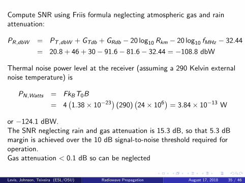
Compute SNR using Friis formula neglecting atmospheric gas and rainattenuation:

PR,dbW = PT ,dbW + GTdb + GRdb − 20 log10 Rkm − 20 log10 fMHz − 32.44

= 20.8 + 46 + 30− 91.6− 81.6− 32.44 = −108.8 dbW

Thermal noise power level at the receiver (assuming a 290 Kelvin externalnoise temperature) is

PN,Watts = FkBT0B

= 4(1.38× 10−23

)(290)

(24× 106

)= 3.84× 10−13 W

or −124.1 dBW.The SNR neglecting rain and gas attenuation is 15.3 dB, so that 5.3 dBmargin is achieved over the 10 dB signal-to-noise threshold required foroperation.Gas attenuation < 0.1 dB so can be neglected


From rain rate map, Rr ,0.01 in Columbus around 45 mm/hr.kr around (0.024,0.024), ar around (1.12,1.18) for h and v polarizationsfrom figuresCombine using equation for circular pol to get kr = 0.024, ar = 1.15.ITU-R Earth-to-space model gives LE = 3.93 km so

Lrain,0.01 = 3.93×(0.024× 451.15

)= 7.5 dB (22)

Use probability scaling to get other percentages; note scaling is hard toinvert so may need an iterative or graphical method to find whatpercentage gives 5.3 dB attenuationGraph on the next page shows 0.025 percent, or around 2.2 hours per year


0.001 0.01 0.1 10.5

1

2

5

10

20

Percent of time rain attenuation is exceeded

Rai

n at

tenu

atio

n (d

B)

12 GHz, Latitude 40°, R0.01

=45 mm/hr


II. Site diversity improvements

Serious rain attenuation usually only happens over a small horizontalextent - heavy rain cells are finite

Thus if we have two antennas separated by a wide distance it isunlikely that both would have serious rain fades at the same time

This is a “diversity” concept - use multiple antennas to avoid fades

Signals from antennas can be combined either by switching toantenna with highest power or always using both in a varying ratio


Two quantities defined: diversity gain and diversity improvement

Dependence on distance: measurements done at OSU showsaturating exponential curve

An empirical model was developed from this data

Models are necessary because buying and placing another antennamay not be easy!


0.001 0.01 0.110

100

Percent of time rain attenuation is exceeded

Rai

n at

tenu

atio

n (d

B)

One antennaTwo antennas

I

Gd


0 5 10 15 20 25 30 350

1

2

3

4

5

6

Distance between antennas (km)

Div

ersi

ty G

ain

(dB

)

14 GHz, θ=20°

2 dB6 dB10 dB


III. Scintillations on atmospheric paths

As we know, the atmosphere is not a homogeneous medium, andsmall variations cause variations in propagated signals

All radio paths will observe some small fluctuations

These should not be confused with system effects!

Scintillations are usually larger at lower elevation angles because thereis more path length in which the atmosphere can vary

May appear to be amplitude or angle of arrival variations dependingon scan rate

Twinkling of stars is a scintillation phenomenon! Important problemfor optical astronomy


IV. Look angles to geostationary satellites

Satellites orbiting at 35, 900 km have an orbital period equal to therotation of the Earth - thus they stay fixed in the sky

This makes ground station design simple - no tracking required

Note this is pretty far away however; it remains to be seen how thesesystems will compare with LEO satellite for PCS systems now underdevelopment

It is fairly straight forward to derive the angles (∆,Az) at which aground antenna should be oriented given the station latitude θ′,longitude φ′, and sub-satellite longitude φ0


Station in Northern hemisphere: azimuth is Az = π + β for a satellite westof the station, Az = π − β for a satellite east of the station.

cos δ = cos θ′ cos(φ′ − φ0

)(23)

cosβ = tan θ′ cot δ (24)

To find the elevation angle use the law of cosines

R2 = R2ε + (Rε + RS )2 − 2Rε (Rε + RS ) cos δ (25)

and

CB = R sin ∆ (26)

= CO − OB = (Rε + RS ) cos δ − Rε (27)

so that

sin ∆ =(Rε + RS ) cos δ − Rε

R(28)


- 0

E

A

’

’θ


C

O

S

R

B

RE A

RE

RS


Documents

Review noise concepts Direct transmission - Friis formula