Embed Size (px)
Citation preview

U. S. Department yaso
AD-A26 407 of TransportationUnited States
]II1111 ~~ H Coast Guard
Report of theInternational Ice Patrolin theNorth Atlantic
HC- 130 AIRCRAFT25 years of Ice Patrol Service
93-01032 D I11,11111 EL ECTF
1988 Season SJA21i93§Bulletin No. 74 ...CG- 188-43 FAPPcVGzeIli
93 1 21008

521" N
No!'e Dan~e Bay
48 0 N Newfoundland
460 N xAva~on Ctr.annel
\ -~---Grand Banks
440 N ~ ~Newfoundland
420 N
400 N580 W 54" W 50, W 46' W
Figure 1. Bathymetry of the Grand Banks of Newfoundland.

U&SDepjnrtmnef.t "MLING ADDRES&
um~tw stat., ods 2 100 2 nd S t. S:-W:-U~Skfi S Washington, D.C. 20593CoastGuaM (202)267-1 450
JL 23 3)Bulletin No. 74
REPORT OF THE INTERNATIONAL ICE PATROLIN THE NORTH ATLANTIC
SEASON OF 1988
CG-1 88-43
FOREWORD
Forwarded herewith is bulletin No. 74 of the International IcePatrol, describing the Patrol's services, ice observations and
conditions during the 1988 season.
J. \,V I. ',N4• OODU.ia• C.]S L'a~t Guaur4
A~,'• C hicf, OQ"kc A Na•ig250
S!c-,y and Wacrway riScls
DISTRIBUTION--SDL No.
a b c d je f g h i kino0pPqi r s t u vlw !yjzi
4
D 60
NON-TANDARD DISTRIBUTION: B:a G-NIO only, B:b LANTAREA (5), PACAREA (1), B:c First,
Fifth Districts only, C:a CGAS Cape Cod, Elizabeth City only, C:q LANTAREA only,S14L CG-4
INTERNATIONALICE PATROL1988 ANNUAL REPORT
CONTENT,
5 INTRODUCTION7 SUMMARY OF OPERATIONS11 ICEBERG RECONNAISSANCE AND COMMUNICATIONS13 ENVIRONMENTAL CONDITIONS, 1988 SEASON25 ICE CONDITIONS, 1988 SEASON49 DISCUSSION OF ICE AND ENVIRONMENTAL CONDITIONS50 REFERENCES51 ACKNOWLEDGEMENTS
APPENDICES
53 A. List of Participating Vessels, 198861 B. 1988 International Ice Patrol Drifting Buoy Program81 C. Upgrade of Environmental Inputs to Iceberg Forecasting Models87 D. Use of Air-Deployed Bathythermogaphs (AXBTs) durinr the 1988 HiP
Season101 E. liP's Side-Looking Airborne Radar (SLAR) Experiment 1988
Accesion For
M IS CRA&IDTIC TABUr . ino fcid uc
DTIC Q"UA L77Y QL$ -T.C' ------------- t-----o
Avaiiabiity Codes
Aval and I orDist Special
-- --- ---

Introduction
This is the 74" annual report of the IntierabonaI Ice Patrol
Service in the North Atlantic This report contains information on IcePatrol operations, environmental conditions, and ice conditons for 1988The U S. Coast Guard conducts the International Ice Patrol Ser,,-ce inthe North Atlantic under the provisions of U S Code, Title 46, Sections738, 738a through 738d, and the International Convention tor the Safetyof Life at Sea (SOLAS), 1974, regulations 5ý8. This servwce was initi-ated shortly aflter the sinking of the RMS TITANIC on April 15 1912
Commander. international Ice Patrol. working under Com-mander, Coast Guard Atlantic Area. directs the Intemationai Ice Patrolfrom offices located at Groton, Connecticut The International Ice Patrolanalyzes ice and environmental data, prepares the daily ice bulie'insand facsimile charts. and replies to any requests for special ice informa-tion. It also controls the aerial Ice Reconnaissance Detachment andany surface patrol cutters when assigned. both of which patrol thesoutheastern, southern, and southwestern limits of the Grand Banks ofNewfoundland for icebergs. The International Ice Patrol makes twice-daily radio broadcasts to warn manners of the limits of iceberg diStnbu-lion.
Vice Admiral D. C. Thompson was Commander, Atlantic Area.until June 29, 1988, and Rear Admiral J. C, Irwin was Commander.Atlar~tic Area, from June 29, 1988. to the end of the 1988 ice year. CDRS. R_ Osmer was Commander, International Ice Patrol, during the entire1988 ice year.
5

Summary ofOperations, 1988
From April 13 to August 2, Gander, Newfoundland, one week lIP's computer model
1988, the International Ice Patrol out of every two. The season consists of a routine which pre-
(liP), a unit of the U.S. Coast officially closed on Augusl 2. 1988 dicts the drifl of each iceberg, and
Guard, conducted the International a routine whch predicts the
Ice Patrol Service, which has been Watchstanders at lIP's deterioration ot each iceberg The
provided annually since the Operations Center in Groton, drift prediction program uses aConnecticut, analyze the iceberg historical current file to drift thesinking of the RMS TITANIC on
April 15, 1912. During past years, sighting information from the icebergs. This histoncal data file
Coast Guard ships and/or aircraft ICERECDET. along with sighting is mrodified weekly using satellite-
have been patrolling the shipping information from commercial *racked ocean drifting buoy data to
lanes off Newfoundland within the shipping and Atmospheric Envi- take into account local, short-termarea delineated by 40"N -52"N, ronment Service (AES) of Canada current fluctuations Murphy and39W 57W (Figure 1, inside front sea iceficeberg reconnaissance Anderson (1985) descbe the lIPcover), detecting icebergs, and flights. The lIP Operations Center drift model in more detail, alongwarning mariners of these haz- received 35,129 iceberg sightings with an evaluation of the model.
ards. During 1988, Coast Guard from these sources in 1988,HC-130 aircraft flew 40 ice recon- compared to 7,031 in 1987. Only The lIP iceberg deteriora-
those iceberg sightings within lIP's tion program uses daily wind, seanaissance sorties, logging over257 flight hours. The AN/APS-135 operations area (40°N - 521N, surface temperature, and wave
Side-Looking Airborne Radar 39 0W - 57 0W) are entered into the height information from the U S(SLAR), which was introduced lIP iceberg drift prediction corn- Navy Fleet Numerical Oceanogra-
into Ice Patrol duty during the puter model (ICEPLOT). The phy Center (FNOC) to melt the1983 season, again proved to be watchstanders determine whether icebergs. Appendix C discusses
an excellent all-weather tool for the sighting is a resight of an recent improvements FNOC hasthe detection of both icebergs and iceberg lIP already has on made to these products. Ander-sea ice. In addition, the AN/APS- ICEPLOT, or whether the sighting son (1983) and Hanson (1987)
131 SLAR on the Coast Guard is of a new iceberg which had not describe the UlP deteriorationHU-25B aircraft was evaluated, been previously reported. Iceberg model in detail. It is the combinedand the HU-25B was used opera- sightings near the Newfoundland ability of the SLAR to detect
tionally for the first time on one ice coast are not entered into the icebergs in all weather, and thereconnaissance sortie. computer model due to lack of lIP's computer models to estimate
ocean current information in the iceberg drift and deterioration,Aircraft deployments were model in these areas to drift the which has enabled lIP to reduce
made on February 17 to 21, icebergs. Each sighting is labelled its ICERECDET operations fromMarch 3 to 16, and March 28 to in the computer as either a resight weekly deployments to every other
April 1 to determine the pre- or a new sighting. During the week deployments.season iceberg distribution. 1988 ice year, an estimated 1340
Based on the last pre-season icebergs were sighted in lIP'sdeployment, the 1988 International operations area (south of S2°N),Ice Patrol season opened on April compared to 755 in 1987. 11600113. From this date until August 3, these were entered into liPs1988, an aerial Iceberg Recon- computer model, compared to 686
in 1987.naissance Detachment(ICERECDET) operated from
7

Table 1. Source of International Ice Patrol Iceberg Reports by Size.
PercentSighting Source Growler Smail Medium Large Radar TargeW Total ot TotalCoast Guard (liP) 43 315 289 168 39 854 39,0Canadian AES 17 210 268 115 28 638 29.2Commercial Ship 37 76 266 78 44 501 22.9Offshore Oil Industry 6 42 51 31 1 131 60Lighthouse/Shore 0 1 10 6 0 17 0.8DOD Sources 0 1 8 6 0 15 0.7Other 0 3 11 3 13 30 1.4Total 103 648 903 407 125 2186 100.0
Table 1 shows the total During the 1988 ice year, than 900 icebergs crossing 48CNiceberg sightings reported to liP in an estimated 187 icebergs drifted as extreme. With 187 icebergs1988 (including resights) which south of 48ON latitude, compared drifting south of 48,N, 1988 waswere in liP's operations area and to 318 icebergs drifting south of deemed a fight year.away from the Newfoundland 48°N during 1987. The averagecoast, broken down by the sighting number of icebergs drifting south On April 15, 1988, l1Psource and iceberg size. lIP of 48°N from 1900 to 1987 is 403 paused to remember the 761ICERECDET, AES, and commer- (Alfultis, 1987). With 187 icebergs anniversary of the sinking of thecial shipping continue to be the drifting south of 48°N, 1988 was RMS TITANIC. During an icethree major sources of iceberg less than the average. The reconnaissance patrol, twosighting reports. Appendix A lists number of icebergs crossing 48°N memorial wreaths were placedall iceberg sightings received from during 1988 was less than the near the site of the sinking tocommercial shipping, regardless SLAR reconnaissance era aver- commemorate the nearly 1500of the sighting location, age. It is important to note, lives lost.
however, that this SLAR eraTable 2 fists monthly average is based on only five Six satellite-tracked ocean
estimates of the total number of years of data. drifting buoys were deployed toicebergs that crossed 48°N for the provide operational data for liP'spre-Intemational Ice Patrol era, liP defines those ice years iceberg drift model These buoysand for the ship, aircraft visual, with less than 300 icebergs were the same standard-sizeand aircraft SLAR reconnaissance crossing 48°N as light or low ice drifting buoys liP has beeneras. Table 3 compares the years; those ice years with 300 to deploying for thirteen years Fourestimated number of icebergs 600 icebergs crossing 48°N as of these buoys were later recov-crossing 48°N for each month of average or intermediate; those ice ered by USCGC NORTHWIND for1988 with the monthly mea, years with 600 to 900 icebergs re-use. The drift data from thesenumber of icebergs crossing 48°N crossing 48°N as heavy or severe; buoys are discussed in Appendixfor each of the four different eras. and those ice years with more B.8

In addition, four mini- Table 2. Total Icebergs South of 46- N - The four periods shown aredrifting buoys were deployed in pre-International Ice Patrol (1900- 12), ship reconnaissance (1913-45),liP's operations area as part of a aircraft visualreconnaissance (1946-82), and SLAR reconnaissancejoint IIP-Naval Oceanographic (1983-87).Research and DevelopmentActivity evaluation. One AES Total To1al Tota1 Tota1 1988mini-drifting buoy was also 1900-12 1913-45 1946-82 1983-87deployed by lIP together with one OCT 27 80 2 3 0lIP standard-size drifting buoy. NOV 13 93 4 11 0These mini-drifting buoys are DEC 38 42 11 14 0
smaller with a lower cost per unit JAN 33 87 65 13 0FEB 79 372 273 239 0than the standard-size buoy. lIP is MAR 89& 1204 1172 442 8
evaluating these mini-drifters for APR 1537 3308 3131 1636 95possible future operational use. MAY 1611 5472 2993 1242 33The results of this evaluation are JUN 1004 2514 1865 793 20presented in Appendix B. JUL 423 773 489 567 19
AUG 160 229 100 138 10Prior to the start of the SEP 58 188 10 41 2
1988 lIP season, lIP evaluated anAir-Deployed eXpendable Total 5,881 14.362 10,115 5,139 187
BathyThermograph (AXBT)system. The AXBT measurestemperature with depth, andtransmits the data back to theaircraft. Based on the results ofthe evaluation, lIP put together an Table 3. Average Number of Icebergs South of 46' N - The four periodsAXBT system and operationally shown are pre-tnternational Ice Patrol (1900-12), ship reconnaissancedeployed twelve AXBTs during the 4'1913-45), aircraft visual reconnaissance (1946-82), and SLAR recon-1988 liP season. The results of naissance (1983-87).the evaluation and operational useof the AXBT system are presented Avg Avg Avg Avg 1988in Appendix D. 1900-12 1913-45 1946-82 1983-87
OCT 2 2 0 1 0The temperature data NOV 1 3 0 2 0
from the AXBTs were sent to the DEC 3 1 0 3 0Canadian Meteorological and JAN 2 3 2 3 0Oceanographic Center (METOC) FEB 6 11 7 48 0
in Halifax, Nova Scotia, Canada, MAR 69 36 32 88 8
the U.S. Naval Eastern Oceanog- APR 118 100 85 327 95raphy Center (N EOC) in Norfolk, MAY 124 166 81 248 33
JUN 77 76 50 159 20Virginia, and FNOC. They use the JUL 32 23 13 113 19AXBT data as inputs to their AUG 12 7 3 28 10ocean temperature models. IlP SEP 4 6 0 8 2directly benefits from its AXBTdeployments by having improved Era 452 435 273 1,028 187
ocean temperature data p•,ivided Average
9

to its iceberg deterioration model.To further enhance the quality ofenvironmental data used in itsiceberg models, lIP also providedweekly drifting buoy drift and seasurface temperature (SST)histories, and SLAR ocean featureanalyses to METOC and NEOC.They used this information in theirwater mass and SST analyses.
No U. S. Coast Guardcutters were deployed to act assurface patrol vessels this yearUSCGC NORTHWIND wasdeployed from June 3 to 27 to actas a surface truth vessel for aninternational SLAR evaluationexperiment, SLAREX '88. TwoU.S. Coast Guard and two Cana-dian AES SLAR-equipped aircraftparticipated in SLAREX '88. Theprimary goal of the experimentwas to evaluate the ability of theAN/APS-131 SLAR on the HU-25B aircraft to detect icebergs,The results of SLAREX '88 arepresented in Appendix E.
The 1988 season markedthe 25th full year of lIP service forthe HC-130 'Hercules' aircraft. A'Hercules' flew one ice reconnais-sance patrol in 1963. The HC-1 30assumed the Ice Patrol aerialreconnaissance responsibilities forthe 1964 season until the present.
10

Iceberg Reconnaissanceand Communications
During the 1988 Ice Patrol Newfoundland. During the active Aerial ice reconnaissanceyear (from October 1, 1987, season, ice observation flights was conducted with SLAR-through September 30, 1988), 86 located the southwestern, south- equipped HC-130H aircraft, and,aircraft sorties were flown in ern, and southeastern limits of for the first time, with a SLAR-support of the International Ice icebergs. Logistics flights were equipped HU-258 aircraft. ThePatrol. These included pre- necessary to support the patrol US. Coast Guard HC-130Hseason flights, ice observation aircraft due to aircraft mainte- aircraft deployed from Coast Airflights during the season, post nance problems. Post season Station Elizabeth City, Northseason flights, logistics flights, and flights were made to check on the Carolina. The U.S. Coast GuardSLAR research flights. Pre- iceberg distribution, to retrieve HU-25B aircraft deployed fromseason flights determined iceberg parts and equipment from Gander, Coast Guard Air Station Capeconcentrations north of 48oN. and to close out all business trans- Cod, Massachusetts, The HC-These iceberg concentrations actions from the season. The 130H and HU-25B aircraft bothwere needed to estimate the time SLAR research flights were in participated in SLAREX "88. HG-when icebergs would threaten the support of SLAREX '88. 130 aircraft were used on logisticsNorth Atlantic shipping lanes in the flights. Table 4 shows aircraft usevicinity of the Grand Banks of during the 1988 ice year.
Aircraft Sorties Flight HoursDeployment
Pre-season 16 92.7Regular Season 50 272.0Post Season 3 16.9SLAR Research 17 53.2
Total 86 434.8
Iceberg Reconnaissance Sorties by Month
Month Sorties Flight Hours
Feb 3 21.0Mar 4 28.1
Apr 7 43.7May 8 51.3Jun 11 68.8Jul 5 32.1Aug 2 12.4
Table 4. Aircraft use during theTotal 40 257.4
1985 liP Year (October 1, 1987 -September 30, 1988)
11

Table 5. Iceberg and Sea Surface Temperature Reports.
Number of ships furnishing Sea Surface Temperature (SST) reports 39Number of SST reports received 200Number of ships furnishing ice reports 255Number of ice reports received 711First Ice Bulletin 130000Z APR 88Last Ice Bulletin 021200Z AUG 88Number of facsimile charts transmitted 110
The lIP prepares the ice Canadian Forces METOC, For the first timp, lIP wasbulletin warning mariners of the Halifax/CFH, as well as AM Radio directly linked in 1988 to Canadiansouthwestern, southern, and Station Bracknell/GFE, United Coast Guard Radio St John's/southeastern limits of icebergs Kingdom, are radiofacsimile VON, Ice Operations St. John's,twice a day for broadcast at OOOOZ broadcasting stations which used Ice Centre Ottawa, and theand 1200Z. The lIP also prepares Ice Patrol limits in their broad- offshore oil industry via an elec-a facsimile chart graphically casts. Canadian Coast Guard tronic mail system with telex as adepicting these limits for broadcast Radio Station St. John's/ VON and backup. Canadian Radio Stationat 1600Z. U.S. Coast Guard U.S. Coast Guard Communica- St John'sNON passed all icebergCommunications Station Boston, tions Station Boston/NIK provided sighting reports it received to IlIPMassachusetts, NMF/NIK, was the special broadcasts. via Ice Operations St. John's. Iceprimary radio station used for the Operations St John's converteddissemination of the daily ice The International Ice the iceberg sighting report to thebulletins and facsimile charts. Patrol requested that all ships computer compatible joint AES/IIPOther transmitting stations for the transiting the area of the Grand iceberg code. This ensured betterOOOOZ and 1200Z ice bulletins Banks report ice sightings, accountability and more timelywere Canadian Coast Guard weather, and sea surface tem- receipt of the iceberg sightingRadio Station St. John's/VON, Ca- peratures via the above communi- reports. I'- and AES reconnais-nadian Forces Meteorological and cations/radio stations. Response sance detachments have beenOceanographic Center (METOC) to this request is shown in Table 5. using the computerized code sinceHalifax, Nova Scotia/CFH, and Appendix A lists all rontributors. the 1986 season. The offshore oilU.S. Navy LCMP Broadcast Commander, International Ice industry conducts aerial iceStations Norfolk/NAM; Thurso, Patrol extends a sincere thank you reconnaissance in the vicinity of oilScotland; and Keflavik, Iceland. to all stations and ships which exploration on the Grand Banks.
contributed. Their sighting reports are transmit-ted directly to Groton.
12
Environmental Conditions1988 Season
The wind direction along the The following discussion summa- displaced the Icelandic Low to theLabrador and Newfoundland rizes the anvironmental conditions west, and caused a -4 rrb anom-coasts can affect the iceberg along the Labrador and New- aly in the Labrador Sea (Marinersseverity of each ice year. The foundland coasts for the 1988 ice Weather Log, 1988b). The windsmean wind flow can influence year. in March were near normal,iceberg drift. Dependent upon however, with northwesterly winds'vvnd intensity and duration, January: The monthly mean along the Labrador Coast andicabergs can be accelerated along pressure of the Icelandic I ow was westerly winds east of Newfound-or driven out of the main flow of 10 mb lower in January than land (AES, 1988).the Labrador Current. Departure normal (Figure 2). This resulted infrom the Labrador Current nor- stronger, slightly more westerly April: In April, the Azores-mally slows their southerly drift, winds along the Labrador Coast Bermuda High usually begins toand in many cases speeds up (AES, 1988), and strong westerly build in strength while the Ice-their rate of deterioration, winds over the waters east of landic Low begins to decrease in
Newfoundland in January. intensity (Mariners Weather Log,The wind direction and air tern- 1988c). In 1988, the Azores-perature affect the iceberg severity February: A double-centered Bermuda High was near its normalof each ice year in an indirect way Icelandic Low formed this month position and intensity (Figure 5).by influencing the extent of sea on either side of Iceiand (Figure However, with a monthly meanice. Sea ice protects the icebergs 3). This is not unusual, but when pressure 4 mb lower than normal,from wave action, the major agent a double-centered Icelandic Low the Icelandic Low was moreof iceberg deterioration. If the air forms, the two centers are usually intense and farther west thantemperature and wind direction near Denmark Strait and off normal. This resulted in strong,are favorable for the sea ice to Norway (Mariners Weather Log, northeasterly winds along Labra-extend to the south and over the 1988b). The two lows were also dor and eastern NewfoundlandGrand Banks of Newfoundland, deeper ihan normal. This led to a rather than the normal fighter,the icebergs will be protected -8 mb anomaly centered in Davis more northerly winds.longer as they drift south. When Strait (Mariners Weather Log,the sea ice retreats in the spring, 1988b), and a stronger than May: In May, the Azores-Ber-large numbers of icebergs are left normal northwesterly flow along muda High began to dominate thebehind on the Grand Banks. Also, the Labrador Coast. A westerly North Atlantic (Figure 6). It wasif the time of sea ice retreat is flow dominated the waters east of slightly stronger than normal, butdelayed by below normal air Newfoundland. The flow was storm activity to the north kept ittemperatures, the icebergs will be more offshore than normal in both from its normal expansion (Mari-protected longer, and a longer of these areas (AES, 1988). ners Weather Log, 1988c). Thethan normal ice season can be resulting flow pattern alongexpected. The opposite is true if March: The Azores-Bermuda High Labrador and eastern Newfound-the southerly sea ice extent is less dominated the western North land was light northeasterly windsthan average, or if above normal Atlantic in March, and its monthly rather than the normal lightair temperatures cause an early mean pressure was 6 mb higher southwesterlies.retreat of sea ice from the Grand than normal (Figure 4). ThisBanks.
13

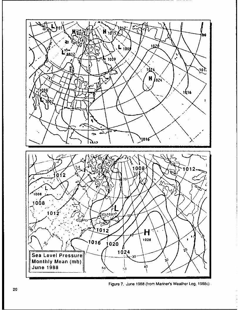
June: With a monthly mean Septemtbr: Both the Azorespressure 4 nib higher than normal, Bermuda High and icetarKnkc Lowthe Azores-Bermuda High was were stronger than normal inagain stronger than normal in September (Figure 101 TheJune (Figure 7). However, over monthly mean pressure of theNewfoundland, the Icelandic low Azores-Benix.a High was 3 nrwas also 5 fit lower than normal higher than normal The Icetandc(Mariners Weather Log, 1988c). Low once again had a doubteThese features resulted in tight CenIter resulting in 4 1o 5 r"gradients from Nova Scotia *- anomalies over Labrador (ManDenmark. The resulting f44 nets Weather Log, 1989) Thepattern east of Newfoundland was resulting flow pallem would be astronger than normal southeast. stronger than normal westerlyerly winds. winds for Newfoundland, and very
light northerty winds for LabrradorJuly: The Azores-Bermuda HighContinued to be Slightly strongerthan normal in July, but theIcelandic Low continued to persistunseasonably through July (Figure8). The winds along Labrador andeastern Newfoundland. however,were near nomial southwesterties.
August: The Azores-BermudaHigh was nearly normal in August,and the Icelandic Low was ai~ainmore intense than normal (Figure9). This resulted in tighter thannormal pressure gradients acrossthe North Atlantic (MarinersWeather Log, 1989) The result-ing flow along Labrador andeastern Newfoundland would bestronger than normal westerlywirds.
14

00
o Io
IVI
Januar1190
Figure ~ ~ ~ ~ ~ ~ ~ ~ IOO 2101ai6/ofJnay18 mnhyma uraepesr i i bto, rmMrnr
W eather ~ ~ ~ ~ ~ ~ ~ ~ ~ 0 Log 19 ) w t a u r i t r c l a e a e 9 8 197 (t p .1

.. \-.-. oZ~oN\'101
10 -N 101
i "•/O000 l"
1026 '/;-•••
'" •-•--1025
SaLevel PressureMonthly Mean (mb) t1020February 1988 1 0,
Figure 3. February 1988 (from Mariner's Weather Log, 1988b) .
16

102005
117

1 09
0 L
0 %
1016
17
1016
1016 1012
700ý'A 012 0ý
5
1004
L
1012 1 16 H621
Sea Level Pressure 30Monthly Mean (mb) 1020April 1988 60 S 0
Figure 5. April 1988 (from Mariner's Weather Log, 1988c).18

.102
00
101t 0
I Q d
N
ýý1016
016
1020
10170
/,-ri 01 2ýt.
10121012
11616
.100 1020
_Sý_aýLve I Pressur 1025
Monthly Mean (mb)may 1988 50k I
Figure 6. May 1988 (from Mariners Weather Log, 1988c).9
0 i I , """ I ý' . %Ips 4 1 ' . .
lbo%
10 9
4 10
IN, H OZ4
1 16
101
G 1008 10120 2
70
.006 -
1008.
1007t
0ý1012 -H
102810 -11 i 020
1024Sea Level PressureMonthly Mean (mb)June 1988 60 Ao
Figure 7. June 1988 (from Mariners Weather Log, 1988c).
20

Jul 198
1021

j
Mid
%
10H 1OZ3/
160 9
10K
L1004
HIULb
14-
L 1001 LLOD
00
H1023
3
OW Sea Level PressureMonthly Mean (mb)August 1988
Figure 9. August 1988 (from Mariner's Weather Log, 1989)22

0}0
y•...
S. ........100Lvl rssr
L1 j' loototlyMan(b
Figre10 Setebe 198 frm Mriers WaterLog 189
SO3

Ice Conditions1988 Season
The following discussion summa- December 1987: The sea ice February, so the ice conditionsrizes the sea ice and iceberg edge extended to the northern tip had developed two weeks earlierconditions along the Labrador and of Labrador by mid-December than normal (AES, 1988). ThereNewfoundland coasts and on the (Figure 13). The mean extent of were 67 icebergs observed southGrand Banks of Newfoundland for sea ice along the Labrador coast of 52- N in February; but nonethe 1988 ice year. The sea ice in December is usually as far were reported south of 48"N.information used in this discussion south as Lake Melville. Mildcame from the Thirty Day Ice temperatures in Labrador and March 1988: The sea ice edgeForecast for Northern Canadian Newfoundland during the first half was farther north in mid-MarchWaters published monthly by the of December (AES, 1988), pre- than it was in mid-FebruaryAtmospheric Environment Service vented the sea ice from extending (Figure 16). Temperatures for the(AES) of Canada and the South- as far south as the mean. There last two weeks of February wereern Ice Limit published twice- were no icebergs reported south 1 0 to 20 C above normal over themonthly by the U.S. Navy-NOAA of 520 N in December. waters east of NewfoundlandJoint Ice Center. Information on (AES, 1988). As a result, the seathe mean sea ice extent was January 1988: Cold tempera- ice edge did not extend as farobtained from Naval Oceanogra- tures during the last half of De- south as it normally does. Thephy Command, 1986. cember and into January (AES, winds continued to have an
1988) enhanced sea ice growth. offshore component (AES, 1988),October 1987: No sea ice was As a result, by mid-January, the keeping the eastern sea ice edgeseen south of 65 N in October sea ice conditions were nearly near normal. There were 35(Figurg 11), which is normally the normal for this time of year (Figure icebergs reported south of 520 N,case (Naval Oceanographic 14). There were no icebergs and 8 reported south of 480 N.Command, 1986). There were six reported south of 520 N in Janu-icebergs reported south of 52"N in ary. April 1988: The sea ice edgeOctober, but none of these were continued to retreat northward insouth of 480 N. February 1988: Below normal April, but at a rate faster than
temperatures continued into normal (Figure 17). By mid-April,November 1987: In mid-Novem- February. Labrador and northern the sea ice edge was confined tober, sea ice began to form in Newfoundland reported tempera- very close to the NewfoundlandDavis Strait and Frobisher Bay tures about 50 to 70 C below coast north of Cape Freels and(Figure 12). The mean extent of normal while central and southern along the Labrador coast north ofsea ice in November was confined Newfoundland were about 20 to 40 the Strait of Belle Isle. Northeast-to the southern tip of Baffin Island C below normal (AES, 1988). In erly winds pushed the ice edge towith the maximum sea ice extent addition, the average winds had the west, and above normalcovering Hudson Strait, and more of an offshore component temperatures over Labrador (AES,Ungava Bay (Naval Oceano- than normal. As a result, the sea 1988) increased sea ice deteriora-graphic Command, 1986). The ice ice was thicker than normal (AES, tion. The 1988 International Iceedge in November 1987 did not 1988), and extended farther east Patrol Season opened on April 13,extend as far south as the mean. than normal (Figure 15). The ice 1988. Figure 23 depicts the initialThere was only one iceberg edge extended south along iceberg distribution. The icebergsreported south of 520 N in Novem- Newfoundland to the Avalon were widely scattered over theber, and none reported south of Peninsula. The ice conditions in Grand Banks of Newfoundland.480 N. mid-February were similar to that None of the icebergs south of 520
normally expected for the end of N at the start of the season appearto be in the Labrador Current.
25
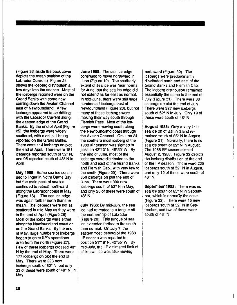
(Figure 33 inside the back cover June 1988: The sea ice edge northward (Figure 30). Thedepicts the mean position of the continued to move northward in icebergs were predominantlyLabrador Current.) Figure 24 June (Figure 19). The southerly distributed north and east of theshows the iceberg distribution a extent of sea ice was near normal Grand Banks and Flemish Cap.few days into the season. Most of for June, but the sea ice edge did The iceberg distribution remainedthe icebergs reported were on the not extend as far east as normal. essentially the same to the end ofGrand Banks with some now In mid-June, there were still large July (Figure 31). There were 80coming down the Avalon Channel numbers of icebergs east of icebergs on plot the end of July.east of Newfoundland. A few Newfoundland (Figure 28), but not There were 327 new icebergsicebergs appeared to be drifting many of these icebergs were south of 520 N in July. Only 19 ofwith the Labrador Current along making their way south through these were south of 480 N.the eastern edge of the Grand Flemish Pass. Most of the ice-Banks. By the end of April (Figure bergs were moving south along August 1988: Only a very little25), the icebergs were widely the Newfoundland coast through sea ice off of Baffin Island re-scattered, with most still being the Avalon Channel. On June 24, mained south of 650 N in Augustreported on the Grand Banks. the southern most iceberg of the (Figure 21). Normally, there is noThere were 114 icebergs on plot 1988 liP season was sighted in sea ice south of 650 N in August.the end of April. There were 151 position 42013 N, 46059* W. By The 1988 liP season closedicebergs reported south of 520 N, the end of June, most of the August 2, 1988. Figure 32 depictsand 95 reported south of 480 N in icebergs were distributed to the the iceberg distribution at the endApril. north and east of the Grand Banks of the lIP season. There were 225
and Flemish Cap., with very few to icebergs south of 520 N in August,May 1988: Some sea ice contin- the south (Figure 29). There were and only 10 of these were south ofued to linger in Notre Dame Bay, 356 icebergs on plot the end of 480 N.but the main pack of sea ice June. There were 300 newcontinued to retreat northward icebergs south of 520 N in May, September 1988: There was noalong the Labrador coast in May and only 20 of these were south of sea ice south of 650 N in Septem-(Figure 18). The sea ice edge 480 N. ber, which is normally the casewas again farther north than the (Figure 22). There were 15 newmean. The icebergs were not as July 1988: By mid-July, the sea icebergs south of 520 N in Sep-scattered in mid-May as they were ice had retreated to a tongue off tember, and two of these werein the end of April (Figure 26). the northern tip of Labrador south of 480 N.Most of the icebergs were either (Figure 20). This tongue of seaalong the Newfoundland coast or ice extended farther to the southon the Grand Banks. By the end than normal. On July 7, theof May, large numbers of icebergs easternmost iceberg of the 1988began to enter lIP's operations liP season was reported inarea from the north (Figure 27). position 51019' N, 42055' W. ByFew of these icebergs crossed 480 mid-July, the liP estimated limit ofN by the end of May. There were all known ice was also moving177 icebergs on plot the end ofMay. There were 223 newicebergs south of 520 N, but only33 of these were south of 480 N, inMay.
26

Figure 11.
65N 65W 60W 55W 50W 65N
Greenland
60N 60N
55N - 55N
50N O 50NSea Ice ConditionsOctober 14, 1987 New-
3/10 or greater sea( f_..n . _,,/?andice concentration --- • -- ••/,)•"
(Redrawn from Joint 4Ice Center, 1988)
1972-82 meansea ice edge
(Redrawn from Naval 45NOceanography Command, 1986)_
60W 55W 50W 45W
27

Figure 12.
65W 60W 55W 50W65N 65N
Greenland
60N 60W
55N 55N
Labrador
Sea Ice Conditions z .•d50N ,SO,,7-- 5 N
November 18,1987 New-3/10 or greater sea foundlandice concentration
(Redrawn from JointIce Center, 1988)
1972-82 meansea ice edge
(Redrawn from Naval 45NOceanography Command, 1986)
60W 55W 50W 45W
28

6N65W 60W 55W OWN
SGreenland
55N - 55N
Labrador
50N -SONSea Ice ConditionsDecemoer 16, 1987 New-3/10 or greater sea %tndlandice concentration -
(Redrawn from JointIce Center, 1988)
1972-82 meansea ice edge
(Reu awn from Naval 45NOceanography Command, 1986)
60W 55W 50W 45W
29

Figure 14.
65W 60W 55W 50W
65N 65N
Greenland
0 Q>
60N 60N
55N 55N
Labrador •
50N 5ONSea Ice Conditionst,9January 13, 1988 , New-3/10 or greater seai .- •• foundland•
ice concentration -'- v _..,.?,._.,.(Redrawn from Joint
Ice Center, 1988)
1972-82 meansea ice edge 4 5N
(Redrawn from NavalOceanography Command, 1986) _ !
60W 55W 50W 45W
30

Figure 15.
65N 65W 60W .55W 50W 65N
Greenland
60N 60N
55N 55N
Sea Ice edge ton
(Redrawn from Jonavt
Oceanography Command, 1986)
60W 55W 50W 45W
31


Figure 17.
6N65W 60W 551W 50W65
Greenland
60N 60N
55N 55N
5ON SON
Apile Ce0, 1988)Ne
1972-82 meansea ice edge45
(Redrawn from Naval45Oceanography command, 1986)
60W 55W 50W 45W
33

Figure 18.
65N 65W 60W 55W 50W 65N
Greenland
60N 60N
55N 55N
Labrador ..
50N 50NSea Ice Conditions
May 18, 1988 New-3/10 or greater sea fondanice concentration - - -- •-7,-.'f•
(Redrawn from JointIce Center, 1988)
1972-82 meansea ice edge
(Redrawn from Naval 45NOceanography Command, 1986)
60W 55W 50W 45W
34

Figure 19.
65N 65W 60W 55W 50W 65N
Greenland
60N 60N
55N 55N
Labrador
Sea Ice Conditions i '
June 15, 1988 ew3/10 or greater sea foun-anice concentration
(Redrawn from JointIce Center, 1988)
1972-82 meansea ice edge 45N
(Redrawn from NavalOceanography Command, 1986) __ _
60W 55W 50W 45W
35

Figure 20.
65N 65W 60W 55W 50W65N 65N:
: Greenland
60N 60N
55N 55N
Labrador
50N 5ONSea Ice Conditions i -'
July 13, 1988, New3/10 or greater seaC _.. ,2/,foundlandice concentration "- -" - --- _•_.--
(Redrawn from Joint
Ice Center, 1988)
1972-82 meansea ice edge
(Redrawn from Naval 45NOceanography Command, 1986)
60W 55W 50W 45W
36

Figure 21.
65N 65W 60W 55W 50W 65N
Greenland
60N 60N
55N 55N
Labrado
5ON 5ON
(Redrawn from Joint
Ice Center, 1988)
1972-82 meansea ice edge
(Redrawn from Naval 45NOceanography Command, 1986)
60W 55W 50W 45W
37

Figure 22.
65N 65W 60W 55W 50W65 65N
Greenland
60N 60N
55N 55N
50N 5ON
ice concentration"i -"an'
(Redrawn from Joint
Ice Center, 1988)
1972-82 meansea ice edge 45N
(Redrawn from NavalOceanography Command, 1986)
60W 55W 50W 45W
38
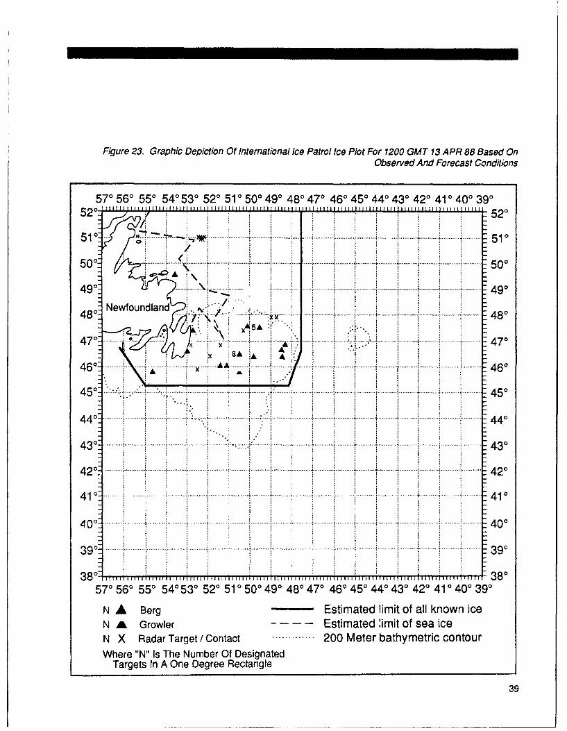
Figure 23. Graphic Depiction Of International Ice Patrol Ice Plot For 1200 GMT 13 APR 88 Based OnObserved And Forecast Conditions
570 560 550 540 530 520 510 500 490 480 470 460 450 440 430 420 410 400 390
520: - 520
A
490- -..-..490
0-Newfoundland/480 480
470 r 4708AA
t( B A A. .
460 460
450 .... ...... 450
440 440
430 430
42....... 420....
430
390. 390
570 560 550 540 530 520 51 0500 490 480 470 460 450 440 430 420 4104300390
N A Berg - Estimated limit of all known iceN A Growler - -- Estimated :imit of sea iceN X Radar Target/I Contact ....200 Meter bathymetric contourWhere "N" Is The Number Of Designated
Targets In A One Degree Rectangle
39

Figure 24. Graphic Depiction Of International Ice Patrol Ice Plot For 1200 GMT 15 APR 88 Based OnObserved And Forecast Conditions
570 560 550 540530 520 510 500 490 480 470 460 450 440 430 420 410 400 390
520. 1111111 t I i llIII I I
50 5200
4 0 Newfound .la ..d.. 480...........
470 .... . 47
4600
045
430 430
410 410
40 40
390 39 A40
38 1I ~~rr-r-r II ,~r~rnTr-r¶TrnA8
Tagt nA One Dere Rcanl
40
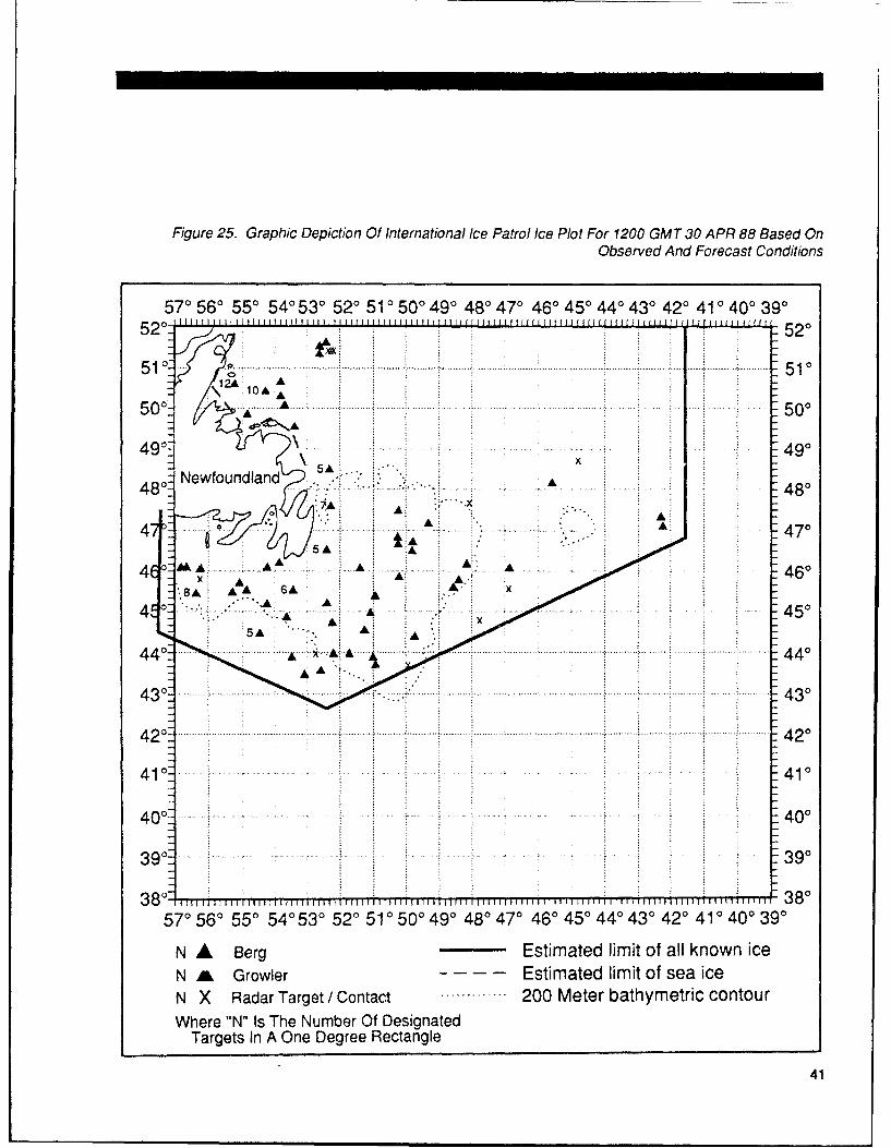
Figure 25. Graphic Depiction Of International Ice Patrol Ice Plot For 1200 GMT 30 APR 88 Based OnObserved And Forecast Conditions
570 560 550 540 530 520 51 0 500 490 480 470 460 450 440 430 420 410, 400 390
515112A AA
10~A AA
490 490
5SA z40Newfoundland -. , 8
0~ A A
AA A
4 Q .1- .:-1...ý,".-i 1 4 7 '
390 .... A . A':39
380A 3840
NA A Grwe -45-Etmae0ii o e c
4T 41

Figure 26. Graphic Depiction Of International Ice Patrol Ice Plot For 1200 GMT 15 MA Y88 Based OnObserved And Forecast Conditions
570 560 550 540 530 520 51 0500 490 480 470 460 450 440 430 420 41 0 400 390
520--I It~ I 520
51t 510A
17 A:
500 50'
490 49'
AA
40~ *. -470
A 7A0 A
A 46'
450 A0450
440......-440
40-43 430
42'
410: -,-- .. 410
390': 390
380 1 11 1 r'I-t 1 1- M illt~rr~ ri I ?Tt III II f It 114 11 11 III 11111fIl l]IIt Itr~ rrrr lilt II111 I I IT I ] i[ 1rT1rrr1--1 38570 560 550 540530 520 510 500 490 480 470 460 450 440 430 420 410 400 390
N A Berg Estimated limit of all known iceN AL Growler ---- Estimated limit of sea iceN X Radar Target / Contact 200 Meter bathymetric contourWhere "N" Is The Number Of Designated
Targets In A One Degree Rectangle
42

Figure 27. Graphic Oeptct 3n Of L7:wmabona! Ice Patrol Ie Po For ?200 GMT3O MAY 8.6 Based OnObserved And Fotecast Condatons
570 56& 55° 54' 53`ý 52 51 50' 49- 48" 47' 46" 45' 44'- 43" 42° 41 0 401 39052"52<
8 •A 6A -o84
510 £ 510A A 14A 5A S A.
0 "A - A9AA
49A A
490 -6A At49
Newfoundland • : 48A4848
4 [ o 0, . 4 7 r,
121A
46 A% A A 46045A• 4
45-
440 44'
430 43'
420 42Z
410• 41
0 400
39o 390
380 i T 380570 56° 550 540530 520 510 50T 49" 480 470 460 450 44° 43° 42° 41' 40° 390
N A Berg . Estimated imit of all known iceN A Growler Estimated limit of sea iceN X Radar Target I Contact 200 Meter bathymetric contourWhere "N" Is The Number Of Designated
Targets In A One Degree Rectangle
43

Figure 28. Graphic Depiction Of International Ice Patrol Ice Plot For 1200 GMT 15 JUN 88 Based OnObserved And Forecast Conditions
570 560 550 540530 520 510 500 490 480 470 460 45" 440 430 420 410 400 390
520 5206A 24A 9A
6 x 1 A A5 1 0 o / ....... A 5 1
lA 15k A 16A 20A 25A 12A 6A5 0 0 - AL A 4l
500A' AAA 15 249, 12 A4
d . 1 3 A , A A A4
480 o Newfoundland 5A 12" A A480
A. 480
A x
47 -- - " 47 '" '" o~~ A -X . "
46 ° A&AL 460
4 o- %:. x450
440 - ! -440
430 - 4304 2 °: 0 ...... ................. . .... . . .. ..... . . . . .. 4 °420 42'
410 41'
40 ° - 4 0
390 39038 7 °- ri
38 o3 0 | ! I J I I II Illllltll ll i t I t lI I l I lill I I I1 I| 11 t I | I I Ip I1 illl | |] I ' I I I 38I570 560 550 540530 520 510 500 490 480 470 460 450 44" 430 420 41 0 400 390
N A Berg - Estimated limit of all known ice
N A Growler Estimated limit of sea iceN• X Radar Target / Contact ........ 200 Meter bathymetric contour
Where "N" Is The Number Of DesignatedTargets In A One Degree Rectangle
44

Figure 29. Graphic Depiction Of International Ice Patrol Ice Plot For 1200 GMT 30 JUN 88 Based On,Observed And Forecast Conditions
570 560 550 540530 520 510 500 490 480 470 460 450 440 430 420 410 400 390
5 il0 Il I I I f I IIIH 11 ) 11 1 lI I II I IJ .J.L .J..I III ..J. 11 1 1 1 1 1 1 1 11 1 1 1[1I [ III ItI 'J.J.IJ.' II li.U..I~ IIII.. 4 J....J4... J 5 0A;*
:6A 6A 26 :A*
5 1 0c . ............ ... .... ..... ... .................. ... 5 1 0t5k 10A 8A 7A ý31k 18k k
50 50
7A A8A
AA470..... ... .. 470..
4 9... A ý ... ...... ...... ... ........ 9460A 46
4 0 4Q
390 A, 390
50 5050503 2 1509 8 7040404f 3 2 1 Q 9
5 -- 450
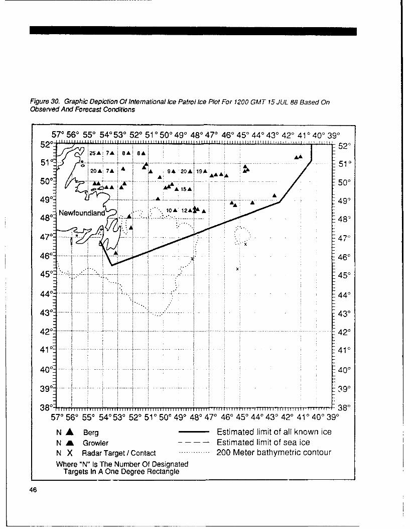
Figure 30. Graphic Depiction Of International Ice Patrol Ice Plot For 1200 GMT 15 JUL 88 Based OnObserved And Forecast Conditions
570 560 550 540 530 520 51 0 500 490 480 470 460 450 440 430 420 41 0 400 390
520:1J.LL.LJ...J.L±J 520ý25A: 7A 8A; SA:h
A AA
A
480 New o.nlan.. . ......... ......... 48...
450 .4500
4Q A. . .: .....
390 ...... ..... .... 490
N8: 48rwe simtdlmto e c
460

Figure 31. Graphic Depiction Of International Ice Patrol Ice Plot For 1200 GMT 30 JUL 88 Based OnObserved And Forecast Conditions
570 560 550 540 530 520 51 0 500 490 480 470 460 450 440 430 420 41 0 400 390
520 1 HIIII H LLLL~jLL LL..JLJJIj.I .. L LJ L.U H I II I!I II I fIil11 11111111111It I L IIJ-.14I~ JI I I I.! LL UIU& 5 0
7A aA M
510c:.................................. ......A............... .......... .......... ........... 51
AA A A& 4 A5Q0 .... .... 500
A
490 490
6A A AS40Newfoundland -~ 4 A A5 8
0 X A
470 470
440.- 440
420. 420
40- 400
390- - 390
38 0 71 -r 14 1 11 11 11 1r**'- 111~ r1 r-ir I ITr II I I f r~' I *I~i~ I I~ri, I r~I ' I I 1 380570 560 550 540530 520 510 500 490 480 470 460 450 440 430 420 410 400 390
N A Berg - Estimated limit of all known iceN A Growler ---- Estimated limit of sea iceN X Radar Target /Contact 200 Meter bathymetric contourWhere "N" Is The Number Of Designated
Targets In A One Degree Rectangle47

Figure 32. Graphic Depiction Of International Ice Patrol Ice Plot For 1200 GMT 02 AUG 88 Based OnObserved And Forecast Conditions
570 560 550 540530 520 510 500 490 480 470 460 450 440 430 420 410 400 390
52- -'''''''JL..UI.~.l.U ~~52015A: 33A: 29A 26A: 6A
:7A 9A :ýAl
A AA
A A9 b
40Newfoundland AAA48480 A -480
470 -0470
46o -460
450-...... 450
440: ..... 440....
430 : 430
42~ 42'
410: . 410
390: -.-. 390
380 1 ITTII~'I1 I~I~ ~ '~'rr'~ IfIIIIIII I I I Ii Ii Ii I7' 1?I Ii I I Ii I I I I IF I Ii I I II II T*~*TI * I- 38~570 560 550 540 530 520 51 0500 490 480 470 460 450 440 430 420 41 0 400 390
N A Berg Estimated limit of all known iceN AL Growler --- - Estimated limit of sea iceN X Radar Target / Contact --..... 200 Meter bathymetric contourWhere "N" Is The Number Of Designated
Targets In A One Degree Rectangle
48

Discussion of Ice andEnvironmental Conditions
The number of icebergs that pass eventually reach open water Beginning in April and continuingsouth of 48"N in the International unless grounded. The melting of through August, large numbers ofIce Patrol area each year is the sea ice itself is affected by snow icebergs began to drift south ofmeasure by which International cover (which slows melting) and 520 N and enter lIP's area. ThereIce Patrol has judged the severity air and sea water temperatures. was a good supply of icebergsof each year since 1913. The As sea ice melt accelerates in the available to drift south of 480 Naverage number of icebergs spring and early summer, trapped from April to August, but thedrifting south of 480 N from 1913 icebergs are rapidly released and environmental and oceanographicto 1987 is 395 (Alfultis, 1987). then become subject to normal conditions were not favorable forWith 187 icebergs south of 480 N, transport and deterioration, the southward drift of icebergs.the 1988 ice year was less severe Most of these icebergs did not driftthan the 1913-1987 average. The Labrador Current, aided by south with the Labrador Current to
northwesterly winds in winter, is the Tail of the Grand Banks, butSince the number of icebergs the main mechanism transporting drifted east. By July and August,calved each year by Greenland's icebergs south to the Grand iceberg deterioration became aglaciers is in excess of 10,000 Banks. In addition to transporting major factor preventing icebergs(Knutson and Neill, 1978), a icebergs south, the relatively cold from surviving a drift south of 480sufficient number of icebergs exist waters of the Labrador current N. In summary, it appears thein Baffin Bay during any year. keep the deterioration of icebergs environmental and oceanographicTherefore, annual fluctuations in in transit to a minimum, conditions set up an unfavorablethe generation of Arctic icebergs is eastward drift, preventing the largenot a significant factor in the The 1988 International Ice Patrol number of icebergs entering lIP'snumber of icebergs passing south season did not open until mid-April area from drifting soutt of 480 Nof 48' N annually. The factors that because of the small number of with the Labrador Current.determine the number of icebergs icebergs drifting south of 520 orpassing south of 48'N each 480 N in January, February, andseason are the supply of icebergs March. With the sea ice notavailable to drift south onto the extending as far south as normalGrand Banks, those affecting in February and March, theiceberg transport (currents, winds, icebergs were not protected asand sea ice), and those affecting long from deterioration. Thethe rate of iceberg deterioration below average sea ice conditions(wave action, sea surface tem- at the beginning of the seasonperature, and sea ice). would normally lead to a relatively
light ice season with a late start.Sea ice acts to impede the trars-port of icebergs by winds andcurrents and also protects ice-bergs from wave action, the majoragent of iceberg deterioration.Although it slows current and windtransport of icebergs, sea ice isitself an active medium, for it iscontinually moving toward the iceedge where melt occurs. There-fore, icebergs in sea ice will
49

References
Alfultis, M.A., Iceberg Populations South of 48 N Since 1900, Report ofthe International Ice Patrol in the North Atlantic,1987 Season, CG-188-42, U.S. Coast Guard, Washington D.C., 1987.
Anderson, I. Iceberg Deterioration Model, Report of the InternationalIce Patrol in the North Atlantic, 1983 Season, CG-188-38, U.S. CoastGuard, Washington D.C., 1983.
Atmospheric Environment Service (AES), Thirty Day Ice Forecast forNorthern Canadian Waters, December 1987 to April 1988.
Hanson, W.E., Operational Forecasting Concerns Regarding IcebergDeterioration, Report of the International Ice Patrol in the North Atlantic,1987 Season, CG-188-42, U.S. Coast Guard, Washington D.C., 1987.
Knutson, K.N. and T.J. Neill, Report of the International Ice PatrolService in the North Atlantic Ocean for the 1977 Season, CG-188-32,U.S. Coast Guard, Washington D.C., 1978.
Mariners Weather Log, Spring 1988, Vol. 32, Number 2, 1988a.
Mariners Weather Log, Summer 1988, Vol. 32, Number 3, 1988b.
Mariners Weather Log, Fall 1988, Vol 32, Number 4, 1988c.
Mariners Weather Log, Winter 1989, Vol. 33, Number 1, 1989.
Murphy, D.L. and I. Anderson. Evaluation of the International Ice PatrolDrift Model, Report of the International Ice Patrol in the North Atlantic,1985 Season, CG-188-40, U.S. Coast Guard, Washington D.C., 1985.
Naval Oceanography Command, Sea Ice Climatic Atlas: Volume IIArctic East, 1986.
Navy-NOAA Joint Ice Center, Naval Polar Oceanography Center,Southern Ice Limit, Published Bi-monthly, 1988.
50

Acknowledgements
Commander, International Ice Patrol acknowledges the assis-tance and information provided by the Atmospheric EnvironmentService of Environment Canada, U.S. Naval Fleet Numerical Oceanog-raphy Center, U.S. Naval Eastern Oceanography Center, and the U.S.Coast Guard Research and Development Center.
We extend our sincere appreciation to the staffs of the Cana-dian Coast Guard Radio Station St. John's, Newfoundland/VON, IceOperation St John's, Newfoundland, Air Traffic Control Gander, New-foundland, Canadian Forces Gander and St John's, Newfoundland, andthe Gander Weather Office, and to the personnel of U.S. Coast GuardAir Station Elizabeth City, U.S. Coast Guard Air Station Cape Cod, U.S.Coast Guard Communications Station Boston, and USCGC NORTH-WIND, for their excellent support during the 1988 International Ice Patrolseason.
It is also important to recognize the efforts of the personnel atthe International Ice Patrol: CDR S. R. Osmer, LCDR W. A. Hanson,Dr. D. L. Murphy, LCDR R.L. Tuxhorn, LT N. B. Thayer, LT M. A.Atfultis, MSTCS G. F. Wright, MSTC M. F. Alles, YN1 P. G. Thibodeau,MST1 M. G. Barrett, MST1 C. R. Moberg, MST2 J. L. Perdue, MST2 J.R. Shubert, MST2 D. D. Beebe, MST2 D. A. Hutchinson, MST2 J. C.Myers, MST3 M. E. Petrick, MST3 P. B. Reilley, MST3 R. C. Lenfen-stey, MST3 N. A. Capobianco, MST3 M. D. Baechler, and MST3 C. F.Weiller.
51

Appendix AList of Participating Vessels, 1988
ICEVESSEL NAME FLAG SST REPORTSABITIBI CLARBORNE FED. REP. OF GERMANY 9ABITIBI CONCORD FED. REP. OF GERMANY 8ABITIBI MACADO FED. REP. OF GERMANY 4ABITIBI ORINOCO FED. REP. OF GERMANY 3ADA GORTHON SWEDEN .1ADITYA KIRAN INDIA 1AIGIANIS ES3AILSA LIBERIA 2ALBRIGHT PIONEER UNITED KINGDOM IALCYONE FRANCE 1ALFRED NEEDLER CANADA 1ALMARE TERZA ITALY 5 1ALTA LIBERIA IALUK DENMARK 1ANDROMEDA POLAND .ANN HARVEY CANADA 6ANNA ::ST. VINCENT AND THE GRENADINES 7'APILIOTIS GREE 1ARC MINOS GRECE IARCTIC CANADA 1ARIES CYPRUS ::ATLANTIC AMITY UNITED KINGDOM 1ATLANTIC CARTIER FRANCE 1ATLANTIC CONVEYOR UNITED KINGDOM 2ATLANTIC OLGA CANADA IATLANTIC QUEEN U. S. A. 2AVALON HARVESTER UNKN•.N 1BAFFIN CANADA 1BAKKAFOSS BAHAMAS 4BALTIC CYPRUS 2BARDU NORWAY 2BELLE ISLE FRANCE 1BENIER UNKNOWN I1BENNY SKOU DENMARK 1
BEVERLYFAYE CANADA .1SST = SEA SURFACE TEMPERATURE
53

Appendix A
ICE
VESSEL NAME FLAG SST REPORTS
BIJELO POUE YUGOSLAVIA I
BLUE BIRD FED. REP. OF GERMANY 1
DOESEA PANAMA 1
BONAVISTA BAY CANADA 4
BOWDRILL 3 CANADA 4
BRAE TRADER LIBERIA 1
BRIDGEWATER. FED. REP. OF GERMANY 2
BRITISH STEEL UNITED KINGDOM 2
CANADIAN EXPLORER UNITED KINGDOM 5
CANMAR AMBASSADOR UNITED KINGDOM 14
CANMAR EUROPE. BELGIUM 16
CANMAR SPIRIT PANAMA 2
CAPEROGER CANADA 5
CAPE SOUNION GFEECE 1
CARIAEN SWEDEN 1CAST CARIBOU LIBERIA 7 2
CAST HUSKY: BAHAMAS 3 7
CAST MUSKOX BAHAMAS 3
CAST OTTER BAHAMAS 2
CAST POLARBEAR LIBERIA 2
CAVALLO .CANADA 3
CECELIEA DESGAGNES CANADA 1
CHARLOTTE BASTIAN FED. REP. OF GERMANY 2
CHESAPEAKE BAY U.S.A. 1
CHIMO UNITED KINGDOM 5 4
CHIPPEWA LIBERIA 1
CICERO CANADA 1
COLORADO U.S.A. 3 3
COMMANDANT GUE FRANCE 1
COMPANION EXPRESS SWEDEN 2
DART ATLANTIC LIBERIA 1
DELPHINUS ITALY 7 9
DES CHESNES UNKNOWN 1
DISKO DENMARK 1
DODSLANDE LIBERIA 2 6
54

Appendix A
ICEVESSEL NAME FLAG SST REPORTS
DUKE OF TOPSAIL UNITED KiNGDOM' 1DUSSELDORF EXPRESS FED. REP. OF GERMANY 1EASTERNTRADER PEOPLES REP. OF CHINA 18 5EASTERi,4 UNICORN PANAMA 1ENERCHEMFUSON CANADA 2ESTE SUBMERGER FED. REP. OF GERMANY 2EVERGOIN PANA1EXXON SAN FRANCISCO U. S. A. 1FALCON NORWAY 3FALMOUTH GRECE 1
FAROHARSON UNKNO .ffmJ 10 7FATIMA C PANAMA 10 11FEDERALDANUBE CYPRUS 3FEDERAL ELBE LIBERIA 1FEDERAL MMSA CYPRUS 4 4FEDERAL OTTAWA BELGIUM 3FIEDERALSAGUENAY LIBERIA 2FEDERAL SCHELDE LIBERIA 1FEDERAL ST CLAIR LIBERIA ;4FEDERAL THAMES CYPRUS 3
FER:.EUSE CANADA 2FIGARO CYPRUS 5FINNFIGHTER FINLAND 3
FINNPOLARIS FINLAND 5 3FLYING DART CANADA 1FOGO ISLE CANADA 1FRITHJOF FED. REP. OF GERMANY IFULLNESS LIBERIA 2
FURIA LIBERIA 1
GABARUS BAY CANADA 6
GATTINEAU UNKNOWN 1GRAND BARON CANADA 1
GRETE THERLSA DENMARK 8
GULF GRAIN LIBERIA 7 7
HARITAS CYPRUS 555

Appendix A
ICE
VESSEL NAME FLAG SST REPORTS
HARP CANADA 9
HELENA OLDENDORFF PANAMA 2
HERCE GOVINA YUGOSLAVIA 7
HOFJOKULL ICELAND 2
HOLCAN MAAS GREECE 1 3HOLCAN RIJN CYPRUS 7
CANADA 1
HUDSON CANADA 6
-YPHESTOS GREE:1ICE FLOWER DENMARK 3
ICE PEARL: DENMARK 6
ICEBLINK DENMARK 8
IMPERIAL BEDFORD ..:CANADA 1IMPERIAL ST CLAIRE CANADA 1
IRONMASTER PANAMA 5IRONBRIDGE UNITED KINGDOM 1
IROQUOIS PHILIPPINES. I
IRVING NORDIC CANADA 5
IRVING OURS POLAIRE CANADA 7
J.C. PHILLIPS CANAOA 1
JACKMAN CANADA 5
JACUHY BRAZIL 1
JOHGORTSON SWEDEN 2"JOHAN PETERSEN DENMARK 8
JOHANNA KRISTINA GREENLAND 6
JOHN CABOT CANADA 5
KAETHE HUSMANN FED. REP. OF GERMANY 1
KANGUK CANADA 2
KAREN WINTHER DENMARK IKAZIMIERZ PULASKI POLAND 2
KHUDOZHNIK REPIN U. S. S. R. 3
KOMSOMOLETS ESTONII U.S.S.R. 1
KONGAR INTREPID OFEECE 2
KUNUNGUAK DENMARK 3
LA CHESNAIS FRANCE 4
56

Appendix A
ICEVESSEL NAME FLAG SST REPORTS
LA PLATA MARUL CUBA 1LA RICHARDIAS FRANCE 6LACKENBY UNITED KINGDOM 5LE SAULE CANADA 1LEGER CANADA 1LEONARD J COWLEY CANADA 10LIEPAYA U.S.S.R. 1LONE VENTURE UNKNOWN 1LUGANO SWITZERLAND 1LUNNI FINLAND 10LYNCH U.S.A. 3 4MADZY SWEDEN 1MAGNUSJENSEN DENMARK 7MALINSKA YUGOSLAVIA 5MALOJA 2 SWITZERLAND 6MALVINA CYPRUS 1MANCHESTERCH NGER Cý UNITED KINGDOM 4MARGARITA CANADA 2MARIA GORTHON SWEDEN 1MARINE PACKER. CANADA 1MARKA L GRECE 1MAXWELL CANADA 1MELA PANAMA 1MIHALIS GREE CMINERVA LIBERIA 1NAJA ITTUK DENMARK 8NATHALIE DON II UNKNOWN 1NATSEK GREENLAND 1NAUTICAL ENTERPRISE UNKNOWN 1NAVIOS VALOR LIBERIA 2NEDLLOYD HUDSON U.S.A. 1NEPTUNE PERIDOT SINGAPORE 4NEW INDEPENDENCE LIBERIA 1NEWFOUNDLAND FALCON CANADA 2NIKKI ITTUK DENMARK 15
57

AppondIX A
ICE
VESSEL NAME FLAG SST REPORTS
NIN YUGOSLAVIA 2
NIVI ITT"'K DENMARK 9
NORDIC SUN LIBERIA 3
NORLANDIA FED. REP OF GERMANY 10
NORT-ERN CHERRY POLAND I
NORTHERN EXPRESS NETHERLANDS 3
NORTHWND U. S. A. 14 15
NOSIRA SHARON UNITED KINGDOM 1
NUKA ITTUK DENMARK 7
NUNGU ITTUK DENMARK 2 20
NURNBERG ATLANTIC FED. REP. OF GERMANY 1
OCEAN TRAVELLER SINGAPORE 3
OLYMPIC MERIT PANAMA 2
ONTADOC CANADA 2
PACIFIC CONFIDENCE PANAMA 1
PACIFIC EXPRESS LIBERIA 1
PACIFIC PRESTIGE UNITED KINGDOM 1
PACIFIC PROMINENCE UNITED KINGDOM I
PAN MAPLE GFCE 1
PETKA YUGOSLAVIA 5 4
PETROLAB CANADA 4
PLACENTIA BAY CANADA 2
PLANET BAHAMAS 1 3
PONTE DE CORSEN FRANCE 1
POLAR NANOQ DENMARK 5
POLY CRUSADOR NORWAY 1
POLY SUNRISE NORWAY 1
POMORZE ZACHOONIE POLAND 2
PROJECT ORIENT NETHERLANDS ANTILLES 3
PUMA JAPAN 7
QUEEN ELIZABETH I1 UNITED KINGDOM 1 1
RADNIK PANAMA 1
RAVENNA PANAMA 6
RE•oP'r MAERSK DENMARK 2 2
ROSS R CANADA 1
58

Appendix A
ICE
VESSEL NAME FLAG SST REPORTS
SAINT CONSTANTINOS LIBERIA 6
SAINT LAURENT PANAMA 1
SAINT LUCIA LIBERIA 2
SANO R DENMARK I
SANTAN PHILIPPINES 3 1
SASKETCHEWAN PIONEER CANADA 1
SAULE NO 1 U.S.S. R. 1
SEA HAWK U.S.A. 1
SEALAND CONSUMER U. S. A. 1 1
SEDCO 710 CANADA 2
SELKIRK SETTLER CANADA 2
SIR JOHN FRANKLIN CANADA 1 1
SIR ROBERT BOND CANADA 1
SIR WILFRED GRENFELL CANADA 4
SKEENA UNITED KINGDOM 3 2
SKIDEGATE CANADA 1
SLETHAV NORWAY 1
SPRAY TANAO PHILIPPINES 1
SPRAYNES PANAMA 5 2
STOLT ASPIRATION PANAMA 2
STOLT BOEL LIBERIA 1
STOLT CROWN LIBERIA 2
STRAITS PRIDE SINGAPORE 1
STRATHCONAN UNITED KINGDOM 1
SVANUR ICELAND 1
TADEUSZ KOSCIUSZKO POLAND 2
TAURIA CYPRUS 1
TEVERA CYPRUS 4
TEXACO WESTMINISTER UNITED KINGDOM 3
TEXAS CLIPPER U.S.A. 3
THEOGENNITOR CYPRUS I
TNT EXPRESS AUSTRALIA 1
TOK)ACHI MARU JAPAN 4 4
TORM GUNHILD DENMARK 4
TORNADO POLAND 159

Appendix A
ICEVESSEL NAME FLAG SST REPORTS
TO-.. BERMUDA 1TOSA MARU JAPAN 2
TACK.ER 1 CANADA 1TRIUMPH SEA CANADA 7VAIR CANADA 1VARJAKKA BAHAMAS 1VICTOR BUGAEV U. S. S. R. 1VIGILANT UNITED KINGDOM 1 1VISHA PARIJAT. .INDIA 2 3VROUWE JOHANNA NETHERLANDS 1 5WHITE SEA SINGAPORE 1
WILFRED TEMPLEMAN CANADA 1
ZAMBESI CANADA 1ZANDBERG CANADA 5ZEILA. CANADA 1ZEVEN CANADA 1
ZiEMIA SUWALSKA POLAND 1ZONNEMARIE CANADA 2
60

Appendix BInternational Ice Patrol's 1988 Drifting Buoy Program
Donald L. Murphy
INTRODUCTION The 1988 drifting buoy program temperature sensor mountedwas unique in two ways. First, it approximately 1 m below the
The 1988 iceberg season was the marked the first time that all of the waterline, a drogue tensionthirteenth consecutive year that operational buoys were recovered monitor, and a battery voltagethe International Ice Patrol (liP) and returned to Ice Patrol at the monitor. The sea surface tem-has used satellite-tracked buoys to conclusion of the season. Sec- perature is accurate to approxi-measure currents in its operations ond, it was the first time that Ice mately 10C.area in the western North Atlantic Patrol deployed mini-drifting buoysOcean. The buoy trajectories are during its season. In all, Ice Patrol The data from the buoys areused to provide near realtime reconnaissance aircraft deployed acquired and processed bycurrent data to the Ice Patrol five mini-drifters, four in coopera- Service ARGOS. Ice Patroliceberg drift model. These tion with the U.S. Navy and one queries the ARGOS data files andcurrents are used to modify the with the Canadian Atmospheric stores the buoy data once daily.mean currents temporarily in the Environment Service (AES). Most of the buoy position data fallregion through which the buoy is within the standard accuracymoving. Shortly after a buoy The standard configuration for the provided by Service ARGOSdeparts the regior, the current operational buoys is a 3 meter (-350 m). All of the buoy datareverts to its mean value, long spar hull with a 1 meter were entered onto the Global
diameter flotation collar. Each Telecommunications SystemDuring 1988 Ice Patrol deployed buoy was equipped with a 2 by 10 (GTS). Each buoy is assigned aeleven buoys, six for operational meter window-shade drogue World Meteorological Organizationuse and five as part of an evalu- attached to the buoy with a 50 (WMO) number.ation of a new buoy type. Of the meter tether of 1/2" (1.3 cm)six operational buoys, five pro- nylon. The center of the drogue Table B-1 summarizes the 1988vided excellent data. One buoy was at a nominal depth of 58 m. buoy deployments.failed on deployment. In addition, each buoy had a
Table B- 1. Summary of 1988 Deployments.
ARGOS WMO DEPLOYMENT DEPLOYMENT RECOVERY
ID I D DATE POSITION DATE
4530 44501 15 APR (106) 51-59N 52-00W 16 JUN (168)
4540 44502 15 APR (106) 49-59N 50-30W 17 JUN (169)
4558 44503 30 APR (121) 46-59N 47-19W 21 JUN (173)
4563 44504 19 MAY (140) 53-OON 52-05W 16 JUN (168)
4564 None Assigned 5 JUN (157) 52-OON 52-OOW FAILED ON DEPLOYMENT
4566 44505 1 AUG (214) 59-01N 61-26W 27 OCT (301)
61

BUOY DEPLOYMENT Several of the study's conclusions eddy scales. This is a sound rec-STRATEGY and recommendations support Ice ommendation. Ice Patrol deploys
Patrol's recent deployment buoys near drifting icebergs onlyA recent study (FENCO,1987), strategies with the intent of gaining for specific iceberg drift studies,sponsored by the AES, devised the most benefit from a few buoys. not for operations.strategies for the optimum deploy- A fundamental conclusion of thement strategy for drifting buoys study is to deploy buoys as far Finally, the study recommends aused to derive oceanic currents for north (north of 50N) as possible thorough review of the Ice Patroliceberg drift forecasting. This because the southward mean flow mean current file and the inclusionstudy focused on Canadian of the Labrador Current will carry of data on the variability of thedomestic iceberg interests, that is, the buoys into the southern areas current. Ice Patrol has begunon regions where offshore oil of interest. Ice Patrol's experience such a review and is using driftexploration is taking place (the has shown that this approach is tracks collected since the begin-slope and shelf east of Newfound- reasonable with two important ning of the buoy program (1976) toland and Labrador). Although the limitations. The first is that early in improve the mean current data.area of Ice Patrol operations the iceberg season (March andextends far to the south of this April) the buoys should not be de- AIRCRAFT DEPLOYMENTSregion, many of the study results ployed in areas with significantapply directly to the lIP mission. concentrations of sea ice ( > 3/10) Ice Patrol has deployed satellite-
so that wind-driven movement of tracked buoys from HC-130'sThe study showed that, even for a the sea ice will not contaminate since 1979. The buoy is strappedsmall portion of the region (250 km the drifter data. Second, in many into an air-deployment packagex 250 km), at least 400 buoys cases buoys deployed from 50 - and launched out the rear door ofwould be required to resolve the 520N move eastward to the north an HC-130 flying at an altitude ofeddy field throughout the iceberg of Flemish Cap, and hence do not 500 feet (150 m) at 150 knots (77season. Ice Patrol's operations enter the region south of Flemish mis). The air-deployment pack-area is many times this size. The Pass. Because Ice Patrol requires age consists of a wooden palletcosts associated with deploying drift data in this area, it is fre- and a parachute, both of whichand tracking many hundreds of quently necessary to deploy buoys separate from the buoy after itbuoys far exceeds the entire Ice directly in the pass to ensure that enters the water. The parachutePatrol budget. Thus, such cover- the buoy will move to the south. In riser is cut by a cable-cutter that isage is impractical. this case the buoys are deployed activated by a battery that ener-
at 470N between 46-30OW and 47- gizes when immersed in saltIce Patrol's buoy deployment 300W. water. The pallet separates whenstrategy focuses on the current salt tablets dissolve and releasethat is the major conduit of ice- The study recommends against straps holding the buoy to thebergs into the North Atlantic releasing a buoy beside a particu- pallet. The buoy then floats freeshipping lanes, the southward- lar iceberg because, in a period of and the drogue falls free andflowing off-shore branch of the a few days, the buoy and the unfurls.Labrador Current. The goal is to iceberg are likely to be separatedmonitor this current for the entire by distances larger than the typicalseason by keeping one or twobuoys in it at all times.
62

The air-deployment package failed The error-free position data are BUOY TRAJECTORIESin half (3 of 6) of the 1988 then fitted to a cubic spline curvelaunches. The failures were to arrive at an evenly-spaced In the following sections eachsimilar in that the wooden pallet record with an interval of three buoy trajectory is discussedthat holds the buoy and drogue hours. This process results in a separately, presented in chrono-together broke apart when it slight reduction in the number of logical order by buoy deploymententered the HC- 30's airstream. fixes per day (from 10 to 8). Next, date. Only the operational buoysIn all cases the parachute oper- the position records are filtered are discussed.ated property and the buoys using a low-pass cosine filter withdescended to the surface at a a cut-off of 1.16 x 10⁻⁵ Hz (one The intent of the following discus-normal speed. Two of the buoys cycle per day). This filter removes sions is to summarize each buoy's(4563 and 4566) transmitted most tidal and inertial effects. performance and the data that itnormally, but one (4564) failed to Finally, the buoy drift speeds are contributed to Ice Patrol opera-"transmit after its deployment. It is calculated at three-hour intervals tions. It is not intended to be annot certain that the buoy failure using a two-point backward differ- exhaustive date. analysis. Thewas due solely to the failure of the encing scheme. buoy data from the area east ofdrop package. In most cases the 390W, the eastern boundary of thebuoy survives and the most Most of the trajectory plots pre- Ice Patrol operations area, are notserious result is that the parachute sented in this report are from the presented. All of the data from theremains attached to the buoy hull. filtered records. Also presented lIP drifting buoy program areWhen this happens the parachute for each buoy is a plot of the time archived at the lIP office in Groton,can act as a near-surface drogue history of the U (east is positive) Connecticut.until it collapses and entangles and V (north is positive) compo-with the buoy hull or drogue tether. nents of velocity from the filtered
records. Finally, a time history ofDATA PROCESSING the raw sea surface temperature
data is plotted for each buoy. TheAlthough the raw position and dates used in all of the plots aretemperature data are relatively year-dates, which are numberednoise free, all records are scanned sequentially starting at 1 onbefore processing to ensure January 1. In the text, the year-quality control. First, duplicate dates are included parenthetically.positions and positions with timeseparations of 30 minutes or lessare deleted. Then, positions <700 m from adjacent positions aredeleted, unless the deletion resultsin a time separation of four ormore hours.
63

18 rr. 16t
o) 14
12-
10-
Buoy 4530 r (-
CE
Buoy 4530 (Figure B-1) was • Fdeployed at 1622Z on 15 April 2 -(106) at 51-59N, 52-00W. It o -
provided uninterrupted data until -2_ I , i...its recovery by USCGC NORTH- 123 E38 153 168
WIND (WAGB 282) on 16 June YERR-DRY
(168), a span of 63 days. Duringthe first four days following 4530'sdeployment, the drogue sensor re- 80 rported drogue detachment. It's 60 -likely that there was some type oftangle of the tether which eventu- 40
ally freed itself. Thereafter, the r 20drogue sensor showed the drogue - 0was attached for the entire drift a.period. 0 -20
The movement of 4530 during the _4e
first twenty days after its deploy- -60ment was characterized by a -80 , ,,,, ,, ,,, , ,, ,Isluggish (<20 crn/s) southwest- 1 123 1.38 153 168ward drift. On 8 May (129) it YEAR-DRY
started a persistent, but still slow,northeastward movement to thevicinity of the 1000 m isobath. r0The remainder (after 29 May, 150) 60 -of the trajectory was southward,approximately parallel to the 1000 40
m isobath at about 20-30 cm/s. 20V
During its entire drift, the sea 0 0
surface temperature recorded by 0 -204530 was less than 30C. >-40
-60-
10e 123 138 153 168
YERR-DRY
Figure.B-1 a. T•me -VIi -O-u---e-af-sc-6 H -ae-t-ie--i•era t-u.rie,- U, and Vvelocity components (filtered) for 4530.
64

__ý N... BUOY 4530
... : 1988
52 N 150
+ a"
+• 129
50
:. :.. c@ FLEMISHNEWFOUNDLAND: CAP
48N1000
+ '• -100,,
46 N GRAND BANKS\ OFNEWFOUNDLAND
+ ~THE BANK
40l N+ + + +
+ 55 W 51 W 47 W 43 W
Figure B-lb. Trajectory for 4530.65

BUOY. 454[3
18i
Buoy 4540 F14
Buoy 4540 (Figure B-2) was 12
deployed at 1532Z on 15 April z(106) at 49-59N, 50-30W. It was '"8 -recovered by NORTHWIND 64 6 6,-
days later (17 June, 169). The • 4
drogue sensor data indicated thatthe drogue was attached during 2the entire drift period. -
108 123 138 153 168
During the first 31 days of drift YERR-DRY(106-137), 4540 moved southeast-ward and then eastward, approxi-mately parallel to the 1000 m 8Bisobath. Its speed along this path svaried substantially, from 2 to 40cm/s. As shown in Figure B-2b, 40
the period of this variability isroughly three days.
nL 0
On 16 May (137), 4540 started a 0o-20 L
southward movement through UFlemish Pass, again following the -401000 m isobath. Again thevariability of the speed along the -s Hpath was substantial (4-30 crm/s). - 8 0 1 k'"',,,',i,,11 23111,11111,111138, 111153 111168I
On 31 May (152), 4540 reversed 10 123 138 153 Y168
its direction and moved northward YFRR-DIY
following the 1000 m isobath onthe eastern side (Flemish Cap 8oside) of the Pass. Again there Fwere wide variations in the speed 60 -(1-22 crrVs). On 14 June (166) 40
there was another reversal in the \direction in movement, with the obuoy again moving southward. 0 I
There was no evidence in the 8 -204540's temperature to suggest > -40
involvement with any significantthermal features. The tempera- -0ture increased slowly from -1 °C to -81 1 1 1 1 38 153 1 6860C over the first 42 days (0.20/ Y1218531
day) and remained stable thereaf- _ A . . .. R.. -D.RY .ter. Figure B-2a. Time history of sea surface temperature, U, and V66 velocity components (filtered) for 4540.

SBUOY 4540
52 N".:.
+ -~
I. °
50
• 13748 N ...
46 N
152
4
42 N+
40 N+ + + +
+ 55 W 51 W 47 W 43 W
Figure B-2b. Trajectory for 4540.
67

RULOY 41558
18
U16
S14
Buoy 4558 12
CL 10Buoy 4558 (Figure B-3) was W I•Adeployed at 1551Z on 30 April 8(121) at 46-59N, 47-19W. On 21 C6
June (173), after 53 days of drift, it t 4
was recovered by NORTHWIND. 2
The drogue sensor accurately 0 ------- -----------
reported that the drogue was -2 -L2, , I I I I, ii
attached for the entire drift period. 123 138 153 168
YERR-DRY
During the first 28 days (until 28May, 149) following 4558'sdeployment, it moved persistently so
southward toward the Tail of the s6 _Bank following the 1000 m isobathat speeds of about 25 cm/s. Near • 40
44-30N peak buoy speeds of 50- ' 2060 cm/s were observed over short 0intervals (<6 hours). Over most of oa 0 -
this 28 day period the surface r -20
temperature increased slowly from 4
1 to 40C (0.2 0C/day). On 22 May - -40(143) the temperature increased -60
rapidly (0.20C/hr) from 4-9 0C. -80I ,,I ,,,,,I,,,,,1 ,l,,,, ,123 138 153 168
On 28 May (149) 4558 turned YEAR-DRY
northwestward, following the 200m contour. On 10 June (162) itbegan a persistent southward, off- 8s Fslope motion. The temperature 6G Lwhich had remained in the 8-11 °0range since the rapid increase on 40
22 May, increased from 11 to 20
140C over a four day period ý "starting on 17 June (169). a. 0
> -40
-60-80 1 I 111 11 Ii 1 111 ii L I 111111 1 ' Ii .L.L'.[ II I Ii I I 1111 [II
10223 138 153 168
YERR-DRY
Figure B-3a. Time history of sea surface temperature, U, and V
velocity components (filtered) for 4558.
68

_,P N
BUOY 4558
52 N j..+ .
"48 .
46 N
--- 143
42 N+
169 149
40 N+ + + +
+ 55 W 51 W 47 W 43 W
Figure B-3b. Trajectory for 4558. 69

I 88'
16
• 14Buoy 4563 I 12
S101Buoy 4563 (Figure B-4) wasdeployed at 1719Z on 19 May 8 -(140) at 53-OON, 52-05W. It was a-
recovered by NORTHWIND on 16 4 4 I-June (168), 29 days after its 2deployment. The drogue sensor 0 -- - " _ - _.accurately reported that drogue -2 LL - _Ll ,LLLJ _IL, , , , ,was attached for the entire drift 142 15?
period. YERR-DRY
The first eight days of 4563's driftwere marked by vigorous (40-50cm/s) southward motion along the 6 oj-1000 m isobath. On 27 May (148) ;it moved southwestward into 1shallower water, whereupon four - 20days later, its motion slowed wsubstantially (<20 cm/s). The a 0 -.. ..remainder of its drift was charac- -201-
Uterized by sluggish movement in --)-40the vicinity of 50N, 51-30W.
-60The temperature record from 4563 -8 I I 1i4Il LLLL±., , ,is unremarkable, with a slow T42 152
increase in temperature from 0- YERR-DRY30C over the 29 day drift (0.1°C/day).
80 r
60
40
: 20
CL 00-20-
> -40-
-60-
-8 I 1 I 1 1t LJLJ_ JI L LL-L•LLJ._4J2 157
YEAR-DRY
Figure B-4a. Time history of sea surface temperture, U, and V
velocity components (filtered) for 4563.
70

BUOY 456u3
1988
52 N-
+
U 148
46 N
42 N
40 N
55 w 51 w 47 W
Figure 0-4b. Trajectory for 4563. 71

Buoy 4566
Buoy 4566 (Figure B-5) was odeployed at 1351Z on 1 August(214)at59-01N, 61-27W. After89 ,days of drift, 4566 was recovered "by SIR JOHN FRANKLIN on 27 -
October 1301) The drogue sensor • , "-,indicatec several short periods ,,when the drogue appeared to bedetached, These periods oc-curred when the buoy was in ---------- . ..... ..... 'relatively shallow water (<100 m)It is likely that the drogue wasresting on the bottom dunring theseperiods. Most of the drogue ,sensor data accurately showedthe drogue was attached for theentire drift period- 40
Buoy 4566 was deployed at thesame time and location as a mini- , , -,. . .drifter that was provided by AES "(Buoy 3435). The intent of theconcurrent deployment was tocompare the performance and driftof the two buoy types. Unfortu-nately, the rmini-drifter failed afterabout twelve hours in the water. 2
The movement of 4566 during its88 day drift was generally south- Beeastward. It is complicated for tworeasons. The first is the complexflow along the Labrador Coast du, 4e
to the convoluted bottom topogra -phy. Second, the standard buoy 2
configuration has a 50 m drogue a..tether, which means that the.. ... ,bottom of the drogue extends to a U Jdepth of over 60 m. Several of the > -4a
banks along the coast haveshallower depths. In pirticular,duiring the period from 26 August - L-1 II I LjUJ I I ±1 ,LL j iL.L,
to 6 September (239-250) 4566 .6 34G 261P.P.
was grounded on a pinnacle eastof Nain, Labrador. There is ric Figmiie B-5a. Time history of sea surface temperature, U, and V ve-clear evidence for further ground- :oclty components (fIltered) for 4566.ing, but there is one short period The most vigorous motion duringof sluggish motion when 4566 was 4566's drift came during a sixteen moving across Makkovik andon Hamilton Bank (12 October day period (17 September to 20 Harrision Banks. At times 4566's286). October, 261-276) when it was speed exceeded 50 cmns.
72

BUOY 45661388
58 N
Nain
-~ Bank239-250
96N Nai Makkovik flank
+
Harrison flank
54:N flank
+
++
Figure 13-5b. Trajeclory for 4566. 73

BUOY RECOVERIES surface currents rather than the the drogue tether, so the para-currents at about 50 m, which is chute was not acting as a near-
In 1988 Ice Patrol had the rare more appropriate for iceberg drift surface drogue. A review of theopportunity to recover five of the predictions. Finally, it permits Ice Ice Patrol Reconnaissancesix buoys deployed during the Patrol to evaluate the effective- Detachment (ICERECDET) tripseason. Buoy 4564, which failed ness of the air-deployment pack- reports showed that 4563's palletcompletely upon splash-down, age, e.g., whether or not the broke apart during the deploy-was the only operational buoy not parachute detached, whether the ment, and the parachute did notrecovered. Four buoys (4530, drogue deployed property. From I separate from the buoy when it4540, 4558, and 4563) were these findings, design improve- entered the water. Although therecovered by USCGC NORTH- ments can be made. i deployment of 4530 appeared toWIND, which was conducting an be normal, the ICERECDET couldIce Patrol Research Cruise (lIP Table B-2 summarizes the buoy not confirm that the parachute88-1) that carried the vessel near recoveries, separated from the buoy despitethe buoys. The fifth (4566) was three fly-bys after the deployment.recovered by the Canadian Coast All five recovered buoys had theGuard icebreaker CCGS SIR drogues attached when they were All of the recovered hulls were inJOHN FRANKLIN. recovered. Two of the buoys excellent condition, with no bio-
(4563 and 4530) also had their fouling. All of the drogues exhib-Recovering the buoys serves parachutes attached. In both ited some minor damage, such asthree purposes. First, it permits cases, the parachute cutters were short tears or abrasions. Thethe reuse of the buoys in the next still in their place in the collar, but antenna housing of buoy 4563 hadseason, saving $6-8,000 per there was damage to the power a hairline crack of unknown originrecovered buoy. Second, it cords, suggesting that in both near its base, but the buoy's per-permits Ice Patrol to determine cases the air-deployment package formance was unaffected.whether the drogue remained failed. The parachute was en-attached during the entire drift tangled in the first few meters ofperiod. A detached drogue resultsin the buoy moving with the near-
Table B-2. Summary of Buoy Recoveries.
ID RECOVERY LOCATION PARACHUTE DROGUE
DATE ATTACHED ATTACHED
4563 16 JUN (168) 50-30.5N, 51-40W YES YES
4530 16 JUN (168) 48-59.4N, 49-47.4W YES YES
4540 17 JUN (169) 46-42,4N, 47-02.3W NO YES
4558 21 JUN (173) 41-32.8N, 51-27.8W NO YES
4566 27 OCT (301) 53-40.8N, 52-22.6W NO YES
74

A review of the drogue sensor makes storing, transporting, and All of the mini-drifters used in thedata provided by the five recov- deploying the buoys easier. 1988 tests were Compact Mete-ered buoys shows that the pres- Finally, their design life is well- orological and Oceanographicence of the drogue was reliably matched to the average period Drifters (CMOD), which arereported in all cases. Two of the that a drifter remains in the Ice manufactured by METOCEAN ofouoys (4530 and 4566) had short Patrol operations area (2-3 Halifax, Nova Scotia. The droguepetiods (< 4 days) duding which months). The current configura- consists of the cylindrical outerthe drogue sensor indicated tion transmits for about a year, case of the drifter (approximatelydetachment. In the case of 4566 it while the buoy typically remains in 12 cm by 70 cm) tethered at 100occurred when the buoy entered a the Ice Patrol operation area and m. The buoys are equipped with ashallow area and it is likely that the drogue remains attached for barometer, air and sea surfacethe drogue was dragging on the about a third of that time. temperature sensors. There is nobottom. In the case of 4530 it drogue sensor.occurred during the first four days Before integrating the mini-driftersafter its launch. This suggests into the Ice Patrol program, the The 1988 tests showed that thetangle of the tether which eventu- issues of reliability, accuracy, and CMOD's survived an average ofally broke free. After the buoy and drift characteristics need to be 34 days in the Gulf of Mexico anddrogues were recovered all of the considered. Anderson (1987) 17 days in the North Atlantic. Ofdrogue sensors properly recorded described the details of a 1986 the five deployed by Ice Patroldrogue detachment. field test, which was conducted aircraft, two were deployed in the
entirely in the relatively calm and Ice Patrol operations area (1388MINI-DRIFTING BUOYS warm waters of the Gulf of Mexico. and 1387). Buoy 1388 failed upon
Thayer et. al. (1988) and Pickett deployment and 1387 providedSince 1986, the International Ice (1989) describe the 1988 field data for fifteen days. TwoPatrol has been cooperating with tests, which were conducted in CMOD's (1386 and 1389) werethe U. S. Naval Oceanographic both the Gulf of Mexico and the deployed in the North Atlantic byResearch and Development rougher and colder waters of the Ice Patrol aircraft enroute betweenActivity (NORDA) in field testing North Atlantic. The goals of these the United States and Newfound-small (- 1 m long and 20-30 kg) two tests were essentially the land. Buoy 1386 transmitted dataand low cost ($2-3,000) drifting same: first, to determine if the for 22 days after its deploymentbuoys. These mini-drifters have a buoys would survive air deploy- and 1389 for thirteen days. Thedesign life of 3-4 months and ment over a wide range of altitude fifth CMOD (3435), deployed bycome in a variety of configura- and speeds and, second, to Ice Patrol for AES, was launchedtions. There are several reasons determine if the buoy lifetime and with a standard buoy (4566).why they might be more appropri- number of ARGOS fixes per day Buoy 3435 failed after twelveate for use in the Ice Patrol buoy was consistent with the perform- hours of drift and its track is of littleprogram than the currently-used ance of the standard buoys. value. The data from the onestandard configuration. The CMOD (1387) that did provide asmaller buoys cost less than half The 1988 field tests showed that significant trajectory in the lIPas much as the standard buoys, the buoys survived the air drops operations area are describedwhich would permit more than well, but that the buoy life was far below.doubling the number of buoys short of the 3 month design life.deployed each season for thesame cost. Their small size
75

Buoy 1387 BUOY 138?1988
Buoy 1387 was deployed from an 18
HC-130 at 47-01.ON, 47-10.8W at • 1629 March (89) at 1730Z. It Is1
abruptly failed on 12 April (103).During its 15 day drift, it transmit- 12
ted seven to eight fixes each day, a 10which is similar to the numberreceived from the standard X 6
configuration. The accuracy of the 4fixes provided by 1387 was 2essentially the same as thosereceived from the large buoys. I ........This determination was made by 89 , ,I89 104
examining the quality index of YERR-DRY
each fix, a value provided in thedata stream from Service ARGOS.Most of the fixes fell into category 80two, which indicates the standardARGOS accuracy (one standard 60sdeviation) of 350 m. 40
The wind conditions during the 20
drift period were light to moderate 0 - - ------ -
(3-12 n/s), mostly from the north 20o -20-and northeast. As a result, it wasnot a severe test of the buoy from n -40the standpoint of wind and wave 60conditions. -801
I- I I II I !I t I I I ii | !1! 1 t !1
The trajectory plot (Figure B-6a) 89 104
YERR- DRYpresents the raw position data.Because of the short record, theposition data were not filtered. 80Filling the filter would have usedtoo much data to make its use 60practical. The U and V compo- n 4nents presented in Figure B-6bare 3-hourly interpolated values. 20' - -2-
During its fifteen day drift, buoy 0 -20-1387 moved persistently south- 0
westward mostly at speeds in the > -40-
20-40 crm/s range. Several _0speeds in excess of 60 cn/s wererecorded early in the drift period B89 I I I I I I I I I I 104I I I I I I I
(31 Mar, 91). The trajectory YERR-DRY
crosses the 1000 m contour near460N, which is further to the north Figure B-6a. Time history of sea surface temperature, U, and Vthan usual. More frequently, velocity components (Interpolated 3 hr) for 1387.buoys deployed in Flemish Pass
76

47 N
BUOY 1382 4891 988\ sCA L .4•19 8 8 CLý1 34155
46.5 N
46 N
45.5 N
+
45 N 9
44.5 N
103
44 N
5B.5 W 49.5 Wr, 48.5 W . w 46,5 W 45.5
Figure B-6b. Trajectory for CMOD 1387 (raw data).
follow the 200 to 1000 m contours trajectory. In addition, the CMOD Buoy 1387's temperature recordquite closely in the region north of drogue is at 100 m while that of shows an abrupt temperature440 N. However, not much can be the standard buoy is centered at increase (041C) on 7 April (98).said about the drift characteristics 58 m. As a result, a direct com- There was no concurrent changeof the CMOD based on one short parison is not possible. in the buoy's motion.
77

SUMMARY AND CONCLUSIONS The mini-drifter test resultscontinue to show promrise, but not
The data return from the 1988 all of the issues have beenbuoys was excellent. The average resolved. The reliability and lifedrift period for the five operational expectancy of the buoys must bebuoys was 59 days. None of the increased substantially before thebuoys moved east of 39W, the issue of drift characteristics iseastern boundary of the Ice Patrol considered. Only one buoy typeoperations area. from one company has been
Recovery of the five buoys tested. Testing should be ex-showed that the drogues remained panded to include others.attached and that the droguesensors worked well. The recov-eres also showed that P theparachute remains attached to thebuoy, it entangles with '.a droguetether and does not cont'rinatethe drift data seriously. 'orexample, buoy 4563 had been inthe water for 29 days when it wasrecovered. The parachute, whichhad not cut free, was collapsedand inextricably tangled in thetether. Although the buoy recover-ies save some money, .oie moreimportant benefit was the ability toexamine the buoys after substan-tial drift periods (29 to &8 days).
It is not likely that buoy . 3coveneswill become routine events. Thecost of ship time far exceeds anysavings that result from reuse ofthe buoys. However, when a ship-of-opportunity is available, everyeffort should be made to recoverand document the condition ofbuoys.
The failure of three air-deploymentpackages was cause for concern.The manufacturer has redesignedthe package for use in the 1989season.
78
ReferenceS
Anderson, i., 1987. Mini-Drifting Buoy Functional test. TechnicalReport 87-2, International Ice Patrol, Avery Point, Groton, Connecticut06340-6096, 31 p.
Fenco, 1987. Optimum Deployment of TOD's (TIROS Ocean Drifters)to Derive Ocean Currents for Iceberg Drift Forecasting. Final ReportSubmitted by FENCO Newfoundland, Ltd. to Meteorological ServicesResearch Branch, Atmospheric Environment Service, 4905 Duff erinStreet, Downsview, Ontario, Canada M3H 5T4.
Murphy, D. L., 1988. liP 88-1 Cruise Report. Unpublished Manuscript.International Ice Patrol, Avery Point, Groton, Connecticut 06340-6096,14p.
Pickett, R.L., 1989. U. S. Navy Tests of Sonobuoy-Sized EnvironmentalData Buoys. Technical Note 420. Naval Ocean Research and Devel-opment Activity, Stennis Space Center, MS 39529-5004, l1 p.
Thayer, N. B., W. A. Henry, and D. L. Murphy, 1988. Test and Evalu-ation of the Compact Meteorological and Oceanographic Drifter(CMOD). Technical Report 88-02, International Ice Patrol, Avery Point,Groton, Connecticut 06340-6096, 22p.
79

80

Appendix CUpgrade of Environmental Inputs to Iceberg
Forecasting Models
LCDR Walter E. Hanson, Jr.INTRODUCTION liP is making use of the latest in Beginning in mid-March 1989,
the rapidly-improving suite of FLENUMOCEANCEN will provideThe International Ice Patrol (liP) FLENUMOCEANCEN data liP with marine surface wir-Isuses two numerical models in its products. Second, lIP has been interpolated for 10 m above theoperations: an iceberg drift model working to increase its oceano- sea surface (NOGAPS 3.1). Sinceand a model to estimate deteriora- graphic data collection in its marine wind speeds vary logarith-tion. The currently-used drift operating area (40°N - 52 0N, mically with height above the seamodel (Mountain, 1980) balances 39 0W - 570W), recognizing that if surface, and because wind forcingiceberg acceleration, air and water FLENUMOCEANCEN receives plays an important role in estimat-drag, the coriolis acceleration and more and better data, then prod- ing the drift of small icebergs,a sea-surface slope term. The ucts will improve. The following particularly growlers, this 10 miceberg deterioration model two sections briefly describe some wind should improve liP iceberg(White, et al 1980 and Anderson, of the recent activities in each drift predictions.1983) sums the effects of calving area.from wave erosion, heat convec- The linear interpolation used bytion from the relative movement of ENVIRONMENTAL PRODUCTS FLENUMOCEANCEN to producethe iceberg through the water, ICEWINDS at 140 km grid-spacingbuoyant heat convection, and Wind does not adequately representsolar radiation. mesoscale features, such as
lIP's iceberg drift model requires a meteorological waves, By sum-Both of lIP's models require 96-hour wind history for its air drag mer 1989, FLENUMOCEANCENsubstantial input data. The drift calculations. To satisfy this plans to spectrally interpolate themodel requires marine surface requirement FLENUMOCEANCEN winds (NOGAPS 3.2). This willwind and oceanic current data for produces a 12-hour averaged better describe wind curvatureits twice-daily drift predictions, wind field for lIP from its Navy along mesoscale features andThe deterioration model, which is Operational Global Atmospheric should improve the direction of therun once each day, requires sea Prediction System (NOGAPS) wind forcing component. The grid-surface temperature (SST), wave (NEPM, 1986) marine surface spacing of this product will be 155height, and wave period data. wind. It is a thermally-stable wind km, thus no further interpretationMost of these data requirements at 19.5 m above the sea surface. will be required to use the data in(all except oceanic current data) the lIP drift model.are filled by the U. S. Navy's Fleet NOGAPS calculates wind vectorsNumerical Oceanography Center on a geographically referenced(FLENUMOCEANCEN), located in projection with a grid spacing ofMonterey, California. All of the approximately 250 km. FLE-data are transferred to lIP over NUNOCEANCEN lineraly-interpo-telephone lines using the Navy/ lates the wind to approximatelyNOAA Ocean Data Distribution 140 km grid-spacing for use in theSystem (NNODDS). lIP model. The data are provided
twice a day (OOOOZ and 1200Z),Recently, close cooperation with forecasts for each 12 hoursbetween FLENUMOCEANCEN out to 36 hours.and lIP oceanographers hasresulted in significant improve-ments in the inputs to lIP's mod-els. The efforts are occurring intwo areas. First, with USN help,
81

Sea Surface Temperature with the SST analyses produced DATA COLLECTIONby Canadian Forces METOC
Sea surface temperature is the Halifax. (Bogusing is the means This year, all of the environmentalmost important input to liP's by which discontinuities, in this products have also been improvediceberg deterioration model. case oceanid fronts, precludes by U. S. Navy support of new lIPCurrently, the SST data used in numerical models from blending data collection efforts. Thisthe model are from dissimilar data sets (Hawkins et al, provider/user cooperation signif i-FLENUMOCEANCEN's Expanded 1986).) cantly improved Labrador SeaOcean Thermal Structure (EOTS) temperature products and pro-analysis (NEPM, 1986). The Wave Height and Period vided important barometrictemperatures are for 1 m below pressure information in normallythe sea surface and are deter- Wave height and period input is data-sparse areas of the NWmined on a relatively coarse 320 produced by the FLE- Atlantic. Much of the lIP operatingkm gird. As with the wind data, NUMOCEANCEN Global Spectral area is often obscured by cloudsthe temperatures are interpolated Ocean Wave Model (GSOWM) and fog, which limits the use ofto a 140 km grid for use in the lIP (Clancy et al, 1986). The satellite-derived temperature data.model. The temperature field is GSOWM field is produced on a The ice conditions, prevalentvalid for 0000Z. Using the tem- geographically-referenced projec- through most of the year, also limitperature at the oredicted OOOOZ tion with a grid-spacing of approxi- shipping, thus synoptic weathericeberg position, lIP models mately 235 km. FLE- reports, in the northern part of theiceberg deterioration over the NUMOCEANCEN linearly-interpo- lIP region.previous 24 hours. lated it to approximately 140 km
grid-spacing, lIP, with technical Pnd logisticThe major problem with the support from the Naval Oceano-coarsely-spaced EOTS tempera- FLENUMOCEANCEN has pro- graphic Office, developed ature data was that it could not vided twice daily now casts (valid portable Air-droppable eXpend-represent the spatial variability in for OOOOZ and 1200Z) of wave able BathyThermograph (AXBT)the vicinity of the Grand Banks, height, period and direction since system (Alfultis, 1988), whichwhere the cold (30C), narrow (50 1983. The direction parameter is accompanied nearly all HC-130km wide) iceberg-carrying Labra- not used by lIP since the deterio- iceberg reconnaissance flights.dor Current converges with the ration model assumes an omni- AXBTs were dropped near oce-warm (12"C) North Atlantic directional wave field. Prior to anic fronts and a Motorola AN/Current. FLENUMOCEANCEN June 1988, significan' wave height APS-135 side-looking airborneworked with lIP to improve the and primary wave period were radar mapped sea surface rough-database and now provides a provided. In June 1989 lIP began ness. Based on lIP procedurescomposite SST field, which has a receiving concurrently significant derived from three years of35 km grid-spacing. FLE- wave height, primary wave period, research (Thayer et al, 1988), theNUMOCEANCEN extracts data sea height, and sea period. Sea radar imagery was used to inferfrom the global EOTS, a regional height and period are derived from the presence of oceanic fronts.Gulf Stream EOTS, and the a sea/swell separation algorithm JJXX messages were sent to bothLabrador Sea EOTS products. implemented in GSOWM (Clancy, FLENUMOCEANCEN and the U.This FLENUMOCEANCEN effort 1987). S. Navy Eastern Oceanographygreatly improved the SST input to Center (NAVEASTOCEANCEN),the lIP deterioration model. The In August 1988 lIP substituted sea located in Norfolk, Virginia: thenew product, when "bogused", height and sea period for signifi- radar interpretation was telecopiedagrees well with observations and cant wave height and primary to NAVEASTOCEANCEN.
wave period respectively.82

NAVEASTOCEANCEN used all of 1987). lIP realized that the deterio- 175% of predicted melt, or 200%/0these data to help bogus the ration estimates, derived from of predicted melt for those ice-Labrador Sea EOTS. The highly these inputs, had to also be bergs which set the "limits of allselective data collection strategy evaluated, before assuming that known ice". lIP studied a sampleimproved EOTS representation of the modelled melt better repre- of 231 non-tabular icebergs: 71the Labrador Current/North sented actual melt. If the mod- small (assumed to be 60 m long);Atlantic Current confluence. elled melt derived from the new 102 medium (102 m long); and 58
inputs were better, liP would also large (213 m long). The maximumlIP encouraged NAVEASTO- have to redefine when icebergs waterline length for a reported sizeCEANCEN and FLE- could be deleted for reason of is always assumed by the deterio-NUMOCEANCEN to take more complete melt. ration model when an iceberg isadvantage of liP's drifting buoy first sighted. This waterline isprogram. liP annually deploys 6 During June and July 1988, lIP deteriorated over time until a newto 12 TIROS Oceanographic examined the predicted melt size is reported, which resets theDrifters (which only measure SST) histories of all icebergs which had waterline to the maximum lengthin the Labrador Current. These been sighted on or after 3 June for that size category.drifters remain in the liP region for 1988. This date correspondedup to 3 months before they are with the start of the new sea Figure C-1 shows the scatterentrained in the North Atlantic height and sea period inputs from diagrams for each iceberg sizeCurrent. lIP deploys them during FLENUMOCEANCEN. Concur- category. For nearly 90% of theiceberg reconnaissance flights, rent deterioration estimates were sample, the V2 melt rate wasmonitors their performance, and generated for each iceberg by equal to or slower (better) than theensures that they are on the running in parallel two versions of VI rate. A linear regressionGlobal Telecommunications the operational deterioration analysis appeared useful inSystem for real-time data relay to model. Both versions used the describing the potential improve-FLENUMOCEANCEN. In 1988 finer gridded temperature input; ment in modelling total melt for thelIP began providing drift histories however, one version (V1) used large and medium-sized icebergs;to NAVEASTOCEANCEN so it significant wave height and the linear correlations for thesecould better visualize North primary wave period data, while size categories were high; 0.97Atlantic Current meanders and the other (V2) used sea height and and 0.86 respectively. The loweddies. The U. S. Navy has sea period, liP used version V1 (0.55) correlation for the small sizefunded the incremental cost to to predict all its operational icebergs made linear regression ahave barometric sensors on some iceberg deterioration estimates for less reliable indicator for thatlIP buoys. the 1988 ice season. category. The new environmental
inputs appear to reduce modellingEFFECT ON NEW INPUTS ON Versions VI and V2 were com- error between 10% (for largeICEBERG MELT ESTIMATES pared with regard to the "percent icebergs) and 35% (for medium
of melt" when icebergs were and small icebergs). This corn-The replacement of existing deleted from the database. parison reflects only the improve-temperature and wave inputs with Reasons to delete icebergs were ments associated with using seaones that better represented the based on: a thorough aerial height and sea period. Althoughenvironment were expected to reconnaissance of an area in not measured, similar improve-affect iceberg deterioration which an iceberg is expected to ment in substituting the fine for theestimates. However, from the have drifted, and no iceberg is coarse resolution temperature1987 liP iceberg study (Hanson, sighted; or when icebergs exceed data was expected.
83

250 --
- 0
-------
150---
% melt (V2 ) 10- o -0<
lO0
o,-IT
0 5o 100 150 200 250Figure C-la. % melt (VJ)
250 -
200C
150 -- - - -
% melt (V2) - - -
50
0 50 t00 150 200 250
Figure C-lb. % melt (V,)
250 - - - -
200
150 701F% melt (VI) too _0 0 '•' 0<IO- - - - o
.00
- T
0 50 t00 150 200 250Figure C-ic. % melt (V,)
Figure C-1. Comparative Effects of FLENUMOCEANCEN GSOWM Products on liP Iceberg Deletion Criteria.These scatter diagrams show the "percent of melt" at the time a random series of icebergs of like size weredeleted from the lIP database. The abscissa represents the "percent of melt" calculated using significantwave height and primary wave period as inputs to the lIP deterioration model. The ordinate represents the"percent of melt" calculated using sea height and sea period as inputs. The dashed line represents a 1:1relationship. The solid line is the linear regression fit. The observation period is June/July 1988. Figure C-ladepicts the melt comparison for 58 large (213m long) icebergsl; Figure C-lb is for 102 medium (102m long)icebergs; and Figure C-ic is for 71 small (60m long) icebergs. The large concentration of data points inFigures C-lb and C-ic in the right hand portion of the graph is due to the large number of small and mediumicebergs that were deleted after exceeding 175 percent of predicted melt.84

In 1989, lIP intends to make two SUMMARYprocedural changes to refine itsability to predict iceberg deteriora- liP took a proactive approach totion. The deterioration model will better the predictive skill of itsreset the iceberg size to the iceberg drift and deteriorationmaximum waterline length for the models in 1988. By concentratingreported size every time the on improvements to the environ-iceberg is sighted. This will be a mental inputs, lIP reduced errorsmore conservative method in in its deterioration predictions. Ashandling the ever-increasing an informed FLENUMOCEANCENquantity of iceberg data. Sec- user, lIP was able to r3cognizeondly, lIP will reduce the percent ways in which it could enhance themelt at which icebergs can be quality of its environmental inputsdeleted from the database. For all by expanding its remote oceano-icebergs, except those setting the graphic data collection capabili-"limits of all known ice", 125% will ties. Because technologicalbe the deletion criteria; for limit- advances have facilitated rapidsetting icebergs 150%. These advances in environmentalnew deletion criteria were based modelling, lIP expects that theon several interdependent factors: next significant improvements tothe improved estimate of iceberg its input will occur by 1993.deterioration provided by the newenvironmental inputs; the moreconservative method in handlingiceberg resights; and the plannedimprovements in iceberg driftpredictions.
85

References
Alfultis, M. A., 1988. Use of Air- Deployed Expendable Bathythermographs during the 1988 lIP Season Report of The International IcePatrol in The North Atlantic Ocean, Season of 1988, (CG-188-43), pp
Anderson, I., 1983 Iceberg Deterioration Model. Report of The Inter-national Ice Patrol in The North Atlantic Ocean, Season of 1983,(CG-188-38), pp 67-73.
Clancy, R. M., 1987- Real-Time Applied Oceanography at The Navy'sGlobal Center. Marine Technology Society Journal, Vol 21, No.4, December 1987, pp 33-46
Clancy, R. M, J_ E. Kaitala, and L. F. Zambresky, 1986 The FleetNumerical Oceanography Center Global Spectral Ocean WaveModel, Bulletin of The American Meteorological Society, Vol67, No. 5, May 1986, pp 498-512.
Hanson, W. E, 1987 Operational Forecasting Concerns RegardingIceberg Deterioration. Report of The International Ice Patrol inThe North Atlantic Ocean, Season of 1987. (CG-188-42), pp109-128.
Hawkins, J. D.,J. M. Harding, J. H. Chase. R M C~ancy. and B. L.Sarnuels, 1986. The Impact ol Satellite Infrared Wa SurfaceTemperatures on FNOC Ocean Thermal Analyses, NavalOcean Research and Development Activity Report 142, June1986.
Mountain, D. G , 1980. On Predicting Iceberg Drift. Cold RegionsScience and Technology. Vol 1 (3,4%. pp 273-282.
Numerical Environmental Products Manual. Vol 1i, August 1986. Pre-p,.red under the authority of Commander, Naval OceanographyCommand, NSTL, Mississippi 39525.
Thayer, N. B. and 0. L. Murphy, 1988 SLAR Observations of OceanFronts East of The Grand Banks of Newfoundland. Proceed-ings, 1 1th Annual Canadian Conference on Remote Sensing,Waterloo University, Waterloo, Ontario Canada
White, F. M., t L.. Spaulding, and L. Gominho, 1980. TheoreticalEstimates of The Various Mechanisms Involved in IcebergDeterioration in The Open Ocean Environment. Report CG-D-02-80, U. S. Coast Guard Research and Development Center,Groton, Connecticut 06340-6096.
86

Appendix DUse of Air-deployed Expendable Bathythermographs
during the 1988 liP Season
Lt M. A. Alfultis, USCGIntroduction The use of Air-deployed eXpend- standard sonobuoy size cannister
able BathyThermograph (AXBT) (12 cm in diameter, 91 cm long), aThe International Ice Patrol's (lIP) probes to collect ocean tempera- parachute, a 1-watt VHF transmit-primary mission is to determine ture data from aircraft is well ter, a monopole antenna, signalthe southern, southeastern, and established in the U.S. Navy. The conditioning electronics, a seawa-southwestern limits of all known U.S. Navy equips dedicated ter battery, and temperatureice in the vicinity of the Grand aircraft (P-3's and LAMPS Heli- measuring probe (Figure D-1).Banks of Newfoundland. This copters) for AXBT operations Two types of AXBT's are avail-service is provided to transatlantic The U.S. Coast Guard aircraft, able: the standard AN/SSO-36shipping by the U.S. Coast Guard, however, have several missions to AXBT with a probe depth of 300as required by international treaty support which makes this ap- meters and the "deep" AXBT'sand U.S. law, in response to the proach Lisuitable. Since the with a depth of 760 meters, Thetragic sinking of the RMS TI- Coast Guard aircraft are multi- performance of the AXBT isTANIC. The lIP uses U.S. Coast mission, the AXBT system must documented in Boyd (1987), andGuard HC-130 and HU-25 aircraft be portable, so that any available Bane and Session (1984)operating out of Newfoundland aircraft could be used, The AXBTevery other week to provide system would have to be inexpen- After deployment from the aircrafticeberg reconnaissance. sive to procure, operate, and (Figure D-2), a wind flap separates
maintain. Because of these from the AXBT cannister, pullingIn addition to the aerial iceberg factors, lIP tested and procured an out a parachute which stabilizesreconnaissance, liP uses a AXBT system using commercially the AXBT and ensures it enterscomputer model to predict iceberg available components. This paper the water correctly. Once in thedrift and deterioration in support of summarizes the results of lIP's water, the package containing theits primary mission. Ocean evaluation and operational use of transmitter, antenna, electronics,temperatures are an important this AXBT system, battery, and temperature probeparameter to the iceberg deteno- separates from the outer cannis-ration computer program, and are DescrIption of AXBT System ter. A dead-air space in thisan indication of water mass package provides flotation to bringboundaries from which flow can be The AXBT system consists of the it back to the surface The seainferred. However, there is only a AN/SSQ-36 AXBT, which is water battery activates, thelimited amount of temperature deployed from the aircraft, and the transmitter turns on, and andata collected in lIP's operating receiving/recording equipment and unmodulated RF signal is trans-area. liP sought a system to Sippican MK-9 Data Acquisition mitted to the aircraft on one ofgather ocean temperature data System on the aircraft. The AN! three possible VHF carrier fre-from Ci- -1 Guard aircraft which SSO-36 AXBT has been used for quencies: 170.5, 172.0, or 173.5would i ,,uire no extensive many years by the U. S. Navy for MHz. Thirty to forty seconds later,airframe modifications, was collecting subsurface temperature the temperature probe is released.portable, inexpensive, and easy to data from both fixed wing aircraftoperate. and helicopters. It consists of a
87

1. Parachute 12. Probe Release Cable2. Windflap 13. Transmitter Board3. Decelerator Housing 14. Seawater Battery4. Windflap Retaining Strip 15, Probe Afterbody5. Buoy Houain! 16- Probe Spoolb Tipover Foam 17. Probe tlectroics7. Bulkhead 18. Probe Woe.8. Shock Pad 19. Deployvent Weight9. Antenna 20. Release Plate10. Float Housing 21. Nose Clamp Ring11. Float Base 22. Support Ring
Figure D- 1. Sippican AN/SSQ-36 AXBT.
88

Aircraft-Launched
Expendable Bathythermograph (AXBT)
Figure D-2. Deployment of AXBT from Aircraft.
89

Changes in water temperature as Once the MK-9 interface is HH-3F to gain experience with thethe probe descends cause a modified, the AXBT data are equipment before testing it on thecorresponding change in the analyzed in the same fashion as fixed wing aircraft. The primaryresistance of the probe's thermis- ship-deployed XBT data. A typical testing was from the HC-130H,tor. The temperature information AXBT 300 meter raw data file since it is lIP's primary aircraft foris converted into an audio range contains approximately 2,000 iceberg reconnaissance. Sincefrequency. This frequency is depth/temperature points. By the HU-25 is liP's planned backuptransmitted up the hard wire link to selecting only those significant for the HC-130H, testing was alsothe surface electronics package, points which are required to performed from the HU-25.where it is used to frequency reproduce the temperature profile,modulate the transmitted carrier the number of data points is The receiving and recordingsignal. It takes approximately 3.3 reduced to 20-30. equipment used for the test wereminutes for the probe to complete loaned to International Ice Patrolits 300 meter descent (approxi- To prevent interference between by Sippican, Inc. The receivermately 8.5 minutes for the "deep" AXBT's using the same transmis- was a single channel VHF wideprobe). About 1 minute later, the sion frequency, 4-5 minutes band receiver. Sippican alsosurface package scuttles itself. should elapse between AXBT provided sixteen AXBT's for the
deployments. It a finer data testing and evaluation. Sippican'sThe radio frequency (RF) signal sampling resolution is required, support and helpful advice arefrom the AXBT is received on the AXBT's using different transmis- gratefully acknowledged.aircraft via the aircraft's VHF-FM sion frequencies will have to beantenna. The audio signal from deployed, lIP has not yet fully The AXBT data for all tests werethe receiver can either be ana- developed a multi-channel AXBT recorded on audio cassettes forlyzed in real-time using the system, and multi-channel AXBT later playback and analysis. TheSippican MK-9 Data Acquisition/ operations will not be addressed Hewlett-Packard (HP) 85 desktopProcessing System, or recorded here. computer was used to process theon audio tapes for later playback AXBT data. The audio AXBT dataand analysis. The MK-9 Data had to be played back through theAcquisition/Processing System Test Results and Discussion MK-9 to the HP-85 computer to beconsists of a Sippican MK-9 Digital I processed and analyzed.Interface and a Hewlett-Packard The AXBT system was tested on Sippican's AXBT program for thedesktop computer. The MK-9 three Coast Guard aircraft: the HP-85 computer was used toDigital Data Interface requires an HH-3F helicopter; and the HC- process the data. The timeAXBT PC board containing an RF 130H (a four-engine turboprop) required to play back the audiodemodulator in order to convert and HU-25A (a twin engine jet) recording of each AXBT dropthe AXBT's audio frequency fixed wing aircraft. The AXBT through the MK-9, to process thesignal. system was first tested from the data on the HP-85 computer, and
to analyze the temperature profilewas approximately 30 minutes perAXBT drop.
90

Table D- 1. HH-3F Deployment Data,
Deployment # Position A/C Speed Drop Altitude
1 34-07.9 N 100-120 Knots 2500 Feet74-44.4 W
2 34-58.9 N 100-120 Knots 2500 Feet75-33.2 W
Table D-2. HC- 130H Deployment Data.
Date Deployment # Position A/C Spped Drop Attitude
Nov 18 '87 1 42-28.9 N 145 knots 2600 feet47-56.7 W (descendingl
Nov 18 "87 2 42-07 0 N 147 knots 3000 feet48- 10.0 W (ascending)
Jan 7 '88 1 35-44.8 N 155-160 knots 8000 feet73-58,1 W (level)
Jan 7 '88 2 35-14.8 N 155-160 knots 8000 feet74-00.4 W (level)
Jan 7 '88 3 37-16.3 N 150 knots 4500 feet74-14,8 W (level)
Jan 7 '88 4 36-49,8 N 150 knots 8000 feet74-05.1 W (right turn)
HH-3F Tests transmitted for a period of time HC- 130H Testsequivalent to a complete 300 m
Two AXBT's were deployed from drop. The temperature profile for AXBT tests were conducted froman HH-3F on 16 November 1987 the second drop was isothermal, the HC-130H on two dates, 18(Table D-1). The AXBT tests from probably because it was dropped November 1987 and 7 Januarythe HH-3F were successful. A in waters less than 300 meters, 1988. Table D-2 summarizes thestrong, clear signal was received and the temperature probe simply deployment information for the twofrom both AXBT's. Both AXBT's measured the bottom temperature dates On 18 November. two
for the remainder of the 3.3 minute AXBT's were deployed neardrop time. Newfoundland, Canada. On the
second test date, four moreAXBT's were deployed off NorthCarolina.
91
The 18 November deployments receiver and the aircraft VHF-FM Deployments 3 and 4 occurredfrom low aftitudes while maneuver- antenna were compatible; and the over 2 hours after deployments 1ing were only partially successful. receiver's audio output was large and 2. The entire data recordA clear signal was initially received enough for the for the audio signal from deployments 3 (at 4500 feet)from each AXBT, but static noise to be recorded on tape. In short, and 4 (at 8000 feet) was noisiersoon began to interrupt the AXBT the bench testing on the ground thal either of the previous deploy-signal. This interference eventu- indicated the AXBT receiver and ments from 8000 feet. Theally caused a premature signal recorder should work on the HC- increase in noise in the tempera-loss. As a result, neither tempera- 130. lure profile from these two deploy-ture profile could be read after 60- ments might have been caused by80 m. On 7 January, four AXBT's were increased sea state from a coastal
deployed over a three hour period storm which was moving into theThere are four possible causes of during an operational Coast Guard drop area.the observed signal loss: (1) flight. All four deployments werepremature scuttling of the AXBT successful. Good signals were HU-25 Testingsurface transmitter; (2) high sea received from all four AXBT's. Allstate; (3) loss of line-of-sight AXBT's transmitted for a period of Tests were conducted from thebetween the AXBT transmitter and time equivalent to a complete 300 HU-25 on 22 December and 21the aircraft receiver; and (4) wire meter drop. The data from January 1988. Four AXBT's werebreak. Since the aircraft was deployment 2 had some interfer- deployed on 22 December. Duemaneuvering at low altitudes and ence towards the end of the drop. to a problem with the cassettenumerous white caps could be Deployments 1 and 2 were both recorder recording the AXBT data,observed on the sea surface, any done from 8000 feet, but the the data from this test were notone of these could have caused aircraft increased speed to 250 recoverable for later playback andthe signal loss on 18 November, knots alter the AXBT was de- analysis. It was later learned thatThe second HC-130H test (7 ployed on deployment 2. At this the cassette recorder was tern-January) sought to determine the speed, the aircraft was 5 nm perature sensitive. Changes incause of the premature signal farther from the AXBT than at 150 temperature caused the recorder'sloss. knots after three minutes. At first, tape speed to change. Without a
this does not sound like a signifi- frequency standard introduced atBefore the actual testing, avionics cant difference. Relatively speak- the time of recording, the recordedtechnicians from Coast Guard Air ing, however, the aircraft was 40 data were not recoverable.Station Elizabeth City, North percent farther from th6 \XBT atCarolina, conducted bench testing 250 knots than at 150 knots afterof the VHF receiver and cassette three minutes.recorder. The results showed thatthe receiver was sensitive enoughto receive the AXBT signal; the
92
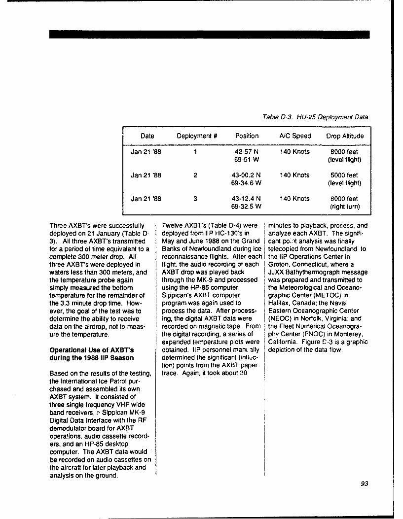
Table D-3. HU-25 Deployment Data.
Date Deployment # Position A/C Speed Drop Attitude
Jan 21 '88 1 42-57 N 140 Knots 8000 feet69-51 W (level flight)
Jan 21 '88 2 43-00.2 N 140 Knots 5000 feet69-34.6 W (level flight)
Jan 21 '88 3 43-12.4 N 140 Knots 8000 feet69-32.5 W (right turn)
Three AXBT's were successfully Twelve AXBT's (Table D-4) were i minutes to playback, process, anddeployed on 21 January (Table D- deployed from lIP HC-130's in analyze each AXBT. The signifi-3). All three AXBT's transmitted May and June 1988 on the Grand cant po'..t analysis was finallyfor a period of time equivalent to a Banks of Newfoundland during ice telecopied from Newfoundland tocomplete 300 meter drop. All reconnaissance flights. After each the liP Operations Center inthree AXBT's were deployed in flight, the audio recording of each Groton. Connecticut, where awaters less than 300 meters, and AXBT drop was played back JJXX Bathythermograph messagethe temperature probe again through the MK-9 and processed was prepared and transmitted tosimply measured the bottom using the HP-85 computer. the Meteorological and Oceano-temperature for the remainder of Sippican's AXBT computer graphic Center (METOC) inthe 3.3 minute drop time. How- program was again used to Halifax, Canada; the Navalever, the goal of the test was to process the data. After process- Eastern Oceanographic Centerdetermine the ability to receive ing, the digital AXBT data were (NEOC) in Norfolk, Virginia; anddata on the airdrop, not to meas- recorded on magnetic tape. From the Fleet Numerical Oceanogra-ure the temperature. the digital recording, a series of phv Center (FNOC) in Monterey,
expanded temperature plots were California. Figure C-3 is a graphicOperational Use of AXBT's obtained, lIP personnel manr ally depiction of the data flow.during the 1988 liP Season determined the significant (infi c-
tion) points from the AXBT paperBased on the results of the testing, trace. Again, it took about 30the International Ice Patrol pur-chased and assembled its ownAXBT system. It consisted ofthree single frequency VHF wideband receivers, n Sippican MK-9Digital Data Interface with the RFdemodulator board for AXBToperations, audio cassette record-ers, and an HP-85 desktopcomputer. The AXBT data wouldbe recorded on audio cassettes onthe aircraft for later playback andanalysis on the ground.
93

Table D-4. HC- 130H AXBT Deployments during 1988 liP Season.
Date Deployment # Position A/C Speed Altitude
May 3 1 46-15 N 150 knots 8000 feet46-05 W
May 3 2 46-15 N 150 knots 8000 feet46-35 W
May 3 3 46-15 N 150 knots 8000 feet47-00 W
May 18 1 43-00 N 150 knots 2000-2500 feet49-41 W (level flight)
May 18 2 43-00 N 150 knots 2000-2500 feet48-30 W (level flight)
May 18 3 43-00 N 150 knots 2000-2500 feet47-29 W (left turn)
Jun 4 1 42-15 N 150 knots 8000 feet47-00 W
Jun 4 2 42-15 N 150 knots 8000 feet47-40 W
Jun 4 3 42-15 N 150 knots 8000 feet48-20 W
Jun4 4 42-15 N 150 knots 8000 feet49-00 W
Jun 4 5 42-15 N 150 knots 8000 feet50-00 W
Jun 4 6 42-15 N 150 knots 8000 feet50-59 W
94

AXBT RF AudioCassetteSignal Recorder
VHF AXBTReceiver Audio
SignalAXBTAudioSignal MK-9
Audio Cassette 1 AXBTRecorder Digital
i Data
Ready for HP-85Next AXBT Computer
Deployment
Significant PointAnalysis and
JJXX Message j
AXBTTemperature
Profile
I Telecopier
[ iP OPCENGroton, CT
FNOC INMETOC
Figure D-3. AXBT Data Flow.
95

Typical temperature profiles from The six AXBT's deployed on 4 ° If local weather conditionsthe deployments are shown in June exhibited a wide variation in dictate dropping at other thanFigures D-4 through D-7. There is quality of performance, although optimum conditions, the followinga great variation in the quality of the deployment altitude and sea guidelines should be used inthe temperature profiles from the conditions were constant through- making a drop decision:twelve AXBT's. The profiles from out (Figures D-6 and D-7). All sixthe three AXBT's deployed on 3 temperature profiles were in a. As altitude decreasesMay 1988 were of the best quality general noisier than the tempera- or aircraft speed increases, the(Figure D-4). All three tempera- ture profiles of the AXBT's de- quality of the AXBT temperatureture profiles had some spikes in ployed on 3 May, which were also profile decreases, particularlythe profile, and the frequency of deployed from 8000 feet, although towards the end of the profile.spikes increased with depth (time). the sea conditions were muchThere were many white caps calmer on 4 June than on 3 May. b. A drop from 3000 feet,observed on the sea surnace when at 150 knots, P-1 -9 a steadythe AXBT's were deployed. Conclusions heading will bt; , ,eadable after
150 meters. If the aircraft turns orThe quality of the temperature - AXBT's are an excellent means circles around the drop site after aprofiles fro., the three AXBT's of gathering ocean temperature drop from 3000 feet, the tempera-deployed on 18 May 1983 was information at a relatively low cost ture profile will be readable to 200-very poor (Figure D-5). These to the U. S. Coast Guard and lIP. 250 meters, or the amount of dataAXBT's were deployed from a gathered is essentially doubled.relatively low altitude (2000-2500 * AXBT data can successfully befeet). The temperature profiles collected using a portable, low • The quality of the temperaturewere, overall, much noisier than cost, easy to operate, commer- profile decreases with increasingthe temperature profiles from 3 cially available system such as the sea state.May, despite the fact that the sea one presented here.conditions v - r much calmer on - The quality of the temperature18 May than 3 May. Static noise - lIP can conduct AXBT opera- profile decreases with time (depth)interference made the temperature tions from either the HC-1 30 or because the distance between theprofiles unreadable after 170-250 HU-25 without airframe modifica- aircraft and AXBT increases.meters. The temperature profile tions.which was readable down to 250 ° The loss of quality at lowmeters (deployment 3) was from • Optimum AXBT drop conditions i altitudes and at distance from thean AXBT deployed at the end of a are 4000-8000 feet and 150 knots. AXBT is due to poor transmissionsearch leg and shortly before a The aircraft should maintain 150 angle. A loss of line of sightturn. knots for the entire 3.3 minute occurs more frequently at low
drop time. transmission angles due to waveand swell action, particularly inhigh sea states. This causesinterference of the AXBT signaland spiking in the temperatureprofile.
96

Temperature (*C) Temperature (OC)
Figure D-4. HC- 130 Deployment 1 Figure D-5. HG- 130 Deployment 2May 3, 1988. May 18, 1988.
Temperature (OC) Temperature (OC)
±Ise
05.
Figure D-6. HC- 130 Deployment 1 Figure D- 7. HC- 130 Deployment 6June 4, 1988. June 4, 1988.
97

- Some of the interference or poor Future Plans - Since the AXBT information issignal reception may be due to useful to other U.S. and Canadianantenna location on the HC-1 30. For the 1989 International Ice users, pursuing cooperativeThe AXBT signal may be getting Patrol Season, liP plans the funding from these users. liPinterfered with too easily by having following: would provide the airframe with anthe antenna on the far right side of AXBT system, the user wouldthe aircraft fuselage. - Developing an AXBT system provide the AXBT's, and lIP and
which processes the data real- the users would share the data.* The data analysis method of time, and records the digital adatarecording the AXBT data on audio on computer floppy disk with ancassettes for later playback and audio taps recorder back-up.analysis might have worked fortesting of the AXBT system, but • Developing a program to recallwill not be adequate for routine the recorded AXBT data, display itAXBT operations. The present on the computer screen, andmethod is too cumbersome and it manually determine the significanttakes too long. There is a risk of points from the AXBT tracelosing data due to cassette displayed on the screen.recorder malfunction, as hap-pened during the first HU-25 test.Temperature changes or powerfluctuations can affect the reliabil-ity of the cassette recorder, whichin turn can affect the data.
• Recording the audio AXBT dataon audio cassettes also adverselyaffects the quality of the tempera-ture profile. Recording the audiosignal introduces high frequencynoise which results in the tem-perature trace being 0.5-10 Cwide. Recording the AXBT indigital form would eliminate thishigh frequency noise, and improvethe quality of the temperatureprofile.
98
iblilography
Bane, J.M., and M. H. Sessions, A Field Performance Test of theSIPPICAN Deep Aircraft-Deployed Expendable Bathythermograph, JL
ophL.Res., 89(C3), 3615-3621, 1984.
Boyd, J. D. , Improved Depth and Temperature Equations for SIPPICANAXBTs, J. Atmos. Ocean. Tech., 4(3), 545-551, 1987.
99

100

Appendix EInternational Ice Patrol's Side-Looking Airborne
Radar Experiment (SLAREX) 1988Lt M. A. Alfuttis, USCG
CDR S. R. Osmer, USCGAbstract 282). The HU-25 and HC- 130 unit of the U S. Coast Guard, has
aircraft flew a box pattern around provided this service since ftsDuring the period 7 through 16 the iceberg search area, Sever al initiation in 1914 From 1914 toJune 1988, the International Ice different attitudes were used 1945, UIP used visual roconnats-Patrol conducted an evaluation of sance f rom ships to monflor thethe ANIAPS-131 Side-Looking The Ice Branch of the Atmosphteric "cbergs. After World War 1I, anidAirborne Radar (SLAR). This Environment Service of Canada up to 1983, lIP used aircraft visualSLAR, installed as part of the also had two of its SLAR -equipped reconnaissance as its primarymufti-sensor su~rveillance AIREYE ice reconnaissance aircraft (an method of iceberg detiection.system onboard the U, S. Coast Electra and a Dash-7) participate Since 1983, lIP has utiltzed aGuard HU-258 medium endur- in the experiment. Motorola AN/APS-135 Side-ance aircraft, was evaluated for its Looking Airborne Radar (SLAP)ability to detect icebergs. The Results indicate the AN!APS-131, onboard HC-130H Hercules iong-data collection occurred in an while not having the azimuth range aircraft as its ponmaryiceberg infested area off the coast resolution of the AN/APS- 135, is method of iceberg reconinats-of Newfoundland, Canada. capable of performing the iceberg sance.
reconnaissance mission, TheseThe fundamental goal of this preliminary results indicate an In 1983, the U. S_ Coast Guardresearch was to provide guidance altitude of 4000 to 6000 feet is installed the Motorola AN/Al'S-on the ability of the AIREYE- best for the AN/APS-1 31 for this 131 SLAR as part of the airborneequipped HU-258 to perform the mission. multi-sensor surveillance AIREVEiceberg detection mission of the system on its HU-25B FalconInternational Ice Patrol. Specifi- Current plans for the 1989 iceberg medium- range aircraft. The AN/catty, there were two objectives: season are for the HU-258 to APS-131 SLAR is very similar to
icomplement the HC-130H recon- the AN/APS-135 SLAR on the HC-1. Determine the optimum Inaissance aircraft. Due to its 130, except that the antenna
altitude for iceberg reconnais- limited endurance, the HU-25B length of the Al'S-1 31 is half thatsance, and predict the probability aircraft will not be able to replace of the APS-1 35. This results inof detection as a function of sea the longer-range HC-130. How- the APS- 131 having a lowerstate, lateral range, and iceberg ever. during certain times of the azimuth resolution than the Al'S-size. iyear and in certain light ice years, 135. Although the iceberg detec-
the HU-25B should be able to fion ability of the Al'S- 135 SLAP2. Compare the iceberg I conduct the International Ice has been previously evaluated, no
detection capability of the AN/ iPatrol mission. evaluation of the iceberg detectionAPS-131 SLAR with the AN/AP.S- ability of the APS-1 31 SLAP has135 SLAR currently used on the jIntroduction been made.International Ice Patrol's HC-130long range reconnaissance After the sinking of the RMS The AIR EYE system on the HU-aircraft. TITANIC on April 14-15, 1912, an I258 contains other sensors in
International Ice Patrol Service addition to the SLAR, and are allGround truth (i.e. iceberg dimen- was created to monitor the pres- connected by a computerizedsions and positions, and environ- Ience of icebergs near the Grand multipurpose display system. Themental conditions) were collected Banks of Newfoundland, and to AIREYE system has a dry filmby the U. S. Coast Guard ice- warn mariners of these hazards. processor, as does the HC-130H.breaker NORTH WIND (WAGB The International Ice Patrol (lIP), a fThis film was the object of evalu-
ation.
101

This report presents the results of Aperture Radars (SAR) to detect both growlers and sma, icebergsan evaluation of the AN/APS-131 small icebergs and growlerm The in seas less than I m appear to beSLAR to detect icebergs. This M/V POLARIS provided surface just as detectable at lateral rangesevaluation was conducted by lIP truth data, Results of the data between 25 ano 50 km as they arefrom 7 to 16 June 1988 in the analysis reported in Rossiter et al at ranges less than 25 km Fi-North Atlantic Ocean off New- (1985) show greater detectability nally, they noted similar icebergfoundland, Canada. The funda- is obtained with lower sea states, detection performance of the ANvmental goal of this research was at lower attitudes within the APS-135 SLAR in this experimentto provide guidance on the ability operating envelope of each and in BERGSEARCH 84of the AIREYE-equipped HU-25B system, and when viewing targetsto perform the iceberg detection across rather than up or down Description of Aircraftmission of the International Ice wind and sea. BERGSEARCH 84Patrol. Specifically, there were data also demonstrated that ships A Coast Guard HC-130H and HU-two objectives: and iceberg targets generally do 25B were the two U S aircraft
not have different SLAR signa- used in the experiment The HC-1. Determine the best tures. 130H is a long-range tour engine
altitude for iceberg searches, and turboprop reconnaissance aircraft,predict the probability of iceberg The 1985 SLAR Detection Experi- whereas the HU-25B is a medium-detection as a function of sea ment was designed to determine range twin engine fan jet aircraftstate, lateral range, and iceberg SLAR's ability to detect various CG-1503 from Coast Guard Airsize. search and rescue and iceberg Station Elizabeth City. North
targets at all ranges out to 27 nm Carolina. was the HC-130H2. Compare the iceberg (50 km). The iceberg detection aircraft in the experiment, and CG-
detection capability of the APS- results reported in Robe et at 2103 from Coast Guard Air Station131 SLAR with the APS-135 (1985) indicate medium icebergs Cape Cod, Massachusetts, wasSLAR. are detectable nearly 100% of the the HU-25B. Table E-1 lists the
time in up to 2 m seas, small operating characteristics of theThis report will also compare the icebergs are easier to detect at two aircraft.results of this evaluation with the lower altitudes and with a smallerresults of two previous SLAR swath width, and growlers areiceberg detection evaluations, detectable more than 90% of the
time in seas less than 1 m. Also,Background
Previous SLAR Studies
Two previous SLAR studies have Table E- 1. Aircraft Operating Characteristics.
been conducted to evaluate the Aircraft HC-130H HU-25Bability of the AN/APS-135 SLAR todetect icebergs. During April Patrol Altitude 4-1O0000 ft 4.10.000 ft1984, BERGSEARCH '84 was Patrol Speed 180-250 kI 180-250 ktconducted to evaluate the ability of Endurance ,7.5 hr Q hrthree SLA~s and two Synthetic Navigation INS (LTN-72) AIRNAV (INS & LORAN)
Drop Capable Yes (Incl TOO) Yes (Incd mini-TOD)
102

Description of AN/APS- 135 and Table E-2. SLAR OperatiV Paraneters.AN/APS- 131 SLAR
Aicraft HC- 130H HU-258Significant system parameters ofeach SLAR are presented in Table SLAR (Reel A!enur. MotoroMoE-2. The major difference be- ANIAPS-• 35 ANjAPS. ¶31
tween the two systems Is the X.8" (9M MPz) X4Ua (925O MHz)antenna length of each. The APS- Peak Poww 200 ) d 200 K )135 has a 4.8 m long antenna,while the APS-131 "s antenna is Putle Wdth2.4 m long. This results in the Antennt CharacteristicsAPS-131 having one-half theazimuth resolution of the APS- Length 4.8 m 24 m135. Polarization VV VV
Elevation Coverage -1.5 to .45 dog A1 5 to -45 dogDescription of Targets Opa nAgD15dg1 e
Dopf'ossion Angle 1.5 dog 1.5dog
The USCGC NORTHWIND was Azimuth Resolution 0.47 deg 0.".g
the only surface vessel used as a Range Resolution 30 m 30 mSLAR target during the evaluation.The NORTHWIND is a U.S. Coast Receiver Bandwidth 8 MHzGuard wind-class icebreaker, and Swath Widths 25,50,100,150 km 25,50,100.150 km
is 81 m lon~g and 19 m wide. Look Direction L&FR L&R
Data Format Negative Film Negative FilmIIP classifies icebergs into five sizecategories: growler, small, VHS video I"p
medium, large, and very large.Table E-3 lists lIP's length andheight parameters for each sizecategory. A total of 44 icebergs Table E-3. lIPIwere used as targets during theevaluation, consisting of 13 small,27 medium, and 4 large icebergs. Descriptive Name Height Length
No growlers or very large icebergs (m) (mn)were used. Growler <5 <15
Small Iceberg 5-15 16-60
Medium Iceberg 16-45 61-122
Large Iceberg 46-75 23-213
Vey• Large Iceberg >75 >213
103

Table E-4. Range of Parameters.
Aircraft Target Lateral Search Significant Wind Speed Range ScalesRange Altitudes Wave (risec) (nm)(nm) (ft) Height (m)
Northwind 2-27 4,000 1-2,7 7 2-17 5 276,0008,00010,000
HC-130H(APS-135) Icebergs 2-27 4,000 1-2.7 72-17 5 27
6,0008,00010,000
Northwind 2-50 4,000 0.3-2.7 3 1-175 275,000 546,0008,000
HU-25B 10,000
(APS-131)Icebergs 2-50 4,000 0.3-2.7 3.1-17.5 27
5,000 546,0008,00010,000
Description of Environmental Data Collection Procedures responsible for selec rng the next
Conditions day's area of study around aGeneral group of iceberg targets, and
Seas were 1-2 meters during most passing the s!,;dy area coordi-
of the experiment. Table E-4 lists Data for this evaluation were nates to th' aircraft using VHF
the range of environmental and collected on 7-16 June 1988. The radio pri-r to the aircraft's depar-
operating parameters observed exact location of data collection ture- I ne next morning, the
and used during the experiment, varied with ice movement within a airc'aft would confirm the locationbox bounded by 510 N to 520 N ol NORTHWIND, and the study
and 52*30' W to 53'30' W (Figure area, after takeoff.E-1). Each evening, liP personnelon USCGC NORTHWIND were During the data collection runs,
the lIP crew on NORTHWINDmonitored the positions of eachiceberg in the study group, andrecorded surface environmentaldata.
104
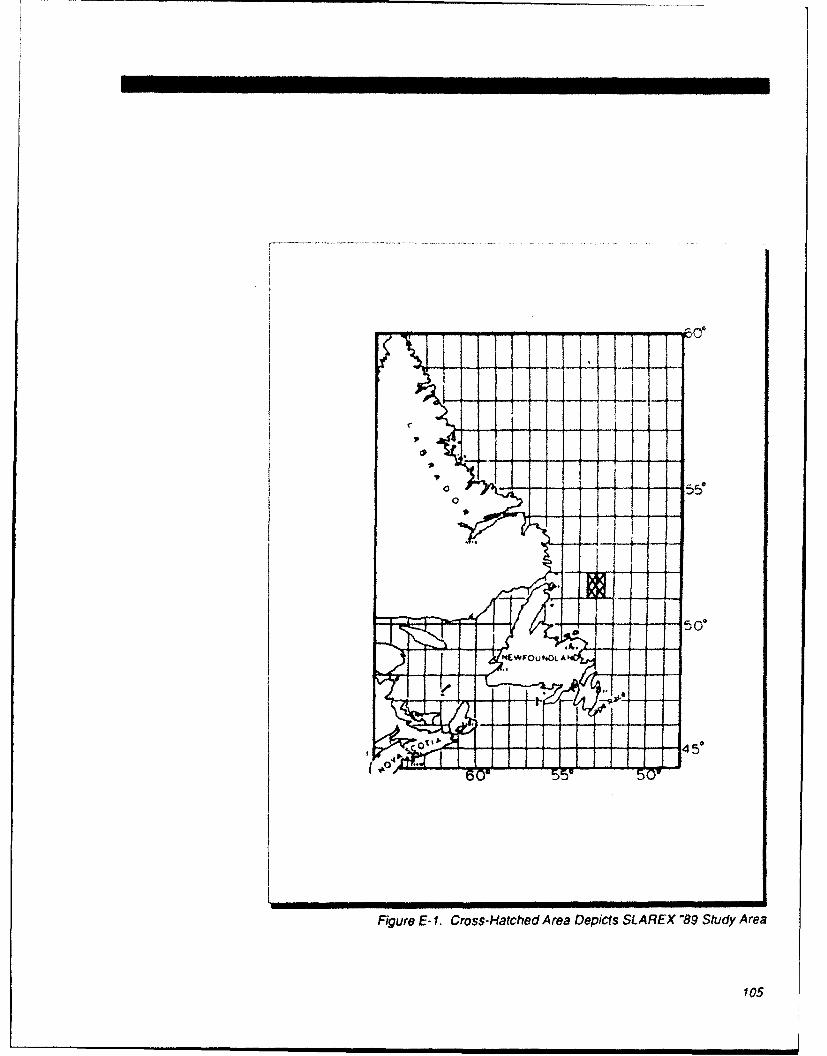
- - m - - -
I it
o -- ---- 550
N •EwFouNDo
T T
Figure E- 1. Cross-Hatched Area Depicts SLA REX "89 Study Area
105

s- 54 nm
%*csp
Figure E-2. TYPE I Search Pattern. CSP is Commerce Search Point.
Search Patterns Only the HU-25B flew the second used on this pattern. Because ofsearch pattern. ft was a parallel the limited amount of data col-
Two search patterns were used by line (type 2) search (Figure E-3). lected with the 54 nrm scale, no
the aircraft during the evaluation. This pattern was flown at 4000 discussion on the use of this scale
Most of the searches were an area and 8000 feet. The track spacing for ice reconnaissance will be
(type 1) search consisting of a was 6 nm (11 kim) for the first made in this report.
square with 54 nm (100 kin) sides three legs, and 12 nm (22 kim) for(Figure E-2). Both the HU-25B the last two legs. Both the 27 nmand HC-130H flew this pattern at (50 kin) and 54 nrm (100 km)four altitudes: 4000, 6000, 8000, range scale on the SLAR wereand 10,000 feet. All thesesearches were conducted usingthe 27 nm (50 kin) range ,.ale onthe SLAR.
106

T
25nm
S Scs is 27myw 27! !.~~cale •1
41 36 .24 15 12 6 0
RM"
Fagure E-3. Type 2 Search Pattern.
107

Table E-5 lists the pattern and Table E-5. Aircraft Search Pattern.altitude each aircraft flew for eachday of the experiment.
Date Aircraft Search Alt itude NumberSLAR Data Format Pattern (fM) of Sorties
The output analog imagery from 8 June HC-130 1 8000 2both the APS-131 and APS-135 HU-25 1 6000 1SLAR was recorded on 23 cmwide dry-process film. The HU- 9 June HC-130 1 4000 225B also used a video recorder to HC-130 1 6000 2record the analog imagery on VHS HC-130 1 10,000 2tape format. HU-25 1 6000 2
Two logs were maintained on the 10 June HU-25 1 8000 2aircraft to aid the data analysis. HU-25 1 4000 2The SLAR Search Run SummarySheets recorded the start and stop 11 June HU-25 1 10,000 2time of each leg; aircralt speed, HU-25 1 8000 2altitude, and heading; and SLARsettings. The second was a SLAR 12 June HU-25 1 4000 2Target Log to record latitude, HU-25 1 5000 2longitude, and time of each SLAR HC-130 1 4000 2target observed by the SLAR HC-1 30 1 6000 2operator, as well as the SLAR HC-130 1 8000 2operator's interpretation of the HC-130 1 10,000 2SLAR target (ship or iceberg, andiceberg size). The SLAR operator 13 June HU-25 2 8000 4also circled the target on the HU-25 2 4000 2SLAR film, and annotated the filmwith the target number from the 15 June HU-25 1 6000 2SLAR Target Log. HU-25 1 8000 1
HU-25 1 10,000 1
108

Table E-6. Total Detection Oppofluniries(Type I and Type 2 Searches. 27 and 54 nm Scales)
HU-25B HC-130H
(APS-131) (APS-135)
S 133 48
M 230 132
L 45 17
Northwind 76 31
Total 484 228
Surface Truth Data Post-Analysis
Every 15 minutes, UP personnel Following the experiment, liPon USCGC NORTHWIND re- personnel used the SLAR film,corded NORTHWIND's position SLAR Search Run Summaryand, bearing and range to every Sheets, SLAR Target Logs, andvisible ice target in the SLAR SLAR Target Position Records toTarget Position Record. Position reconstruct and describe eachdata were obtained from a GPS/ target detection opportunity. TheLORAN C receiver. The bearing lIP analysts correlated the SLARand range data were obtained Target Position Records with thefrom NORTHWIND's surface SLAR film to determine which ofsearch radar. Every 30 minutes, the documented targets werelIP personnel recorded surface discernible on the film.environmental conditions, includ-ing wind speed/direction, cloud Results and DIscussioncover, visibility, sea state, humid-ity, and air and water temperature. Table E-6 summarizes the total
number of detection opportunitiesfor each SLAR. Table E-7 showsthe distribution of the detectionopportunities with altitude andlateral range for each SLAR. Forthe APS-135, the detectionopportunities were distributedevenly between the four altitudes4,000, 6,000, 8,000, and 10,000feet and in the mid to far-range (5to 27 nm). For the APS-131, mostof the detection opportunities wereat 4,000 and 8,000 feet and in thefar range (15-27 nm).
109

Table E.7 Total Detection Opportunities as a Function of Alilitude and Lateral Range.
HC-130H (APS-135) Total Detection Opportunities(Type I Searches)
Range (nm)
0-4 5-9 10-14 15-19 20-27 Total
Altitude (ft)
4,000 1 15 14 7 18 55
5,000 0 0 0 0 0 06,000 0 14 12 14 20 60
81000 0 :,13 8 15 17 53
10,000 0 13 13 15 19 60
12,000 0 0 0 0 0
Total 1 55 47 51 74 228
HU-25B (APS-131) Total Detection Opportunities
(Type I and Type 2 Searches)
Range (nm)
0-4 5-9 10-14 15-19 20-27 27-50* Total
Altitude (1t)4,000 16 27 19 31 29 0 122
5.000. 0 9 2 11 11 0 336,000 2 16 10 17 17 0 62
8,000 8 37 38 52 28 202
10,000 3 1 5 10 22 0 41
12,000. 0 0 0 6 0 18 24Total 29 90 75 113 131 46 484
"27-50 nm ranges for Type 2 Searches only.
110

Table E-8. Probability of Detection as a Function of Iceberg Size(Type I and Type 2 Searches, 27 nm Scale)
Detections/Opportunities _,0D)
HU-258 HC- 130H
APS-131 APS-135
Small 1141116 (.98) 47/48 (,98)
Medium 200/203 (.96) 132/132 (1 00)
Large 36/36 (1.00) 17/17 (1.00)
Total 350/355 (.99) 196/197 (.99)
I Northwlnd /5I U(1.00) 31/31 (1,00)
Table E-8 lists the number of Table E-9 lists the Iceberg POD as Thes, results are similar to theSLAR detections over the number a function of lateral range and results obtained duringof detection opportunities, and the altitude. Again, both SLARs have BERGSEARCH '84 and the 1985probability of detection (POD), for a similar iceberg detection capabil- SLAR Detection Experiment, foreach SLAR as a function of ity at all altitudes and lateral the given type of targets and seaiceberg size (and for the NORTH- ranges. There is no significant conditions.WIND). The two SLARs have a variation in Iceberg POD withvery similar iceberg detection lateral range or altitude. There Iscapability. The iceberg POD (for a small decrease in iceberg PODsmall, medium, and large ice- at 8,000 and 10,000 feet for thebergs) for each SLAR is 99 APS-131 SLAR, however.percent.
111

Table E-9 Iceberg POD as a Function of Lateral Rang#e irl Altitude(Type I and 2 Searches. 27 nm Scale)
HC-130H HU-25B
Range (nm) APS-135 APS-1310-4 vi1 %I no') 24,24 (1t 00)
5-9 53153(100) 82/83(99)
10-14 42/42 (1 00) 62.163(98)
15-19 43/43 (1.00) &W ( 97)
20-27 57158 (,98) 97/97 (1 00)
HC-130H HU-258
Altitude (It) APS-135 APS-131
4,000 47/47 (1 00) 106,/105 (1 00)
5,000 929 (1 .00)
6.000 52/52 (1 00) 52/52 (1 00)
8,000 46/46 (1.00) 130/134 (97)
10,000 51/52 (.98) 31t32 (97)
12.000 3/3(1.00)
112

Table E- 10. Number of SLA? Targets Missed by SLAR Observers over Total Number cf SLAP Targets
HC-130H (APS-135) Operator Misses
Attitude (it)
4,000 5,000 6.000 8,000 10.000
S 0/12 0j12 1/12 1/11
M 2131 2316 7t29 2136
L 0/4 0/4 is5 014
Total 2/47 2152 9/46 3'51
Northwind 0/8 0/8 0/7 0/8
HU-258 (APS-131) Operator Misses
Attitude (It)
4,000 5.000 6.000 8.000 10,000
S 0/35 1/8 3/15 0/44 0/11
M 0/58 1/17 3.30 1174 0/20
L 0/12 0/4 0/7 0/12 0/0
Total 0/105 2/29 6/52 1/130 0/31
Northwind 0/17 014 1/110 0/27 019
Table E-1 0 shows the distribution Although there is not enough data observers, there is no clearof the number of SLAR targets to draw any clear conclusions, indication at which altitude themissed by the HC-130H and HU- some broad tendencies can be SLAR observers are most likely to25B SLAR observers over the total drawn from the data in Tables E- miss targets. The greatestnumber of targets detected by the 10 and E-11. For the HC-130H, percentage of misses was at 6000SLAR with altitude. Table E-11 there is an indication in Table E-10 feet, while the least percentage ofshows the distribution of HC-130H that the SLAR observer is more misses was at 8000 feet. Table E-and HU-25B SLAR operator likely to miss a target on the SLAR 11 indicates that the HC-130H andmisses with lateral range. film at attitudes 8000 feet and HU-258 SLAR observers are more
greater than at altitudes less than likely to miss targets at lateral8000 feet. For the HU-25B ranges greater than 15 nm than at
lateral ranges less than 15 nm.
113

Table E-1 1. Number of SLAR Targets Missed by SLAR Observers over Total Number of SLAR Targets,
HC-130H (APS-135) Operator Misses
Range (nm)
0-4 5-9 10-14 15-19 20-27
S 0/0 0/0 0/17 2/8 0122
M 0/1 3/37 0/24 3/35 7/35
L 0/0 1/16 0/1 0/0 0/0
Total 0/1 4/53 0/42 5/43 7/57
Northwind 0/0 0/2 0/5 0/8 0/16
HU-25B (APS-131) Operator Misses
Range (nm)
0-4 5-9 10-14 15-19 20-27
S 0/12 1/20 0/19 2/28 1/35
M 1/10 1/40 0/37 0/51 3/62
L 0/2 0/22 0/6 0/6 0/0
Total 1/24 2/82 0/62 2/85 4/97
Northwind 0/5 0/7 0/9 0/17 1/29
114

Table E- 12. HC- 130H Operator Object Misinterpretations.
Number of Incorrect Object Misinterpretationsvs Total Number of SLAR Targets
Attitude (ft)
4,000 6,000 8,000 10,000
S 0/12 0/12 0/12 2/11
M 1/31 0/36 1,29 2/36
L 0/4 0/4 0/5 0/4
Total 1/47 0/52 1/46 4/51
Northwind 1/8 0/8 3/7 6/8
Range (nm)
0-4 5-9 10-14 15-19 20-27
S 0/0 0/0 1/17 0/8 1/22
M 0/1 1/37 0/24 1/35 2/35
L 0/0 0/16 0/1 0/0 0/0
Total 0/1 1/53 1/42 1/43 3/57
SNorthwind 0/0 1/2 3/5 3/8 6/16
Table E-1 2 lists the distribution of Again, no clear conclusions can In addition to the data given inthe number of incorrect interpreta- be made from the data in Tables Tables E-10 through E-13, thetions by the HC-130H SLAR E-12 and E-13, but some tenden- quality of the SLAR imagery fromobservers over the total number of cies can be seen. Tables E-1 2 4000 and 6000 feet seemed betterSLAR targets with altitude and and E-13 indicate the HC-130H than from 8000 or 10,000 feet.lateral range. This table considers observers were more likely to The imagery of ships from 4000only whether the target was misinterpret the type and size of and 6000 feet was harder withwrongly interpreted as an iceberg the SLAR target at altitudes 8000 sharp edges, making it easier toor ship. Table E-13 lists the feet and higher, and at lateral differentiate between a ship or andistribution of HC-130H observer ranges greater than 10 nm. iceberg at these altitudes.misinterpretations of SLAR targetsize over total number of SLARtargets with altitude and lateralrange. Since the HU-25B SLARobservers were inexperienced atinterpreting SLAR data, they werenot considered.
115

Table E-13. HC-130H Operator Size Misinterpretations.
Number of Incorrect Size Interpretations vsTotal Number of SLAR Targets
Altitude (ft)
4,000 6,000 8,000 10,000
S 1/12 1/12 3/12 3/11
M 0/31 0/36 0/29 0/36
L 0/4 0/4 0/5 0/4
Total 1/47 1/52 3/46 3/51
Northwind 1/8 0/8 0/7 0/8
Range (nm)
0-4 5-9 10-14 15-19 20-27
S 0/0 0/0 3/17 2/8 3/22
M 0/1 0/37 0/24 0/35 0/35
L 0/0 0/16 0/1 0/0 0/0
Total 0/1 0/53 3/42 2/43 3/57
Northwind 0/0 1/2 0/5 0/8 0/16
116

Conclusions
For the given sea conditions andsize of targets, all altitudes andlateral ranges out to 27 nm appearsuitable for iceberg searches. Forthe APS-131 SLAR, an altitude of6,000 feet and lower appears tobe a slightly better altitude foriceberg reconnaissance than8,000 feet or higher. More studyis needed at higher sea states andwith smaller ice targets before anyfinal conclusions can be drawnregarding the optimum icebergsearch altitude and the POD as afunction of sea state, lateral range,and iceberg size.
The APS-131 is very similar in itsiceberg detection capability to theAPS-135. These results indicate itis capable of performing theiceberg reconnaissance mission ofthe International Ice Patrol.
Current plans for the 1989 icebergseason are for the HU-25B tocomplement the HC-130H recon-naissance aircraft. Due to itslimited endurance, the HU-25B
aircraft will not be able to replacethe longer-range HC-130H.However, during certain times ofthe year and in certain light iceyears, the HU-25B should be ableto conduct the International IcePatrol mission.
117

Bibliography
Rossiter, J.R., L.D. Arsenault, E.V. Guy, D.J. Lapp, and E. Wedler,"BergSearch '84: Assessment of Airborne Imaging Radars forthe Detection of Icebergs. Summary Report - Results, Conclu-sions, and Recommendations," Environmental Studies Revolv-ing Funds Project, CANPOLAR Consultants, Ltd, Toronto,Ontario, 1985.
Robe, R.Q., N.C. Edwards, Jr, D.L. Murphy, N.B. Thayer, G.L. Hover,and M.E. Kop, "Evaluation of Surface Craft and Ice TargetDetection Performance by the AN/APS-135 Side-LookingAirborne Radar (SLAR)", U.S. Coast Guard, Washington D.C.,1985.
U's. =OM •Wý T •'RINT VI Ic9Os OO-,A4/,OO6
118

570560 550 540530 520 51° 50"49" 48"'47' 46' 45 44 43 42: 41 40 39
520: 52
510- 51
50- *-50
4907 49
Newfoundland480 48
470 Grand Banks of FeihCp47
46 -0-46
4501 45
440 , 44
430-- •43
42°- 42
4!° 41
400° U40-
390-- denotes the mean position of the Labrador Current 39
3 8 0 ý r , , , ,' , , , , ,,, , , m,, , , , m m. , , , , , , , , , , , ,,, . . . . . . .. ..1. . . .1. ..1 M, . . . , • . . 3 8 ý '570 560 550 540 530 520 510 50" 490 480 470 460 45" 440 430 420 41 40" 39'z
Figure 33. This figure depicts the mean position of the Labrador Current,the main mechanism for transporting icebergs south to the Grand Banks.