Embed Size (px)
Citation preview
Nat.Lab. Report rep 7254
Date of issue: November 2002
Analysis of Quantization basedWatermarking
M. Staring
Company restrictedc©Philips Electronics Nederland BV 2003

rep 7254 Company restricted
Authors’ address data: M. Staring WY71;[email protected]
c©Philips Electronics Nederland BV 2003All rights are reserved. Reproduction in whole or in part is
prohibited without the written consent of the copyright owner.
ii c©Philips Electronics Nederland BV 2003

Company restricted rep 7254
Report: rep 7254
Title: Analysis of Quantization based Watermarking
Author(s): M. Staring
Part of project: VSP: 1996 - 355
Customer: Digital Networks
Keywords: Digital watermarking, quantization watermarks, QIM, DC-QIM, distor-tion compensation, SCS, adaptive quantization stepsize, error correctingcodes
Abstract: see pagev - vi
Conclusions: see page95 - 97
c©Philips Electronics Nederland BV 2003 iii
rep 7254 Company restricted
This is the graduation report of
M. Staring,
student Applied Mathematics at the University of Twente (UT), at the chair StochasticSystem and Signal Theory of the Systems, Signals and Control group.
This graduation project was carried out at Philips Research Laboratories in Eindhoven(Nat.Lab.) in the cluster Watermarking and Fingerprinting, from the group Processingand Architectures for Content Management (PACMan), from the sector Access and Inter-action Systems (AIS). The project was done from December 2001 till November 2002.
The graduation committee consists of the following people:
Prof. dr. A. Bagchi, UTProf. dr. P.H. Hartel, UTDr. Ir. J.C. Oostveen, Philips ResearchDr. J.W. Polderman, UT
Philips Research LaboratoriesProf. Holstlaan 45656 AA EindhovenThe Netherlands
University of TwenteDrienerlolaan 57522 NB EnschedeThe Netherlands
iv c©Philips Electronics Nederland BV 2003
Summary
In order to protect (copy)rights of digital content, means are sought to stop piracy. Several meth-ods are known to be instrumental for achieving this goal. This report considers one such method:digital watermarking, more specific quantization based watermarking methods. A general water-marking scheme consist of a watermark embedder, a channel representing some sort of processingon the watermarked signal, and a watermark detector. The problems related to any watermarkingmethod are the perceptual quality of the watermarked signal, and the possibility to retrieve theembedded information at the detector.
From current quantization based watermarking algorithms, like QIM, DC-QIM, SCS, etc., it isknown that the achievable rates are promising, but that it is hard to meet the required robustnessdemands. Therefore improvements of current algorithms are sought that are more robust againstnormal processing. This report focusses on two possible improvements, namely the use of errorcorrecting codes (ECC) and the use of adaptive quantization.
Watermarking can be seen as a form of communication. Therefore, the robustness demand forwatermarking is equivalent with the demand of reliable communication for communication mod-els. Therefore, the use of ECC gives certainly an improvement in robustness. This is confirmedby experiments. Repetition codes are simple to implement and already gives a gain in robustness.The concatenation of convolutional codes with repetition codes gives an improvement only in thecase of mild degradations due to the above mentioned processing.
In this report watermarking of signals with a luminance component are considered, like digitalimages and video data. Adaptive quantization refers to the use of a larger quantization step sizefor high luminance values, and a lower quantization step size for low luminance values. It isknown from Weber’s law that the human eye is less sensitive for brightness changes in higherluminance values, than it is in lower luminance values. Therefore, using adaptive quantizationdoes not come at the cost of a loss of perceptual quality of the host signal. Adaptive quantizationgives a large robustness gain for brightness scaling attacks. However, the adaptive quantizationstep size must be estimated at the detector, which potentially introduces an additional source oferrors in the retrieved message. By means of experiments it is shown that this is not such a bigproblem. Therefore, adaptive quantization improves the robustness of the watermarking scheme.
It is valuable to know the performance of the watermarking scheme with the two improvements.The used performance measure is the bit error probability. The total bit error probability is buildup from two components: One estimates the bit error probability for the case of fixed quantization,with an Additive White Gaussian Noise (AWGN) or uniform noise attack; The other estimates thebit error probability for the case of adaptive quantization, without any attack. Models for thesetwo bit error probabilities are developed.
At the embedder the distortion compensation parameterα has to be set. The optimal value for thisparameter is derived for the case of a Gaussian host signal and an AWGN channel. The value of
v

rep 7254 Company restricted
this optimal parameterα∗ is compared with an earlier result of Eggers [17] and is shown to beidentical. But whereas Eggers found a numerical function, which he numerically optimizes, ourresult leads to an analytical function, which can be optimized numerically.
So, we use two methods to improve robustness, namely the use of error correcting codes andan adaptive quantization step size. These two methods are shown to be improvements. Alsoan analytical model for the performance is derived, which can be used to verify analytically therobustness improvement.
vi c©Philips Electronics Nederland BV 2003
Acknowledgements
”Everything should be as simple as it is, but not simpler.”Albert Einstein (1879 - 1955)
First of all I would like to express my gratitude to Philips Research for the opportunity to workon an interesting and challenging subject like digital watermarking. I have enjoyed working atthe Nat.Lab., for it is a stimulating environment where people can grow to their highest potential.In writing this report, I have tried to keep things as simple as possible; Einstein’s quote is veryapplicable when writing a report!
I would like to express my gratitude to my supervisors, who helped me reach the project goals: JobOostveen and Ton Kalker from Philips Research and Jan Willem Polderman from the University ofTwente. Very valuable where the many discussions I had with them, other members of the groupand with fellow students; I really appreciated those discussions. Also, I would like to thank myparents, other family and friends for their support over the years.
Marius StaringEindhoven, November 2002
vii

rep 7254 Company restricted
viii c©Philips Electronics Nederland BV 2003

Contents
1 Preface 1
2 Introduction 3
2.1 What is digital watermarking?. . . . . . . . . . . . . . . . . . . . . . . . . . . 3
2.1.1 Information hiding. . . . . . . . . . . . . . . . . . . . . . . . . . . . . 3
2.1.2 Digital watermarking. . . . . . . . . . . . . . . . . . . . . . . . . . . . 4
2.1.3 Analogy with watermarks in banknotes. . . . . . . . . . . . . . . . . . 5
2.2 Applications. . . . . . . . . . . . . . . . . . . . . . . . . . . . . . . . . . . . . 6
2.3 Performance criteria and characteristics. . . . . . . . . . . . . . . . . . . . . . 7
2.3.1 Imperceptibility. . . . . . . . . . . . . . . . . . . . . . . . . . . . . . . 7
2.3.2 Robustness. . . . . . . . . . . . . . . . . . . . . . . . . . . . . . . . . 8
2.3.3 False positive and false negative probabilities. . . . . . . . . . . . . . . 9
2.3.4 Payload and Capacity. . . . . . . . . . . . . . . . . . . . . . . . . . . . 9
2.3.5 Security. . . . . . . . . . . . . . . . . . . . . . . . . . . . . . . . . . . 9
2.3.6 Computational cost. . . . . . . . . . . . . . . . . . . . . . . . . . . . . 9
2.3.7 Blind detection. . . . . . . . . . . . . . . . . . . . . . . . . . . . . . . 9
2.3.8 The trade-off between performance criteria. . . . . . . . . . . . . . . . 10
2.4 The Human Visual System. . . . . . . . . . . . . . . . . . . . . . . . . . . . . 10
2.4.1 Sensitivity . . . . . . . . . . . . . . . . . . . . . . . . . . . . . . . . . 10
2.4.2 Masking . . . . . . . . . . . . . . . . . . . . . . . . . . . . . . . . . . 13
2.4.3 Pooling . . . . . . . . . . . . . . . . . . . . . . . . . . . . . . . . . . . 13
2.5 Possible attacks on digital watermarks. . . . . . . . . . . . . . . . . . . . . . . 14
2.5.1 Arrangement of attacks. . . . . . . . . . . . . . . . . . . . . . . . . . . 14
2.5.2 Removal attacks. . . . . . . . . . . . . . . . . . . . . . . . . . . . . . 14
2.5.3 Synchronization attacks. . . . . . . . . . . . . . . . . . . . . . . . . . 17
2.5.4 Ambiguity attacks . . . . . . . . . . . . . . . . . . . . . . . . . . . . . 17
2.6 Different watermarking techniques. . . . . . . . . . . . . . . . . . . . . . . . . 17
2.6.1 Domain of embedding. . . . . . . . . . . . . . . . . . . . . . . . . . . 18
ix

rep 7254 Company restricted
2.6.2 Least Significant Bit (LSB) modification. . . . . . . . . . . . . . . . . 19
2.6.3 Spread Spectrum techniques. . . . . . . . . . . . . . . . . . . . . . . . 19
2.6.4 Patchwork Algorithm. . . . . . . . . . . . . . . . . . . . . . . . . . . . 20
3 Quantization Watermarking 23
3.1 The Ideal Costa Scheme. . . . . . . . . . . . . . . . . . . . . . . . . . . . . . 24
3.2 Quantization Index Modulation. . . . . . . . . . . . . . . . . . . . . . . . . . . 25
3.2.1 Quantization Index Modulation. . . . . . . . . . . . . . . . . . . . . . 25
3.2.2 Distortion Compensated Quantization Index Modulation. . . . . . . . . 26
3.3 Practical watermarking schemes. . . . . . . . . . . . . . . . . . . . . . . . . . 27
3.3.1 The Scalar Costa Scheme. . . . . . . . . . . . . . . . . . . . . . . . . . 28
3.3.2 Dither Modulation . . . . . . . . . . . . . . . . . . . . . . . . . . . . . 29
3.4 Embedding by binary dithered quantization with uniform quantization step size. 29
3.4.1 The basic scheme. . . . . . . . . . . . . . . . . . . . . . . . . . . . . . 29
3.4.2 Dithering . . . . . . . . . . . . . . . . . . . . . . . . . . . . . . . . . . 31
3.4.3 Distortion compensation. . . . . . . . . . . . . . . . . . . . . . . . . . 33
3.5 Spreading a message and repetition coding. . . . . . . . . . . . . . . . . . . . . 34
3.6 Scalar Costa Scheme detection. . . . . . . . . . . . . . . . . . . . . . . . . . . 36
3.6.1 Hard versus soft decision decoding. . . . . . . . . . . . . . . . . . . . 37
3.6.2 Detection by correlation. . . . . . . . . . . . . . . . . . . . . . . . . . 38
3.6.3 The threshold setting. . . . . . . . . . . . . . . . . . . . . . . . . . . . 39
3.7 Summary . . . . . . . . . . . . . . . . . . . . . . . . . . . . . . . . . . . . . . 41
4 Problem description and Contributions 43
5 Enhancing robustness using Error Correcting Codes 45
5.1 The gain from using Error Correcting Codes. . . . . . . . . . . . . . . . . . . . 45
5.2 Convolutional Codes. . . . . . . . . . . . . . . . . . . . . . . . . . . . . . . . 46
5.2.1 Shift-register approach. . . . . . . . . . . . . . . . . . . . . . . . . . . 47
5.2.2 Convolutional representation. . . . . . . . . . . . . . . . . . . . . . . . 47
5.2.3 State representation. . . . . . . . . . . . . . . . . . . . . . . . . . . . . 49
5.3 Viterbi decoder . . . . . . . . . . . . . . . . . . . . . . . . . . . . . . . . . . . 50
5.4 Experimental results for ECC in the SCS. . . . . . . . . . . . . . . . . . . . . . 51
5.4.1 Experiment description. . . . . . . . . . . . . . . . . . . . . . . . . . . 51
5.4.2 Results and discussion. . . . . . . . . . . . . . . . . . . . . . . . . . . 53
6 Enhancing robustness using an adaptive quantization step size 59
x c©Philips Electronics Nederland BV 2003

Company restricted rep 7254
6.1 Advantages and disadvantages. . . . . . . . . . . . . . . . . . . . . . . . . . . 59
6.1.1 Advantages. . . . . . . . . . . . . . . . . . . . . . . . . . . . . . . . . 59
6.1.2 Disadvantages. . . . . . . . . . . . . . . . . . . . . . . . . . . . . . . 60
6.2 The adaptation rule. . . . . . . . . . . . . . . . . . . . . . . . . . . . . . . . . 60
6.3 Experimental results for an adaptive quantization step size. . . . . . . . . . . . 63
6.3.1 Experiment description. . . . . . . . . . . . . . . . . . . . . . . . . . . 63
6.3.2 Results and discussion. . . . . . . . . . . . . . . . . . . . . . . . . . . 63
7 Performance analysis 69
7.1 A measure for the performance. . . . . . . . . . . . . . . . . . . . . . . . . . . 69
7.2 The bit error probability due to a noise attack. . . . . . . . . . . . . . . . . . . 70
7.2.1 The derivation of the bit error probability. . . . . . . . . . . . . . . . . 71
7.2.2 The bit error probability for Gaussian noise. . . . . . . . . . . . . . . . 73
7.2.3 The bit error probability for uniform noise. . . . . . . . . . . . . . . . . 76
7.3 The bit error probability due to the adaptive quantization step size. . . . . . . . 80
7.3.1 Modelling the bit error probabilityP∆ . . . . . . . . . . . . . . . . . . . 80
7.3.2 Fourier approximation. . . . . . . . . . . . . . . . . . . . . . . . . . . 82
7.3.3 Convergence analysis. . . . . . . . . . . . . . . . . . . . . . . . . . . . 84
7.3.4 Statistics . . . . . . . . . . . . . . . . . . . . . . . . . . . . . . . . . . 85
7.4 Summary . . . . . . . . . . . . . . . . . . . . . . . . . . . . . . . . . . . . . . 87
8 Parameter optimization 89
8.1 The optimization problem forα . . . . . . . . . . . . . . . . . . . . . . . . . . 89
8.2 Bit error minimization and Eggers. . . . . . . . . . . . . . . . . . . . . . . . . 92
9 Contributions, Conclusions and Recommendations 95
9.1 Contributions . . . . . . . . . . . . . . . . . . . . . . . . . . . . . . . . . . . . 95
9.2 Conclusions. . . . . . . . . . . . . . . . . . . . . . . . . . . . . . . . . . . . . 96
9.3 Recommendations. . . . . . . . . . . . . . . . . . . . . . . . . . . . . . . . . . 96
A Notation 99
B Images 101
C Graphs for P∆ 103
References 107
Index 111
c©Philips Electronics Nederland BV 2003 xi

rep 7254 Company restricted
xii c©Philips Electronics Nederland BV 2003
Chapter 1
Preface
In today’s modern world, digital products are seen everywhere. The digitalization of all kinds ofmedia, like digital audio and video, has a lot of benefits for the consumer. Copying and distributingdigital content has become relatively simple with the introduction of computers and (fast) internet.But there are also some drawbacks. Analog video, for example, has a build in copy protectionsystem. An analog copy results in quality degradation, and a copy of a copy of an analog videohas degraded so much, that it is not a pleasure to look at. Digital video however doesn’t havethis build in copy protection system, because a copy of a digital video is identical to the original;There is no quality loss. Therefore it has become difficult for people to protect their intellectualproperties, like the intellectual rights on a digital video.
Methods to prevent the illegal copying of digital video has been sought since. One way of pre-venting illegal copying is the use of digital watermarks. This is the subject of the report.
Watermarking for example digital video is changing the video sequence slightly, in such a waythat at a later time, this slight change can be detected. For example, if a DVD recorder is equippedwith such a detection device, it can search for a watermark in all video offered for copying. Ifa watermark is found, copying is denied. In this way digital watermarking can provide a copyprotection mechanism.
Two of the most important demands that have to be met for watermarking digital content are thefollowing. The slight change made to the content, has to be slight indeed; People should not beable to see or hear (in the case of audio) that an image, a video sequence, an audio stream, etc., iswatermarked. The second demand is that the watermark should not get lost very easily. For exam-ple: modern televisions are utilized with image format buttons in order to switch between screenratio’s of 4:3 and 16:9. The watermark should still be detectable after such a switch. Other thingsa watermark should be able to resist are, for example, the broadcasting of video over satellites,conversions from one format to another (for examplewav to mp3 for audio), etc.
This report focusses on improvements of an existing watermarking algorithm in order to get betterresults for the above mentioned two demands. In Chapter2 and3 a general introduction to digi-tal watermarking and to a specific existing watermark algorithm are given, respectively. Only inChapter4 a more detailed problem description is given, because at that point the necessary termi-nology has been derived. In later chapters, possible solutions to the problems stated in Chapter4are derived.
In this report some abbreviations are used which the reader might not be familiar with. Theseabbreviations, together with the notation used in this report, are listed in AppendixA and the
1

rep 7254 Company restricted
Index, see page99.
2 c©Philips Electronics Nederland BV 2003
Chapter 2
Introduction
In this chapter digital watermarking is defined (see Section2.1) and some of its applications aregiven in Section2.2. In Section2.3 criteria are given to judge the quality of a watermarkingprocess. Some characteristics of the Human Visual System (HVS) are given in Section2.4and inSection2.5 some of the possible attacks on digital watermarks are described. Finally, in Section2.6, possible methods to put a watermark in digital content are considered.
For the general principles of digital watermarking the reader is referred to the excellent book ofCox, Miller and Bloom, see [14].
2.1 What is digital watermarking?
In order to understand what digital watermarking is, it is good to understand the principle ofhiding information, because digital watermarking can be seen as a part of Information Hiding.In Subsection2.1.1 Information Hiding is treated. The general principles of watermarking arediscussed in Subsection2.1.2. In Subsection2.1.3an analogy with banknotes is drawn.
2.1.1 Information hiding
Information Hiding is the process of sending information from one party to another, such thateither the message or the identity of the sender and the receiver is ’hidden’. Hidden means that themessage can not be read or removed by a third party, either because they don’t know the existenceof the hidden message or they are not capable of doing this.
Already in the early days of history, in the time of the ancient Greek, people used informationhiding techniques. One example (see [27]) tells about Histiaeus who informed his allies about theexact moment to revolt against the Persians, by shaving the head of a trusted slave and tattooing amessage on his head. The hair of the slave grew back on and the slave was send through enemyterritory, looking like an innocent traveller. On his arrival, the slave just told the allied leader toshave his head an read the message hidden there.
According to [27] Information Hiding can be divided into four categories:
Covert channels: Covert channels are communication channels that can be exploited by a pro-cess to transfer information in a manner that violates the systems security policy. So, for
3

rep 7254 Company restricted
example, information is carried over unintentionally by a computer program, to a user of thesystem.
Steganography: Steganography comes from the Greek wordssteganosand graphie, meaning”covered” and ”writing”. It comprehends the hiding of a secret message into a host message,such that nobody suspects its existence.
Anonymity: Anonymity is the communication of a message in which not the message itself isthe secret, but the sender or the receiver or both.
Watermarking: Watermarking is steganography plus a robustness (see Section2.3) requirement;Watermarking refers to the hiding of a message in a host message in such a way that if thissignal is altered, the hidden message still survives if the host survives.
So watermarking can be seen as a form of hiding information. Steganography and watermarkingare somewhat alike, because both methods have the goal to hide a message in a host signal. Thereare however three differences between watermarking and steganography:
1. Watermarking considers information about the object, the host signal, where for steganog-raphy the hidden message can be anything.
2. The robustness criteria are different. Steganography has the objective that information mustremain hidden, where watermarking has the objective that the information must not be re-moved, altered or damaged, even if the watermarking algorithm is known to the adversary.
3. Usually steganography is one-to-one and watermarking one-to-many; For steganographythere is usually one sender and one receiver, and for watermarking there is usually onesender and many receivers.
2.1.2 Digital watermarking
Digital watermarkingis the watermarking of digital content, like digital images, digital audio ordigital video. This digital content is often referred to as thehost signalor thehost data.
Digital watermarking is the process of making small adjustments to the host signal, in such away that these adjustments cannot be perceived by humans. These small changes represent insome way the information one wishes to hide. The changes are called thewatermark. The hostsignal together with the watermark adjustments is called thewatermarked signal. If the hostsignal is represented byx and the watermarked signal byy, then the watermark, represented byw, is defined asw � y − x, i.e., the difference between the watermarked and the host signal.Unless stated otherwise the signal are supposed to beN -dimensional vectors in the real space. Sox = (x1, · · · , xN ), y = (y1, · · · , yN ), with xi, yi ∈ R, i ∈ {1, 2, · · · , N}.
The process of watermarking a host signal is usually referred to asembeddinga message in the hostsignal. The process of reading the message at the receiver side is usually referred to asdetectinga message from the received signal. The devices that embed or detect a watermark are called theembedderand thedetector, respectively.
Watermarking can be seen as a form of communication. A general communication model is de-picted in2.1. After a messagem is embedded into a host signalx, the watermarked signaly issent over some channel to the receiver. On the path from the sender to the receiver processing
4 c©Philips Electronics Nederland BV 2003
Company restricted rep 7254
mEmbedderm w
x
y = x + w
n
r Detector
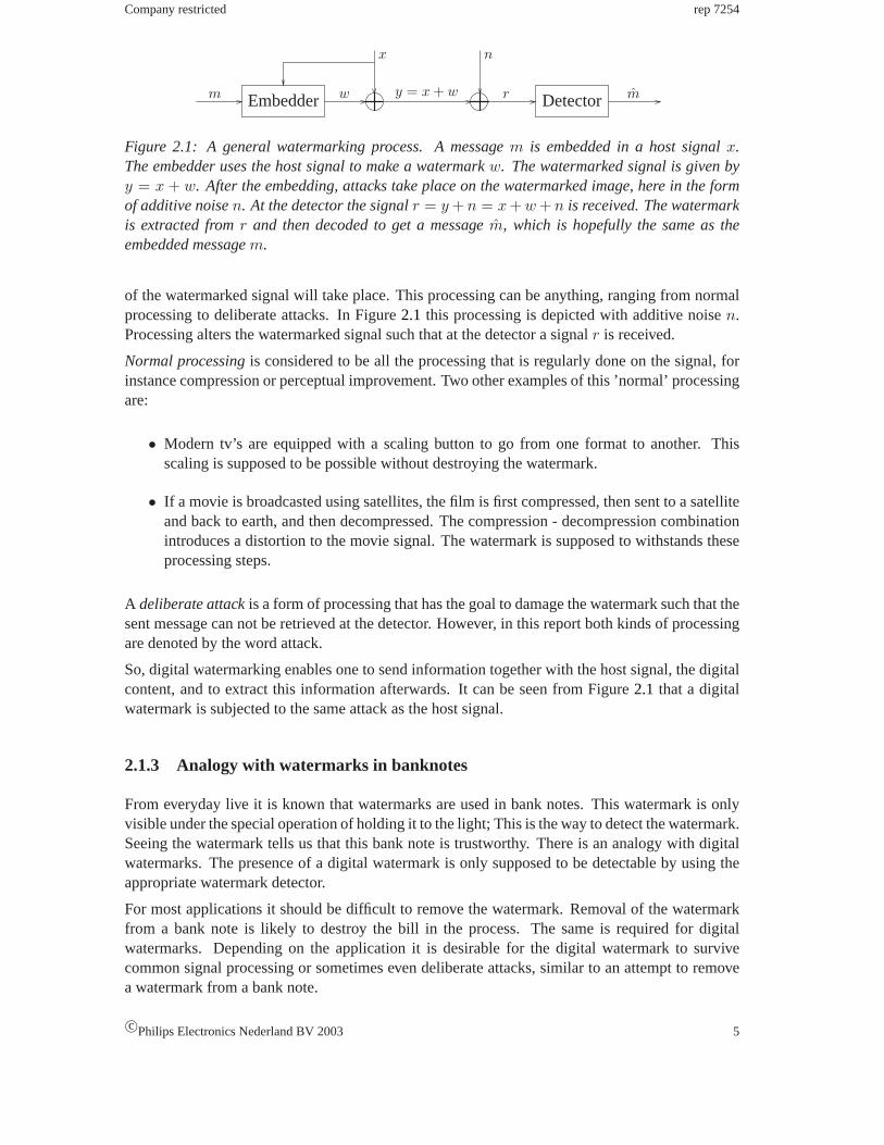
Figure 2.1: A general watermarking process. A messagem is embedded in a host signalx.The embedder uses the host signal to make a watermarkw. The watermarked signal is given byy = x + w. After the embedding, attacks take place onthe watermarked image, here in the formof additive noisen. At the detector the signalr = y + n = x + w + n is received. The watermarkis extracted fromr and then decoded to get a messagem, which is hopefully the same as theembedded messagem.
of the watermarked signal will take place. This processing can be anything, ranging from normalprocessing to deliberate attacks. In Figure2.1 this processing is depicted with additive noisen.Processing alters the watermarked signal such that at the detector a signalr is received.
Normal processingis considered to be all the processing that is regularly done on the signal, forinstance compression or perceptual improvement. Two other examples of this ’normal’ processingare:
• Modern tv’s are equipped with a scaling button to go from one format to another. Thisscaling is supposed to be possible without destroying the watermark.
• If a movie is broadcasted using satellites, the film is first compressed, then sent to a satelliteand back to earth, and then decompressed. The compression - decompression combinationintroduces a distortion to the movie signal. The watermark is supposed to withstands theseprocessing steps.
A deliberate attackis a form of processing that has the goal to damage the watermark such that thesent message can not be retrieved at the detector. However, in this report both kinds of processingare denoted by the word attack.
So, digital watermarking enables one to send information together with the host signal, the digitalcontent, and to extract this information afterwards. It can be seen from Figure2.1 that a digitalwatermark is subjected to the same attack as the host signal.
2.1.3 Analogy with watermarks in banknotes
From everyday live it is known that watermarks are used in bank notes. This watermark is onlyvisible under the special operation of holding it to the light; This is the way to detect the watermark.Seeing the watermark tells us that this bank note is trustworthy. There is an analogy with digitalwatermarks. The presence of a digital watermark is only supposed to be detectable by using theappropriate watermark detector.
For most applications it should be difficult to remove the watermark. Removal of the watermarkfrom a bank note is likely to destroy the bill in the process. The same is required for digitalwatermarks. Depending on the application it is desirable for the digital watermark to survivecommon signal processing or sometimes even deliberate attacks, similar to an attempt to removea watermark from a bank note.
c©Philips Electronics Nederland BV 2003 5

rep 7254 Company restricted
For a bank note it should not be possible to recreate the watermark and in doing so being ableto create trustworthy bank notes. This is also required for digital watermarks. It should not bepossible for unauthorized persons to detect, extract or insert a digital watermark from or in audio-visual content. These aspects are referred to as thesecurityof a digital watermark.
These, and more, requirements for digital watermarks are discussed in more detail in Section2.3.
2.2 Applications
Digital watermarking can be used for a variety of applications. In [13, 22, 27] a number of themare given:
Proof of ownership: It is possible to embed a watermark in digital content representing copyrightinformation. In this case the information might prove who is the copyright owner of thedigital content. It should be a hard task to remove the watermark.
Fingerprinting: It is possible to embed a watermark representing a customer identifier. If anillegal copy of the digital content is found, the copyright owner is able to trace it back to thecustomer by reading the watermark on the illegal copy.
Copy Protection: It is possible to embed a watermark in audio-visual content representing a copystatus (e.g. copy once, free to copy, copy never). A watermark detector reads this copy statusmessage and depending on the nature of this message the digital recorder can decide whetheror not to copy the content.
Broadcast Monitoring: In any broadcasted media, like commercials or television programs, it ispossible to embed a watermark. A watermark detector can automatically check if this mediaitem was actually broadcasted. ”Other applications include verification of commercial trans-missions, assessment of sponsorship effectiveness, protection against illegal transmission,statistical data collection, and analysis of broadcast content [27].”
Data Authentication or Tamper Proofing: It is possible to use a fragile watermark, see Subsec-tion 2.3.2, to determine if digital content is altered, by checking whether or not the water-mark is altered. In this case the watermark should be robust against small modifications, butnot against larger modifications. An example is the removal or insertion of a person into animage of a crime scene: the watermark should not be robust against this kind of modifica-tions, where it should be robust against minor modifications like lossy compression.
Indexing or Feature Tagging: The watermark can also represent additional information aboutthe content, like comments, captions or information useful for search engines (keywords).The security requirements are not relevant in this case, because indexing is considered aservice, so it is unlikely that someone wants to remove the watermark.
Medical safety: In order to not accidently combine an x-ray image with the wrong patient, it ispossible to embed a patients name on the x-ray image. In this case high demands have to bemet with respect to the imperceptibility of the watermark, because a doctor does not wantany uncertainty whether something on his x-ray image is a tumor or just some watermarkartefact.
6 c©Philips Electronics Nederland BV 2003

Company restricted rep 7254
Data hiding: A non-perceptible message embedded in digital content can contain secret or justhidden information. It is for example possible for terrorists to communicate secretly usingdigital images on an internet-site.
The first two applications together are usually referred to ascopyright protection.
2.3 Performance criteria and characteristics
In order to judge the quality of a watermark embedding algorithm, some criteria are given. Thereare several criteria, some of them already mentioned. Depending on the application some proper-ties are more important than others. For example for medical safety applications (see Section2.2)it is important that the watermark is absolutely imperceptible, but not necessarily robust againstsignal processing. For copy protection the imperceptibility properties are still high, but not thatabsolute. The robustness demands are very high in this case.
The following characteristics of watermarking algorithms are considered: imperceptibility, robustand fragile watermarks, false positive and false negative probabilities, payload and capacity, secu-rity, computational cost, blind and non-blind detection. These criteria are described in Subsection2.3.1- 2.3.7. In Subsection2.3.8the relations between those criteria are given.
2.3.1 Imperceptibility
A first criterion is that of the already mentionedimperceptibilityof the watermark. A watermark istruly imperceptible if humans cannot distinguish the original from the watermarked data if they arelaid side by side. Sometimes this is relaxed to the condition that one cannot see the watermark ifthe original data is not available for comparison. Imperceptibility is also referred to asperceptualtransparency.
In practical situations it is sometimes necessary to allow some amount of perceptibility of thewatermark. But how to measure this amount? The best way would be to use the human sensesto determine the perceptibility, because this is the ultimate criterion for deciding whether or not awatermark is perceptible for humans. Unfortunately, this is not convenient for practical purposes.Therefore, some sort of objective measure of perceptibility is used. The best objective measuresare those that imitate the human senses. Unfortunately, these measures are really complex, becausethe models of the Human Auditory System (HAS), for audio, or the Human Visual System (HVS),for still images or video, are complex. Therefore three rather simple measures to establish theperceptibility of a watermark are used: the Signal-to-Noise Ratio (SNR, the watermark is seen asnoise), theMean Squared Error(MSE) and for still images the Watson-metric. Because this reportis focused on still images, a description of the HVS is given in Section2.4.
The idea behind the use of theSignal-to-Noise Ratiois that a watermark is less perceptible if itsenergy is low compared to that of the host signal. The SNR is defined as:
SNR � 10 log10
(σ2
x
σ2w
), (2.1)
c©Philips Electronics Nederland BV 2003 7

rep 7254 Company restricted
wherex is the host signal (the digital content),w the watermark andσ2 the variance, whichrepresents the energy. The variance ofx, σ2
x, is calculated as usual as:
σ2x =
1N − 1
N∑i=1
(xi − x)2, (2.2)
wherex is the mean value ofx. σ2w is calculated in the same way. Another distortion measure is
the MSE, which is defined as
MSE � 1N
N∑i=1
(yi − xi)2 =1N
N∑i=1
w2i . (2.3)
The SNR and the MSE are more a measure of distance than of perceptual distance.
The Watson-metric is more like a measure of the perceptual distance. This distance is calculatedusing the Watson model which takes into account three factors: contrast sensitivity, luminancemasking and contrast masking. This metric is a little more sophisticated than just using the SNR,because it takes into account some aspects of the Human Visual System, see Section2.4. For adescription of the Watson model see Section 2.3 of [26].
Sometimes also visible (but not disturbing) watermarks are used, but we will not consider thosekind of watermarks. We will focus on imperceptible watermarks.
2.3.2 Robustness
Another important criterion already mentioned is that of therobustnessof a certain watermarkingalgorithm. According to [9], a truly robust watermark is a watermark that survives signal process-ing whenever the host signal does. In other words, robustness is the ability to withstand normalprocessing of the watermarked signal.
Two criteria for robustness are used in this study, robustness against noise and against lossy com-pression. Robustness against noise is measured as follows. White Gaussian noise is added to thewatermarked image and it is checked if it is still possible to detect the embedded information. Themaximum amount of noise added, after which it is still possible to detect the information, can beconsidered as a measure for robustness against noise. Also the bit error rate at certain values ofnoise power can be considered as robustness measure. In order to check robustness against lossycompression techniques, JPEG compression on the watermarked image is performed. The mini-mum JPEG quality factor used, after which it is still possible to correctly detect the watermark, isconsidered as a measure for robustness against lossy compression.
It is possible to determine the probability that after a noise attack a detected message bit is differentfrom the embedded message bit. This bit error probability as a function of the noise energy canalso be seen as a measure for robustness against noise.
There are also other types of digital watermarks, like fragile ones. Afragile watermarkis theopposite of a robust one. If the host data is somehow altered, this should be visible in the detectionresult. Sometimes it is important to prove that a photograph of e.g. a crime scene is not altered.This could be proved in court by showing that the fragile watermark has not been changed.
Because in most applications the watermark should be robust, we do not consider fragile water-marks, but robust ones.
8 c©Philips Electronics Nederland BV 2003

Company restricted rep 7254
2.3.3 False positive and false negative probabilities
A false positiveis a detection of a watermark while no watermark is embedded. Thefalse positiveprobability is the probability that a false positive occurs. Afalse negativeis no detection whilea watermark is embedded. Thefalse negative probabilityis the probability of such a missed de-tection. The relevance of these probabilities depends on the application. For the case of DVDvideo copy protection it should never happen that a DVD recorder refuses to copy something theuser has made himself (and is therefore not watermarked, at least not with the correct watermark).Therefore the false positive probability should be very low in this case. The false negative proba-bility is in this case not as important as the false positive probability; It is not a really big problemif a user makes an illegal copy every now and then, as long as this is within limits. In general thefalse negative probability is important for most applications, because this probability representsthe robustness of a watermark.
2.3.4 Payload and Capacity
The payloadis the amount of information that can be embedded in the host data. Thecapacityis defined as the amount of information that can be embedded and detected without errors. Theseamounts depend on the host data and on the watermarking algorithm. Directly related to capacityis therate. The rate is defined as the capacity divided by the total lengthN of the host signal.
2.3.5 Security
The securityof a watermark relates to the (in)ability to detect, remove or insert a watermarkfrom or in the host signal. UsingKerckhoffs’ principle[21], a watermark should still be secureif the watermarking algorithm is known to the adversary. Security must lie in the use of a secretkey. Security is the ability to withstand active (deliberate) attempts to disable the communicationthrough the watermark channel. Security also relates to the total watermarking system. If it ispossible for example to bypass the hardware in a DVD recorder that detects the watermark in aDVD, then the system is not secure, although the watermarked secret has not been compromised.
2.3.6 Computational cost
Thecomputational costis the effort it takes to embed or detect a watermark. This can be measuredin time, like clock cycles of a computer, but also in the need of extra memory capacity (thusmaking an application more expensive). The importance of this criterion varies per application.For example for broadcast monitoring the detection must be done in real-time, so the speed isimportant, but for copyright protection the speed is not important.
2.3.7 Blind detection
At the detector the original data may or may not be available for comparison with the received data.The absence of the original data at the detector is referred to asblind detection. It is clear that withnon-blind detection it is easier to check for a watermark. In practice, however, the original data isusually not known at the detector. We will therefore focus on blind detection.
c©Philips Electronics Nederland BV 2003 9

rep 7254 Company restricted
PerceptualTransparency
RobustnessPayload
Figure 2.2: Mutual dependencies between the performance criteria. Partially reproduced from[22].
2.3.8 The trade-off between performance criteria
In order to make a watermark very robust, very large modifications to the host data are needed.But, in doing so the watermark is made perceptible. This is an important observation, because itis telling us that for an optimal watermark a trade-off has to be made between the performancecriteria. A large payload will come at the cost of reduced robustness and perceptual transparency.The relationships between the criteria are shown in Figure2.2.
2.4 The Human Visual System
In order to measure the impact of a watermark in terms of perceptibility, some knowledge oftheHuman Visual System(HVS) is needed. Another reason to consider the HVS is that it givesinformation about the regions in which the human eye is insensitive. Those regions are a perfectoption to embed the information in, because larger modifications are possible, without the humaneye detecting them. In this section some basic characteristics of the HVS are treated. See [10, 14,29, 30] for more on this subject.
The sensitivity of the human eye for certain stimuli is treated in Subsection2.4.1. The fact thatcertain stimuli can be masked with others is considered in Subsection2.4.2. Pooling is treated inSubsection2.4.3.
2.4.1 Sensitivity
The two most important sensitivity characteristics for the human eye are brightness and frequencysensitivity. Brightness sensitivityrefers to the fact that the human eye is less sensitive to brightersignals, i.e., it will take a larger difference in bright signals than in signals with low luminancein order for humans to perceive it. Therefore it is possible to embed more of the watermark inregions with higher brightness. This principle is depicted in Figure2.3.
A just noticeable difference is the amount two stimuli need to differ by in order for the differenceto be perceived.Weber’s lawstates that these just noticeable differences are a function of thepercentage change in stimulus intensity not the absolute change in stimulus intensity. This meansfor example that the perceived difference between the light intensity of 10 and 11 candles in aroom is not the same as the perceived difference of 100 and 101 candles, but rather the differenceof 100 and 110 candles. So the bigger the stimulus the bigger a change required for it to seem
10 c©Philips Electronics Nederland BV 2003

Company restricted rep 7254
100
10
10 10 20 30 40 50 60 70 80 90 100
Luminance of uniform background (%)
Varia
nce
ofju
stno
tvis
ible
nois
e
Figure 2.3: Reproduced from [29]. The effect of background luminance on the maximum contrastof a just-not-visible noise pattern. Zero luminance corresponds to a black background on a CRTdisplay; a luminance level of 100 % corresponds to a white background on a CRT display. Atluminance levels around 30 % the human eye is most sensitive to noise patterns. The straightdashed line through the origin represents Weber’s law.
different. In order to perceive light differences the percentage two stimuli should differ is around6 %. A mass difference can be detected by humans if it is more than 2 % and a sound frequencydifference if it is more than 0.3 %. So the human ear is much more sensitive than the human eye,therefore it is more difficult to embed information in audio than in video. As can be seen fromFigure2.3, Weber’s law holds for luminance levels over 30 %.
Frequency sensitivitycan be divided into three forms for vision: spatial, spectral and temporal fre-quency sensitivities. Spatial frequencies are perceived as patterns or textures, spectral frequenciesas colors and temporal frequencies as motion or flicker.
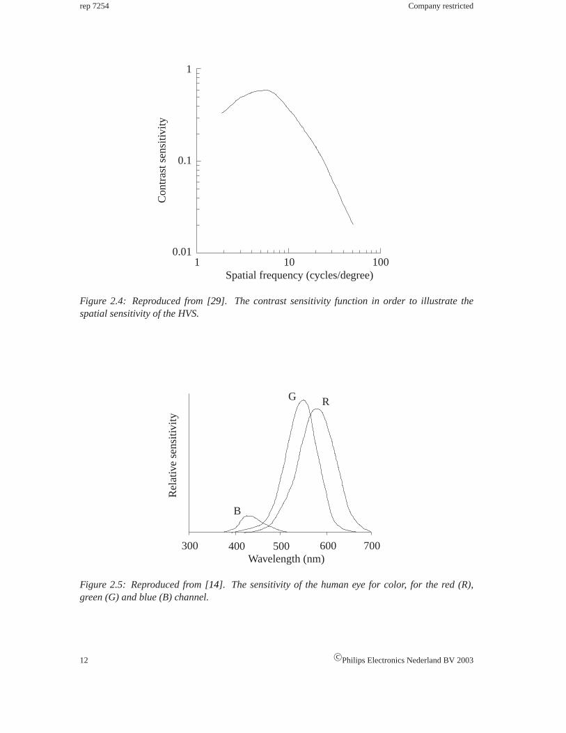
Spatial sensitivityis usually described by the sensitivity to contrast in luminance as a function ofspatial frequency, the result is the contrast sensitivity function, see Figure2.4. It can be seen thatthe human eye is most sensitive to luminance differences in the mid-frequencies and less sensitivefor the higher and lower frequencies.
The frequency sensitivityis illustrated with Figure2.5. The normal responses to the low, themiddle and the high frequencies, often called the blue, the green and the red channel, respectivelyare depicted. The human eye is significantly less sensitive for blue frequencies than it is for thered and green frequencies. Therefore, some watermarking methods embed a large proportion ofthe watermark in the blue channel of an RGB image.
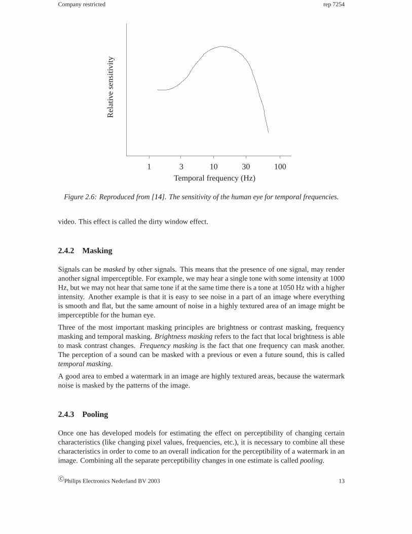
Figure2.6 shows thetemporal sensitivityfor the human eye. It can be seen that for frequenciesover 30 Hz, temporal sensitivity falls rapidly. This is why television and cinema frame rates arenot necessarily to be more than 60 frames per second. The total theory for temporal sensitivity isvery difficult, because the human eye follows moving objects. Temporal and spatial frequenciesare therefore partially converted into each other. A static watermark that is imperceptible in asingle video frame, can therefore be perceptible if more frames are shown after each other, like in
c©Philips Electronics Nederland BV 2003 11
rep 7254 Company restricted
Con
tras
tsen
sitiv
ity0.1
0.01
1
1 10 100Spatial frequency (cycles/degree)
Figure 2.4: Reproduced from [29]. The contrast sensitivity function in order to illustrate thespatial sensitivity of the HVS.
R
Rel
ativ
ese
nsiti
vity
G
B
300 400 500 600 700Wavelength (nm)
Figure 2.5: Reproduced from [14]. The sensitivity of the human eye for color, for the red (R),green (G) and blue (B) channel.
12 c©Philips Electronics Nederland BV 2003
Company restricted rep 7254
Temporal frequency (Hz)
1 3 10 30 100
Rel
ativ
ese
nsiti
vity
Figure 2.6: Reproduced from [14]. The sensitivity of the human eye for temporal frequencies.
video. This effect is called the dirty window effect.
2.4.2 Masking
Signals can bemaskedby other signals. This means that the presence of one signal, may renderanother signal imperceptible. For example, we may hear a single tone with some intensity at 1000Hz, but we may not hear that same tone if at the same time there is a tone at 1050 Hz with a higherintensity. Another example is that it is easy to see noise in a part of an image where everythingis smooth and flat, but the same amount of noise in a highly textured area of an image might beimperceptible for the human eye.
Three of the most important masking principles are brightness or contrast masking, frequencymasking and temporal masking.Brightness maskingrefers to the fact that local brightness is ableto mask contrast changes.Frequency maskingis the fact that one frequency can mask another.The perception of a sound can be masked with a previous or even a future sound, this is calledtemporal masking.
A good area to embed a watermark in an image are highly textured areas, because the watermarknoise is masked by the patterns of the image.
2.4.3 Pooling
Once one has developed models for estimating the effect on perceptibility of changing certaincharacteristics (like changing pixel values, frequencies, etc.), it is necessary to combine all thesecharacteristics in order to come to an overall indication for the perceptibility of a watermark in animage. Combining all the separate perceptibility changes in one estimate is calledpooling.
c©Philips Electronics Nederland BV 2003 13
rep 7254 Company restricted
2.5 Possible attacks on digital watermarks
As already mentioned, watermarks need to be robust against all kinds of attacks. A distinctionhas to be made between attacks directly on the watermark and targeted against other componentsof the watermarking system. For example, if it is relatively simple to remove or disconnect awatermark detection chip in a DVD-player, an attacker will focus his attention to this part of thesystem in order to reach his goal (in this case: to copy a DVD). In this section those kinds ofattacks are not considered, but the attention is focused on direct attacks on the watermarked data.An arrangement of attacks is given in Subsection2.5.1and some of the most common attacks arementioned in Subsection2.5.2- 2.5.4.
Some of the attacks mentioned in this section are considered to be normal processing, where othersare deliberate attacks.
2.5.1 Arrangement of attacks
Setyawan [32] gives a description and classification of different attacks. An overview can beextracted from his article and is given in Figure2.7.
From this figure it can be seen that a distinction is made between attacks aimed at the watermarkitself and attacks aimed at the host signal alone. The latter one can for example be used by anadversary wanting to change a watermarked image of a crime scene, because this image identifieshim as the perpetrator. His goal will be to change the watermarked image in such a way that hecan no longer be identified as the guilty person, but that it is not visible in the watermark that theimage has been altered.
Attacks on watermarks can be divided into three cases, namely attacks with the goal to remove thewatermark, synchronization attacks and ambiguity attacks, see Subsection2.5.2, 2.5.3and2.5.4respectively.
2.5.2 Removal attacks
Removal attackshave the goal to completely remove a watermark or damage a watermark to anextent that the watermark detector cannot detect it anymore. Generally, there are two types ofremoval attacks: one that processes the watermarked signal without analyzing it, and one thatanalyzes the watermarked signal in order to remove the watermark.
The first category, simple removal attacks, works both on the host signal and the watermark, andit affects the quality of both. Because the watermark energy is usually much lower than the hostsignal energy, the watermark is faster degraded than the host signal.
The second category, the analysis removal attacks, tries to analyze or estimate the watermark.After this analysis it is attempted to remove the watermark. These kinds of attacks are a lotsmarter than simple attacks, and they usually affect the watermark, but keep the host signal moreor less intact.
Examples of simple removal attacks are
Lossy compression: Examples of lossy compression techniques are JPEG (Joint PhotographicExperts Group: named after the committee that defined it) and MPEG (Motion PicturesExperts Group: data compression standard for motion-video and audio) compression. These
14 c©Philips Electronics Nederland BV 2003

Company restricted rep 7254
Attacks on watermarked data
Attacks aimed at the watermark
Removal attacks Synchronisation attacks
Simple removal
• Geometrical transformation
• Pixel deletion / substitution
• Mosaic attack
• Scramble / unscramble attack
Analysis removal
• Non-linear filtering
• Statistical averaging
• Collusion attacks
• Embedder / detector ob-servation
• Lossy compression
• Noise addition
• DA- & AD-conversion
• Transcoding
• General filtering
Attacks aimed at the host signal
Ambiquity attacks
Figure 2.7: An overview of possible attacks on a watermarked signal. This overview is based on[32]. Some of the attacks are normal processing and other deliberate attacks.
c©Philips Electronics Nederland BV 2003 15

rep 7254 Company restricted
techniques usually work on the parts of the data that are less important for the perceptualquality of the signal. Watermarking techniques usually also work in these parts, therefore itis likely that the watermark gets damaged due to lossy compression techniques.
Noise addition: The added noise is usually random and uncorrelated with the host signal and,more importantly, the watermark. Therefore it is unlikely that the noise affects the detectionof the watermark, unless the power of the noise is very high. In this case the perceptualquality of the watermarked signal is highly degraded, which is usually also unwanted by anattacker.
DA- & AD-conversion: Digital-to-Analog and Analog-to-Digital conversion takes place for ex-ample if a digital image is printed and then scanned again, or when a digital movie isrecorded on an analog videotape. In these cases the watermarked signal, and also the water-mark, is not completely the same as it was in the digital case. Some embedding techniques,like LSB modification (see Subsection2.6.2), are not robust against these degradations.
Transcoding: The process of going from one representation of data to another is called transcod-ing. Examples are going from a bitmap (BMP) image file to a GIF file (Graphics InterchangeFormat) and re-encoding an MPEG-stream into a higher or lower bit rate. This affects thewatermarked signal and the watermark could be damaged or even lost.
General filtering: General filtering techniques can be used to remove a watermark. Low passfiltering for example, might be able to remove a pseudo-random noise watermark, since thewatermark is essentially a high frequency noise [32].
Examples of analysis removal attacks are
Non-linear filtering: Using these techniques watermarks can be estimated and a watermark canbe removed by subtracting this estimate from the watermark data. In this way an estimatefrom the unwatermarked host signal is obtained.
Statistical averaging: If an attacker has a number of signals (images, video-frames), all water-marked with the same watermark, it is possible to average all images and extract an estimateof the watermark from this average. This only works if the watermarks are not dependent ofthe host signal.
Collusion attacks: In this case there are a number of copies of one host data, watermarked withdifferent watermarks. Combining all these copies, it is possible to estimate the original hostsignal by statistical averaging.
Embedder / detector analysis: An attacker possessing a watermark detector is able to look forthe smallest modifications made on the watermarked signal, which renders the watermarkundetectable. An attacker possessing a watermark embedder is able to watermark unwa-termarked material and obtaining the watermark by taking the difference. After this it ispossible to subtract the watermark from the original signal. If this modified host signalis then watermarked, the result is approximately the same as the original unwatermarkedmaterial.
16 c©Philips Electronics Nederland BV 2003
Company restricted rep 7254
2.5.3 Synchronization attacks
In the case ofsynchronization attacks, an attacker will not try to remove the watermark, but just toremove the synchronization with the detector, and in this way making a watermark undetectable.The quality of the image is to a large extent unchanged.
Examples of synchronization attacks are
Geometrical transformation: By simply shifting an image a few pixels to some direction (trans-lation), the watermark detector is unable to find the watermark (although it is still there),while the image remains largely unchanged. Other examples of geometrical transforma-tions are scaling, zooming, cropping and rotating.
Pixel deletion / substitution: It is possible to render a watermark undetectable by removing acomplete column of an image, or replacing it by another column. The image is still largelythe same after this operation.
Mosaic attack: With this attack an image is divided into smaller blocks. The detector will usuallyfail to detect a watermark in this smaller portion. The total image can still be represented byholding the smaller blocks together, like a mosaic.
Scramble / unscramble attack: It is used to bypass copy protection schemes in for exampleDVD-players. First the watermarked and illegal copy of a video is scrambled (mixed), thisscrambled copy is played on a DVD-player, which doesn’t recognize the watermark. Then,the copy is unscrambled in order to obtain the original copied video.
2.5.4 Ambiguity attacks
In the case ofambiguity attacksthe attacker simply tries to embed another watermark in the alreadywatermarked image. This way it is difficult for the detector to detect the original watermark.
2.6 Different watermarking techniques
Embedding a watermark can be done in a number of different ways. First of all it is possible tochange directly the pixel values of an image or a video frame, this is called embedding in thespatial domain. It is also possible to find a representation of a host signal in another domainand perform modifications on the coefficients in that domain. Examples of those domains are theDiscrete Fourier Transform (DFT) domain, the Discrete Cosine Transform (DCT) domain and thewavelet domain, see Subsection2.6.1.
When embedding a watermark in the DCT-domain, first the Discrete-Cosine-Transform is takenfrom the host signal, and then modifications are mode on the DCT-coefficients. The same holdsfor the other domains.
Making these modifications can also be done in a number of different ways. Well known tech-niques are Least Significant Bit (LSB) modification, noise-addition, Spread Spectrum techniques(for example the Patchwork algorithm), the reordering or deletion of coefficients, warping or mor-phing data parts, etc., see Subsection2.6.2- 2.6.4. Other watermarking processes are quantizationtechniques like Quantization Index Modulation (QIM), see Chapter3.
c©Philips Electronics Nederland BV 2003 17
rep 7254 Company restricted
Transformation
Embedder Y = X + W
x
X
W yInverseTransformation
m
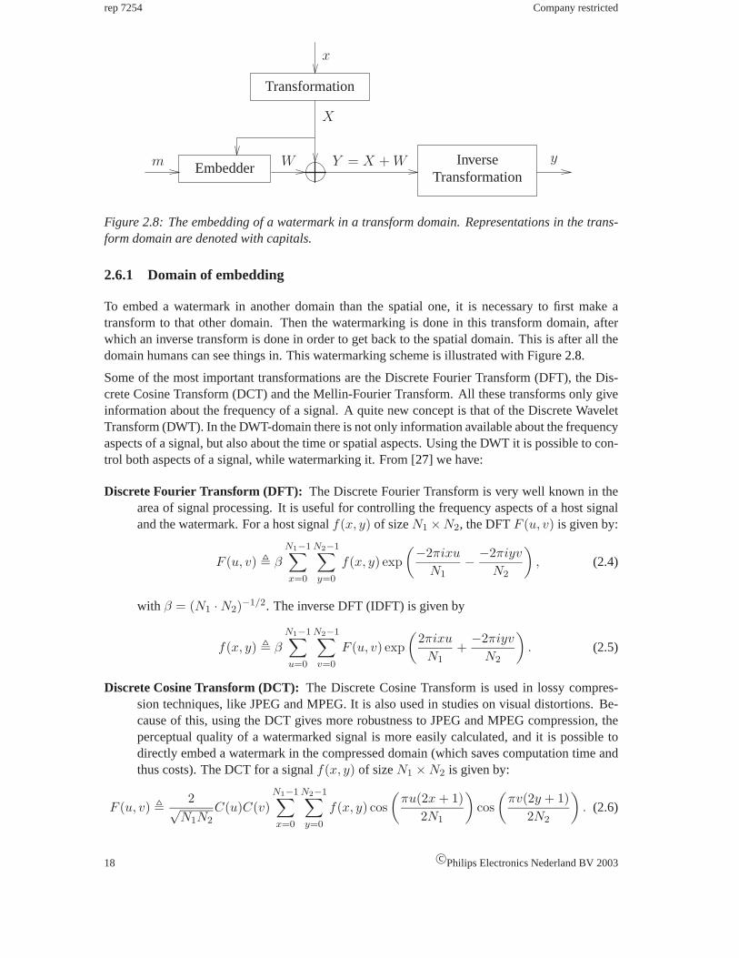
Figure 2.8: The embedding of a watermark in a transform domain. Representations in the trans-form domain are denoted with capitals.
2.6.1 Domain of embedding
To embed a watermark in another domain than the spatial one, it is necessary to first make atransform to that other domain. Then the watermarking is done in this transform domain, afterwhich an inverse transform is done in order to get back to the spatial domain. This is after all thedomain humans can see things in. This watermarking scheme is illustrated with Figure2.8.
Some of the most important transformations are the Discrete Fourier Transform (DFT), the Dis-crete Cosine Transform (DCT) and the Mellin-Fourier Transform. All these transforms only giveinformation about the frequency of a signal. A quite new concept is that of the Discrete WaveletTransform (DWT). In the DWT-domain there is not only information available about the frequencyaspects of a signal, but also about the time or spatial aspects. Using the DWT it is possible to con-trol both aspects of a signal, while watermarking it. From [27] we have:
Discrete Fourier Transform (DFT): The Discrete Fourier Transform is very well known in thearea of signal processing. It is useful for controlling the frequency aspects of a host signaland the watermark. For a host signalf(x, y) of sizeN1 ×N2, the DFTF (u, v) is given by:
F (u, v) � β
N1−1∑x=0
N2−1∑y=0
f(x, y) exp(−2πixu
N1− −2πiyv
N2
), (2.4)
with β = (N1 · N2)−1/2. The inverse DFT (IDFT) is given by
f(x, y) � β
N1−1∑u=0
N2−1∑v=0
F (u, v) exp(
2πixu
N1+
−2πiyv
N2
). (2.5)
Discrete Cosine Transform (DCT): The Discrete Cosine Transform is used in lossy compres-sion techniques, like JPEG and MPEG. It is also used in studies on visual distortions. Be-cause of this, using the DCT gives more robustness to JPEG and MPEG compression, theperceptual quality of a watermarked signal is more easily calculated, and it is possible todirectly embed a watermark in the compressed domain (which saves computation time andthus costs). The DCT for a signalf(x, y) of sizeN1 × N2 is given by:
F (u, v) � 2√N1N2
C(u)C(v)N1−1∑x=0
N2−1∑y=0
f(x, y) cos(
πu(2x + 1)2N1
)cos
(πv(2y + 1)
2N2
). (2.6)
18 c©Philips Electronics Nederland BV 2003
Company restricted rep 7254
whereC(u) = 12 for u = 0 andC(u) = 1
2
√2 otherwise. The inverse DCT (IDCT) is given
by
f(x, y) � 2√N1N2
N1−1∑u=0
N2−1∑v=0
C(u)C(v)F (u, v) cos(
πu(2x + 1)2N1
)cos
(πv(2y + 1)
2N2
).
(2.7)
Fourier-Mellin Transform: Most watermarking algorithm are not (very) robust against geomet-rical attacks, see Subsection2.5.3. TheFourier-Mellin Transformis based on the translationinvariance property of the Fourier transform:
f(x1 + a, x2 + b) ↔ F (u, v) exp (−i(au + bv)) . (2.8)
Use of this property, makes the watermark robust against a spatial shift. Robustness torotation and scaling (zoom) can be achieved by using a log-polar mapping:
(x, y) �→{
x = exp(ρ) cos(θ)y = exp(ρ) sin(θ)
with ρ ∈ R andθ ∈ [0, 2π], (2.9)
whereR is the set of possible scale-factors. This way, a rotation results in a translation inthe logarithmic coordinate system and a zoom results in a translation in the polar coordinatesystem.
2.6.2 Least Significant Bit (LSB) modification
Pixels in an image or a video frame are usually represented by an 8-bit number (0 - 255 inZ255).Modifying the last bit from a pixel results in the addition of±1 in Z255. This modification isso small, that it is very difficult to see in the image or video frame. Because modifying this lastbit introduces the smallest possible distortion, it is called the Least Significant Bit (LSB). A verysimple way of embedding a binary message in an image is by modifying the LSB such that it isequal to the message bit. This way it is possible to embed a message bit in every pixel, so thepayload of this method is very high. But the drawback is that it is not very robust: changing theLSB’s by a random pattern, completely removes the watermark. Therefore the capacity is verylow.
2.6.3 Spread Spectrum techniques
The embedding of a watermark usingSpread Spectrum(SS) techniques, consist of the adding of apseudo-random noise patternp to a host signal:
y = x + p. (2.10)
The detection is based on correlation. The correlation of the watermarked signaly with the knownpatternp is determined. If the correlation is above some thresholdT , it is assumed that the water-marked signal was indeed watermarked with patternp:
〈y, p〉 = 〈x + p, p〉 = 〈x, p〉 + 〈p, p〉 ≈ 〈p, p〉 (2.11)
≈{
1 if p = p
1 otherwise, (2.12)
c©Philips Electronics Nederland BV 2003 19
rep 7254 Company restricted
where the first approximation comes from the fact that the pseudo-random noise patternp and thehost signalx are highly uncorrelated, and the second approximation follows from the definition ofthe correlation coefficient.
This Spread Spectrum technique is highly robust against simple attacks, but it is only possible toembed one bit: watermark or no watermark. It is possible to embed more than one bit into a hostsignal by dividing the host signal into smaller subsamples and embed one bit in each part. Thiswill come at the cost of some robustness. If an image is cropped, bits will get lost.
Another way to embed more than one bit into a host signal is by using a technique called DirectSequence Code Division Multiple Access (DS-CDMA) Spread Spectrum communication. Whereas normal Spread Spectrum adds only one pattern, DS-CDMA Spread Spectrum uses more thanone (N ) patterns. The embedding is then:
y = x +N∑
i=1
βipi, (2.13)
where
βi =
{+1 if message bit= 0−1 if message bit= 1
. (2.14)
Detection is again done by correlation. The decision rule for patterni is:
E [(pi − Epi)(y − Ey)] =
{> 0 then a 0 is detected
< 0 then a 1 is detected. (2.15)
This DS-CDMA Spread Spectrum technique is (to some amount) robust against cropping, butthere is some interference between the watermark patterns.
2.6.4 Patchwork Algorithm
A very simple example of a Spread Spectrum watermarking method is thePatchwork algorithm.The pseudo-random pattern used here consists of±1’s.
The Patchwork algorithm divides an image into two setsA andB. To embed 0, the values of thepixels in setA are raised by 1 and the values of the pixels in setB are lowered by 1. In order toembed 1, the values of the pixels in setA are lowered instead of raised and that ofB raised insteadof lowered. Let’s say that the setsA andB both have the sizeN . Detection is done by comparingthe differenceD of the averagesyA andyB of setA andB. If a watermark is embedded (in thiscase a 0), this detection looks like:
D = yA − yB =1N
∑y∈A
yi − 1N
∑y∈B
yi =1N
∑x∈A
(xi + 1) − 1N
∑x∈B
(xi − 1)
= xA − xB + 2 ≈ 2, (2.16)
where it is assumed that the average of pixel values in setA equals that of setB. If a 1 is embeddedyA − yB ≈ −2 and if nothing is embeddedyA − yB ≈ 0.
20 c©Philips Electronics Nederland BV 2003

Company restricted rep 7254
A thresholdT ∈]0, 2[ can be set, and the decision rule for the detected message bitm is:
m =
1 if D < −T
nothing if−T ≤ D ≤ T
0 if D > T
. (2.17)
The precise form of the setsA andB is the secret of the watermark embedders.
c©Philips Electronics Nederland BV 2003 21

rep 7254 Company restricted
22 c©Philips Electronics Nederland BV 2003

Chapter 3
Quantization Watermarking
As seen in Section2.6, watermarking can be done using several techniques. The focus of thisreport is on quantization watermarking. In this chapter we will explain the basics of quantizationbased watermarking methods. As seen before, a watermarking process consists of the embeddingof a watermark in a host signal, the transmission of the watermarked signal over a channel mod-elling the attacks, and the subsequent detection. Because in practice the host signal is not availablefor comparison at the detector, only blind detection is considered (see Subsection2.3.7). The de-tection of the watermark at the detector is influenced by the host signal, this is calledhost signalinterference. At the embedder the host signal is known. It is possible to use this information inorder to reduce the host signal interference on detection. The principle of using the host signalat the embedder is known as usingside information at the encoder, a concept of Claude Shannon[34].
Costa [11] considered this principle for an Additive White Gaussian Noise (AWGN) channel andan i.i.d. Gaussian host signal. See Figure2.1, where the noisen is i.i.d. Gaussian noise. Costaproposed a blind scheme that performs as well as a non-blind scheme, i.e., the detection perfor-mance cannot be improved by giving the detector access to the original data. Host interferenceat the decoder is completely absent. Chen and Wornell rediscovered the paper of Costa [11] andintroduced the principle of using side information at the encoder into the world of watermarking.The so-called Ideal Costa Scheme (ICS) is discussed in Section3.1.
It was shown by Chen and Wornell that their previously proposed watermarking scheme [3, 4, 5, 6]based on the so-called Quantization Index Modulation (QIM) scheme, can be explained in terms ofCosta’s scheme. An extended version of QIM, distortion compensated QIM (DC-QIM), performsas well as the Costa scheme. In Section3.2QIM and DC-QIM are discussed.
The Costa scheme is not practical, as will be seen in Section3.1, and therefore attention is paid tosome practical implementation of the ICS, the so-called Scalar Costa Scheme (SCS), developedby Eggers et al. [15, 17, 18]. This scheme is considered in Section3.3.
This report is focussed on binary dithered quantization, which is a simple case of the SCS orDC-QIM. The resulting scheme is explained in simple terms in Section3.4.
In Section3.5and3.6the principles of embedding and detecting a message are treated.
The performance judgement of the different schemes is based on information theoretic notionsof capacity, rate and distortion. Good books on this subject are [12, 25]. Basic knowledge oninformation theory is assumed.
23

rep 7254 Company restricted
search inUNm search inUN
w
α
-u0m
x
y = x + w
n
r m
Embedder Detector
Figure 3.1: Costa’s scheme. Partially reproduced from [18]. Compare with Figure2.1.
3.1 The Ideal Costa Scheme
The communications problem, as depicted in Figure2.1, is to retrieve the messagem embeddedin a host signalx at the detector. Costa assumed that the host signalx and the noise signaln areof lengthN and i.i.d. Gaussian distributed, i.e.,x ∼ N(0, σ2
xIN ) andn ∼ N(0, σ2nIN ). The
interfering Gaussian noisesx andn are not known at the decoder. The encoder, however, knowsx.
At the encoder, the watermarked signal is chosen depending on the messagem, the side infor-mationx and realizationsu of an auxiliary random variableU . Appropriate realizationsu of Ufor all possible messagesm and all possible side informationx are listed in a codebookU . Thewatermarkw has a lengthN equal to the length of the host signal.
In order to solve this communications problem, Costa introduced anN -dimensional random code-bookUN with codewordsu
UN �{
u(p) = ω(p) + αχ(p) | p ∈ {1, 2, · · · , P},
W ∼ N(0, σ2
W IN
), X ∼ N
(0, σ2
XIN
)},
(3.1)
whereω(p) andχ(p) are realizations of twoN -dimensional independent random processesW andX with Gaussian pdf, andα a real codebook parameter, with0 ≤ α ≤ 1. The size of the codebook,i.e., the number of codewords, is given byP , typically a large number. So the codebookUN isreally a random codebook, containingP codewords of lengthN .
In the limit asN → ∞, Costa’s codebookUN achieves the capacity of communication with i.i.d.Gaussian side informationx both at the encoder and decoder and an AWGN channel. See [11, 18]for more details on the Ideal Costa Scheme.
The codebook is partitioned intoM disjoint sub-codebooks, withM the number of possible wa-termark messages. Partitioning is done such that each sub-codebookUN
m contains about the samenumber of codeword sequences. SoUN = UN
1 ∪UN2 ∪ · · · ∪UN
M . This codebook is available bothat the encoder and decoder. See also Figure3.1.
According to [18] the embedding of a messagem into the host signalx is equivalent to finding asequenceu0 in the setUN
m such thatw = u0 − αx is nearly orthogonal in the Euclidean sense to
24 c©Philips Electronics Nederland BV 2003

Company restricted rep 7254
x. If the length of the codewordsN goes to infinity the probability that no such sequenceu0 exist,goes to zero exponentially.
Subsequently, the watermarked signaly = x+w = (1−α)x+u0 is transmitted over the AWGNchannel and the received signal isr = y + n.
Decoding is done by finding a sequenceu in the entire codebookUN such thatu − αr is nearlyorthogonal tor. The probability that there is only one such sequenceu0 is high if N goes toinfinity. The indexm of the sub-codebookUN
m containingu is the decoded message.
Costa showed that for the codebook (3.1), for N → ∞, and with optimal parameterα∗, with
α∗ =σ2
w
σ2w + σ2
n
=1
1 + 10−WNR/10, (3.2)
the capacity is
CICS =12
log(
1 +σ2
w
σ2n
), (3.3)
which is equal to the capacity of the transmission scenario where the host signalx is known to thedecoder [18]. So the Costa scheme is optimal in the sense that it is capacity achieving. Here theWNR is theWatermark-to-Noise Ratiowhich is defined as
WNR � 10 log10
(σ2
w
σ2n
). (3.4)
So, not knowing the host signal at the decoder does not decrease capacity. Note that the capacitydepends only on the WNR and is independent fromx. Also note that this capacity is only achievedfor a huge random codebook size, therefore this is not a practical way of achieving full capacity.
3.2 Quantization Index Modulation
Chen and Wornell proposed a watermarking scheme which they called Quantization Index Mod-ulation. They showed that this scheme is a special case of the Ideal Costa Scheme [6, 7]; QIMis ICS withα = 1. They also showed that QIM is not capacity achieving compared to the ICS,but in fact close. Therefore they proposed an improvement of QIM, which they called DistortionCompensated QIM (DC-QIM). This DC-QIM scheme is in fact equal to the ICS and thereforeoptimal. The principle of QIM is explained in Subsection3.2.1and the extension of this scheme(DC-QIM) is treated in Subsection3.2.2.
3.2.1 Quantization Index Modulation
Chen and Wornell view the embedding functiony = s(x; m) as an ensemble of functions of thehost signalx, indexed by the messagem. For the distortion to be small it is required thaty andxare close in distance, sos(x; m) ≈ x, ∀m. For this system to be robust it is required that the em-bedding functions are far away in some sense for different messages, sod(s(x; mi), s(x, mj)) �0, ∀i, j, i �= j, with d(u, v) some distance measure. At least the ranges should be non-intersecting,because else there will be some values ofs from which it is not possible to uniquely determinem.
c©Philips Electronics Nederland BV 2003 25
rep 7254 Company restricted
dmin
©
©
©
©
©©
×
= 1 level
×
×
××
×
©× = 0 level
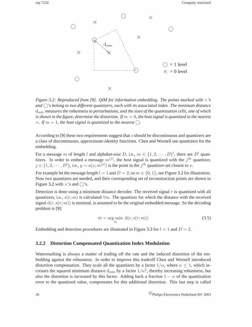
Figure 3.2: Reproduced from [9]. QIM for information embedding. The points marked with×’sand©’s belong to two different quantizers, each with its associated index. The minimum distancedmin measures the robustness to perturbations, and the sizes of the quantization cells, one of whichis shown in the figure, determine the distortion. Ifm = 0, the host signal is quantized to the nearest×. If m = 1, the host signal is quantized to the nearest©.
According to [9] these two requirements suggest thats should be discontinuous and quantizers area class of discontinuous, approximate-identity functions. Chen and Wornell use quantizers for theembedding.
For a messagem of lengthl and alphabet-sizeD, i.e., m ∈ {1, 2, · · · , D}l, there areDl quan-tizers. In order to embed a messagem(j), the host signal is quantized with thejth quantizer,j ∈ {1, 2, · · · , Dl}, i.e.,y = s(x; m(j)) is the point in thejth quantizer-set closest tox.
For example let the message lengthl = 1 andD = 2, som ∈ {0, 1}, see Figure3.2for illustration.Now two quantizers are needed, and their corresponding set of reconstruction points are shown inFigure3.2with ×’s and©’s.
Detection is done using a minimum distance decoder. The received signalr is quantized with allquantizers, i.e.,s(r; m) is calculated∀m. The quantizer for which the distance with the receivedsignald(r, s(r; m)) is minimal, is assumed to be the original embedded message. So the decodingproblem is [9]:
m = arg minm
d(r, s(r; m)) (3.5)
Embedding and detection procedures are illustrated in Figure3.3for l = 1 andD = 2.
3.2.2 Distortion Compensated Quantization Index Modulation
Watermarking is always a matter of trading off the rate and the induced distortion of the em-bedding against the robustness. In order to improve this tradeoff Chen and Wornell introduceddistortion compensation. They scale all the quantizers by a factor1/α, whereα ≤ 1, which in-creases the squared minimum distancedmin by a factor1/α2, thereby increasing robustness, butalso the distortion is increased by this factor. Adding back a fraction1 − α of the quantizationerror to the quantized value, compensates for this additional distortion. This last step is called
26 c©Philips Electronics Nederland BV 2003
Company restricted rep 7254
©
©
©
©
©©
× ×
= 0 level
×
××
×
r embedding
detectingy
x©×
= 1 level
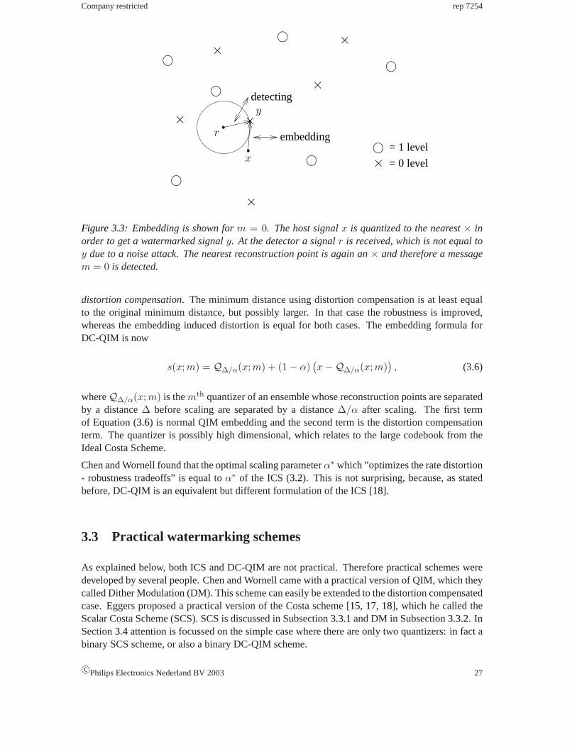
Figure 3.3: Embedding is shown form = 0. The host signalx is quantized to the nearest× inorder to get a watermarked signaly. At the detector a signalr is received, which is not equal toy due to a noise attack. The nearest reconstruction point is again an× and therefore a messagem = 0 is detected.
distortion compensation. The minimum distance using distortion compensation is at least equalto the original minimum distance, but possibly larger. In that case the robustness is improved,whereas the embedding induced distortion is equal for both cases. The embedding formula forDC-QIM is now
s(x; m) = Q∆/α(x; m) + (1 − α)(x −Q∆/α(x; m)
), (3.6)
whereQ∆/α(x; m) is themth quantizer of an ensemble whose reconstruction points are separatedby a distance∆ before scaling are separated by a distance∆/α after scaling. The first termof Equation (3.6) is normal QIM embedding and the second term is the distortion compensationterm. The quantizer is possibly high dimensional, which relates to the large codebook from theIdeal Costa Scheme.
Chen and Wornell found that the optimal scaling parameterα∗ which ”optimizes the rate distortion- robustness tradeoffs” is equal toα∗ of the ICS (3.2). This is not surprising, because, as statedbefore, DC-QIM is an equivalent but different formulation of the ICS [18].
3.3 Practical watermarking schemes
As explained below, both ICS and DC-QIM are not practical. Therefore practical schemes weredeveloped by several people. Chen and Wornell came with a practical version of QIM, which theycalled Dither Modulation (DM). This scheme can easily be extended to the distortion compensatedcase. Eggers proposed a practical version of the Costa scheme [15, 17, 18], which he called theScalar Costa Scheme (SCS). SCS is discussed in Subsection3.3.1and DM in Subsection3.3.2. InSection3.4attention is focussed on the simple case where there are only two quantizers: in fact abinary SCS scheme, or also a binary DC-QIM scheme.
c©Philips Electronics Nederland BV 2003 27

rep 7254 Company restricted
3.3.1 The Scalar Costa Scheme
The reason why the Costa scheme is not practical, is the used huge random codebook. Searchingthis codebook is comprehensive because of the size and because there is no structure on thiscodebook. Therefore Eggers proposed to use a suboptimal, structured codebook, without changingthe main concept of Costa’s idea. Eggers called this scheme the Scalar Costa Scheme (SCS). LikeCosta’s scheme, this scheme is also independent from the host signal, because a random keysequenced is used.
The codebookUN of Costa, see Equation (3.1), is structured by Eggers as a product codebookUN = U1 ⊗ U1 ⊗ · · · ⊗ U1 of N identical one-dimensional component codebooks. Because ofthe use of the one-dimensional (scalar) component codebooks, Eggers refers to this watermarkingscheme as the ScalarCosta Scheme. The one-dimensional component codebooksU1 are separatedinto D disjoint parts, whereD is the size of the alphabetD = {0, 1, · · · , D − 1}. SoU1 =U1
0 ∪ U11 ∪ · · · ∪ U1
D−1. Taking a product codebook is equivalent with sample wise quantization.Separating the one-dimensional component codebookU1 is equivalent with using quantizers thatare shifted versions of each other. The one-dimensional codebookU1 with the use of a secret keyd is chosen to be
U1(α, ∆, D, d) ={
u = (k + d)α∆ + mα∆D
| m ∈ D, k ∈ Z
}(3.7)
and themth sub-codebook is given by
U1m(α, ∆, D, d) =
{u = (k + d)α∆ + m
α∆D
| k ∈ Z
}, (3.8)
where∆ is the step size used for quantization. Without knowingd it is impossible to reconstructthe codebookUN used for the watermark embedding.
Using the product codebook is equivalent to calculating the quantization sample-wise, i.e., foreachn ∈ {1, 2, · · · , N} calculate
qn = Q∆
{xn − ∆
(mn
D+ dn
)}−(xn − ∆
(mn
D+ dn
)), (3.9)
whereQ∆{·} denotes scalar uniform quantization with step size∆, soQ∆{z} =⌊
z∆
⌉∆, with
�·� rounding to the nearest integer. The watermark is then given byw = αq and the watermarkedsignal isy = x + w = x + αq.
It is shown in [20, 24, 31] that for a uniformly distributed key sequenced thatq andw are statisti-cally independent fromx.
Eggers gives the following relation betweenα, the quantization step size∆ and the watermarkpowerσ2
w:
α =σw
√12
∆. (3.10)
Because this scheme is suboptimal, the capacity will be lower than the Costa capacity, see Equation(3.3). Also the value of the optimalα∗ will be different. Eggers found a numerical solution forthis optimalα∗. However, no analytical solution has been found yet [8]. In Chapter8 we will givean implicit analytical expression for the optimalα∗.
SCS decoding is similar to ICS decoding as described in Section3.1, except that a different code-book is used. If the product codebookUN is treated as a quantizer, than decoding is equivalent toquantizing the received valuer to the closest codeword.
28 c©Philips Electronics Nederland BV 2003

Company restricted rep 7254
3.3.2 Dither Modulation
Embedding using quantization and a dither signald gives an embedding functions(x; m) = q(x+d)−d. In [9] Chen and Wornell give some practical examples of Dither Modulation: Coded BinaryDither Modulation with Uniform Scalar Quantization and Spread-Transform Dither Modulation.See this article for more details.
3.4 Embedding by binary dithered quantization with uniform quan-tization step size
This report focuses on the case of binary dithered quantization with uniform quantization stepsize. Binary means that the alphabetD has size 2, soD = {0, 1}. This means that the messagem consists of 0’s and 1’s only; The message is considered to be a binary message. Ditheredquantization means that the quantization cells and reconstruction points are shifted versions ofeach other, it is the same as saying that Dither Modulation is used. A uniform quantization stepsize refers to the fact that the reconstruction points are uniformly spread over the quantizationspace.
This section gives a simple explanation of the workings of a watermarking embedding algorithmthat uses the principles of the SCS, or a practical implementation of DC-QIM. In Subsection3.4.1the basic watermarking scheme, without dither and distortion compensation, is given. The princi-ple of dithering is further explained in Subsection3.4.2and distortion compensation is treated inSubsection3.4.3.
In this report the watermarking of images is considered, so the host signalx is in fact an image.It is convenient to view an image as a matrix of pixel values, where the pixel values represent theintensity or the color of a pixel.
For the case of an 8 bit grey-scale image, every pixel consists of one value in the setZ255 � {z ∈Z | 0 ≤ z ≤ 255}, representing the luminance. For an 8 bit color image, every pixel consistsof three values, representing either red, green and blue color intensities (for an RGB image), orone luminance and two chrominance values (for a YUV image). Each of these values are againin the setZ255. From now on, when we talk about changing a pixel value, we mean changingthe luminance value. An RGB image and a YUV image are linearly related and can be simplyconverted into each other.
3.4.1 The basic scheme
A messagem is a sequence of bits of a certain length, sayl (So,m ∈ {0, 1}l). It is possible toembed a message bitmi, i ∈ {1, 2, · · · , l}, in a pixel of choice with valuexj , j ∈ {1, 2, · · · , N}.Using QIM, pixels are quantized to values in the set{z ∈ Z255 | z = k
2∆, k ∈ Z}. So the valueof a pixel is no longer represented by the values in the setZ255, but by fewer values. The valuesin the new set are called the quantization levels. A level with valuek∆, k ∈ Z is associated withmessage bit 0 and is defined to be an even level. The levels associated with 1 are shifted versionsof the even levels, they are shifted by∆/2. These levels have a value(k + 1
2)∆, k ∈ Z and aredefined to be odd levels. Here,∆ represents the minimal distance between two equal levels, so theminimal distance between two odd or two even levels, and is called thequantization step size. SeeFigure3.4.
c©Philips Electronics Nederland BV 2003 29
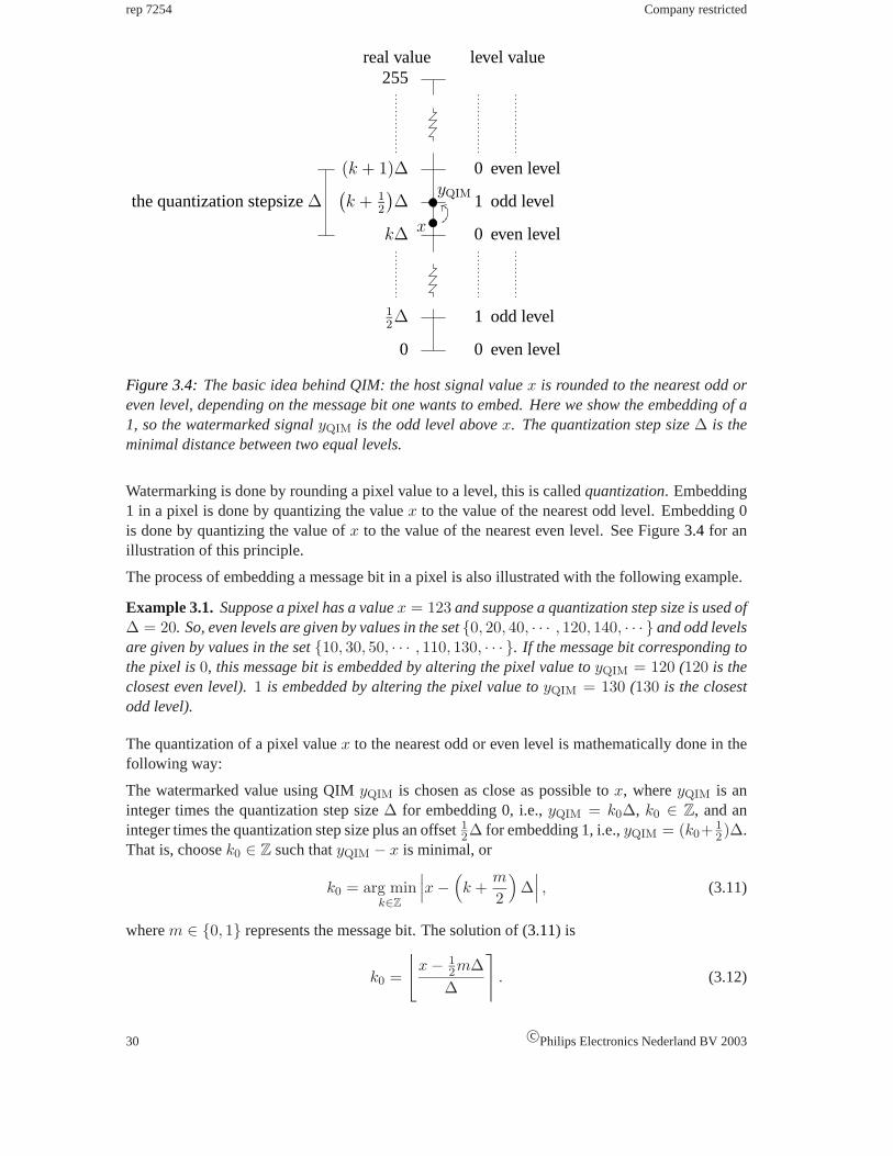
rep 7254 Company restricted
(k + 1
2
)∆
0 even level
1 odd level
0 even level
(k + 1)∆
255
x
real value level value
yQIM
0 0 even level
1 odd level12∆
k∆
the quantization stepsize∆
Figure 3.4: The basic idea behind QIM: the host signal valuex is rounded to the nearest odd oreven level, depending on the message bit one wants to embed. Here we show the embedding of a1, so the watermarked signalyQIM is the odd level abovex. The quantization step size∆ is theminimal distance between two equal levels.
Watermarking is done by rounding a pixel value to a level, this is calledquantization. Embedding1 in a pixel is done by quantizing the valuex to the value of the nearest odd level. Embedding 0is done by quantizing the value ofx to the value of the nearest even level. See Figure3.4 for anillustration of this principle.
The process of embedding a message bit in a pixel is also illustrated with the following example.
Example 3.1. Suppose a pixel has a valuex = 123 and suppose a quantization step size is used of∆ = 20. So, even levels are given by values in the set{0, 20, 40, · · · , 120, 140, · · · } and odd levelsare given by values in the set{10, 30, 50, · · · , 110, 130, · · · }. If the message bit corresponding tothe pixel is0, this message bit is embedded by altering the pixel value toyQIM = 120 (120 is theclosest even level).1 is embedded by altering the pixel value toyQIM = 130 (130 is the closestodd level).
The quantization of a pixel valuex to the nearest odd or even level is mathematically done in thefollowing way:
The watermarked value using QIMyQIM is chosen as close as possible tox, whereyQIM is aninteger times the quantization step size∆ for embedding 0, i.e.,yQIM = k0∆, k0 ∈ Z, and aninteger times the quantization step size plus an offset1
2∆ for embedding 1, i.e.,yQIM = (k0+ 12)∆.
That is, choosek0 ∈ Z such thatyQIM − x is minimal, or
k0 = arg mink∈Z
∣∣∣x −(k +
m
2
)∆∣∣∣ , (3.11)
wherem ∈ {0, 1} represents the message bit. The solution of (3.11) is
k0 =
⌊x − 1
2m∆∆
⌉. (3.12)
30 c©Philips Electronics Nederland BV 2003
Company restricted rep 7254
So for each pixel we have the codebook
U1 (∆) ={
u =(k +
m
2
)∆ | m ∈ {0, 1}, k ∈ Z
}. (3.13)
Compare this with the component codebook of Eggers, withα = 1, D = {0, 1}, soD = 2, andd = 0, see Equation (3.7).
Consequently, the embedding formula of the basic QIM scheme becomes
yQIM =(k0 +
m
2
)∆ =
⌊x − 1
2m∆∆
⌉∆ +
m∆2
, (3.14)
which can be compared withy = x + αq, with q as in (3.9), for α = 1, D = 2 andd = 0.
Example 3.2. (Continued) The watermarked pixel valueyQIM using QIM can also be calculated
using Equation (3.14). Then we haveyQIM =⌊
123− 12m·20
20
⌉· 20 + m·20
2 , which givesyQIM = 120for m = 0 andyQIM = 130 for m = 1.
3.4.2 Dithering
As said before, embedding information in every pixel of an image using QIM, causes every pixelto have a value a multiple of half the quantization step size. This way the statistics of an imageare changed. This is undesirable, because a watermarked image should be difficult to distinguishfrom the original one. It is very easy to find out what the quantization levels are and what thequantization step size∆ is, just by drawing a histogram of the pixel values of the watermarkedimage; The values will be centered around the quantization levels. This is illustrated by Figure3.5. Information about the quantization levels can be used to remove the watermark. For securityreasons it is undesirable to reveal this information and for perceptibility reasons it is undesirableto change the image statistics.
Another disadvantage of the above described basic scheme is the appearance of contour lines inthe watermarked imageyQIM. While in the original image a smooth change to another color canbe seen, in the watermarked image these changes will go with jumps; The bigger the quantizationstep size∆, the bigger the jumps. This is illustrated with Figure3.6.
These disadvantages can be overcome by introducingdither. Dither shifts the levels by a valued,so nowy = k∆ + d, where the ditherd is chosen differently for different pixels. The quantizationprocedure is now to first add a valued to the original pixel valuex, then quantize this new valuex + d to the nearest odd or even level and finally subtract the ditherd again. This kind of dither iscalledsubtractive dither.
As said before, for every pixel a different dither value is chosen. This way, the contour linesdisappear, giving the watermarked image better perceptual quality. This effect can be seen inFigure3.6. We have watermarked the monarch image with parameter∆ = 35. Because ditheradds different values to different pixels, the values of the watermarked image will be no longercentered around the levels. It is not possible anymore to know what the quantization levels are byanalyzing the watermarked image (See Figure3.5).
The new quantization formula using QIM with dithering is now (for comparison see Equation(3.14)):
c©Philips Electronics Nederland BV 2003 31

rep 7254 Company restricted
0 50 100 150 200 250
(a) Histogram of original imagemonarch.bmp
0 50 100 150 200 250
(b) Histogram of the watermarked imagemonarch.bmp using the basic QIM schemewithout dither modulation.
0 50 100 150 200 250
(c) Histogram of the watermarked imagemonarch.bmp using the basic QIM schemewith dither modulation.
Figure 3.5: The effect of dither: Using the basic QIM scheme quantization levels can be readoff easily (Subfigure3.5(b)); This is not possible anymore using dither modulation (Subfigure3.5(c)). Watermarking is done here using QIM (with or without dither) with a quantization stepsize∆ = 35. This is taken quite large, for illustrative reasons. Histogram3.5(c)does not resemblehistogram3.5(a)in this case, because the large∆ causes a large distortion.
yQIM+d =
⌊x + d − 1
2m∆∆
⌉∆ − d +
m∆2
. (3.15)
Compare Equation (3.15) with the watermarking formula given in Equation (3.9), with α = 1.For a uniformly distributed dither sequence the watermarkw is statistically independent from thehost signalx. The dither sequence must be known at the embedder and the detector. Thereforethe dither sequence is determined in advance. Following Chen [8] the dither is chosen uniformlydistributed over the range[−1
4∆, 14∆].
At the detector the dither sequence is first added to the received image before proceeding with thedetection process. The detection procedure is explained in Section3.6.
32 c©Philips Electronics Nederland BV 2003

Company restricted rep 7254
(a) Original imagemonarch.bmp
(b) Watermarked image using the basic QIM schemewithout dither modulation.
(c) Watermarked image using the basic QIM schemewith dither modulation.
Figure 3.6: The effect of dither: Contour lines, introduced by the basic QIM scheme (Subfigure3.6(b)), disappear with dither modulation (Subfigure3.6(c)). Watermarking is done using a largequantization step size∆ = 35.
3.4.3 Distortion compensation
In Subsection3.2.2distortion compensation is treated. For the case of the practical scheme thismeans that part of the watermarking errorε = y − x is added back:
ySCS = x + αε = x + α (yQIM+d − x) , (3.16)
where0 ≤ α ≤ 1. The watermarking formula for QIM with dithering and distortion compensationis now:
ySCS = x + α
(⌊x + d − 1
2m∆∆
⌉∆ − d +
m∆2
− x
). (3.17)
This embedding formula can be compared to the codebook of the SCS, see Equation (3.7). It isclear that (3.17) equals the SCS of Eggers, wherey = x + αq, with q given in Equation (3.9).
This process of bringing down the quantization error is illustrated in Figure3.7. Using it willreduce the watermark distortion, but decrease robustness, as smaller changes are more difficultto notice. Chen and Wornell [9] propose to use distortion compensation, as it can improve theachievable rate distortion-robustness tradeoffs of QIM methods.
Now there are two parameters to control the robustness and the perceptibility of the watermark,namely the quantization step size∆ and the distortion compensation parameterα. That is, the
c©Philips Electronics Nederland BV 2003 33

rep 7254 Company restricted
0 1 0
0 1 0
x
∆
Q∆(x)
y
α = 0
α = 0.75
α = 1
Figure 3.7: The process of distortion compensation. The upper line represents the value of thehost signalx. Without distortion compensation (α = 1) and dithering, all values are quantizedto an odd or even level with a functionQ∆(x; m) and the watermarked signal equalsQ∆(x; m).With distortion compensation(α ∈]0, 1[) a part of the quantization error is returned and the wa-termarked signal equalsy.
distortionD(α, ∆) and the robustness are determined byα and∆.
In order to begin embedding, one has to know the embedding parameter pair(α, ∆). The readermay wonder whether it is possible to simply choose a pair(1, ∆) and do just as well as the case(α, ∆/α), i.e., embedding using QIM versus embedding using DC-QIM.
In both cases the distortion introduced by the watermark will beα2∆2
12 . Is the robustness betterfor QIM? It is made clear intuitively by Figure3.8 that for equal distortion, DC-QIM has a largerminimal distance, and thus a larger robustness. This can also be seen as follows, see Figure3.7for reference. Supposex is uniformly distributed over the range of a quantization bin. For thecase of QIM with parameters(1, ∆) x is quantized to a quantization level. The distance from thislevel to the nearest wrong level is given bydQIM = 1
2∆. For the case of DC-QIM with parameters(α, ∆/α), the watermarked valuey is within (1 − α)1
2∆α of a quantization level. On averagey is
12(1 − α)1
2∆α from this level, becausey is also uniformly distributed. The distance to the nearest
wrong level is given bydDC−QIM = 12
∆α − 1
2(1−α) ∆2α = 1
4(∆α +∆). We havedDC−QIM > dQIM
for α < 1, so DC-QIM performs better on average.
In Chapter8 it is shown that DC-QIM with parameterα ∈]0, 1] is usually better than QIM withα = 1, by minimizing the bit error probability.
3.5 Spreading a message and repetition coding
Equation (3.17) defines a watermark embedding algorithm. In this section this algorithm is appliedon digital images. It is assumed in this section that an image is a matrix of luminance-values ofsizeN × M , so the hostx is N × M . A messagem is a series of bits of lengthl and is givenbeforehand.
If the size of a messagel equals the number of image pixelsN × M , then each message bitmi,i ∈ {0, 1, · · · , l} is associated with one pixelxij , i ∈ {0, 1, · · · , N}, j ∈ {0, 1, · · · , M} in a
34 c©Philips Electronics Nederland BV 2003
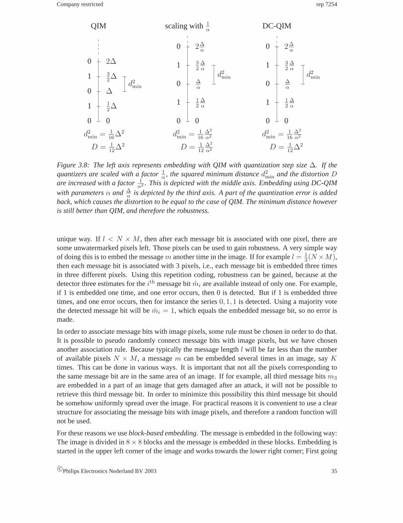
Company restricted rep 7254
0
1
0
1
0 2∆
∆
QIM
32∆
0
12∆
d2min = 1
16∆2
0 0
0
1
0
1 12
∆α
∆α
32
∆α
2∆α
d2min = 1
16∆2
α2
0 0
0
1
0
1 12
∆α
∆α
32
∆α
2∆α
d2min = 1
16∆2
α2
D = 112
∆2 D = 112
∆2
α2 D = 112
∆2
d2min
d2min d2
min
DC-QIMscaling with 1α
Figure 3.8: The left axis represents embedding with QIM with quantization step size∆. If thequantizers are scaled with a factor1α , the squared minimum distanced2
min and the distortionDare increased with a factor1
α2 . This is depicted with the middle axis. Embedding using DC-QIMwith parametersα and ∆
α is depicted by the third axis. A part of the quantization error is addedback, which causes the distortion to be equal to the case of QIM. The minimum distance howeveris still better than QIM, and therefore the robustness.
unique way. Ifl < N × M , then after each message bit is associated with one pixel, there aresome unwatermarked pixels left. Those pixels can be used to gain robustness. A very simple wayof doing this is to embed the messagem another time in the image. If for examplel = 1
3(N ×M),then each message bit is associated with 3 pixels, i.e., each message bit is embedded three timesin three different pixels. Using this repetition coding, robustness can be gained, because at thedetector three estimates for theith message bitmi are available instead of only one. For example,if 1 is embedded one time, and one error occurs, then 0 is detected. But if 1 is embedded threetimes, and one error occurs, then for instance the series0, 1, 1 is detected. Using a majority votethe detected message bit will bemi = 1, which equals the embedded message bit, so no error ismade.
In order to associate message bits with image pixels, some rule must be chosen in order to do that.It is possible to pseudo randomly connect message bits with image pixels, but we have chosenanother association rule. Because typically the message lengthl will be far less than the numberof available pixelsN × M , a messagem can be embedded several times in an image, sayKtimes. This can be done in various ways. It is important that not all the pixels corresponding tothe same message bit are in the same area of an image. If for example, all third message bitsm3
are embedded in a part of an image that gets damaged after an attack, it will not be possible toretrieve this third message bit. In order to minimize this possibility this third message bit shouldbe somehow uniformly spread over the image. For practical reasons it is convenient to use a clearstructure for associating the message bits with image pixels, and therefore a random function willnot be used.
For these reasons we useblock-based embedding. The message is embedded in the following way:The image is divided in8× 8 blocks and the message is embedded in these blocks. Embedding isstarted in the upper left corner of the image and works towards the lower right corner; First going
c©Philips Electronics Nederland BV 2003 35

rep 7254 Company restricted
m1m9m17
m10 . .....
m2 · · ·m3
m10
m44
m36
m28
m20
m12
m47m5m13m21m29m37m45m3
m48m6m14m22m30m38m46m4
m49m7m15m23m31m39
m5
m47
m8m16m24m32
x =
m40m48
m1m9m17m25m33m41
m7
m2m10
m34
m8
m18m26
m42
m3m11
m27m35m43
m9
m19
m4
m2m6
m50
m49 m1m50
8
· · ·
...
· · ·
...8M
N
Figure 3.9: The messagem is spread through theN × M imagex and embedded several times.The message is embedded in8 × 8 blocks, from the upper left corner to the lower right. Afterembedding in the upper left block, embedding is continued in the block immediately right to thatblock, and do on. Here, the message lengthl is arbitrarily chosen asl = 50. After bit m50 isembedded,m is embedded another time.
to the right and then downwards. After embedding in one block, we proceed with the next. Thisprocess is illustrated with Figure3.9.
3.6 Scalar Costa Scheme detection
For detection we have to decide if the received valuer represents 0 or 1. Because 0’s and 1’s areassociated with even and odd levels, the following easy decision rule is used: If the received valueis closest to an even level, 0 is detected, but if the received value is closest to an odd level, 1 isdetected. Because subtractive dither is used, first the dither is added to the received value beforeusing this decision rule.
If each pixel is associated with only one message bit, then the detection is equal to the detectedmessage bitmi and the stated decision rule is equivalent to calculating
m =
⌊r + d12∆
⌉(mod 2). (3.18)
Equation (3.18) can be easily associated with Equation (3.5), the decoder for QIM.
For the case of embedding a message with repetition, there is a sequence of detection values,
36 c©Philips Electronics Nederland BV 2003

Company restricted rep 7254
ml
· · ·
· · ·
mi...
... = m
...
...
K
1
y =
m1
Figure 3.10: The message bitsmi are represented by several pixels in the watermarked imageyof sizeN × M . The detected message bitsmi are found, tracing back from the pixels. A messagebit is embeddedK times in the image.
calculated by Equation (3.18), associated with one message bit. The sequence first has to be tracedback to the corresponding message bit. This is the inverse operation of the block based embeddingprocedure described in Section3.5. This process is illustrated in Figure3.10. A message bit isembedded in an imageK times. At the detector the pixels representing one and the same messagebit are grouped together in a setSi.
At this point there arel sets of pixel values, where each setSi, i ∈ {1, 2, · · · , l} is associated withone message bitmi. If a message is embeddedK times than each setSi has sizeK. The questionis now how to determine a detected message bitmi from these values. This can be done usinghard or soft decision decoding and is described in Subsection3.6.1.
3.6.1 Hard versus soft decision decoding
In the sequel of this section a message bitmi is not in the set{0, 1}, but in the set{−1, 1}. Itis easy to go from one representation to another by using the relationm−11 = 2m01 − 1, wherem−11 is a representation of the messagem in the set{−1, 1}, andm01 a representation of them in {0, 1}. This will show to be a convenient representation, because of the used detection bycorrelation.
Using hard decision decodingthe values in the setsSi, i ∈ {1, 2, · · · , l} are calculated usingEquation (3.18) and then going to the representation in the set{−1, 1}. So the values inSi are-1 or 1. The detected message bitmi is determined using a so-calledmajority vote, i.e., if themajority of these values inSi are -1,mi = −1 and if the majority is 1,mi = 1. In the case of atie, it is undecided whatmi will be.
Because some of the bits are more reliable than others, it is desirable to give a larger weight to thereliable ones than to the unreliable ones. A measure of reliability is the distance from the receivedvalue plus the ditherr + d to the nearest level. If this distance is zero, the reliability is maximal;If this distance is1
4∆ (the maximal possible distance), the reliability of this bit is minimal. Thevalues in the setsSi are nowK pairs(s, L), wheres is this distance andL the value of the nearestodd or even level (-1 or 1).
The reliability of a bit can be taken into account by using these distancess as a weight. Thedetected message bitmi is then calculated as the weighted average over allK values corresponding
c©Philips Electronics Nederland BV 2003 37
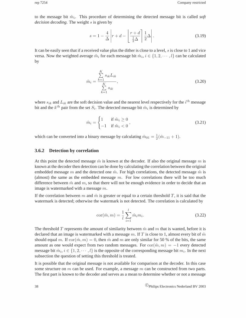
rep 7254 Company restricted
to the message bitmi. This procedure of determining the detected message bit is calledsoftdecision decoding. The weights is given by
s = 1 − 4∆
∣∣∣∣∣r + d −⌊
r + d12∆
⌉12∆
∣∣∣∣∣ . (3.19)
It can be easily seen that if a received value plus the dither is close to a level,s is close to 1 and viceversa. Now the weighted averagemi for each message bitmi, i ∈ {1, 2, · · · , l} can be calculatedby
mi =
K∑k=1
sikLik
K∑k=1
sik
, (3.20)
wheresik andLik are the soft decision value and the nearest level respectively for theith messagebit and thekth pair from the setSi. The detected message bitmi is determined by
mi =
{1 if mi ≥ 0−1 if mi < 0
, (3.21)
which can be converted into a binary message by calculatingm01 = 12(m−11 + 1).
3.6.2 Detection by correlation
At this point the detected messagem is known at the decoder. If also the original messagem isknown at the decoder then detection can be done by calculating the correlation between the originalembedded messagem and the detected onem. For high correlations, the detected messagem is(almost) the same as the embedded messagem. For low correlations there will be too muchdifference betweenm andm, so that there will not be enough evidence in order to decide that animage is watermarked with a messagem.
If the correlation betweenm andm is greater or equal to a certain thresholdT , it is said that thewatermark is detected; otherwise the watermark is not detected. The correlation is calculated by
cor(m, m) =1l
l∑i=1
mimi. (3.22)
The thresholdT represents the amount of similarity betweenm andm that is wanted, before it isdeclared that an image is watermarked with a messagem. If T is close to 1, almost every bit ofmshould equalm. If cor(m, m) = 0, thenm andm are only similar for 50 % of the bits, the sameamount as one would expect from two random messages. Forcor(m, m) = −1 every detectedmessage bitmi, i ∈ {1, 2, · · · , l} is the opposite of the corresponding message bitmi. In the nextsubsection the question of setting this threshold is treated.
It is possible that the original message is not available for comparison at the decoder. In this casesome structure onm can be used. For example, a messagem can be constructed from two parts.The first part is known to the decoder and serves as a mean to determine whether or not a message
38 c©Philips Electronics Nederland BV 2003

Company restricted rep 7254
is embedded. This part can be detected by correlation. The second part is an arbitrary message.If the existence of a message is detected by means of the first part, then the second part is thatmessage.
So, summarizing we have the following. A messagem = m(1)m(2) consisting of two parts isembedded in an image. The decision whether or not the received imager is watermarked is basedon: {
cor(m(1), m(1)) > T r is said to be watermarked
cor(m(1), m(1)) ≤ T r is said to be unwatermarked, (3.23)
wherem(1) is known at the detector. Ifr is said to be watermarked, it is said to be watermarkedwith the messagem(2).
Another possibility is to choose messagesm from a codeC, som = c, c ∈ C. The detector knowsthe codebook corresponding to this code. At the detector a messagem is estimated. Ifm is equalto or close enough to a codewordc ∈ C, thenr is said to be watermarked with messagec.
3.6.3 The threshold setting
The threshold settingdetermines the trade-off between the false positive and the false negativeprobabilities. For a high threshold setting the false positive probability will be low; It is unlikelythat in an unwatermarked image, the detected message will be almost identical to the referencemessagem. The probability that detection on an image watermarked with messagem results ina detected messagem almost identical tom, will be low for high thresholds, even for moderateattacks. For lower threshold settings the false negative probabilities are lower, but the false posi-tives probabilities are higher. The false negative probability is hard to model, so we only look atthe false positive probability in order to determine the threshold.
For an unwatermarked image it is also possible to extract a sequence of -1’s and 1’s. The falsepositive probabilityPfp is now considered to be the probability that a detection will occur, i.e., theprobability that the correlation with the reference messagem is higher than the thresholdT , thatis
Pfp = P
(1l
l∑i=1
nimi ≥ T
)(3.24)
Because the reference messagem usually has an equal amount of -1’s and 1’s, it is assumed thatm is uniformly distributed withP (mi = −1) = p andP (mi = +1) = 1 − p, with p = 1
2 . Weassume that a messagen extracted from an unwatermarked image is also uniformly distributed,with P (mi = −1) = q, P (mi = +1) = 1 − q andq = 1
2 . This assumption is valid, becausethe dither makes the pixel values uniformly distributed over a quantization bin [20, 24, 31], so theprobability that a pixel value is closest to an even or an odd level is equal to1
2 .
In order to derive the probability (3.24), first the distribution ofSl = 1l
l∑i=1
zi, with zi = nimi, has
to be derived. We prove that the distribution ofSl can be approximated by a normal distribution:
Theorem 3.3.
liml→∞
P(√
l Sl ≤ x)
=12
erf(
x√2
), ∀x ∈ R,
c©Philips Electronics Nederland BV 2003 39
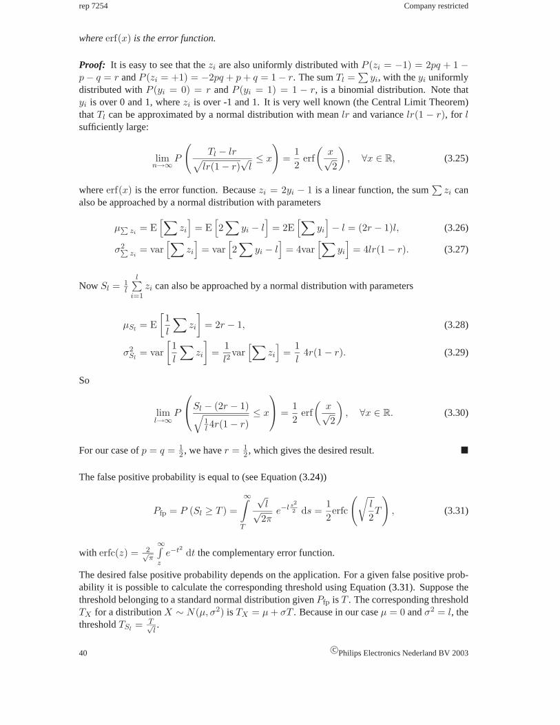
rep 7254 Company restricted
whereerf(x) is the error function.
Proof: It is easy to see that thezi are also uniformly distributed withP (zi = −1) = 2pq + 1 −p − q = r andP (zi = +1) = −2pq + p + q = 1 − r. The sumTl =
∑yi, with theyi uniformly
distributed withP (yi = 0) = r andP (yi = 1) = 1 − r, is a binomial distribution. Note thatyi is over 0 and 1, wherezi is over -1 and 1. It is very well known (the Central Limit Theorem)thatTl can be approximated by a normal distribution with meanlr and variancelr(1 − r), for lsufficiently large:
limn→∞P
(Tl − lr√
lr(1 − r)√
l≤ x
)=
12
erf(
x√2
), ∀x ∈ R, (3.25)
whereerf(x) is the error function. Becausezi = 2yi − 1 is a linear function, the sum∑
zi canalso be approached by a normal distribution with parameters
µ∑zi
= E[∑
zi
]= E
[2∑
yi − l]
= 2E[∑
yi
]− l = (2r − 1)l, (3.26)
σ2∑zi
= var[∑
zi
]= var
[2∑
yi − l]
= 4var[∑
yi
]= 4lr(1 − r). (3.27)
Now Sl = 1l
l∑i=1
zi can also be approached by a normal distribution with parameters
µSl= E
[1l
∑zi
]= 2r − 1, (3.28)
σ2Sl
= var[1l
∑zi
]=
1l2
var[∑
zi
]=
1l
4r(1 − r). (3.29)
So
liml→∞
P
Sl − (2r − 1)√
1l 4r(1 − r)
≤ x
=
12
erf(
x√2
), ∀x ∈ R. (3.30)
For our case ofp = q = 12 , we haver = 1
2 , which gives the desired result. �
The false positive probability is equal to (see Equation (3.24))
Pfp = P (Sl ≥ T ) =
∞∫T
√l√
2πe−l s2
2 ds =12erfc
(√l
2T
), (3.31)
with erfc(z) = 2√π
∞∫z
e−t2 dt the complementary error function.
The desired false positive probability depends on the application. For a given false positive prob-ability it is possible to calculate the corresponding threshold using Equation (3.31). Suppose thethreshold belonging to a standard normal distribution givenPfp is T . The corresponding thresholdTX for a distributionX ∼ N(µ, σ2) is TX = µ + σT . Because in our caseµ = 0 andσ2 = l, thethresholdTSl
= T√l.
40 c©Philips Electronics Nederland BV 2003

Company restricted rep 7254
l T10−3 T exp10−3 T10−5 T exp
10−5 T10−7 T10−15
10 0.977 0.999 1.350 0.999 1.644 2.51050 0.437 0.439 0.604 0.600 0.735 1.123
100 0.309 0.301 0.427 0.419 0.520 0.794500 0.138 0.137 0.191 0.188 0.233 0.355
1000 0.098 0.098 0.135 0.137 0.164 0.251
Table 3.1: Threshold settings for false positive probabilitiesPfp ∈ {10−3, 10−5, 10−7, 10−15}. Tis the theoretical derived threshold andT exp the threshold resulting from experiments.
This thresholdTSlis calculated for the false positive probabilities{10−3, 10−5, 10−7 and10−15}.
ForPfp = 10−3 andPfp = 10−5 this threshold is also determined by experiment in order to verifythe model behind the theoretically calculated thresholds. ForPfp = 10−3, 100.000 messages arepseudo randomly created and their correlation is calculated with an also pseudo randomly createdreference message. Then it is investigated for which threshold settingTSl
the number of falsepositives is smaller than or equal to 100 (a maximum of 100 false positives out of 100.000 givesPfp ≤ 10−3). ForPfp = 10−5 we have taken 10.000.000 sample messages. The results are statedin Table3.1.
For low message lengths (l = 10) the theoretical results do not match with the experimental results.This is because the normal distribution is not a good approximation of the binomial distributionfor low values ofl. For higher values ofl both results correspond, so we conclude that the modelis correct for message lengths of at least 50. For lower message lengthsl, the thresholdT can bedetermined by experiments.
As said before, the threshold setting is a trade-off between the false positive and the false negativeprobability. If the threshold is chosen asT = 1, all bits must be correct, so it is very likely thatan embedded message will not be detected and the false negative probability will be high. If thethreshold is chosen asT = 0, the false positive probability will bePfp = P (Sl ≥ 0) = 1
2 (seeEquation (3.31)), which is very high.
3.7 Summary
We summarize the SCS embedding and detection methods, as they will be used throughout theremainder of this report.
• Embedding a messagem in a host signalx is done by
ySCS = x + α
(⌊x + d − 1
2m∆∆
⌉∆ − x − d +
m∆2
), (3.32)
where the ditherd, the quantization stepsize∆ and the distortion compensation parameterαare determined in advance. The ditherd is a pseudo random uniformly distributed sequenceand serves as a secret key.∆ andα are parameters to control robustness and perceptibility.The watermarked imagey is sent over a channel, which models an attack.
c©Philips Electronics Nederland BV 2003 41
rep 7254 Company restricted
• At the detector the imager is received. The messagem is detected by
m =
⌊r + d12∆
⌉(mod 2). (3.33)
In order to determine whether or not the received imager was watermarked, the correlationwith the reference messagem is calculated by
cor(m, m) =1l
l∑i=1
mimi. (3.34)
For correlations higher than a thresholdT , the image is said to be watermarked with messagem.
42 c©Philips Electronics Nederland BV 2003

Chapter 4
Problem description and Contributions
In Chapter2 a general introduction to watermarking has been given. Because of the possiblehigh payloads, attention has been focussed on the class of quantization watermark systems inChapter3, notably Quantization Index Modulation and the extension Distortion CompensatedQIM, the Costa scheme and the Scalar Costa Scheme. For a Gaussian host signal and an AWGNchannel the DC-QIM or Costa’s scheme are optimal; They achieve the same capacity as non-blinddetection. However, these schemes are not practical. The SCS is practical and sub-optimal underthe condition thatx ∼ N(0, σ2
xIN ) and the noise is AWGN.
In the real world these conditions may not be satisfied. Digital images are usually not Gaussiandistributed and all the various attacks, discussed in Section2.5, cannot be modelled by AWGN.For JPEG compression, for example, the noisen is highly correlated with the host signalx. Forthese reasons it is necessary to adapt the SCS, so that it can also be robust against other attacks,like, JPEG-compression and brightness scaling.
This reports focuses on two possible solutions to these deficiencies. The first solution is the useof Error Correcting Codes (ECC). Instead of embedding a messagem into an image, it is encodedinto the coded messagemc, which in turn is embedded. At the detector an estimate of this encodedmessagemc is retrieved. Using an error correcting decoding mechanism an estimate of the originalmessagem is found, with less errors than in the case of embeddingm directly into the image. Ashort introduction to ECC’s and an experimental evaluation of the performance increase by ECCmethods is presented in Chapter5.
Another solution is the use of an adaptive quantization step size. In standard SCS the quantizationstep size∆ is fixed and known at both the embedder and the detector. An adaptive quantizationstep size is dependent on the host signalx. Adaptive quantization introduces robustness againstthe attack of scaling the brightness values. At the same time it gives a more efficient allocation ofwatermark energy, because this allocation is conform a (simple) Human Visual Model: Weber’slaw, see Section2.4. We will investigate several methods to implement adaptive quantization inChapter6. The performance of the several methods of adaptive quantization is compared with eachother and with fixed quantization. The robustness gain with regard to brightness scaling comparedto the use of a fixed quantization step size is also verified by experiment in this chapter.
We want to have a mathematical analysis of the performance of our adaptive quantization water-marking system. As a measure of performance the bit error probability is taken. This bit errorprobability is build up from two components: one which takes into account AWGN and uniformnoise, with a fixed quantization step size, and the other an adaptive quantization step size, without
43

rep 7254 Company restricted
noise. Stochastic models for these two bit error probabilities are developed in Chapter7.
The performance of the watermarking model depends on some system parameters, like the dis-tortion compensation parameterα. An optimal value of this parameter should be applied at theencoder in order to get optimal performance. This optimization problem is treated in Chapter8;The result is compared with a similar result of Joachim Eggers.
Summarizing, we have
• Improvements of current quantization based watermarking schemes have to be sought, inorder to increase robustness;
• A first improvement is the use of ECC’s. The increase of overall robustness is verified byexperiment;
• A second improvement is the use of an adaptive quantization step size. A gain in robustnessagainst brightness scaling is verified, both analytically and experimentally. The performanceof adaptive quantization is compared with fixed quantization by experiment;
• An analytical performance analysis of the new watermarking system is made;
• The distortion compensation parameterα is optimized for a Gaussian signal and an AWGNchannel.
44 c©Philips Electronics Nederland BV 2003
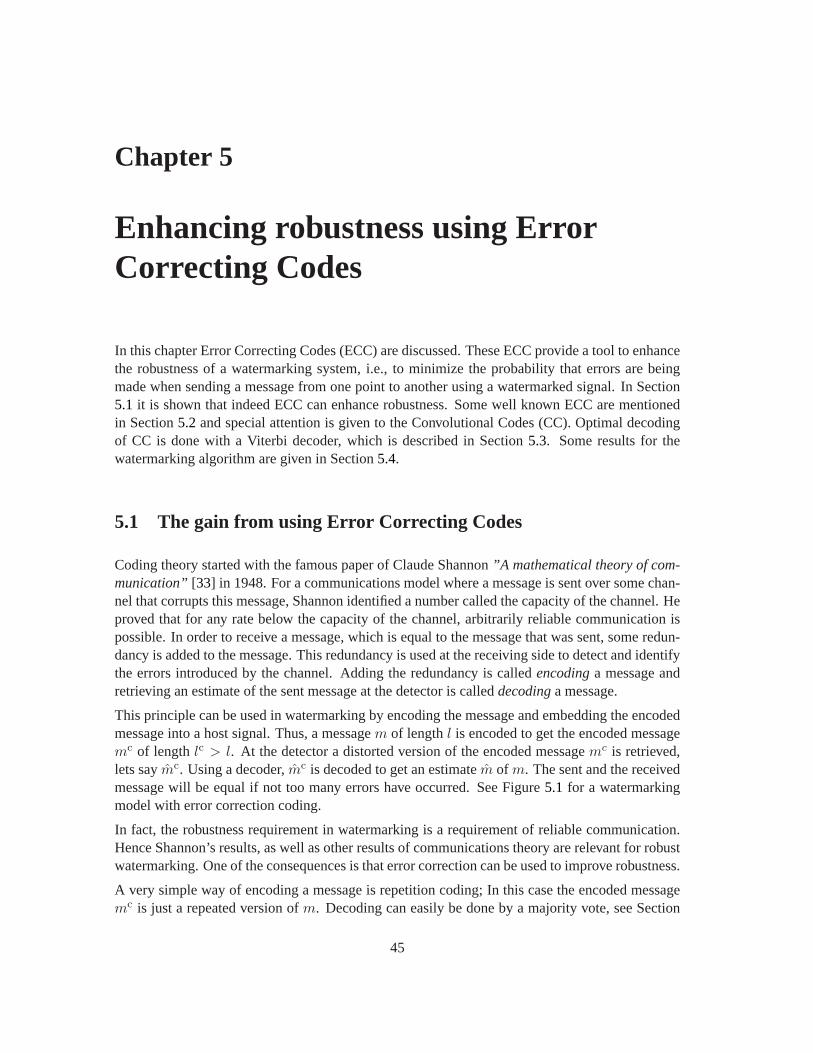
Chapter 5
Enhancing robustness using ErrorCorrecting Codes
In this chapter Error Correcting Codes (ECC) are discussed. These ECC provide a tool to enhancethe robustness of a watermarking system, i.e., to minimize the probability that errors are beingmade when sending a message from one point to another using a watermarked signal. In Section5.1 it is shown that indeed ECC can enhance robustness. Some well known ECC are mentionedin Section5.2 and special attention is given to the Convolutional Codes (CC). Optimal decodingof CC is done with a Viterbi decoder, which is described in Section5.3. Some results for thewatermarking algorithm are given in Section5.4.
5.1 The gain from using Error Correcting Codes
Coding theory started with the famous paper of Claude Shannon”A mathematical theory of com-munication” [33] in 1948. For a communications model where a message is sent over some chan-nel that corrupts this message, Shannon identified a number called the capacity of the channel. Heproved that for any rate below the capacity of the channel, arbitrarily reliable communication ispossible. In order to receive a message, which is equal to the message that was sent, some redun-dancy is added to the message. This redundancy is used at the receiving side to detect and identifythe errors introduced by the channel. Adding the redundancy is calledencodinga message andretrieving an estimate of the sent message at the detector is calleddecodinga message.
This principle can be used in watermarking by encoding the message and embedding the encodedmessage into a host signal. Thus, a messagem of lengthl is encoded to get the encoded messagemc of lengthlc > l. At the detector a distorted version of the encoded messagemc is retrieved,lets saymc. Using a decoder,mc is decoded to get an estimatem of m. The sent and the receivedmessage will be equal if not too many errors have occurred. See Figure5.1 for a watermarkingmodel with error correction coding.
In fact, the robustness requirement in watermarking is a requirement of reliable communication.Hence Shannon’s results, as well as other results of communications theory are relevant for robustwatermarking. One of the consequences is that error correction can be used to improve robustness.
A very simple way of encoding a message is repetition coding; In this case the encoded messagemc is just a repeated version ofm. Decoding can easily be done by a majority vote, see Section
45
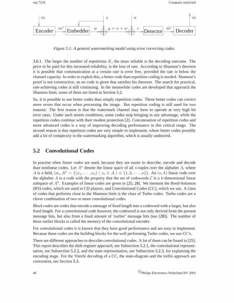
rep 7254 Company restricted
Encoder Embedder Detector Decoder
m
y = x + w
m
mc w r
x n
mc
Figure 5.1: A general watermarking model using error correcting codes.
3.6.1. The larger the number of repetitionsK, the more reliable is the decoding outcome. Theprice to be paid for this increased reliability, is the loss of rate. According to Shannon’s theoremit is possible that communication at a certain rate is error free, provided the rate is below thechannel capacity. In order to exploit this, a better code than repetition coding is needed. Shannon’sproof is not constructive, so no code is given that satisfies his theorem. The search for practical,rate-achieving codes is still continuing. In the meanwhile codes are developed that approach theShannon limit, some of them are listed in Section5.2.
So, it is possible to use better codes than simply repetition codes. These better codes can correctmore errors that occur when processing the image. But repetition coding is still used for tworeasons: The first reason is that the watermark channel may have to operate at very high biterror rates. Under such severe conditions, some codes stop bringing in any advantage, while therepetition codes continue with their modest protection [2]. Concatenation of repetition codes andmore advanced codes is a way of improving decoding performance in this critical range. Thesecond reason is that repetition codes are very simple to implement, where better codes possiblyadd a lot of complexity to the watermarking algorithm, which is usually undesired.
5.2 Convolutional Codes
In practise oftenlinear codesare used, because they are easier to describe, encode and decodethan nonlinear codes. LetAn denote the linear space of alln-tuples over the alphabetA, whereA is a field, i.e.,An = {(x1, · · · , xn) | xi ∈ A, i ∈ {1, 2, · · · , n}}. An (n, k) linear code overthe alphabetA is a code with the property that the set of codewordsC is ak-dimensional linearsubspace ofAn. Examples of linear codes are given in [25, 28]. We mention the Reed-Solomon(RS) codes, which are used in CD players, and Convolutional Codes (CC), which we use. A classof codes that performs close to the Shannon limit is the class of Turbo codes. Turbo codes are aclever combination of two or more convolutional codes.
Block codesare codes that encode a message of fixed length into a codeword with a larger, but alsofixed length. For aconvolutional codehowever, the codeword is not only derived from the presentmessage bits, but also from a fixed amount of ’earlier’ message bits (see [28]). The number ofthese earlier blocks is called thememoryof the convolutional encoder.
For convolutional codes it is known that they have good performance and are easy to implement.Because these codes are the building blocks for the well performing Turbo codes, we use CC’s.
There are different approaches to describe convolutional codes. A lot of them can be found in [25].This report describes the shift-register approach, see Subsection5.2.1, the convolutional represen-tation, see Subsection5.2.2, and the state representation, see Subsection5.2.3, for explaining theencoding stage. For the Viterbi decoding of a CC, the state-diagram and the trellis approach areconvenient, see Section5.3.
46 c©Philips Electronics Nederland BV 2003
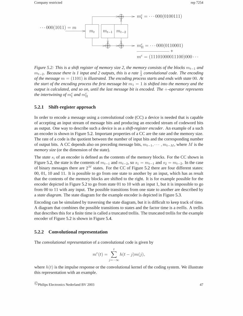
Company restricted rep 7254
mc = (11101000011100)000 · · ·
mt
· · · 000(1011) = mmt−1 mt−2
mcI = · · · 000(0100111)
mcII = · · · 000(0110001)
+
Figure 5.2: This is a shift register of memory size 2, the memory consists of the blocksmt−1 andmt−2. Because there is 1 input and 2 outputs, this is a rate1
2 convolutional code. The encodingof the messagem = (1101) is illustrated. The encoding process starts and ends with state00. Atthe start of the encoding process the first message bitm1 = 1 is shifted into the memory and theoutput is calculated, and so on, until the last message bit is encoded. The+-operator representsthe intertwining ofmc
I andmcII
5.2.1 Shift-register approach
In order to encode a message using a convolutional code (CC) a device is needed that is capableof accepting an input stream of message bits and producing an encoded stream of codeword bitsas output. One way to describe such a device is as ashift-register encoder. An example of a suchan encoder is shown in Figure5.2. Important properties of a CC are the rate and the memory size.The rate of a code is the quotient between the number of input bits and the corresponding numberof output bits. A CC depends also on preceding message bits,mt−1, · · · , mt−M , whereM is thememory size(or the dimension of the state).
Thestatesi of an encoder is defined as the contents of the memory blocks. For the CC shown inFigure5.2, the state is the contents ofmt−1 andmt−2, sos1 = mt−1 ands2 = mt−2. In the caseof binary messages there are2M states. For the CC of Figure5.2 there are four different states:00, 01, 10 and 11. It is possible to go from one state to another by an input, which has as resultthat the contents of the memory blocks are shifted to the right. It is for example possible for theencoder depicted in Figure5.2 to go from state 01 to 10 with an input 1, but it is impossible to gofrom 00 to 11 with any input. The possible transitions from one state to another are described byastate diagram. The state diagram for the example encoder is depicted in Figure5.3.
Encoding can be simulated by traversing the state diagram, but it is difficult to keep track of time.A diagram that combines the possible transitions to states and the factor time is atrellis. A trellisthat describes this for a finite time is called a truncated trellis. The truncated trellis for the exampleencoder of Figure5.2 is shown in Figure5.4.
5.2.2 Convolutional representation
Theconvolutional representationof a convolutional code is given by
mc(t) =t∑
j=−∞h(t − j)m(j),
whereh(t) is the impulse response or the convolutional kernel of the coding system. We illustratethis representation with an example.
c©Philips Electronics Nederland BV 2003 47
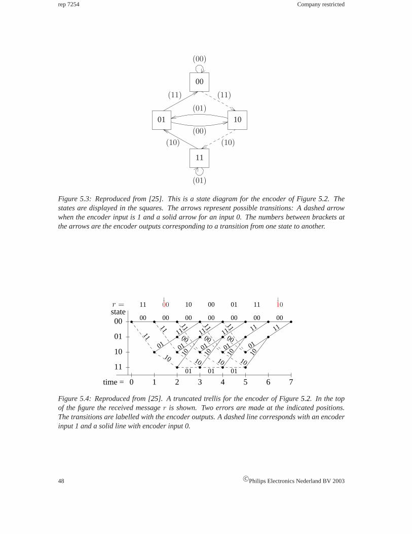
rep 7254 Company restricted
(00)
01
00
10
11
(10)
(01)
(01)
(00)
(10)
(11)(11)
Figure 5.3: Reproduced from [25]. This is a state diagram for the encoder of Figure5.2. Thestates are displayed in the squares. The arrows represent possible transitions: A dashed arrowwhen the encoder input is 1 and a solid arrow for an input 0. The numbers between brackets atthe arrows are the encoder outputs corresponding to a transition from one state to another.
00 00
11
10
00 00 00 00 00
11
11 11 11
01 0101 0101
10 101001 01 01
10 10 10 10
11 11 11 1111
00 0000
11 10 00 01 11
0 1 2 3 4 5 76time =
state
01
10
11
00
r =↓00
↓10
Figure 5.4: Reproduced from [25]. A truncated trellis for the encoder of Figure5.2. In the topof the figure the received messager is shown. Two errors are made at the indicated positions.The transitions are labelled with the encoder outputs. A dashed line corresponds with an encoderinput 1 and a solid line with encoder input 0.
48 c©Philips Electronics Nederland BV 2003
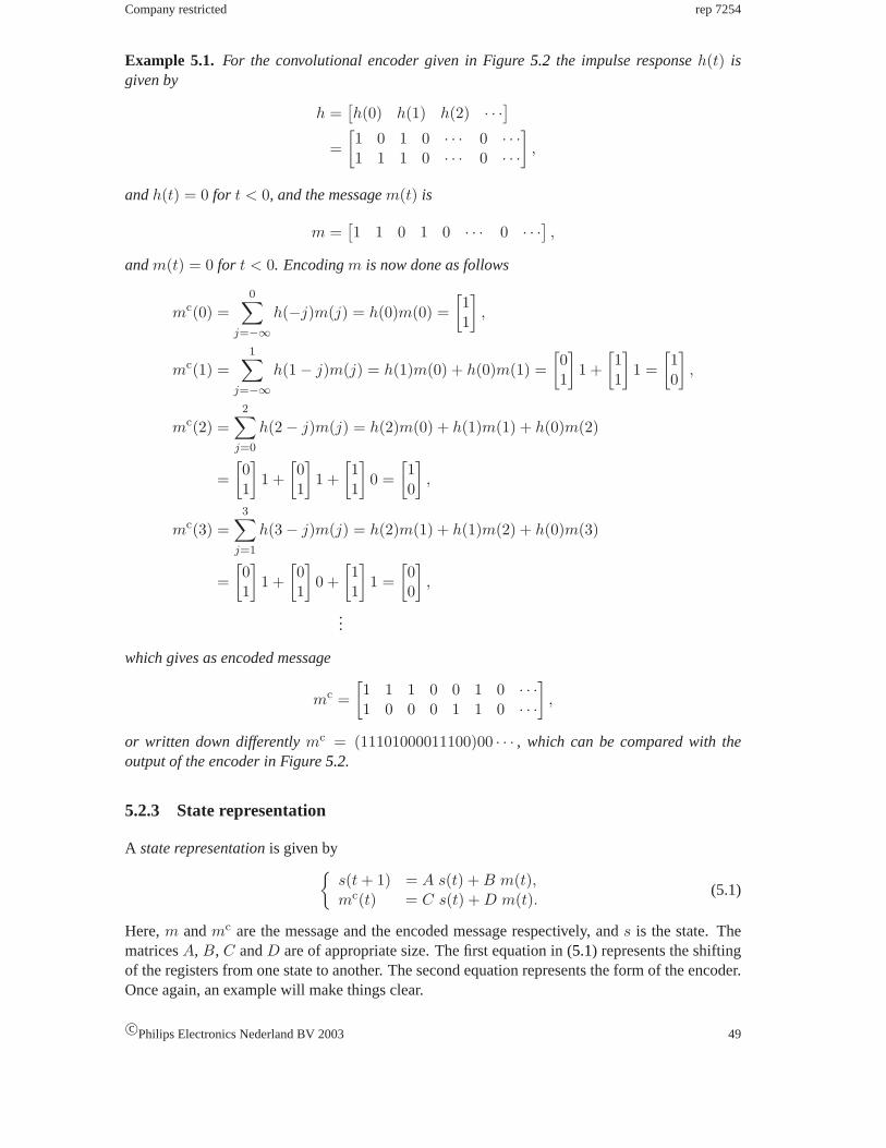
Company restricted rep 7254
Example 5.1. For the convolutional encoder given in Figure5.2 the impulse responseh(t) isgiven by
h =[h(0) h(1) h(2) · · ·]
=[1 0 1 0 · · · 0 · · ·1 1 1 0 · · · 0 · · ·
],
andh(t) = 0 for t < 0, and the messagem(t) is
m =[1 1 0 1 0 · · · 0 · · ·] ,
andm(t) = 0 for t < 0. Encodingm is now done as follows
mc(0) =0∑
j=−∞h(−j)m(j) = h(0)m(0) =
[11
],
mc(1) =1∑
j=−∞h(1 − j)m(j) = h(1)m(0) + h(0)m(1) =
[01
]1 +
[11
]1 =
[10
],
mc(2) =2∑
j=0
h(2 − j)m(j) = h(2)m(0) + h(1)m(1) + h(0)m(2)
=[01
]1 +
[01
]1 +
[11
]0 =
[10
],
mc(3) =3∑
j=1
h(3 − j)m(j) = h(2)m(1) + h(1)m(2) + h(0)m(3)
=[01
]1 +
[01
]0 +
[11
]1 =
[00
],
...
which gives as encoded message
mc =[1 1 1 0 0 1 0 · · ·1 0 0 0 1 1 0 · · ·
],
or written down differentlymc = (11101000011100)00 · · · , which can be compared with theoutput of the encoder in Figure5.2.
5.2.3 State representation
A state representationis given by{s(t + 1) = A s(t) + B m(t),mc(t) = C s(t) + D m(t).
(5.1)
Here,m andmc are the message and the encoded message respectively, ands is the state. ThematricesA, B, C andD are of appropriate size. The first equation in (5.1) represents the shiftingof the registers from one state to another. The second equation represents the form of the encoder.Once again, an example will make things clear.
c©Philips Electronics Nederland BV 2003 49

rep 7254 Company restricted
Example 5.2. For the convolutional encoder given in Figure5.2 the state representation is givenby
s(t + 1) =[0 01 0
]s(t) +
[10
]m(t),
mc(t) =[0 11 1
]s(t) +
[11
]m(t).
s(0) = 0
(5.2)
The coding of a messagem = (1101)00 · · · is done as follows
t = 0 =⇒ s(1) =[10
], mc(0) =
[11
]
t = 1 =⇒ s(2) =[11
], mc(1) =
[10
]
t = 2 =⇒ s(3) =[01
], mc(2) =
[10
]...
This gives as encoded messagemc = (11101000011100)00 · · · . Compare this with Figure5.2and Example5.1.
5.3 Viterbi decoder
Convolutional codes can be decoded with a number of decoding algorithms, one of which is Viterbidecoding. When a decoder receives a sequence, it has to estimate the sequence that was reallysent. The decoder will be optimal if it chooses the estimate that maximizes some log-likelihoodfunction. Viterbi decoding is convenient in the sense that it is maximum likelihood [23], but thecomplexity is an exponential function of the memory depthM .
The trellis representation of the encoding process, see Figure5.4, can be used to decode a CC. Butit is needed to label the edges of the trellis with some distance measure. This distance measureis for hard decision decoding often the Hamming distance, and for soft decision decoding theEuclidean distance. In Figure5.5 the trellis is shown, with edges labelled with the Hammingdistance between the received encoded message bits and the possible encoder outputs. The totalHamming distance between the received encoded messager and a codewordc is the sum of alllabels on the path corresponding to that codeword. This sum is just the length of the trellis pathcorresponding to that codeword.
Decoding the received messager is a matter of finding the codeword closest tor. This is equivalentto finding the shortest path from the start to the end of the trellis. Finding the shortest path can bedone using the Viterbi algorithm. TheViterbi algorithmis a form of dynamic programming. It isbased upon the simple observation that once the shortest paths to all states at timet is found, theshortest paths at timet + 1 can be constructed from the former paths. The Viterbi algorithm isillustrated by decoding a received encoded message for the example CC, as shown in Figure5.6.
More formally, the Viterbi decoding algorithm is given by the following scheme. The time isdenoted byt. The states are in the setS, and the all-zero state is denoted by0. The labels of the
50 c©Philips Electronics Nederland BV 2003
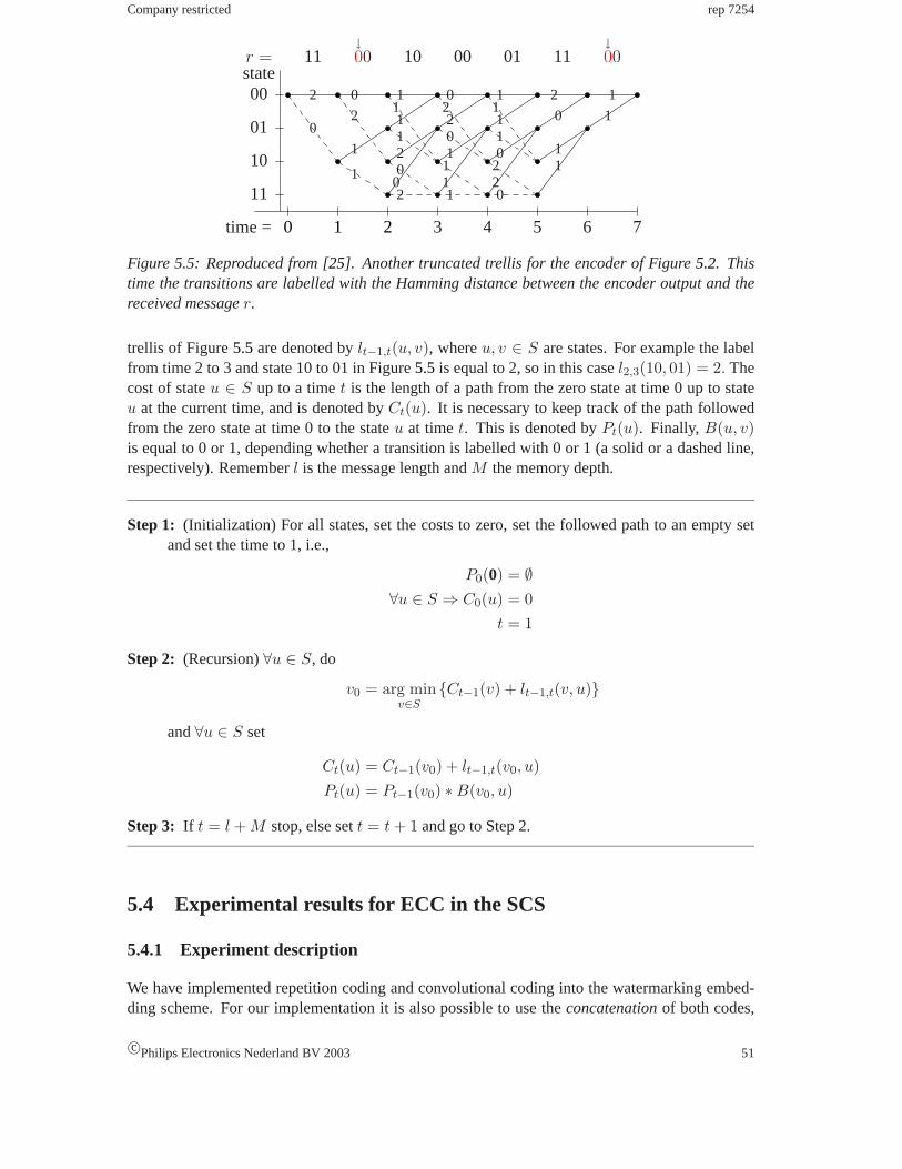
Company restricted rep 7254
0 1 2
↓00
3 4 5 76time =
state
01
10
11
00 2
0
0
2
1
2
0211
11
0
1
02201
111
11110
0
22
2
0
11
1
1
11r = 10 110100↓00
Figure 5.5: Reproduced from [25]. Another truncated trellis for the encoder of Figure5.2. Thistime the transitions are labelled with the Hamming distance between the encoder output and thereceived messager.
trellis of Figure5.5 are denoted bylt−1,t(u, v), whereu, v ∈ S are states. For example the labelfrom time 2 to 3 and state 10 to 01 in Figure5.5is equal to 2, so in this casel2,3(10, 01) = 2. Thecost of stateu ∈ S up to a timet is the length of a path from the zero state at time 0 up to stateu at the current time, and is denoted byCt(u). It is necessary to keep track of the path followedfrom the zero state at time 0 to the stateu at timet. This is denoted byPt(u). Finally, B(u, v)is equal to 0 or 1, depending whether a transition is labelled with 0 or 1 (a solid or a dashed line,respectively). Rememberl is the message length andM the memory depth.
Step 1: (Initialization) For all states, set the costs to zero, set the followed path to an empty setand set the time to 1, i.e.,
P0(0) = ∅∀u ∈ S ⇒ C0(u) = 0
t = 1
Step 2: (Recursion)∀u ∈ S, do
v0 = arg minv∈S
{Ct−1(v) + lt−1,t(v, u)}
and∀u ∈ S set
Ct(u) = Ct−1(v0) + lt−1,t(v0, u)Pt(u) = Pt−1(v0) ∗ B(v0, u)
Step 3: If t = l + M stop, else sett = t + 1 and go to Step 2.
5.4 Experimental results for ECC in the SCS
5.4.1 Experiment description
We have implemented repetition coding and convolutional coding into the watermarking embed-ding scheme. For our implementation it is also possible to use theconcatenationof both codes,
c©Philips Electronics Nederland BV 2003 51

rep 7254 Company restricted
Cost2
1
4
1
01
10
11
00
0 1
state
20 1
state
01
10
11
00Cost
2
−
0
−
Step 1 Step 2
01
10
11
00
0 1
state
2 3
Cost2
1
2
3
Step 3
01
10
11
00
0 1
state
2 3
Cost2
3
1
3
4
Step 4
01
10
11
00
0 1
state
2 3 4 5 6
Cost1
4
−
−
Step 6
01
10
11
00
0 1
state
2 3 4 5
Cost3
1
3
3
Step 5
01
10
11
00
0 1
state
2 3 4 5 6 7
Cost2
−
−
−
Step 7
t =
t =
t =t =
t =
t = t =
Figure 5.6: The Viterbi algorithm. For each state and each time, the shortest path and the cor-responding costs are calculated using the Viterbi algorithm. For each step the shortest path isdepicted in green. The decoded message can easily be read off, by following the shortest path (ingreen), and is found to bem = (1101).
52 c©Philips Electronics Nederland BV 2003

Company restricted rep 7254
CCencoder
repetitionencoder
Embedder
CCdecoder(Viterbi)
repetitiondecoder
Detector
n
mc2 wm mc1
x
y = x + w
m mc1 mc2 r
Figure 5.7: A watermarking model using concatenated codes.
with the convolutional code as an outer code. This means that the massagem is first encoded usingconvolutional coding, resulting inmc1 with lengthlc1 , and thanmc1 is encoded using a repetitioncode, resulting inmc2 , with lengthlc2 , where usuallylc2 = N . See Figure5.7for illustration.
It is possible for our implementation to use an arbitrary number of inputsk and outputsn, so anyrate k
n can be achieved. In the detector a Viterbi decoder is used. The Viterbi algorithm uses morecomputer memory if a larger CC memory sizeM is used; This relation is exponential. There is alinear relationship between the message lengthl and the decoding time. For our implementationit is possible on a PIV 1.7 GHz with 256 MB internal memory, to use a CC memory sizeM uptill 9. We observed that the complexity of a watermarking algorithm with convolutional coding ismuch larger than one without, because decoding time increases dramatically.
In order to be able to determine the performance of the watermarking algorithm, we have carriedout some experiments. Testing was done using repetition coding or a concatenated code (CC andrepetition coding together), for different rates, different watermark strengths and different attackswith different strengths. We performed two kinds of attacks: namely AWGN and JPEG attacks.We varied the watermark varianceσ2
w, the noise varianceσ2n of the AWGN and the quality factor
of the JPEG compression. In order to be able to know the relative strength of the watermarkcompared to the host signal, theDocument-to-Watermark Ratio(DWR) is used:
DWR = 10 log10
(σ2
x
σ2w
), (5.3)
where the document is in fact the host signal. In our experiments we have used the NASA CC,depicted in Figure5.8, because it is known that this code has a large minimum distance.
We have done experiments on four images, namelylena.bmp, baboon.bmp, peppers.bmpandtulips.bmp, see AppendixB. Because the experiments are limited only qualitative con-clusions can be drawn, not quantitative.
5.4.2 Results and discussion
The results of these experiments are displayed in Figure5.9 - 5.13. The Bit Error Rates (BER’s)in the graphs are the average BER’s for the four images used for the experiments.
Some qualitative conclusions can be drawn from these figures. We see that outcome of the exper-iments is in line with what we would expect. In Figure5.9 it is seen that if the AWGN varianceσ2
n increases, also the BER increases. In Figure5.10we see that the BER decreases if the JPEG
c©Philips Electronics Nederland BV 2003 53
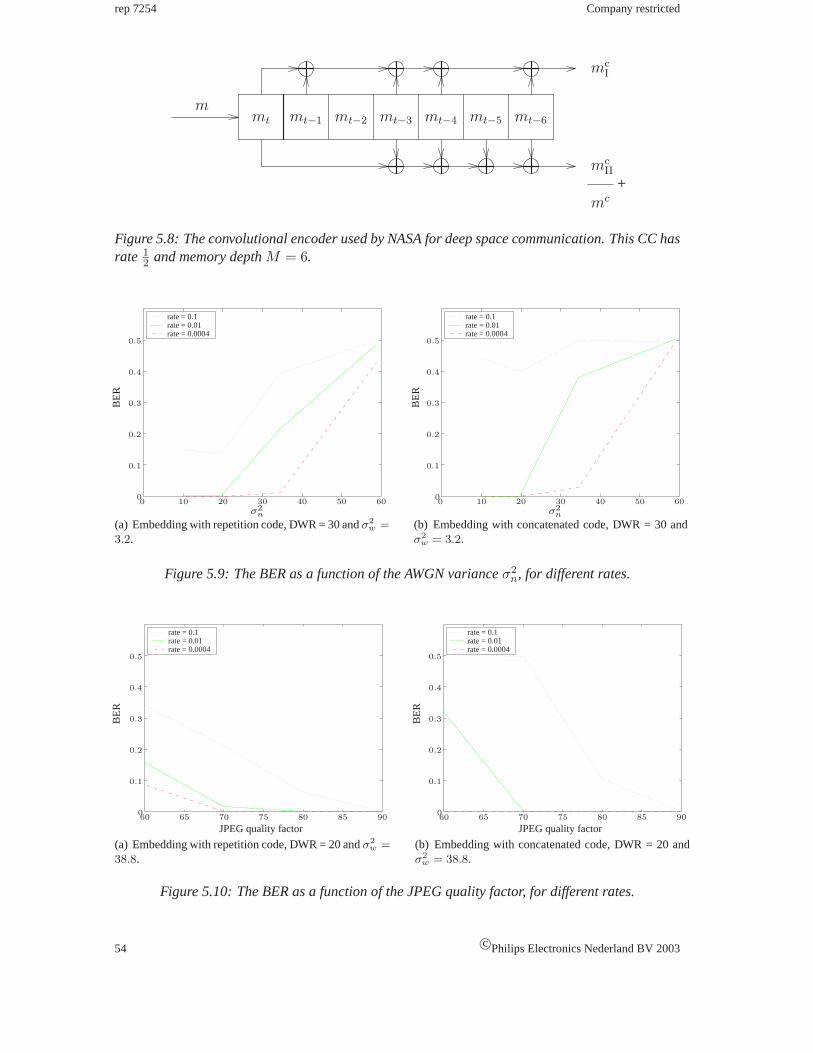
rep 7254 Company restricted
+
mt−2mt−1mt
mmt−3 mt−4 mt−5 mt−6
mcI
mcII
mc
Figure 5.8: The convolutional encoder used by NASA for deep space communication. This CC hasrate 1
2 and memory depthM = 6.
rate = 0.1rate = 0.01rate = 0.0004
BE
R
σ2n
00
0.1
0.2
0.3
0.4
0.5
10 20 30 40 50 60
(a) Embedding with repetition code, DWR = 30 andσ2w =
3.2.
rate = 0.1rate = 0.01rate = 0.0004
BE
R
σ2n
00
0.1
0.2
0.3
0.4
0.5
10 20 30 40 50 60
(b) Embedding with concatenated code, DWR = 30 andσ2
w = 3.2.
Figure 5.9: The BER as a function of the AWGN varianceσ2n, for different rates.
rate = 0.1rate = 0.01rate = 0.0004
BE
R
JPEG quality factor
0
0.1
0.2
0.3
0.4
0.5
60 65 70 75 80 85 90
(a) Embedding with repetition code, DWR = 20 andσ2w =
38.8.
rate = 0.1rate = 0.01rate = 0.0004
BE
R
JPEG quality factor
0
0.1
0.2
0.3
0.4
0.5
60 65 70 75 80 85 90
(b) Embedding with concatenated code, DWR = 20 andσ2
w = 38.8.
Figure 5.10: The BER as a function of the JPEG quality factor, for different rates.
54 c©Philips Electronics Nederland BV 2003

Company restricted rep 7254
rate = 0.1rate = 0.01rate = 0.0004
BE
R
DWR
0
0.1
0.2
0.3
0.4
0.5
20 21 22 23 24 25 26 27 28 29 30
(a) Embedding with repetition code, an AWGN attackwith σ2
n = 58.8.
rate = 0.1rate = 0.01rate = 0.0004
BE
RDWR
0
0.1
0.2
0.3
0.4
0.5
20 21 22 23 24 25 26 27 28 29 30
(b) Embedding with repetition code, a jpeg attack withquality factor 90 andσ2
n = 42.0.
rate = 0.1rate = 0.01rate = 0.0004
BE
R
DWR0
0.1
0.2
0.3
0.4
0.5
20 21 22 23 24 25 26 27 28 29 30
(c) Embedding with concatenated code, an AWGN attackwith σ2
n = 58.8.
rate = 0.1rate = 0.01rate = 0.0004
BE
R
DWR0
0.1
0.2
0.3
0.4
0.5
20 21 22 23 24 25 26 27 28 29 30
(d) Embedding with concatenated code, a jpeg attack withquality factor 90 andσ2
n = 42.0.
Figure 5.11: The BER as a function of the DWR, for different rates.
c©Philips Electronics Nederland BV 2003 55

rep 7254 Company restricted
DWR = 30DWR = 25DWR = 20
BE
R
rate
00
0.06
0.08
0.12
0.14
0.16
0.18
0.01
0.02
0.02 0.03
0.04
0.04 0.05
0.10
0.20
(a) Embedding with repetition code, a noise attack withσ2
n = 10.0.
DWR = 30DWR = 25DWR = 20
BE
Rrate
00
0.06
0.08
0.12
0.14
0.16
0.18
0.01
0.02
0.02 0.03
0.04
0.04 0.05
0.10
0.20
(b) Embedding with concatenated code, a noise attack withσ2
n = 10.0.
DWR = 30DWR = 25DWR = 20
BE
R
rate0
0.3
0.4
0.5
0.01 0.02 0.03 0.04 0.050.1
0.2
(c) Embedding with repetition code, a jpeg attack withquality factor 90 andσ2
n = 41.0.
DWR = 30DWR = 25DWR = 20
BE
R
rate0
0.3
0.4
0.5
0.01 0.02 0.03 0.04 0.050.1
0.2
(d) Embedding with concatenated code, a jpeg attack withquality factor 90 andσ2
n = 41.0.
Figure 5.12: The BER as a function of the rate, for different DWR’s.
56 c©Philips Electronics Nederland BV 2003

Company restricted rep 7254
BE
R
rate
repetition codingconcatenated coding
0
0.1
0.2
0.3
0.4
0.5
0.01 0.02 0.03 0.04 0.05
(a) The BER versus the rate, for DWR = 30,σ2w = and
σ2n = 10.0.
BE
R
repetition codingconvolutional coding
σ2n
0
0.1
0.2
0.3
0.4
0.5
2 4 6 8 10 12 14 16 18 20
(b) The BER versus the AWGN varianceσ2n, for DWR =
25,σ2w = and rate =1
2.
Figure 5.13: Repetition coding compared with concatenated / convolutional coding.
quality factor increases. In Figure5.11we see that if the DWR increases, also the BER increases.In all these three figures and in Figure5.12we see that if the rate decreases, the BER decreases.All these observations are what one would expect in a watermark environment. Summarizing, wehave
• σ2n ↑ =⇒ BER↑
• JPEG quality factor↑ =⇒ BER↓• DWR ↑ =⇒ BER↑• rate↑ =⇒ BER↑
In Figure5.13(a)repetition coding is compared with concatenated coding and in Figure5.13(b)with convolutional coding. In Figure5.13(a)we see that it is better to use concatenated codingthan repetition coding alone up till a certain rate. In Figure5.13(b)we observe that convolutionalcoding is better than repetition coding up till a certain noise attack strength. For higher AWGNvariances the convolutional code stops bringing in advantage, because to many bits are erroneous.The repetition code continues bringing his modest protection in this noise variance range. Thisalso explains why the concatenated code is doing worse than repetition coding alone if the rate istoo high. The inner repetition code does not bring the bit error low enough if rates are too high,and therefore the convolutional code does not work anymore. See also [2] and Section5.1.
c©Philips Electronics Nederland BV 2003 57

rep 7254 Company restricted
58 c©Philips Electronics Nederland BV 2003
Chapter 6
Enhancing robustness using an adaptivequantization step size
The Scalar Costa Scheme uses a fixed quantization step size∆, i.e., for each pixel of an imagethe same∆ is used. The quantization step size is a parameter to control the tradeoff betweenrobustness and visibility. This is true because a large∆ separates two quantization levels by a largedistance, so a stronger noise signal is needed in order to get an error. On the other hand, for a larger∆ the perceptual distortion is also larger. From Section2.4 it is known that larger modificationscan be made in bright areas of a signal (brightness sensitivity). Therefore robustness can be gainedin those areas by embedding with a larger step size, without losing on the perceptibility aspect.
The most important reason of using anadaptive quantizationstep size is that is gives robustnessagainst brightness changes. This is explained in Section6.1. Another effect of adaptive quanti-zation is that choosing a larger quantization step size in bright areas and a smaller one in darkerregions, is less visible for the human eye.
Some of the advantages and disadvantages are described in Section6.1. In Section6.2options fordetermining the adaptive quantization step size are given and reflected on.
6.1 Advantages and disadvantages
6.1.1 Advantages
There are two advantages when using an adaptive quantization step size. The first one is robust-ness againstbrightness scaling. The second one is that the embedding strength is more or lessproportional to the perceptual sensitivity to distortions.
Because for bright image areas a larger quantization step size is chosen, a larger robustness isachieved in those areas; Information embedded in bright areas can be retrieved at the detectorwith larger reliability. The overall robustness will gain from this adaptive quantization, while thewatermark is as perceptible as in the case of a fixed quantization step size.
Suppose a simple model for determining the adaptive quantization step size is used: there is simplya linear relation between∆ and the group of pixel valuesxi. Such a linear relationship can bedefended by referring to Weber’s law, that gives a linear relationship between the sensitivity of the
59

rep 7254 Company restricted
human eye and the luminance value. So, the quantization step size is determined by
∆(x) =γ
L
L∑i=1
xi, (6.1)
whereL is the number of pixels in the aforementioned group and whereγ is some embeddingstrength parameter. It can easily be seen that this model is brightness scale invariant. If thebrightness of an image is scaled by a factorβ, then in fact the scaled image isxscaled = βx. In theunscaled case, detection is done with the quantization stepsize (6.1) and by calculating
m =⌊
x
∆(x)
⌉mod 2 =
⌊x
γL
∑Li=1 xi
⌉mod 2. (6.2)
In the scaled case detection is done with quantization step size
∆scaled(x) =γ
L
L∑i=1
βxi, (6.3)
and the detection is
m =⌊
xscaled
∆scaled(x)
⌉mod 2 =
⌊βx
γL
∑Li=1 βxi
⌉mod 2, (6.4)
which is equal to the detection in the unscaled case.
6.1.2 Disadvantages
For a fixed quantization step size, both at the embedder and the detector,∆ is known. For anadaptive quantization step size∆ is a function ofx. At the embedder the quantization step size iscalculated by∆(x), but at the detector∆ has to be calculated from the received signalr, so thequantization step size is∆(r) = ∆(y+n). This∆(r) is only an estimation of the quantization stepsize used at the embedder and therefore may not be completely accurate. Because the detectiondepends on the adaptive quantization step size, see Equation (3.18), the estimation error causes biterrors in estimating the received message.
6.2 The adaptation rule
Consider the case without dither modulation and distortion compensation. Conceptually, we wouldlike the quantization step size to be a linear function of the corresponding pixel value, so∆(x) =γx. Then, at the embedder QIM is done by (see Equation (3.14)):
yQIM =
⌊x − 1
2mγx
γx
⌉γx +
mγx
2=
(⌊1γ− m
2
⌉γ +
mγ
2
)x. (6.5)
In this wayyQIM does not contain information about the embedded message bit. This can be seenby applying the detector. In order to estimate the message bit at the detector (see Equation (3.18)),the corresponding quantization step size∆ has to be estimated with∆ = γr. The message bit is
60 c©Philips Electronics Nederland BV 2003
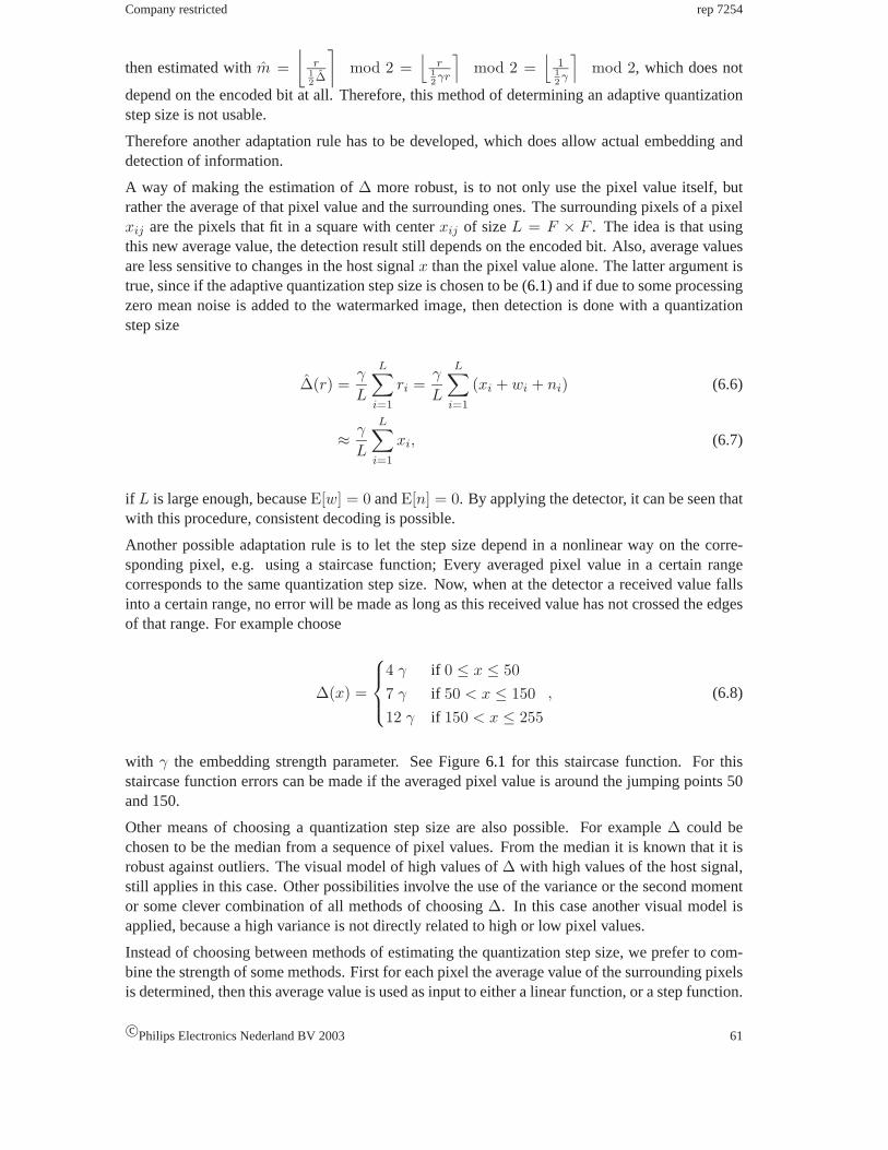
Company restricted rep 7254
then estimated withm =⌊
r12∆
⌉mod 2 =
⌊r
12γr
⌉mod 2 =
⌊112γ
⌉mod 2, which does not
depend on the encoded bit at all. Therefore, this method of determining an adaptive quantizationstep size is not usable.
Therefore another adaptation rule has to be developed, which does allow actual embedding anddetection of information.
A way of making the estimation of∆ more robust, is to not only use the pixel value itself, butrather the average of that pixel value and the surrounding ones. The surrounding pixels of a pixelxij are the pixels that fit in a square with centerxij of sizeL = F × F . The idea is that usingthis new average value, the detection result still depends on the encoded bit. Also, average valuesare less sensitive to changes in the host signalx than the pixel value alone. The latter argument istrue, since if the adaptive quantization step size is chosen to be (6.1) and if due to some processingzero mean noise is added to the watermarked image, then detection is done with a quantizationstep size
∆(r) =γ
L
L∑i=1
ri =γ
L
L∑i=1
(xi + wi + ni) (6.6)
≈ γ
L
L∑i=1
xi, (6.7)
if L is large enough, becauseE[w] = 0 andE[n] = 0. By applying the detector, it can be seen thatwith this procedure, consistent decoding is possible.
Another possible adaptation rule is to let the step size depend in a nonlinear way on the corre-sponding pixel, e.g. using a staircase function; Every averaged pixel value in a certain rangecorresponds to the same quantization step size. Now, when at the detector a received value fallsinto a certain range, no error will be made as long as this received value has not crossed the edgesof that range. For example choose
∆(x) =
4 γ if 0 ≤ x ≤ 507 γ if 50 < x ≤ 15012 γ if 150 < x ≤ 255
, (6.8)
with γ the embedding strength parameter. See Figure6.1 for this staircase function. For thisstaircase function errors can be made if the averaged pixel value is around the jumping points 50and 150.
Other means of choosing a quantization step size are also possible. For example∆ could bechosen to be the median from a sequence of pixel values. From the median it is known that it isrobust against outliers. The visual model of high values of∆ with high values of the host signal,still applies in this case. Other possibilities involve the use of the variance or the second momentor some clever combination of all methods of choosing∆. In this case another visual model isapplied, because a high variance is not directly related to high or low pixel values.
Instead of choosing between methods of estimating the quantization step size, we prefer to com-bine the strength of some methods. First for each pixel the average value of the surrounding pixelsis determined, then this average value is used as input to either a linear function, or a step function.
c©Philips Electronics Nederland BV 2003 61

rep 7254 Company restricted
pixel value
2
4
6
8
10
12
14
00 50 100 150 200 250
∆
Figure 6.1: An example of a staircase function used to determine the adaptive quantization stepsize for a pixel.
So, we use two possibilities for determining the quantization step size:
∆(x) =γ
L
L∑i=1
xi, (6.9)
and
∆(x) = f
(1L
L∑i=1
xi
), (6.10)
with f(·) a staircase function, for example the staircase function of Figure6.1. This staircasefunction is arbitrarily chosen. According to some experiments, it outperforms some other staircasefunctions we have looked at, but it is not claimed that this is the best staircase function. Methodsthat include the usage of a median, the variance or other higher moments are not considered in thisreport.
In order to illustrate the use of an adaptive quantization step size we give an example.
Example 6.1. Let∆(x) be given by (6.9), with L = 9 andγ = 0.05. Let part of the host signalxbe given by
x =
......
......
...· · · 185 188 187 190 191 · · ·· · · 183 170 170 172 180 · · ·· · · 180 165 181 200 205 · · ·· · · 175 179 185 198 206 · · ·· · · 150 190 187 194 201 · · ·
......
......
...
Suppose we want to determine∆ for the pixel in the middle, with value181. The pixels we haveto take into account are the9 pixels that are in the3 × 3 square with centerx = 181. This gives
∆ =0.059
(170 + 170 + 172 + 165 + 181 + 200 + 179 + 185 + 198) = 9.
62 c©Philips Electronics Nederland BV 2003

Company restricted rep 7254
If ∆ was to be determined with (6.10) and staircase function given by (6.8), then we would have
∆ = f
(19
(170 + 170 + 172 + 165 + 181 + 200 + 179 + 185 + 198))
= f (180) = 12.
6.3 Experimental results for an adaptive quantization step size
The robustness properties for both methods are determined by experiment and compared in thissection. In Section7.3we will take a more theoretical look at this robustness.
6.3.1 Experiment description
We perform experiments in order to compare three adaptive quantization methods. We also com-pare the best of the three methods with fixed quantization. We want to evaluate the robustness offixed and adaptive quantization against brightness scaling and AWGN and JPEG attacks.
Adaptive quantization is done by taking an average value over a square of sizeF × F = L, anduse that as an input to either one of the two staircase functions or a linear function. So,we considerthe following three adaptive quantization methods:
Method 1 ∆(x) = f
(1L
L∑i=1
xi
), with
∆(x) =
3 γ if 0 ≤ x ≤ 505 γ if 50 < x ≤ 1008 γ if 100 < x ≤ 15010 γ if 150 < x ≤ 255
. (6.11)
Method 2 ∆(x) = f
(1L
L∑i=1
xi
), with f(·) given by (6.8).
Method 3 ∆(x) = γL
L∑i=1
xi.
We also want to compare the robustness against brightness scaling of embedding with fixed quan-tization step size and embedding with adaptive quantization step size. Therefore the four imagesof AppendixB are embedded after which scaling of the luminance component is performed on theimage. Then the altered image is used as an input to the detector. For this experiment, we use thebest method for adaptive quantization, which will appear to be method 3, see the next subsection.
Also compared are the robustness of adaptive and fixed quantization against AWGN and JPEGattacks.
6.3.2 Results and discussion
The results of these experiments are displayed in Figure6.2, 6.3and6.4.
In Figure6.2the BER is plotted against the square root of the number of pixels in a square arounda single pixel. We see that the BER is always lower for Method 3. For higher AWGN variances
c©Philips Electronics Nederland BV 2003 63

rep 7254 Company restricted
Method 1Method 2Method 3
BE
R
F =√
L
00
0.1
0.2
0.3
0.4
5 10 15 20 25
(a) σ2n = 400
Method 1Method 2Method 3
BE
R
F =√
L
00
0.1
0.2
0.3
0.4
5 10 15 20 25
(b) σ2n = 500
Method 1Method 2Method 3
BE
R
F =√
L
00
0.1
0.2
0.3
0.4
5 10 15 20 25
(c) σ2n = 700
Figure 6.2: The BER as a function ofF =√
L, for different noise variances.
64 c©Philips Electronics Nederland BV 2003
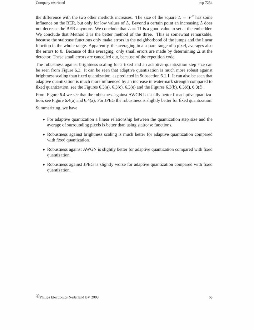
Company restricted rep 7254
the difference with the two other methods increases. The size of the squareL = F 2 has someinfluence on the BER, but only for low values ofL. Beyond a certain point an increasingL doesnot decrease the BER anymore. We conclude thatL = 11 is a good value to set at the embedder.We conclude that Method 3 is the better method of the three. This is somewhat remarkable,because the staircase functions only make errors in the neighborhood of the jumps and the linearfunction in the whole range. Apparently, the averaging in a square range of a pixel, averages alsothe errors to 0. Because of this averaging, only small errors are made by determining∆ at thedetector. These small errors are cancelled out, because of the repetition code.
The robustness against brightness scaling for a fixed and an adaptive quantization step size canbe seen from Figure6.3. It can be seen that adaptive quantization is much more robust againstbrightness scaling than fixed quantization, as predicted in Subsection6.1.1. It can also be seen thatadaptive quantization is much more influenced by an increase in watermark strength compared tofixed quantization, see the Figures6.3(a), 6.3(c), 6.3(e)and the Figures6.3(b), 6.3(d), 6.3(f).
From Figure6.4we see that the robustness against AWGN is usually better for adaptive quantiza-tion, see Figure6.4(a)and6.4(a). For JPEG the robustness is slightly better for fixed quantization.
Summarizing, we have
• For adaptive quantization a linear relationship between the quantization step size and theaverage of surrounding pixels is better than using staircase functions.
• Robustness against brightness scaling is much better for adaptive quantization comparedwith fixed quantization.
• Robustness against AWGN is slightly better for adaptive quantization compared with fixedquantization.
• Robustness against JPEG is slightly worse for adaptive quantization compared with fixedquantization.
c©Philips Electronics Nederland BV 2003 65

rep 7254 Company restricted
adaptive∆fixed∆
BE
R
scaling factor
0
0.1
0.2
0.3
0.4
0.5
0.6
0.7
0.75 0.8 0.85 0.9 0.95 1 1.05 1.1 1.15 1.2 1.25
(a) Repetition coding with DWR = 30 and rate = 0.01.
adaptive∆fixed∆
BE
R
scaling factor
0
0.1
0.2
0.3
0.4
0.5
0.6
0.7
0.75 0.8 0.85 0.9 0.95 1 1.05 1.1 1.15 1.2 1.25
(b) Concatenated coding with DWR = 30 and rate = 0.01.
adaptive∆fixed∆
BE
R
scaling factor
0
0.1
0.2
0.3
0.4
0.5
0.6
0.7
0.75 0.8 0.85 0.9 0.95 1 1.05 1.1 1.15 1.2 1.25
(c) Repetition coding with DWR = 25 and rate = 0.01.
adaptive∆fixed∆
BE
R
scaling factor
0
0.1
0.2
0.3
0.4
0.5
0.6
0.7
0.75 0.8 0.85 0.9 0.95 1 1.05 1.1 1.15 1.2 1.25
(d) Concatenated coding with DWR = 25 and rate = 0.01.
adaptive∆fixed∆
BE
R
scaling factor
0
0.1
0.2
0.3
0.4
0.5
0.6
0.7
0.75 0.8 0.85 0.9 0.95 1 1.05 1.1 1.15 1.2 1.25
(e) Repetition coding with DWR = 20 and rate = 0.01.
adaptive∆fixed∆
BE
R
scaling factor
0
0.1
0.2
0.3
0.4
0.5
0.6
0.7
0.75 0.8 0.85 0.9 0.95 1 1.05 1.1 1.15 1.2 1.25
(f) Concatenated coding with DWR = 20 and rate = 0.01.
Figure 6.3: Adaptive quantization versus fixed quantization. The BER as a function of the bright-ness scaling factor.
66 c©Philips Electronics Nederland BV 2003

Company restricted rep 7254
adaptive∆fixed∆
BE
R
σ2n
00
0.1
0.2
0.3
0.4
0.5
10 20 30 40 50 60
(a) Repetition coding with rate = 0.1 and AWGN attack.
adaptive∆fixed∆
BE
RJPEG quality factor
0
0.1
0.2
0.3
0.4
0.5
60 65 70 75 80 85 90
(b) Repetition coding with rate = 0.1 and JPEG attack.
adaptive∆fixed∆
BE
R
σ2n
00
0.1
0.2
0.3
0.4
0.5
10 20 30 40 50 60
(c) Concatenated coding with rate = 0.01 and AWGN at-tack.
adaptive∆fixed∆
BE
R
JPEG quality factor
0
0.1
0.2
0.3
0.4
0.5
60 65 70 75 80 85 90
(d) Concatenated coding with rate = 0.01 and JPEG attack.
Figure 6.4: Adaptive quantization versus fixed quantization. The BER as a function of the AWGNvariance or the JPEG quality factor.
c©Philips Electronics Nederland BV 2003 67

rep 7254 Company restricted
68 c©Philips Electronics Nederland BV 2003
Chapter 7
Performance analysis
As seen in Chapter4, this report seeks an increased robustness and a performance evaluation of thedeveloped model. Robustness is searched especially for lossy compression and noise attacks. Inthis chapter these attacks are modelled by Additive White Gaussian Noise (AWGN) and uniformlydistributed noise attacks. This model is not very good, because JPEG noise is highly correlatedwith the host signal. Of course, analysis of the effect of noise attacks is made easier if the relevantsignals are assumed to be Gaussian distributed.
The effect of the two improvements over Scalar Costa Scheme (SCS), the use of Error CorrectingCodes (ECC) and an adaptive∆, are to be measured. For ECC this is only done by experiment, seeSection5.4. The improvements of an adaptive quantization step size is measured experimentally inSection6.3. From Subsection6.1.2it is known that using an adaptive∆ introduces an additionalsource of errors, due to the necessity to estimate∆ from the received signal. In this chapter also atheoretical model is developed in order to estimate this error probability.
In Section7.1 a performance measure is given. The error probability for Gaussian and uniformnoise attacks is determined in Section7.2. In Section7.3the error probability due to the use of anadaptive quantization step size is modelled. Finally, in Section7.4 the results are discussed andsummarized.
7.1 A measure for the performance
The performance of a watermarking scheme is measured by the bit error probability. This is theprobability that if a bit (0 or 1) is sent, a wrong bit is detected (1 or 0), i.e., the bit error probabilityis P (mi �= mi). Another performance measure is the message error probabilityP (m �= m).These two performance measures are related byP (m �= m) = 1 − Πl
i=1 (1 − P (mi �= mi)), ifthemi are mutual independent.
A watermarking scheme can also be evaluated by looking at the capacity or the rate-distortionfunction. The capacity of a watermarking channel and the error probability of that channel arerelated. This can be understood intuitively as follows; If the capacity of a channel increases, thenit is possible to embed more bits, or to use this extra space to add redundancy. This additionalredundancy decreases the bit error probability.
The bit error probability is used in order to determine the performance of a watermarking scheme.
69

rep 7254 Company restricted
1Q∆(x) − 14∆ Q∆(x) + 1
4∆
0 1 0
0 0
∆
y
α = 0
α = 0.75
α = 1
x
r1 = y + n r2 = y + n
Q∆(x)
Figure 7.1: The embedding process for embedding 1. Everything in the range[Q∆(x) −12∆, Q∆(x) + 1
2∆] is projected onQ∆(x) for α = 1 and on[Q∆(x) − 12(1 − α)∆, Q∆(x) +
12(1 − α)∆] for α ∈]0, 1[. If, after a noise attack,r = y + n is still in the correct quantizationbin, i.e.,r ∈ [Q∆(x) − 1
4∆, Q∆(x) + 14∆], the received valuer is still in the detection area, and
no error is made. For the noise illustrated by the left red arrow (r1) an error will be made, for theright red arrow (r2) a correct detection is made.
7.2 The bit error probability due to a noise attack
In this section the bit error probability for the SCS is determined. A fixed quantization step size isused and the noise is assumed to be Gaussian or uniformly distributed. Error correction codes canbring the bit error probability down, but for the sake of simple analysis they are not considered.
If the SCS is used, the embedding formula is Equation (3.17). Consider a pixelx. Withoutdistortion compensation (α = 1) embedding is done by quantizingx to the nearest odd or evenlevel (1 or 0, respectively). With distortion compensation (α ∈]0, 1[), the pixel valuex is alteredto a valuey somewhere between the original valuex and the quantized valueQ∆(x). See Figure7.1 for illustration. A correct detection is made wheneverr is in the correct quantization bin,corresponding to 0 or 1.
Assume that the image datax is uniformly distributed over the range of a quantization bin. Ac-cording to [17] this is a reasonable assumption, because in most watermarking applications, thehost-data power is much stronger than the watermark power (σ2
X � σ2W ). If the dither is cho-
sen appropriately,x can be made to be uniformly distributed over a quantization bin [20, 24, 31].The added noise is assumed to be either normally distributed with zero mean and varianceσ2
N oruniformly distributed on[−c, c], so
NU ∼ U [−c, c], pNU (n) =
{12c if n ∈ [−c, c]0 otherwise
(7.1)
NG ∼ N(0, σ2n), pNG(n) =
1√2πσn
en2
2σ2n ,∀n ∈ R. (7.2)
70 c©Philips Electronics Nederland BV 2003
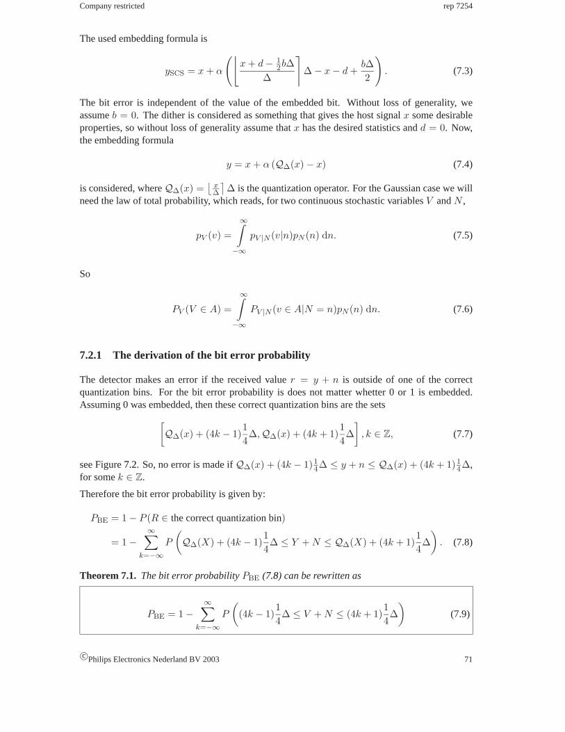
Company restricted rep 7254
The used embedding formula is
ySCS = x + α
(⌊x + d − 1
2b∆∆
⌉∆ − x − d +
b∆2
). (7.3)
The bit error is independent of the value of the embedded bit. Without loss of generality, weassumeb = 0. The dither is considered as something that gives the host signalx some desirableproperties, so without loss of generality assume thatx has the desired statistics andd = 0. Now,the embedding formula
y = x + α (Q∆(x) − x) (7.4)
is considered, whereQ∆(x) =⌊
x∆
⌉∆ is the quantization operator. For the Gaussian case we will
need the law of total probability, which reads, for two continuous stochastic variablesV andN ,
pV (v) =
∞∫−∞
pV |N (v|n)pN (n) dn. (7.5)
So
PV (V ∈ A) =
∞∫−∞
PV |N (v ∈ A|N = n)pN (n) dn. (7.6)
7.2.1 The derivation of the bit error probability
The detector makes an error if the received valuer = y + n is outside of one of the correctquantization bins. For the bit error probability is does not matter whetter 0 or 1 is embedded.Assuming 0 was embedded, then these correct quantization bins are the sets[
Q∆(x) + (4k − 1)14∆,Q∆(x) + (4k + 1)
14∆]
, k ∈ Z, (7.7)
see Figure7.2. So, no error is made ifQ∆(x) + (4k − 1)14∆ ≤ y + n ≤ Q∆(x) + (4k + 1)1
4∆,for somek ∈ Z.
Therefore the bit error probability is given by:
PBE = 1 − P (R ∈ the correct quantization bin)
= 1 −∞∑
k=−∞P
(Q∆(X) + (4k − 1)
14∆ ≤ Y + N ≤ Q∆(X) + (4k + 1)
14∆)
. (7.8)
Theorem 7.1. The bit error probabilityPBE (7.8) can be rewritten as
PBE = 1 −∞∑
k=−∞P
((4k − 1)
14∆ ≤ V + N ≤ (4k + 1)
14∆)
(7.9)
c©Philips Electronics Nederland BV 2003 71
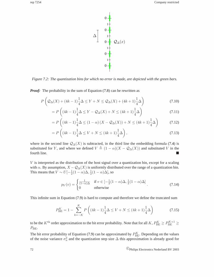
rep 7254 Company restricted
0
1
0
0
1
1
1
0
0
∆
Q∆(x)
Figure 7.2: The quantization bins for which no error is made, are depicted with the green bars.
Proof: The probability in the sum of Equation (7.8) can be rewritten as
P
(Q∆(X) + (4k − 1)
14∆ ≤ Y + N ≤ Q∆(X) + (4k + 1)
14∆)
(7.10)
= P
((4k − 1)
14∆ ≤ Y −Q∆(X) + N ≤ (4k + 1)
14∆)
(7.11)
= P
((4k − 1)
14∆ ≤ (1 − α) (X −Q∆(X)) + N ≤ (4k + 1)
14∆)
(7.12)
= P
((4k − 1)
14∆ ≤ V + N ≤ (4k + 1)
14∆)
, (7.13)
where in the second lineQ∆(X) is subtracted, in the third line the embedding formula (7.4) issubstituted forY , and where we definedV � (1 − α)(X − Q∆(X)) and substitutedV in thefourth line. �
V is interpreted as the distribution of the host signal over a quantization bin, except for a scalingwith α. By assumption,X −Q∆(X) is uniformly distributed over the range of a quantization bin.This means thatV ∼ U [−1
2(1 − α)∆, 12(1 − α)∆], so
pV (v) =
{1
(1−α)∆ if v ∈ [−12(1 − α)∆, 1
2(1 − α)∆]
0 otherwise. (7.14)
This infinite sum in Equation (7.9) is hard to compute and therefore we define the truncated sum
PKBE = 1 −
K∑k=−K
P
((4k − 1)
14∆ ≤ V + N ≤ (4k + 1)
14∆)
(7.15)
to be theKth order approximation to the bit error probability. Note that for allK, PKBE ≥ PK+1
BE ≥PBE.
The bit error probability of Equation (7.9) can be approximated byPKBE. Depending on the values
of the noise varianceσ2n and the quantization step size∆ this approximation is already good for
72 c©Philips Electronics Nederland BV 2003
Company restricted rep 7254
K = 1, because for moderate noise the probability thatr will come in another quantization bin, isvery small. So, the0th order approximation for the bit error probabilityPBE, as given by
P 0BE = 1 − P
(−1
4∆ ≤ V + N ≤ 1
4∆)
(7.16)
= P
(|V + N | >
14∆)
, (7.17)
may already give relevant information. A better approximation is given by
P 1BE = 1 − P
(−1
4∆ ≤ V + N ≤ 1
4∆)− P
(−5
4∆ ≤ V + N ≤ −3
4∆)
− P
(34∆ ≤ V + N ≤ 5
4∆) (7.18)
= P 0BE − P
(−5
4∆ ≤ V + N ≤ −3
4∆)− P
(34∆ ≤ V + N ≤ 5
4∆)
. (7.19)
The two cases of AWGN and uniformly distributed noise, i.e.,NG ∼ N(0, σ2N ) and NU ∼
U [−c, c], are considered in the following two sections. There we will derive formulas for the biterror probability.
7.2.2 The bit error probability for Gaussian noise
In this subsection the bit error probability for the Gaussian case is approximated withP 0BE and
P 1BE. In the following theorems the formulas forP 0
BE andP 1BE are derived.
The following facts about the error function erf and the complementary error function erfc areused
erf(z) = 1 − erfc(z), (7.20)
erf(−z) = − erf(z), (7.21)∫erf(z) dz = z erf(z) +
1√π
e−z2. (7.22)
Theorem 7.2. For α = 1,
P 0BE = 1 − erf
(14∆√2 σn
). (7.23)
Proof: For the case of no distortion compensation,α = 1, the host signal is quantized to onepoint, sov = 0. Using Equation (7.16) P 0
BE is calculated as
P 0BE = 1 −
∆4∫
−∆4
1√2πσn
en2
2σ2n dn,
This is equal to (7.23), where (7.20) and (7.21) are used. �
c©Philips Electronics Nederland BV 2003 73
rep 7254 Company restricted
Theorem 7.3. For 0 < α < 1 we have
P 0BE =
α − 12
2(1 − α)erf
(12(α − 1
2)∆√2σn
)− α − 3
2
2(1 − α)erf
(12(α − 3
2)∆√2σn
)
+2σn√
2π(1 − α)∆
(e−
14 (α− 1
2 )2∆2
2σ2n − e
−14 (α− 3
2 )2∆2
2σ2n
)+ 1.
(7.24)
Proof: Using distortion compensation,α ∈]0, 1[, v is distributed with a probability density func-tion as in Equation (7.14). The approximation of the conditional bit error probability givenvis
P (BE | V = v) = P (|V + NG| >∆4
| V = v) (7.25)
= P (NG >∆4− V | V = v) + P (NG < −∆
4− V | V = v) (7.26)
=
∞∫∆4−v
pNG(n) dn +
−∆4−v∫
−∞pNG(n) dn. (7.27)
Then we apply the law of total probability (see (7.6)), to obtain
P 0BE =
12(1−α)∆∫
− 12(1−α)∆
P (BE | V = v)pV (v) dv
=
12(1−α)∆∫
− 12(1−α)∆
∞∫∆4−v
1√2πσn
e−n2
2σ2n dn +
−∆4−v∫
−∞
1√2πσn
e−n2
2σ2n dn
1
(1 − α)∆dv
=
12(1−α)∆∫
− 12(1−α)∆
[12
erfc
(14∆ − v√
2σn
)+
(1 − 1
2erfc
(−1
4∆ − v√2σn
))]1
(1 − α)∆dv, (7.28)
where we used (7.2) and (7.14). In order to rewrite Equation (7.28), the Equations (7.20), (7.21)and (7.22) are used. NowP 0
BE can be rewritten as
P 0BE = c0
b∫a
1 dv − 12c0
b∫a
erf
(14∆ − v√
2σn
)dv +
12c0
b∫a
erf
(−1
4∆ − v√2σn
)dv, (7.29)
with c0 = 1(1−α)∆ , a = −1
2(1 − α)∆ andb = 12(1 − α)∆ and where we used (7.20). The first
74 c©Philips Electronics Nederland BV 2003
Company restricted rep 7254
integral is equal to1c0
. The second is equal to
b∫a
erf
(14∆ − v√
2σn
)dv = −
√2σn
b∫a
erf(u) du = −√
2σn
[u erf(u) +
1√π
e−u2
]u=b
a
(7.30)
= −12(α − 1
2)∆ erf
(12(α − 1
2)∆√2σn
)−
√2σn√π
e−
14 (α− 1
2 )2∆2
2σ2n
+12(α − 3
2)∆ erf
(12(α − 3
2)∆√2σn
)+
√2σn√π
e−
14 (α− 3
2 )2∆2
2σ2n ,
(7.31)
where in the first line the integration variablev is changed intou, with u =14∆−v√2σn
, a =14∆−a√2σn
,
b =14∆−b√2σn
, and where also in the first line Equation (7.22) is applied. In the second line the
expression is evaluated fora andb.
The same procedure is applied on the third integral. Taking the three integrals together again andusing Equation (7.21) gives the desired result. �
A better approximation can be calculated withP 1BE, see Equation (7.19).
Theorem 7.4. For α = 1
P 1BE = 1 − erf
(14∆√2 σn
)+ erf
(34∆√2 σn
)− erf
(54∆√2 σn
). (7.32)
Proof: Use (7.19), v = 0 and apply the same reasoning as in Theorem7.2. �
Theorem 7.5. For 0 < α < 1 we have
P 1BE =
α − 12
2(1 − α)erf
(12(α − 1
2)∆√2σn
)− α − 3
2
2(1 − α)erf
(12(α − 3
2)∆√2σn
)
+α − 5
2
2(1 − α)erf
(12(α − 5
2)∆√2σn
)− α − 7
2
2(1 − α)erf
(12(α − 7
2)∆√2σn
)
− α + 12
2(1 − α)erf
(12(α + 1
2)∆√2σn
)+
α + 32
2(1 − α)erf
(12(α + 3
2)∆√2σn
)
+2σn√
2π(1 − α)∆
(− e
−14 (α− 7
2 )2∆2
2σ2n + e
−14 (α− 5
2 )2∆2
2σ2n − e
−14 (α− 3
2 )2∆2
2σ2n
+ e−
14 (α− 1
2 )2∆2
2σ2n − e
−14 (α+1
2 )2∆2
2σ2n + e
−14 (α+3
2 )2∆2
2σ2n
)+ 1.
(7.33)
Proof: With (7.18) the conditional bit error probability givenV = v can be made. Applying the
c©Philips Electronics Nederland BV 2003 75

rep 7254 Company restricted
law of total probability and after some rewriting, as in the caseP 0BE, we get
P 1BE = c0
b∫a
1 dv +12c0
b∫a
erf
(−1
4∆ − v√2σn
)dv − 1
2c0
b∫a
erf
(14∆ − v√
2σn
)dv
+12c0
b∫a
erf
(−5
4∆ − v√2σn
)dv − 1
2c0
b∫a
erf
(−3
4∆ − v√2σn
)dv
+12c0
b∫a
erf
(34∆ − v√
2σn
)dv − 1
2c0
b∫a
erf
(54∆ − v√
2σn
)dv,
(7.34)
with c0, a andb as before.
Following the same procedure as with the calculation ofP 0BE for 0 < α < 1, this gives the desired
result. �
The0th order approximation for the case of Gaussian noise (7.24) is drawn as a function ofα fordifferent WNR’s in Figure8.1.
7.2.3 The bit error probability for uniform noise
Next, we will compute approximations to the bit error probability (7.9) for the case of uniformlydistributed noiseN and ”host”V . In order to establish the bit error probability, first the distributionof the sumV + N of the two uniform distributed variablesV andN is calculated. We have thatN ∼ U [−c, c] (7.1) andV ∼ U [−1
2(1 − α)∆, 12(1 − α)∆] (7.14). A distinction is made between
two cases:
Weak noise case: The noise variance is smaller than the variance ofV : σ2N ≤ σ2
V or c ≤ 12(1 −
α)∆;
Strong noise case: The variance ofV is smaller than the noise variance:σ2N > σ2
V or c >12(1 − α)∆.
In this subsection we will treat the weak noise case. The strong noise case can be treated com-pletely analogously, so only the results are stated. See Figure7.3for the probability density func-tions ofV , N and the sumZ = V + N for the weak noise case. In the following the probabilitydensity function ofZ is derived.
76 c©Philips Electronics Nederland BV 2003

Company restricted rep 7254
v0
pZ = pV +N
n0 n1 v1v0 + n0 0 v1 + n1v0 + n1 v1 + n0
1v1−v0
n0 0 n1 v1v0
1v1−v0
1n1−n0
pNpV
Figure 7.3: The probability density functions ofN , V and the sumZ for the weak noise case:σ2
N ≤ σ2V .
Theorem 7.6. The probability density function ofZ for the weak noise case is given by
pZ(z) =
z−(v0+n0)(v1−v0)(n1−n0) if z > v0 + n0 andz ≤ v0 + n1
1(v1−v0) if z > v0 + n1 andz ≤ v1 + n0
(v1+n1)−z(v1−v0)(n1−n0) if z > v1 + n0 andz ≤ v1 + n1
0 otherwise
(7.35)
=
z+ 12(1−α)∆+c
2(1−α)∆c if −12(1 − α)∆ − c ≤ z ≤ −1
2(1 − α)∆ + c1
(1−α)∆ if −12(1 − α)∆ + c ≤ z ≤ 1
2(1 − α)∆ − c12(1−α)∆+c−z
2(1−α)∆c if 12(1 − α)∆ − c ≤ z ≤ 1
2(1 − α)∆ + c
0 otherwise
(7.36)
Proof: Consider the general case thatV ∼ U [y0, y1] andN ∼ U [n0, n1]. The weak noise case isdivided again in three subcases: subcase A1 is the casez ≤ v0 + n1 (this is area 1 in Figure7.4),subcase A2 is the casez > v0 + n1 andz ≤ v1 + n0 (this is area 2), and subcase A3 is the casez > v1 + n0 (area 3).
In order to calculate the probability ofZ ≤ z integration is done over areai for subcase Ai,i = 1, 2, 3. Subcase A1 gives
P (Z ≤ z) =
z−n0∫v0
z−v∫n0
1(v1 − v0)
1(n1 − n0)
dn dv =
z−n0∫v0
z − v − n0
(v1 − v0)(n1 − n0)dv (7.37)
=12
(z − n0)2
(v1 − v0)(n1 − n0)+
12v2
0 − v0(z − n0)(v1 − v0)(n1 − n0)
, (7.38)
c©Philips Electronics Nederland BV 2003 77

rep 7254 Company restricted
2
3
1
1
2
3
(v1, n0)n0
v0
(v0, n0)
v1
n1
(v1, n1)(v0, n1)
(z − n0, n0)
(z − n1, n1)
z = v0 + n1
z = v1 + n0
:
{z − n0 ≤ v ≤ z − n1
n0 ≤ n ≤ z − v
:
{z − n1 ≤ v ≤ v1
n0 ≤ n ≤ z − v
:
{v0 ≤ v ≤ z − n0
n0 ≤ n ≤ z − v
Figure 7.4: The integration areas of the three subcases of the weak noise case.
for subcase A2
P (Z ≤ z) =
z−n1∫v0
n1∫n0
1(v1 − v0)
1(n1 − n0)
dn dv +
z−n0∫z−n1
z−v∫n0
1(v1 − v0)
1(n1 − n0)
dn dv
(7.39)
=z − n1 − v0
(v1 − v0)+
z−n0∫z−n1
z − v − n0
(v1 − v0)(n1 − n0)dv (7.40)
=12(n1 − n0)2
(v1 − v0)(n1 − n0)+
z − (n1 + v0)(v1 − v0)
, (7.41)
and for subcase A3
P (Z ≤ z) =
z−n1∫v0
n1∫n0
1(v1 − v0)
1(n1 − n0)
dn dv +
v1∫z−n1
z−v∫n0
1(v1 − v0)
1(n1 − n0)
dn dv
(7.42)
=z − n1 − v0
(v1 − v0)+
v1∫z−n1
z − v − n0
(v1 − v0)(n1 − n0)dv (7.43)
=z − (n1 + v0)
(v1 − v0)+
(z − n0)(v1 + n1 − z) + 12(z − n1)2 − 1
2v21
(v1 − v0)(n1 − n0). (7.44)
The probability density function ofZ for the weak noise case is given bypZ(z) = ddzP (Z ≤ z).
For our case we havev0 = −12(1−α)∆, v1 = 1
2(1−α)∆, n0 = −c andn1 = c, which completesthe proof. �
78 c©Philips Electronics Nederland BV 2003
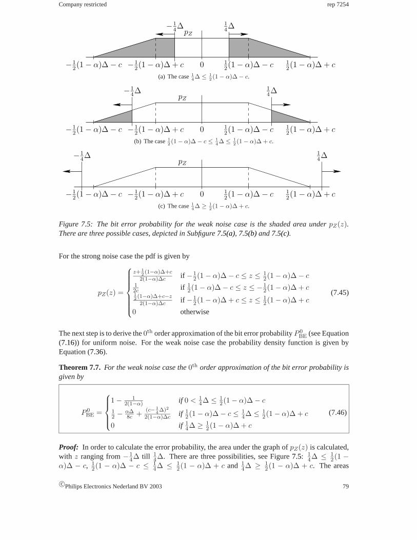
Company restricted rep 7254
0
−14∆ 1
4∆
−12(1 − α)∆ − c −1
2(1 − α)∆ + c 1
2(1 − α)∆ − c 1
2(1 − α)∆ + c
pZ
(a) The case14∆ ≤ 1
2(1 − α)∆ − c.
pZ
−12(1 − α)∆ − c −1
2(1 − α)∆ + c 1
2(1 − α)∆ + c
−14∆ 1
4∆
12(1 − α)∆ − c0
(b) The case12(1 − α)∆ − c ≤ 1
4∆ ≤ 1
2(1 − α)∆ + c.
pZ
−12(1 − α)∆ − c −1
2(1 − α)∆ + c 1
2(1 − α)∆ − c 1
2(1 − α)∆ + c
−14∆ 1
4∆
0
(c) The case14∆ ≥ 1
2(1 − α)∆ + c.
Figure 7.5: The bit error probability for the weak noise case is the shaded area underpZ(z).There are three possible cases, depicted in Subfigure7.5(a), 7.5(b)and7.5(c).
For the strong noise case the pdf is given by
pZ(z) =
z+ 12(1−α)∆+c
2(1−α)∆c if −12(1 − α)∆ − c ≤ z ≤ 1
2(1 − α)∆ − c12c if 1
2(1 − α)∆ − c ≤ z ≤ −12(1 − α)∆ + c
12(1−α)∆+c−z
2(1−α)∆c if −12(1 − α)∆ + c ≤ z ≤ 1
2(1 − α)∆ + c
0 otherwise
(7.45)
The next step is to derive the0th order approximation of the bit error probabilityP 0BE (see Equation
(7.16)) for uniform noise. For the weak noise case the probability density function is given byEquation (7.36).
Theorem 7.7. For the weak noise case the0th order approximation of the bit error probability isgiven by
P 0BE =
1 − 12(1−α) if 0 < 1
4∆ ≤ 12(1 − α)∆ − c
12 − α∆
8c + (c− 14∆)2
2(1−α)∆c if 12(1 − α)∆ − c ≤ 1
4∆ ≤ 12(1 − α)∆ + c
0 if 14∆ ≥ 1
2(1 − α)∆ + c
(7.46)
Proof: In order to calculate the error probability, the area under the graph ofpZ(z) is calculated,with z ranging from−1
4∆ till 14∆. There are three possibilities, see Figure7.5: 1
4∆ ≤ 12(1 −
α)∆ − c, 12(1 − α)∆ − c ≤ 1
4∆ ≤ 12(1 − α)∆ + c and 1
4∆ ≥ 12(1 − α)∆ + c. The areas
c©Philips Electronics Nederland BV 2003 79
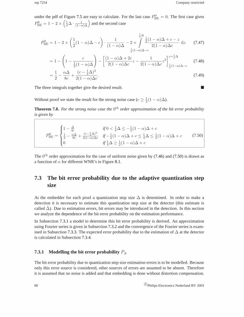
rep 7254 Company restricted
under the pdf of Figure7.5 are easy to calculate. For the last caseP 0BE = 0. The first case gives
P 0BE = 1 − 2 ×
(14∆ · 1
(1−α)∆
)and the second case
P 0BE = 1 − 2 ×
(12(1 − α)∆ − c
)· 1(1 − α)∆
− 2 ×14∆∫
12(1−α)∆−c
12(1 − α)∆ + c − z
2(1 − α)∆cdz (7.47)
= 1 −(
1 − c12(1 − α)∆
)−[(1 − α)∆ + 2c
2(1 − α)∆cz − 1
2(1 − α)∆cz2
]z= 14∆
12(1−α)∆−c
(7.48)
=12− α∆
8c+
(c − 14∆)2
2(1 − α)∆c. (7.49)
The three integrals together give the desired result. �
Without proof we state the result for the strong noise case (c ≥ 12(1 − α)∆).
Theorem 7.8. For the strong noise case the0th order approximation of the bit error probabilityis given by
P 0BE =
1 − ∆4c if 0 < 1
4∆ ≤ −12(1 − α)∆ + c
12 − α∆
8c + (c− 14∆)2
2(1−α)∆c if −12(1 − α)∆ + c ≤ 1
4∆ ≤ 12(1 − α)∆ + c
0 if 14∆ ≥ 1
2(1 − α)∆ + c
(7.50)
The0th order approximation for the case of uniform noise given by (7.46) and (7.50) is drawn asa function ofα for different WNR’s in Figure8.1.
7.3 The bit error probability due to the adaptive quantization stepsize
At the embedder for each pixel a quantization step size∆ is determined. In order to make adetection it is necessary to estimate this quantization step size at the detector (this estimate iscalled∆). Due to estimation errors, bit errors may be introduced in the detection. In this sectionwe analyze the dependence of the bit error probability on the estimation performance.
In Subsection7.3.1a model to determine this bit error probability is derived. An approximationusing Fourier series is given in Subsection7.3.2and the convergence of the Fourier series is exam-ined in Subsection7.3.3. The expected error probability due to the estimation of∆ at the detectoris calculated in Subsection7.3.4.
7.3.1 Modelling the bit error probability P∆
The bit error probability due to quantization step size estimation errors is to be modelled. Becauseonly this error source is considered, other sources of errors are assumed to be absent. Thereforeit is assumed that no noise is added and that embedding is done without distortion compensation.
80 c©Philips Electronics Nederland BV 2003

Company restricted rep 7254
A
32∆
f∆(z)
012∆ ∆ 3
2∆ 2∆ 5
2∆
1
-1
0
1
-1
f ∆(z)
12∆ ∆ 2∆
0
1
-1
f∆(z) × f ∆(z)
z
z
z
= error
3∆
52∆
B
Figure 7.6: The detection error made due to the errors in the estimation of the quantization stepsize. In the upper and middle plots detection with∆ and∆, respectively, is shown. The values ofz for which an error is made is shown in the lower plot, which is a plot of the product off∆(z)andf ∆(z).
For simplicity, we also assume that the dither equals zero. The bit error probability due to theestimation of the adaptive quantization step size at the detector is denoted byP∆.
Consider Figure7.6. This shows for some quantization step size which bit is detected, dependingon the pixel valuez. The upper plot of Figure7.6 shows which bit is detected if the correctquantization step size∆ is used, that is if at the detector the quantization step size is estimatedcorrectly (∆ = ∆). We call this functionf∆(z), with
f∆(z) = sign
(− cos
(π
12∆
z
))(7.51)
wheresign(z) � z|z| if z �= 0 andsign(z) = 0 if z = 0. The middle plot of Figure7.6 shows
detection with an estimated∆ which is slightly bigger than the quantization step size∆ used atthe embedding side. This function is calledf ∆(z). An error is made for all pixel valuesz for
whichf∆(z) �= f ∆(z), i.e., for which the productf∆(z)× f ∆(z) equals -1, see the lower plot ofFigure7.6.
For ease of computation, we scale the variablez, and all related variables (∆ and∆), such that
c©Philips Electronics Nederland BV 2003 81

rep 7254 Company restricted
the range ofz becomes the interval[0, 1]. The probability that an error will be made is equal to
the area between the graph off∆(z) × f ∆(z) and the horizontal liney = 0. If we call the areacorresponding to correct detectionA (the white area in Figure7.6) and the area corresponding toerroneous detectionB (the shaded area in Figure7.6), then we have:
A + B = 1, (7.52)1∫
0
(f∆(z) × f ∆(z)
)pz(z) dz = A − B, (7.53)
wherepz(z) is the pdf ofz. Then the bit error probability equals:
P∆ = B =12− 1
2
1∫0
(f∆(z) × f ∆(z)
)pz(z) dz (7.54)
=12− 1
2
1∫0
sign(
cos( π
∆z)
cos(
π
∆z
))pz(z) dz. (7.55)
Plots for this bit error probabilityP∆ are given in AppendixC. From these plot it is clear that thequantization step size should be estimated with large precision, because elseP∆ increases rapidly.
This integral is very hard to evaluate due to thesign-function. Therefore, we have to approximatethe integral. We do this in the next subsection by approximating the functionsf∆(z) andf ∆(z)by their Fourier series.
7.3.2 Fourier approximation
Note thatf∆(z) is a periodic function with period∆. This function can be approximated by theFourier series on[−1
2∆, 12∆]. According to Fourier theory the Fourier series off∆(z) is given by
∞∑i=0
αigi(z), (7.56)
whereS = {g0(z), g1(z), · · · } is an orthonormal system in the Hilbert spaceH of squared in-tegrable functions on[−1
2∆, 12∆] and whereαi = 〈f, gi(z)〉, with 〈·〉 an inner product. The
L2-norm on[−12∆, 1
2∆] is used, which is
‖f‖[− 12∆, 1
2∆]
2 =
1
12∆
12∆∫
− 12∆
|f(z)|2 dz
12
(7.57)
and is derived from the inner product
〈f, g〉[− 12∆, 1
2∆] =
112∆
12∆∫
− 12∆
|f(z)g(z)| dz. (7.58)
82 c©Philips Electronics Nederland BV 2003
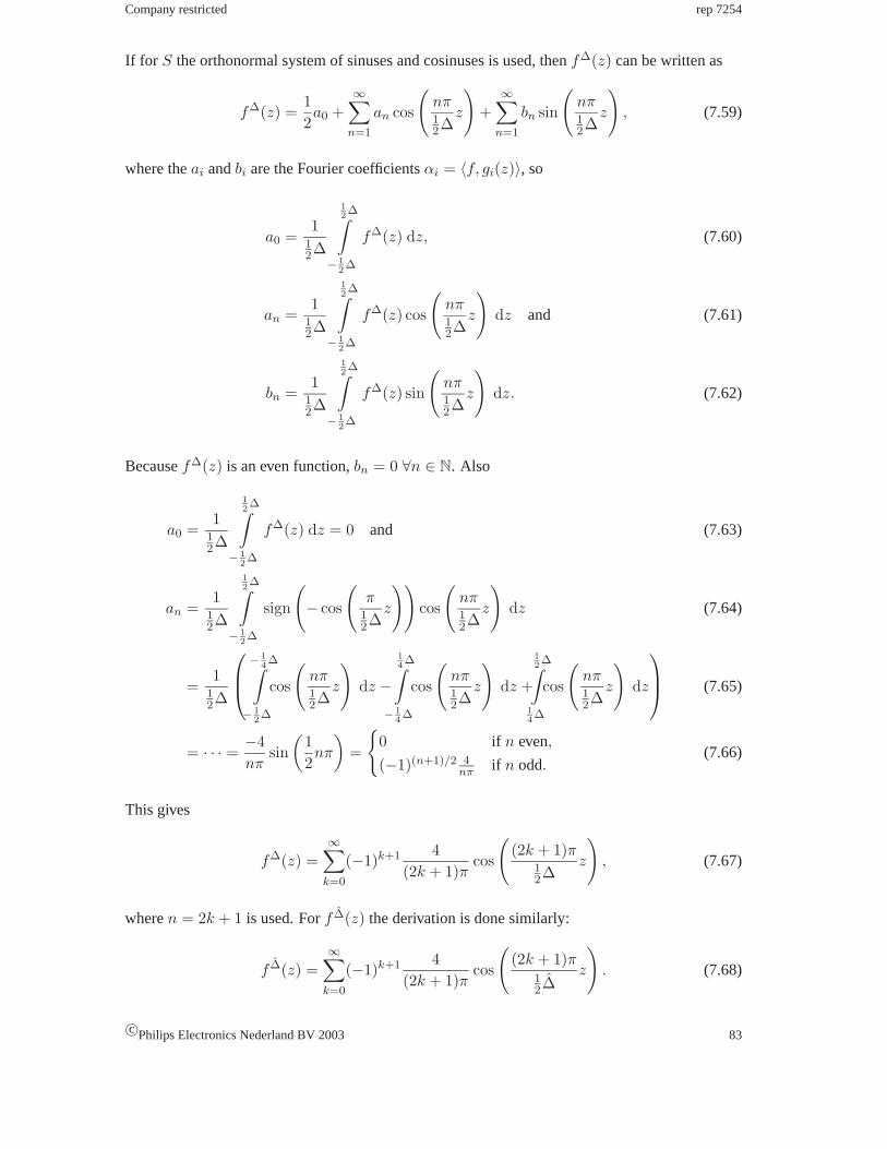
Company restricted rep 7254
If for S the orthonormal system of sinuses and cosinuses is used, thenf∆(z) can be written as
f∆(z) =12a0 +
∞∑n=1
an cos
(nπ12∆
z
)+
∞∑n=1
bn sin
(nπ12∆
z
), (7.59)
where theai andbi are the Fourier coefficientsαi = 〈f, gi(z)〉, so
a0 =1
12∆
12∆∫
− 12∆
f∆(z) dz, (7.60)
an =1
12∆
12∆∫
− 12∆
f∆(z) cos
(nπ12∆
z
)dz and (7.61)
bn =1
12∆
12∆∫
− 12∆
f∆(z) sin
(nπ12∆
z
)dz. (7.62)
Becausef∆(z) is an even function,bn = 0 ∀n ∈ N. Also
a0 =1
12∆
12∆∫
− 12∆
f∆(z) dz = 0 and (7.63)
an =1
12∆
12∆∫
− 12∆
sign
(− cos
(π
12∆
z
))cos
(nπ12∆
z
)dz (7.64)
=1
12∆
− 14∆∫
− 12∆
cos
(nπ12∆
z
)dz −
14∆∫
− 14∆
cos
(nπ12∆
z
)dz +
12∆∫
14∆
cos
(nπ12∆
z
)dz
(7.65)
= · · · =−4nπ
sin(
12nπ
)=
{0 if n even,
(−1)(n+1)/2 4nπ if n odd.
(7.66)
This gives
f∆(z) =∞∑
k=0
(−1)k+1 4(2k + 1)π
cos
((2k + 1)π
12∆
z
), (7.67)
wheren = 2k + 1 is used. Forf ∆(z) the derivation is done similarly:
f ∆(z) =∞∑
k=0
(−1)k+1 4(2k + 1)π
cos
((2k + 1)π
12∆
z
). (7.68)
c©Philips Electronics Nederland BV 2003 83

rep 7254 Company restricted
So we have
P∆ =12− 1
2
1∫0
{ ∞∑k=0
(−1)k+1 4(2k + 1)π
cos
((2k + 1)π
12∆
z
)
×∞∑
k=0
(−1)k+1 4(2k + 1)π
cos
((2k + 1)π
12∆
z
)}pz(z)dz.
(7.69)
7.3.3 Convergence analysis
In this subsection the convergence of (7.69) is established. According to Theorem 11.4 of [1] theFourier series of a functionf converges pointwise tof if and only if(
‖f‖[− 12∆, 1
2∆]
2
)2
=∞∑i=1
|αi|2, (7.70)
with αi the Fourier coefficients off and where the L2-norm on[−12∆, 1
2∆] is used. Equation(7.70) is known as Parseval’s formula. Forf∆ this means
(‖f∆‖[− 1
2∆, 1
2∆]
2
)2
=1
12∆
12∆∫
− 12∆
f∆(z)2 dz = 2 (7.71)
(7.72)
and∞∑i=1
|αi|2 =∞∑
k=0
∣∣∣∣(−1)k+1 12k + 1
4π
∣∣∣∣2
=16π2
∞∑k=0
1(2k + 1)2
=16π2
π2
8= 2, (7.73)
from which it can be concluded that the Fourier series off∆(z) and f ∆(z) converges point-
wise tof∆(z) andf ∆(z) respectively. Becausef∆(z) andf ∆(z) are not continuous functions,
their Fourier series does not converge uniformly, see [1]. It is known thatf∆(z) andf ∆(z) arecontinuous on the interval[0, 1], except for some points of discontinuityz = (2k + 1)1
4∆ orz = (2k + 1)1
4∆, k ∈ N. Therefore, we have that their Fourier series are uniform convergent onany closed intervalI ⊂ [0, 1] not containing a point of discontinuity.
According to Theorem 11.4 of [1], because Equation (7.70) holds, it also holds that
limn→∞ ‖f − sn‖[− 1
2∆, 1
2∆]
2 = 0, (7.74)
where{sn} is the sequence of partial sums defined bysn(z) =n∑
k=0
αk gk(z). Becausef∆(z) is a
periodical function, not onlylimn→∞
112∆
∫ 12∆
− 12∆|f∆(z)−sn|2 dz = 0, but also lim
n→∞1
12∆
∫ 32∆
12∆
|f∆(z)−sn|2 dz = 0, and so on. Also,lim
n→∞1
12∆
∫ 12∆
− 12∆|f∆(z)−sn|2 dz = 0 implies lim
n→∞1
12∆
∫ ba |f∆(z)−
sn|2 dz = 0, for a, b ∈ [−12∆, 1
2∆], because the integration term is positive. Therefore
limn→∞ ‖f − sn‖[0,1]
2 = limn→∞ ‖f − sn‖[0, 1
2∆]
2 + limn→∞ ‖f − sn‖[ 1
2∆, 3
2∆]
2
+ · · · + limn→∞ ‖f − sn‖[h,1]
2 = 0,(7.75)
84 c©Philips Electronics Nederland BV 2003
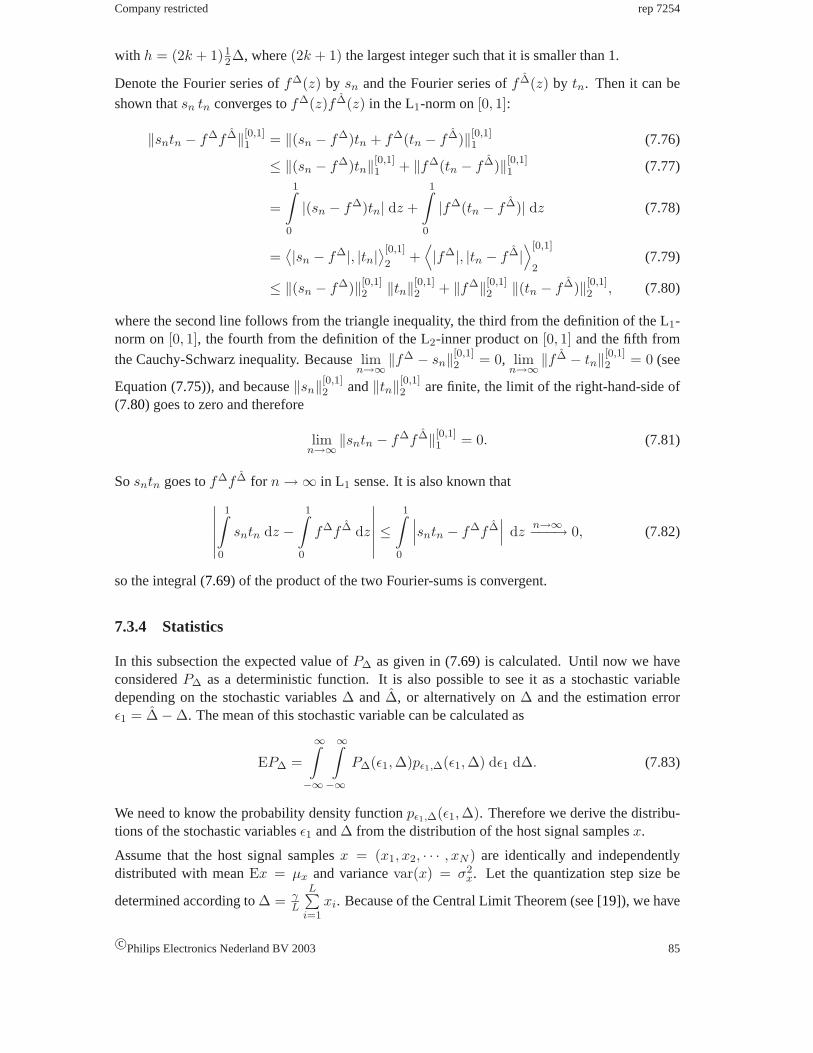
Company restricted rep 7254
with h = (2k + 1)12∆, where(2k + 1) the largest integer such that it is smaller than 1.
Denote the Fourier series off∆(z) by sn and the Fourier series off ∆(z) by tn. Then it can be
shown thatsn tn converges tof∆(z)f ∆(z) in the L1-norm on[0, 1]:
‖sntn − f∆f ∆‖[0,1]1 = ‖(sn − f∆)tn + f∆(tn − f ∆)‖[0,1]
1 (7.76)
≤ ‖(sn − f∆)tn‖[0,1]1 + ‖f∆(tn − f ∆)‖[0,1]
1 (7.77)
=
1∫0
|(sn − f∆)tn| dz +
1∫0
|f∆(tn − f ∆)| dz (7.78)
=⟨|sn − f∆|, |tn|
⟩[0,1]
2+⟨|f∆|, |tn − f ∆|
⟩[0,1]
2(7.79)
≤ ‖(sn − f∆)‖[0,1]2 ‖tn‖[0,1]
2 + ‖f∆‖[0,1]2 ‖(tn − f ∆)‖[0,1]
2 , (7.80)
where the second line follows from the triangle inequality, the third from the definition of the L1-norm on[0, 1], the fourth from the definition of the L2-inner product on[0, 1] and the fifth from
the Cauchy-Schwarz inequality. Becauselimn→∞ ‖f∆ − sn‖[0,1]
2 = 0, limn→∞ ‖f ∆ − tn‖[0,1]
2 = 0 (see
Equation (7.75)), and because‖sn‖[0,1]2 and‖tn‖[0,1]
2 are finite, the limit of the right-hand-side of(7.80) goes to zero and therefore
limn→∞ ‖sntn − f∆f ∆‖[0,1]
1 = 0. (7.81)
Sosntn goes tof∆f ∆ for n → ∞ in L1 sense. It is also known that∣∣∣∣∣∣1∫
0
sntn dz −1∫
0
f∆f ∆ dz
∣∣∣∣∣∣ ≤1∫
0
∣∣∣sntn − f∆f ∆∣∣∣ dz
n→∞−−−→ 0, (7.82)
so the integral (7.69) of the product of the two Fourier-sums is convergent.
7.3.4 Statistics
In this subsection the expected value ofP∆ as given in (7.69) is calculated. Until now we haveconsideredP∆ as a deterministic function. It is also possible to see it as a stochastic variabledepending on the stochastic variables∆ and ∆, or alternatively on∆ and the estimation errorε1 = ∆ − ∆. The mean of this stochastic variable can be calculated as
EP∆ =
∞∫−∞
∞∫−∞
P∆(ε1, ∆)pε1,∆(ε1, ∆) dε1 d∆. (7.83)
We need to know the probability density functionpε1,∆(ε1, ∆). Therefore we derive the distribu-tions of the stochastic variablesε1 and∆ from the distribution of the host signal samplesx.
Assume that the host signal samplesx = (x1, x2, · · · , xN ) are identically and independentlydistributed with meanEx = µx and variancevar(x) = σ2
x. Let the quantization step size be
determined according to∆ = γL
L∑i=1
xi. Because of the Central Limit Theorem (see [19]), we have
c©Philips Electronics Nederland BV 2003 85
rep 7254 Company restricted
for sufficiently largeL thatSL =L∑
i=1xi can be approximated by a normal distribution with mean
µS = E[∑
xi
]=
∑E [xi] = Lµx (7.84)
and variance
σ2S = var
[∑xi
]=
∑var [xi] = Lσ2
x. (7.85)
Hence,∆L = γLSL has a normal distribution, as well, with mean
µ∆ = E[ γ
LSL
]=
γ
LLµx = γµx (7.86)
and variance
σ2∆ = var
[ γ
LSL
]=
γ2
L2var [SL] =
γ2
Lσ2
x. (7.87)
So the probability density function of∆L is given by
p∆(∆) =1√2π
√L
γσxe−L
(∆−γµx)2
2γ2σ2x . (7.88)
By assumption the watermarkw = y − x is uniformly distributed over[−∆, ∆], if α = 1, so
pw|∆(w|∆) =
{1
2∆ if w ∈ [−∆, ∆]0 otherwise
(7.89)
We definedε1 = ∆ − ∆, therefore
ε1 =γ
L
L∑i=1
(yi − xi) =γ
L
L∑i=1
(xi + wi − xi) =γ
L
L∑i=1
wi. (7.90)
We calculate the distribution ofε1 given∆ the same way as we did with calculating the distributionof ∆ and we get thatε1 given∆ is normally distributed with zero mean and varianceγ2∆2
6L , so
pε1|∆(ε1) =1√2π
√6L
γ∆e−6L
ε212γ2∆2 (7.91)
Using the definition of conditional probabilities we have
pε1,∆(ε1, ∆) = pε1|∆(ε1) · p∆(∆) (7.92)
=12π
√6L
γ2σx∆e−6L
ε212γ2∆2 e
−L(∆−γµx)2
2γ2σ2x . (7.93)
From this the expected value for the error probability due to the estimation of∆ at the detector canbe derived with (7.83). With P∆(∆, ε1) given by (7.69), where we have substituted∆ = ε1 + ∆,we get the desired formula for the expected bit error probability
EP∆(µx, σx, γ, L) =
∞∫−∞
∞∫−∞
P∆(∆, ε1) × 12π
√6L
γ2σx∆e−6L
ε212γ2∆2 e
−L(∆−γµx)2
2γ2σ2x dε1 d∆. (7.94)
This integral can be evaluated numerically.
86 c©Philips Electronics Nederland BV 2003

Company restricted rep 7254
7.4 Summary
In this chapter we have developed two models in order to quantify the performance of the water-marking model. Bit error probabilities are used as performance measure.
• The first model uses the SCS with a fixed quantization step size and an AWGN or uniformnoise channel. For Gaussian noise two approximations of the bit error probabilityPBE arecalculated. These two bit error probabilities are given by Equation (7.24) and (7.33). Foruniform noise one approximation is calculated, which is given by (7.46) and (7.50).
• The second model uses SCS with an adaptive quantization step size and an error free chan-nel. The error probabilityP∆ due to the estimation of∆ at the detector is given by (7.55).
The bit error probabilityP∆ is approximated with the integral over two Fourier series. This isproved to be convergent in Subsection7.3.3. The expected value ofP∆ is calculated in Subsection7.3.4and is given by (7.94).
The two models can be used in order to give a measure of the total performance of the watermark-ing system.
c©Philips Electronics Nederland BV 2003 87

rep 7254 Company restricted
88 c©Philips Electronics Nederland BV 2003

Chapter 8
Parameter optimization
In this chapter we determine the optimal value of the distortion compensation parameterα. Thisoptimization is based on the bit error probabilityPBE, derived in Chapter7. Our work is relatedto the work of Joachim Eggers who also optimizedα. His approach is a information-theoreticone, based on channel capacity maximization. We have an analytical expression, which can beoptimized numerically, while Eggers has a numerical expression, which he numerically optimizes.The resulting optimal values cannot be compared exactly, but they turn out to be very similar.
In Section8.1the optimization problem is given. A solution is given in Section8.2and comparedto the result of Eggers.
8.1 The optimization problem for α
It is assumed that embedding is done by SCS, with a fixed quantization step size∆ and an AWGNchannel. So, the same conditions are used as in Subsection7.2.2. In Section7.2an expression isderived for the error probability under these conditions, see Equation (7.9). For Gaussian noise thisequation can be approximated with Equation (7.24) or (7.33). Both of these expressions for the biterror probabilityPBE are dependent on the distortion compensation parameterα, the quantizationstep size∆ and on the noise powerσ2
n.
Recall that the watermark is defined asw � y − x. Using Equation (7.4) this givesw =α (Q∆(x) − x); Recall thatQ∆(X) − X ∼ U [−1
2∆, 12∆], see Subsection7.2.1. Therefore, the
watermark is uniformly distributed asW ∼ U [−12α∆, 1
2α∆]. The watermark variance is givenby
σ2w =
(12α∆ −−1
2α∆)2
12=
α2∆2
12, (8.1)
so∆, α andσ2w are related by
∆ =2√
3σw
α. (8.2)
In [17] Eggers reports the same relationship.
Substituting this relation for∆ in Equation (7.24) leads to the following expression ofP 0BE as a
function ofα, σw andσn:
89

rep 7254 Company restricted
P 0BE
(α;
σ2w
σ2n
)=
α − 12
2(1 − α)erf
(√3/2(α − 1
2)α
σw
σn
)− α − 3
2
2(1 − α)erf
(√3/2(α − 3
2)α
σw
σn
)
+α√
6π(1 − α)σn
σw
(e−3/2
(1
4α2 − 1α
+1)
σ2w
σ2n − e
−3/2(
94α2 − 3
α+1
)σ2
wσ2
n
)+ 1.
(8.3)
Note thatP 0BE only depends onα and the ratio ofσw andσn. The Watermark-to-Noise Ratio
is defined to beWNR � 10 log10
(σ2
wσ2
n
)dB. For constant WNR the bit error probability of
Equation (8.3) is only a function of the distortion compensation parameterα. The value of theWNR depends on the application. For some applications the power of the noise attack can bequite large compared to the watermark power, for other applications the ratio betweenσ2
n andσ2w
is around 1.
The parameterα is set at the embedder. The question is now: How to set this parameter such thatthe bit error probability is minimal? Or, in mathematical terms, we need to find
α∗ = arg minα∈]0,1]
PBE
(α;
σ2w
σ2n
). (8.4)
This problem can be approximated by the problems
α∗K = arg min
α∈]0,1]PK
BE
(α;
σ2w
σ2n
). (8.5)
An explicit expression forPKBE is given by Equation (8.3) for K = 0 and forK = 1 by
P 1BE
(α;
σ2w
σ2n
)=
α − 12
2(1 − α)erf
(√3/2(α − 1
2)α
σw
σn
)− α − 3
2
2(1 − α)erf
(√3/2(α − 3
2)α
σw
σn
)
+α − 5
2
2(1 − α)erf
(√3/2(α − 5
2)α
σw
σn
)− α − 7
2
2(1 − α)erf
(√3/2(α − 7
2)α
σw
σn
)
− α + 12
2(1 − α)erf
(√3/2(α − 1
2)α
σw
σn
)+
α + 32
2(1 − α)erf
(√3/2(α − 3
2)α
σw
σn
)
+α√
6π(1 − α)σn
σw
(−e
− 32
(α− 72)
2
α2σ2
wσ2
n + e− 3
2
(α− 52)
2
α2σ2
wσ2
n − e− 3
2
(α− 32)
2
α2σ2
wσ2
n
+ e− 3
2
(α− 12)
2
α2σ2
wσ2
n − e− 3
2
(α+12)
2
α2σ2
wσ2
n + e− 3
2
(α+32)
2
α2σ2
wσ2
n
)+ 1.
(8.6)
In Chapter7 we also derived an expression forPKBE for the case of uniform noise. In this case,
c =√
3σn, see (7.1). Substituting this and (8.2) in (7.46) and (7.50) we get expressions forP 0BE
as a function ofα and σwσn
for the assumption of uniform noise,
90 c©Philips Electronics Nederland BV 2003
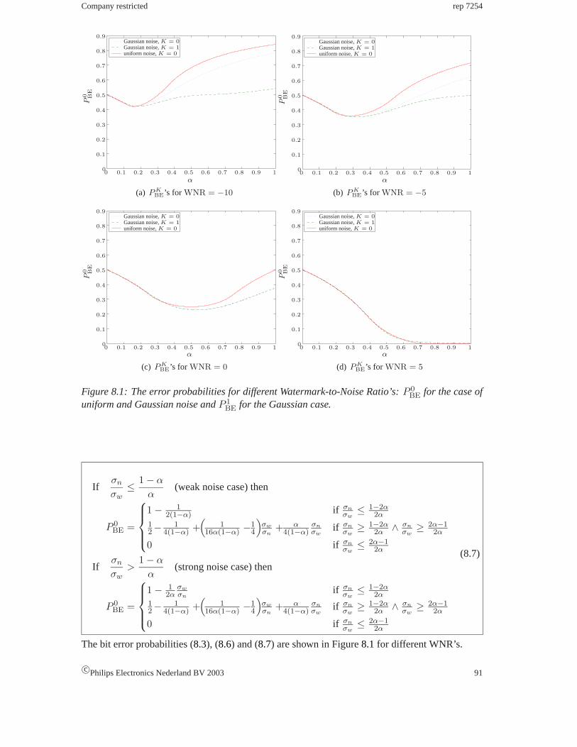
Company restricted rep 7254
Gaussian noise,K = 0Gaussian noise,K = 1uniform noise,K = 0
P0 BE
α
00
0.1
0.1
0.2
0.2
0.3
0.3
0.4
0.4
0.5
0.5
0.6
0.6
0.7
0.7
0.8
0.8
0.9
0.9 1
(a) P KBE’s for WNR = −10
Gaussian noise,K = 0Gaussian noise,K = 1uniform noise,K = 0
P0 BE
α
00
0.1
0.1
0.2
0.2
0.3
0.3
0.4
0.4
0.5
0.5
0.6
0.6
0.7
0.7
0.8
0.8
0.9
0.9 1
(b) P KBE’s for WNR = −5
Gaussian noise,K = 0Gaussian noise,K = 1uniform noise,K = 0
P0 BE
α
00
0.1
0.1
0.2
0.2
0.3
0.3
0.4
0.4
0.5
0.5
0.6
0.6
0.7
0.7
0.8
0.8
0.9
0.9 1
(c) P KBE’s for WNR = 0
Gaussian noise,K = 0Gaussian noise,K = 1uniform noise,K = 0
P0 BE
α
00
0.1
0.1
0.2
0.2
0.3
0.3
0.4
0.4
0.5
0.5
0.6
0.6
0.7
0.7
0.8
0.8
0.9
0.9 1
(d) P KBE’s for WNR = 5
Figure 8.1: The error probabilities for different Watermark-to-Noise Ratio’s:P 0BE for the case of
uniform and Gaussian noise andP 1BE for the Gaussian case.
Ifσn
σw≤ 1 − α
α(weak noise case) then
P 0BE =
1 − 12(1−α) if σn
σw≤ 1−2α
2α
12− 1
4(1−α) +(
116α(1−α) −1
4
)σwσn
+ α4(1−α)
σnσw
if σnσw
≥ 1−2α2α ∧ σn
σw≥ 2α−1
2α
0 if σnσw
≤ 2α−12α
Ifσn
σw>
1 − α
α(strong noise case) then
P 0BE =
1 − 12α
σwσn
if σnσw
≤ 1−2α2α
12− 1
4(1−α) +(
116α(1−α) −1
4
)σwσn
+ α4(1−α)
σnσw
if σnσw
≥ 1−2α2α ∧ σn
σw≥ 2α−1
2α
0 if σnσw
≤ 2α−12α
(8.7)
The bit error probabilities (8.3), (8.6) and (8.7) are shown in Figure8.1for different WNR’s.
c©Philips Electronics Nederland BV 2003 91

rep 7254 Company restricted
Gaussian noise,K = 0uniform noise,K = 0Eggers (SCS)Costa (ICS)
α∗
WNR
00
0.1
0.2
0.3
0.4
0.5
0.6
0.7
0.8
0.9
1
−20 −15 −10 −5 5 10 15 20
Figure 8.2: The optimal distortion compensation parameterα for Gaussian and uniform noiseattacks andK = 0. For uniform noise there is a clipping point in the figure. For WNR’s largerthan this clipping point the optimal distortion compensation parameterα∗ is the set of valuesbetween the two green dashed lines.
8.2 Bit error minimization and Eggers
Finding the optimal distortion compensation parameterα∗, concerns finding the functionα∗(
σwσn
)that minimizes (8.4). This is hard to solve analytically, but for a given value ofσw
σnthe correspond-
ing valueα∗ can easily be calculated numerically.
Eggers also optimized the distortion compensation parameter. However, where we minimized thechannel bit error probability, he maximized the channel capacityC
α∗ = arg maxα∈]0,1[
C
(α;
σw
σn
). (8.8)
Eggers found a numerical approximation of the capacity function. He optimized this functionnumerically and found a sequence ofα∗’s for a given WNR. He approximated this sequence withthe formula
α∗SCS =
√σ2
w
σ2w + 2.71σ2
n
, (8.9)
for the Scalar Costa Scheme (SCS).
A similar optimization problem can be defined for the case of uniform noise. In Figure8.2the op-timal distortion compensation parameterα∗ is plotted against the WNR for the different problemsand approaches: problem (8.5) with K = 1, the optimalα∗ for uniform noise, Eggers’ formula(Equation (8.9)) and for the Ideal Costa Scheme (ICS) found by Costa given by
α∗ICS =
σ2w
σ2w + σ2
n
. (8.10)
We see that our model forK = 0 is almost equal to the result of Eggers. ForK = 1 we alsoderived the optimalα∗. This improved bit error probability is plotted in Figure8.3.
92 c©Philips Electronics Nederland BV 2003

Company restricted rep 7254
Gaussian noise,K = 1Eggers (SCS)Costa (ICS)
α∗
WNR
00
0.1
0.2
0.3
0.4
0.5
0.6
0.7
0.8
0.9
1
−20 −15 −10 −5 5 10 15 20
Figure 8.3: Optimal distortion compensation parameter for the improved model (K = 1).
The improvement forK = 1 is very small, but still it is even closer to Eggers’ function than ourearlier result withK = 0. Because of the small difference between the models forK = 0 andK = 1, see Figure8.4, an increase in the value ofK is not expected to improve the estimate forthe optimal distortion compensation parameterα∗.
In order to determine the bit error probability in the presence of relatively strong noise, i.e., lowWNR’s, it is necessary to use higher values ofK. This can be seen from Figure8.1, where forlow WNR’s there is difference betweenP 0
BE andP 1BE. This is explained from the fact that for
strong noise, more quantization bins need to be taken into account. This is also why higher biterror probabilities are seen than0.5. It is also seen from Figure8.1 that for higher WNR’s, fromWNR = 0, P 0
BE andP 1BE are practically indifferent.
c©Philips Electronics Nederland BV 2003 93

rep 7254 Company restricted
Gaussian noise,K = 0Gaussian noise,K = 1
α∗
WNR
00
0.1
0.2
0.3
0.4
0.5
0.6
0.7
0.8
0.9
1
−20 −15 −10 −5 5 10 15 20
Figure 8.4: Optimal distortion compensation parameter for the two models (K = 0 andK = 1)of Gaussian noise.
94 c©Philips Electronics Nederland BV 2003
Chapter 9
Contributions, Conclusions andRecommendations
9.1 Contributions
During the internship we have done the following:
• A literature study of the state of the art of quantization watermarking was made. Anoverview of watermarking in general and quantization based watermarking is given in Chap-ter2 and3, respectively;
• The SCS is implemented in Matlab and C++;
• Two improvements of this scheme are developed: the use of error correcting codes and theuse of an adaptive quantization step size. The aim of the improvements is to get a betterrobustness of the watermarking algorithm at an equal perceptibility level of the watermark;
• Several possibilities of the adaptive quantization method are implemented in C++;
• A convolutional encoder and a corresponding Viterbi decoder are implemented in C++. Thisimplementation uses an arbitrary number of inputs and outputs, so any rate is achievable.Decoding has a high complexity, therefore it is only possible to use a memory size up toM = 9;
• A complete watermarking embedder and detector of SCS with the two improvements isimplemented in C++;
• Two models for estimating the performance of the watermarking algorithm are developed.This results in two bit error probabilitiesPBE andP∆;
• A detection thresholdT is calculated;
• The distortion compensation parameterα is optimized for a Gaussian host signal and anAWGN communication channel. This optimalα∗ is compared with a similar result of Eg-gers and is found to be equal;
• Experiments are done in order to estimate the result of the improvements.
95
rep 7254 Company restricted
9.2 Conclusions
As stated in Chapter4 we are seeking an increased robustness against AWGN and JPEG attacksand against brightness scaling. The methods we have used were Error Correcting Codes andadaptive quantization.
From Chapter5 we conclude that ECC are a valuable tool in order to decrease the bit error prob-ability and in this way increase robustness against all sorts of attacks. Concatenation of convolu-tional codes and repetition codes is valuable as long as the noise introduced by the channel is lowenough. Beyond a certain noise strength CC do not add significant robustness improvements.
Adaptive quantization strongly adds to robustness against brightness scaling; It is much better thanfixed quantization. Against AWGN the improvement from adaptive quantization is limited and forJPEG it is slightly better to use fixed quantization.
Another goal of this report is to give an analytical model for the performance of the watermarkmodel. This was done in Chapter7. The performance is measured by the bit error probability. Thebit error probability for the case of fixed quantization, distortion compensation and a uniform orGaussian noise channel is determined. This bit error probabilityPBE is a function of the distortioncompensation parameterα and the WNR. Also the bit error probability for adaptive quantization,without distortion compensation and without a noise attack is determined. The expectation ofthis bit error probabilityP∆ is a function of the mean and variance of the host signalx, and thetwo parameters in order to be able to determine the adaptive quantization step size, namelyγ andL. The developed models can be used to measure the effects of attacks and the use of adaptivequantization on robustness.
For the case of a fixed quantization step size, distortion compensation and an AWGN channelthe optimal distortion compensation parameterα∗ is determined. Using this parameter at theembedder, robustness in an AWGN situation is maximized. Theα∗ we found was compared withvalues found by Eggers [17], and was found to be identical.
If the maximum allowed distortion from the watermarkw is known i.e., ifσ2w andγ are known,
and if it is known in which range the attack strength is, i.e.,σ2n is known, then the WNR can be
calculated. For this WNR the optimal distortion compensation parameterα∗ can be derived fromChapter8. From Chapter6 we have thatL = 11 is a reasonable value to setL to. For a given host,the two derived bit error probabilities can be calculated, giving a measure of the performance inthis situation.
9.3 Recommendations
The following topics deserve to be subject of further study:
• PBE(α) can be compared with values found by experiment, using the software that wasdeveloped during the internship.
• The bit error probability for the case of adaptive quantization, with distortion compensation,and with a noise attack has to be determined in order to get a reliable measure for the overallperformance of the watermarking model. Is there a relationship between the two derived biterror probabilities and the overall one? Maybe it is possible to prove thatPtotal ≤ PBE+P∆.
• Are there other improvements, besides the use of ECC and adaptive quantization?
96 c©Philips Electronics Nederland BV 2003

Company restricted rep 7254
• The present watermarking algorithm is not robust against synchronization and geometricalattacks. Countermeasures have to be sought.
c©Philips Electronics Nederland BV 2003 97

rep 7254 Company restricted
98 c©Philips Electronics Nederland BV 2003
Appendix A
Notation
Variables and Functions
x host signaly watermarked signalyM watermarked signal, watermarked using a watermarking scheme Mw watermarkw � y − xn processing on a channel, usually considered as noiser signal received at the detection pointm messagel message lengthmc encoded messagelc encoded message lengthm message estimated at the detectork key sequenced dither sequenceα distortion compensation parameterγ embedding strength parameter∆ quantization step sizeL number of samples in an environmentN length of signalsx, y, w, n, r, dT threshold settingPBE bit error probability due to a noise attackPK
BE Kth order approximation ofPBE
P∆ bit error probability due to the estimation of∆ at the detectorerf(z) error functionerfc(z) complementary error functionQ∆(z) quantizer with step size∆�·� rounding to the nearest integer
99

rep 7254 Company restricted
Abbreviations and Acronyms
AWGN Additive White Gaussian NoiseBER Bit Error RateBMP BitMaPCC Convolutional CodeDC-QIM Distortion Compensated Quantization Index ModulationDCT Discrete Cosine TransformDFT Discrete Fourier TransformDM Dither ModulationDS-CDMA Direct Sequence Code Division Multiple AccessDVD Digital Versatile DiscDWT Discrete Wavelet TransformECC Error Correcting CodeGIF Graphics Interchange FormatHAS Human Auditory SystemHVS Human Visual SystemICS Ideal Costa SchemeIH Information HidingJPEG Joint Photographic Experts GroupLSB Least Significant BitMPEG Motion Pictures Experts GroupMSE Mean Square ErrorNASA National Aeronautics and Space Administrationpdf probability density functionSCS Scalar Costa SchemeSNR Signal-to-Noise RatioSS Spread SpectrumQIM Quantization Index ModulationWNR Watermark-to-Noise Ratio
100 c©Philips Electronics Nederland BV 2003

Appendix B
Images
(a) lena.bmp (b) baboon.bmp
(c) peppers.bmp (d) tulips.bmp
Figure B.1: The images used for experiments.
101

rep 7254 Company restricted
102 c©Philips Electronics Nederland BV 2003

Appendix C
Graphs for P∆
We have plotted the bit error probabilityP∆ due to the estimation of∆ at the detector, as a functionof ∆ and the absolute errorε1 = ∆ − ∆, see FigureC.1 andC.2. In FigureC.1∆ is plotted for0 ≤ ∆ ≤ 1 after scaling of the parameters, see Section7.3. For large values ofDelta, thedistortion becomes too high. Therefore, those large values are disregarded. Therefore, the relevantrange for∆ is more like0 ≤ ∆ ≤ 0.1 after scaling of the parameters, which is 0 to 25 beforescaling. See FigureC.2for a plot ofP∆ in this range.
103

rep 7254 Company restricted
∆
ε1000
0.10.1
0.2
0.20.2
0.3
0.4
0.4
0.5
0.6
0.6
0.8
1
−0.1−0.2
(a)
ε100 0.1
0.1
0.2
0.2
0.3
0.4
0.5
0.6
−0.1−0.2
(b)
∆
ε100 0.1
0.2
0.2
0.4
0.6
0.8
1
−0.1−0.2
(c)
∆
ε1000
0.1
0.1
0.2
0.2
0.20.3
0.4
0.40.5
0.6
0.6
0.8
1
−0.1
−0.2
(d)
Figure C.1: The bit error rateP∆ as a function of∆ andε1. P∆ is shown from different angles.∆ is in the range[0, 1].
104 c©Philips Electronics Nederland BV 2003

Company restricted rep 7254
∆
ε1000
0.1
0.10.1 0.2
0.2
0.3
0.4
0.5
0.6
−0.1−0.2 0.02
0.04
0.06
0.08
(a)
ε100 0.1
0.1
0.2
0.2
0.3
0.4
0.5
0.6
−0.1−0.2
(b)
∆
ε100
0.1
0.1 0.2−0.1−0.2
0.02
0.04
0.06
0.08
(c)
∆
ε1
000
0.1
0.1
0.2
0.20.40.6
−0.1
−0.2 0.02
0.04
0.06
0.08
(d)
Figure C.2: The bit error rateP∆ as a function of∆ andε1. P∆ is shown from different angles.∆ is in the range[0, 0.1].
c©Philips Electronics Nederland BV 2003 105

rep 7254 Company restricted
106 c©Philips Electronics Nederland BV 2003
Bibliography
[1] T.M. Apostol,Mathematical Analysis, Addison-Wesley series in Mathematics, Addison-Wesley, Reading, Massachusetts, USA, 1974.
[2] S. Baudry, Jean-Franc¸ois Delaigle, B. Sankur et al., ”Analysis of error correction strate-gies for typical communication channels in watermarking,”Signal Processing, vol. 81,no. 6, pp. 1239 - 1250, June 2001.
[3] B. Chen and G.W. Wornell, ”Digital Watermarking and Information Embedding usingDither Modulation,”Proc. of IEEE Workshop on Multimedia Signal Processing, pp. 273-278, Redondo Beach, CA, USA, December 1998.
[4] B. Chen and G.W. Wornell, ”Dither modulation: a new approach to digital watermarkingand information embedding,”Proc. of SPIE Vol. 3657: Security and Watermarking ofMultimedia Contents, pp. 342 - 353, San Jose, Ca, USA, January 1999.
[5] B. Chen and G.W. Wornell, ”An information-theoretic approach to the design of robustdigital watermarking systems”,Proc. of the IEEE International Conference on Acoustics,Speech and Signal Processing 1999 (ICASSP ’99), vol. 4, pp. 2061 - 2064, Phoenix,USA, March 1999.
[6] B. Chen and G. W. Wornell, ” Achievable performance of digital watermarking systems,”Proc. of IEEE International Conference on Multimedia Computing and Systems 1999 (ICMCS-99), Special Session on Security and Watermarking, vol. 1, pp. 13 - 18, Florence,Italy, June 1999.
[7] B. Chen and G.W. Wornell, ”Preprocessed and postprocessed quantization index modu-lation methods for digital watermarking,”Proc. of SPIE Vol. 3971: Security and Water-marking of Multimedia Contents II, pp. 48 - 59, San Jose, Ca, USA, January 2000.
[8] B. Chen, ”Design and Analysis of Digital Watermarking, Information Embedding, andData Hiding Systems,” PhD. thesis, Department of Electrical Engineering and ComputerScience, MIT, Boston, MA, USA, June 2000.
[9] B. Chen and G. Wornell, ”Quantization Index Modulation: A Class of Provably GoodMethods for Digital Watermarking and Information Embedding,”IEEE Transactions onInformation Theory, vol. 47, no. 4, May 2001.
[10] L. Chiang,Human Visual System: Visually Lossless Image Compression, [Online] Avail-able: http://www.image.ee.cityu.edu.hk/∼loben/thesis/node30.html, Accessed: 16 September 2002.
107
rep 7254 Company restricted
[11] M.H.M. Costa, ”Writing on Dirty Paper,”IEEE Transactions on Information Theory,vol. 29, no. 3, pp. 439 - 441, May 1983.
[12] T.M. Cover and J.A. Thomas,Elements of Information Theory, Wiley Series in Telecom-munications, John Wiley & Sons, New York, USA, June 1991.
[13] I.J. Cox, M. Miller, J.P.M.G. Linnartz and A.C.C. Kalker, ”A review of watermarkingprinciples and practices”, Chapter 17 ofDigital Signal Processing for Multimedia Sys-tems, pp. 461 - 486, K.K. Parhi and T. Nishitani (eds.), Marcel Dekker, Inc., New York,March 1999.
[14] I.J. Cox, M.L. Miller and J.A. Bloom, ”Digital Watermarking,” Morgan Kaufmann Pub-lishers, Inc., San Francisco, The Morgan Kaufmann Series in Multimedia and Informa-tion Science, Edward Fox (Ed.), 2001.
[15] J.J. Eggers, J.K. Su and B. Girod, ”A Blind Watermarking Scheme Based on StructuredCodebooks,”Secure Images and Image Authentication, Proc. IEE Colloquium, pp. 4/1 -4/6, London, UK, April 2000.
[16] J.J. Eggers, J.K. Su and B. Girod, ”Robustness of a blind image watermarking scheme,”Proc. of the IEEE Intl. Conference on Image Processing 2000, Vancouver, Canada,September 2000.
[17] J.J. Eggers, R. Bauml, R. Tzschoppe and B. Girod, ”Scalar Costa Scheme for Informa-tion Embedding,” submitted toIEEE Transactions on Signal Processing, 2002.
[18] J.J. Eggers and B. Girod,Informed Watermarking, The Kluwer international series in en-gineering and computer science 685, Kluwer Academic Publishers, Boston, April 2002.
[19] W. Feller,An Introduction to Probability Theory and Its Applications, Volume II, WileySeries in Probability and Mathematical Statistics, R.A. Bradley et al. (eds), John Wiley& Sons, New York, USA, 1971.
[20] R.M. Gray and T.G. Stockham, ”Dithered quantizers”,IEEE Transactions on Informa-tion Theory, vol. 39, no. 3, pp. 805 - 812, May 1993.
[21] A. Kerckhoffs, ”La cryptographie militaire,”Journal des Sciences Militaires, vol. 9, pp.5 - 38, January 1883.
[22] G.C. Langelaar, I. Setyawan and R.L. Lagendijk, ”Watermarking Digital Image andVideo Data: A State-of-the-Art Overview,”IEEE Signal Processing Magazine, vol. 17,no. 5, pp. 20 - 46, September 2000.
[23] S. Lin and D.J. Costello, ”Error Control Coding: Fundamentals and Applications”,Prentice Hall, Englewood Cliffs, NJ, February 1983.
[24] S.P. Lipschitz, R.A. Wannamaker and J. Vanderkooy, ”Quantization and dither: A theo-retical survey,” Journal of the Audio Engineering Society, vol. 40, no. 5, pp. 355 - 375,May 1992.
[25] R.J. McEliece, ”The Theory of Information and Coding: a mathematical framework forcommunication”, vol. 3, Addison-Wesley Publishing Company, Reading, MA, Encyclo-
108 c©Philips Electronics Nederland BV 2003

Company restricted rep 7254
pedia of Mathematics and its Applications, Gian-Carlo Rota (Ed.), 1977.
[26] A.M. Mayache, T. Eude and H. Cherifi, ”A comparison of image quality models andmetrics based on human visual sensitivity,”IEEE International Conference on ImageProcessing, vol. 3, pp. 409 - 413, October 1998.
[27] S.R.M. Oliveira, M.A. Nascimento and O.R. Zaıane, ”Digital Watermarking: Its Sta-tus, Limitations and Prospects,” Technical Report, Department of Computing Science,University of Alberta, Canada, Januari 2002.
[28] V.S. Pless, W.C. Huffman and R.A. Brualdi (eds),Handbook of Coding Theory, ElsevierPublishing Company, Amsterdam, The Netherlands, October 1998.
[29] S. Schimmel, ”Motion Sensitive Video Watermarking, preliminary study”, Nat.Lab. un-classified report, 2001/824, Philips Research, Eindhoven, April 2001.
[30] S. Schimmel, ”Motion Sensitive Video Watermarking, final report”, Nat.Lab. unclassi-fied report, 2001/825, Philips Research, Eindhoven, August 2001.
[31] L. Schuchman, ”Dither signals and their effect on quantization noise,”IEEE Transac-tions on Communications Technology (COM), vol. 12, pp. 162 - 165, December 1964.
[32] I. Setyawan,Attacks on Watermarking Systems, Technical Report, Information and Com-munication Theory Group, TU Delft, 2000.
[33] C.E. Shannon, ”A mathematical theory of communication,”Bell System Technical Jour-nal, vol. 27, pp. 379 - 423 and 623 - 656, July and October 1948.
[34] C.E. Shannon, ”Channels with side information at the transmitter,”IBM J. Res. Develop.,vol. 2, pp. 289 - 293, 1958.
c©Philips Electronics Nederland BV 2003 109

rep 7254 Company restricted
110 c©Philips Electronics Nederland BV 2003

Index
Aadaptive quantization . . . . . . . . . . . . . . . . . .57anonymity . . . . . . . . . . . . . . . . . . . . . . . . . . . . .4attacks
ambiguity attack . . . . . . . . . . . . . . . . . .17collusion attack . . . . . . . . . . . . . . . . . . .16DA- & AD-conversion . . . . . . . . . . . .15embedder / detector analysis . . . . . . .16general filtering . . . . . . . . . . . . . . . . . . .15geometrical attack . . . . . . . . . . . . . . . .16lossy compression . . . . . . . . . . . . . . . .15mosaic attack . . . . . . . . . . . . . . . . . . . . .16noise addition . . . . . . . . . . . . . . . . . . . .15non-linear filtering . . . . . . . . . . . . . . . .16pixel deletion / substitution . . . . . . . .16removal attack . . . . . . . . . . . . . . . . . . . .15scramble / unscramble attack . . . . . . .16statistical averaging . . . . . . . . . . . . . . .16synchronization attack . . . . . . . . . . . . .16transcoding . . . . . . . . . . . . . . . . . . . . . . .15
Bblock codes . . . . . . . . . . . . . . . . . . . . . . . . . . .44brightness masking . . . . . . . . . . . . . . . . . . . .13brightness scaling . . . . . . . . . . . . . . . . . . . . .57brightness sensitivity . . . . . . . . . . . . . . . . . .10broadcast monitoring . . . . . . . . . . . . . . . . . . .6
Ccapacity . . . . . . . . . . . . . . . . . . . . . . . . . . . . . . .9computational cost . . . . . . . . . . . . . . . . . . . . .9concatenated codes . . . . . . . . . . . . . . . . . . . .51convolutional code . . . . . . . . . . . . . . . . . . . .44convolutional representation . . . . . . . . . . . .47copy protection . . . . . . . . . . . . . . . . . . . . . . . .6copyright protection . . . . . . . . . . . . . . . . . . . .6covert channels . . . . . . . . . . . . . . . . . . . . . . . .3
Ddata authentication . . . . . . . . . . . . . . . . . . . . .6data hiding . . . . . . . . . . . . . . . . . . . . . . . . . . . .6
decoding . . . . . . . . . . . . . . . . . . . . . . . . . . . . .43deliberate attack . . . . . . . . . . . . . . . . . . . . . . .5detecting . . . . . . . . . . . . . . . . . . . . . . . . . . . . . .4detection
blind detection . . . . . . . . . . . . . . . . . . . . .9detector . . . . . . . . . . . . . . . . . . . . . . . . . . . . . . .4digital watermarking . . . . . . . . . . . . . . . . . . .4Discrete Cosine Transform . . . . . . . . . . . . .18Discrete Fourier Transform . . . . . . . . . . . .18Distortion Compensated Quantization Index
Modulation . . . . . . . . . . . . . . .24–25distortion compensation . . . . . . . . .25, 31–32dither . . . . . . . . . . . . . . . . . . . . . . . . . . . . .29–31Document-to-Watermark Ratio . . . . . . . . .51
Eembedder . . . . . . . . . . . . . . . . . . . . . . . . . . . . .4embedding . . . . . . . . . . . . . . . . . . . . . . . . . . . .4encoding . . . . . . . . . . . . . . . . . . . . . . . . . . . . .43
Ffalse negative probability . . . . . . . . . . . . . . . .8false positive probability . . . . . . . . . . . . . . . .8feature tagging . . . . . . . . . . . . . . . . . . . . . . . . .6fingerprinting . . . . . . . . . . . . . . . . . . . . . . . . . .6Fourier-Mellin Transform . . . . . . . . . . . . . .18fragile watermark . . . . . . . . . . . . . . . . . . . . . .8frequency masking . . . . . . . . . . . . . . . . . . . .13frequency sensitivity . . . . . . . . . . . . . . .10, 11
Hhard decision decoding . . . . . . . . . . . . . . . .35host data . . . . . . . . . . . . . . . . . . . . . . . . . . . . . .4host signal . . . . . . . . . . . . . . . . . . . . . . . . . . . . .4host signal interference . . . . . . . . . . . . . . . .21Human Visual System . . . . . . . . . . . . . . . . .10
IIdeal Costa Scheme . . . . . . . . . . . . . . . .22–23imperceptibility . . . . . . . . . . . . . . . . . . . . . . . .7indexing . . . . . . . . . . . . . . . . . . . . . . . . . . . . . . .6
111

rep 7254 Company restricted
Information Hiding . . . . . . . . . . . . . . . . . . . . .3
KKerckhoffs’ principle . . . . . . . . . . . . . . . . . . .9
LLeast Significant Bit modification . . . . . . .19linear codes . . . . . . . . . . . . . . . . . . . . . . . . . .44
Mmajority vote . . . . . . . . . . . . . . . . . . . . . . . . .35masking . . . . . . . . . . . . . . . . . . . . . . . . . . . . . .11Mean Square Error . . . . . . . . . . . . . . . . . . . . .7medical safety . . . . . . . . . . . . . . . . . . . . . . . . .6memory . . . . . . . . . . . . . . . . . . . . . . . . . . . . . .44memory size . . . . . . . . . . . . . . . . . . . . . . . . . .45
Nnormal processing . . . . . . . . . . . . . . . . . . . . . .5
PPatchwork algorithm . . . . . . . . . . . . . . . . . .20payload . . . . . . . . . . . . . . . . . . . . . . . . . . . . . . .9perceptual transparency . . . . . . . . . . . . . . . . .7pooling . . . . . . . . . . . . . . . . . . . . . . . . . . . . . .13proof of ownership . . . . . . . . . . . . . . . . . . . . .6
Qquantization . . . . . . . . . . . . . . . . . . . . . . . . . .28Quantization Index Modulation . . . . .23–24quantization step size . . . . . . . . . . . . . . . . . .28
Rrate . . . . . . . . . . . . . . . . . . . . . . . . . . . . . . . . . . .9repetition coding . . . . . . . . . . . . . . . . . . . . . .43robustness . . . . . . . . . . . . . . . . . . . . . . . . . . .5, 8
SScalar Costa Scheme . . . . . . . . . . . . . . . . . .26security . . . . . . . . . . . . . . . . . . . . . . . . . . . . .6, 9shift-register encoder . . . . . . . . . . . . . . . . . .45side information at the encoder . . . . . . . . .21Signal-to-Noise Ratio . . . . . . . . . . . . . . . . . . .7soft decision decoding . . . . . . . . . . . . . . . . .36spatial sensitivity . . . . . . . . . . . . . . . . . . . . . .11Spread Spectrum watermarking . . . . . . . . .19state . . . . . . . . . . . . . . . . . . . . . . . . . . . . . . . . .45state diagram . . . . . . . . . . . . . . . . . . . . . . . . .45state representation . . . . . . . . . . . . . . . . . . . .48steganography . . . . . . . . . . . . . . . . . . . . . . . . .4
subtractive dither . . . . . . . . . . . . . . . . . . . . . .29
Ttamper proofing . . . . . . . . . . . . . . . . . . . . . . . .6temporal masking . . . . . . . . . . . . . . . . . . . . .13temporal sensitivity . . . . . . . . . . . . . . . . . . .11threshold setting . . . . . . . . . . . . . . . . . . . . . .37trellis . . . . . . . . . . . . . . . . . . . . . . . . . . . . . . . .45
VViterbi algorithm . . . . . . . . . . . . . . . . . . . . . .49
Wwatermark . . . . . . . . . . . . . . . . . . . . . . . . . . . . .4Watermark-to-Noise Ratio . . . . . . . . . . . . .23watermarked signal . . . . . . . . . . . . . . . . . . . . .4watermarking . . . . . . . . . . . . . . . . . . . . . . . . . .4watermarks
visible . . . . . . . . . . . . . . . . . . . . . . . . . . . .8Watson-metric . . . . . . . . . . . . . . . . . . . . . . . . .8Weber’s law . . . . . . . . . . . . . . . . . . . . . . . . . .10
112 c©Philips Electronics Nederland BV 2003