Second quantizationGabriel T. Landi

University of Sao PauloNovember 8, 2019

Contents1 Introduction 2

2 Single-particle states 22.1 Free particles . . . . . . . . . . . . . . . . . . . . . . . . . . . . . . 22.2 Tight-binding model . . . . . . . . . . . . . . . . . . . . . . . . . . 52.3 Aubry-Andre model . . . . . . . . . . . . . . . . . . . . . . . . . . . 9

3 Creation and annihilation operators 123.1 Bosons and Fermions . . . . . . . . . . . . . . . . . . . . . . . . . . 133.2 Transformations between creation and annihilation operators . . . . . 153.3 Non-interacting Hamiltonians in the language of second quantization . 173.4 Interacting Hamiltonians . . . . . . . . . . . . . . . . . . . . . . . . 23

4 Quadratic Hamiltonians 254.1 Recipe for diagonalizing quadratic Hamiltonians . . . . . . . . . . . 254.2 The tight-binding model revisited . . . . . . . . . . . . . . . . . . . . 274.3 Electrons and holes . . . . . . . . . . . . . . . . . . . . . . . . . . . 30

5 Field quantization 315.1 The Schrodinger field . . . . . . . . . . . . . . . . . . . . . . . . . . 315.2 The Schrodinger Lagrangian . . . . . . . . . . . . . . . . . . . . . . 34

A More on the Bosonic and Fermionic algebras 37A.1 Commutators and anti-commutators . . . . . . . . . . . . . . . . . . 37A.2 Eigenstuff of bosonic operators . . . . . . . . . . . . . . . . . . . . . 38A.3 Eigenstuff of fermionic operators . . . . . . . . . . . . . . . . . . . . 40

1

1 IntroductionSecond quantization is the name given to a set of techniques which are incredibly

powerful for dealing with systems composed by a large number of particles. It is, ina sense, a different posture towards quantum mechanics. It is still quantum mechanics,but looked at in a different way. The usual formulation of quantum mechanics in termsof the tensor product amounts to specifying in which state each particle is. If wehave 1023 particles this becomes too cumbersome. Moreover, if the particles are allindistinguishable, this doesn’t even make sense anymore because we cannot say whichparticle is in which state. All we can say is how many particles are in each state.This is called occupation number representation and is the basic idea behind secondquantization.

Second quantization is extremely powerful. We will learn in these notes to thinkabout second quantization as a language. It is a different way of seeing nature. Andthis will provide us with a very nice way of unifying different fields of knowledge.Condensed matter, quantum optics, statistical mechanics and high energy physics, canall be cast in a similar language using second quantization. By learning this language,you will therefore be able to better navigate between these different fields.

Introducing second quantization for the first time can also be quite confusing. Tolearn it, gaining intuition is essential. If I try to teach you rigorously from the start,you will be very confused. Here I will therefore focus on an informal introduction tothe subject, which will allow us to jump right into applications and therefore gain in-tuition. If you are curious on how to put this on more rigorous grounds, I recommendFeynman’s Statistical Mechanics, chapter 7. The downside of doing an informal intro-duction is that you may be left with the feeling that second quantization is somewhatmystical. It is not. Second quantization is quantum mechanics. It is just written in adifferent way. Please remember that.

2 Single-particle statesThe basic idea behind the theory is the notion of single-particle states. That is, the

set of quantum states that can be occupied by a single particle. This is what will thenbe used as the building block for states with multiple particles.

2.1 Free particlesConsider a free particle in one dimension, with Hamiltonian

H =p2

2m(2.1)

Here and henceforth we set ~ = 1. To diagonalize H it suffices to diagonalize p. Welabel the eigenvalues and eigenvectors as

p|k〉 = k|k〉. (2.2)

Our goal is to find the eigenvalues k and corresponding eigenvectors |k〉. Working inthe coordinate representation, in terms of the basis |x〉, we define wavefunctions φk(x)

2

-� -� � ��

�

�

�

�

�

��

Figure 1: Dispersion relation (2.10). The values of k are actually discrete [Eq. (2.9)] but thediscreteness is proportional to 1/L and thus becomes very fine when L is the large.The levels therefore form a quasi-continuum

as1

φk(x) = 〈x|k〉, (2.4)

so that |k〉 is expanded as

|k〉 =

∫dx |x〉〈x|k〉 =

∫dx φk(x)|x〉. (2.5)

Since [x, p] = i, one may show (as done in any quantum mechanics book) that theeigenstuff equation (2.2) in coordinate representation becomes the differential equation

− i∂xφk = kφk, (2.6)

whose solutions are plane waves φk = eikx.It is extremely convenient to assume that the system is enclosed in a box of length

L and subject to Periodic Boundary Conditions (PBC). This means that φk(x + L) =

φk(x). The eigenstates are then written as

φk(x) =eikx

√L, (2.7)

where the constant is introduced so that the functions are properly normalized

L∫0

dx |φk(x)|2 = 1. (2.8)

The allowed values of k are determined by imposing the PBC condition φk(x + L) =

φk(x). in Eq. (2.7). This leads to eikL = 1. Hence, k is allowed to take on any valuek = 2π`

L , where ` = 0,±1,±2, . . ..

1 The position kets |x〉 are a bit different because they are continuous. Orthogonality and completenessmust therefore be replaced with

〈x|x′〉 = δ(x − x′),∫

dx |x〉〈x| = 1. (2.3)

But other than that, they function pretty much like normal kets.

3

To summarize, the eigenvectors of the momentum operator in a box of size Lwith PBCs are plane waves of the form (2.7), whereas the eigenvalues are

k =2π`L, ` = 0,±1,±2, . . . . (2.9)

If you want to put ~ back, you can write the eigenvalues as ~k instead. Theeigenvalues of the free particle Hamiltonian (2.1) are then simply

Ek =k2

2m. (2.10)

Eq. (2.10) is called a dispersion relation, or energy-momentum relation. Itsays how energy scales with momentum. The eigenvalues k in Eq. (2.9) arediscrete; but their spacing is proportional to 1/L and thus becomes very finewhen L is large. As a consequence, the spectrum forms a quasi-continuum.The dispersion relation (2.10) is shown in Fig. 1.

~ = 1 and other dispersion relations

Energy is related to frequency and momentum is related to wavenumber:

E = ~ω, p = ~k. (2.11)

Thus, when ~ = 1, energy = frequency and momentum = wavenumber, so feel free touse these words interchangeably. This is all that ~ does. For instance, in electromag-netic theory we find that frequency and wavenumber are related by ω = c|k|, where c isthe speed of light. Multiplying by ~ on both sides yields

E = c|p|. (2.12)

This is also a dispersion relation, although it is dramatically different from (2.10). Wesay (2.10) is a non-relativistic dispersion relation whereas (2.12) is called a masslessdispersion.

In relativity we also find things which are somewhere in the middle:

E =

√m2c4 + p2c2 (2.13)

When pc � mc2 this yields (2.10) (up to a constant) and when pc � mc2 thisyields (2.12). In solids we also find much more exotic dispersion relations, whichstem due to the confinement of electrons in the potentials created by the atoms. Wewill see one example below in Sec. 2.2

Generalization to d dimensions

The eigenstates |k〉 (or the corresponding eigenfunctions φk) are what we call asingle-particle state. They are states which completely characterize a particle in 1D.A particle in 3D can be labeled by single-particle states of the form

|k〉 = |kx, ky, kz〉 = |kx〉 ⊗ |ky〉 ⊗ |kz〉, (2.14)

4

-� -� ���

-�

-�

�

��

Figure 2: Allowed values for the momentum (kx, ky) in 2D [c.f. Eq. (2.9)]. The energy (2.15)correspond to concentric circles in k space.

which are eigenstates of px, py and pz. Since momenta in different directions commute,each operator can be diagonalized independently. Thus, each ki will be discrete exactlylike in Eq. (2.9). In 2D this is illustrated in Fig. 2, which shows a grid of (kx, ky) values.The dispersion relation (2.10) in d dimensions simply becomes

Ek =k2

2m=

k21 + . . . + k2

d

2m. (2.15)

In 2D, for instance, this corresponds to concentric circles in k space (Fig. 2).The particle may also have internal degrees of freedom. For instance, the particle

itself may be an atom, which has internal electronic energy levels. Or, even moresimply, the particle may just be an electron which also carries spin. A set of single-particle states for a spin 1/2 free particle is therefore

|k〉 = |kx〉 ⊗ |ky〉 ⊗ |kz〉 ⊗ |σ〉, (2.16)

where σ = ±1.The important message that you should remember is that a single particle state

completely characterizes the state of a single particle. I know it sounds redundant. Butplease remember it! The set of single particle states do not have to be eigenstates ofanything. For instance, if we introduce a potential V(x) in the Hamiltonian (2.1), theφk will no longer be eigenstates. Notwithstanding, they continue to be single-particlestates. In fact, a much simpler set of single-particle states are the position eigenstates|x〉. They also form a basis and they also completely characterize a particle in 1D.

2.2 Tight-binding modelTight-binding is a simplified toy model which is absolutely lovely. Electrons in

semiconductors and metals tend to be trapped near the atomic cores. They can, how-ever, move around by tunneling to neighboring atoms. The motion is therefore a se-quential composition of tunnelings. This is what we call hopping (Fig. 3). The tight-binding provides a simplified picture of this, where the particles can only like on adiscrete set of states |n〉, with n = 1, 2, . . . ,N, which are therefore the single-particlestates. If the lattice sites are spaced by a fixed amount a (the lattice spacing), then eachsite n is associated with a position xn = an.

5

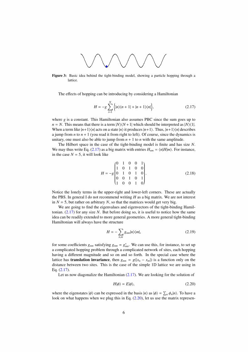
Figure 3: Basic idea behind the tight-binding model, showing a particle hopping through alattice.

The effects of hopping can be introducing by considering a Hamiltonian

H = −gN∑

i=1

{|n〉〈n + 1| + |n + 1〉〈n|

}, (2.17)

where g is a constant. This Hamiltonian also assumes PBC since the sum goes up ton = N. This means that there is a term |N〉〈N +1| which should be interpreted as |N〉〈1|.When a term like |n+1〉〈n| acts on a state |n〉 it produces |n+1〉. Thus, |n+1〉〈n| describesa jump from n to n + 1 (you read it from right to left). Of course, since the dynamics isunitary, one must also be able to jump from n + 1 to n with the same amplitude.

The Hilbert space in the case of the tight-binding model is finite and has size N.We may thus write Eq. (2.17) as a big matrix with entries Hnm = 〈n|H|m〉. For instance,in the case N = 5, it will look like

H = −g

0 1 0 0 11 0 1 0 00 1 0 1 00 0 1 0 11 0 0 1 0

. (2.18)

Notice the lonely terms in the upper-right and lower-left corners. These are actuallythe PBS. In general I do not recommend writing H as a big matrix. We are not interestin N = 5, but rather on arbitrary N, so that the matrices would get very big.

We are going to find the eigenvalues and eigenvectors of the tight-binding Hamil-tonian. (2.17) for any size N. But before doing so, it is useful to notice how the sameidea can be readily extended to more general geometries. A more general tight-bindingHamiltonian will always have the structure

H = −∑n,m

gnm|n〉〈m|, (2.19)

for some coefficients gnm satisfying gnm = g∗mn. We can use this, for instance, to set upa complicated hopping problem through a complicated network of sites, each hoppinghaving a different magnitude and so on and so forth. In the special case where thelattice has translation invariance, then gnm = g(|xn − xm|) is a function only on thedistance between two sites. This is the case of the simple 1D lattice we are using inEq. (2.17).

Let us now diagonalize the Hamiltonian (2.17). We are looking for the solution of

H|φ〉 = E|φ〉, (2.20)

where the eigenstates |φ〉 can be expressed in the basis |n〉 as |φ〉 =∑

n φn|n〉. To have alook on what happens when we plug this in Eq. (2.20), let us use the matrix represen-

6

tation in Eq. (2.18). Then

H|φ〉 = −g

φ2 + φN

φ1 + φ3

φ2 + φ4

φ3 + φ5

φ4 + φ1

= E

φ1

φ2

φ3

φ4

φ5

= E|φ〉.

We clearly see a pattern here. Each line of the above formula gives us an algebraicrelation for the coefficients φi. Moreover, we can clearly guess what is the generalform of this equation:

−g(φn−1 + φn+1) = Eφn. (2.21)

Notice how this also works for the boundary terms, provided we use the PBC recipeφN+1 = φ1. This therefore converted an eigenvalue/eigenvector problem into a recur-rence relation problem. Notice that the variables here are both the vectors φn as well asthe energies E.

The recurrence Eq. (2.21) can be solved by introducing plane waves

φkn =

eikxn

√N, (2.22)

where xn = an and k is just a label for the different plane waves. The allowed values ofk will be determined in a second. I often set the lattice spacing to be a = 1, in whichcase k becomes dimensionless. But if we keep a, then k will have units of 1/length; i.e.,wavenumber.

The normalization constant is introduced so that

N∑n=1

|φkn|

2 = 1, ∀k. (2.23)

Plugging Eq. (2.22) into Eq. (2.21) we find that

−geikn

√N

(eik + e−ik) = Eeikn

√N.

Cancelling out the exponentials, we find that the ansatz (2.22) indeed works, but onlyprovided that the energy Ek associated to the plane wave |φk〉 are given by

Ek = −2g cos ka.

This will be the dispersion relation for this model. We will analyze it in more detail ina second.

But before doing so, let us determine what are the allowed values of k. As inSec. 2.1, these are determined by imposing the PBC conditions φN+1 = φ1 in Eq. (2.22).This leads to eikaN = 1 so that k = 2π`/(Na), where ` = 0,±1,±2, . . .. Unlike the freeparticle case, however, k cannot take on an infinite number of values. The Hilbert spacein this case has dimension N, so we only need a set of N eigenvectors. What we need to

7

-π/� π/��

-��

��

Figure 4: Dispersion relation (2.26) for the tight-binding model. The values of k are actuallydiscretized as in Eq. (2.27) and restricted to the first Brillouin zone k ∈ [−π/a, π/a].

look for are the eigenvectors. The eigenvalues can be equal (that is just a degeneracy).But the eigenvectors have to be distinct to form a orthonormal basis. In (2.22) thequantities n are integers; thus, if we displace

k → k + 2π/a

we do not change φkn. As a consequence, it suffices to pick out only those values of

k which are within an interval of length 2π/a. The customary choice is a symmetricinterval

k ∈[−π

a,π

a], (2.24)

known historically as the first Brillouin zone. The correct choice for the values of kare therefore2

k =2π`Na

, −N2< ` ≤

N2.

To summarize, the eigenvectors of the tight-binding Hamiltonian (2.17) areplane waves of the form

φkn =

eikxn

√N, (2.25)

whereas the dispersion relation is

Ek = −2g cos ka. (2.26)

In both formulas, the quantum numbers k are discretrized as

k =2π`Na

, −N2< ` ≤

N2. (2.27)

where ` is an integer. This yields values of k in the first Brillouin zone k ∈[−π/a, π/a]. The dispersion relation is shown in Fig. 4.

2 Notice how I wrote < and ≤ in this expression. This is simply to ensure that we really take N distincteigenvectors. If N is odd, like N = 5, then ` can take on 5 values −2,−1, 0, 1, 2. But if N is even, like N = 6,then we cannot take −3,−2,−1, 0, 1, 2, 3. That gives 7 values. It turns out that in this case −3 and 3 give thesame eigenvector φk

n, so it suffices to choose one of them. I chose +N/2.

8

Tight-binding is kind of a free particle

The dispersion relation in Fig. 4 is, similarly to Fig. 1, not really a continuous func-tion. Rather, it is discrete in small steps of ∆k = 2π/Na. The big difference betweenthe tight-binding and free particle dispersion relations is that the latter is unbounded,with k going all the way to ±∞. In the tight-binding, on the other hand, k is restrictedto the first Brillouin zone k ∈ [−π/a, π/a].

This introduces the notions of ultra-violet and infrared cutoffs, which are nick-names we give for stuff with high and low energy respectively. The fact that the tight-binding dispersion relation is restricted to [−π/a, π/a] is an ultra-violet cutoff. And thefact that it is discrete, in steps of ∆k = 2π/Na, is an infrared cutoff. Ultraviolet isrelated to the lattice spacing a, whereas infrared is related to the total size L = Naof the chain. The free particle has the exact same infrared cutoff [Eq. (2.9)]. But noultraviolet since it has no underlying discrete lattice.

We are always interested in the limit of large chain sizes N (or large lengths L =

Na). Thus, the infrared cutoff is always vanishingly small. Sometimes we may also beinterested in the limit where the lattice spacing a is very small. In this case we mayexpand Eq. (2.26) in a, leading to

Ek ' −2g + ga2k2. (2.28)

The first term is a constant and energy is only defined up to a constant. What mattersis the second term. If we define an effective mass

me =1

2ga2 , (2.29)

we then find that

Ek 'k2

2me(2.30)

For small ka we therefore see that the tight-binding model predicts the same kind ofnon-relativistic dispersion relation as the free-particle, but with an effective mass me.In fact, from Eq. (2.29) we see that me ∝ 1/g, so that high tunneling rates make theparticles very light. This effective mass can actually be measured in semiconductorsand can vary quite dramatically, from 0.01 to 20 times the electron mass. Thus, ineffect, an electron can move through a crystal as if it were a free particle, but with acompletely different mass. Pretty cool huh?

2.3 Aubry-Andre modelLet us consider once again the tight-binding model (2.17), but introduce a lattice

dependent potential so that the Hamiltonian changes to

H =

N∑n=1

Vn|n〉〈n| − gN∑

i=1

{|n〉〈n + 1| + |n + 1〉〈n|

}, (2.31)

where Vn are arbitrary numbers. In matrix form this looks like (e.g. for N = 5):

H =

V1 −g 0 0 −g−g V2 −g 0 00 −g V3 −g 00 0 −g V4 −g−g 0 0 −g V5

. (2.32)

9

●

●

●

●

●

●●

●

●

●●

●

●

●

●

●

●

●

●

●

●

●

●

●

●

●

●●

●

●

� � �� �� �� �� ��-���

-���

���

���

���

�

���(�πη�)

Figure 5: The function cos(2πηn), where η = 12 (√

5 + 1) is the Golden Ratio, is quasi-periodicand never repeats itself.

This Hamiltonian can still be treated in pretty much the same way. For instance, if wewish to find its eigenvalues and eigenvectors, we can generalize Eq. (2.21) to read

Vnφn − g(φn−1 + φn+1) = Eφn. (2.33)

For general Vn it is quite unlikely we will be able to solve this equation analytically.But we can notwithstanding diagonalize it numerically. Just construct a big matrixlike (2.32) and find its eigenvalues and eigenvectors. The task is not too bad becausethe matrix is tridiagonal (most entries are zero).

By playing with the potential Vn one can find an incredibly rich set of behaviors.Really. You will be amazed. One particularly nice choice, first studied by Aubry andAndre, is to choose the Vn to be of the form

Vn = λ cos(2πηn), (2.34)

where λ is a constant and η = 12 (√

5 + 1) is the Golden Ratio. The reason for choosingsuch a weird potential is because it is quasi-periodic: the irrationality of η makes it sothat the Vn never repeat. The Hamiltonian (2.31) with the potential (2.34), is called theAubry-Andre model.

This model presents a localization transition. A localization transition is not aphase transition. It is a transition on the eigenvectors of the model. The transitionoccurs at λ = 1. When λ = 0 the model is just the original tight-binding Hamil-tonian (2.17), where the eigenvectors are plane waves [Eq. (2.22)]. Plane waves areextended in space; they are delocalized. We see this by analyzing |φk

n|2 as a function of

the position n. For plane waves this would be just |φkn|

2 = 1/N so all eigenvectors of thetight-binding model are completely flat in space; the probability of finding the particleis independent of the site n.

If we now start to change λ, we get some kind of spatial dependence. Since forλ , 0 the k are no longer good quantum numbers, I will use a generic index α tolabel the eigenstates. Plots for the ground-state probabilities |φ1

n|2 as a function of n

are shown in Fig. 6 for N = 100 sites and different values of λ. As can be seen, whenλ < 1 the eigenvectors are extended through all of space. Even when λ = 0.9 or 0.95,the eigenvectors are extremely spread out. But when we reach λ = 1, sorcery happens:the eigenvalues become extremely localized in a specific region of space. The amountit localizes depends on the number of sites N. For large N the localization becomessharper and sharper. Moreover, the position where it localizes is not at all obvious, butyou can tune it if you add a phase to Eq. (2.34), as Vn = λ cos(2πηn + θ). For λ > 1 theeigenvectors remain localized.

10

� �� �� �� �� ��������

�����

�����

�����

�����

�

|ϕ��

(�) λ = ���

� �� �� �� �� �������������������������������������������

�

|ϕ��

(�) λ = ���

� �� �� �� �� �������

����

����

����

����

����

�

|ϕ��

(�) λ = ���

� �� �� �� �� �������

����

����

����

����

�

|ϕ��

(�) λ = ����

� �� �� �� �� ������

���

���

���

���

���

�

|ϕ��

(�) λ = �

� �� �� �� �� ���������������������������

�

|ϕ��

(�) λ = ���

Figure 6: The ground-state wavefunction |φn|2 for the Aubry-Andre model (2.34) for different

values of λ, with g = 1 and N = 100.

Figure 7: |φαn |2 for all eigenvectors of the Aubry-Andre model for λ = 0.5 (left) and λ = 1.5(right), with g = 1 and N = 100. Here α is just an index labeling the eigenvectors.

The localization transition for the Aubry-Andre model does not occur only for theground-state. It occurs for the entire spectrum. This is shown in Fig. 7 where I plot alleigenvectors for a value of λ below and above the transition. The appearance of spotsin the graph when λ > 1 shows clearly that all eigenvectors are localized.

A more mathematical way of quantifying localization is through the Inverse Par-ticipation Ratio (IPR). For an arbitrary state |ψ〉 =

∑n ψn|n〉 the IPR is defined as

IPR(ψ) =∑

n

|ψn|4. (2.35)

When the state is completely localized the IPR will be 1 and when it is completelydelocalized [like the plane waves (2.22)] it becomes

IPR(ψ) =1

N2

N∑n=1

1 =1N.

For large sizes, this tends to zero. Thus, the IPR is a number which varies essentially

11

� �� �� �� �� ���

�����

�����

�����

�����

�����

�����

�����

�����

����������� ����� α

���

(�) λ = ���

� �� �� �� �� ������

���

���

���

���

���

����������� ����� α

���

(�) λ = ���

Figure 8: Inverse Participation Ratio (IPR) [Eq. (2.35)] for all eigenvectors of the Aubry-Andremodelfor λ = 0.5 (left) and λ = 1.5 (right), with g = 1 and N = 100.

� = ���

� = ���

� = ���

��� ��� ��� ��� ��� ��� ��� ������

���

���

���

���

���

λ

�������

Figure 9: Mean IPR as a function of λ for different values of N and g = 1.

between 0 and 1. The larger is the IPR, the more localized is a state. In Fig. 8 I plotthe IPR for the different eigenvectors of the Aubry-Andre model, below and above thetransition. The plots are quite irregular. But notice the vertical scale. It is tiny belowthe transition (extended phase) and of order 1 above it (localized phase). This becomeseven clearer if we plot the mean IPR (averaged over all eigenvectors), as shown inFig. 9. The plot clearly shows a transition occurring at λ = 1, which becomes sharperand sharper as N → ∞.

The Aubry-Andre model may at first seem simple, but it is not. Doing anything an-alytically with this model is notoriously difficult and there is much about it (and relatedmodels) which is still unknown. The Brazilian mathematician, Prof. Artur Avila, gaveseminal contributions to this field for instance, which was part of the reason he wasawarded the Fields Medal. You can read about it, for instance, in arXiv:math/0503363.

3 Creation and annihilation operatorsWe are now finally ready to introduce the idea of second quantization. In quantum

mechanics the number of particles is fixed. We may work with 1 particle. Or with 2particles. Or with 3. When say something like “consider a system of N spins”, thenumber of particles was fixed at N. The jump to second quantization is quite simple:we lift this constraint and assume that the number of particles may fluctuate. Todescribe this, we introduce creation and annihilation operators, similarly to what wedo in the case of the harmonic oscillator, but which create or annihilate actual parti-cles. This is the reason why we need single-particle states: these operators create and

12

annihilate particles in single-particle states.

Here is how it works. Let |α〉 denote an arbitrary set of orthonormal single-particle states satisfying

〈α|β〉 = δα,β. (3.1)

We then define an operator a†α and a special state |0〉, called the vacuum, suchthat

a†α|0〉 = |α〉 ≡ |1α〉. (3.2)

The operator a†α therefore creates a particle in the single-particle state |α〉. Thenotation |1α〉 is merely to emphasize that this is a state with one particle in state|α〉 . Similarly, the annihilation operator aα is designed to annihilate a particlein the state |α〉:

aα|β〉 = δα,β|0〉. (3.3)

If β , α then aα cannot annihilate and we get zero. But if β = α then aαdestroys a particle and we are back to the vacuum.

3.1 Bosons and FermionsThings become more interesting when we create multiple particles. Second quan-

tization is specifically designed to describe identical particles. In 1940 WolfgangPauli published a paper entitled “The connection between spin and statistics” wherehe shows that, as a consequence of the Lorentz group of special relativity, identical par-ticles can behave in one of two ways. Bosons are symmetric with respect to creationof two particles:

a†βa†α|0〉 = a†αa†β|0〉 := |1β, 1α〉, (3.4)

whereas Fermions are anti-symmetric:

a†βa†α|0〉 = −a†αa†β|0〉 := |1β, 1α〉. (3.5)

In the case of Bosons, due to (3.4), we can move the states around at will: |1β, 1α〉 =

|1α, 1β〉. For Fermions, however, every time we move the states around we get a minussign: |1β, 1α〉 = −|1α, 1β〉.

Pauli also showed that Bosons and Fermions have different spin values: Bosons’spins are integer valued (0,1,2,. . .) whereas Fermions’ spins are half-integers (1/2, 3/2, . . .).In the case of Fermions, in particular, if we set β = α in Eq. (3.5) we see that

(a†α)2|0〉 = −(a†α)2|0〉, (3.6)

which implies

(a†α)2 = 0 (for Fermions). (3.7)

This is the Pauli exclusion principle: it is forbidden to create two fermions on thesame single-particle state |α〉.

Eq. (3.4) implies that bosonic creation and annihilation operators should commute:

[aα, aβ] = [a†α, a†

β] = 0, (3.8)

13

whereas Eq. (3.5) implies that fermionic operators should anti-commute:

{aα, aβ} = {a†α, a†

β} = 0, (3.9)

where {A, B} = AB + BA is the anti-commutator.

In addition, one can also show that similar properties hold for the mixed com-mutation relations between aα and a†β. In the case of Bosons, we get the typicalharmonic-oscillator like commutation relations

[aα, a†

β] = δα,β. (3.10)

whereas in the case of Fermions we get the same thing, but with anti-commutators:

{aα, a†

β} = δα,β. (3.11)

These algebraic relations are the building blocks of second quantization.

Fock space for Bosons

Fock space is the generalization of Hilbert space to the case where the numberof particles is not fixed. In the case of Bosons the operators aα behave exactly likeharmonic oscillator operators (see Appendix A.2). So first there is a state |0〉 with noparticles. Then there is a set of states |α〉 ≡ |1α〉 with exactly one particle. Next thereis a set of states with two particles, which include |1β, 1α〉 as well as states of the form|2α〉. More generally, the Fock states of a Bosonic system have the form

|n1, n2, n3, . . .〉, nα = 0, 1, 2, . . . = number of particles in state |α〉.

Here I am labeling the single-particle states as α = 1, 2, 3, . . .. But, of course, you canlabel them anyway you want. For instance, if the Fock states are the position states|i〉, i = 1, 2, . . . ,N for a tight-binding lattice, then the Fock states will have the form|n1, n2, . . . , nN〉 where n42 is the number of particles in site 42. Bosons don’t satisfy thePauli exclusion principle, so we can have 20 particles on site 42, or whatever. Noticealso how in this tight-binding example, the number of single-particle states is finite(there are N of them), but the number of Fock states is infinite, since each site can haveany number of particles.

We can characterize the number of particles by defining the number operator

N =∑α

a†αaα. (3.12)

I usually don’t put hats on operators; but in this case it is useful since the letter Nappears far too often in physics! The number operator acting on the states above thenyield

N |0〉 = 0,

N |1α〉 = |1α〉,

N |1β, 1α〉 = 2|1β, 1α〉,

14

or, more generally,

N |n1, n2, n3, . . .〉 =

(∑α

nα)|n1, n2, n3, . . .〉, (3.13)

where the sum here is over all allowed single-particle states.Using the eigenvalues of N we can factor the Fock space into sectors with different

numbers of particles. We can also move from one sector to the other. This is where aαand a†α come in. Because of the commutation relations (3.10), the rules for applying aαand a†α are exactly like those of the harmonic oscillator:

a†α|n1, . . . , nα, . . .〉 =√

nα + 1 |n1, . . . , nα + 1, . . .〉, (3.14)

aα|n1, . . . , nα, . . .〉 =√

nα |n1, . . . , nα − 1, . . .〉. (3.15)

Fock space for Fermions

The situation for Fermions is almost identical. The ony difference is that Fermionssatisfy the Pauli exclusion principle (3.7). This means that we can never put more thantwo particles in the same single-particle state (see Appendix A.3). The Fock space forFermions will therefore have the form

|n1, n2, n3, . . .〉, nα = 0, 1 = number of particles in state |α〉.

Looks exactly like the bosonic case, but nα = 0, 1. Fermionic Fock states also havethe ambiguity we saw before, about which particle we create first: |1β, 1α〉 = −|1α, 1β〉.This ambiguity has no physical consequences, as long as you are consistent with yourdefinitions.

3.2 Transformations between creation and annihilation operatorsCreation operators transform like kets

Consider now two sets of single-particle states {|α〉} and {|i〉}. To each set we canattribute corresponding creation and annihilation operators aα and bi. How are thesetwo sets of operators connected? That is, how to transform from aα to bi? The bases{|α〉} and {|i〉} can be connected by a unitary transformation

|α〉 =∑

i

|i〉〈i|α〉 =∑

i

Uαi|i〉, (3.16)

where Uαi = 〈i|α〉. Now remember Eq. (3.2): the creation operators are defined by therelations

|α〉 = a†α|0〉, (3.17)

|i〉 = b†i |0〉 (3.18)

Using Eq. (3.16) we then get

a†α|0〉 = |α〉 =∑

i

Uαi|i〉 =∑

i

Uαib†

i |0〉.

15

Whence,

a†α =∑

i

〈i|α〉b†i . (3.19)

This is exactly like the transformation rule (3.16). Creation operators transform likekets! :)

Eq. (3.16) connects the two sets aα and bi by means of a unitary transformationUα,i = 〈i|α〉. A very important property of second quantization is that unitary transfor-mations preserve the algebra. Let us check this. We start with Bosons and Eq. (3.10):assume that [bi, b

†

j ] = δi j. Then

[aα, a†

β] =∑i, j

U∗αiUβ j [bi, b†

j ] =∑i, j

U∗αiUβ jδi j =∑

i

U∗αiUβi.

The resulting sum is nothing but∑i

U∗αiUβi =∑

i

Uβi(U†)iα = (UU†)β,α = δα,β,

since U is assumed to be unitary. Thus we conclude that

[bi, b†

j ] = δi j → [aα, a†

β] = δαβ. (3.20)

Unitary transformations preserve the algebra. I will leave it for you as an exerciseto show that this is also true for Fermions. Please do it. It’s almost identical as thecalculation above, but it is a good exercise.

Number operator

If we choose a basis set {|α〉} as our single-particle states, then the number operatoris N =

∑α a†αaα. But if we use a basis set {|i〉} the number operator would be N =∑

i b†i bi. Given that the number operator counts the number of particles in the system,it would be somewhat weird if N depended on our choice of basis. Indeed, it does not.We can check this using again the unitarity of the transformation (3.19):

N =∑α

a†αaα =∑α,i, j

UαiU∗α jb†

i b j.

We now carry first the sum over α, which yields a δi j. Thus

N =∑α

a†αaα =∑

i

b†i bi. (3.21)

The number operator is independent of the choice of basis.

Commutation relations

We can also use these results to establish the commutation relations between aαand bi. Again I will focus on Bosons, with the case of Fermions being identical. UsingEq. (3.19) we find

[aα, bi] =∑

j

〈 j|α〉∗[b j, b†

i ].

16

But since [b j, b†

i ] = δi j this reduces to

[aα, b†

i ] = 〈α|i〉. (3.22)

The relation for Fermions is identical, but with the anti-commutator. This result is quitenice, as it shows how to generalize the idea of creation and annihilation operators toarbitrary single-particle states (which do not necessarily form a basis).

In fact, from now on we can generalize our notations a bit and write, instead ofEqs. (3.10) and (3.11),

[aα, a†

β] = 〈α|β〉, (Bosons) (3.23)

{aα, a†

β} = 〈α|β〉, (Fermions) (3.24)

where |α〉 and |β〉 can now be arbitrary single-particle kets (not necessarily or-thogonal). If they happen to be orthogonal, we of course recover what we hadbefore. The important message conveyed by these formulas is that the amountby which aα and a†β fail to commute is related to the overlap of their single-particle wavefunctions.

3.3 Non-interacting Hamiltonians in the language of second quan-tization

So far we have only dealt with the algebraic structure of second quantization. In or-der to make this useful, we have to start expressing Hamiltonians in this new language.This turns out to be quite intuitive. Let’s work through some examples and you willsee.

Free particle

Consider the free particle in Sec. 2.1. There, we saw that a set of single-particlestates were the momentum states |k〉, where k = 2π`/L and ` = 0,±1,±2, . . .. Wemay thus work with operators ak and a†k which annihilate and create particles withmomentum k. Now consider again the single-particle Hamiltonian for the free particle:

H1 =p2

2m, (3.25)

where I am calling this H1 here just to emphasize that this is a single particle Hamil-tonian. Suppose now that we have N non-interacting free particles. The N particleHamiltonian would be

HN =

N∑i=1

p2i

2m.

But if we don’t want to specify what is the number of particles, then this expressiondoesn’t really work.

17

Second quantization approaches the problem differently (and much more ele-gantly). In second quantization the Hamiltonian of non-interacting free parti-cles is expressed as

H =∑

k

k2

2ma†kak. (3.26)

The logic behind this formula is super simple: a†kak counts how many particleshave momentum k. So we sum over all k with the energy levels k2/2m weightedby the number of particles with that k value. The Hamiltonian (3.26) does notlive in Hilbert space. It lives in Fock space; in the space where the number ofparticles is not fixed. Of course, the same logic also applies for other operators.For instance, we can define the momentum operator in second quantization as

P =∑

k

k a†kak. (3.27)

This operators quantifies the total momentum contained in the system, irre-spective of how many particles are there. Compare this also with the numberoperator:

N =∑

k

a†kak.

The idea is similar, except that in P each a†kak is weighted by k.

Non-interacting systems

Eq. (3.26) is an example of a non-interacting Hamiltonian. We can have any num-ber of particles (identical, of course), but they do not directly interact. We will learnhow to deal with interactions in a second. But before doing so, let us try to formalize abit better how to write down second-quantized versions of non-interacting Hamiltoni-ans. It turns out there is a super easy way to do this.

Consider a single-particle Hamiltonian H1 and suppose it can be diagonalizedas

H1 =∑α

εα|α〉〈α|. (3.28)

The eigenvectors |α〉 of H1 of course form a basis of single-particle states. Thus,we can define operators aα. The second-quantized version of (3.28) is thensimply

H =∑α

εα a†αaα. (3.29)

Notice the similarity in structure between (3.28) and (3.29). We essentiallyreplace |α〉〈α| with a†αaα. The logic is also the same as before: a†αaα countshow many particles are in eigenstate |α〉. The Hamiltonian is then the sum ofall possible energies εα weighted by this number of particles.

What about the situation where H1 is not diagonal? Suppose we are given a generic

18

single-particle Hamiltonian of the form

H1 =∑i, j

Hi, j|i〉〈 j|, (3.30)

where Hi, j = 〈i|H1| j〉. What to do? We first diagonalize (3.30) by introducing a unitarytransformation:

|i〉 =∑α

|α〉〈α|i〉. (3.31)

This turns (3.30) into (3.28). The corresponding second-quantized Hamiltonian is thengiven by Eq. (3.29). Now we use the transformation rule (3.19) for creation operators:

H =∑α

εαa†αaα =∑α,i, j

εα〈i|iα〉〈α| j〉a†

i a j. (3.32)

We can rearrange this as:

H =∑i, j

(∑α

〈i|α〉εα〈α| j〉)a†i a j.

The thing inside parenthesis is∑α

〈i|α〉εα〈α| j〉 = 〈i|H1| j〉 = Hi j,

which are coefficients in Eq. (3.30). Thus, we can write (3.32) as

H =∑i, j

Hi ja†

i a j.

To summarize, we thus have that the single-particle Hamiltonian

H1 =∑

i j

Hi j|i〉〈 j|, (3.33)

is written in the language of second-quantization as

H =∑

i j

Hi ja†

i a j. (3.34)

Again, notice the similarity: we simply have to replace kets |i〉 with a†i and〈 j| with a j. This important conclusion is also readily generalized to other op-erators. Let A1 denote any single-particle operator and {|i〉} any set of single-particle states. Then, the corresponding second-quantized version of A1 willbe

A =∑i, j

Ai ja†

i a j, Ai j = 〈i|A1| j〉, (3.35)

irrespective of whether or not A1 is diagonal in this basis.

19

-� -� ��

�

�

�

�

�

ϵ�

(�)

-� -� ��

�

�

�

�

�

ϵ�

(�)

Figure 10: Ground-state of N free particles in 1D for the case of (a) Bosons and (b) Fermions.

Ground state of a free particle system

Let us return to the free particle Hamiltonian (3.26). What is the ground-state?Well, this is a tricky question, because it depends on whether we assume the numberof particles is fixed or not. Each term in Eq. (3.26) is strictly positive, so the moreparticles we add, the higher will the energy be. If the number of particles can varythen, of course, the ground-state will be that state with zero particles.

But suppose that the number of particles is fixed at some value N. Then how toconstruct the state with the smallest possible energy? Well, here we have to distinguishbetween Bosons and Fermions. Bosons do not satisfy the exclusion principle, so wecan put as many of them as we want in the same state. In Eq. (3.26) the single-particleket with the lowest energy is that with k = 0. Thus, for the case of Bosons the ground-state will be a state where k = 0 is populated with N particles; viz.,

|Ψgs〉 =(a†0)N

√N!|0〉, (3.36)

where a†0 = a†k=0 is the creation operator at momentum k = 0 (see Fig. 10(a)). The fac-tor of

√N! is put here simply for normalization [see Appendix (A.2) and Eq. (A.12) for

more details]. The state (3.36) is roughly what happens in a Bose-Einstein condensate(which we will study later on). Bose-Einstein condensation (BEC) is not a condensa-tion in position space; it is a condensation in momentum space. What happens in theBEC is that a macroscopically large number of particles tend to settled down in thesame lowest energy state, which is precisely the state (3.36).

Next let us analyze the ground-state of the free particle system in the case ofFermions. Now there is the Pauli exclusion principle to care about. Let us assume,first, that there is no spin. Then the state k = 0 can hold only one Fermion. Once itis filled, we have no choice but to put the second particle in the next lowest energystate. In this case, remembering how the k are quantized as in Eq. (2.9), this state willbe k = ±2π/L. We then keep on going, filling out successive k states of increasing Ek

until we fill the N particles. The situation will then be like in Fig. 10(b).The largest filled value of k is called the Fermi momentum kF . It depends on the

value of N. We will learn more sophisticated methods of finding kF later on. For the1D case considered here, if we forget about the state with k = 0, then essentially eachvalue of |k| will take on two particles. So given that ∆k = 2π/L, we get In fact, in the1D case we simply have

kF =πNL. (3.37)

20

The ground-state of a Fermionic system can then be written as

|Ψgs〉 =

( ∏|k|≤kF

a†k

)|0〉. (3.38)

Spelled out in words: to construct the ground-state we create particles (by applying a†k)on all k states having |k| < kF , leaving the higher order momenta entirely empty. Thenumber of particles N is contained in kF .

The highest occupied energy is called the Fermi energy εF (everything with thename Fermi in this context refers to “highest occupied...”). Since εk = k2/2m, theFermi energy will be

εF =k2

F

2m(3.39)

The Fermi energy is not the ground-state energy. Instead, the ground-state energyis

Egs =∑|k|≤kF

k2

2m. (3.40)

Computing this sum if we have 42 particles can be annoying. But if N, as well as thelength of the box L, are both large, the sum can be converted to an integral. We willcome back to this below. For now I will leave Egs like this.

Free particles with spin

If we have spin, then the single-particle kets should be replaced with |k, σ〉, so theannihilation operators become akσ. Let us focus on the case of Fermions. And let usfirst assume that there are no magnetic fields present (nor any kinds of interactions).The Hamiltonian of the system then becomes

H =∑k,σ

k2

2ma†kσakσ. (3.41)

The sum is now over all values of k and both spin components σ = ±1. The energies,however, do not depend on the spin value, but only on k (because we did not put amagnetic field yet). To construct the fermionic ground-state, we proceed exactly asbefore. The only difference is that now each k value can take on two fermions so theFermi momentum kF will be half of what we had before The ground-state can then bebuilt as

|Ψgs〉 =

( ∏|k|≤kF ,σ

a†kσ

)|0〉. (3.42)

Next let us introduce a magnetic field. As we know, this shifts the energy levels by−hσ so that the Hamiltonian becomes

H =∑k,σ

(k2

2m− hσ

)a†kσakσ. (3.43)

The energies of the system now split into two energy bands, corresponding to σ = 1and σ = −1. To construct the ground-state we always need to remember the obvious:

21

-� -� ��

�

�

�

�

�

ϵ�σ

(�)

-� -� ��

�

�

�

�

�

ϵ�σ

(�)

Figure 11: (a) Pictorial construction of the ground-state of the Hamiltonian (3.43) for the caseof Fermions. (b) The energy bands in these kinds of problems are often representedin this form, with the band with σ = +1 plotted only for k > 0 and that with σ = −1for k < 0. This does not mean that it is not possible to have σ = +1 and k < 0. It issimply for presentation purposes.

the ground-state is the state with smallest possible energy. The situation will then besomewhat like that in Fig. 11. There will be two bands, each with a discrete set ofstates. The states are then populated starting from the bottom, so we fill some states inone band and some states in the other band.

This kind of system is often represented pictorially as in Fig. 11(b), where the bandwith σ = +1 is plotted only for k > 0 and that with σ = −1 only for k < 0. This kindof plot is meant to emphasize the population mismatch between the spin up and spindown bands: because of the magnetic field there are now more spins in one band thanthe other. We can define the magnetization operator as

M =∑k,σ

σ a†kσakσ = N+ − N−, (3.44)

whereNσ =

∑k

a†kσakσ, (3.45)

are the populations of the two bands. The magnetization operator is thus the imbalancebetween the populations of the two bands.

The tight-binding model in the language of second quantization

An example of the above results is the tight-binding model (2.17). Using the recipein Eq. (3.35), the corresponding Hamiltonian in the language of second quantization is

H = −gN∑

i=1

(a†i ai+1 + a†i+1ai

). (3.46)

I personally think that written in this way the tight-binding Hamiltonian makes evenmore sense than Eq. (2.17). In fact, it gives a quite nice interpretation for what quantumtunneling is: tunneling means you annihilate a particle at site i and then create a particleat site i + 1.

Notice also how, even thoughH is creating particles in one place and annihilatingin others, the process is such that particles cannot appear out of nowhere or go missing.In other words, the Hamiltonian (3.46) preserves the number of particles. This

22

is the nice thing about second quantization: we have a theory where the number ofparticles can fluctuate; the physical constraint that the number of particles is conservedis only implemented at the Hamiltonian. Since the Hamiltonian is the generator of thedynamics, if we start with 42 particles, as time moves on we will continue to have 42particles. This can be stated mathematically as

[H , N] = 0, (3.47)

where, in the case of the tight-binding Hamiltonian (3.35),

N =

N∑i=1

a†i ai. (3.48)

I will leave for you to check that (3.47) is indeed satisfied. In fact, it suffices to checkonly that

[N , a†i a j] = 0, ∀i, j. (3.49)

I will leave this for you as an exercise.

3.4 Interacting HamiltoniansBose-Hubbard model

We have seen that single-particle Hamiltonians H1 lead to second-quantized Hamil-tonians which are quadratic in creation and annihilation operators. Quadratic Hamilto-nians are thus a synonym with non-interacting systems. Interactions, on the other hand,are represented by Hamiltonians which are cubic or quartic. To illustrate the idea, let usconsider a specific model called the Bose-Hubbard model. It is a tight-binding modelfor bosons, with interactions. The Hamiltonian is written as

H = −g∑〈i, j〉

(a†i a j + a†jai) +U2

∑i

a†i a†i aiai. (3.50)

The first term is just tight-binding, which I slightly generalized to an arbitrary latticeby including a sum over nearest neighbors 〈i, j〉. The new thing is the last term. Itdescribes a type of contact interaction. It is an “interaction” because it is quartic andit is “contact” because it acts on the same site.

To understand the logic behind this term, we use the bosonic algebra a†i ai = aia†

i −1to write

a†i a†i aiai = a†i (aia†

i − 1)ai = a†i aia†

i ai − a†i ai.

We see here the appearance of the number operator ni = a†i ai:

a†i a†i aiai = ni(ni − 1). (3.51)

The interaction term therefore depends on the number of particles in each site. Intable 1 I present a little table with the values of the energy U

2 n(n − 1) for differentvalues of n. We see that if there are 0 or 1 particles, the interaction term is zero. Thisis good. It means that there is no self-interaction. The last term in (3.50) only begins

23

Table 1: Interaction energies appearing in the Bose-Hubbard model (3.50).

n 0 1 2 3 4 5

U2 n(n − 1) 0 0 U 3U 6U 10U

to contribute when there are 2 or more particles. In fact, n(n − 1)/2 is precisely thenumber of ways for n particles to interact in pairs:(

n2

)=

n!2!(n − 2)!

=n(n − 1)

2.

The Bose-Hubbard model is an important model in physics. It cannot be solvedanalytically, but there are tons of approximations which work quite well. Decadesago this model was just a theoretical exercise. But today it can be implemented inultra-cold atoms in optical lattices,3 thus making them one of the most interestingmany-body models nowadays in physics.

Fermi-Hubbard model

More important than the Bose-Hubbard model is it’s fermionic cousin, the Fermi-Hubbard model. It is again defined as a tight-binding lattice, but with an interaction ofthe form:

H = −g∑〈i, j〉,σ

(a†iσa jσ + a†jσaiσ) + U∑

i

ni,↑ni,↓. (3.52)

Here I am using the notation σ =↑, ↓ instead of σ = ±1, simply because this is howpeople usually write it. The logic behind this Hamiltonian is the following. SinceFermions satisfy the exclusion principle, we cannot have an interaction term like thatof Eq. (3.50) because we cannot put two Fermions in the same state. What we cando, however, is put two Fermions in the same site, provided they have opposite spins.The interaction term is therefore dependent on ni,↑ni,↓ which will only give a non-zerocontribution if both states (i, ↑) and (i, ↓) are filled.

It is widely believed that the Fermi-Hubbard model is capable of explaining thehigh temperature Cuprate superconductors that were discovered in the 80s. Solving thismodel would therefore explain what is, today, one of the most important unexplainedphenomena in physics: while standard superconductivity can be explained by the so-called BCS theory, high-temperature superconductivity simply cannot. Explaining itcould provide a guideline for devising superconductors at ambient temperature, whichcould revolutionize tons of applications. Needless to say, this model has no analyticalsolution. If you ever find it, book a plane ticket to Stockholm.

Electron-photon interactions

The Bose-Hubbard and Fermi-Hubbard Hamiltonians in Eqs. (3.50) and (3.52) con-tain an equal number of creation and annihilation operators. Consequently, they pre-

3 See, for instance, M. Greiner, O. Mandel, T. Esslinger, T. W. Hansch and I. Bloch, “Quantum phasetransition from a superfluid to a Mott insulator in a gas of ultracold atoms”. Nature, 415 39–44 (2002).

24

serve particle number. This is good because the particles here are electrons or atoms, sothey cannot be destroyed or created out of nothing. Other particles, however, can. Oneexample are the photons. Photonic Hamiltonians don’t need to have the same numberof creation and annihilation operators. If you shine light on a metal, for instance, theelectrons may absorb the photon and gain some energy. Or they may emit a photon andslow down a bit.

Let ck denote the fermionic annihilation operators for electrons and ak the bosonicoperators for the photons. The processes we just described can then be described bythe following Hamiltonian

H =∑k,q

Mkq

(c†k+qckaq + c†kck+qa†q

). (3.53)

The logic is the following: a term like c†k+qckaq means that we annihilate a photon withmomentum q to change the momentum of the electron from k to k + q. Of course,in second quantization we do that by first annihilating the electron with ak and thenrecreating it with a†k+q. The other term in Eq. (3.53) is, of course, just the adjoint of thefirst to make the Hamiltonian Hermitian.

The thing you should notice in the Hamiltonian (3.53) is that the number of elec-trons is conserved (as it should) but the number of photons is not. The physics of whichparticle should be conserved and which should not should thus always be encoded inthe Hamiltonian.

4 Quadratic Hamiltonians

4.1 Recipe for diagonalizing quadratic HamiltoniansAny Hamiltonian of the form (3.34), which is at most quadratic in creation and

annihilation operators, represents non-interacting systems. As we will see below,interactions involve terms with 3 or more operators. Quadratic Hamiltonians can bereadily diagonalized. In fact, we just saw how to do this by accident in the previoussection. The goal of this section is to make these ideas clearer. In fact, we will develop ageneral recipe for diagonalizing these kinds of Hamiltonians which is extremely useful.The procedure is identical for Fermions and Bosons.

Suppose we start with a generic Hamiltonian of the form (3.34). Our goal is to putit in the form of Eq. (3.29). The first thing we need to do is to diagonalize the matrixof coefficients Hi j, which means going from Eq. (3.33) to Eq. (3.30). We do that byintroducing the basis transformation (3.31), from a set of states |i〉 to a set of states |α〉which diagonalize H (from now on I will write H instead of H1 to denote the single-particle Hamiltonian). This is equivalent to introducing a diagonal representation ofthe form

H = UEU†, or Hi j =∑α

UiαεαU∗jα

where Uiα = 〈i|α〉 is the basis transformation matrix and E = diag(εα) is a diagonalmatrix with the eigenenergies εα. Since Uiα = 〈i|α〉, the matrix U is a matrix whosecolumns contain the eigenvectors |α〉.

Inserting this transformation in Eq. (3.34) we get

H =∑i, j,α

UiαεαU∗jαa†i a j.

25

We now regroup this sum as follows:

H =∑α

εα

(∑i

Uiαa†i

)(∑− jU∗jαa j

).

This motivates us to introduce a new set of operators

b†α =∑

i

Uiαa†i .

Remember: creation operators transform like kets. Since Uiα are unitary, the inversetransformation is simply:

a†i =∑α

U∗iαb†α.

With this the Hamiltonian becomes

H =∑α

εαb†αbα.

which is what we set out to do.

Let me summarize this procedure: suppose we start with a 2nd-quantized Hamil-tonian of the form

H =∑

i j

Hi ja†

i a j, (4.1)

To diagonalize it, we first diagonalize the single-particle Hamiltonian H:

H = UEU†, or Hi j =∑α

UiαεαU∗jα (4.2)

From this, introduce a new set of operators according to

b†α =∑

i

Uiαa†i , a†i =∑α

U∗iαb†α. (4.3)

Since Uiα is unitary, this preserves the algebra. Inserting these transformations,the Hamiltonian (4.1) becomes

H =∑α

εαb†αbα. (4.4)

You may also wonder: why writing (4.1) in the form (4.4) means we diagonalizedthe Hamiltonian? We diagonalized it because now the Hamiltonian (4.4) is written asa sum of independent number operators b†αbα. We therefore know how to construct thecorresponding Fock space. The eigenvalues ofH , for instance, will be of the form

E(n) =∑α

εαnα (4.5)

where nα = 0, 1 for Fermions or nα = 0, 1, 2, . . . for Bosons.

26

4.2 The tight-binding model revisitedLet us now apply this to the tight-binding model (3.46):

H = −gN∑

i=1

(a†i ai+1 + a†i+1ai

).

The matrix H in this case is this case is the same as we studied in Sec. 2.2; e.g.,Eq. (2.18):

H = −g

0 1 0 0 11 0 1 0 00 1 0 1 00 0 1 0 11 0 0 1 0

.To diagonalize H we therefore first need to import all we learned from Sec. 2.2 aboutthe single-particle tight-binding model. As we have seen, H is diagonalized by intro-ducing a Fourier transform:

Uik =eikxi

√N, (4.6)

where xi = i with i = 1, 2, 3, . . . (I set the lattice spacing to 1 and write xi just so thatwe don’t confuse with the imaginary unit). Moreover the values of k are quantized asin Eq. (2.27):

k =2π`N, −

N2< ` ≤

N2. (4.7)

The numbers k are going to play the role here of the eigenvalue index α. In fact, theenergy eigenvalues, as we have seen, are

εk = −2g cos k. (4.8)

I will also be careful not to mix i, j with k, q. The former refer to positions, withi, j = 1, 2, . . . ,N; the latter refer to momenta, with k, q quantized as in (4.7).

Before proceeding, let us verify that the matrix U in Eq. (4.6) is indeed unitary:

(U†U)k,q =∑

j

U∗jkU jq =1N

N∑j=1

ei(k−q)x j .

The resulting sum is nothing but a finite geometric series:

N∑j=1

ei(k−q)x j =

N∑j=1

eiθ j = eiθ(

eiθN − 1eiθ − 1

), (4.9)

where θ = k − q. But because of Eq. (4.7), the term in the numerator involves eiθN =

ei2π(`−`′) = 1. The sum therefore vanishes identically. The only exception is whenk = q, in which case we get ei(k−q)x j = 1 so that the sum reduces to adding N times thenumber 1. We thus conclude that, indeed

(U†U)k,q = δkq, → U†U = 1,

so that U is indeed unitary. I will leave it for you to show that UU† = 1 as well. Thisalso follows from a finite geometric series like (4.9); it is only a bit more annoyingbecause the values of k don’t range from 1, . . . ,N. But you can translate them to do so.

27

Returning now to our recipe, now that we have the diagonal structure (4.2) of H, thenext step is to introduce a new set of creation and annihilation operators as in Eq. (4.3):

bk =1√

N

∑i

eikxi ai, ai =1√

N

∑k

e−ikxk bk. (4.10)

The tight-binding Hamiltonian then becomes

H =∑

k

εkb†kbk, (4.11)

which is in diagonal form.

Dealing with k sums:

Once we have a Hamiltonian in the form (4.11), we can proceed to computephysical observables, such as the ground-state, the average energy and so on.To do so we must deal with sums over the discretized k-values (4.7). If thenumber of sites is small, these sums are difficult to handle. But if N becomeslarge, we can approximate the sums to an integral. There is a neat trick to dothis. Consider a generic sum of the form∑

k

f (k) (4.12)

where f (k) is an arbitrary function. Due to the discretization (4.7), the valuesof k are spaced by

∆k =2πN, (4.13)

which become infinitesimally small when N becomes large. We then multiplyEq. (4.12) by the convenient 1: namely 1 = N

2π∆k. This leads to∑k

f (k) =N2π

∑k

∆k f (k).

When N → ∞, or ∆k → 0, this approaches exactly the definition of a Riemannsum that we learn in Introductory Calculus. Whence, we find

∑k

f (k) =N2π

∫dk f (k) (4.14)

This is the recipe for converting sums to integrals: always multiply by the“convenient 1”. The limits of integration will be [−π, π] in the case of thetight-binding model, or −∞ to∞ in the case of free particles.

If we wish to consider spin 1/2 fermions, the result is identical. All we need to dois change the original Hamiltonian to

H = −g∑i,σ

(a†i,σai+1,σ + a†i+1,σai,σ

),

28

which now contains also a sum over σ = ±1. But since the hopping part does notdepend on σ at all, we just need to carry the index σ around everywhere. This thenleads to the diagonal Hamiltonian

H =∑k,σ

εkb†k,σbk,σ. (4.15)

Ground-state in the Fermionic case

As an application of this formula, let us find the Fermi momentum (the momentumof the highest filled state). To this end we need to distinguish between N, which is thenumber of sites, and Np, which is the number of particles in the system. We can have,for instance, N = 10 sites filled with Np = 3 particles. Let us assume for concretenessthat the Fermions have spin 1/2, so that the Hamiltonian is given by Eq. (4.15). In thiscase each site can take on at most 2 Fermions, so that Np ≤ 2N. The Fermi momentumis defined implicitly by ∑

|k|<kF ,σ

= 2∑

k

θ(kF − |k|) = Np, (4.16)

where θ(x) is the Heaviside function: θ(x) = 1 if x > 0 and θ(x) = 0 if x < 0. In words,this formula means means that kF is the value of k which is such that, if you sum up tokF you get Np particles. Converting this to an integral we find

2N2π

π∫−π

dkθ(kF − |k|) = Np.

We can also write this as

N2π

4

kF∫0

dk =Nπ

kF = Np,

which leads tokF = πNp/N :=

π

2np. (4.17)

The Fermi momentum depends on the particle density np ∈ [0, 2].The dispersion relation (4.8) filled with different values of np is illustrated in Fig. 12.

It is customary to use as reference the case of half-filling, where Np = N so np = 1.When the system is at half-filling, we fill exactly half of the band. The Fermi energy is

εF = −2g cos kF = −2g cos(πnp/2

), (4.18)

which therefore depends non-linearly on np.Let us also compute the ground-state energy. It is defined as

Egs =∑|k|<kF ,σ

εk (4.19)

Transforming the sum to an integral and using the fact that εk = −2g cos k is an evenfunction of k, we get

Egs = −g4Nπ

kF∫0

dk cos k.

29

-π -π/� π/� π�

-�

-�

�

�

ϵ�/�(�)

-π -π/� π/� π�

-�

-�

�

�

ϵ�/�(�)

-π -π/� π/� π�

-�

-�

�

�

ϵ�/�(�)

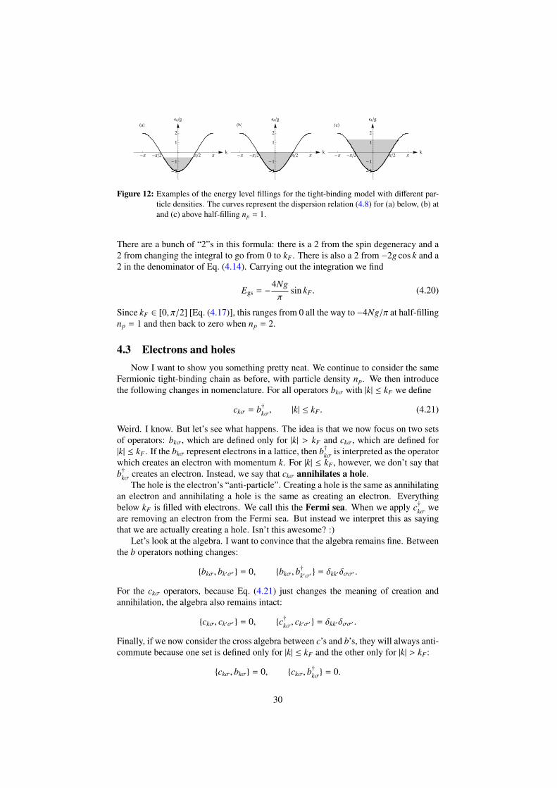
Figure 12: Examples of the energy level fillings for the tight-binding model with different par-ticle densities. The curves represent the dispersion relation (4.8) for (a) below, (b) atand (c) above half-filling np = 1.

There are a bunch of “2”s in this formula: there is a 2 from the spin degeneracy and a2 from changing the integral to go from 0 to kF . There is also a 2 from −2g cos k and a2 in the denominator of Eq. (4.14). Carrying out the integration we find

Egs = −4Ngπ

sin kF . (4.20)

Since kF ∈ [0, π/2] [Eq. (4.17)], this ranges from 0 all the way to −4Ng/π at half-fillingnp = 1 and then back to zero when np = 2.

4.3 Electrons and holesNow I want to show you something pretty neat. We continue to consider the same

Fermionic tight-binding chain as before, with particle density np. We then introducethe following changes in nomenclature. For all operators bkσ with |k| ≤ kF we define

ckσ = b†kσ, |k| ≤ kF . (4.21)

Weird. I know. But let’s see what happens. The idea is that we now focus on two setsof operators: bkσ, which are defined only for |k| > kF and ckσ, which are defined for|k| ≤ kF . If the bkσ represent electrons in a lattice, then b†kσ is interpreted as the operatorwhich creates an electron with momentum k. For |k| ≤ kF , however, we don’t say thatb†kσ creates an electron. Instead, we say that ckσ annihilates a hole.

The hole is the electron’s “anti-particle”. Creating a hole is the same as annihilatingan electron and annihilating a hole is the same as creating an electron. Everythingbelow kF is filled with electrons. We call this the Fermi sea. When we apply c†kσ weare removing an electron from the Fermi sea. But instead we interpret this as sayingthat we are actually creating a hole. Isn’t this awesome? :)

Let’s look at the algebra. I want to convince that the algebra remains fine. Betweenthe b operators nothing changes:

{bkσ, bk′σ′ } = 0, {bkσ, b†

k′σ′ } = δkk′δσσ′ .

For the ckσ operators, because Eq. (4.21) just changes the meaning of creation andannihilation, the algebra also remains intact:

{ckσ, ck′σ′ } = 0, {c†kσ, ck′σ′ } = δkk′δσσ′ .

Finally, if we now consider the cross algebra between c’s and b’s, they will always anti-commute because one set is defined only for |k| ≤ kF and the other only for |k| > kF :

{ckσ, bkσ} = 0, {ckσ, b†

kσ} = 0.

30

Next let us look at the number operator:

N =∑kσ

b†kσbkσ =∑|k|≤kF ,σ

b†kσbkσ +∑|k|>kF ,σ

b†kσbkσ.

In the first term we use Eq. (4.21) to write∑|k|≤kF ,σ

b†kσbkσ =∑|k|≤kF ,σ

ckσc†kσ =∑|k|≤kF ,σ

(1 − c†kσckσ),

where I used the fermionic algebra to write ckσc†kσ = 1 − c†kσckσ. The first term in thesum is exactly the definition of the Fermi momentum in Eq. (4.16). Hence, the numberoperator may be written as

N = Np +∑|k|>kF ,σ

b†kσbkσ −∑|k|≤kF ,σ

c†kσckσ = Np + Ne − Nh. (4.22)

The number operator is centered around Np (the actual number of particles). Electronscount positively to N , whereas holes count negatively. Holes are indeed anti-particles!We also do the same for the Hamiltonian (4.15). I will leave for you as an exercise toshow that it can be written as

H = Egs +∑|k|>kF ,σ

εkb†kσbkσ −∑|k|≤kF ,σ

εkc†kσckσ. (4.23)

Using this Fermi sea idea, we can really picture the lattice as being populated bytwo species, electrons and holes. In the tight-binding model these two species do notinteract with each other. This is visible in Eq. (4.23), where the Hamiltonian is just thesum of the Hamiltonians of the two species. But if we add additional ingredients to themodel, the two species will begin to interact.

5 Field quantization

5.1 The Schrodinger fieldThe operator a†α creates a particle at the single-particle state |α〉. Well, position is

also a single-particle state |x〉. Then why not define an operator a†x which creates aparticle at position |x〉? Yeah, we can definitely do that. Except that we don’t call it ax;we use a cooler symbol:

ax := ψ(x) = annihilation operator for a particle at position x. (5.1)

There is a neat reason as to why we use the sacred symbol ψ of wavefunctions. As wewill see, ψ(x) does behave a lot like wavefunctions. Except that it is now an operator.This is why we call this second quantization: it is a little bit like we are “quantizing”the wavefunction itself. In first quantization we quantize position and momentum. Insecond quantization, we also quantize the wavefunction. This is not very precise andthe name stuck mostly for historical reasons. But that is kind of the logic.

31

If the system has spin, we upgrade ψ with an additional internal index ψσ(x). Thiscan be σ = ±1 in the case of spin 1/2 or it can be an arbitrary spin value. The commu-tation relations of the ψσ are obtained using the general result (3.22). Since positionkets satisfy 〈x|x′〉 = δ(x − x′) we get[

ψσ(x), ψ†σ′ (x′)]

= δσ,σ′δ(x − x′), (Bosons) (5.2){ψσ(x), ψ†σ′ (x′)

}= δσ,σ′δ(x − x′). (Fermions) (5.3)

What about Hamiltonians? Consider first the case of non-interacting systems. Thetypical single-particle Hamiltonian has the form

H1 =p2

2m+ V(x), (5.4)

where V(x) is some external potential. As we learn in undergraduate quantum mechan-ics, if we move to the position representation we get

〈x|H1|φ〉 =

[−

12m

∂2x + V(x)

]〈x|φ〉,

for any wavefunction |φ〉. Choosing |φ〉 = |x′〉 we then get

〈x|H1|x′〉 = −1

2m∂2

∂x2 δ(x − x′) + V(x)δ(x − x′)

= −1

2m∂2

∂x′2δ(x − x′) + V(x)δ(x − x′), (5.5)

where, in the second line, the only thing I did was change the derivative from x to x′.This is allowed because ∂

∂xδ(x − x′) = − ∂∂x′ δ(x − x′). But when we differentiate twice,

the minus sign goes away.The general second-quantized version of the single-particle Hamiltonian (5.4) can

then be readily found from the recipe in Eq. (3.30):

H =

∫dx dx′〈x|H1|x′〉ψ†(x)ψ(x′)

=

∫dx dx′

[−

12m

∂2

∂x′2δ(x − x′) + V(x)δ(x − x′)

]ψ†(x)ψ(x′).

The term involving ∂2xδ(x − x′) is somewhat awkward. But we can get rid of it by inte-

grating by parts. In this case integrating by parts means moving a derivative from oneside to another. There are no cross terms because these are evaluated at the boundariesof the box and we use periodic boundary conditions, so any boundary terms vanish.Integrating by parts once:∫

dx dx′[∂2

∂x′2δ(x − x′)

]ψ†(x)ψ(x′) = −

∫dx dx′

[∂

∂x′δ(x − x′)

][ψ†(x)

∂

∂x′ψ(x′)

]This is the logic of integration by parts. I know this is not very rigorous, But one canarrive at the same result in a more formal way. I promise! Integrating by parts againwe get∫

dx dx′[∂2

∂x′2δ(x − x′)

]ψ†(x)ψ(x′) =

∫dx dx′δ(x − x′)

[ψ†(x)

∂2

∂x′2ψ(x′)

].

Now that the delta function is free, we can use its property to eliminate the integral inx or x′.

32

As a result, we then finally obtain

H =

∫dx ψ†(x)

[−

12m

∂2

∂x2 + V(x)]ψ(x). (5.6)

This is the second quantized version of a non-interacting Hamiltonian. It isexactly the same as the general recipe (3.30), but specialized to the case ofposition eigenkets. This introduces the peculiarity that it contains only oneintegral (which plays the role of the sum), whereas (3.30) contains two.

We can also include interactions in the same spirit. As we saw before,interactions involve more than two operators. For instance, the analog of theBose-Hubbard Hamiltonian (3.50) is

H =

∫dx ψ†(x)

[−

12m

∂2

∂x2 +V(x)]ψ(x)+

U2

∫dx ψ†(x)ψ†(x)ψ(x)ψ(x). (5.7)

This is the Hamiltonian modeling a superfluid. The term V(x) refers to anexternal potential where the particles are trapped, whereas the last term is theirCoulomb repulsion.

The free particle revisited

Consider the free particle in a box, obtained by setting V(x) = 0 in Eq. (5.6). Thesecond quantized Hamiltonian is then

H =

∫dx ψ†(x)

[−

12m

∂2

∂x2

]ψ(x). (5.8)

We now introduce a Fourier transform

ψ(x)† =1√

L

∑k

eikxa†k , k =2π`L, ` = 0,±1,±2, . . . . (5.9)

Unlike in tight-binding, here the momentum can take on an infinite number of valuesranging from −∞ to∞.

Introducing (5.9) in (5.8) we get the following:

∂2

∂x2ψ(x) =1√

L

∑k

(−ik)2e−ikxak

Thus,

H =1L

∫dx

∑k,k′

ei(k′−k)x(−ik)2a†k′ak.

Integrating over x and using

1L

∫dx ei(k′−k)x = δk,k′ , (5.10)

we finally get

H =∑

k

k2

2ma†kak, (5.11)

which is the free particle result we analyzed before.

33

5.2 The Schrodinger LagrangianIt is possible to cast Schrodinger’s equation as a consequence of the principle of

least action, similar to what we do in classical mechanics. This is fun because itformulates quantum mechanics as a classical theory, as weird as that may sound. Thisallows us to connect second quantization with field theory.

The principle of least action

Let us start with a brief review of classical mechanics. Consider a system describedby a set of generalized coordinates qi and characterized by a Lagrangian L(qi, ∂tqi). Theaction is defined as

S =

t2∫t1

L(qi, ∂tqi) dt. (5.12)

The motion of the system is then generated by the principle of least action; ie, by re-quiring that the actual path should be an extremum of S . We can find the equations ofmotion (the Euler-Lagrange equations) by performing a tiny variation in S and requir-ing that δS = 0 (which is the condition on any extremum point; maximum or mini-mum). To do that we write qi → qi + ηi, where ηi(t) is supposed to be an infinitesimaldistortion of the original trajectory. We then compute

δS = S [qi(t) + ηi(t)] − S [qi(t)]

=

t2∫t1

dt∑

i

{∂L∂qi

ηi +∂L

∂(∂tqi)∂tηi

}

=

t2∫t1

dt∑

i

{∂L∂qi− ∂t

(∂L

∂(∂tqi)

)}ηi.

where, in the last line, I integrated by parts the second term. Setting each term propor-tional to ηi to zero then gives us the Euler-Lagrange equations

∂L∂qi− ∂t

(∂L

∂(∂tqi)

)= 0. (5.13)

The example you are probably mostly familiar with is the case when

L =12

m(∂tq)2 − V(q), (5.14)

with V(q) being some potential. In this case Eq. (5.13) gives Newton’s law

m∂2t q = −

∂V∂q. (5.15)

Another example, which you may not have seen before, but which will be interestingfor us, is the case when we write L with both the position q and the momenta p asgeneralized coordinates; , ie L(q, ∂tq, p, ∂t p). For instance,

L = p∂tq − H(q, p), (5.16)

34

where H is the Hamiltonian function. In this case there will be two Euler-Lagrangeequations for the coordinates q and p:

∂L∂q− ∂t

(∂L

∂(∂tq)

)= −

∂H∂q− ∂t p = 0

∂L∂p− ∂t

(∂L

∂(∂t p)

)= ∂tq −

∂H∂p

= 0.

Rearranging, this gives us Hamilton’s equations

∂t p = −∂H∂q

, ∂tq =∂H∂p

. (5.17)

Another thing we will need is the conjugated momentum πi associated to a gen-eralized coordinate qi. It is always defined as

πi =∂L

∂(∂tqi). (5.18)

For the Lagrangian (5.14) we get π = m∂tq. For the Lagrangian (5.16) we have twovariables, q1 = q and q2 = p. The corresponding conjugated momenta are π(q) = p andπ(p) = 0 (there is no momentum associated with the momentum!). Once we have themomentum we may construct the Hamiltonian from the Lagrangian using the Legendretransform:

H =∑

i

πi∂tqi − L (5.19)

For the Lagrangian (5.14) we get

H =p2

2m+ V(q),

whereas for the Lagrangian (5.16) we get

H = π(q)∂tq + π(p)∂t p − L = p∂tq + 0 − p∂tq + H = H,

as of course expected.When we go from Lagrangian to Hamiltonian, in Eq. (5.19), we can also quantize

our theory. In terms of Lagrangians, qi are classical variables and the Lagrangian maydepend on qi and ∂tqi. When we go to a Hamiltonian formulation, we must express theHamiltonian in terms of the coordinates qk and the associated conjugated momenta πi.We then promote qi and πi to operators satisfying the canonical algebra

[qi, π j] = iδi j (5.20)

This is the idea of canonical quantization.

A principle of least action for Schrodinger’s equation

Now consider Schrodinger’s equation in first quantization

i∂tψ = Hψ, (5.21)

35

where ψ is just the usual c-number wavefunction. We can write this in terms of anarbitrary basis |n〉 by defining ψn = 〈n|ψ〉. Schrodinger’s equation then becomes

i∂tψn =∑

m

Hn,mψm, (5.22)

where Hn,m = 〈n|H|m〉. We now ask the following question: can we cook up a La-grangian and an action such that the corresponding Euler-Lagrange equations giveEq. (5.22)? The answer, of course, is yes.4 The “variables” in this case are all com-ponents ψn. But since they are complex variables, we actually have ψn and ψ∗n as anindependent set. For reasons which will become clear in a second, I will write ψ†ninstead of ψ∗n. At this level this is the same thing since ψn is just a c-number. TheLagrangian is then L = L(ψn, ∂tψn, ψ

†n, ∂tψ

†n). and the action is

S [ψ†n, ψn] =

t2∫t1

L(ψn, ∂tψn, ψ†n, ∂tψ

†n) dt. (5.23)

The correct Lagrangian we should use is

L =∑

n

iψ†n∂tψn −∑n,m

Hn,mψ†nψm. (5.24)

where ψn and ψ†n are to be interpreted as independent variables. Please take notice ofthe similarity with Eq. (5.16): ψn plays the role of q and ψ†n plays the role of p. Tocheck that this works we use the Euler-Lagrange equations for the variable ψ†n:

∂L

∂ψ†n− ∂t

(∂L

∂(∂tψ†n)

)= 0.

The second term is zero since ∂tψ†n does not appear in Eq. (5.24). The first term then

gives∂L

∂ψ†n= i∂tψn −

∑m

Hn,mψm = 0.

which is precisely Eq. (5.22). Thus, we have just cast Schrodinger’s equation as aprinciple of least action for a weird action that depends on the quantum state |ψ〉. I willleave to you as an exercise to compute the Euler-Lagrange equation for ψn; you willsimply find the complex conjugate of Eq. (5.22).

Eq. (5.24) is written in terms of the components ψn of a certain basis. We can alsowrite it in a basis independent way, as

L = 〈ψ|(i∂t − H)|ψ〉 (5.25)

This is what I call the Schrodinger Lagrangian. Isn’t it beautiful?We can also ask what is the conjugated momentum associated with the variable ψn

for the Lagrangian (5.24). Using Eq. (5.18) we get,

π(ψn) =∂L

∂(∂tψn)= iψ†n, π(ψ†n) = 0 (5.26)

4If the answer was no, I would be a completely crazy person, because I just spent more than two pagesdescribing Lagrangian mechanics, which would have all been for nothing.

36

This means that ψn and iψ†n are conjugated variables. As a sanity check, we can nowfind the Hamiltonian using the definition (5.19):

H =∑

n

iψ†n∂tψn − L =∑n,m

Hn,mψ†nψn. (5.27)

which is just the actual Hamiltonian.Finally, we can write it in terms of the coordinate representation. In this case the

action can be expressed in terms of a Lagrangian density as

S [ψ∗, ψ] =

∫dt dx L(ψ, ∂tψ, ψ

∗, ∂tψ∗), (5.28)

where

L = iψ†(x)∂tψ(x) − ψ†(x)[−

12m

∂2

∂x2 + V(x)]ψ(x). (5.29)

Written in this way, Schrodinger equation is thus seen to be a classical field theory forthe field ψ(x).

We can now quantize the Schrodinger field using the canonical quantization pro-cedure. I know this is a bit weird, but let’s see what comes out of it. The procedureis to (i) move to the Hamiltonian representation, (ii) express it in terms of coordinatesand conjugated momenta and (iii) promote them to operators satisfying the canonicalalgebra (5.20). But the momentum π conjugated to ψ(x) and ψ†(x) are, according toEq. (5.26), given by π(ψ(x)) = iψ†(x) and π(ψ†(x)) = 0. The former, when combinedwith the canonical quantization condition (5.20), implies that

[ψ(x), iψ†(x)] = iδ(x − x′), (5.30)

where I replaced the Kronecker with a Dirac delta. Notice how the factors of i cancelout, leaving us with

[ψ(x), ψ†(x)] = δ(x − x′), (5.31)

which is exactly the commutation relations for Bosons in Eq. (5.2). This is a neatway of showing why second quantization is indeed a second quantization: we interpretSchrodinger’s equation as a classical equation and then requantize it. This promotesthe wavefunction to an operator satisfying the canonical algebra (5.31). We coulddo something analogous to Fermions, by assuming that canonical quantization shouldinvolve anti-commutators. Of course, at this level, this has to be done pretty much byhand. The true origin of anti-commutation relations for Fermions can only be justifiedin quantum field theory.

A More on the Bosonic and Fermionic algebras

A.1 Commutators and anti-commutatorsThe following formulas are useful to know:

[A, BC] = B[A,C] + [A, B]C (A.1)

[AB,C] = A[B,C] + [A,C]B (A.2)

37

There is an easy way to remember them. For instance, in [A, BC] you first take B outto the left and then C out to the right.

For Fermionic operators we sometimes like to convert commutators into anti-commutators:

[A, BC] = {A, B}C − B{A,C} (A.3)

[AB,C] = A{B,C} − {A,C}B (A.4)

You can remember this as follows: the logic is the same as in Eqs. (A.1) and (A.2), butfor anti-commutators, whenever an operator need to jump over someone to escape, itgains a minus sign. For 4 operators we have

[AB,CD] = −AC{D, B} + A{C, B}D −C{D, A}B + {C, A}DB (A.5)

A.2 Eigenstuff of bosonic operatorsIn this appendix I summarize a calculation found in any quantum mechanics book:

Given a non-Hermitian operator a satisfying

[a, a†] = 1, (A.6)

what are the eigenvalues and eigenvectors of a†a. This is a really important problemthat appears often in all areas of quantum physics: given an algebra, find the eigenstuff.I think this is one of those things that everyone should go through once. So here we go.

Since a†a is Hermitian, its eigenvalues must be real and its eigenvectors can bechosen to form an orthonormal basis. Let us write them as

a†a|n〉 = n|n〉. (A.7)

Our goal is to find the allowed n and the corresponding |n〉. We of course already knowthat n is an integer. But let’s pretend we did not know and let’s figure out how thisfollows from the algebra.

The first thing we notice is that a†a must be positive semi-definite operator, so ncannot be negative:

n = 〈n|a†a|n〉 ≥ 0.

Next we use Eq. (A.6) to show that

[a†a, a] = −a, [a†a, a†] = a†. (A.8)

This type of structure is a signature of a ladder-like spectrum (that is, when the eigen-values are equally spaced). To see that, we use these commutation relations to compute:

(a†a)a|n〉 = [a(a†a) − a]|n〉 = a(a†a − 1)|n〉 = (n − 1)a|n〉. (A.9)

Hence, we conclude that if |n〉 is an eigenvector with eigenvalue n, then a|n〉 is alsoan eigenvector, but with eigenvalue (n − 1) [This is the key argument. Make sure youunderstand what this sentence means.]. However, I wouldn’t call this |n − 1〉 just yetbecause a|n〉 is not normalized. Thus we need to write

|n − 1〉 = γa|n〉,

where γ is a normalization constant. To find it we simply write

1 = 〈n − 1|n − 1〉 = |γ|2〈n|a†a|n〉 = |γ|2n.

38

Thus |γ|2| = 1/n. The phase of γ is arbitrary so we choose it for simplicity as being realand positive. We then get

|n − 1〉 =a√

n|n〉.

From this analysis we conclude that a reduces the eigenvalues by unity:

a|n〉 =√

n|n − 1〉.

We can do a similar analysis with a†. We again use Eq. (A.8) to compute

(a†a)a†|n〉 = (n + 1)a†|n〉.

Thus a† raises the eigenvalue by unity. The normalization factor is found by a similarprocedure: we write |n + 1〉 = βa†|n〉, for some constant β, and then compute

1 = 〈n + 1|n + 1〉 = |β|2〈n|aa†|n〉 = |β|2〈n|(1 + a†a)|n〉 = |β|2(n + 1).

Thusa†|n〉 =

√n + 1|n + 1〉.

Now comes the trickiest (and most beautiful) argument. We have seen that if n isan eigenvalue, then n± 1, n± 2, etc., will all be eigenvalues. But this doesn’t mean thatn itself should be an integer. Maybe we find one eigenvalue which is 42.3; then 41.3,43.3 and so on will also be eigenvalues. But suppose we start with some eigenstate|n〉 and keep on applying a a bunch of times. At each application we will lower theeigenvalue by one tick:

a` |n〉 =√

n(n − 1) . . . (n − ` + 1)|n − `〉.

But this party cannot continue forever because, as we have just discussed, the eigen-values of a†a cannot be negative. They can, at most, be zero. The only way for this tohappen is if there exists a certain integer ` for which a` |n〉 , 0 but a`+1|n〉 = 0. Andthis can only happen if ` = n because, then

a`+1|n〉 =√

n(n − 1) . . . (n − ` + 1)(n − `)|n − ` − 1〉 = 0,

and the term n − ` will vanish. Since ` is an integer, we therefore conclude that n mustalso be an integer. Thus, we finally conclude that

eigs(a†a) = n ∈ {0, 1, 2, 3, . . .}. (A.10)

It is for this reason that a†a is called the number operator: we usually say a†a counts thenumber of quanta in a given state: given a state |n〉, you first apply a to annihilate onequant and then a† to create it back again. The proportionality factor is the eigenvaluen. Curiously, this analysis seem to imply that if you want to count how many peoplethere are in a room, you first need to annihilate one person and then create a fresh newhuman. Quantum mechanics is indeed strange.

This analysis also serves to define the vacuum state, with n = 0; it satisfies

a|0〉 = 0. (A.11)

39

We can build all states starting from the vacuum and applying a† successively:

|n〉 =(a†)n

√n!|0〉. (A.12)

Using this and the algebra of a and a† it then follows that the states |n〉 form an or-thonormal basis, as expected:

〈n|m〉 = δn,m.

A.3 Eigenstuff of fermionic operatorsNext let us do the same for fermionic operators, which satisfy

{a, a†} = 1, (a†)2 = 0. (A.13)

Using Eq. (A.4) you may verify that Eqs. (A.8) continue to hold:

[a†a, a] = −a, [a†a, a†] = a†. (A.14)

Now I want you to stop and think for a second. If you go back to Sec. A.2 you willnotice that the entire derivation was not based on [a, a†] = 1; it was based on Eq. (A.14).Thus, if this relation also holds for Fermions, everything else must hold identically aswell. In particular, there is also a vacuum which is annihilated by a [Eq. (A.11)] andfrom which all other states can be constructed Eq. (A.12). The only difference is thatfor Fermions (a†)2 = 0. Whence, we cannot build an infinite number of states from |0〉,but only one:

a†|1〉 = (a†)2|0〉 = 0. (A.15)

As a consequence, the eigenvectors of a†a in the case of Bosons is composed solely oftwo vectors, |0〉 and |1〉.

40