Thomas Mainiero

Syed Asif Hassan

Geometric Quantization

1 Introduction

The aim of the geometric quantization program is to describe a quantization procedure in terms of

natural geometric structures. To date, this program has succeeded in unifying various older meth-

ods of quantizing finite dimensional physical systems. The generalization to infinite-dimensional

systems (for example, field theories) remains an active area of research. As such, we will restrict

our attention the finite dimensional case. We will describe the basic construction procedure and

the geometric structures involved, and for concreteness we will show the explicit details of the con-

struction in the case of the n-dimensional harmonic oscillator. Despite its apparent simplicity, the

harmonic oscillator is sufficiently rich a physical system to highlight the main points of the geomet-

ric quantization procedure while requiring us to grapple with some of the subtle issues which arise.

In what follows we will primarily follow the exposition given by Woodhouse and Simms [1][2].

First we will provide a mathematical description of a classical physical system and define the

conventions used in this paper. The basic object is a symplectic manifold: a pair (M,ω) with

M a 2n dimensional manifold M equipped with a closed nondegenerate 2-form ω. We are then

naturally concerned with morphisms which preserve this structure; in particular, these are the

symplectomorphisms ρ : M1 → M2 for symplectic manifolds (M1, ω1) and (M2, ω2) such that

ρ∗ω2 = ω1. When appropriate we will concern ourselves with M an affine symplectic manifold and

restrict our attention to the linear symplectomorphisms M → M which form the group Sp(M) ∼=

Sp(2n,R). Without loss of generality for the following discussions, we will blur the distinction

between an affine space and its associated vector space.

Via Darboux’s theorem, around any point m ∈ M a symplectic manifold M we can find a

neighborhood U containing m and local coordinates pa, qa on U such that

ω|U = dpa ∧ dqa (1.1)

1

where the summation convention is employed and a, b, . . . ∈ 0, . . . , n. The choice of such coordi-

nates is far from unique; indeed, under any symplectomorphism ρ : M → M fixing m, pa ρ and

qa ρ also satisfy the above.1

If M is a vector space V equipped with a complex structure, then there are particularly special

subspaces W ≤ V on which ω|W ≡ 0. If W is a maximal such subspace (i.e. it is not contained

in any larger subspace on which the symplectic form also vanishes) we call W Lagrangian. It

can be shown that Lagrangian subspaces always exist and are half the dimension of V . Given a

set of Darboux coordinates on V , there are two particularly illuminating examples of Lagrangian

subspaces: the space of constant pa (“position space”) and the space of constant qa (“momentum

space”). That these are Lagrangian is clear from eq. 1.1, which is valid on all of V .

When M is a general symplectic manifold, a Lagrangian submanifold L is a submanifold of M

such that TmL ⊂ TmM is a Lagrangian subspace for everym ∈ L. A Lagrangian submanifold is then

a manifold of dimension half that of M . Along the lines of the examples given in the case when M is

a vector space, “position space” or “momentum space” can be thought of Lagrangian submanifolds

of M . However, the freedom in choice of Darboux coordinates shows that, heuristically, there

is considerable freedom in what can be called momentum (position) space. The selection of a

particular Lagrangian subspace is then a choice of what is momentum (position) space out of

infinitely many possibilities.2 This will become relevant when we discuss real polarizations.

If we consider the complexification of the tangent bundle of M : TCM = TM ⊗ C, then the

symplectic form on M extends linearly on each TmM to TmM⊗C. We can then talk about complex

Lagrangian subspaces or submanifolds on which the extended form vanishes linearly. Complex

Lagrangian subspaces of TmM ⊗ C have half the complex-dimension of TmM ⊗ C or equivalently,

the same real-dimension as TmM .

Since ω is closed (dω = 0), locally we can write

ω = dθ (1.2)1Note that as far as Darboux’s theorem is concerned we can relax the diffeomorphism condition to local diffeo-

morphism and take appropriate subsets of U2In fact, the set of (real) Lagrangian subspaces on a vector space has an induced manifold structure when thought

of as a submanifold of the Grassmanian space of n-dimensional planes. The space of complex Lagrangian subspaces,which will arise later, also has a manifold structure.

2

where θ ∈ Ω1(M) is called a symplectic potential for ω. We will primarily be concerned with the

case where ω is also exact so this relation is globally sensible, in particular when M is an affine

space or a cotangent bundle.3 In the case of M = T ∗Q let α ∈ Ω1(Q) be a one-form on Q; we can

also regard this one-form as a section α : Q→ T ∗M , then there is a (unique) preferred choice of θ

such that

α∗θ = α. (1.3)

In Darboux coordinates (pa, qa) extending coordinates qa on the submanifold Q,

θ = padqa. (1.4)

One possible inconvenience of the symplectic potential (eq. 1.4) is that it is not invariant under

general symplectic transformations (e.g. consider the transformation pa 7→ qa and qa 7→ −pa).

The advantage of constructing an invariant symplectic potential is that we need not worry how it

changes under a canonical (symplectic) change of coordinates, or even better how it changes under

the Hamiltonian flow of some real-valued function (defined below). There is at least one choice of

such a symplectic potential, defined invariantly by

Y (ιXθ) = −ω(X,Y )

for X,Y vector fields on M . In Darboux coordinates, we have a solution

θ0 = 12(padq

a − qadpa). (1.5)

This choice of symplectic potential is useful when dealing with complex coordinates since it is real

and also has a simple expression (eq. C.1) in terms of complex coordinates.

The nondegeneracy of ω implies it defines an isomorphism ω : TM → T ∗M ; hence for any

smooth function f : M → R, df is mapped to a unique vector field Xf , called the Hamiltonian

3More generally when [ω] = 0 as a class in H1(M ; Z) we can also find such a global potential.

3

vector field of f . Explicitly,

df + ιXfω = 0 (1.6)

or in Darboux coordinates,

Xf =∂f

∂pa

∂

∂qa− ∂f

∂qa

∂

∂pa. (1.7)

Each f then determines one-parameter family of diffeomorphisms ρt : M →M via Xf . As

LXfω = dιXf

ω + ιXfdω = d(df) + ιXf

(0) = 0

each ρt is a symplectomorphism. We will refer to the ρt as the Hamiltonian flow of f . The Poisson

bracket of two functions is given by

f1, f2 = 2ω(Xf1 , Xf2) = Xf1f2 −Xf2f2 = 2Xf1f2 (1.8)

(note the factor of 2 here compared to the usual physics convention). This is essentially the Lie

derivative of f2 along the flow determined by f1. The description of a physical system involves the

specification of functions which correspond to physical observables. The Hamiltonian function h,

typically representing the total energy of the system, encodes the dynamics via the Poisson bracket.

That is, observables evolve along the Hamiltonian flow of the Hamiltonian function.

More concretely, a point in phase space represents a state of the classical system. If the system

is initially in a particular state, i.e. at a particular point in phase space, its subsequent states can be

obtained by following the flow of Xh from that point. Often the observables p and q are functions

on M and also serve as coordinates for M . If the system follows the trajectory(P (τ), Q(τ)

)then

the tangent to the trajectory coincides with Xh,

dQ

dτ=∂h

∂p

∣∣∣(p,q)=(P,Q)

dP

dτ= −∂h

∂q

∣∣∣(p,q)=(P,Q)

(1.9)

which are the standard Hamilton-Jacobi equations.

4

2 Complex Structure

Some physical systems lend themselves to a description in terms of a phase space equipped with

complex structure. For example, the Hamiltonian for the one-dimensional harmonic oscillator,

h = 12(p2 + q2) (2.1)

can be rewritten as

h = 12zz (2.2)

where z = p + iq and z = p − iq. The phase space of the (n-dimensional) harmonic oscillator, a

real 2n-dimensional symplectic vector space (V, ω), is apparently isomorphic to an n-dimensional

complex vector space spanned by the coordinates z and z. This is possible because the original real

phase space has a complex structure compatible with its symplectic form.

In general, a linear map J : V → V such that J2 = −idV , on a real (even dimensional) vector

space V is said to be a complex structure. Given any such linear map on a 2n-dimensional vector

space we can pass to an n-complex dimensional space VJ by defining complex multiplication on a

vector X as

(x+ iy)X = (x+ yJ)X.

Here the subscript J is placed on VJ to emphasize the dependence on the complex structure J .4

If (V, ω) is a symplectic vector space and J ∈ Sp(V ) ∼= Sp(2n,R) then J is said to be compatible

with ω so that

g(·, ·) = ω(·, J ·)

4The space is n-complex dimensional as opposed to 2n complex dimensional as via our definition of complexmultiplication, X and JX, two linearly independent vectors in V pass to the linearly dependent X and iX in VJ

5

defines a symmetric, nondegenerate, bilinear form on V . Equivalently,

〈·, ·〉J = g(·, ·) + 2iω(·, ·)

defines a hermitian inner product on VJ . We say that J is positive if the metric g it defines is

positive-definite. We will be mainly concerned with positive complex structures as the property of

positive-definiteness on g is useful for defining properly normalizable wavefunctions after quantiza-

tion. Furthermore, the complex structure on V is a choice; hence, we wish to study the space of

all compatible complex structures L+V , a contractible space called the Lagrangian Grassmanian.

As mentioned above, for each complex structure J we can define an n-dimensional complex

vector space VJ . Because of the arbitrariness of J , we would like to find a mechanism by which

to compare VJ for each choice of J ; this can be done if we are able to embed the VJ inside some

larger space. Indeed, consider the complexification VC = V ⊗ C, a 2n-dimensional complex vector

space, where the symplectic and complex structures on V pass over to VC by linear extension.5 J

then splits VC into n-dimensional complex eigenspaces:

VC = PJ + PJ

on which it takes values +i and −i (respectively); we then identify VJ with the +i eigenspace PJ .

More explicitly we have the map

ιJ : VJ →VC

X 7→12

(X − iJX)

under which VJ is mapped isomorphically to the subspace PJ , and it is easily shown that PJ is

a complex-Lagrangian subspace.6 On the other hand, the process can be reversed to show that

the selection of a complex-Lagrangian subspace determines a complex structure J (not necessarily5J(a+ ib)X = (a+ ib)JX and ω((a+ ib)X,Y ) = (a+ ib)ω(X,Y )6Note that this procedure constructs an identification of L+V with a complex submanifold of the n-Grassmanian

of VC , hence the name Lagrangian Grassmanian.

6

positive) on V .

The whole description above can be applied to a general symplectic manifold (M,ω) where the

vector space V is replaced with the fibers of TM and VC is replaced with the fibers of TCM = TM⊗

C. A compatible complex structure J is defined as an assignment of a linear map Jm : TmM → TmM

on each fiber and is pointwise compatible with ω. Furthermore, we require an integrability condition

on J , so that our spaces VJ pass over to complex manifolds MJ with holomorphic coordinate charts.

Any such symplectic manifold (M,ω) with a compatible, integrable J is called a Kahler manifold.

As we will see later, it can be an advantage to have the complex description available since the

subset of classical observables which are easily represented as quantum observables is tightly con-

strained, and the constraints are different in the real and complex cases. In the case of the harmonic

oscillator, when working in complex variables the construction of an operator corresponding to the

Hamiltonian is straightforward, whereas when working in real variables the construction is much

more difficult. The analogy that should be kept in mind is that of real vs. complex representations

of a group; sometimes it is easier to work with complex representations.

3 Prequantization

3.1 Preliminaries

The first step in the geometric quantization program is to find geometric structures which reproduce

the essential features of a quantum mechanical system based on a classical system. In broad terms,

the state of a quantum system is no longer a single point in the phase spaceM but rather a complex-

valued function over M (the “wave function”) which when squared represents the probability of

observing the system in a particular classical configuration. Observables are then no longer simply

real-valued functions over M but instead are symmetric operators7 which map wavefunctions to

wavefunctions.

As usual in quantum mechanics we equip the space of wavefunctions with an inner product

7An operator f is symmetric if 〈ψ, fψ′〉 = 〈fψ, ψ′〉 where ψ,ψ′ are wavefunctions and 〈·, ·〉 is the inner product.When the inner product is defined in the standard way (section 3.3) a symmetric operator is Hermitian and has realeigenvalues, which is the physical motivation for this requirement.

7

which allows us to compare physical information contained in wavefunctions and introduce the

probabilistic interpretation of quantum mechanics. Usually we take a completion of our wavefunc-

tion space under our inner product and arrive at a separable Hilbert space.8 The inner product is

invariant under a pointwise change of phase on the space of wavefunctions; the physical content of

our theory is invariant under local changes in phase (i.e. change in phase is a gauge symmetry).9

3.2 Dirac Quantization Conditions

In order to construct the relevant space of quantum states, we will first look at how to pass from

classical observables to quantum observables, in other words from a real-valued function f : M → R

on the classical phase space to an operator f on some quantum mechanical space to be determined.

By placing some basic requirements on the general prescription f 7→ f we will deduce what quantum

mechanical spaces f can act on naturally. In particular, the requirements placed on f 7→ f are

three principles given by Dirac:

1. the map f 7→ f is linear

2. if f is constant, then f is a multiplication operator

3. Poisson brackets map to commutators, f1, f2 = f3 ⇒ [f1, f2] = −i~f3

These requirements motivate the following prescription.

Wavefunctions φ are sections of a complex line bundle B → M . Functions on M are mapped

to operators via

f = −i~(Xf −

i

~ιXf

θ

)+ f (3.1)

where θ is some symplectic potential and acts also as a connection 1-form on the line bundle, so

that the first two terms together form a U(1) covariant derivative.8In the infinite dimensional case there are subtle analytical issues that arise when dealing with operators on the

full Hilbert space. Tools such as Schwarz spaces and the rigged Hilbert space construction overcome these difficultiesbut these are technical issues that are outside the confines of our discussion.

9Furthermore, in physics, the probabilistic interpretation requires us to normalize wavefunctions; hence, we canextend our gauge symmetry to multiplication by an arbitrary complex number, thus, the true quantum mechanicalphase space is the space of equivalence classes of wavefunctions under this gauge symmetry: the projective Hilbertspace (the space of rays in the Hilbert space). This larger gauge symmetry is exactly what we obtain for wavefunctionsover the complexified classical phase space.

8

This construction may seem artificial at first, but becomes more clear if we first try to make

a more obvious choice, that is to take wavefunctions to be in L2(M), square integrable complex

functions on M , and operators to be given by f = −i~Xf .10 This satisfies the first condition but

not the second, so we must add on the third term of eq. (3.1). Now the third condition fails, but

by adding on the middle term for some choice of symplectic potential θ, all three conditions hold.

However, the need choose a symplectic potential to quantize is unsatisfactory: we could add an

arbitrary closed form to θ and achieve a different quantization of f . But salvation comes in the

form of gauge symmetry.11 Take a contractible open cover of M ; then on any open set U in our

cover, the choice of θ is unique up to transformations θ 7→ θ + dλ for λ a real-valued function on

U . Under such transformations

f 7→ f ′ = f − ιXfdλ.

On the other hand, a quick calculation shows that

f ′(eiλ/~φ

)= eiλ/~

[f ′(φ) + ιXf

dλφ]

= eiλ/~f ′(φ).

So if under θ 7→ θ + dλ we also impose

φ 7→ eiλ/~φ,

we recover invariance under choice of the symplectic potential. We have a U(1) gauge invariance,

which suggests that our our wavefunctions φ are actually sections of a principal U(1) bundle (a line

bundle), as suggested. In fact, with this interpretation and noting that Xfφ = dφ(Xf ) we see that

eq. (3.1) takes the form

f = −i~∇Xf+ f (3.2)

10Here Xf , which acts on real-valued functions on M , is trivially extended to acting on complex-valued functions.As before, there are subtle analytical questions pertaining to whether Xf is bounded on L2(M), but these will notbe expounded upon.

11For this argument we follow [1] closely

9

where ∇ = d − i~−1θ is the connection on our line bundle. Thus, the symplectic form behaves as

a connection 1-form and our line-bundle has curvature ~−1dθ = ~−1ω .

To prequantize a classical theory with symplectic manifold (M,ω) we then select a line bundle

B → M with curvature ω and lift the classical observables f : M → R to operators on sections

of our bundle via eq. (3.2). However, this prequantization procedure, as suggested by its name,

is only a naıve first step toward quantization. As will be discussed later, some sections of our

prequantum bundle violate the uncertainty principle; so we must place further constraints on the

allowable sections. However, before the proper machinery is developed, there is one other missing

puzzle piece: the L2 norm on our wavefunctions.

3.3 Gauge Symmetry and the L2 norm

Because (M,ω) is a symplectic manifold there is a natural choice of volume form (up to an overall

constant), the Liouville form ωn. We can choose the constant so that the rescaled volume form ε

is unitless,

ε =1

(2π~)nωn.

In local Darboux coordinates

ε =1

(2π~)ndp1 ∧ · · · ∧ dpn ∧ dq1 ∧ · · · ∧ dqn.

We then can construct an L2 norm on prequantum bundle sections φ, φ′ given by

〈φ, φ′〉 =∫

M(φ, φ′)ε

Where (φ, φ′) is a pointwise pairing such that (φ, φ′) ∈ Ω0(M), i.e. it is a function on M , and it is

gauge-invariant. A suitable choice (in some local trivialization) is

(φ, φ′) = φφ 7→ φe−iλ/~eiλ/~φ = φφ (3.3)

10

which is invariant under U(1) gauge transformations θ 7→ θ+dλ (so it makes sense globally on M).

The measure ε is invariant since ω is, so the L2 norm thus defined is U(1) gauge-invariant.

The situation is more complicated when we work on a complexified manifold[3], since the gauge

symmetry group is enlarged from U(1) to C − 0 (multiplication by nonzero complex numbers

rather than just phases). While ω is still real, θ may be complex since it transforms as θ 7→

θ + dλ + i dσ when φ 7→ e(iλ−σ)/~φ. The transformation properties of φ now spoil the gauge

invariance of the inner product previously defined, since

φφ 7→ φe(−iλ−σ)/~e(iλ−σ)/~φ = φφe−2σ/~. (3.4)

What we need is a new measure ρε where ρ is a function that has the necessary transformation

properties to cancel the unwanted factor. If we impose symmetry of f (〈fφ, φ′〉 = 〈φ, fφ′〉) for f

real, we obtain the necessary condition12

d ln ρ =2~Im(θ) (3.5)

which fixes ρ for a given gauge θ and establishes that Im(θ) must be exact for ρ to exist. (Note

that the reality of ω only ensures that Im(θ) is closed.) What this amounts to is that there must

exist a choice of gauge in which θ is real. In such a gauge we have a natural choice ρ = 1 so that

the inner product coincides with our previous definition. Since Im(θ) 7→ Im(θ) + dσ,

d ln ρ 7→ d ln ρ+2~dσ = d ln

(ρe2σ/~

), ρ 7→ ρe2σ/~ (3.6)

so ρ has precisely the desired transformation behavior, hence the inner product

〈φ, φ′〉 =∫

M(φ, φ′)ρε (3.7)

is gauge-invariant.12Note that [3] and [1] use opposite sign conventions in the third Dirac quantization condition. Here we follow the

conventions of [1].

11

In practice, we will encounter situations where wavefunctions take a simple form (e.g. holomor-

phic or anti-holomorphic) in a special gauge, but it is most convenient to evaluate inner products

in a different gauge where θ is real (for example θ0 as defined in eqs. 1.5, C.1) so that ρ = 1.

Thus, we can restrict ourselves to sections of B that have finite L2 norm (as it is defined above);

the completion of this subspace would form a Hilbert space, i.e. a possible model for our quantum

state space.

3.4 Weil’s Integrality Condition

Not all symplectic manifolds (M,ω) may admit line bundles B →M with curvature ~−1ω. Indeed,

by analyzing the holonomies induced by the connection ∇ one finds a necessary condition on the

symplectic form ω called Weil’s Integrality condition. We start by choosing a line bundle B → M

with curvature ~−1ω and choose a connection 1-form h−1θ defined on some local trivialization over

U ⊂M . As shown in appendix A, the holonomy operator around some closed curve γ : [0, 1] → U

is given in this trivialization as multiplication by

ξ = exp(i

~

∫γθ

).

Now, suppose γ is the boundary of some two-surface Σ ∈M , then via Stoke’s theorem, as dθ = ω

exp(i

~

∫γθ

)= exp

(i

~

∫Σω

).

Furthermore, suppose γ is bounded by a second surface Σ′ ⊂ M such that Σ ∪ Σ′ form a closed

orientable surface (so ∂Σ = γ and ∂Σ′ = −γ taking into account orientations). Then,

exp(i

~

∫γθ

)= exp

(− i

~

∫Σ′ω

)

12

so we must have

1 = exp(i

~

∫Σω +

i

~

∫Σ′ω

)=exp

(i

~

∫Σ∪Σ′

ω

).

Which enforces

12π~

∫Σ∪Σ′

ω ∈ Z.

Thus, we arrive at the necessary condition the integral of ω over any closed oriented surface in M

is an integral multiple of 2π~. In other words, ω defines an integral cohomology class (2π~)−1[ω] ∈

H2(M ; Z) (where H2(M ; Z) is identified with its image in H2(M ; R)); this is called the integrality

condition.

Furthermore, it can be shown this condition is also sufficient for the existence of a line bundle

B → M with curvature ~−1ω. In fact, when the integrality condition holds, there is a whole

family of such line bundles whose isomorphism classes are parameterized by the cohomology group

H1(M,T) for T = U(1) the circle group.

This puts a strong constraint on the symplectic manifolds (M,ω) which we can prequantize.

For the cases of M affine H1(M,R) = 0 so we can find prequantum bundles, and more generally

in the case of M = T ∗Q the natural symplectic structure ω is exact so [ω] = 0 and we can always

prequantize such a space.

4 Polarization

4.1 Real Polarizations

From a physical perspective the wavefunctions constructed in the previous section have a major

problem: for any prequantum bundle B → M we can find unit-norm, square-integrable sections

which are arbitrarily localized around a given m = (p, q) ∈ M , such sections interpreted as wave-

13

functions lead to a clear violation of the uncertainty principle.13 The source of the problem can

be traced back to choosing our space of wavefunctions to be complex functions of both position

and momentum without any additional constraints. In basic quantum mechanics wavefunctions are

usually square-integrable functions of either position or momentum.

With this in mind, the basic strategy for remedying this problem should be to restrict the space

of wavefunctions to those which are constant along some directions in M . For example, if we want

functions only of position, we might demand that they be covariantly constant along the momentum

directions (the span of ∂/∂pa in some coordinate system). Evidently the geometric structure we

want is a distribution P of dimension 12dimM . Furthermore, we would like our distribution to be

integrable. Indeed, motivated by our example of P being the distribution of momentum directions,

in each neighborhood of m ∈ M we would like to find a coordinate system q1, · · · , qn, p1, · · · , pn

with the surfaces of constant pa spanning our leaves. Finally, from the expression ω = dpa∧dqa, we

see that the constant momentum distribution satisfies ω|Pm = 0 where m ∈M and Pm ⊂ TmM , so

we expect to choose distributions of Lagrangian subspaces. This motivates the following definition.

Definition: A (real) polarization P ⊂ TM of M is a smooth, integrable, distribution such that Pm

is Lagrangian for each m ∈M . In other words, P is a foliation of M by Lagrangian submanifolds.

On M = T ∗Q, the constant momenta example of a polarization discussed above is called the

vertical polarization. Our definition is further motivated by the following proposition which shows

all polarizations look like the vertical polarization (at least locally)[4, 5, 1].

Proposition (Kostant-Weinstein): Suppose that P is a real polarization of M and Q a La-

grangian submanifold of M which intersects each leaf transversally (TmQ + Pm = TmM for every

m ∈ Q), then there is a symplectomorphism ρ of some neighborhood of Q in M onto some neigh-

borhood of the zero section of T ∗Q under which Q maps to the zero section and P is mapped

to the vertical polarization. Furthermore, if the leaves of P are simply connected and geodesi-

cally complete, ρ can be extended to all of M , making the identification Q → (zero section) and13Mathematically the source of this problem lies with the fact that our prequantization construction furnished a

reducible representation of the Heisenberg group. What we need is an irreducible representation.

14

P → (vertical polarization) global.

4.2 Kahler Polarizations

It is always not physically necessary, however, to restrict wavefunctions so that they are functions

of only positions or momenta. Indeed, the so-called “coherent” states (app. C) for the harmonic

oscillator are functions of both q and p that satisfy the uncertainty principle and span the entire

quantum state space. More precisely, if we define z = q + ip And z = q − ip such coherent states

are of the form

ψ(z, z) = φ(z) exp(−zz

4~

).

In order to encompass such states when we pass from prequantization to quantization, we consider

complex polarizations. That is, we select complex-Lagrangian integrable distributions on the com-

plexified bundle TCM . In this paper we will not be concerned with general complex polarizations

on arbitrary symplectic manifolds, but a particular type: Kahler polarizations.

Definition: A Kahler Polarization P ⊂ TCM is a smooth, integrable, distribution such that Pm

is complex-Lagrangian for each m ∈ M , Pm ∩ Pm = 0, and P determines a positive integrable

complex structure J on TM (compatible with the symplectic form).

To understand the latter condition we note the discussion in section 2. A choice of complex-

Lagrangian subspace Pm ⊂ (TmM)C uniquely determines a compatible complex structure Jm :

TmM → TmM . The requirement of integrability is so that we can identify M with a complex

submanifold MJ of TCM and positivity ensures that the induced hermitian inner product on MJ is

positive-definite. Note that we can only find Kahler polarizations for a restricted class of symplectic

manifolds (M,ω), i.e. Kahler manifolds. In particular, we must be able to realize M as a complex

manifold.

However, if we are given such a 2n real-dimensional Kahler manifold M and equipped with a

15

complex structure J there are two god-given14 Kahler polarizations. Indeed, the map M →MJ ⊂

TCM is equivalent to choosing the so-called holomorphic polarization P = span (∂/∂za) where the

local holomorphic coordinates za (a = 1, · · · , n) of MJ are defined in appendix B. We could instead

choose the anti-holomorphic polarization P = span (∂/∂za).

As indicated in section 2, if the phase space in question is a symplectic vector space (V, ω), we

can immediately utilize such Kahler polarizations.

4.3 Real vs. Kahler Polarizations

Despite their more direct physical interpretation, it turns out that real polarizations are less con-

venient to deal with than Kahler polarizations. The first problem arises when attempting to define

a finite inner product of wavefunctions (polarized sections of B); this will lead to the introduction

of half-forms, and we will defer that topic until section 6.

The second problem with real polarizations is that the class of allowed observables, those that

preserve the polarization, is so tightly constrained that it does not include the Hamiltonian of the

harmonic oscillator, nor any Hamiltonian with a kinetic term (a term quadratic in momenta). This

rather serious shortcoming can be addressed via a mechanism called pairing which allows one to

relate observables and wavefunctions adapted to different polarizations, but we will not pursue this

subject here. Instead, we will primarily work with Kahler polarizations, since in that case the

Hamiltonian for the harmonic oscillator is immediately quantizeable.

5 Quantization

5.1 Holomorphic Quantization

Assume that we have chosen a prequantum bundle B → M where our phase space is a Kahler

manifold M with complex structure J and let us choose the holomorphic Kahler polarization P of

M . In order to eliminate the extra degrees of freedom that make the sections of B →M unphysical14for certain values of “god”

16

we only consider sections that are covariantly constant along P , i.e. we require

∇Xs = 0, ∀ X tangent to P ; (5.1)

such sections are called polarized. The hope is that the space of polarized sections will define the

appropriate quantum state space.

We will work in the gauge such that the symplectic potential/connection 1-form θ is adapted

to P (eq. B.4). If we select a local trivialization of some neighborhood U , then we have a choice of

unit section s and we can write any local section s over U as

s = φ(za, za)s

as θ is adapted to P then ιXθ = 0 and the polarized sections must satisfy

0 = ∇Xs =(Xφ− iιXθφ

)s

but X = α(z, z)∂/∂za for some complex valued function α, so we must have

∂φ

∂za=0.

Thus, in the θ gauge, the polarized sections are of the form s = φ(z)s, i.e. they are holomorphic

functions over U .

Now all relevant observables f : M → R are quantized to operators f which preserve the

polarized sections. Noting that

∇X

(fs

)=f∇Xs− i~∇[X,Xf ]s

we see that f preserves polarized sections iff [X,Xf ] is tangent to P . Since Xf is a real-vector

field (Xf = Xf ) this condition is equivalent to [X,Xf ] being tangent to P , i.e. the flow of f must

preserve P . This is a small class of observables.

17

So small, in fact, that it is easy to exhibit them all. If an observable f preserves P ,

LXf

(∂

∂za

)=

[Xf ,

∂

∂za

]=

∂

∂za(Xf ) = 2i

(∂2f

∂za∂zb

)∂

∂zb− 2i

(∂2f

∂za∂zb

)∂

∂zb⇒ ∂2f

∂za∂zb= 0

(5.2)

and since observables must be real we also have ∂2f∂za∂zb

= 0 so the general form of an observable is

f = 12iwaz

a − 12iwaza + 1

2Uabz

azb + c (5.3)

where w and c are complex constants, and Uab = Uba. The operator f constructed from such a

general f is given in appendix B. In the case of the harmonic oscillator the Hamiltonian becomes

the operator

h = ~za ∂

∂za(5.4)

acting on functions of z. Taking the one-dimensional case, the eigenfunctions are homogeneous

polynomials in z of degree N , and the corresponding eigenvalues of h are ~N . This is close to the

right answer, but it is missing the zero point energy; the eigenvalues should be (N + 12)~. To fix

this we need to redefine our wavefunctions to include half-forms, which we will do in section 6.

5.2 Real Quantization

For real polarizations on a symplectic vector space if we impose the condition that the flow of Xf

corresponding to observables f : M → R preserve the polarization,

LXf

(∂

∂pa

)=

[Xf ,

∂

∂pa

]=

∂

∂pa(Xf ) =

(∂2f

∂pa∂pb

)∂

∂qb−

(∂2f

∂pa∂qb

)∂

∂pb⇒ ∂2f

∂pa∂pb= 0 (5.5)

so that the only allowed observables are of the form

f = va(q)pa + u(q). (5.6)

In particular we are allowed observables at most linear in p, hence we cannot even utilize standard

Hamiltonian kinetic terms that arise in physics.

18

6 Half forms and the Metaplectic Correction

6.1 Motivation for half-forms: The real quantization

We will sketch the case of quantization by real-polarizations to motivate the discussion of half-forms;

however, we will not go into the details of the construction as it is not our main point of focus.

Assume we have a prequantum bundle B → M with the space of sections Γ(B) and we choose a

real polarization P , to quantize this space we proceed as in the complex case: by considering those

sections which are covariantly constant along P

∇Xs = 0;

under completion this space creates the quantum space ΓP (B) ⊂ Γ(B). Assume the space of leaves

for our polarization Q = M/P forms a Hausdorff manifold and we have chosen a polarization

which looks globally like the vertical polarization.15 For simplicity assume the polarization P and

M satisfy the properties of the Kostant-Weinstein proposition. If we choose a θ-gauge adapted to

the polarization P , and P is identified with the vertical polarization, then essentially we are picking

out sections which are given locally by functions of the q-directions (i.e. parameters on the space

of leaves Q) and are constant along the leaves (the p-directions). In other words, s ∈ ΓP (B) can be

written locally on any neighborhood U ⊂M in the θ gauge as s = ψ(q)s, where s is the unit section.

This is analogous to standard quantum mechanics where our wavefunctions are only functions of

position coordinates q. However, because each leaf of the vertical polarization is a non-compact

affine space, and our sections are constant along each leaf, then any such non-vanishing section is

certainly not square integrable with respect to the L2 norm defined on the prequantum Hilbert

space. Thus, we must attempt to introduce a new norm on the space ΓP (B). More precisely we

can modify the bundle B slightly so that there is a naturally induced norm on covariantly constant

sections ΓP (B) of the “twisted” B. Indeed, as our sections are locally functions on Q, we would15We could choose real polarizations for which the leaves form compact spaces, but in that situation P would look

only locally like the vertical polarization. We will not consider this situation for our discussion

19

like them to satisfy an L2 norm on Q of the form

〈s, s′〉 =∫

Q(s, s′)εQ =

∫QψψεQ

where εQ is some n-form on Q. However, there is no natural choice of measure for Q as there was

for M (where the symplectic form introduced a natural choice). Instead of making an arbitary

choice, we allow (s, s′) to define an n-form on Q (or better yet, a density) in a natural way so that

it can be integrated. We can do this and still integrate expressions of the form ψψ if we try twisting

ΓP (B) by tensoring with some line bundle, creating new sections

s = s⊗ ν = sν, s′ = s′ ⊗ ν ′ = s′ν ′

where s is in the original ΓP (B) and ν is some section of a line bundle. If we let

(s, s′) = (s, s′)νν ′ (6.1)

then the inner product

〈s, s′〉 =∫

Q(s, s′) (6.2)

makes sense if νν ′ is a density form on Q (equivalently a volume form if Q is orientable). In other

words, ν is the “square root” of a volume form on Q. Hence, we need to construct some “half-form”

bundle.

6.2 The Half-form bundle

The construction of half-forms here follows that of [5]. To begin constructing such forms, we must

be a bit more precise about what we need. Firstly, note that as s ∈ ΓP (B) is a section of a complex

line bundle, we can safely generalize to νν a complex n-form, i.e. a section of ΛnT ∗CQ. To begin

constructing such a half-form bundle we will first start with the case Q a vector space W . Let

B(W ) be the bundle of frames over W , a right GL(n,R) torsor. Then a complex n-form α over W

20

is defined by a function α : B(W ) → C such that for any section b of B(W ) and A ∈ GL(n,R)

α(bA) = det(A)α(b)

and a complex density ρ over W is a function B(W ) → C such that

ρ(bA) = |det(A)|ρ(b).

We would like to define ν such that ν2 is a complex n-form and νν is a complex density. To do

this, we need

ν(bA) =(√

detA)ν(b) (6.3)

Of course, this is ill-defined as√

det(A) has has two possible branches. The solution to this problem

is to consider ν not as a function on B(W ), but as a function on some space MB(W ) that is a

right G-torsor with G a double cover of GL(n,R): the metalinear group ML(n,R). Just as the

function z1/2 lifts to a single-valued holomorphic function on a double cover of C, the square-root

of the determinant function lifts to a single-valued16 function χ : ML(n,R) → C such that under

the projection π : ML(n,R) → GL(n,R) we have for B ∈ML(n,R)

χ(B)χ(B) =det(πB)

χ(B)χ(B) = |det(πB)| .

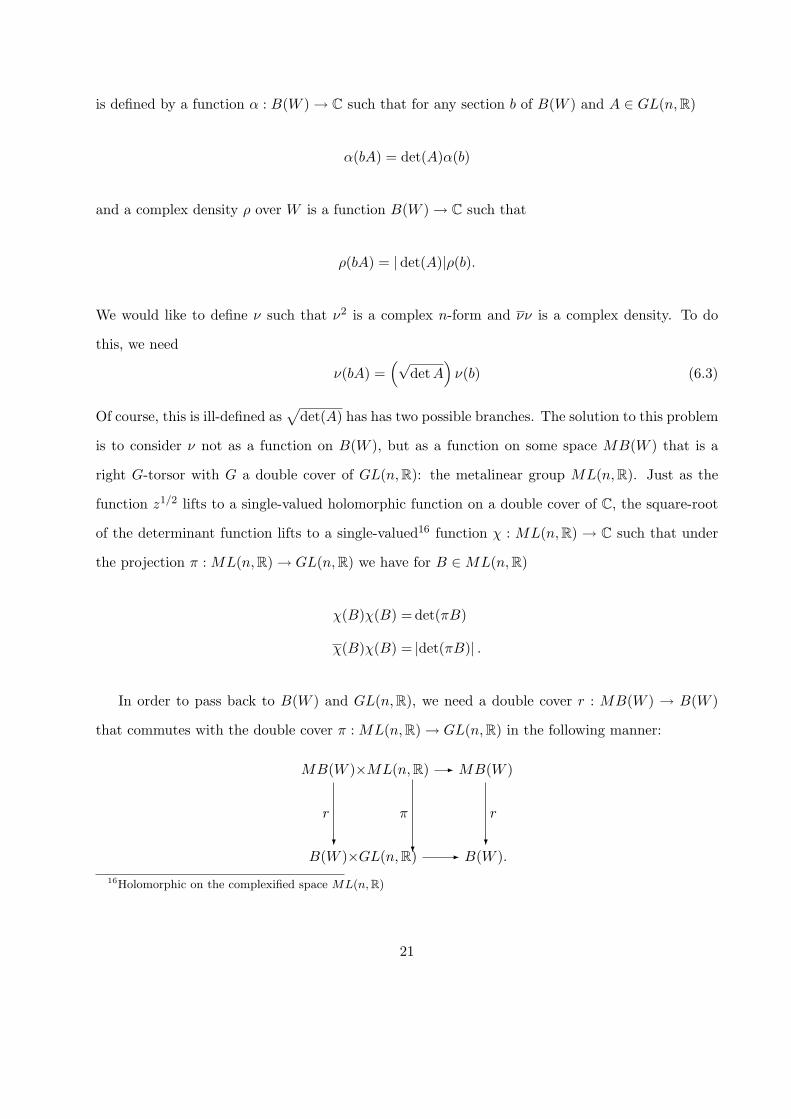
In order to pass back to B(W ) and GL(n,R), we need a double cover r : MB(W ) → B(W )

that commutes with the double cover π : ML(n,R) → GL(n,R) in the following manner:

MB(W )×ML(n,R) - MB(W )

B(W )×

r

?GL(n,R) -

π

?B(W ).

r

?

16Holomorphic on the complexified space ML(n,R)

21

With this construction, then for A ∈ML(n,R) and b ∈MB(W ), we use

ν(bB) = χ(B)ν(b) (6.4)

as our definition of half-forms. The space of all such forms forms a vector space Λ1/2W over C and

each element ν satisfies the correct requirements: ν2 is an n-complex volume form on W and νν is

a complex density.

The construction above passes immediately to a general manifold Q by “bundlizing.” We work

with the principal GL(n,R) bundle BQ, a principal ML(n,R) bundle MBQ, the commutative

diagram passes to a commutative bundle diagram and the construction above holds on each tangent

space TCQ. The only difficulties that arise are topological obstructions to the definition of MBQ

[5]. Assuming there are no such obstructions, however, we end up with the bundle of half-forms

Λ1/2T ∗CQ whose sections transform under metalinear transformations via (6.4).

6.3 The Metaplectic Group

The half-form construction on some Q = M/P solves the most difficult part of the construction of

the appropriate ν. However, a subtle issue still remains. The sections s are on a bundle over M ,

while the sections of Λ1/2T ∗CQ are over Q. However, in order to define a tensor product of B with

another bundle and talk about sections s⊗ν, we need both bundles to be over the same base space.

Furthermore, our construction was explicitly dependent on the polarization P (via the definition

of Q); we would like to have a better picture of half-forms that could possibly allow for comparison

between polarizations.

The basic idea is straightforward: we would like to somehow embed the ML(n,R) bundle

MBQ → Q into a “metaplectic” bundle of frames MB(M) over M . The half-forms, defined in

terms of their action on MBQ can then be extended to general frames over M by taking them to

be constant on metaplectic transformations which do not modify the embedding of MBQ.

The embedding should cover the natural embedding of the GL(n,R) bundle BQ→ Q into the

Sp(2n,R) bundle of frames SpB(M). So it is not hard to believe the so-called metaplectic group

Mp(2n,R) is taken to be the double cover of the symplectic group. Thus half-forms are intimately

22

related to the metaplectic group rather than the symplectic group; this leads to the interesting

insight that perhaps it is the metaplectic group (the double cover of the symplectic group) that

acts naturally in quantum mechanics rather than the symplectic group itself.

Thus, the half-form bundle Λ1/2T ∗CQ → Q can alternatively be viewed as a bundle over M

which we will refer to as δP (referring to the polarization P in the construction of Q).

6.4 The Real Quantization

Via the above construction, the bundle long sought is given as B = B ⊗ δP → M and, the inner-

product given by (6.1) and (6.2) is now appropriately defined on sections of B. One thing remains

before complete quantization: extending the covariant derivative to B. In fact, the covariant

derivative can be partially extended to complex n-forms µ over M , constant along P (ιXµ = 0 for

all X tangent to the leaves of P ) [1] via

∇Xµ =ιXdµ, ∀ X tangent to the leaves of P .

By using this and the fact that ν ∈ δP defines such a complex n-form ν2, then we can define a

covariant derivative on δP via the Leibnitz rule

∇Xν2 = 2(∇Xν)ν.

Similarly covariant differentiation of s = sν is also given by application of the Leibnitz rule.

Quantized sections are then square-integrable sections of B which are covariantly constant along

P .

6.5 Half forms in the Kahler Quantization

The requirement of half-forms in the real quantization lead to natural actions of the two-sheeted

covering groups ML(n,R) and Mp(2n,R) on our quantum sections. It is only natural to expect

that these groups, and the half-forms they act on, naturally arise in any polarization. Indeed, the

metaplectic group rears its head immediately in the case of Kahler polarizations. We will sketch

23

how this occurs, taking mostly from the discussion in [1].

Consider the Kahler quantization of a symplectic vector space V of dimension 2n. The quan-

tization procedure above introduced a space of square integrable sections HJ for each Kahler

polarization corresponding to the positive complex structure J . Now we can embed each HJ in the

space of all sections of B → M . Recall that we can quantize a classical observable f : M → R as

an operator f on the space of all sections, but only a restricted class of f lift to an f whose flow

preserves our HJ . We will put this observation in a different light: the flow of f : V → R is a

symplectomorphism on V and the lift of our flow (the flow of f thought of as a vector field on the

sections) furnishes a representation of such symplectomorphisms on the space of sections. However,

because the flow of f does not in general preserve HJ , this subspace does not generally furnish a

representation space for symplectomorphisms with respect to our quantization procedure.

However, we can attempt to rectify the situation by flowing a point in HJ along the vector field

in the space of sections defined by f , and continually projecting back onto HJ over every infinites-

imal time-step. It turns out this furnishes a projective representation of symplectomorphisms on

V . In fact, via the relationship between projective representations and representations of central

extensions (and covering groups), this representation is related to the metaplectic group (more

precisely, it is a representation of “metaplectomorphisms”).

Half-forms also pop into the picture. The assignment of a Hilbert space HJ to every positive

complex structure J ∈ L+V leads to a vector-bundle E → L+V whose fiber over J is HJ . If each

HJ is thought of as a subspace of the total space of sections of B → M , there is an orthogonal

projection operator between two fibers HJ and HJ ′ , to first order this creates a connection on our

bundle E. One can show this connection is “projectively flat,” i.e. the holonomy on our space is

multiplication by a complex phase factor. Hence, all fibers can be identified via our holonomy into

a single Hilbert space E. By quantizing linear symplectic transformations, we have a representation

of the symplectic group Sp(2n,R) on the entire space of sections E; however because our holonomy

is multiplication by a phase factor, this descends to a projective representation of the symplectic

group on V . Just as hinted above, this is a representation of the metaplectic group Mp(2n,R).

If we want a representation of the symplectic group, however, we must make the holonomy of

24

our line bundle E → F completely trivial. This can be done by twisting the bundle (via tensor

producting each fiber with some other space) to give the connection vanishing curvature. This

is where the half-forms arise: by changing each fiber to HJ ⊗ δPJ(i.e. tensor HJ with the half-

forms adapted to the polarization PJ) we obtain a bundle E′ with vanishing curvature (and trivial

holonomy). The identification space E is then a representation space for Sp(2n,R).

It should also be noted that, besides just giving an abstractly beautiful result, the half-form

modification HJ 7→ HJ ⊗ δPJgives the correct ground-state energy of the harmonic oscillator 1

2~,

a result that is not achieved with the representation of the harmonic oscillator Hamiltonian on the

space of sections HJ (see app. B).

7 Conclusion/Outlook

We have described enough of the geometric quantization construction to satisfactorily quantize a

very simple system, the n-dimensional harmonic oscillator, and only using a Kahler polarization.

Certainly the formalism developed here is applicable to other finite-dimensional systems and other

polarizations, especially if one employs the pairing mechanism alluded to earlier. However one clear

limitation of the program to date is that the final step in the program, the half-form construction or

metaplectic correction, cannot yet be carried out for systems with an infinite number of degrees of

freedom [3]. This is perhaps the most interesting class of systems as it includes field theories, some

of which (such as quantum electrodynamics) are very well understood, and some of which (such as

quantum general relativity) are not very well understood at all. Of course geometric quantization

is not necessarily the only or even always the best way to quantize a classical theory. Algebraic

procedures such as deformation quantization and Weyl quantization also serve to elucidate the

relationship between quantum and classical mechanics.

This may seem then like a lot of sophisticated mathematical machinery to develop only to

accomplish a relatively simple task, but in doing so we have set out on a path which we hope leads

to a deeper understanding of quantum mechanics and its geometric underpinnings. Canonical

quantization (which is contained in geometric quantization), often applied in physical applications,

is quite effective at producing a meaningful and practically applicable quantum theory. However, it

25

is based on particular position and momentum coordinates (i.e. a single polarization) without giving

insight into how quantizations based on other polarizations are related; it is not clear from that

perspective how quantizing could be a “symplectically invariant” procedure. In contrast, the tools

developed by geometric quantization such as the pairing mechanism give a very clear picture of how

these different quantization procedures based on different polarizations are related. Furthermore,

both the pairing mechanism, which involves projective representations, and the natural emergence

of the metaplectic group appear to be geometric manifestations of a deep connection between

quantum mechanics and central extensions of the symplectic group. This connection remains to be

fully explored.

26

A Holonomies of a Complex Line Bundle

We first begin by choosing a line bundle π : B → M with connection ∇ and choose a local

trivialization (U, τ) for some neighborhood U ⊂ M and τ : M × C → π−1(U). The trivialization

yields a unit section s = τ(·, 1) from which we can define the potential one-form Θ ∈ Ω1(U) via

∇s = −iΘs.

Now any section s over U can be written as s = ψs for some complex-valued function ψ ∈ ω0(U);

for any such general section then,

∇Xs =(X(ψ)− iιXΘ) s

=(dψ(X)− iιXΘ) s

=ιX (d− iΘ)ψs

To construct the holonomy operator, we first consider a closed curve γ : [0, 1] → U parameterized

by t ∈ [0, 1], s = ψs a section over the image of γ, and γ the tangent vector field defined over the

image of γ. Then s is parallel to γ if

0 =∇γs

=(dψ

dt− iιγΘψ

)s.

This is an ODE in ψ with (unique) solution

ψ(t) = exp(it

∫γΘ

)ψ(0);

27

thus, the holonomy operator around a closed curve γ is given by multiplication by the complex

number

ξ = exp(i

∫γΘ

).

B Operators

Here we construct all self-adjoint operators that preserve a Kahler polarization.

Using the metric to raise or lower indices, e.g. pa = gabpb, introduce the complex coordinates

za =pa + iqa za =pa − iqa pa = 12(z + z) qa =− 1

2i(z − z)

then

dza = dpa + idqa dza = dpa − idqa ∂

∂za=

12

(∂

∂pa− i

∂

∂qa

)∂

∂za=

12

(∂

∂pa+ i

∂

∂qa

)

and the Hamiltonian vector field of a function f (eq. 1.7) is

Xf = −2i(∂f

∂za

∂

∂za− ∂f

∂za

∂

∂za

). (B.1)

We have a Kahler polarization P whose leaves are surfaces of constant za so that vectors

tangent to leaves lie in the span of ∂∂za . For the flow of a Hamiltonian vector field Xf to preserve

the polarization it must Lie drag vectors tangent to P into vectors tangent to P (eq. 5.2)

LXf

(∂

∂za

)=

[Xf ,

∂

∂za

]=

∂

∂za(Xf ) = 2i

(∂2f

∂za∂zb

)∂

∂zb− 2i

(∂2f

∂za∂zb

)∂

∂zb⇒ ∂2f

∂za∂zb= 0

(B.2)

which, together with the requirement that f is an observable and hence real, restricts f to be of

the form (eq. 5.3)

f = 12iwaz

a − 12iwaza + 1

2Uabz

azb + c (B.3)

where w and c are complex constants, and Uab = Uba.

28

The explicit forms of wavefunctions and operators depend on the choice of gauge, a particular

symplectic potential θ (app. C). In the gauge adapted to P ,

θ = padqa = − 1

2izadz

a, (B.4)

the wave functions ψ = φν are the product of φ(z) a holomorphic function on M (a section of

the prequantum bundle B) and a half-form ν (a section of the half-form bundle). Note that if we

choose a standard volume form µ of P, any other volume form is a complex function of z times

µ. Similarly any half-form is a complex function of z times√µ, so in our wavefunctions we may

absorb the extra function into φ and always choose ν =√µ without loss of generality. Explicitly,

ψ = φ′(z)ν ′ = φ′(z)g(z)√µ = φ(z)

õ (B.5)

Denote by f an operator acting on ψ and by f an operator acting on φ(z) only. A function f

determines an operator f via

f = −i~(LXf

− i

~ιXf

θ

)+ f (B.6)

and

fψ = (fφ)√µ− i~φLXf

õ (B.7)

where f is defined in eq. 3.1. First we compute the operator f corresponding to an f whose Xf

preserves P (eq. B.3),

f = −i~Xf + f − ιXfθ

= −i~(

2i∂f

∂za

∂

∂za

)+ f − (− 1

2iza)

(2i∂f

∂za

)= 2~

∂f

∂za

∂

∂za+

(f − za

∂f

∂za

)= −i~wa ∂

∂za+ ~Uabza

∂

∂zb+ 1

2iwaz

a + c.

The choice w = c = 0 and Uab = δab yields the Hamiltonian h of the n-dimensional harmonic

29

oscillator, so h is as given in eq. 5.4,

h = ~za ∂

∂za. (B.8)

Next we compute the extra Lie derivative term in f . We take as our standard volume form

µ = (4π~)n/2µ0 where µ0 = dnz = dz1 ∧ · · · ∧ dzn, and our standard half-form ν =√µ, then

compute

LXfµ0 = d

(ιXf

dnz)

= 2i d(∂f

∂zaι ∂

∂zadnz

)= wad

(ι ∂

∂zadnz

)+ i d

(U a

b zbι ∂∂za

dnz)

= i div(U a

b zb)µ0 = i

(∂

∂zaU a

b zb

)µ0 = i

(U a

b δba

)µ0 = i (trU)µ0

LXfµ = i (trU)µ

= LXfν2 = 2νLXf

ν

LXfν = 1

2i (trU) ν

−i~φLXf

õ = 1

2~ (trU)

õ

so that the operator f is

fψ =((f + 1

2~ trU

)φ)√

µ (B.9)

or, with the understanding that derivatives act only on φ(z),

f = −i~wa ∂

∂za+ ~Uabza

∂

∂zb+ 1

2iwaz

a + c+ 12~ trU. (B.10)

The choice w = c = 0 and Uab = δab (the Hamiltonian h of the n-dimensional harmonic oscillator),

using tr δ = n, now yields the operator h

h = ~(za ∂

∂za+ 1

2n

)(B.11)

which has the correct eigenvalue spectrum. For example the one-dimensional harmonic oscillator

(n = 1) has eigenvalues ~(N + 12) corresponding to eigenfunctions φ(z) that are homogeneous

polynomials in z of degree N .

30

C Coherent States

Define

∂ = dza ∧ ∂

∂za∂ = dza ∧ ∂

∂zad = dpa ∧

∂

∂pa+ dqa ∧ ∂

∂qa= ∂ + ∂

and now in terms of the Kahler scalar K we have

K = 12gabz

azb ω = i∂∂K (C.1)

θ = − 12izadz

a θ0 = 12(padq

a − qadpa) (C.2)

= 12(padq

a − qadpa)− 12i(padp

a + qadqa) = θ + 1

2idK. (C.3)

If we have a Kahler polarization P the wavefunctions take a simple form in the θ gauge adapted

to P , that is they are simply holomorphic functions φ(z). However, as discussed earlier in section

(3.3) the inner product takes a simple form in a gauge such as θ0 where the symplectic potential is

real. The wavefunctions in the θ0 gauge are

φ′(z, z) = φ(z) exp(−K

2~

)= φ(z) exp

(−gabz

azb

4~

)(C.4)

and the inner product of two wavefunctions φ1 and φ2 is

〈φ1, φ2〉 =∫

Pφ1φ2 exp

(−gabz

azb

2~

)ε. (C.5)

Note that if g is positive-definite the exponential factor ensures that the integral is finite as long as

φ1 and φ2 are sufficiently well-behaved (i.e. are bounded and do not grow exponentially or faster

with large z).

Such holomorphic wavefunctions φ(z) may be viewed as the Bargmann transform of wavefunc-

tions on real phase space[6].

31

References

[1] N. M. J. Woodhouse, Geometric Quantization (Oxford University Press, UK, 1991).

[2] D. J. Simms and N. M. J. Woodhouse, Lectures on Geometric Quantization (Springer-Verlag,

Berlin, 1976).

[3] T. Thiemann, Modern Canonical Quantum General Relativity (Cambridge University Press,

UK, 2007).

[4] B. Kostant, Bull. Amer. Math. Soc. 73, 692 (1985).

[5] V. Guillemin and S. Sternberg, Geometric Asymptotics (American Mathematical Society, Prov-

idence, RI, 1977).

[6] G. B. Folland, Harmonic Analysis in Phase Space (Princeton University Press, Princeton, New

Jersey, 1989).

32