Renormalization of Quantum Electrodynamics1

D. E. Soper2

University of OregonPhysics 666, Quantum Field Theory

May 2001

1 The action

Most of the calculations that one does in quantum field theory beyond theleading order lead to ultraviolet divergences. In these notes, we see how todeal with that.

The first step is to look at the action. (We consider quantum electro-dynamics since it is perhaps the most important relativistic quantum fieldtheory, but the ideas are quite general.) The action is

S =∫ddx

[ψ0(x)i/∂ −Qe0/A(x)−m0ψ0(x)− 1

4F µν

0 (x)F0,µν(x)]. (1)

Here I have called the fields ψ0 and Aµ0 , with F µν0 (x) ≡ ∂µAν0 − ∂νAµ0 . These

are the “bare fields.” Also, the coupling is e0, the “bare coupling” and themass is m0, the “bare mass.” This is like a corperate reorganization, whereevery job gets a new title.

I have also anticipated that we may want to operate in

d = 4− 2ε (2)

dimensions of space-time. Thus we have∫ddx.

All of this business with dimensional regulation is not so important forthe moment. What is important is that we recogize that the bare quantitiesmay not be upon which to base our perturbation theory. Instead, we candefine renormalized quantities by

ψ0 = µ−ε√Zψ ψ

Aµ0 = µ−ε√ZAA

µ

m0 = Zmm

g0 = µεZg g. (3)

1Copyright, 2001, D. E. Soper2soper@bovine.uoregon.edu

1

In these relations, I have introduced a quantity µ with the dimensions of mass(or momentum or inverse distance). The idea is this: S is dimensionless,while ddx has dimensions m−d = m−4 × m2ε. Thus the bare fields and thebare coupling have dimensions that depend on ε. On the other hand, I wantthe ψ,Aµ,m and g to have fixed dimensions, independent of ε and I want thevarious factors Z to be dimensionless. Thus I put the proper dimensionfulfactor equal to a power of µ in front of each Z.

Then

S = µ−2ε∫ddx

[ψ(x)Zψi/∂ − Zψ

√ZAZeQe/A(x)− ZψZmmψ(x)

−14ZAF

µν(x)Fµν(x)]. (4)

This doesn’t seem very helpful, but we can make it even worse:

S = µ−2ε∫ddx

[ψ(x)i/∂ −mψ(x)− 1

4F µν(x)Fµν(x)

−ψ(x)Qe/A(x)ψ(x)

+(Zψ − 1) ψ(x)i/∂ψ(x)

−(Zψ√ZAZe − 1) ψ(x)Qe/A(x)ψ(x)

−(ZψZm − 1) ψ(x)mψ(x)

−(ZA − 1)14F µν(x)Fµν(x)

]. (5)

Although this looks like a mess, it does something good. We can treat the firsttwo terms as the unperturbed action that provides the basis for perturbationtheory. All the other terms are treated as perturbations. This includes theterms proportional to powers of various Zs minus 1.

These terms are treated as perturbations and generate “counterterms”in the Feynman diagram expansion of the theory. Let’s write the rules inmomentum space. I should mention that when we go from position spaceto momentum space in the renormalized theory we will defne the Fouriertransform by

µ−2ε∫d4−2εx eik·x (6)

so that the Fourier transformed renormalized fields have fixed dimensions.Then each integral over a loop momentum will come out to have the form

µ2ε∫ d4−2εk

(2π)4−2ε(7)

2

which is just right to keep the dimensionality fixed if we add loops.Here are the Feynman rules. We have the usual interaction

−ieQγµ (8)

but now we have counterterms

• Electron field strength renormalization counterterm

i(Zψ − 1)/k (9)

• Electron mass counterterm

−i(ZψZm − 1)m (10)

• Photon field strength renormalization counterterm

i(ZA − 1)(−gµνq2 + qµqν) (11)

• Vertex counterterm

−i(Zψ√ZAZe − 1) eQγµ (12)

2 Integrals

When we compute Feynman diagrams in d dimensions, we will need theintegral

I =∫ ddk

(2π)d1

[k2 − Λ2 + iε]A. (13)

Let’s see how to do this.First, we rotate the k0 integration to the imaginary axis, so k0 = iκ.

Then

I =∫ dκ dd−1~k

(2π)di

[−κ2 − ~k2 − Λ2]A=∫ dκ dd−1~k

(2π)di(−1)A

[κ2 + ~k2 + Λ2]A. (14)

We write this as an integration over a vector space with a euclidian metric(“E”):

I = i(−1)A∫E

ddk

(2π)d1

[k2 + Λ2]A. (15)

3

Now use the integral representation of the gamma function to write

I =i(−1)A

Γ(A)

∫E

ddk

(2π)d

∫ ∞

0

dλ

λλA exp−λ[k2 + Λ2]

=i(−1)A

Γ(A)

∫ ∞

0

dλ

λλAe−λΛ2

∫E

ddk

(2π)dexp−λk2 (16)

Here is where we come to the meaning of d dimensions. If d is an integer, wehave

k2 =d∑j=1

k2j (17)

so ∫E

ddk

(2π)dexp−λk2 =

(∫ ∞

−∞

dk

2πexp−λk2

)d(18)

We make this the definition if d is not an integer. Of course, we know theintegral: ∫ ∞

−∞dx exp−x2 =

√π, (19)

so ∫ ∞

−∞

dk

2πexp−λk2 =

1√4πλ

. (20)

Thus

I =i(−1)A

Γ(A)

∫ ∞

0

dλ

λλAe−λΛ2

[4πλ]−d/2

=i(−1)A

Γ(A)[4π]−d/2

∫ ∞

0

dλ

λλA−d/2e−λΛ2

=i(−1)A

Γ(A)[4π]−d/2 Λd−2A Γ(A− d/2) (21)

That is ∫ ddk

(2π)d1

[k2 − Λ2 + iε]A=i(−1)A

Γ(A)[4π]−d/2

Γ(A− d/2)

[Λ2]A−d/2. (22)

Note that the power of Λ2 follows by power counting. Recall that Γ(z) hasa pole at z = 0 (and also at positive integer values of z). Thus our integral

4

has a pole at just the point where the power of Λ2 is zero. Near z = 0 onehas

Γ(z) =1

z− γE +O(ε). (23)

where γE is the Euler constant, 0.577 · · ·.Sometimes, one needs the integral∫ ddk

(2π)dkµ

[k2 − Λ2 + iε]A. (24)

This integral is zero because it is odd under kµ → −kµ. Also, one canencounter ∫ ddk

(2π)dkµkν

[k2 − Λ2 + iε]A. (25)

This is easy to evaluate by replacing

kµkν → 1

dgµν k2 (26)

and writing k2 as (k2 − Λ2) + Λ2.

3 The electron propagator

The 1PI graph has a name: −iΣ. We have

−iΣ(p) = −e2µ2ε∫ d4−2εq

(2π)4−2ε

γµ(/p− /q +m)γµ[(p− q)2 −m2 + iε][q2 + iε]

(27)

Using a Feynman parameter α this becomes

−iΣ(p) = −e2∫ 1

0dα µ2ε

∫ d4−2εq

(2π)4−2ε

γµ(/p− /q +m)γµ[q2 − Λ2 + iε]2

(28)

whereqµ = qµ − αpµ (29)

andΛ2 = αm2 − α(1− α)p2. (30)

The numerator becomes

γµ((1− α)/p− /q +m)γµ (31)

5

We can throw away the q term since it integrates to zero. For the otherterms, we use our γµΓγµ rules, giving

−2(1− ε)(1− α)/p+ (4− 2ε)m (32)

Thus

−iΣ(p) = −e2∫ 1

0dα µ2ε

∫ d4−2εq

(2π)4−2ε

−2(1− ε)(1− α)/p+ (4− 2ε)m

[q2 − Λ2 + iε]2(33)

Now we can perform the q integration, giving

−iΣ(p) =−ie2

(4π)2Γ(ε)

∫ 1

0dα

(4πµ2

Λ2

)ε[−2(1− ε)(1− α)/p+ (4− 2ε)m], (34)

or

Σ(p) =αem

4πΓ(ε)

∫ 1

0dα

(4πµ2

Λ2

)ε[−2(1− ε)(1− α)/p+ (4− 2ε)m] . (35)

To use this result, we add in the counter terms and expand around ε = 0:

Σ(p) =αem

4π

1

ε(1− εγE + · · ·)

∫ 1

0dα

[1 + ε ln

(4πµ2

Λ2

)+ · · ·

]× [−2(1− ε)(1− α)/p+ (4− 2ε)m] + C.T.

=αem

4π

1

ε

∫ 1

0dα [−2(1− α)/p+ 4m]

+αem

4π

∫ 1

0dα ln

(4πµ2

Λ2e−γE

)[−2(1− α)/p+ 4m]

+αem

4π

∫ 1

0dα [2(1− α)/p− 2m] + · · ·+ C.T.. (36)

In the first and last terms, we can perform the α itegration immediately,while we leave the integration undone in the second term. We simplify thesecond term with the substitution

4πµ2 e−γE ≡ µ2. (37)

Then

Σ(p) =αem

4π

1

ε[−/p+ 4m]

+αem

4π

∫ 1

0dα ln

(αm2 − α(1− α)p2

µ2

)[2(1− α)/p− 4m]

+αem

4π[/p− 2m] + · · ·

−(Zψ − 1)/p+ (ZψZm − 1)m. (38)

6

Now we get to choose what (Zψ − 1) and (ZψZm − 1) are. These quantitieswill have expansions in powers of αem. At our current order of perturmbationtheory, we are only concerned with the α1

em contributions.We can choose the “modified minimal subtraction” prescription, usually

denoted MS. In this prescription, we choose the counter terms to cancel thepoles and no more:

(Zψ − 1) = −αem

4π

1

ε+O(α2

em)

(ZψZm − 1) = −αem

π

1

ε+O(α2

em). (39)

With the MS prescription we have

Σ(p) =αem

4π

∫ 1

0dα ln

(αm2 − α(1− α)p2

µ2

)[2(1− α)/p− 4m]

+αem

4π[/p− 2m] + · · · . (40)

This is an analytic function of p2 for spacelike pµ, that is p2 < 0. It hasa branch point at p2 = m2, corresponding to an electron splitting into anelectron and a photon. We may consider that the function has a branch cutfrom p2 = m2 to p2 = ∞. The physical side of the branch cut is Im(p2) > 0.

This may seem very strange. We seem to be hiding something infinitewith the (Z−1) trick while all the time we are expanding in a small quantityαem. How can we expand in powers of αem × ∞? A way to think of thisis that our integralions really end at q2 ∼ M2, where M2 is a momentumscale beyond our experimental reach. For instance M = 10 TeV. Beyondthe scale M2 there is some new physics that we don’t know about. We maysuppose that below M2 we have Standard Model physics, for which we havejust calculated the most important diagram. The “bare” quantities refer tothe effective action that applies at scale M2 and below.

Now if we perform the integrations with a cutoff around M2, we will getα0 ln(p2/M2) factors. (There is a log because the integration is logarithmi-cally divergent.) Then we use the (Z − 1) trick to change to “renormalized”quantities with

(Z − 1) ∼ (const)αem

πln(M2/µ2) +O(α2

em) (41)

This cancels the ln(M2) and replacees it by ln(µ2), where µ can be of theorder of the electron mass. Thus the renormalized expansion has powers of

7

αem multiplied by quantities of order 1. This compares to the unrenormal-ized perturbation theory, which has powers of α0 ln(M2/“m2

e”) and hencedoes not converge so well. As a technical trick, we don’t just cut off theintegrations, but rather regulate them with dimensional regulation. Thus weshould understand µ2ε/ε as a stand in for ln(µ2/M2).

Exercise: Calculate the photon self energy Πµν at one loop order to obtaina formula analogous to Eq. (35), that is Πµν in 4 − 2ε dimensions beforesubtracting the counter term.

4 Structure of the propagator

We will want to investigate on-shell renormalization. Before starting this,let’s look at the complete propagator iD(p). Let −iΣ(p) be the one parti-cle irreducible two point function for the electron, summed to all orders ofperturbation theory. Then we have

D(p) =1

/p−m

1 + Σ(p)1

/p−m+

(Σ(p)

1

/p−m

)2

+ · · ·

. (42)

This sums to

D(p) =1

/p−m

[1− Σ(p)

1

/p−m

]−1

. (43)

We can simplify this, being careful of the matrix ordering: If we let E = /p−m,we have

D = E−1(1− ΣE−1)−1 (44)

soD(1− ΣE−1) = E−1 (45)

soD(E − Σ) = 1 (46)

orD = (E − Σ)−1. (47)

That isD(p) = [/p−m− Σ(p)]−1 (48)

8

Thus if we knew Σ(p) exactly, we would have the inverse of the propaga-tor.

We can carry this a little further by writing

Σ(p) = A(p2)[/p−m] +B(p2)m. (49)

Then

D =1

1− A(p2)

/p+ (1 + C(p2))m

p2 − (1 + C(p2))2m2(50)

where

C(p2) =B(p2)

1− A(p2). (51)

We see that (if C is close to 0) D has a pole at some value of p2 which maynot be m2. The residue of this pole may not be 1. Note that we have to sumthe series (42) in order to see that the pole moves. We do not, however, haveto sum all of the contributions to Σ to see this.

5 On-shell renormalization

We can adjust the Z − 1 factors to make m the physical electron mass, thatis, the location of the pole. Evidently, what we need is

B(m2) = 0, (52)

so that C(m2) = 0. We can also adjust the Z− 1 factors to make the residueof the pole at p2 = m2 equal to /p+m:

D(p) ∼ /p+m

p2 −m2as p2 → m2. (53)

With a little algebra, we find that the required condition is

A(m2) = 2m2B′(m2). (54)

We can call Eqs. (52) and (54) the on-shell renormalization conditions.Let’s work this out. But first, we give the photon a small mass mγ in

order to control certain infrared divergences that we don’t want to worryabout yet. If we give a mass to the photon, our previous analysis worksexcept that the denominator function becomes

Λ2 = αm2 + (1− α)m2γ − α(1− α)p2. (55)

9

Then let us imagine that we write the counter terms as a[/p−m] + bm where

a =apole

ε+ a′

b =bpole

ε+ b′ (56)

where the first parts are the counterterms in the MS prescription and a′ and b′

are additional pieces that we now add to satisfy the on-shell renormalizationconditions. Once we have subtracted the pole terms, we can take ε → 0 (aslong as mγ 6= 0). (Peskin and Schroeder do this with ε 6= 0 but then it is alittle more messy.) We find

Σ(p) =αem

4π

∫ 1

0dα ln

(αm2 + (1− α)m2

γ − α(1− α)p2

µ2

)× [2(1− α)(/p−m)− 2(1 + α)m]

+αem

4π[(/p−m)−m] + a′(/p−m) + b′m (57)

The functions A and B have the form

A(p2) = A1(p2) + a′

B(p2) = B1(p2) + b′, (58)

where A1(p2) and B1(p

2) are the one-loop functions that we read off fromEq. (57) and a′ aned b′ are the corresponding counterterms, which are inde-pendent of p2. The solution of the on-shell renormalization conditions (52)and (54) is

a′ = −A1(m2) + 2m2B′

1(m2)

b′ = −B1(m2). (59)

We have

A1(p2) =

αem

4π

∫ 1

0dα

ln

(αm2 + (1− α)m2

γ − α(1− α)p2

µ2

)2(1− α) + 1

B1(p2) =

αem

4π

∫ 1

0dα

×− ln

(αm2 + (1− α)m2

γ − α(1− α)p2

µ2

)2(1 + α)− 1

. (60)

10

Then

B′1(p

2) =αem

4π

∫ 1

0dα

2α(1− α2)

αm2 + (1− α)m2γ − α(1− α)p2

. (61)

Thus

a′ =αem

4π

∫ 1

0dα− ln

(α2m2 + (1− α)m2

γ

µ2

)2(1− α)− 1

− 4α(1− α2)

α2 + (1− α)m2γ/m

2

b′ =αem

4π

∫ 1

0dαln

(α2m2 + (1− α)m2

γ

µ2

)2(1 + α) + 1

. (62)

Putting this together, we have

Σ(p) =αem

4π

∫ 1

0dαln

(αm2 + (1− α)m2

γ − α(1− α)p2

α2m2 + (1− α)m2γ

)× [2(1− α)(/p−m)− 2(1 + α)m]

− 4α(1− α2)(/p−m)

α2 + (1− α)m2γ/m

2

. (63)

The details of this result are not so important. The most important featureare that the dependence on µ has disappeared. It didn’t really matter how weregulated the integral. Also, the on-shell renormalization is pretty much likethe MS renormalization with the scale µ of the order of the electron mass.Finally, note that if we set mγ to zero we will have a logarithmic divergencefrom the α→ 0 region in the integral.

The logarithmic divergence when mγ = 0 arises because, if mγ = 0, theelectron propagator doesn’t really have a pole. We can illustrate this asfollows. If we start from Eq. (57) with mγ = 0 and use the on-shell value forb′ so that the location of the singularity in the propagator is at p2 = m2 ( sothat m = me) but use the MS value for a′, namely a′ = 0, we get

Σ(p) =αem

4π

∫ 1

0dα

×

ln

(αm2

e − α(1− α)p2

µ2

)2(1− α) + 1

(/p−me)

−αem

4π

∫ 1

0dα ln

(αm2

e − α(1− α)p2

α2m2e

)2(1 + α)me. (64)

11

This is a finite result for p2 < m2e. The coefficient B(p2) of m vanishes

at p2 = m2e, so that p2 = m2

e is where the singularity of the propagator islocated. However

B(p2) = −αem

4π

∫ 1

0dα ln

(1− 1− α

α

p2 −m2e

m2e

)2(1 + α). (65)

As p2 → m2e, this function does not behave like p2 −m2

e, but rather like

(p2 −m2e) ln(p2 −m2

e) (66)

This term will dominate the denominator in Eq. (50), so that instead ofhaving a pole, D(p2) behaves like

const.

(p2 −m2e) ln(p2 −m2

e). (67)

The consequence is that, with the on-shell renormalization prescription,the renormalized Green functions depend on an artificial cutoff parameter,mγ. Only when we calculate a physical observable will the mγ dependencedisappear in the limit mγ → 0.

Compare this with the MS prescription, in which the renormalized elec-tron propagator is perfectly finite in the physical case mγ = 0 as long as westay away from p2 = m2

e.If we calculate electron-electron scattering at one loop order, then the on-

shell renormalization prescription is the most convenient. But, however wedo it, we will have to deal with an infrared divergence that can be regulatedby taking mγ 6= 0. The problem is that on-shell electron-electron scatteringis not physically observable. Real electrons are always accompanied by softphotons – photons that have arbitrarily small momenta. We have to buildinto the calculation the fact that some of the photons are too soft to bedetected before we can get an answer for electron-electron scattering that isfinite when mγ → 0.

Another way to regulate the soft photon divergence is by staying in 4−2εdimensions. In this style of calculation, with on-shell renormalization, therenormalized electron propagator has some 1/ε terms. The renormalizationsubtraction gets rid of the 1/ε terms that come from ultraviolet momentain the loop. But then renormalization subtraction adds 1/ε terms associ-ated with infrared momenta and arise from the unphysical renormalizationcondition.

12

6 The photon propagator

The 1PI graph is generally called −iΠµν (or +iΠµν in the notation of Peskinand Schroeder). At one loop we have

−iΠµν(q) = −e2µ2ε∫ d4−2εk

(2π)4−2ε

Tr [γµ(/k − /q +m)γν(/k +m)]

[(k − q)2 −m2 + iε][k2 −m2 + iε]+ C.T.

(68)We already know how to do this kind of calculation, so I will leave out

the intermediate steps, except to point out that in one of the terms we get afactor

−1 + ε

−2 + ε[−Γ(−1 + ε) + Γ(ε)] =

1

−2 + ε[−Γ(ε) + (−1 + ε)Γ(ε)] = Γ(ε). (69)

The result is

Πµν(q) = 2αem

πΓ(ε) (gµνq2 − qµqν)

∫ 1

0dα α(1− α)

(m2 − α(1− α)q2

4πµ2

)−ε

+αem

π(gµνq2 − qµqν)

(− 1

3ε+ δc

). (70)

The second line is the counter term, which, according to the Feynman rules,must be proportional to (gµνq2 − qµqν). If we choose MS renormalization,then the counter term is simply the pole term and the extra constant that Ihave called δc is zero. That is

(ZA − 1) = −αem

3π

1

ε+O(α2

em). (71)

Since the pole term gets rid of the divergence, we can take the limit ε→ 0to get (with any renormalization prescription)

Πµν(q) = −2αem

π(gµνq2 − qµqν)

∫ 1

0dα α(1− α) ln

(m2 − α(1− α)q2

µ2

)

+αem

π(gµνq2 − qµqν)δc. (72)

If we would like to use on-shell renormalization, we need a little analysis ofthe photon propagator. (We stick to Feynman gauge, for simplicity.) Define

C(q)µν = gµν −qµqνq2

. (73)

13

Note the properties

C(q)µνqν = 0, C(q)µλC(q)λν = C(q)µν . (74)

We can define Π(q2) by

Πµν(q) = −q2C(q)µνΠ(q2). (75)

Then the complete photon propagator is

Dµν =−gµν

q2+−gµν

q2(−q2C(q)αβΠ(q2))

−gαν

q2+ · · · (76)

This is

Dµν = − 1

q2

qµqν

q2− C(q)µν

q2

[1 + Π(q2) + Π(q2)2 + · · ·

]. (77)

There is an orphan qµqν term, but then a geometric series. Summing theseries, we have

Dµν = − 1

q2

qµqν

q2− C(q)µν

q2[1− Π(q2)]. (78)

There is some real physics content here. Because Πµν has the structure givenin Eq. (75), the pole in the photon propagator remains at q2 = 0.

Now to implement on-shell renormalization, we adjust the counter-termsso that

Π(0) = 0. (79)

Then

Dµν ∼ − 1

q2

qµqν

q2− C(q)µν

q2= −g

µν

q2. (80)

as q2 → 0.With on-shell renormalization, we have

Πµν(q) = −2αem

π(gµνq2 − qµqν)

∫ 1

0dα α(1− α) ln

(m2 − α(1− α)q2

m2

)(81)

Recall that the counter term that adjusts Πµν is

(ZA − 1)(gµνq2 − qµqν). (82)

14

Our next exercise will be an investigation of the renormalization of the 1PIelectron-photon vertex. We will find then that Ze = 1/

√ZA. Thus when

we decide on the renormalization prescription for the photon propagator,we are really deciding how to define the unit of electric charge squared,e2/(4π) = αem. With the MS definition, we get a definition that dependson the scale µ: αem(µ2). With the on-shell definition, we get the standardcoupling that is usually called simply αem and is approximately 1/137. Wehave seen that to one-loop accuracy, and if electron are the only chargedfermions, αem = αem(m2

e).

7 Renormalization of the vertex function

We now examine the eeγ vertex function, Γµ. our aim is to see what counterterm we have to include in Γµ to make it finite. The calculation starts as inthe calculation of the electron anomalous magnetic moment, except that wedo not necessarily take the incoming and outgoing electrons to be on-shell.We have

Γµ = −ie2µ2ε∫ d4−2εl

(2π)4−2ε

γα(/k′ − /l +m)γµ(/k − /l +m)γα[(k′ − l)2 −m2 + iε][(k − l)2 −m2 + iε][l2 + iε]

+C.T.. (83)

For our limited purposes, we do not need to introduce Feynman parameters,but let’s do so so that we can follow along with the complete calculation ofΓµ for awhile. With Feynman parameters, we have

Γµ = −2ie2∫ 1

0dα∫ 1−α

0dβ µ2ε

∫ d4−2εl

(2π)4−2ε

×γα(/k′ − /l +m)γµ(/k − /l +m)γα

[D2 + iε]3

+C.T., (84)

where

D = α[(k′ − l)2 −m2] + β[(k − l)2 −m2] + (1− α− β)l2

= l2 − 2αk′ · l − 2βk · l + α(k′2 −m2) + β(k2 −m2)

= (l − αk′ − βk)2 + α(1− α)k′2 + β(1− β)k2 + 2αβk · k′ − (α+ β)m2

= l2 − Λ2. (85)

15

Here the shifted loop momentum is

lµ = lµ − αk′µ − βkµ. (86)

If we use γ = 1− α− β and qµ = k′µ − kµ, we can write Λ2 in a nice form:

Λ2 = −αγk′2 − βγk2 − αβq2 + (α+ β)m2 (87)

Thus

Γµ = −2ie2∫ 1

0dα∫ 1−α

0dβ µ2ε

∫ d4−2εl

(2π)4−2ε

×γα((1− α)/k′ − β/k − /l +m)γµ(−α/k′ + (1− β)/k − /l +m)γα

[l2 − Λ2 + iε]3

+C.T., (88)

So far, we have a complete calculation. Now we concentrate on piecesthat can give a 1/ε, which are those arising from having two factors of lν inthe numerator. We have

γα/lγµ/lγα = −2(1− ε)/lγµ/l

→ − (1− ε)

2(1− ε/2)l2 γβγ

µγβ

= − (1− ε)2

(1− ε/2)l2 γµ

= − (1− ε)2

(1− ε/2)(l2 − Λ2) γµ − (1− ε)2

(1− ε/2)Λ2 γµ. (89)

In the step indicated by an arrow, we have used the fact that lαlβ andl2gαβ/(4− 2ε) have the same integral.

The second term of this result will not give a divergence as ε → 0. Andin the first term, we can set ε → 0 in the coefficient if all we want is thecoefficient of 1/ε. Then

Γµ = −2ie2∫ 1

0dα∫ 1−α

0dβ µ2ε

∫ d4−2εl

(2π)4−2ε

γµ

[l2 − Λ2 + iε]2

+C.T.+ finite. (90)

16

We perform the lν integration to get

Γµ = −2ie2γµ∫ 1

0dα∫ 1−α

0dβ i[4π]−(2−ε)Γ(ε)[Λ2/µ2]−ε

+C.T.+ finite

=αem

2πγµ∫ 1

0dα∫ 1−α

0dβ Γ(ε)

[Λ2

4πµ2

]−ε+C.T.+ finite

=αem

4πγµ

1

ε+C.T.+ finite. (91)

It should be evident from this derivation how we could keep all of the finiteterms. But if we want just the MS counter term, it is C.T. = (Zψ

√ZAZe−1)

with

(Zψ√ZAZe − 1) = −αem

4π

1

ε+O(α2

em). (92)

Recall that we found (with the MS prescription)

(Zψ − 1) = −αem

4π

1

ε+O(α2

em)

(ZψZm − 1) = −αem

π

1

ε+O(α2

em). (93)

and

(ZA − 1) = −αem

3π

1

ε+O(α2

em). (94)

Thus

Zψ = 1− 1

4

αem

π

1

ε+O(α2

em)

ZA = 1− 1

3

αem

π

1

ε+O(α2

em)

Zm = 1− 3

4

αem

π

1

ε+O(α2

em)

Ze = 1 +1

6

αem

π

1

ε+O(α2

em). (95)

If we want to use on-shell renormalization, we have to consider

U(k′, s′)ΓµU(k, s) (96)

17

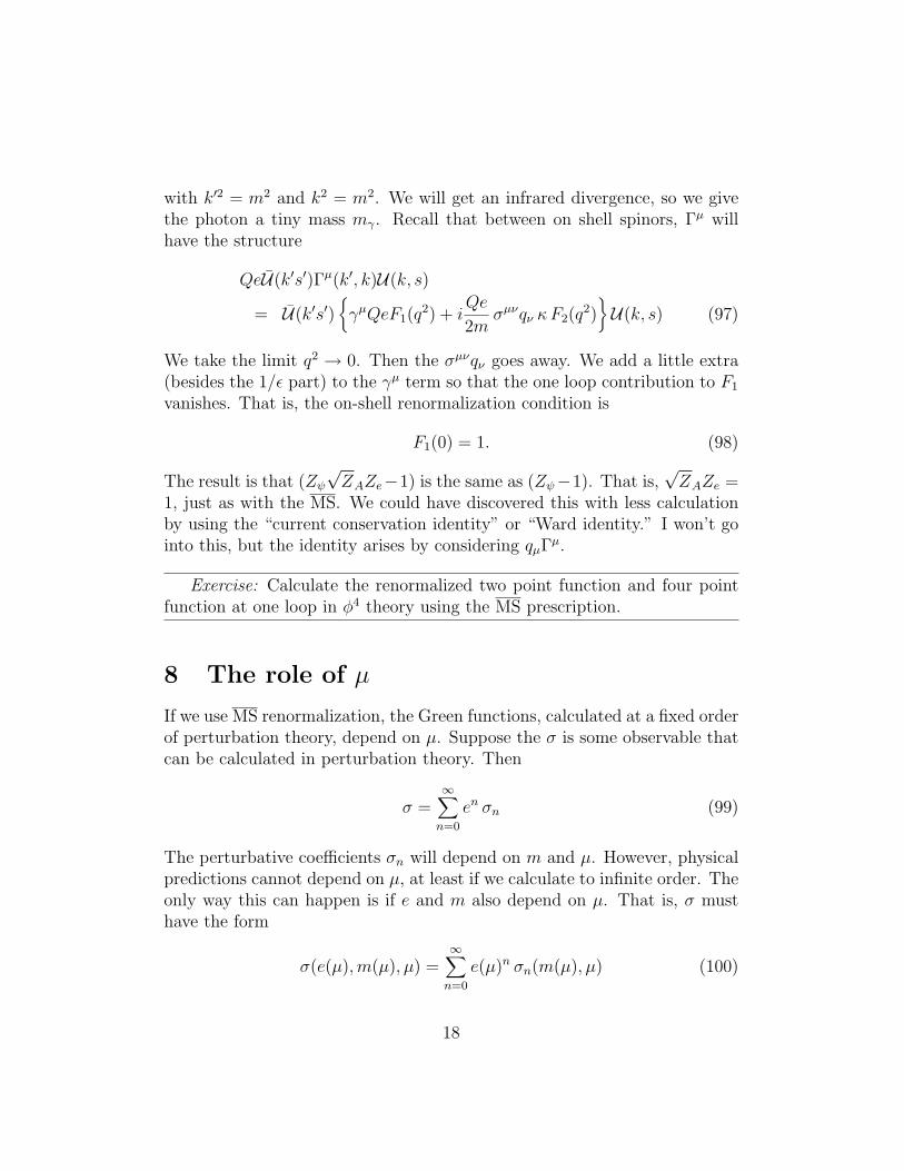
with k′2 = m2 and k2 = m2. We will get an infrared divergence, so we givethe photon a tiny mass mγ. Recall that between on shell spinors, Γµ willhave the structure

QeU(k′s′)Γµ(k′, k)U(k, s)

= U(k′s′)γµQeF1(q

2) + iQe

2mσµνqν κF2(q

2)U(k, s) (97)

We take the limit q2 → 0. Then the σµνqν goes away. We add a little extra(besides the 1/ε part) to the γµ term so that the one loop contribution to F1

vanishes. That is, the on-shell renormalization condition is

F1(0) = 1. (98)

The result is that (Zψ√ZAZe−1) is the same as (Zψ−1). That is,

√ZAZe =

1, just as with the MS. We could have discovered this with less calculationby using the “current conservation identity” or “Ward identity.” I won’t gointo this, but the identity arises by considering qµΓ

µ.

Exercise: Calculate the renormalized two point function and four pointfunction at one loop in φ4 theory using the MS prescription.

8 The role of µ

If we use MS renormalization, the Green functions, calculated at a fixed orderof perturbation theory, depend on µ. Suppose the σ is some observable thatcan be calculated in perturbation theory. Then

σ =∞∑n=0

en σn (99)

The perturbative coefficients σn will depend on m and µ. However, physicalpredictions cannot depend on µ, at least if we calculate to infinite order. Theonly way this can happen is if e and m also depend on µ. That is, σ musthave the form

σ(e(µ),m(µ), µ) =∞∑n=0

e(µ)n σn(m(µ), µ) (100)

18

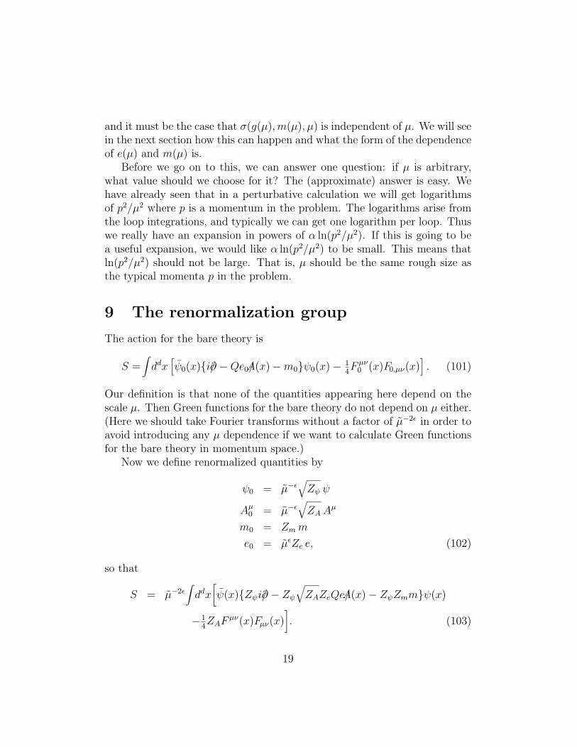
and it must be the case that σ(g(µ),m(µ), µ) is independent of µ. We will seein the next section how this can happen and what the form of the dependenceof e(µ) and m(µ) is.

Before we go on to this, we can answer one question: if µ is arbitrary,what value should we choose for it? The (approximate) answer is easy. Wehave already seen that in a perturbative calculation we will get logarithmsof p2/µ2 where p is a momentum in the problem. The logarithms arise fromthe loop integrations, and typically we can get one logarithm per loop. Thuswe really have an expansion in powers of α ln(p2/µ2). If this is going to bea useful expansion, we would like α ln(p2/µ2) to be small. This means thatln(p2/µ2) should not be large. That is, µ should be the same rough size asthe typical momenta p in the problem.

9 The renormalization group

The action for the bare theory is

S =∫ddx

[ψ0(x)i/∂ −Qe0/A(x)−m0ψ0(x)− 1

4F µν

0 (x)F0,µν(x)]. (101)

Our definition is that none of the quantities appearing here depend on thescale µ. Then Green functions for the bare theory do not depend on µ either.(Here we should take Fourier transforms without a factor of µ−2ε in order toavoid introducing any µ dependence if we want to calculate Green functionsfor the bare theory in momentum space.)

Now we define renormalized quantities by

ψ0 = µ−ε√Zψ ψ

Aµ0 = µ−ε√ZAA

µ

m0 = Zmm

e0 = µεZe e, (102)

so that

S = µ−2ε∫ddx

[ψ(x)Zψi/∂ − Zψ

√ZAZeQe/A(x)− ZψZmmψ(x)

−14ZAF

µν(x)Fµν(x)]. (103)

19

Consider the dimensionality of the various quantities that appear in the ac-tion. The quantities ψ0, A

µ0 ,m0, e0 have dimensions

(mass)3/2−ε, (mass)1−ε, (mass)1, (mass)ε. (104)

The functions Z are, by defintion, dimensionless. Thus we have defined therenormalized quantities ψ,Aµ,m, e so that they have dimension

(mass)3/2, (mass)1, (mass)1, (mass)0. (105)

With MS renormalization, the Zs depend only on the the renormalizedcoupling g but not separately on µ/m.(We have seen this at least at firstorder). But g0 does not depend on µ. Thus the only way that e0 = µεZg e,can hold is that e depends on µ. Similarly m must depend on µ. I argued inthe preceeding section that the requirement that physical observables mustbe independent of µ requires that e and m must depend on µ. The easy wayto see how e and m depend on µ is to use the fact that the bare theory doesnot have any µ dependence and use “the bare quantities are independent ofµ” instead of “physical observables are independent of µ.”

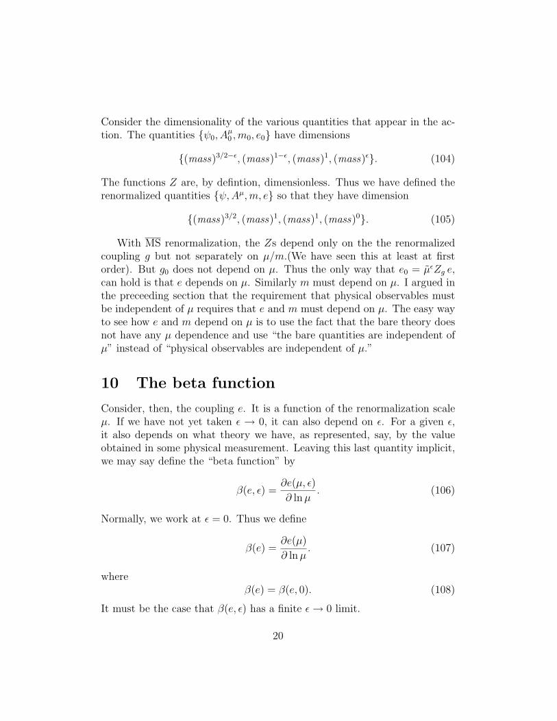
10 The beta function

Consider, then, the coupling e. It is a function of the renormalization scaleµ. If we have not yet taken ε → 0, it can also depend on ε. For a given ε,it also depends on what theory we have, as represented, say, by the valueobtained in some physical measurement. Leaving this last quantity implicit,we may say define the “beta function” by

β(e, ε) =∂e(µ, ε)

∂ lnµ. (106)

Normally, we work at ε = 0. Thus we define

β(e) =∂e(µ)

∂ lnµ. (107)

whereβ(e) = β(e, 0). (108)

It must be the case that β(e, ε) has a finite ε→ 0 limit.

20

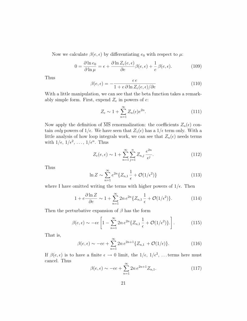
Now we calculate β(e, ε) by differentiating e0 with respect to µ:

0 =∂ ln e0∂ lnµ

= ε+∂ lnZe(e, ε)

∂eβ(e, ε) +

1

eβ(e, ε). (109)

Thusβ(e, ε) = − ε e

1 + e ∂ lnZe(e, ε)/∂e(110)

With a little manipulation, we can see that the beta function takes a remark-ably simple form. First, expend Ze in powers of e:

Ze ∼ 1 +∞∑n=1

Zn(ε)e2n. (111)

Now apply the definition of MS renormalization: the coefficients Zn(ε) con-tain only powers of 1/ε. We have seen that Z1(ε) has a 1/ε term only. With alittle analysis of how loop integrals work, we can see that Zn(ε) needs termswith 1/ε, 1/ε2, . . . , 1/εn. Thus

Ze(e, ε) ∼ 1 +∞∑n=1

n∑j=1

Zn,je2n

εj. (112)

Thus

lnZ ∼∞∑n=1

e2nZn,11

ε+O(1/ε2) (113)

where I have omitted writing the terms with higher powers of 1/ε. Then

1 + e∂ lnZ

∂e∼ 1 +

∞∑n=1

2n e2nZn,11

ε+O(1/ε2). (114)

Then the perturbative expansion of β has the form

β(e, ε) ∼ −εe[1−

∞∑n=1

2n e2nZn,11

ε+O(1/ε2).

]. (115)

That is,

β(e, ε) ∼ −εe+∞∑n=1

2n e2n+1Zn,1 +O(1/ε). (116)

If β(e, ε) is to have a finite ε → 0 limit, the 1/ε, 1/ε2, . . . terms here mustcancel. Thus

β(e, ε) ∼ −εe+∞∑n=1

2n e2n+1Zn,1. (117)

21

and

β(e) ∼∞∑n=1

2n e2n+1Zn,1. (118)

That is to say, the coefficient of e2n+1 in the expansion of β(e) is obtainedby calculating the 1/ε term in Zn(ε) and multiplying by 2n.

11 The running coupling

Before going on to more about the renormalization group, let’s look at thebehavior of the running coupling.

Consider first the case ε > 0. Then for e2 1 we have the approximateequation

∂e(µ, ε)

∂ lnµ= −εe. (119)

The solution of this with a boundary condition at µ0 is

e(µ, ε) = e(µ0, ε) exp(−ε ln(µ/µ0)). (120)

That ise(µ, ε) = e(µ0, ε)(µ/µ0)

−ε. (121)

As the scale µ increases, the coupling decreases like a power of µ. We saythat the renormalization group has an ultraviolet-stable fixed point at e = 0.

A similar situation could occur at ε = 0 if the beta function has a zero atsome point e?. That is, suppose that β(e?) = 0 and

β(e) = β0 (e− e?) +O((e− e?)2) (122)

Then if e(µ) ≈ e? we have, approximately,

∂e(µ)

∂ lnµ= β0 (e(µ)− e?). (123)

The solution of this is

e(µ) = e? + [e(µ0)− e?]

(µ

µ0

)β0

. (124)

If β0 > 0, we have an ultraviolet-stable fixed point at e = e?. The couplingis driven to e? as µ increases. It approaches e? like a power of µ. If β0 < 0,

22

then the coupling is driven away from e? as µ increases and as soon as itgets far away we need to include a more accurate representation of the betafunction. In this case, we have in infrared stable fixed point. The couplingis driven to e? as µ increases. It approaches e? like a power of 1/µ.

Now, let’s consider the real case at ε = 0 in quantum electrodynamics.There

β(e) = 2e3Z(e)1,1 + · · · = +

1

3

e3

4π2+O(e5) (125)

We have the approximate renormalization group equation

de(µ)

d lnµ= β1 e(µ)3. (126)

with β1 = 1/(12π2). The solution of this is

e(µ)2 =e(µ0)

2

1− β1 e(µ0)2 ln(µ2/µ20). (127)

We might rewrite this as

α(µ)2 =α(µ0)

1− (α(µ0)/(3π)) ln(µ2/µ20). (128)

We have an infrared stable fixed point at e = 0. As µ decreases, e(µ) goesto zero. It goes to zero slowly, proportionally to 1/ ln(µ2).

As µ increases, e(µ) increases. If µ gets to be very large, we need moreterms in the beta function and the form of the solution given above is nolonger valid. In particular, there is an apparent pole in the solution above ifwe go to very large µ, but the existence of such a pole is not to be believedbecause it arises from solving an approximation to the renormalization groupequation outside the region of validity of the approximation.

It is worth noting that in quantum chromodynamics we have the samesituation, except that β1 < 0. Thus zero coupling is an ultraviolet stablefixed point. The effective coupling αs(µ) is large for µ ∼ 100 MeV. But theαs(µ) becomes small for large µ, with αs(100 GeV) ≈ 0.1.

12 Mass and field strength renormalization

The mass parameter in the lagrangian also depends on the scale µ. We have

m(µ, ε) = Zm(e(µ, ε), ε)−1m0 (129)

23

so∂ lnm(µ, ε)

∂ lnµ= γm(e, ε) (130)

where

γm(e, ε) = −∂ lnZm(e(µ), ε)

∂eβ(e, ε). (131)

Let

Zm(e, ε) ∼ 1 +∞∑n=1

n∑j=1

Z(m)n,j

e2n

εj. (132)

Then

lnZm ∼∞∑n=1

e2nZ(m)n,1

1

ε+O(1/ε2) (133)

and

γm(e, ε) = −∞∑n=1

2n e2n−1Z(m)n,1

1

ε+O(1/ε2) [−εe+ β(e)].

=∞∑n=1

2n e2nZ(m)n,1 +O(1/ε) (134)

The function γm(e, ε) has to have a finite ε → 0 limit, so the 1/ε termsmust cancel. Thus γm(e, ε) is independent of ε and is given at each order ofperturbation theory by the 1/ε term in Zm:

γm(e, ε) = γm(e) =∞∑n=1

2n e2nZ(m)n,1 . (135)

Let’s also look at the field strength renormalization at this time. We have

ψ = µεZψ(e(µ, ε), ε)−1/2 ψ0 (136)

with a similar equation for the field Aµ. To find out how anything with afactor of ψ changes when we change µ, we will need

γψ(e, ε) ≡ − ∂

∂ lnµln(µεZψ(e(µ, ε), ε)−1/2

)(137)

That is

γψ(e, ε) = −ε+1

2

∂ lnZψ(e(µ), ε)

∂eβ(e, ε). (138)

24

As before, we let

Zψ(e, ε) ∼ 1 +∞∑n=1

n∑j=1

Z(ψ)n,j

e2n

εj. (139)

Then

γψ(e, ε) = −ε+1

2

∞∑n=1

2n e2n−1Z(ψ)n,1

1

ε+O(1/ε2) [−εe+ β(e)].

= −ε−∞∑n=1

n e2nZ(ψ)n,1 +O(1/ε) (140)

The function γψ(e, ε) has to have a finite ε→ 0 limit, so the 1/ε terms mustcancel. Thus γψ(e, ε) has a term +ε plus an ε independent part:

γψ(e, ε) = −ε+ γψ(e) (141)

The ε independent γψ(e) is given at each order of perturbation theory by the1/ε term in Zψ:

γψ(e) = −∞∑n=1

n e2nZ(ψ)n,1 . (142)

Similarly γA(e, ε) = ε+ γA(e) with

γA(e) = −∞∑n=1

n e2nZ(A)n,1 . (143)

13 The running mass

We have seen that∂ lnm(µ)

∂ lnµ= γm(e(µ)). (144)

Let’s see what would happen if the coupling has an ultraviolet fixed point ate = e?. Then as µ increases, e(µ) approaches e? quite quickly, like a power.That means that (as soon as e is sufficiently near to e?, the equation for theevolution of m can be approximated by

∂ lnm(µ)

∂ lnµ= γm(e?). (145)

25

The solution of this is

m(µ) = m(µ0)

(µ

µ0

)γm. (146)

Thus m approaches either zero or infinity (depending on the sign of γm) witha power behavior.

In the real case of quantum electrodynamics, the physical coupling is nearto an infrared stable fixed point at e = 0. In this case, the behavior of m(µ)is quite different because γm approaches zero as e approaches the fixed point.We have

∂ lnm(µ)

∂ lnµ= γm(e(µ)).

∼ γ(1)m e(µ)2

∼ γ(1)m

(1/e(µ0)2)− 2β1 ln(µ/µ0)(147)

Our solution for the running coupling can be rewitten so that the equationbecomes

∂ lnm(µ)

∂ lnµ∼ − γ(1)

m

2β1 ln(µ/Λ)(148)

This step defines Λ as a measure of the size of the coupling. For quantumelectrodynamics, Λ is a very large mass scale, much bigger than any µ ofpractical interest. Thus ln(µ/Λ) is negative. The solution of this is

ln

(m(µ)

m(µ0)

)= −γ

(1)m

2β1

ln

(ln(µ/Λ)

ln(µ0/Λ)

). (149)

or

m(µ) = m(µ0)

(ln(µ/Λ)

ln(µ0/Λ)

)−γ(1)m /(2β1)

. (150)

Another way to write this is

m(µ) = m(µ0)

(e(µ0)

e(µ)

)−γ(1)m /β1

. (151)

Thus m(µ) varies slowly as µ changes, like a power of e(µ), which itselfdoesn’t change very quickly.

26

Recall that e doesn’t change quickly because the derivative of e withrespect to lnµ is proportional to e × e2 and e2 is small. It is instructiveto compare to the case of quantum chromodynamics. There β1 is negative,so that the coupling gets smaller as we go toward larger µ. But also, thecoupling is larger than in quantum electrodynamics. In fact, Λ is on theorder of 100 MeV. Here we can more clearly see the distinction between afixed point at a non-zero coupling and a fixed point a zero coupling. In thefirst case, m is proportional to a power of µ while in the second case m isproportional to a power of lnµ.

14 Renormalization group for Green functions

Consider a Green function written in coordinate space. We will try a threepoint eeγ Green function just for definiteness:

G(x1, x2, x3; e(µ),m(µ), µ) = 〈Ω|ψ(x1)ψ(x2)Aµ(x3)|Ω〉 (152)

How does this depend on µ? We have

G0(x1, x2, x3; e0,m0) = µ−3εZψ(e, ε)ZA(e, ε)1/2G(x1, x2, x3; e(µ),m(µ), µ)(153)

The bare Green function does not depend on µ. Therefore

0 =d

d lnµµ−3εZψ(e, ε)ZA(e, ε)1/2G(x1, x2, x3; e(µ),m(µ), µ) (154)

In taking the derivative, e0, m0, and ε are held fixed, but then e and m varyand we must differentiate the explicit µ dependence of G:

0 =

+2γψ(e, ε) + γA(e, ε) + β(e, ε)

∂

∂e+ γm(e)m

∂

∂m+

∂

∂ lnµ

×G(x1, x2, x3; e(µ),m(µ), µ) (155)

Taking the limit ε→ 0 this becomes

0 =

2γψ(e) + γA(e) + β(e)

∂

∂e+ γm(e)m

∂

∂m+

∂

∂ lnµ

×G(x1, x2, x3; e(µ),m(µ), µ). (156)

27

This was for a three-point function. In general, there is a γψ for each ψ or ψand a γA for each Aµ.

Exercise: For an observable quantity σ, we get the same equation withoutγψ and γA. Then the solution of the equation is

σ(e(µ),m(µ), µ) = σ(e(µ0),m(µ0), µ0) (157)

What is the solution with nonzero γψ and γA? (You can make appropriateapproximations).

15 Solution for amputated Green functions

Putting the renormalization group equation for Green functions into momen-tum space and applying it to amputated Green functions with nγ photon legsand nψ quark or antiquark legs, we have

0 =

µ∂

∂µ+ β(e)

∂

∂e+ γm(e)m

∂

∂m− nψγψ(e)− nAγA(e)

×G(p1, . . . , pN ; e(µ),m(µ), µ). (158)

(The signs of the γψ and γA terms gets reversed because we are consideringthe amputated Green functions. This happens because we have to divide bya two point function for each external leg to amputate it.) The solution is

G(p1, . . . , pN ; e(µ),m(µ), µ) = exp

(∫ µ

µ0

dµ

µ[nψγψ(e(µ)) + nAγA(e(µ))]

)×G(p1, . . . , pN ; e(µ0),m(µ0), µ0) (159)

This is without approximation. We can rewrite a factor like

exp

(∫ µ

µ0

dµ

µnγ(e(µ))

)(160)

approximately by expanding the objects involved to lowest order in pertur-bation theory. Let us adopt the notation

γ(e) = γ1α+ · · · (161)

28

anddα(µ)

d lnµ≡ β(α) = β1α

2 + · · · (162)

Then we have

exp

(∫ µ

µ0

dµ

µnγ(e(µ))

)= exp

(∫ µ

µ0

dµ

µnγ1α(µ)

)

= exp

(∫ α(µ)

α(µ0)

dα

β1α2nγ1α

)

= exp

(γ1

β1

∫ α(µ)

α(µ0)

dα

α

)

= exp

(nγ1

β1

ln

(α(µ)

α(µ0)

))

=

(α(µ)

α(µ0)

)nγ1/β1

(163)

This is essentially the same result that we derived for m(µ) in a slightlydifferent way. In a theory that has a fixed point at a non-zero value of thecoupling, we would have a power of µ. In the case of QED, we get a powerof a constant plus ln(µ).

16 Application of the R-G equation

Now I would like to apply the renormalization group equation to the fol-lowing physical problem. We consider an amputated Green function withexternal momenta pν1, . . . , p

νn. (We could consier other quantities that are

made by multiplying or dividing Green functions by one another, but a sim-ple amputeated Green function will serve as a good example.) We can startwith the momenta all of order some reference scale µ0. (For particle physics,µ0 might be the mass of the Z boson. For field theory models in condensedmatter physics, the reference momentum scale might be an inverse nanome-ter.) Now we ask what happens when we scale all of the momenta by a largefactor, either toward the infrared or the ultraviolet. That is, we take

pνi ∼ µ (164)

where µ µ0 or else µ µ0. We ask how

G(p1, . . . , pn; e(µ0),m(µ0), µ0) (165)

29

behaves as we change the scale of the pν1i . Note that we are keeping thetheory absolutely fixed here: we have arguments e(µ0),m(µ0), µ0 of G.

We can use the renormalization group to help us. We know that we sholdnot calculate with a renormalization scale µ0 if the momentum scale is verydifferent. Therefore, let’s change the renormalization scale to µ. We have

G(p1, . . . , pn; e(µ0),m(µ0), µ0) =

exp

(−∫ µ

µ0

dµ

µ[nψγψ(e(µ)) + nAγA(e(µ))]

)×G(p1, . . . , pn; e(µ),m(µ), µ) (166)

Now we can apply dimensional analysis. I claim that the dimension of Gis

dG = 4− nA − 3nψ/2. (167)

We can prove this later. For the moment, let’s just apply it. We have

G(p1, . . . , pn; e(µ),m(µ), µ) =

µ4−nA−3nψ/2 G(p1/µ, . . . , pn/µ; e(µ),m(µ)/µ, 1) (168)

On the right hand side, we have G a dimensionless function of dimensionlessvariables times a factor µdG that carries the dimension. Then

G(p1, . . . , pn; e(µ0),m(µ0), µ0) =

exp

(−∫ µ

µ0

dµ

µ

nψ[3/2 + γψ(e(µ))] + nA[1 + γA(e(µ))]

)×(µ/µ0)

4µ4−nA−3nψ/20 G(p1/µ, . . . , pn/µ; e(µ),m(µ)/µ, 1). (169)

What lessons do we learn. First, there is a factor (µ/µ0)−nA−3nψ/2 that

comes from the dimensionalities 3/2 and 1 of the fields ψ and Aν respectively.I have put these into the integral in the exponential. We see that the 3/2 getschanged to 3/2 + γψ. For this reason, we call γψ the anomalous dimension ofψ. Similarly the 1 gets changed to 1 + γA, so that we call γA the anomalousdimension of Aν . Thus the scaling that we might have expected because ofthe dimensions of the field operators gets modified by loop graphs. Second, arather trivial scale dependent factor remains (µ/µ0)

4 because there is a term

“4” in the dimension of G. Third, there is a fixed factor µ4−nA−3nψ/20 that

carries the dimensions of G. Finally, there is a dimensionless factor

G(p1/µ, . . . , pn/µ; e(µ),m(µ)/µ, 1). (170)

30

Typically, this factor does not have any large logarithms in it, so a pertur-bative calculation should be OK as long as e(µ) is small. This factor does,however, depend on µ even when we hold the pνi /µ fixed. That is becausethe dimensionless parameters e(µ) and m(µ)/µ change with µ.

Exercise: Prove that the dimension of an amputated Green function inQED with nψ electron or positron legs and nA photon legs is dG = 4− nA −3nψ/2. Hint: First consider tree diagrams and just count the dimensionscoming from the Feynman rules. Next, show that adding any number ofloops does not change the dimensionality of a graph.

17 Renormalization group flows

We see that aside from the exponential factor, our amputated Green functionis controlled by the function

G(p1/µ, . . . , pn/µ; e(µ),m(µ)/µ, 1). (171)

where we are supposing that all of the pν1 are of the same order and we havechosen µ to be of this order. What happens if we start out with a big µ(say 100 GeV) and move toward smaller values of µ? Then e(µ) and m(µ)/µchange according to

∆e = −β(e) ∆ln(1/µ)

∆

(m

µ

)= (1− γm(e))

(m

µ

)∆ln(1/µ). (172)

A convenient way to think about this is to make a plot of m/µ versus e and,for each point, to draw a little arrow indicating how m/µ and e change as µdecreases. The arrows are tangent to the actual paths m(µ)/µ, e(µ). Therecould be different paths with the arrows as their tangents that correspond todifferent versions of QED. (That is, different paths correspond to differentvalues of the physical electron mass and fine structure constant.)

What this picture shows is that, at least in the small e region, e decreases(slowly) as we move toward the infrared, while m/µ increases. As long asm/µ is small, its rate of increase is small, but as it becomes larger its rate ofincrease becomes larger. It is the “1” in (1− γm(e)) that is important here.The 1 corresponds to the 1/µ in m/µ. We are learning that for large µ, the

31

dimensionless parameter m/µ is small. In this case we can replace it by 0 inEq. (171). But if we decrease µ until it is of order m, then we can’t neglect mand the theory changes character. For m(µ)/µ 1 we are in a scaling regimein which the exponential factor in Eq. (169) is controlling the behavior of theGreen function on the left hand side while G(p1/µ, . . . , pn/µ; e(µ),m(µ)/µ, 1)changes only slowly. But when we reach m(µ)/µ ∼ 1, this behavior changescompletely. (There are analogies in condensed matter physics. See Peskinand Schroeder.)

In order to see what happens in a more complicated situation, considerthe following problem.

Exercise: Suppose that we add to the lagrangian for QED a term

∆L =λ

M2(ψψ)2. (173)

I write the coupling as λ/M2 in order to emphasize that it has dimension1/mass2. There is a contribution to the eeγ amputated Green function atone loop, order λe/M2. Calculate (using dimensional regularization) thedivergent part of this graph and thus determine the nature of the counter-terms necessary to renormalize it.

18 Adding more operators to the lagrangian

Let’s see what happens if we add more terms to the lagrangian. In the baretheory, let the added terms have the form

∆L =∑i

λ(0)i

MdiO(0)i (174)

where the operators are made from products of the fields and their derivativesor factors of m. For example

(ψψ)2, m ψ[γµ, γν ]ψFµν , ψγµψ (∂νFµν) (175)

(We count all factors of m as part of the operators as a technical trick to aidin counting dimensions in the analysis that follows.) In the starting version,Eq. (174), we should take all of the operators to be the bare versions. We

32

write the couplings in the form λ(0)i /Mdi in order to display the dimension-

ality:

di =3

2ni(ψ) + ni(A)− 4 (176)

where ni(ψ) is the number of ψ or ψ fields in Oi and ni(A) the number of A

fields. This makes the λ(0)i dimensionless in 4 space-time dimensions. Then

M is some convenient reference mass.Now we need to renormalize. For this purpose, let

O(0)i = (µ)−[ni(ψ)+ni(A)]εZ

ni(ψ)/2ψ Z

ni(A)/2A Oi. (177)

and letλ

(0)i = (µ)niε [λi + ∆i(e, λ)] (178)

whereni = [ni(ψ) + ni(A)− 2] (179)

and where the functions ∆i(e, λ) depend on e and all of the λj. Then

∫d4−2εx ∆L = µ2ε

∫d4−2εx

∑i

λiMdi

Oi

+∑i

λiMdi

[Zni(ψ)/2ψ Z

ni(A)/2A − 1]Oi

+∑i

∆i

MdiZni(ψ)/2ψ Z

ni(A)/2A Oi

. (180)

This gives us plenty of counter-terms, which we will define following the MSprescription.

The renormalization of the QED coupling e can be cast in this samescheme,

e(0) = (µ)neε [e+ ∆e(e, λ)] (181)

where ne = 1. Then we have countertermse[Zψ Z

1/2A − 1] + ∆e Zψ Z

1/2A

ψγµψAµ. (182)

The mass renormalization can remain in the same form as in our earlieranalysis, with

m0 = Zmm (183)

33

leading to counterterms

[Zψ Z1/2A Zm − 1] mψψ. (184)

Of particular interest is how the new couplings λi change when we changethe scale. We just modify our previous derivation for how e changes. Wedefine

β(e, λ, ε) =de(µ)

d lnµ

βi(e, λ, ε) =dλi(µ)

d lnµ(185)

Then

0 =∂ lnλ

(0)i

∂ lnµ

= niε+1

[λi + ∆i(e, λ)]

×

βi(e, λ, ε) +∂∆i(e, λ)

∂eβ(e, λ, ε) +

∑j

∂∆i(e, λ)

∂λjβj(e, λ, ε)

(186)

That is

−niε [λi+∆i(e, λ)] = βi(e, λ, ε)+∂∆i(e, λ)

∂eβ(e, λ, ε)+

∑j

∂∆i(e, λ)

∂λjβj(e, λ, ε)

(187)There is an equatin for the renormalization of e of the same structure. Justsubstitute λ0 = e. The corresponding dimension is n0 = 1.

Now we put in the structure of the counter terms:

∆i(e, λ) =1

ε∆

(1)i (e, λ) + · · · (188)

where the term displayed collects all of the terms in the perturbative expan-sion of ∆i(e, λ) that have factors of 1/ε while the + · · · indicates the otherterms, which have factors 1/ε2, 1/ε3, etc. We insist that the βi must have afinite limit as ε→ 0. Then the equation works if βi(e, λ, ε) has a single termproportional to ε plus an ε independent piece:

βi(e, λ, ε) = −niλiε+ βi(e, λ).

β(e, λ, ε) = −eε+ β(e, λ). (189)

34

With this ansatz, the terms proportional to ε in Eq. (187) match and theterms proportional to ε0 are

−ni∆(1)i (e, λ) = βi(e, λ)− ∂∆

(1)i (e, λ)

∂ee−

∑j

∂∆(1)i (e, λ)

∂λjnjλj (190)

That is

βi(e, λ) = −ni∆(1)i (e, λ) + e

∂∆(1)i (e, λ)

∂e+∑j

njλj∂∆

(1)i (e, λ)

∂λj. (191)

The equation for the beta function that controls the evolution of e is, simi-larly,

β(e, λ) = −∆(1)e (e, λ) + e

∂∆(1)e (e, λ)

∂e+∑j

njλj∂∆(1)

e (e, λ)

∂λj. (192)

If we leave out the third term on the right hand side, this is just the resultwe had before, simply written in a different way.

For the evolution of the mass, we have an equation that is the same asin our previous analysis except that one can allow, to begin with, that theanomalous dimension might depend on more variables:

∂ lnm(µ)

∂ lnµ= γm(e, λ) (193)

We get the anomalous dimension from the 1/ε parts of the countertermsusing

γm(e, λ) = e∂Z(1)

m (e, λ)

∂e+∑j

njλjZ(1)m (e, λ)

∂λj. (194)

Now let’s consider what terms can occur. In general ∆(1)i (e, λ) can have

a non-zero perturbative coefficient of

eN λn11 λn2

2 · · · (195)

ifdi = n1 d1 + n2 d2 + · · · . (196)

Otherwise the powers of M won’t match to create a counterterm for Oi.For the renormalization of e, we have de = 0, so the only contributions are

35

those with n1 = n2 = · · · = 0. That is, the new terms don’t affect therenormalization of e:

β(e, λ) = β(e). (197)

Similarly, if we expand Zm(e, λ) in powers of e and the λj, we can get anypower of e, but we cannot have powers of the λj. That is

γm(e, λ) = γm(e). (198)

In a way, this result is an accounting trick. A graph containing a highdimension term in ∆L can lead, for instance to the need for a counter termof the form (m3/M2)ψψ, but we count this as renormalizing the coefficientof the opoerator m3ψψ rather than as renormalizing the mass parameter.

Thus the new, high dimension terms do not change the renormalizationof the conventional QED terms. However, the new terms do affect the renor-malization of each other. And if we put just one new term with di > 0, we willneed an infinite number of terms. This makes the theory nonrenormalizable.We see that a nonrenormalizable theory has an infinite number of parametersλi. Thus people used to reject the possibility of having a nonrenormalizabletheory on the grounds that it has no predictive power.

However, a nonrenormalizable theory can be just fine if it is an effectivetheory that applies approximately at a momentum scale far below the scaleM of some ultimate theory. Then all of the λi can be not too large and theλi/M

di are very small.If we draw pictures of renormalization group flows, then we use dimen-

sionless couplings and find, in the language of K. Wilson,

• m(µ)/µ gets big as µ decreases. We call the corresponding operator,ψψ a relevant operator.

• e(µ) changes slowly as µ decreases. We call the corresponding operator,ψγµψAµ, a marginal operator. In the case of quantum electrodynam-ics, e(µ) gets slowly smaller as µ decreases. In the case of quantumelectrodynamics, the corresponding coupling g(µ) gets slowly larger asµ decreases.

• λi(µ)(µ/M)di gets small as µ decreases. We call the correspondingoperator, Oi, an irrelevant operator.

36