Quantum Electrodynamics - Welcome to SCIPPscipp.ucsc.edu/~dine/ph217/217_qed_perturbation_theory.pdf · Quantum Electrodynamics Physics 217 2013, Quantum Field Theory Michael Dine

Quantum Electrodynamics

Physics 217 2013, Quantum Field Theory

Michael DineDepartment of Physics

University of California, Santa Cruz

Nov. 2013

Physics 217 2013, Quantum Field Theory Quantum Electrodynamics

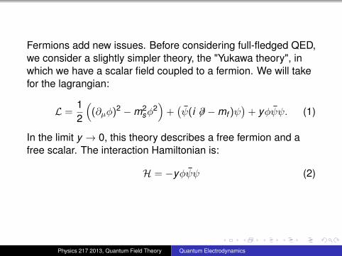
Fermions add new issues. Before considering full-fledged QED,we consider a slightly simpler theory, the "Yukawa theory", inwhich we have a scalar field coupled to a fermion. We will takefor the lagrangian:

L =12

((∂µφ)2 −m2

sφ2)

+(ψ(i 6∂ −mf )ψ

)+ yφψψ. (1)

In the limit y → 0, this theory describes a free fermion and afree scalar. The interaction Hamiltonian is:

H = −yφψψ (2)


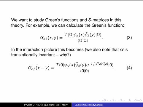
We want to study Green’s functions and S-matrices in thistheory. For example, we can calculate the Green’s function:

Gαβ(x , y) =T 〈Ω|ψα(x)ψβ(y)|Ω〉

〈Ω|Ω〉. (3)

In the interaction picture this becomes (we also note that G istranslationally invariant – why?)

Gαβ(x − y) =T 〈0|ψα(x)ψβ(y)e−i

∫d4zH(z)|0〉

〈0|0〉. (4)


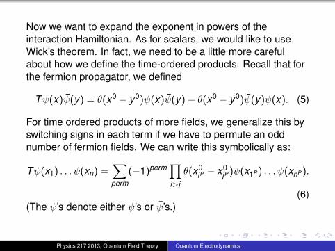
Now we want to expand the exponent in powers of theinteraction Hamiltonian. As for scalars, we would like to useWick’s theorem. In fact, we need to be a little more carefulabout how we define the time-ordered products. Recall that forthe fermion propagator, we defined

Tψ(x)ψ(y) = θ(x0 − y0)ψ(x)ψ(y)− θ(x0 − y0)ψ(y)ψ(x). (5)

For time ordered products of more fields, we generalize this byswitching signs in each term if we have to permute an oddnumber of fermion fields. We can write this symbolically as:

Tψ(x1) . . . ψ(xn) =∑perm

(−1)perm∏i>j

θ(x0iP − x0

jP )ψ(x1P ) . . . ψ(xnP ).

(6)(The ψ’s denote either ψ’s or ψ’s.)


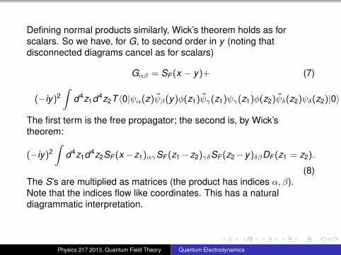
Defining normal products similarly, Wick’s theorem holds as forscalars. So we have, for G, to second order in y (noting thatdisconnected diagrams cancel as for scalars)

Gαβ = SF (x − y)+ (7)

(−iy)2∫

d4z1d4z2T 〈0|ψα(z)ψβ(y)φ(z1)ψγ(z1)ψγ(z1)φ(z2)ψδ(z2)ψδ(z2)|0〉

The first term is the free propagator; the second is, by Wick’stheorem:

(−iy)2∫

d4z1d4z2SF (x−z1)αγSF (z1−z2)γδSF (z2−y)δβDF (z1 = z2).

(8)The S’s are multiplied as matrices (the product has indices α, β).Note that the indices flow like coordinates. This has a naturaldiagrammatic interpretation.


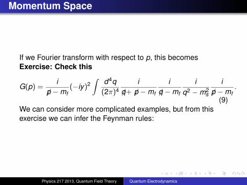
Momentum Space

If we Fourier transform with respect to p, this becomesExercise: Check this

G(p) =i

6p −mf(−iy)2

∫d4q

(2π)4i

6q+ 6p −mf

i6q −mf

iq2 −m2

s

i6p −mf

.

(9)We can consider more complicated examples, but from thisexercise we can infer the Feynman rules:


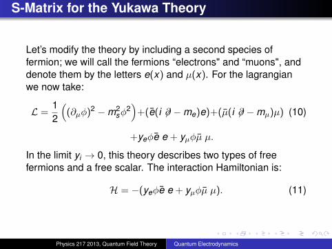
S-Matrix for the Yukawa Theory

Let’s modify the theory by including a second species offermion; we will call the fermions “electrons" and “muons", anddenote them by the letters e(x) and µ(x). For the lagrangianwe now take:

L =12

((∂µφ)2 −m2

sφ2)

+(e(i 6∂ −me)e)+(µ(i 6∂ −mµ)µ) (10)

+yeφe e + yµφµ µ.

In the limit yi → 0, this theory describes two types of freefermions and a free scalar. The interaction Hamiltonian is:

H = −(yeφe e + yµφµ µ). (11)


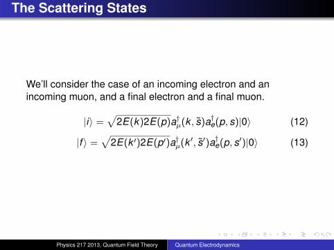
The Scattering States

We’ll consider the case of an incoming electron and anincoming muon, and a final electron and a final muon.

|i〉 =√

2E(k)2E(p)a†µ(k , s)a†e(p, s)|0〉 (12)

|f 〉 =√

2E(k ′)2E(p′)a†µ(k ′, s′)a†e(p, s′)|0〉 (13)


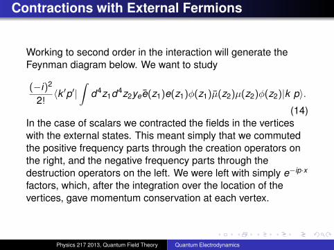
Contractions with External Fermions

Working to second order in the interaction will generate theFeynman diagram below. We want to study

(−i)2

2!〈k ′p′|

∫d4z1d4z2yee(z1)e(z1)φ(z1)µ(z2)µ(z2)φ(z2)|k p〉.

(14)In the case of scalars we contracted the fields in the verticeswith the external states. This meant simply that we commutedthe positive frequency parts through the creation operators onthe right, and the negative frequency parts through thedestruction operators on the left. We were left with simply e−ip·x

factors, which, after the integration over the location of thevertices, gave momentum conservation at each vertex.


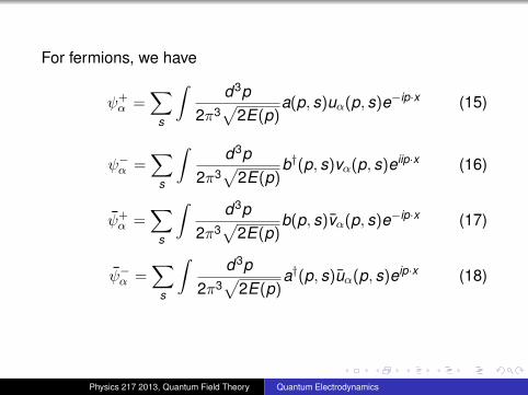
For fermions, we have

ψ+α =

∑s

∫d3p

2π3√

2E(p)a(p, s)uα(p, s)e−ip·x (15)

ψ−α =∑

s

∫d3p

2π3√

2E(p)b†(p, s)vα(p, s)eiip·x (16)

ψ+α =

∑s

∫d3p

2π3√

2E(p)b(p, s)vα(p, s)e−ip·x (17)

ψ−α =∑

s

∫d3p

2π3√

2E(p)a†(p, s)uα(p, s)eip·x (18)


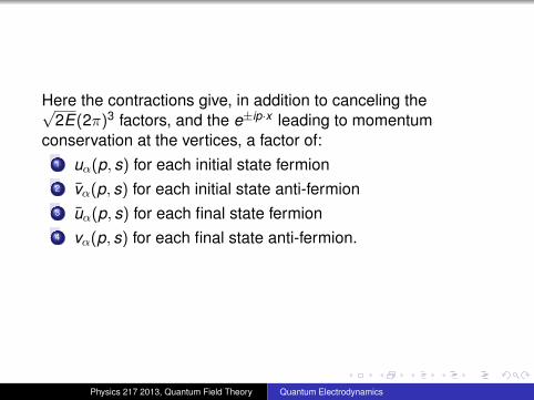
Here the contractions give, in addition to canceling the√2E(2π)3 factors, and the e±ip·x leading to momentum

conservation at the vertices, a factor of:1 uα(p, s) for each initial state fermion2 vα(p, s) for each initial state anti-fermion3 uα(p, s) for each final state fermion4 vα(p, s) for each final state anti-fermion.


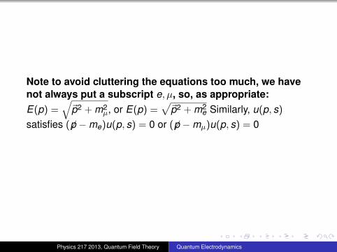
Note to avoid cluttering the equations too much, we havenot always put a subscript e, µ, so, as appropriate:E(p) =

√~p2 + m2

µ, or E(p) =√~p2 + m2

e Similarly, u(p, s)

satisfies ( 6p −me)u(p, s) = 0 or (6p −mµ)u(p, s) = 0


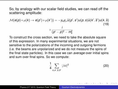
So, by analogy with our scalar field studies, we can read off thescattering amplitude:

M(e(p)+µ(k)→ e(p′)+µ(k ′)) = −yeyµu(p′, s′)u(p, s)u(k ′, s′)u(k , s)(19)

× i(p′ − p)2 −m2

s

To construct the cross section, we need to take the absolute squareof this expression. In many experimental situations, we are notsensitive to the polarizations of the incoming and outgoing fermions(i.e. the beams are unpolarized and we do not measure the spins ofthe final state particles). In this case we can average over initial spinsand sum over final spins. So we compute:

14

∑s,s′,s,s′

|M|2 (20)


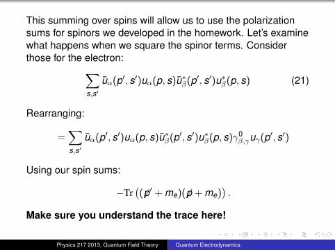
This summing over spins will allow us to use the polarizationsums for spinors we developed in the homework. Let’s examinewhat happens when we square the spinor terms. Considerthose for the electron:∑

s,s′uα(p′, s′)uα(p, s)u∗β(p′, s′)u∗β(p, s) (21)

Rearranging:

=∑s,s′

uα(p′, s′)uα(p, s)u∗β(p′, s′)u∗β(p, s)γ0β,γuγ(p′, s′)

Using our spin sums:

−Tr((6p′ + me)(6p + me)

).

Make sure you understand the trace here!


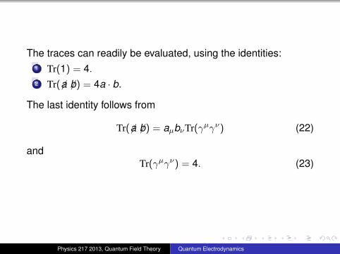
The traces can readily be evaluated, using the identities:1 Tr(1) = 4.2 Tr(6a 6b) = 4a · b.

The last identity follows from

Tr(6a 6b) = aµbνTr(γµγν) (22)

andTr(γµγν) = 4. (23)


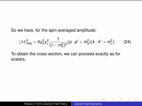
So we have, for the spin-averaged amplitude:

|M|2avg = 4y2e y2

µ

1(t −m2

s)2(p · p′ + m2

e)(k · k ′ + m2µ). (24)

To obtain the cross section, we can proceed exactly as forscalars,


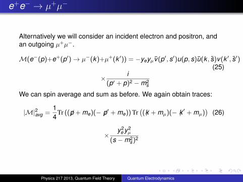
e+e− → µ+µ−

Alternatively we will consider an incident electron and positron, andan outgoing µ+µ−.

M(e−(p)+e+(p′)→ µ−(k)+µ+(k ′)) = −yeyµv(p′, s′)u(p, s)u(k , s)v(k ′, s′)(25)

× i(p′ + p)2 −m2

s

We can spin average and sum as before. We again obtain traces:

|M|2avg =14

Tr (( 6p + me)(− 6p′ + me)) Tr((6k + mµ)(− 6k ′ + mµ)

)(26)

×y2

e y2µ

(s −m2s )2


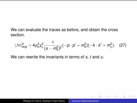
We can evaluate the traces as before, and obtain the crosssection.

|M|2avg = 4y2e y2

µ

1(s −m2

s)2(−p · p′ + m2

e)(−k · k ′ + m2µ). (27)

We can rewrite the invariants in terms of s, t and u.


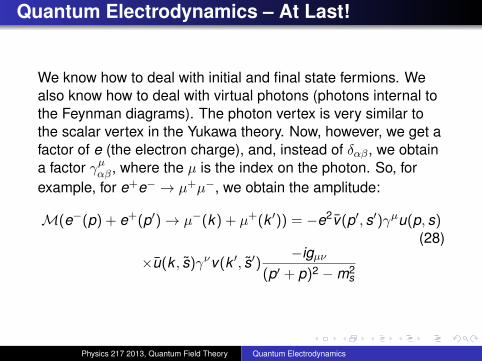
Quantum Electrodynamics – At Last!

We know how to deal with initial and final state fermions. Wealso know how to deal with virtual photons (photons internal tothe Feynman diagrams). The photon vertex is very similar tothe scalar vertex in the Yukawa theory. Now, however, we get afactor of e (the electron charge), and, instead of δαβ, we obtaina factor γµαβ, where the µ is the index on the photon. So, forexample, for e+e− → µ+µ−, we obtain the amplitude:

M(e−(p) + e+(p′)→ µ−(k) + µ+(k ′)) = −e2v(p′, s′)γµu(p, s)(28)

×u(k , s)γνv(k ′, s′)−igµν

(p′ + p)2 −m2s


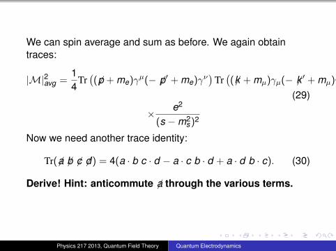
We can spin average and sum as before. We again obtaintraces:

|M|2avg =14

Tr((6p + me)γµ(− 6p′ + me)γν

)Tr((6k + mµ)γµ(− 6k ′ + mµ)γν

)(29)

× e2

(s −m2s)2

Now we need another trace identity:

Tr(6a 6b 6c 6d) = 4(a · b c · d − a · c b · d + a · d b · c). (30)

Derive! Hint: anticommute 6a through the various terms.


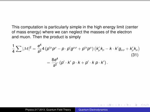
This computation is particularly simple in the high energy limit (centerof mass energy) where we can neglect the masses of the electronand muon. Then the product is simply

14

∑|M|2 =

e4

s2 4 (p′µpρ − p · p′gµρ + p′ρpµ)(k ′µkρ − k · k ′gµρ + k ′ρkµ

)(31)

=8e4

s2 (p′ · k ′ p · k + p′ · k p · k ′) .


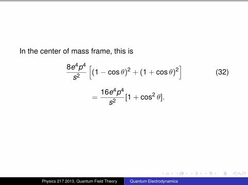
In the center of mass frame, this is

8e4p4

s2

[(1− cos θ)2 + (1 + cos θ)2

](32)

=16e4p4

s2 [1 + cos2 θ].


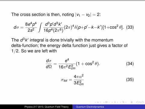
The cross section is then, noting |v1 − v2| = 2:

dσ =8e4p4

2s2

∫d3p′d3k ′

16p4(2π6)(2π)4δ(p+p′−k−k ′)[1+cos2 θ]. (33)

The d3k ′ integral is done trivially with the momentumdelta-function; the energy delta function just gives a factor of1/2. So we are left with

dσdΩ

=e4

16π2E2cm

(1 + cos2 θ). (34)

σtot =4πα2

3E2cm

(35)


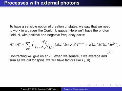
Processes with external photons

To have a sensible notion of creation of states, we saw that we needto work in a gauge like Coulomb gauge. Here we’ll have the photonfield, ~A, with positive and negative frequency parts:

A+i +A−i =

∑pol

∫d3p

(2π)3√

E(p)

(a(p, λ)εi (p, λ)e−ip·x + a†(p, λ)ε∗i (p, λ)eip·x) .

(36)Contracting will give us an εi . When we square, if we average andsum as we did for spins, we will have factors like Pij (~p).


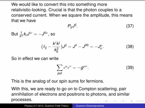
We would like to convert this into something morerelativistic-looking. Crucial is that the photon couples to aconserved current. When we square the amplitude, this meansthat we have

PijJ ij . (37)

But 1k0 kiJ iν = −J0ν , so

(δij −k ik j

k20

)J ij = J ii − J00 = −Jµµ . (38)

So in effect we can write∑pol

εµεν = −gµν . (39)

This is the analog of our spin sums for fermions.

With this, we are ready to go on to Compton scattering, pairannihilation of electrons and positrons to photons, and similarprocesses.


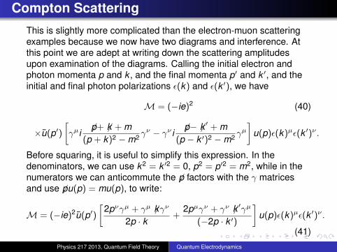
Compton Scattering

This is slightly more complicated than the electron-muon scatteringexamples because we now have two diagrams and interference. Atthis point we are adept at writing down the scattering amplitudesupon examination of the diagrams. Calling the initial electron andphoton momenta p and k , and the final momenta p′ and k ′, and theinitial and final photon polarizations ε(k) and ε(k ′), we have

M = (−ie)2 (40)

×u(p′)[γµi

6p+ 6k + m(p + k)2 −m2 γ

ν − γν i6p− 6k ′ + m

(p − k ′)2 −m2 γµ

]u(p)ε(k)µε(k ′)ν .

Before squaring, it is useful to simplify this expression. In thedenominators, we can use k2 = k ′2 = 0, p2 = p′2 = m2, while in thenumerators we can anticommute the 6p factors with the γ matricesand use 6pu(p) = mu(p), to write:

M = (−ie)2u(p′)[

2pνγµ + γµ 6kγν

2p · k+

2pµγν + γν 6k ′γµ

(−2p · k ′)

]u(p)ε(k)µε(k ′)ν .

(41)Physics 217 2013, Quantum Field Theory Quantum Electrodynamics

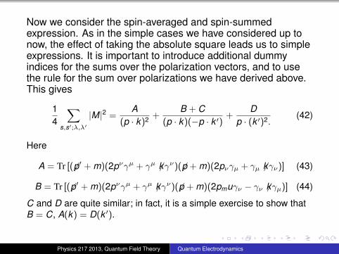
Now we consider the spin-averaged and spin-summedexpression. As in the simple cases we have considered up tonow, the effect of taking the absolute square leads us to simpleexpressions. It is important to introduce additional dummyindices for the sums over the polarization vectors, and to usethe rule for the sum over polarizations we have derived above.This gives

14

∑s,s′;λ,λ′

|M|2 =A

(p · k)2 +B + C

(p · k)(−p · k ′)+

Dp · (k ′)2.

(42)

Here

A = Tr [(6p′ + m)(2pνγµ + γµ 6kγν)( 6p + m)(2pνγµ + γµ 6kγν)] (43)

B = Tr [( 6p′ + m)(2pνγµ + γµ 6kγν)(6p + m)(2pmuγν − γν 6kγµ)] (44)

C and D are quite similar; in fact, it is a simple exercise to show thatB = C, A(k) = D(k ′).


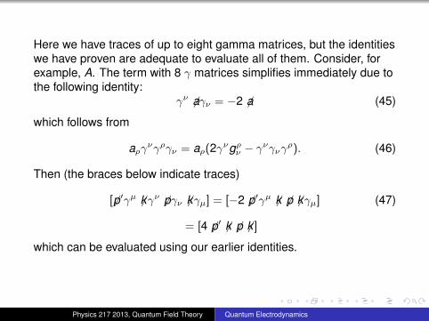
Here we have traces of up to eight gamma matrices, but the identitieswe have proven are adequate to evaluate all of them. Consider, forexample, A. The term with 8 γ matrices simplifies immediately due tothe following identity:

γν 6aγν = −2 6a (45)

which follows from

aργνγργν = aρ(2γνgρν − γνγνγρ). (46)

Then (the braces below indicate traces)

[6p′γµ 6kγν 6pγν 6kγµ] = [−2 6p′γµ 6k 6p 6kγµ] (47)

= [4 6p′ 6k 6p 6k ]

which can be evaluated using our earlier identities.


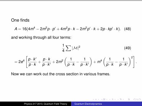
One finds

A = 16(4m4 − 2m2p · p′ + 4m2p · k − 2m2p′ · k + 2p · kp′ · k). (48)

and working through all four terms:

14

∑|M|2 (49)

= 2e4

[p · k ′

p · k+

p · kp · k ′

+ 2m2(

1p · k

− 1p · k ′

)+ m4

(1

p · k− 1

p · k ′

)2].

Now we can work out the cross section in various frames.


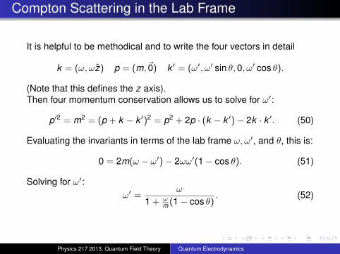
Compton Scattering in the Lab Frame

It is helpful to be methodical and to write the four vectors in detail

k = (ω, ωz) p = (m, ~0) k ′ = (ω′, ω′ sin θ,0, ω′ cos θ).

(Note that this defines the z axis).Then four momentum conservation allows us to solve for ω′:

p′2 = m2 = (p + k − k ′)2 = p2 + 2p · (k − k ′)− 2k · k ′. (50)

Evaluating the invariants in terms of the lab frame ω, ω′, and θ, this is:

0 = 2m(ω − ω′)− 2ωω′(1− cos θ). (51)

Solving for ω′:ω′ =

ω

1 + ωm (1− cos θ)

. (52)


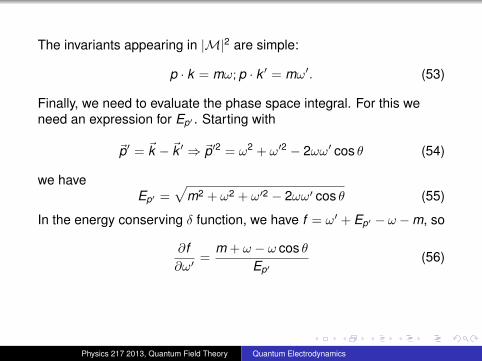
The invariants appearing in |M|2 are simple:

p · k = mω; p · k ′ = mω′. (53)

Finally, we need to evaluate the phase space integral. For this weneed an expression for Ep′ . Starting with

~p′ = ~k − ~k ′ ⇒ ~p′2 = ω2 + ω′2 − 2ωω′ cos θ (54)

we haveEp′ =

√m2 + ω2 + ω′2 − 2ωω′ cos θ (55)

In the energy conserving δ function, we have f = ω′ + Ep′ − ω −m, so

∂f∂ω′

=m + ω − ω cos θ

Ep′(56)


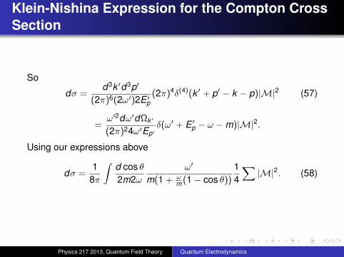
Klein-Nishina Expression for the Compton CrossSection

So

dσ =d3k ′d3p′

(2π)6(2ω′)2E ′p(2π)4δ(4)(k ′ + p′ − k − p)|M|2 (57)

=ω′2dω′dΩk ′

(2π)24ω′Ep′δ(ω′ + E ′p − ω −m)|M|2.

Using our expressions above

dσ =1

8π

∫d cos θ2m2ω

ω′

m(1 + ωm (1− cos θ))

14

∑|M|2. (58)


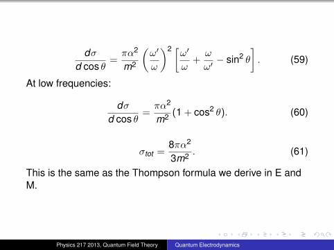
dσd cos θ

=πα2

m2

(ω′

ω

)2 [ω′ω

+ω

ω′− sin2 θ

]. (59)

At low frequencies:

dσd cos θ

=πα2

m2 (1 + cos2 θ). (60)

σtot =8πα2

3m2 . (61)

This is the same as the Thompson formula we derive in E andM.


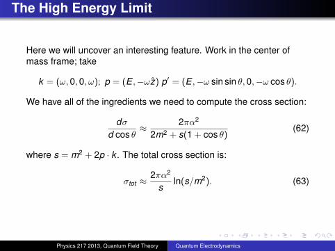
The High Energy Limit

Here we will uncover an interesting feature. Work in the center ofmass frame; take

k = (ω,0,0, ω); p = (E ,−ωz) p′ = (E ,−ω sin sin θ,0,−ω cos θ).

We have all of the ingredients we need to compute the cross section:

dσd cos θ

≈ 2πα2

2m2 + s(1 + cos θ)(62)

where s = m2 + 2p · k . The total cross section is:

σtot ≈2πα2

sln(s/m2). (63)


Colinear Singularities

Why the singularity as m→ 0. Should be able to see a problemif set m = 0 from the start problem comes when 2p · k or2p · k ′ = 0. Corresponds to p along k or k ′. The precise form ofthe singularity requires understanding the behavior of thespinors u(p) (see Peskin and Schroder).


Radiative Corrections

So far, we have considered “tree" diagrams; now we considerdiagrams with loops (in particular, this means diagrams whichhave an internal momentum integration). To perform theseintegrals, we will need to develop certain tools. We’ll do this inthe course of three examples which are particularly importantat one loop (e2 corrections to the leading order result). We’llalso have to face the problem of ultraviolet divergences (highmomentum). This will lead us to the problem ofrenormalization. Finally, we will face infrared divergences –these are associated with real physics.


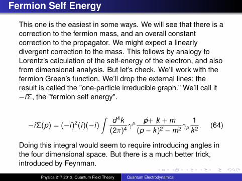
Fermion Self Energy

This one is the easiest in some ways. We will see that there is acorrection to the fermion mass, and an overall constantcorrection to the propagator. We might expect a linearlydivergent correction to the mass. This follows by analogy toLorentz’s calculation of the self-energy of the electron, and alsofrom dimensional analysis. But let’s check. We’ll work with thefermion Green’s function. We’ll drop the external lines; theresult is called the "one-particle irreducible graph." We’ll call it−iΣ, the "fermion self energy".

−iΣ(p) = (−i)2(i)(−i)∫

d4k(2π)4γ

µ 6p+ 6k + m(p − k)2 −m2γµ

1k2 . (64)

Doing this integral would seem to require introducing angles inthe four dimensional space. But there is a much better trick,introduced by Feynman.


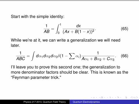
Start with the simple identity:

1AB

=

∫ 1

0

dx(Ax + B(1− x))2 . (65)

While we’re at it, we can write a generalization we will needlater.

1ABC

=

∫dα1dα2dα3δ(1−

∑αi)

1Aα1 + Bα2 + Cα3

. (66)

I’ll leave you to prove this second one; the generalization tomore denominator factors should be clear. This is known as the“Feynman parameter trick."


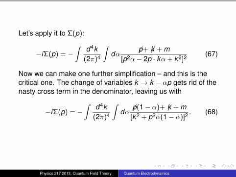
Let’s apply it to Σ(p):

−iΣ(p) = −∫

d4k(2π)4

∫dα

6p+ 6k + m[p2α− 2p · kα + k2]2

(67)

Now we can make one further simplification – and this is thecritical one. The change of variables k → k − αp gets rid of thenasty cross term in the denominator, leaving us with

−iΣ(p) = −∫

d4k(2π)4

∫dα6p(1− α)+ 6k + m

[k2 + p2α(1− α)]2. (68)


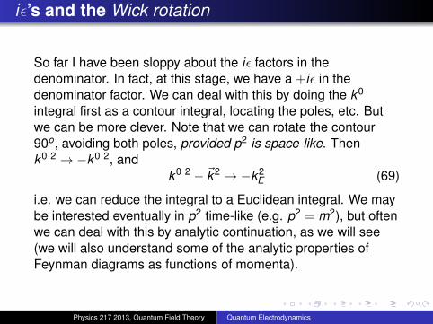
iε’s and the Wick rotation

So far I have been sloppy about the iε factors in thedenominator. In fact, at this stage, we have a +iε in thedenominator factor. We can deal with this by doing the k0

integral first as a contour integral, locating the poles, etc. Butwe can be more clever. Note that we can rotate the contour90o, avoiding both poles, provided p2 is space-like. Thenk0 2 → −k0 2, and

k0 2 − ~k2 → −k2E (69)

i.e. we can reduce the integral to a Euclidean integral. We maybe interested eventually in p2 time-like (e.g. p2 = m2), but oftenwe can deal with this by analytic continuation, as we will see(we will also understand some of the analytic properties ofFeynman diagrams as functions of momenta).


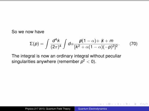
So we now have

Σ(p) =

∫d4k

(2π)4

∫dα

6p(1− α)+ 6k + m[k2 + α(1− α)(−p)2]2

. (70)

The integral is now an ordinary integral without peculiarsingularities anywhere (remember p2 < 0).


First simplification: the integral over the 6k term in the numeratoris odd, so gives zero.First complication: the integral is not well-defined. It diverges(logarithmically) for large k .This latter problem we might deal with as follows. We don’tknow about physics at arbitrarily large |k |. So we might justinclude all of the physics we know, and cut off the integralsabove that. Call that scale Λ; we might think of this as 100 TeV,or perhaps something larger. This is, in fact, what we will do.But we would like a way to cut off the integral so that the resultis simple and Lorentz invariant.


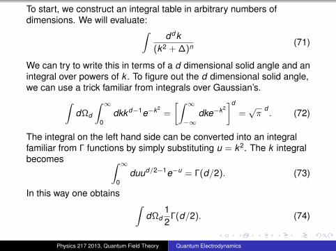
To start, we construct an integral table in arbitrary numbers ofdimensions. We will evaluate:∫

ddk(k2 + ∆)n (71)

We can try to write this in terms of a d dimensional solid angle and anintegral over powers of k . To figure out the d dimensional solid angle,we can use a trick familiar from integrals over Gaussian’s.∫

dΩd

∫ ∞0

dkkd−1e−k2=

[∫ ∞−∞

dke−k2]d

=√π

d. (72)

The integral on the left hand side can be converted into an integralfamiliar from Γ functions by simply substituting u = k2. The k integralbecomes ∫ ∞

0duud/2−1e−u = Γ(d/2). (73)

In this way one obtains ∫dΩd

12

Γ(d/2). (74)


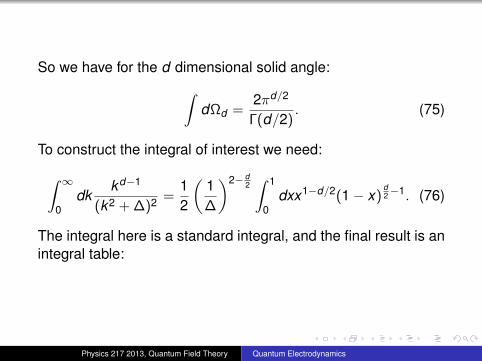
So we have for the d dimensional solid angle:∫dΩd =

2πd/2

Γ(d/2). (75)

To construct the integral of interest we need:∫ ∞0

dkkd−1

(k2 + ∆)2 =12

(1∆

)2− d2∫ 1

0dxx1−d/2(1− x)

d2−1. (76)

The integral here is a standard integral, and the final result is anintegral table:


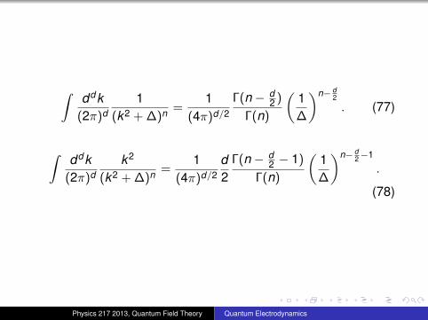
∫ddk

(2π)d1

(k2 + ∆)n =1

(4π)d/2

Γ(n − d2 )

Γ(n)

(1∆

)n− d2

. (77)

∫ddk

(2π)dk2

(k2 + ∆)n =1

(4π)d/2d2

Γ(n − d2 − 1)

Γ(n)

(1∆

)n− d2−1

.

(78)


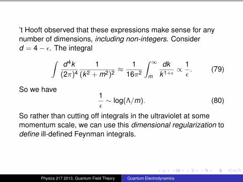
’t Hooft observed that these expressions make sense for anynumber of dimensions, including non-integers. Considerd = 4− ε. The integral∫

d4k(2π)4

1(k2 + m2)2 ≈

116π2

∫ ∞m

dkk1+ε ∝

1ε. (79)

So we have1ε∼ log(Λ/m). (80)

So rather than cutting off integrals in the ultraviolet at somemomentum scale, we can use this dimensional regularization todefine ill-defined Feynman integrals.


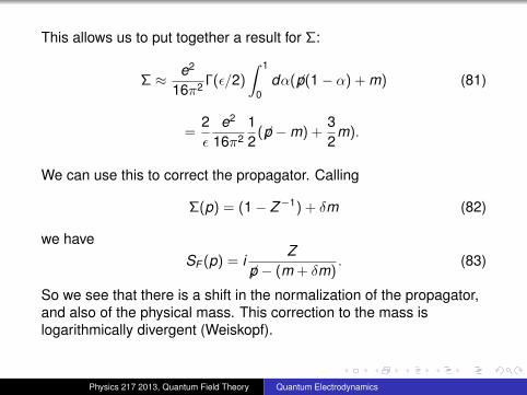
This allows us to put together a result for Σ:

Σ ≈ e2

16π2 Γ(ε/2)

∫ 1

0dα(6p(1− α) + m) (81)

=2ε

e2

16π212

( 6p −m) +32

m).

We can use this to correct the propagator. Calling

Σ(p) = (1− Z−1) + δm (82)

we haveSF (p) = i

Z6p − (m + δm)

. (83)

So we see that there is a shift in the normalization of the propagator,and also of the physical mass. This correction to the mass islogarithmically divergent (Weiskopf).


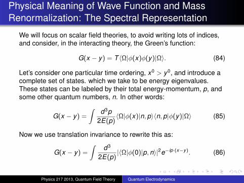
Physical Meaning of Wave Function and MassRenormalization: The Spectral Representation

We will focus on scalar field theories, to avoid writing lots of indices,and consider, in the interacting theory, the Green’s function:

G(x − y) = T 〈Ω|φ(x)φ(y)|Ω〉. (84)

Let’s consider one particular time ordering, x0 > y0, and introduce acomplete set of states. which we take to be energy eigenvalues.These states can be labeled by their total energy-momentum, p, andsome other quantum numbers, n. In other words:

G(x − y) =

∫d3p

2E(p)〈Ω|φ(x)|n,p〉〈n,p|φ(y)|Ω〉 (85)

Now we use translation invariance to rewrite this as:

G(x − y) =

∫d3

2E(p)|〈Ω|φ(0)|p,n〉|2e−ip·(x−y). (86)


Now we separate off states of definite mass(√

E(p)2 − p2 = M2). We define

ρ(M2) = δ(p2 −M2)|〈p,n|φ(0)|Ω〉|2. (87)

Then we have, including the other time ordering, and noting theconnection to the free propagator:

G(x − y) =

∫dM2ρ(M2)DF (x − y ; M). (88)

One can immediately Fourier transform this expression. Insimple field theories, ρ(M2) includes a δ function (at the massof the meson) and a continuum (e.g. starting at 9M2 in the caseof the φ4 theory).


One writes:

ρ(M2) = Zδ(M2 −m2) + fcont (M2). (89)

m2 is the actual mass of the physical state, by our construction.

This is known as the “spectral representation", or the"Kallen-Lehman representation".We can identify the Z and δm we have computed with thequantities here (to the order we have worked).


Renormalization

In δm, we have our first real example of the renormalization of aparameter. The observed, physical mass is m + δm. δm is“infinite" (depends on the cutoff, 1ε ∼ log(Λ), but we only careabout the observable quantity, the physical mass, and this is aparameter of the theory in any case (not something we canpredict). We will see that the electromagnetic coupling is alsorenormalized.

For this, we consider the corrections to the photon propagator,focussing on the one loop expressions. This is equivalent to

T 〈Ω|jµ(x)jν(y)|Ω〉 ≡ −iΠµν(q). (90)

(after Fourier transform).

The first thing to note is that since this involves conservedcurrents, we have

qµΠµν = 0. (91)


We can writeΠµν = (gµνq2 − qµqν)Π(q2) (92)

This makes the calculation easier; it is not hard to read off theqµqν piece.

To simplify the analysis, we will take q2 m2. Then writingdown the full diagram, it is not hard to pull out the qµqν pieces.


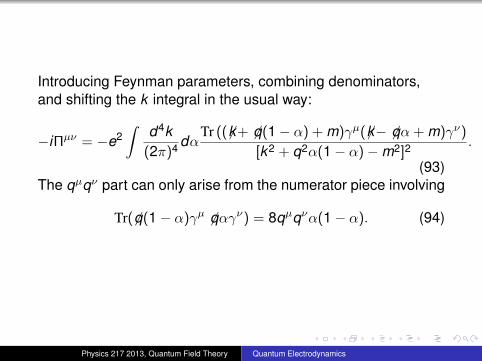
Introducing Feynman parameters, combining denominators,and shifting the k integral in the usual way:

−iΠµν = −e2∫

d4k(2π)4 dα

Tr ((6k+ 6q(1− α) + m)γµ(6k− 6qα + m)γν)

[k2 + q2α(1− α)−m2]2.

(93)The qµqν part can only arise from the numerator piece involving

Tr(6q(1− α)γµ 6qαγν) = 8qµqνα(1− α). (94)


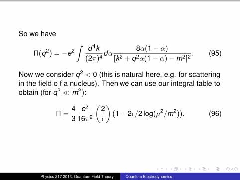
So we have

Π(q2) = −e2∫

d4k(2π)4 dα

8α(1− α)

[k2 + q2α(1− α)−m2]2. (95)

Now we consider q2 < 0 (this is natural here, e.g. for scatteringin the field o f a nucleus). Then we can use our integral table toobtain (for q2 m2):

Π =43

e2

16π2

(2ε

)(1− 2ε/2 log(µ2/m2)). (96)


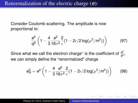
Renormalization of the electric charge (e):

Consider Coulomb scattering. The amplitude is nowproportional to:

e2

q2

(1− 4

3e2

16π22ε

(1− 2ε/2 log(µ2/m2))

)(97)

Since what we call the electron charge∗ is the coefficient of e2

q2 ,we can simply define the “renormalized" charge

e2R = e2

(1− 4

3e2

16π22ε

(1− 2ε/2 log(µ2/m2))

)(98)


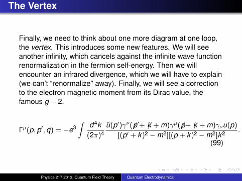
The Vertex

Finally, we need to think about one more diagram at one loop,the vertex. This introduces some new features. We will seeanother infinity, which cancels against the infinite wave functionrenormalization in the fermion self-energy. Then we willencounter an infrared divergence, which we will have to explain(we can’t “renormalize" away). Finally, we will see a correctionto the electron magnetic moment from its Dirac value, thefamous g − 2.

Γµ(p,p′,q) = −e3∫

d4k(2π)4

u(p′)γν( 6p′+ 6k + m)γµ( 6p+ 6k + m)γνu(p)

[(p′ + k)2 −m2][(p + k)2 −m2]k2 .

(99)


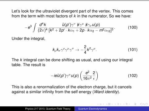
Let’s look for the ultraviolet divergent part of the vertex. This comesfrom the term with most factors of k in the numerator, So we have:

−e3∫

d4k(2π)4

u(p′)γν 6kγµ 6kγνu(p)

[k2 + 2p′ · kα1 + 2p · kα2 −m2α12]3. (100)

Under the integral,

kρkσγργµγσ → −24

k2γµ. (101)

The k integral can be done shifting as usual, and using our integraltable. The result is

−ieu(p′)γµu(p)

(e2

16π22ε

)(102)

This is also a renormalization of the electron charge, but it cancelsagainst a similar infinity from the self energy (Ward identity).


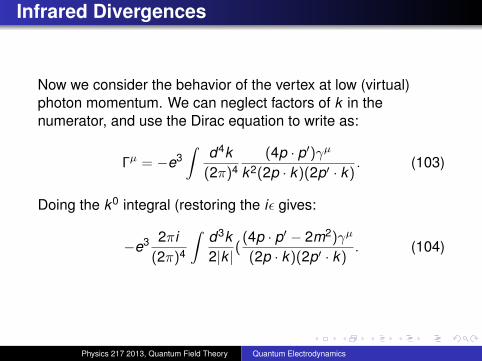
Infrared Divergences

Now we consider the behavior of the vertex at low (virtual)photon momentum. We can neglect factors of k in thenumerator, and use the Dirac equation to write as:

Γµ = −e3∫

d4k(2π)4

(4p · p′)γµ

k2(2p · k)(2p′ · k). (103)

Doing the k0 integral (restoring the iε gives:

−e3 2πi(2π)4

∫d3k2|k |

((4p · p′ − 2m2)γµ

(2p · k)(2p′ · k). (104)


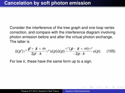
Cancelation by soft photon emission

Consider the interference of the tree graph and one loop vertexcorrection, and compare with the interference diagram involvingphoton emission before and after the virtual photon exchange.The latter is

u(p′)γν6p′+ 6k + m

2p′ · kγµu(p)u(p)

γν(6p− 6k + m)γρ

−2p · ku(p). (105)

For low k , these have the same form up to a sign.


Now no experiment can resolve photons of arbitrarily small ~k .So we can introduce an energy resolution, Er . The actualdivergence then cancels between the two diagrams, and we areleft with a result proportional to log(Er/E), where E is a typicalenergy scale in the process. For high energies, we also get alog of the mass, as we saw in Compton scattering, from theintegral over angles, The result is known as a “Sudakov doublelogarithm". There are actually such logs in every order ofperturbation theory, and it is possible to add up these largeterms (they exponentiate; see Peskin and Schroeder).


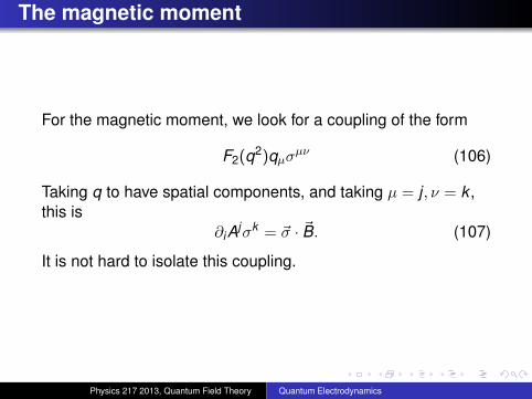
The magnetic moment

For the magnetic moment, we look for a coupling of the form

F2(q2)qµσµν (106)

Taking q to have spatial components, and taking µ = j , ν = k ,this is

∂iAjσk = ~σ · ~B. (107)

It is not hard to isolate this coupling.


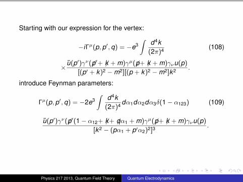
Starting with our expression for the vertex:

−iΓµ(p,p′,q) = −e3∫

d4k(2π)4 (108)

× u(p′)γν( 6p′+ 6k + m)γµ(6p+ 6k + m)γνu(p)

[(p′ + k)2 −m2][(p + k)2 −m2]k2 .

introduce Feynman parameters:

Γµ(p,p′,q) = −2e3∫

d4k(2π)4 dα1dα2dα3δ(1− α123) (109)

u(p′)γν( 6p′(1− α12+ 6k+ 6qα1 + m)γµ(6p+ 6k + m)γνu(p)

[k2 − (pα1 + p′α2)2]3.


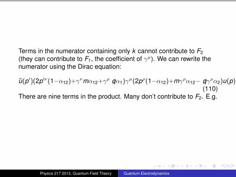
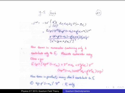
Terms in the numerator containing only k cannot contribute to F2(they can contribute to F1, the coefficient of γµ). We can rewrite thenumerator using the Dirac equation:

u(p′)(2p′ν(1−α12)+γνmα12+γρ 6qα1)γµ(2pρ(1−α12)+mγρα12− 6qγρα2)u(p).(110)

There are nine terms in the product. Many don’t contribute to F2. E.g.


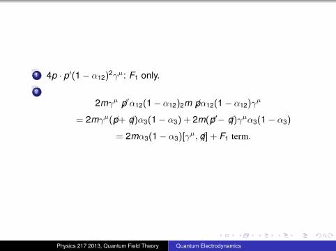
1 4p · p′(1− α12)2γµ: F1 only.

2

2mγµ 6p′α12(1− α12)2m 6pα12(1− α12)γµ

= 2mγµ(6p+ 6q)α3(1− α3) + 2m( 6p′− 6q)γµα3(1− α3)

= 2mα3(1− α3)[γµ, 6q] + F1 term.


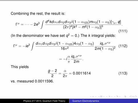
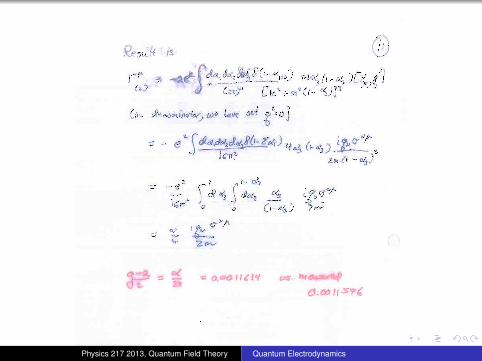
Combining the rest, the result is:

Γµ = · · · − 2e3∫

d4kdα1dα2dα3δ(1− α123)mα3(1− α3)[γµ, 6q]

(2π)4[k2 −m2(1− α3)]3.

(111)(In the denominator we have set q2 = 0.) The k integral yields:

Γµ = −ie3∫

dα1dα2dα3δ(1− α123)4α3(1− α3)

16π2iqνσνµ

2m(1− α3)2 (112)

= −iα

π

iqνσνµ

2m.

This yieldsg − 2

2=

α

2π= 0.0011614 (113)

vs. measured 0.0011596.




Documents

Quantum Electrodynamics - Welcome to SCIPPscipp.ucsc.edu/~dine/ph217/217_qed_perturbation_theory.pdf · Quantum Electrodynamics Physics 217 2013, Quantum Field Theory Michael Dine