Embed Size (px)
Citation preview

Faculdade de Engenharia da Universidade do Porto
Reliability Impact onHigh Penetration of Electric Vehicles
Master in Electrical and Computers Engineering
Supervisor: Prof. Dr. Vladimiro Henrique Barrosa Pinto de MirandaCo-Supervisor: Prof. Dr. Mauro Augusto da Rosa
Faculdade de Engenharia da Universidade do Porto
Reliability Impact on Power Systems Considering High Penetration of Electric Vehicles
Miguel Luís Delgado Heleno
Dissertation carried out under the Master in Electrical and Computers Engineering
Branch: Energy
Supervisor: Prof. Dr. Vladimiro Henrique Barrosa Pinto de MirandaSupervisor: Prof. Dr. Mauro Augusto da Rosa
June, 2010.
Faculdade de Engenharia da Universidade do Porto
Considering High Penetration of Electric Vehicles
Master in Electrical and Computers Engineering
Supervisor: Prof. Dr. Vladimiro Henrique Barrosa Pinto de Miranda Supervisor: Prof. Dr. Mauro Augusto da Rosa

© Miguel Luís Delgado Heleno, 2010

iii


v
“Ideas that enter the mind under fire remain there securely and forever.”
Leon Trotsky


vii
Abstract
In this work, some typical load diagrams including electric vehicles effects are studied, in
order to assess the security of supply of different generation systems. The scenarios are
exploring electric vehicles penetrations in six different European countries. Therefore, a
generation adequacy evaluation based on analytical calculation is proposed.
In fact, an analytical approach involving analytical calculation and simulation methods are
developed in order to perform the proposed evaluations. Some distinct approaches to
represent the chronological features of wind and other unconventional sources are compared.
The seasonal aspects of hydro reservoirs depletion is also considered through the affectation
of the capacities and the monthly evaluation of the indices. Then, a discussion about the
accuracy of the chosen methodology is done and the differences between this approach and a
flexible Sequential Monte Carlo Simulation are identified.
The methodology is applied to different test system, however, the modified Reliability
Test System 96 (IEEE-RTS 96) considering wind power and the mentioned electric vehicles
characteristic of the European countries is used. Two management concepts scenarios are
compared: smart charging and dumb charging. Furthermore, security of supply of the
Portuguese generation system is analyzed and the monthly and annual indices are obtained.


ix
Resumo
Neste trabalho, são estudadas alguns tipos de diagramas de carga, considerando os efeitos
da penetração de veículos eléctricos, no sentido de avaliar a segurança de abastecimento dos
sistemas produtores. Os cenários de penetração usados, característicos de seis países
europeus, são dados de entrada de uma ferramenta que, recorrendo a métodos analíticos,
visa fazer esse mesmo estudo.
Dado a complexidade dos sistemas de produção, para este tipo de estudos de fiabilidade
recorre-se por vezes a métodos híbridos, que utilizam concomitantemente cálculos analíticos
e métodos de simulação. Neste trabalho, são comparadas algumas abordagens para a
representação de fontes de energia com uma grande componente cronológica associada. A
flutuação sazonal dos níveis das albufeiras, obtida através dos índices mensais, é também
alvo de discussão neste documento. Após o desenvolvimento da metodologia analítica mais
adequada, esta é comparada com o método de Monte Carlo cronológico, a fim de identificar
as principais diferenças existentes entre eles.
O método analítico desenvolvido é depois aplicado ao sistema teste IEEE-RTS 96. No
entanto, algumas mudanças são feitas neste sistema, tendo em vista a inclusão tanto da
produção eólica como dos cenários de penetração de veículos eléctricos característicos dos
seis países europeus. Nestes cenários são estudados dois modelos de gestão da carga: smart
charging e dumb charging. Por fim é feita uma avaliação de segurança de abastecimento do
sistema português.


xi
Acknowledgements
First, I would like to thank to my supervisor, Professor Vladimiro Miranda, for the several
advices given in order to improve this Thesis. Then, I would like to express my gratitude to
Professor Roy Billinton, Professor Armando Martins Leite da Silva and his PhD student
Reinaldo, for the explanations during the implementation of the methods. I am also grateful
to the Power System Unit of INESC Porto, essentially to Professor Peças Lopes and Manuel
Matos for the resources and the support given, as well as particularly to Ricardo Ferreira for
the information provided and Diego Issicaba for his help during the final part of my work. At
the end, I would like to acknowledge my co-supervisor, Mauro da Rosa, for his time
dedicated, motivation and for all the discussions that became this Thesis real.
I would like to thank to my family, mainly to my parents not only for the sacrifices made,
but also for the liberal education, which broadened my horizons and made me a man.
I would like to acknowledge my friends, the family that I chose, for the smiles, the parties
and the hugs that are the basis of my happiness.
At the end, I must to thank to Ana Neves for the love and the presence during these
years. I am grateful for the words and patience.


xiii
Contents
Abstract ............................................................................................ vii
Resumo ............................................................................................ ix
Acknowledgements .............................................................................. xi
Contents .......................................................................................... xiii
List of figures ..................................................................................... xv
List of Tables .................................................................................. xviii
List of Acronyms ................................................................................ xix
Chapter 1 ........................................................................................... 1
Introduction ....................................................................................................... 1 1.1 - Challenges in Current Power Sector ................................................................ 1 1.2 - Objectives of the Thesis .............................................................................. 2 1.3 - Structure of the Thesis ............................................................................... 2
Chapter 2 ........................................................................................... 5
State of the Art .................................................................................................. 5 2.1 - Electric Vehicles ....................................................................................... 5 2.1.1 - Management Approaches ........................................................................ 5 2.1.2 - Scenarios and Targets ............................................................................ 6 2.1.3 - Merge Project...................................................................................... 9 2.1.3.1 - Project Mission .................................................................................. 10 2.2 - Evaluation of Security of Supply .................................................................. 10 2.2.3 - Analytical Approaches ......................................................................... 12 2.1.3.1 - Generation System Representation Methods ............................................... 14 2.2.1.1.1 - Recursive ....................................................................................... 14 2.2.1.1.2 - Convolution (FFT) ............................................................................ 14 2.2.1.1.3 - Gram-Charlier Expansion .................................................................... 16 2.1.3.2 - Load Model ....................................................................................... 18 2.1.3.3 - Wind Power Model .............................................................................. 19 2.1.3.4 - Reserve Model and Indexes Calculation ..................................................... 19 2.2.3 - Simulation Methods ............................................................................. 21 2.1.3.1 - State Space Representation ................................................................... 21 2.2.2.1.1 - Non-Sequential Monte Carlo Simulation .................................................. 22 2.2.2.1.2 - Population-Based Methods .................................................................. 23 2.1.3.2 - Chronological Representation ................................................................ 23

2.2.2.2.1 - Sequential Monte Carlo Simulation ....................................................... 24 2.2.2.2.2 - Pseudo-sequential Monte Carlo Simulation .............................................. 25 2.2.3 - Hybrid Methods .................................................................................. 26
Chapter 3 .......................................................................................... 27
An Analytical Methodology for EVs Integration ........................................................... 27 3.1 - Generation System Modeling ...................................................................... 27 3.1.1 - Comparison of Generation System Methods ................................................ 27 3.1.2 - Conventional generators convolution ....................................................... 30 3.2 - Load Modeling ........................................................................................ 32 3.3 - Wind power modeling and other unconventional sources representation ................ 34 3.4 - Electric Vehicles Modeling ......................................................................... 42 3.5 - Proposed Methodology .............................................................................. 43
Chapter 4 .......................................................................................... 45
Application Results ............................................................................................ 45 4.1 - Test System Descriptions ........................................................................... 45 4.1.1 - System based on the IEEE-RTS 96 ............................................................ 45 4.1.2 - Portuguese System 2015 ....................................................................... 49 4.2 - Electric Vehicles Load Modeling applied to IEEE-RTS 96 ...................................... 53 4.2.1 - Electric Vehicles penetration scenarios ....................................................... 53 4.2.2 - Load model applied to the system based on IEEE-RTS 96 .................................. 60 4.3 - Portuguese System case ............................................................................ 62
Chapter 5 .......................................................................................... 67
Conclusions and Future Work ................................................................................ 67 5.1 - Conclusions ........................................................................................... 67 5.2 - Future Work .......................................................................................... 68
References ...................................................................................................... 69
Annex A - Test systems used to compare analytical methods ......................................... 73

xv
List of figures
Figure 2.1 — Charging points targets. ...................................................................... 7
Figure 2.2 — EV Sales (IEA projections). ................................................................... 8
Figure 2.3 — National EV and PHEV sales targets based on national announcements, 2010-50 [2]. ..................................................................................................... 9
Figure 2.4 — National EV and PHEV sales targets of national targets year growth rated extends past 2020, 2010-50 [2]. ...................................................................... 9
Figure 2.5 — Power system hierarchical levels evolution [10]. ...................................... 11
Figure 2.6 — Two state Model. ............................................................................ 12
Figure 2.7 — Weighted-averaging sharing process. .................................................... 15
Figure 2.8 — Single curve load representations. ....................................................... 18
Figure 3.1 — Two-state generator probability impulses. ............................................. 30
Figure 3.2 — Convolution of the thermal generators. ................................................. 31
Figure 3.3 — Convolution of the hydro generators. .................................................... 31
Figure 3.4 — Load sequence. .............................................................................. 32
Figure 3.5 — State transition. ............................................................................. 33
Figure 3.6 — Wind power output array................................................................... 35
Figure 3.7 — Wind farm convolution method. .......................................................... 36
Figure 3.8 — Huge farm method. ......................................................................... 37
Figure 3.9 — Wind added to the demand approach. ................................................... 38
Figure 3.10 — LOLE assessment for 3 wind series, using different methods. ..................... 39
Figure 3.11 — LOLF assessment for 3 wind series, using different methods. ..................... 40
Figure 3.12 — Hypothetical representation of EV. ..................................................... 42
Figure 3.13 — EVs penetration array ..................................................................... 42

Figure 4.1 — Energy Sources of IEEE-RTS 96. ........................................................... 46
Figure 4.2 — Energy Sources of modified IEEE-RTS 96. ............................................... 46
Figure 4.3 — Hydro series of the modified IEEE-RTS 96. .............................................. 47
Figure 4.4 — Wind scenarios of the modified IEEE-RTS 96. .......................................... 48
Figure 4.5 — Daily load of the modified IEEE-RTS 96. ................................................. 48
Figure 4.6 — Load seasonal variation in modified IEEE-RTS 96. ..................................... 49
Figure 4.7 — Energy Sources of Portuguese system.................................................... 49
Figure 4.8 — Examples of reservoirs’ levels variation. ................................................ 50
Figure 4.9 — Mini-Hydro sequence of the Portuguese systems. ..................................... 50
Figure 4.10 — Wind fluctuation of the year 1. ......................................................... 51
Figure 4.11 — Wind fluctuation of the year 2. ......................................................... 51
Figure 4.12 — Wind fluctuation of the year 3. ......................................................... 52
Figure 4.13 — Comparison of the wind variation. ...................................................... 52
Figure 4.14 —Load seasonal variation of the Portuguese system. .................................. 53
Figure 4.15 — Load daily variation of the Portuguese system. ...................................... 53
Figure 4.16 — Country A: Dumb Charging. .............................................................. 54
Figure 4.17 — Country A: Smart Charging. .............................................................. 54
Figure 4.18 — Country B: Dumb Charging. .............................................................. 55
Figure 4.19 — Country B: Smart Charging. .............................................................. 55
Figure 4.20 — Country C: Dumb Charging. .............................................................. 56
Figure 4.21 — Country C: Smart Charging. .............................................................. 56
Figure 4.22 — Country D: Dumb Charging. .............................................................. 57
Figure 4.23 — Country D: Smart Charging. .............................................................. 57
Figure 4.24 — Country E: Dumb Charging. .............................................................. 58
Figure 4.25 — Country E: Smart Charging. .............................................................. 58
Figure 4.26 — Country F: Dumb Charging. .............................................................. 59
Figure 4.27 — Country F: Smart Charging. .............................................................. 59
Figure 4.28 — LOLE assessment for each country, considering different scenarios. ............ 61
Figure 4.29 — LOLF assessment for each country, considering different scenarios. ............ 61
Figure 4.30 — EENS assessment for each country, considering different scenarios. ............. 62

xvii
Figure 4.31 — LOLE assessment for Portuguese system, considering 3 different EVs penetrations. ........................................................................................... 63
Figure 4.32 — Monthly Comparison of both management approaches. ............................ 63
Figure 4.33 — LOLF assessment for Portuguese System, considering 3 different EVs penetrations. ........................................................................................... 64
Figure 4.34 — Success states probabilities of the well-being analysis for the different EVs penetrations. ........................................................................................... 65

List of Tables
Table 2.1 — Number of Vehicles in UK Car Park. ........................................................ 6
Table 2.2 — Expected energy for each scenario. ........................................................ 7
Table 2.3 — Expected targets ............................................................................... 8
Table 2.4 — COPT example. ............................................................................... 13
Table 3.1 — Results of the IEEE-RTS 79 simulation .................................................... 29
Table 3.2 — Result of the 48 generators system simulation. ........................................ 29
Table 3.3 — Result of the 116 generators system simulation ........................................ 30
Table 3.4 — Load states. ................................................................................... 33
Table 3.5 — β of the SMCS results. ....................................................................... 41
Table 3.6 — Comparison of the methods’ results. ..................................................... 41
Table 4.1 — Number of hours per year in each state ................................................. 65
Table A.1 — RTS – 79 Generation System [35] .......................................................... 73
Table A.2 — 48 Generators System [17] ................................................................. 74
Table A.3 — 116 Generators System [15] ................................................................ 75

xix
List of Acronyms
AGC Automatic Generation Control
COPFT Capacity Outage Probability and Frequency Table
COPT Capacity Outage Probability Table
DER Dispersed Energy Resources
DG Disperse Generation
DSM Demand Side Management
EENS Expected Energy Not Supplied
EM Electric Motor
EV Electric Vehicles
FFT Fast Fourier Transform
FOR Forced Outage Rate
HEVs Hybrid Electric Vehicles
ICE Internal Combustion Engine vehicles
INESC Institute for Systems and Computer Engineering of Porto
LOLE Loss of load expectation
LOLP Loss of load probability
MERGE Mobile Energy Resources in Grids of Electricity
MTTF Mean Time to Failure
MTTR Mean Time to Repair
PHEVs Plug-in Hybrid Vehicles PHEVs
REN Redes Energéticas Nacionais
V2G Vehicle to Grid


Chapter 1
Introduction
This Chapter presents the problem that this work aims to solve and explains its
integration under the future electric mobility scenarios. The challenges in the new power
sector paradigm will be also mentioned.
At the end of chapter, an overview of this document will be done and the structure of the
thesis will be detailed.
1.1 - Challenges in Current Power Sector
Nowadays the world faces new environmental challenges and researcher communities
should find new sustainable solutions to reduce the carbon emissions. Simultaneously, the
constant instability of the oil markets and its influence on the human’s quality of life are
also today a serious threat. During the last decades, many alternative energy sources have
being studied, which led to a new paradigm in power systems. Wind and photovoltaic are
successful solutions and the generation through these sources has been increasing.
Furthermore, the manner how to the electric energy is generated and sold has suffered
dramatic changes during the last years, since the policy of markets were introduced in many
countries, which replaced the old vertical structure, controlled by the governments and
public companies.
There are even more ambitious scenarios in the future of power systems that include
Smart Grids, Dispersed Energy Resources (DER) and Demand Side Management (DSM).
Although this revolution in electrical distribution grids is necessary, the transports
dependence on fossil fuels is still a problem. Thus, some of these scenarios contain Electric
Vehicles (EVs), which replace the traditional Internal Combustion Engine vehicles (ICE).
The previously stated changes in the power sector introduce several problems in the
electric power system operation and planning, in spite of their benefits to the humans living
conditions. As a matter of fact, the main goal of an electric power system is to supply the
demand within continuity, quality, security and economically levels. Therefore, the
challenge of researcher communities is to integrate this new paradigm in power sector
without exceed those pre-defined limits.

2 Introduction
The continuity of service has assumed a significant role in power systems planning. In
fact, vital sectors of the society, such as health, services and industry, are presently strictly
dependent on the electricity. On the other hand, after the markets emergence in power
field, electric companies must pay for the interruptions or find extremely expensive
alternatives to solve them. Hence, the improvements in continuity of service are nowadays
a common target for companies and costumers. However, the investments in power systems
generally require high costs and they should be done carefully, in order to be as efficient as
possible. Therefore, the reliability studies are very significant to ensure an efficient
planning of the power systems.
Presently, the main challenge so that the EVs become a reality in our cities is the
creation of a business model that regulates the markets intervention in the daily activity of
the EVs. In one hand this model must promote the EV as an alternative to the actual ICE
cars, but on the other hand it can be a part of the solution to the power system threats. In
fact, if appropriate management approaches to deal with EVs are used and a significant
coordination between the electric systems and the markets operation exist, the EVs can be
a sustainable and profitable solution that guarantees the future of the mobility to the
people. However, today this business model is not yet defined and some speculation about
the ideal manner to join people, electric system and markets has been done. Therefore,
nowadays the science role in this field must ensure a rigorous comparison of the different
proposed methods and assess their influence electric power system.
1.2 - Objectives of the Thesis
The main objective of this thesis is the assessment of the reliability indices of a system
with a high penetration of EVs. Furthermore, this work aims to compare the actual
management approaches, proposed in the literature, and to evaluate their impact in the
generation system.
On the other hand, so that this assessment can be possible, a reliability method under the
EVs integration should be developed. Therefore, the second objective of this work consists in
a presentation of an analytical approach to evaluate the impact of different EVs penetration
scenarios in the generation system.
1.3 - Structure of the Thesis
This document is divided into five chapters. In the second one, a literature review about
the recent EVs studies will be presented. Targets and scenarios for the following years will be
shown and different management approaches will be compared. Moreover, a power systems
reliability methods overview will be done containing a description of the analytical,
sequential and hybrid methods.
In the third chapter the steps of the proposed methodology will be describe and
discussed. A more appropriate approach to represent the static and the time-
dependent generation sources will be found. Additionally, the EVs penetration will be
modeled according to the proposed analytical method and the information available
in the current literature.

Structure of the Thesis 3
The fourth chapter is focused on assessment of the electric vehicles´ impact. Hence the
methodology proposed on the chapter 3 will be applied. Two management approaches will be
evaluated and different EVs penetration scenarios from six European countries will be tested
on the same system. At the end of chapter, the Portuguese System in will be assessed.
The fifth chapter discusses some remarks and conclusions obtained in the previous
chapter, where the main results and some major conclusions are presented. Moreover some
future works are suggested.

4 Introduction

Chapter 2
State of the Art
2.1 - Electric Vehicles
Electric vehicles technology, studied on the references [1] and [2], uses an electric
motor (EM) for propulsion, supplied by batteries that store the energy for motive and all
auxiliary onboard devices. In order to have an acceptable driving range, EVs require a high
battery capacity that increases the vehicle cost. Therefore, during this transition period
from ICEs to EVs, an economically viable technology is needed and Hybrid Electric Vehicles
(HEVs) may be a solution. Another emergent technology is the Plug-in Hybrid Vehicles
(PHEVs), which use both a combustion engine and an EM. However, unlike the regular HEVs,
their batteries capacity is huge enough to warrant a connection into the electrical grid.
Thus, they can run on electricity for longer distance and be plugged in a station, such as a
gas tank filling.
2.1.1 - Management Approaches
Electric Vehicles plugged to the grid are a new concern to the expansion, planning and
operation of power systems, not only by the large demand of electricity, but also because it
can represent an uncertain load. Therefore, is necessary to indentify adjusted management
procedures to deal with EVs charge rates. In reference [3] is presented a study of the impact
assessment in the distribution grid of three charging management approaches: dumb
charging, dual tariff policy and smart charging. Dumb charging assumes a free charging during
the day while dual tariff policy considers a period of low energy price, which intend to be an
economic incentive to increase the plugged vehicles in that period. On the other hand, smart
charging is an active management system with a control structure (as those presented on
Microgrids and Multi-Microgrids concepts, in references [4] and [5]) that provides elasticity to
EVs demand. This flexibility may avoid congestion and yield benefits in voltage control.
Besides their dynamic behavior as a load, EVs will be able to deliver energy storage in the
batteries back to the grid when such injection is needed. This concept is called Vehicle to
Grid (V2G). Thus, from the grid point of view, they become small generators that can be

6 State of the Art
useful when, for example, a peak load happen. In some cases EVs can be included in the
Automatic Generation Control (AGC) [6]. However, it is not the goal of this dissertation.
2.1.2 - Scenarios and Targets
The future of Electric Vehicles is assumed an important role in the cities development
and some strategies to expand the grown of EVs market are being discussed. The English
Department for Business Enterprise and Regulatory Reform published a report, “Investigation
into Scope for the Transport Sector to Switch to Electric Vehicles and Plug-in Hybrid
Vehicles”, reference [7], where the introduction of EVs and PHEVs in UK was evaluated and
four different scenarios were proposed:
• The Business as Usual scenario “assumes that current incentives are left in place
and no additional action is taken to encourage the introduction of electric cars.
Battery costs are such that whole life cost parity with conventional cars would
not be achieved until around 2020. This would be expected to limit the growth of
EVs to congestion zones such as London and amongst green consumers”.
• The Mid-Range scenario “assumes that environmental incentives continue to
grow at their current rate. This scenario assumes that whole life costs of an EV
are comparable to an ICV by 2015. Sales of EVs are largely restricted to urban
areas and by their cost and limited capability whilst PHEVs are limited due to
their price premium compared to ICVs”.
• The High-Range scenario “assumes significant intervention to encourage electric
car sales. Charging infrastructure is widely available in urban, suburban and in
some rural areas. The whole life costs of EVs are comparable with ICVs by 2015
with battery leasing easily obtainable”.
• The Extreme Range scenario “assumes that there is a very high demand for
electric cars, with sales only restricted in the short term by availability of
vehicles. In the longer term, almost all new vehicle sales are EVs or PHEVs”.
The number of EVs and PHEVs in each scenario, for three years is shown in Table 2.1.
Table 2.1 — Number of Vehicles in UK Car Park.
2010 2020 2030
Scenario EV PHEV EV PHEV EV PHEV
Business as Usual 3000 1000 70000 200000 500000 2500000
Mid-Range 4000 1000 600000 20000 1600000 2500000
High-Range 4000 1000 1200000 350000 3300000 7900000
Extreme Range 4000 1000 2600000 500000 5800000 14800000
The total amount of energy represented by this number of vehicles can be founded in
Table 2.2.

Electric Vehicles 7
Table 2.2 — Expected energy for each scenario.
2010 2020 2030
Generating Capacity 79.9 GW 100 GW 120 GW
Projected annual UK demand 380 TWh 360 TWh 390 TWh
Vehicle demand GWh % of NEP GWh % of NEP GWh % of NEP
Business as Usual 3000 1000 70000 200000 500000 2500000
Mid-Range 4000 1000 600000 20000 1600000 2500000
High-Range 4000 1000 1200000 350000 3300000 7900000
Extreme Range 4000 1000 2600000 500000 5800000 14800000
NEP = GB National Electricity Production (UK less NI)
In London [8] are currently around 1 700 EVs (0.06 per cent of the total vehicles
registered) and 250 charging points. The Mayor’s EV Delivery Plan has a target of installing 25
000 charging points by 2015 (22500 in workplaces car parks, 2000 in public car parks and 500
on-street). The type of charging points will depend on the duration of parking and there are
being considered three different infrastructures: Standard (around 3 kW, which can charge a
battery from empty in six to eight hours), Fast Points (7 to 43 kW - are capable to charge
batteries in a few hours) and Rapid Points (50 to 250 kW with a time charging around 10-20
minutes). These targets are resumed on the Figure 2.1.
Figure 2.1 — Charging points targets.
As stated on the International Energy Agency’s Technology Roadmap [2], based on actual
international collaboration efforts by governments and industry groups, there will be a ramp-
up growing in Electric Vehicles sales during the next decades, as shown on the Figure 2.2.

8 State of the Art
Figure 2.2 — EV Sales (IEA projections).
The Table 2.3 shows some expected targets for EVs and PHEVs sales, reported by each
source.
Table 2.3 — Expected targets
Country Target Announcement/
Report Source
Sweden 2020 : 600 000 May 2009 Nordic Energy
Perspectives
Switzerland 2020 : 145 000 Jul 2009 Alpiq Consulting
United Kingdom
2020 : 1 200 000 stock Evs +
350 000 stock PHEVs 2030 : 3
300 000 stock Evs + 7 900
000 stock PHEVs
Oct 2008
Department for
Transport “High Range”
scenario
United States 2015 : 1 000 000 PHEVs stock Jan 2009 President Barack Obama
United States 610 000 by 2015 8 Jul 2009 Pike Research
Worldwide 2015 : 1 700 000 8 Jul 2009 Pike Research
Worldwide 2030 : 5% to 10 % market
share Oct 2008 McKinsey & Co.
Worldwide 2020 : 10 % market share 26 Jun 2009 Carlos Ghosn, President,
Renault
Europe 2015 : 250 000 Evs 4 Jul 2008 Frost & Sullivan
Europe 2015 : 480 000 Evs 8 May 2009 Frost & Sullivan
Nordic
countries 2020: 1 300 000 May 2009
Nordic Energy
Perspectives
According to the national EV and PHEV sales targets 2010-50, the sales rate of growth can
be described by an s-curve along a logistical sigmoid [2]:
% ������ ��ℎ���� = 2(1 + ����) (2.1)

Electric Vehicles 9
where T is the length of the period date, from 2010, and t is the annual progress toward that
target.
The targets evolution in several countries is presented on the Figure 2.3 and 2.4.
Figure 2.3 — National EV and PHEV sales targets based on national announcements, 2010-50 [2].
Figure 2.4 — National EV and PHEV sales targets of national targets year growth rated extends past
2020, 2010-50 [2].
2.1.3 - Merge Project
The Mobile Energy Resources in Grids of Electricity (MERGE) project is a collaborative
project of the Frame work seven (FP7), energy section of 2009.7.3.3, of the European Union,
which involves besides the INESC Porto and Redes Energéticas Nacionais (REN) by Portugal
others fourteen European participants. The conceptual approach that will be developed in
this project involves the development of a methodology consisting of two synergetic
pathways:

10 State of the Art
Development of a management and control concept that will facilitate the actual
transition from conventional to Electric Vehicles - the MERGE concept (Mobile Energy
Resources in Grids of Electricity);
Adoption of an evaluation suite of tools based on methods and programs enhanced to
model, analyze, and optimize electric networks where Electric Vehicles and their charging
infrastructures are going to be integrated.
The MERGE concept differs from the projects developed so far to study the Dispersed
Energy Resources (DER) deployment in one important aspect: it considers that the resources
are mobile in terms of their connection to the grid. By considering the impact that DER had in
electrical grids and the need for specific control strategies, analogies will be derived and
adapted to this new case with mobile resources, that can be either consumers (when in
charging mode) or small producers (if batteries are delivering active power back to the grid).
2.1.3.1 - Project Mission
The project mission will be to evaluate of the impacts that EV will have on the EU electric
power systems regarding planning, operation and market functioning. The focus will be
placed on EV and SmartGrid/MicroGrid simultaneous deployment, together with renewable
energy increase, leading to CO2 emission reduction through the identification of enabling
technologies and advanced control approaches.
This dissertation explores some of the partial results of the MERGE project in order to
evaluate the impact of the Electric Vehicles on the European security of supply. The data
used is essentially those related to the task designed to gather data on vehicle usage and
human behaviors in order to model the impact of transport electrification on the security of
supply on Europe. Some details are discussed without the identification of the countries.
2.2 - Evaluation of Security of Supply
The idea of an acceptable continuity of supply, when a forced outage of a system
component happens, is present in all electric companies. However, the great amount of
components in electric power systems and the complexity of its organization lead to a
complex problem in reliability assessment. A simple solution could be the redundancy in
power lines (transmission system) or the reserve raise (generating system), which may cause
an overinvestment. On the other hand, due to the humanity dependence on electricity, the
loss of load during logo periods is, of course, unfeasible.
In the past, only deterministic approaches to the reliability assessments were used, for
instance (n-1) criterion. Nevertheless, to achieve more competitive solutions in operation and
control fields, the stochastic and probabilistic behavior of power systems should be
considered. Therefore, during 30’s some probabilistic methods were presented and then
many improvements appear and new techniques and applications were developed.
Since the power systems are normally huge and complex, the computation of the system
as a whole is very hard. Hence, the systems are divided into their functional zones, which can
be presented through the use of conventional approach with generation, composite
generation/transmission and distribution performing the concept of hierarchical level,
presented in 1984 [9]. However, in the last 20 years, hierarchical level (HL) concepts have

Evaluation of Security of Supply 11
been revisited mainly due to the important changes in the power industry. Figure 2.5 shows
the last evolutions proposed in the well known electrical functional zones, as discussed in
[10].
Figure 2.5 — Power system hierarchical levels evolution [10].
In the functional zones presented in Figure 2.5 (a), the traditional hierarchical levels
were proposed under a centralized paradigm where the utilities were organized with the
three segments, as stated previously (generation, transmission and distribution), aggregated
in a company only. Adequacy evaluation at HL 1 is concerned with the adequacy of the
generation in order to meet the total system load requirement, and to provide enough
reserve to perform corrective and preventive maintenance. This area of activity is usually
termed as generating capacity reliability evaluation. Generally, these reliability studies are
performed assuming that the generating units, such as thermal and hydro, have enough
primary resources, such as oil, coal, water, among others. Due to the restructuring and
privatization process of the power sector, many countries in the world adopted a
decentralized power industry where generation, transmission and distribution are managed
separately. Hence, generation company strategies have incorporated primary resources as an
important factor to be held under consideration in the new power industry scenario. Figure
2.5 (b) presents the first evolution in the traditionally functional zones of the power systems
considering HL 0 – energetic resources [11]. The second hierarchical level (HL 2) is frequently
referred to composite or bulk power system, which contemplates the aggregated generation
and transmission. The assessment of composite system reliability has traditionally been very
complex [12] since it must consider the integrated reliability effects of generation and
transmission. It generally involves complex mathematical tools and models in order to
represent the stochastic behavior of power system components.
At the HL 3, reliability evaluations are termed as overall power system adequacy
assessment. In other words, HL 3 adequacy assessment involves the consideration of all the
three functional zones [13]. It is usually impractical because of the huge dimension of

12 State of the Art
generation, transmission and distribution systems. Instead of the complete aggregation,
distribution reliability studies are separately performed, within the distribution system
functional zone only. Figure 2.5 (c) presents the last evolution of the hierarchical levels in
recent years [10], which considers the inclusion of local sources of generation in the
distribution system. The inclusion of a large-scale generation directly in the distribution
network is very promising for the electric power industry since several advantages can easily
be listed; especially the ones linked to renewable power solutions and the electric vehicles
environment benefits.
In this study, only the influence of generation system will be considered (HL 1). As stated
previously, a single node system that supplies the entire demand capacity will be adopted. In
general, the techniques used in generating adequacy assessment can be frequently divided
into three basic categories: analytical, simulation and hybrid approaches. Generally,
analytical approaches adopt the state space representation, but simulation can either adopt
state space representation or chronological representation. On the other hand, the hybrid
approaches results in the combination of the analytical and simulation approaches. As
consequence, it can adopt state space representation considering a chronological component
during the evaluation process.
2.2.3 - Analytical Approaches
The probabilistic evaluation of power system considers an uncertainty in a range of
possible events that may occur. These random events, for example a forced outage of power
plant or a power line, should be analyzed as stochastic models. Markov processes are
frequently used to study this kind of models, because their application is relatively simple,
they are mathematically easy to understand and they can express de success and failure
states. In Markov models an exponential function is used to represent the transitions between
the states and probability distribution for the system next step only depends on the current
state. In other words, there is any influence in the future states by the “system history”.
Therefore, to the Markov chain applications a state space representation, including both
states diagram and transition rates, is necessary. A simple two-state model [12] is shown in
Figure 2.6.
Figure 2.6 — Two state Model.
The analytical methods combine the probabilities of finding a component on forced
outage, in a certain moment. This unavailability depends on the equipment’s failure and
repair rates, as illustrated in the equation below:
����������� = �� + μ (2.2)

Evaluation of Security of Supply 13
where λ and µ are respectively the failure and repair rates [12]. If the equipment is a power
station, this unavailability is usually called FOR – Forced Outage Rate. Nevertheless is
important to notice that it does not mean a normal “rate”, but also a probability of finding
the group on outage.
In a real system, failure and repair rates are estimated using the Mean Time to Failure
(MTTF) and the Mean Time to Repair (MTTR) [12], which can be easily measured. Therefore,
the unavailability and the availability can be written as follow:
����������� (���) = !!� !!� + !!� (2.3)
"�������� = μμ + � = !!�
!!� + !!� (2.4)
In the static reserve studies, the unavailability of the generators is associated with a
capacity on outage, which is normally represented by a two state model, as shown in Figure
2.6. In some cases it can also be modeled using intermediate (derated) states, for example if
a station has several groups and they may be separately on outage [14].
Using the combination of the states mentioned before is possible to determine the
probability of the capacities on outage of the entire system. These probabilities are usually
organized on a table of capacities in service or in a Capacity Outage Probability Table
(COPT), like Table 2.4. below.
Table 2.4 — COPT example.
Capacity on Outage Probability Cumulative
Probability
C1 MW p1 1
C2 MW p2 p2 + p3
C3 MW p3 p3
In the very large systems, the COPT is normally truncated, because the probability of a
huge capacity on outage is low. Although the probability of encountering a certain capacity
on outage is important, it does not give information about the frequency of the occurrence of
the failures nor its durations. Thus, a frequency calculation is also need and can be obtained
by the following equation [14]:
Frequency of encountering the state S:
#($) = %($)�&�($) = %'($̅)�)($) (2.5)
where P(S) is the probability of being in the state, %'($̅) is the probability of not being in the
state, �& is the rate of departure from the state and �) is the rate of entry into the state.
Using this concept is possible to determine the mean duration of the state, which is an
important result of the system behavior, according to the equation below:

14 State of the Art
*($) = %($)#($) = 1
��($) (2.6)
A column with the cumulative or incremental frequency is normally added to the COPT in
order to form the COPFT (Capacity Outage Probability and Frequency Table).
2.1.3.1 - Generation System Representation Methods
The three methods presented in this section are different ways to obtain the COPT and
COPFT using analytical methods. In some of them rounding and truncation are applied to
reduce the computational effort.
2.2.1.1.1 - Recursive
A model of the capacities in service can be created using a simple recursive algorithm
that combines all model’s probabilities and transition rates. A multi-state representation for
generation units can also be used.
This model is recursively constructed. In other words, the unities are added to the system
one by one and all possible capacities that result from their combination are considered.
Hence, after the addition of each generator, a table with new capacities is created. Thus,
the probability of encountering exactly X MW on outage is given by the following equation:
+(,) = - +.(, − 01)+12
134 (2.7)
Also the transitions rates can be computed from
�5 = ∑ +.(, − 01)+1(�.5(, − 01) + �5(01)2134+(,) (2.8)
�� = ∑ +.(, − 01)+1(�.�(, − 01) + ��(01)2134+(,) (2.9)
where n is the number of derated states. Ci and pi are, respectively, the capacity and the
probability of each state. p’ and λ’ are the existing probability and the transition rates
associated to the capacity (X-C) in the previous table.
2.2.1.1.2 - Convolution (FFT)
The FFT algorithm [15] and [16] was proposed in order to reduce the computation effort
during the combination of the states. Hence, to obtain the COPFT, a convolution based on
the Fast Fourier Transform is used. The convolution process is done by a representation in the
frequency domain, where the impulses are multiplied point-by-point, and then a
transformation back to the time domain occurs. In fact, the frequency domains there are

Evaluation of Security of Supply 15
several null values, which become the mathematical process more efficient than a simple
Fourier Transform Method.
In this method, the generators are added one by one and their probabilities and
frequencies are convolved as discrete impulses. Nevertheless, to implement the convolution
based on the FFT, the distance between the impulses should be the same. Thus, before the
convolution, pre-determined points with a constant step are considered. When a real impulse
falls into the gap of the fixed points, it is shared between them using a weighted-averaging
method that is shown in Figure 2.7.
Figure 2.7 — Weighted-averaging sharing process.
After this process, the impulses domain, which corresponds to the total capacity, should
be considered, because FFT algorithms often require a domain with 2M points - where M is an
integer. During the successive generator’s convolution, an efficient technique [15] to improve
the computation effort consists is a dynamic approach of the domain, where the number of
the impulses increases according to the ratio of the installed capacity at each moment and
the total capacity of the system:
7′1 = 29 0�+ 10�+ :12;<
(2.10)
= =7!(logA 7.) + 1 (2.11)
71 = 29B (2.12)
where 2M is the number of points used to represent the final capacity and the Ni is the
number of points used to represent the capacity of the convolved generator until the
iteration i. As a matter of fact, if the generators are added in an ascending order of capacity,
the efficiency can be even better.
Cr-1 Cr Cs Cs+1 C1
∆2 ∆1
∆
Cr Cr Cr Cr Capacity
points
Probability /
Frequency

16 State of the Art
2.2.1.1.3 - Gram-Charlier Expansion
As shown in both methods presented before, the capacity outage table is obtained
through the combination of the generators’ states. In other words, the convolved impulses
are directly related to the up and down states, in spite of the rounding techniques. On the
other hand, this method [17] establishes a theoretical continuous probability distribution for
the capacity outage probabilities. Hence, the combination process disappears and its result is
approximated by a continuous distribution of points. The Gaussian curve can often describe a
sequence of impulses of capacities on outages, as it has higher probability values next to the
zero point that decrease along the tail. The approximation can be done using series
expansion of Fourier to fit the distribution. However, the inclusion of high order terms to
improve the accuracy can be very difficult due to problems in inverse transforming from the
Fourier domain to the capacity domain. Thus, the Gram-Charlier Expansion (GCE) is gives
better results and its algorithm is simpler as it is shown on the equations (2.13)-(2.25)
below:
Step 1:
Calculate the following quantities of each machine:
*1() = 01C1 (2.13)
*2() = 01AC1 (2.14)
*3() = 01EC1 (2.15)
*4() = 01GC1 (2.16)
H1A = *2() − *1A() (2.17)
3() = *3() − 3*1()*2() + 2*1E() (2.18)
4 () = *4() − 4*1()*3() + 6*1A()*2() − 3*1G() (2.19)
Calculate the following for the system of n units:
= - *1()2
134 (2.20)
HA = - H1A2
134 (2.21)
3 = - 3()2
134 (2.22)

Evaluation of Security of Supply 17
4 = -[ 4 () − 3H1G]2
134+ 3HG (2.23)
L1 = 3HE (2.24)
L2 = 4HG − 3 (2.25)
Step 2:
In order to calculate the capacity outage probability of an x, the standard variable should
be obtained as equations (2.26) and (2.27)
M4 = (N − )H (2.26)
MA = (N + )H (2.27)
According to the value of Z2, three cases that depend on the magnitude of the risk level
are considered:
Case 1: If Z2 ≤ 2.0
In this case two areas are determined under the normal density function, which can be
expressed as:
7(M) = 1√2P ��4
AQR , −∞ < M < ∞ (2.28)
Thus the two areas are:
"���1 = V 7(M) �MW
QX (2.29)
"���2 = V 7(M) �MQR
�W (2.30)
The probability of encountering x MW or more on outage is given by:
%�Y�[��+���� YZ���� > N] = "���1 + "���2 (2.31)
Case 2: If 2 ≤ Z2 ≤ 5
After both areas calculation, the following should be determined:
7(A)(M4) = (M4A − 1)7(M4) (2.32)

18 State of the Art
7(E)(M4) = (−M4E + 3M4)7(M4) (2.33)
7(\)(M4) = (−M4\ + 10M4E − 15)7(M4) (2.34)
7(A)(MA) = (MAA − 1)7(MA) (2.35)
7(E)(MA) = (−MAE + 3MA)7(MA) (2.36)
7(\)(MA) = (−MA\ + 10MAE − 15)7(MA)
(2.37)
_4 = L16 7(A)(M4) − L2
24 7(E)(M4) − L172 7(\)(M4)
(2.38)
_A = L16 7(A)(MA) − L2
24 7(E)(MA) − L172 7(\)(MA)
(2.39)
Then
%�Y�[��+���� YZ���� > N] = "���1 + "���2 + _4 + _A (2.40)
Case 3: If Z2 > 5
In this case, only Area1 and K1 are used.
%�Y�[��+���� YZ���� > N] = "���1 + _4 (2.41)
2.1.3.2 - Load Model
In order to obtain the reliability indices is necessary to combine the COPFT and a demand
model, which can be represented in many different manners. A simple way to describe the
annual demand is through its peak load. Obviously, the usage of a constant highest value
causes an error in excess that may provoke overinvestment in generating system. A better
approximation to a real demand is by a linearization using maximum and minimum load
points. Moreover, in a realistic approach, the daily or hourly peaks can be order to obtain a
real descendent curve. These three methods are shown in Figure 2.8.
Figure 2.8 — Single curve load representations.

Evaluation of Security of Supply 19
Although there is difference in the complexity, these models are unable to represent the
sequence of the load during the year, which is important to evaluate another indices besides
those related to the probability. Therefore, in hourly diagram case, the load is often
represented through its 8760 points, organized into a space of states diagram [16]. Hence, by
the observation of the points’ sequence, the frequency of the load can be calculated and
combined with the COPFT.
2.1.3.3 - Wind Power Model
During the last decades, the interest in the use of wind energy for electrical power
generation has increased, due to the escalation in the costs of energy derived from fossil
fuels. The use of alternative sources has been promoted by several countries through
incentives given by governments, in order to ensure the successful exploration of the
renewable energy. Nowadays, alternative energy sources, as wind and photovoltaic,
represent a significant percentage of the generation system. Hence, they should be
considered in the reliability studies and combined with thermal and hydro generators.
However, the uncertainty characteristic of the wind farms’ generation leads to a problem on
their representation. As a matter of fact, the capacity available strongly depends on the wind
speed, which has hourly, diurnal and seasonal variations. Moreover, the wind turbines are
designed to work at a minimum speed, called cut-in velocity. On the other hand, they should
stop operation at a cut-out velocity, in order to avoid damages on the wheels. Thus, only a
small range of wind speed is allowed.
In the last years, some methods to represent the wind farms were proposed. In some
cases the wind generators modeling is done through its failure and repair rates. However,
they can be affected by some historical series [18] and then represented by a Markov chain.
The wind velocity is treated as a random variable and a Weibull distribution is assumed, for
example in [19].
Singh and Lago-Gonzalez proposed a method [20] in which the conventional and
unconventional sources are combined into separate groups and the last one is modified
hourly, according to the fluctuation of the renewable power. Thus, the indices for each hour
are calculated, in order to include the chronological aspects of these unconventional sources
on the method. In 1988, a technique to improve the computational effort in this method was
proposed [21].
2.1.3.4 - Reserve Model and Indexes Calculation
In order to evaluate the Generating Capacity Reliability (GCR), some indices should be
considered. In fact, the quantification of a reliable or an unreliable situation is the most
important step of the assessment. The indices are obtained through the combination of the
generation and load models’ individual states [16].
Generation model:
L = {�b; +b ; #b} (2.42)

20 State of the Art
where cG, pG and fG are directly obtained through the COPFT. Therefore, the number of
states of the generation model is equal to the number of rows in the table.
Demand model:
e = {�f; +f; #f} (2.43)
The model parameters are obtained through the space of states representation. In order
to keep the model coherent and simplify the combination with the generation parameters,
the symmetric values of the capacity and frequency are often considered.
The combination of these models leads to a reserve model, which can be described as:
� = {�g; +g; #g} (2.44)
Considering NG and ND respectively the number of states of generating and load models,
reserve can be represented by a total of NG×ND states. Capacity, probability and frequency
are obtained through the following equations:
�g = �b + �f (2.45)
+g = +b × +f (2.46)
#g = +b × #f + +f × #b (2.47)
The Loss of Load Probability (LOLP), which is one of the most important reliability
indices, means the probability of the generation available, in a random moment, be not
enough to supply the demand. In other words, it can be obtained through the states in which
the reserve is negative and consequently |cD|>|cG|. Using the same states is possible to
estimate the Expected Power Not Supplied (EPNS (MW)). Thus, LOLP and EPNS can be
calculated as the equations (2.48) and (2.49) below:
i�i% = - +g(�j)j
(2.48)
k%7$ = �g(�j) × +g(�j) (2.49)
k represent the reserve states (rk) where |cD|>|cG|.
In a similar way, the Loss of Load Frequency (LOLF (occ./yr)), which represents the
number of negative reserve states that occur in a year, can be obtained as follow:
i�i� = - #g(�j)j
(2.50)

Evaluation of Security of Supply 21
Although these indices are the most important in reliability assessments, they do not give
friendly information to quantify unreliable situations. Therefore, other indices are commonly
used, as the Loss of Load Expectation (LOLE (h/yr)) that represents the number of hours per
year in which the demand exceeds the available capacity, Loss of Load Duration (LOLD (h))
which estimates the mean duration of the negative reserve states and the Expected Energy
Not Supplied (EENS (MWh/yr)) that quantifies the total amount of energy not supplied per
year. These three indices can be obtained as follows:
i�ik = i�i% × ! (2.51)
kk7$ = k%7$ × ! (2.52)
i�ie = i�i%/i�i� (2.53)
where T is the number of hours in the period - often a year is considered.
2.2.3 - Simulation Methods
In power system literature, there are several techniques available that allow an accurate
assessment of the generating capacity. The basic consideration is to concentrate all
generating units and loads in a single bus. The transmission lines constraints are ignored, and
the performance of the generating system is measured by comparison between the available
generating capacities and the load at different snapshot times. The problem consists,
basically, of measuring the ability of the generation system to meet the total load
requirement, considering the load variations, the failure of units, as well as the unavailability
of energetic resources, which can directly affect the generating capacity. If one knows the
stochastic parameters λ and µ (i.e. failure and repair rates, respectively) of each generating
unit, it is possible to calculate the probabilities of generating units are running or not (up or
down) during a simulation process.
2.1.3.1 - State Space Representation
In state space representation the power systems are represented by system states and
their transitions. Each system state can be seen as a particular condition of the system. In
this particular condition, each component has its own state (up, down or any other) and it
can transit following a pre-defined behavior. In other words, each system state k containing
m components, including the load, can be seen as a vector xk = {x1, x2, …, xm}. The set of all
possible system states is the state space X. If the failure probability of each component state
xi is known, it is possible to calculate the failure probability of the vector xk, as well as the
failure probability of each system state P(xk).

22 State of the Art
2.2.2.1.1 - Non-Sequential Monte Carlo Simulation
Another alternative to estimate reliability indices using state space representation is the
non-sequential Monte Carlo simulation. The idea is to sample randomly a sufficient amount of
system states N ∈ ,, through the use of their respective probability distribution.
Furthermore, it is also important to promote the calculation of the appropriate test functions
for each system state so as to estimate the reliability indices. Different from enumeration
methods which are strongly dependent on the system dimensions, the Monte Carlo does not
depend directly on the number of states xk in X. Another issue about this random sampling
process of system states is that it does not carry any memory or time correlation.
The random process is repeated NS times and the reliability indices are estimated using
the mean values of appropriate test functions as follows:
kn[�] = 17$ - �(Nj)
op
j34 (2.54)
Since F(xk) is a random variable, it can be understood that its mean value may also be a
random variable with variance given by:
Hn[k(�)] = Hn[�]7$ (2.55)
As it can be observed in equation (3.14), the reliability index accuracy depends on the
variance of the test function and the number of system samples NS. This confirms the
intuitive notion that the accuracy of the Monte Carlo experiment increases with larger sample
sizes NS [22]. The uncertainty on the Monte Carlo estimate is often represented as a
coefficient of variation β given by:
q = rHn [kn(�)]kn(�) 100% (2.56)
The Monte Carlo approach can be implemented in the following steps [22]:
i. do NS = 0;
ii. Sample a vector xk є X from their respective probability distribution P(xk); update NS;
iii. Calculate the function F to each sampled vector xk; i.e., calculate {F(xk), k=1,...,NS};
iv. Estimate Ē[F] as the average of the function values;
v. Calculate β (coefficient of variation) using the equation (2.56): if the degree of
accuracy or confidence is acceptable, stop the simulation, otherwise, go back to step
ii.
A major constraint in the non-sequential Monte Carlo simulation is related to its difficulty
in handling the chronological aspects of the system operation, which sometimes is a very
useful feature to the simulation. This may be considered like that when aspects such as

Evaluation of Security of Supply 23
reservoir operation rules in hydroelectric systems, ramping rates in thermal units, wind time
series in wind power, solar time series in photovoltaic and solar central receiver, electric
vehicles charge, complex correlated load models, and others, need to be represented. On the
other hand, in the last years some improvements have been incorporated in the non-
sequential Monte Carlo simulation in order to include some chronological aspects, such as
different load pattern per area or bus [23].
2.2.2.1.2 - Population-Based Methods
Recently, some methods such as genetic algorithm [24] and Evolutionary Particle Swarm
Optimization have been experienced in reliability assessment of power systems. Such
methods, classified as population-based (PB) methods, are essentially a variant of numeration
methods, which count different states in the state space. Generally, PB methods appear as a
competitor to the Monte Carlo approach, being used to perform basic reliability indices in
power systems evaluation.
In PB methods, the estimate �n of an index � is obtained by:
�n = - +ss∈f
�s (2.57)
where, D is the set of sampled failure system states, px is the probability of failure system
state x, Fx is the value of the variable being assessed, in state x, and D ⊆ X is a subset of all
possible states X.
In PB methods, it is usual to accept that some truncation of the space of all failure states
Df is ensured (D ⊂ Df ⊂ X). This is usually acceptable for a state x whose probability is very
small (unless the value of Fx becomes unusually large). If the search process is adequately
conducted, this will be assured in practice. Moreover, the truncation of the state space was
an accepted fact in the past, when analytical models prevailed.
An important limitation of PB methods is the fact that they are not statistical methods. As
a result, they do not allow the calculation of an interval of confidence to the result. Their
stopping criterion is usually based on the stability of the index that is being calculated: after
a number of iterations without meaningful progress, the process is considered to have
reached a sufficiently narrow neighborhood of the real value and the search for more states
stops. Nonetheless, if the search process is effective, this will typically happen long before
any acceptable confidence interval may be calculated by a Monte Carlo simulation (counting
in terms of iterations or visited states): this is the practical value they offer. Certainly, this is
a pragmatic approach taking advantage of the fact that, usually, power systems are very
reliable and the subset of meaningfully contributing states to a reliability index is much
smaller than the entire state space.
2.1.3.2 - Chronological Representation
In the chronological representation, each subsequent system state is related to the
previous set of sampled system states. As mentioned before, the chronological representation
becomes a necessity when the operating system is history-dependent or time correlated,

24 State of the Art
which is particularly fundamental to represent renewable sources, such as wind and solar
units as well as electric vehicles with their respective time-dependent behaviors; at the same
time, it can represent the impact on maintenance policies; ramping rates in thermal units, as
well as complex correlated load models. Essentially in hydro electrical systems, when the
reservoir has to be carefully controlled and, at any moment, the available power can depend
on the past water inflows, on the past operation policies, and so on, the chronological
representation becomes imperative. Regarding the chronological representation, another
attractive feature to bear in mind consists of making the development of the distributional
aspects associated with system index mean values, as well as providing the most
comprehensive range of reliability indices [25] and [26].
The problem of calculating reliability indices is equivalent to the evaluation of the
following expression [27]:
k(�) = 1! V �(�)��
�
t (2.58)
where T is the period of simulation and F(t) the test function to verify at any time t, if a
related system state is adequate.
Two consecutive sampled system states differ from one state component only. This is
understood since there is a great computational difference between state space
representation by non-sequential Monte Carlo and chronological representation by sequential
Monte Carlo, which makes the latter representation tremendously expensive from the
computational point of view. Moreover, other crucial constraint to consider is the assumption
of exponential distributions for all system state residence times.
2.2.2.2.1 - Sequential Monte Carlo Simulation
The term sequential simulation means that the history of a system is simulated in fixed
discrete time steps [28]. The sequential approach is based on sampling the probability
distribution of the component state duration. It is used to simulate the stochastic process of
the system operation through the use of its probabilities distributions, associated with mean-
time-to-failure (MTTF) and mean-time-to-repair (MTTR) of each system component.
Considering the two-state Markov Model, these are the operating and repair state duration
distribution functions that are usually assumed to be exponential. Other distributions, such as
Weibull, Normal, etc., can also be used to represent different behaviors. The problem of
estimating reliability indices can be written as follows:
kn[�] = 17u - �(�2)
ov
234 (2.59)
where NY is the number of simulated years; yn is the sequence of system states xk, in the year
n, and F(yn) is the function to calculate yearly reliability indices over the sequence yn.
The sequential approach can be summarized in the following steps:

Evaluation of Security of Supply 25
i. Generate a yearly synthetic sequence of system states yn by sequentially applying the
failure/repair stochastic models of equipment and the chronological load model. Thus,
the initial state of each component is sampled. Usually, in the first sample, it is
assumed that all components are initially in the success or up state, even though other
approaches may be used. The duration of each component residing in its present state
is sampled from its probability distribution. Assuming an exponential probability
distribution and using the inverse transform method [29], the duration of each
component will follow:
! = − 1� ��(�) (2.60)
where λ is the failure rate of the component if the present state is the up state or λ is
the repair rate of the component if the present state is the down state; and U is a
uniformly distributed random number sampled in the interval between [0,1];
ii. Chronologically evaluate each system state xk in the sequence yn and accumulate the
values;
iii. In order to obtain yearly reliability indices, calculate the test function F(yn) over the
accumulated values;
iv. Estimate the expected mean values of the yearly indices as the average over the yearly
results for each simulated sequence yn;
v. The stop criterion is also based on the relative uncertainty of the estimates. Therefore,
calculate β (coefficient of variation) using the equation (2.56);
vi. Verify if the degree of accuracy or confidence interval is acceptable. If the answer is
yes, stop the simulation; otherwise, go back to step i.;
In the sequential approach, the system evaluation is conducted for each different system
state in order to achieve the reliability index function. For instance, considering the LOLE
index: F(yn) = sum of the sampled duration of all failure states in yn. In turn, if the F(yn) is the
sum of energy not supplied associated with all failure states in yn, E[F] will represent the
EENS index. Several other reliability indices can be easily achieved using the sequential
approach.
2.2.2.2.2 - Pseudo-sequential Monte Carlo Simulation
As presented before, the sequential Monte Carlo approach or chronological modeling
requires more substantial computational effort than the non-sequential approach.
Alternatively, pseudo-sequential Monte Carlo simulation [30] retains the computational
efficiency of non-sequential Monte Carlo simulation and ability to model chronological

26 State of the Art
aspects of the systems [31].The pseudo-sequential approach can be summarized in the
following steps [31]:
i. Sample a system state xk є X, based on its distribution P(x);
ii. Evaluate the performance of the sampled system state xk. If xk is a success state, return
to step i.; if xk is a failure state, estimate the test function for LOLP and EENS indices,
and go to the next step iii.;
iii. Obtain the interruption sequence associated with state xk based on forward/backward
simulation (see [31]). Estimate the test function for the LOLF and LOLC indices;
iv. Evaluate the coefficient of variation β, using the equation (2.56); if convergence is not
achieved, return to step i, otherwise calculate the LOLD index and stop.
The aim is to promote a hybrid method in which the non-sequential approach is used to
select failure states, whereas the sequential approach is only applied to the sub-sequence of
neighboring states that define the complete interruption. The procedure is more used in
composite reliability, where the system state evaluation is more computationally expensive.
More details on the pseudo-sequential approach can be found in [31].
2.2.3 - Hybrid Methods
Hybrid approaches use both simulations and analytical characteristics in the same method
so that the best features of the “two worlds” can be found. This kind of methods was first
applied to large hydrothermal generating systems, in the reference [32]. In fact, the
analytical methods have poor results in the reservoirs depletion representation for reliability
assessment, since they were developed for high proportion of thermal units, which assumes
that the capacity on outage only depends on the transition rates. On the other hand, due the
high computational running time of the Monte Carlo methods, they fail in the computation of
sensitivity analysis of the transition rates. Thus, the proposed approach in this reference uses
the Monte Carlo simulation in order to obtain the energy sates and then an Analytical method
is used to compute the reliability indices.
A different application of the hybrid methods is proposed in the reference [33]. In this
work, the recursive method was applied for each hour of the year, in order to include wind
generation and hydro depletion.

Chapter 3
An Analytical Methodology for EVs Integration
3.1 - Generation System Modeling
3.1.1 - Comparison of Generation System Methods
As already stated, the generation system is represented by a table that contains the
capacities on outage and their probabilities. However, there are different algorithms for the
table construction, each one with positive and negative aspects. In this section, a comparison
of the three methods previously described will be made, in order to choose a suitable
representation of the generation system.
The recursive algorithm [12] is based on a simple combination of the probabilities and
frequencies, determined through the failure and repair rates, which represent the down and
up states of each generator. As a matter of fact, assuming that repair and failure rates are
constant, this process leads to an exact result of the combination, which is done by a
recursive conditioned probability approach. In spite of the results, the consideration of all
states may affect the efficiency of the method, because the number of states increases with
the number of generators as 2N, if no derated states are included. Thus, the applications of
this algorithm in large systems can take too much time to compute the results. In order to
minimize this problem, truncation or rounding techniques can be used, however an error is
introduced.
The application of this method allows a simple units removing, which can be done
recursively. Moreover, if an appropriate load model is used, the frequency and duration
indices can be computed easily, by the combination of the load transition rates. The
following comparison will be made take into account that the recursive result represents an
exact value. The possible error assumed in other methods is measured through the
comparison with the recursive method.

28 An Analytical Methodology for EV’s Integration
In FFT algorithm [15] and [16] the up and down states are represented as positive
impulses, respectively at the x = 0 and x = state’s capacity. This process is similar to the
recursive method, but, in order to convolve the generators through the Fast Fourier
Transform, the distance between the impulses should be kept by a constant step. The usage
of FFT accelerates the convolution in comparison with a simple combination of the states.
Nevertheless, to keep a constant distance in a train of impulses, a simple weighted-averaging
rounding technique, previously described, is applied. Therefore, during this process an error
is introduced and its magnitude strictly depends on the step used.
The advantage of the FFT methods is their less dependence on the number of machines.
As a matter of fact, the computational effort is not directly related with the number of
generators, but also with their magnitude. In other words, the FFT algorithm running time
depends on the number of impulses, which is determined by the step chosen and the
maximum capacity on outage. However, this dependence is not that strong in comparison
with the recursive algorithm. Moreover, if the generators are convolving in an ascending
order the efficiency of the method increases.
This method is common in small and large systems applications and the accuracy is
determined by the step used. In some cases the step can be variable, having like a zoom
behavior according to the capacity of the system and the generator to be convolved.
The Fourier Transform method based on Gram-Charlier expansion [17] is a cumulant
method that approximates the train of impulses of the probabilities by a normal distribution
curve. After this approximation, the probability of having a capacity on outage higher than X,
can be directly obtain through the distribution method.
The computational effort of this cumulant method does not depend on the number of the
machines nor the magnitude of the system. However, the accuracy of the algorithm is
dependent on the fitting curve. Thus, as shown in reference [34], the error is acceptable
when the system is composed of identical units with a relatively large forced outage rates
and the accuracy degrades when units with low forced outage rates are joined to the system.
Another disadvantage of this method is that it cannot be used to calculate frequency
indices; only LOLP and LOLE are available. The representation of electric vehicles requires a
chronological approach of the analytical methods, so these indices are not enough to obtain a
complete reliability assessment.
These methods were implemented, in order to compare these approaches considering the
accuracy of the results and the computational effort. The test consisted in a COPT building
and then a LOLP computation, using a linear load. For FFT algorithm and FT method based on
Gram-Charlier expansion (GCE) different steps in the table construction were simulated. In
the computation of the recursive method any table truncation was not done. Hence all states
were considered and the exact value of the simulation was obtained.
Three different systems were tested so that the algorithms can be compared. The first
system used was the IEEE Reliability Tests System 32, proposed on [35] which is commonly.
Then, a 48 generators system, applied to the cumulant methods in the reference [17], was
considered. At the end a huge system with 116 generators, which had successful applications
on [15], was taken into account. The results are presented on the Table 3.1, Table 3.2 and
Table 3.3:
The systems are fully described on Annex A.

Generation System Modeling 29
The tests were done in a personal computer with an Intel Core i5 processor running at
2.27 GHz, with 4 GB of random access memory. The algorithms were implemented through
the Eclipse from Sun, in Java environment. The Operating system used was Microsoft
Windows7 - 64 bits.
This system has 32 generators and the installed capacity of 3405 MW. The load used in the
simulation was a 2850 MW single point.
Table 3.1 — Results of the IEEE-RTS 79 simulation
LOLP T (s) Error
FFT (1 MW) 0.084578 0.468 0
FFT (2 MW) 0.08455 0.234 2.81E-05
FFT (5 MW) 0.084413 0.093 1.65E-04
GCE (1 MW) 0.092276 1.093 7.70E-03
GCE (2 MW) 0.092276 0.406 7.70E-03
GCE (5 MW) 0.089888 0.187 5.31E-03
Recursive 0.084578 0.952 -
This system has 48 generators and the installed capacity 23070 MW. The load used in the
simulation was a single point of 18000 MW.
Table 3.2 — Result of the 48 generators system simulation.
LOLP T (s) Error
FFT (1 MW) 0.002308286 11.43 0
FFT (2 MW) 0.002305341 4.93 2.95E-06
FFT (5 MW) 0.002297215 1.64 1.11E-05
GCE (1 MW) 0.002493338 53.76 1.85E-04
GCE (2 MW) 0.002487168 10.58 1.79E-04
GCE (5 MW) 0.002468739 1.86 1.60E-04
Recursive 0.002308286 130.21 -
This system has 116 generators and the installed capacity of 7952 MW. The load used in
the simulation was a linear model, containing two points: Maximum: 6525 MW; Minimum:
2610.

30 An Analytical Methodology for EV’s Integration
Table 3.3 — Result of the 116 generators system simulation
LOLP T (s) Error
FFT (1 MW) 0,000198782 4.181 0
FFT (2 MW) 0,000198791 1.872 9,5E-09
FFT (5 MW) 0,000195131 0,686 3,651E-06
GCE (1 MW) 0,000214711 5,086 1,593E-05
GCE (2 MW) 0,000213918 1,405 1,514E-05
GCE (5 MW) 0,000214702 0,374 1,592E-05
Recursive 0,000198782 85,114 -
As shown on the tables above, FFT method had the best computational efficiency, even
when a small step was used. As expected, the running time of the recursive algorithm was
too long for the large systems, so, in these applications it is not a feasible solution. The
accuracy of the GCE algorithm to obtain the COPT and a representation of a great amount of
states was poor in comparison with the FFT method. It is possible to conclude that these
cumulant methods are not appropriate to obtain the LOLP through the COPT building. On the
other hand, they are very efficient when a constant load is used.
3.1.2 - Conventional generators convolution
After the comparison of the generation system proposed methods, it was concluded that
FFT is the most appropriate to determine the system COPFT. However, to convolve the
generators through this method, the capacities on outage should be converted into
equidistance impulses, which contain the values of the probabilities and frequencies of each
capacity on outage. Figure 3.1 shows the probability impulses of a simple two-state generator
with C MW installed.
Figure 3.1 — Two-state generator probability impulses.
As shown on the figure above, in the simple two-state model the probabilities are shared
between the capacities on outage 0 and C. If some derated states exist, of course more
impulses could appear in the middle of these capacities.
If the value of the capacity C falls into the step, it should be shared between the
neighbor points, as previously described, in order to keep the step constant. This rounding
technique introduces an error, which can be minimized, if a small step is chosen. However,

Generation System Modeling 31
the usage of thin gaps between the impulses leads to a large number of points, because they
depend on the maximum capacity in service. Thus, the step used is very important to achieve
good results with an acceptable computational effort.
An advantage of lower running time methods is the possibility of a quickly computation of
the monthly indices, which improve the assessment of the power system during the year.
Moreover, it is possible to include some changes in the generation system, for example in the
hydro monthly availability. Therefore, for an annual reliability evaluation, the method runs
twelve times with a different hydro installed capacity at each time. Also demand, wind
power and EVs hourly arrays change according to the month.
The method starts with the convolution of the thermal units’ capacity on outage and its
result is kept, because it does not depend on the month. Although their capacities are
different, the period considered in the convolution process should be equal for all the
machines, in order to keep the same number of impulses, which is a requirement of the FFT
method. The Figure 3.2. illustrates this convolution process.
Figure 3.2 — Convolution of the thermal generators.
After this convolution, the twelve cycles begin, each one representing a month, and the
hydro generators are added to the system. Their capacities are affected by historical hydro
series, which contain the monthly availability of the reservoirs. This availability is expressed
through perceptual values that can be directly multiplied by the capacities in service. Thus,
in the dry periods the capacity on outage increases and in the wet months decreases. In each
cycle of the method, these affected capacities are convolved to the kept result of thermal
generators’ convolution. The affectation and the convolution of the hydro generators are
presented on the Figure 3.3.
Figure 3.3 — Convolution of the hydro generators.

32 An Analytical Methodology for EV’s Integration
The basic idea of this hydro fluctuation representation is present in the Singh and
Gonzalez method [20]. However, the authors affected the capacities after the combination of
the generators. In this method the inverse order is used, which allows a different affectation
for each unit. As a matter of fact, this is a more realistic approach, since the hydro
generators are normally connected to distinct reservoirs. Moreover, they are dispersed for
long distances and the hydro levels may vary according to the climate condition of the region.
As mentioned before, in the proposed method the wind energy and the other
unconventional sources will be added directly into the load. Therefore, after the hydro and
thermal machines convolution the generation system is complete:
L = {�b; +b ; #b} (3.1)
3.2 - Load Modeling
Demand curves previously described are often used to calculate indices as LOLP and
EPNS, but they are unable to represent the sequence of load points during the year. Thus,
they are inappropriate to compute frequency indices, which are vital for the reliability
assessments of power systems such as those with EVs penetration.
As the reasons mentioned before, the most appropriate method for this problem is the
one based on 8760 hourly points, presented on [36] with successful applications on [37] and
[16]. As a matter of fact, its main advantage is that the load can be analytically combined
with generation system in a simple way, without losing the frequency information.
The expected load points are generally described by an array of hourly peaks, each one
containing a forecast demand. Although this sequence is obviously associated with an
uncertainty, in the model point of view, only a strictly scenario is considered. On the other
hand, it is assumed that the load behavior and the generation system transitions are
independent, which allows the future combinations.
The load points can be grouped according to their magnitude, which leads to different
levels. On the chart below, a sequence of six load peaks is represented, but only five levels
exist, because the magnitude of the level 1 occurs twice during the period. The Figure 3.4
shows and example of a load sequence.
Figure 3.4 — Load sequence.

Load Modeling 33
In order to combine this load model with the generation model, a space of state
representation is built through a sequence of points. Therefore, the levels are arranged in a
descending order of magnitude and the probabilities and frequencies of the n states should
are also obtained. An example of these states is presented on the Table 3.4.
Table 3.4 — Load states.
Load Level Probability Frequency
L1 (max) p1 f1
L2 p2 f2
L3 p3 f3
L4 p4 f4
L5 p5 f5
… … …
Ln (min) pn fn
The individual probability of each level can be easily calculated through the following
equation (3.2).
+j = �17w
(3.2)
where nk is the number of load points grouped in the level k and NL is the total number of
load points of the year (generally 8760, if an hourly diagram is considered).
Frequency is obtained through the observation of the sequence of hourly peaks and its
transitions to higher and lower load magnitude states. Figure 3.5 shows the transitions of a k
state, considering that the levels are arranged in a descendent order, as mentioned before:
Figure 3.5 — State transition.
Thus, the incremental frequency of the state k can be computed as following:

34 An Analytical Methodology for EV’s Integration
#j = - #jxx
− - #yj y
z�ℎ � ∈ $j5 ��� { ∈ $j� (3.3)
Therefore, the frequency of each state depends on the transitions from the lower magnitude
states and those to the higher magnitude states. In other words, considering a sequence of
load points, the incremental frequency of a level decreases if a previous point is lower and
increases if a next point is higher. After the frequencies and probabilities calculation the
demand model can be written as:
e = {�f; +f; #f} (3.4)
3.3 - Wind power modeling and other unconventional sources
representation
Although wind machines have failure and repair rates, the key factor that determines the
capacity on outage in this kind of source is the wind speed, which fluctuates during the day
and according to the season of the year. Therefore, the wind farms are rarely included in the
normal convolution process of the conventional thermal and hydro generators, since their up
and down states are not enough to illustrate the realistic power output of a wind mills. Thus,
due to this chronological characteristic, an alternative model should be found to represent
this time-dependent source.
In this section, different approaches to do this representation will be compared, in order
to choose a realistic model of the wind power output that can be easily convolved with the
generation system.
The annual variation of the wind speed is often represented through series of hourly
percentage values. However, a double interpretation exists about the meaning and the
utilization of this sequences, which is important to explain and the decision made in the
present methodology should be stressed:
An approach to use these sequences in reliability assessment is the assumption that they
represent the wind speed at each moment. Thus, the capacity on outage is determined using
the conventional models based on failure and repair rates, without any chronological
consideration. Then, these capacities are affected by the wind series of points. Therefore,
the power output result is dependent on the wind generators states and on the value of each
hour. This methodology, in which the failures and wind speed problems are solved
independently, is often used in Sequential Monte Carlo methods [18].
Another distinct approach is to assume that these series are based on historical
observation of the farms outputs. Hence, they contain not only the wind chronology features,
but also the failure and repair rates of the machines. To this methodology point of view,
these sequences are static scenarios that surely happen. For the current application, this last

Wind Power Modeling and other unconventional sources representation 35
mentioned interpretation was chosen, since they are more realistic, in spite of its lower
flexibility.
Thus an hourly array with 8760 is arranged. The values of this sequence will perceptually
affect the installed capacity of a farm, at each moment. The example of the wind power
output array is presented on the Figure 3.6.
Figure 3.6 — Wind power output array.
If the installed capacity is Cinst, the capacity in service during the hour i can be written as
following:
01|2 p)}~1�) = 012�� × z (3.5)
Therefore, the sequence of the capacities on outage is given by:
01���;�) = 012�� × (1 − z) (3.6)
As already stated, the base concepts related to the conventional and unconventional
generation are different. Hence, they should be modeled separately using two distinct
subsystems, as proposed by Singh and Lago-Gonzalez [20]. Therefore, the three
methodologies to evaluate the unconventional subsystem representation will be analyzed in
the following paragraphs. The application of these methodologies is done in order to join the
wind power and other time-dependent sources to the thermal and hydro units, whose
convolution process were previously described.
After the affectation of the conventional installed capacity, a simple method to combine
the wind power with the conventional generation system consists on a conversion of the
chronological capacities sequence of a wind farm into impulses and then a convolution of
them with the thermal and hydro units. Thus, to describe the capacities as impulses, their
organization in a space of state diagram is necessary. This process is similar to the Load
treatment, but in this case the capacities on outage should be arranged in an ascending
order. Also the probabilities and frequencies are obtained using analogue equations.
Probability of a capacity C on outage:
+� = �17�
(3.7)
where ni is the number of capacities C in the sequence and NW is the total number of wind
points series (generally 8760).

36 An Analytical Methodology for EV’s Integration
The incremental frequency can be computed through the sum of transitions to higher
capacity states, minus the total amount of transitions from lower capacity states, as shown in
the following equation:
#� = - #�xx
− - #y� y
z�ℎ � ∈ $j5 ��� { ∈ $j� (3.8)
Using the probabilities and frequencies calculated through the previously equations, a
wind model, similar to the conventional generation and the demand, can be extended to all
other unconventional sources and written as follow:
�$ = {��p; +�p; #�p} (3.9)
The probabilities and frequencies of each farm can be combined with the conventional
generation system. Thus, the wind farms are convolved one by one, increasing maximum
available capacity in service of the system. Figure 3.7 resumes this method, in which three
farms (A, B and C):
Figure 3.7 — Wind farm convolution method.
As shown on the figure above, during this convolution process, the probabilities and
frequencies are convolved without any chronological considerations. In other words, a
capacity state that represents an hour in September can be combined with another state
whose capacity magnitude is related with an hour in January, which is not be a realistic
representation. In fact, it is possible to argue that this approach is similar to the conventional

Wind Power Modeling and other unconventional sources representation 37
generation. However, as mentioned above, in those cases, thermal and hydro units’ transition
rates may occur randomly and with any time considerations.
Therefore, this method illustrates non chronological processes and one can expect that it
does not produce a suitable representation of the sequences of unconventional sources power
outputs. As a matter of fact, although conventional and unconventional power sources are
random processes, a difference between them was already stressed: the first is static and the
second is sequential.
After the evaluation of the previously approach, it was concluded that a time dependence
representation should be found. As a matter of fact, the last method fails, since the space of
state representation is applied to each wind farm. Thus, it is possible to observe that if the
order of the power outputs sequence is modified, the result of probabilities impulses does not
change, according to the equation (3.7). Although this fact may not be significant, it suggests
that the solution for the problem should be in the steps done before the space of state
representation. Hence, the next alternative methodology aims to change this part of the
process.
An alternative method to improve the chronological aspect of the model is the
consideration of a huge farm, which contains the total system wind power, at each moment.
This is possible, since it was assumed a single node system, where only the generation and
the demand are under evaluation. In this case, the capacities of wind farms are hourly
summed before the space of states representation occurs. Then, probability and frequency
calculations are done using the result of this sum. Figure 3.8 illustrates this process.
Figure 3.8 — Huge farm method.

38 An Analytical Methodology for EV’s Integration
As shown on the figure, this approach solves the wind time dependence problem, because
the chronological order of the power outputs is kept before the state of space
representation. Thus, if a change of points occurs, the probability impulses are affected
according to this modification. Nevertheless, when the convolution with the static and
conventional subsystem is done, the chronological characteristic is lost, since it is not
considered during combination of generation and demand models. In fact, although the
solution for generation system is found, the hourly incoherence between the generation and
load representations is still a weakness of this method. This problem leads to a new concept
of the subsystems integration and suggest that the unconventional sources should be modeled
within the demand representation.
As mentioned already, the series used to represent the wind power are similar to those
considered to represent the load. Therefore, a different approach to include wind into the
analytical methods is the addition of these capacities to the demand side. As a matter of
fact, the hourly sum of the load and wind points may give to the model a chronological
characteristic. As one can see, in this method the wind power supplies the hourly the
demand, which automatically decreases. The Figure 3.9 shows how do this modeling is done:
Figure 3.9 — Wind added to the demand approach.

Wind Power Modeling and other unconventional sources representation 39
As previously stated, this method inserts a different concept in the models relationships.
Instead of a standard separation of the generation and demand, the two main subsystems are
divided into static and chronological capacities. As a matter of fact, this approach is based on
Singh and Lago-Gonzalez [20]. However, the load and, moreover, the electric vehicles are
included in the process.
In order to assess the accuracy of these three methodologies for chronology
representation, a Sequential Monte Carlo Simulation (SMCS) was used. Some indices were
calculated through the three methods to include the unconventional sources.
Simulation Description:
A system based on RTS-96 with an installed capacity of 11391 MW and an 8550 MW peak
load was used. The three wind series of the system were tested during the simulation. This
system will be better described in the next Chapter 4, in order to promote some important
studies.
The tests were done in a personal computer with an Intel Core i5 processor running at
2.27 GHz, with 4 GB of random access memory. The algorithms were implemented through
the Eclipse from Sun, in Java environment. The Operating system used was Microsoft
Windows7 - 64 bits.
LOLE assessment test:
Figure 3.10 — LOLE assessment for 3 wind series, using different methods.
The Figure 3.10 shows the result of the LOLE for the three wind series described on the
Chapter 4 that illustrate different scenarios - normal, optimistic and pessimist. As shown on
the graph, the last presented approach is a suitable representation of the time-dependent
sequences. As a matter of fact, through the addition of the wind and demand points, before
the space of state representation, results similar to Monte Carlo simulation were obtained.
0
0.2
0.4
0.6
0.8
1
1.2
Normal Optimistic Pessimist
Wind farms convolution method Huge farm convolution method
Wind added to the demad Sequential MC
h/yr

40 An Analytical Methodology for EV’s Integration
occ/yr
On the other hand when the unconventional sources are directly joined into generation
system the LOLE increases.
In wind farms’ convolution method, in which they are convolved on by one with the
thermal and hydro generators, the time-dependent characteristics are ignored and both daily
and seasonal aspects of the wind are converted into a static model. Hence, during the
combination process, the maximum capacity in service of the generation system raises.
However, the system becomes more vulnerable, since the probability of the higher capacity
on outage increases too. This fact is caused by the typical low capacity states of the wind
power sequences.
If the wind generator capacities are summed and a huge farm is created, the chronologic
aspects are kept, but only for the unconventional generation point of view. Then, when a
convolution with the static generation system takes place, the vulnerability effect, explained
in the previously paragraph, is even higher, because all wind generation is combined at the
same time. Hence, the LOLE index increases. Thus, although the time sequences are
respected in the first step, the risk exposure is enhanced by the huge farm capacity on
outage.
LOLF assessment:
Figure 3.11 — LOLF assessment for 3 wind series, using different methods.
As shown on the Figure 3.11 above, the addition of the wind power output to the demand
is the appropriate method to represents the chronologic features of these unconventional
sources. The other two methods led to poor results, since they are converted into a state of
space representation and then joined with the static subsystem, before their combination
with the load.
In order to evaluate the three methods previously tested, their results were compared
with the confidence interval of the Sequential Monte Carlo simulation (SMCS). The extremes
0
0.05
0.1
0.15
0.2
0.25
0.3
0.35
0.4
0.45
0.5
Normal Optimistic Pessimist
Wind farms convolution method Huge farm convolution method
Wind added to the demad Sequential MC

Wind Power Modeling and other unconventional sources representation 41
of this interval were calculated according to the following equation and the results that fall
out of them were marked in Table 3.5.
*�N*Z* = $ 0$ ���Z�� × (1 + 1.96 × q) (3.10)
*�*Z* = $ 0$ ���Z�� × (1 − 1.96 × q) (3.11)
where β is presented on the next table below:
Table 3.5 — β of the SMCS results.
Sequence 1
(%)
Sequence 2
(%)
Sequence 3
(%)
LOLP 6.85 16.14 3.18
LOLF 0.82 0.81 0.82
LOLE 6.85 16.14 3.18
EENS 9.48 24.27 4.6
LOLD 6.04 12.72 3.05
If a value is marked with red color, means that it is far from the SMCS result and if it is
marked with a blue color, it is close to the solution.
Table 3.6 — Comparison of the methods’ results.
Wind Sequence 1 Wind Sequence 2 Wind Sequence 3
Seq MC
(min) Seq MC
Seq MC
(max)
Seq MC
(min) Seq MC
Seq MC
(max)
Seq MC
(min) Seq MC
Seq MC
(max)
LOLP 1.19E-05 1.37E-05 1.56E-05 1.05E-06 1.53E-06 2.02E-06 9.40E-05 1.00E-04 1.06E-04
LOLF 5.20E-02 5.29E-02 5.37E-02 6.63E-03 6.73E-03 6.84E-03 3.37E-01 3.42E-01 3.47E-01
LOLE 0.104 0.120 0.136 0.009 0.013 0.018 0.823 0.878 0.933
EENS 1.54E+01 18.86 2.24E+01 0.82 1.56 2.30 150.76 165.70 180.64
LOLD 2.00E+00 2.273 2.54E+00 1.498 1.996 2.494 2.414 2.567 2.720
W. farms
Conv.
Huge farm
Conv.
W. added
to dem.
W. farms
Conv.
Huge farm
Conv.
W. added
to dem.
W. farms
Conv.
Huge farm
Conv.
W. added
to dem.
LOLP 3.77E-05 4.45E-05 1.30E-05 9.62E-06 1.58E-05 1.45E-06 1.33E-04 1.35E-04 1.00E-04
LOLF 1.49E-01 1.69E-01 5.14E-02 4.26E-02 6.39E-02 6.17E-03 4.66E-01 4.69E-01 3.53E-01
LOLE 0.335 0.396 0.115 0.086 0.141 0.013 1.184 1.200 0.890
EENS 59.166 71.398 18.505 13.993 24.210 1.794 227.310 230.936 165.925
LOLD 1.962 2.060 2.074 1.772 1.956 1.942 2.186 2.205 2.223
As shown on the Table 3.6, the results of the wind farm convolution and the huge farm
convolution methods are distant from the SMCS solution. Similarly to the charts above, the
results prove that the addition of the wind to the demand side is an appropriate
representation of the unconventional sources. It seems to be close enough to the SMCS, which
represent the most flexible representation used today. Therefore, this representation will be
used in the next chapter in order to represent the electric vehicle influence in the generation
assessment of power system.

42 An Analytical Methodology for EV’s Integration
3.4 - Electric Vehicles Modeling
In Chapter 2, some targets for future electric vehicles penetration were presented and,
as shown, the scenarios are very ambitious. Therefore, it is expected that the EVs represent
an important percentage of the demand in the next decades. Hence, their modeling should
be considered and developed.
The representation of an EV and their inclusion in the models for reliability assessment is
a new challenge. In fact, the concepts such as Smart Charging or Vehicle to Grid cannot be
easily included in existing analytical models for load or generation system. Moreover, the
available data in the Technology Roadmaps does not give yet enough information about the
probabilities and charging power. Therefore, if a model similar to a generator is considered,
an electric vehicle could be hypothetically represented as:
Figure 3.12 — Hypothetical representation of EV.
In Figure 3.12, each impulse represents the probability of a charging or a power injection
rate. Of course, the limiting states are the battery’s capacities. However, as mentioned
above, the information available at present moment is not enough to speculate about this
kind of curves and represent the EVs through this model. Hence, in the proposed
methodology, the total amount of vehicles is considered and a representation such as the
load is used. In fact, based on the targets and the results of the Merge Project questionnaire,
presented in the next chapter, is possible to build an array of 8760 points of EVs penetration,
as shown on the Figure 3.13.
Figure 3.13 — EVs penetration array
Each point represents the magnitude of the total EVs in the system per hour. Such as the
load modeling process, is possible to determine the probabilities and frequencies and the EVs
model can be written as in equation (3.12):
kH = {���; +��; #��} (3.12)
where, cEV is the capacity of the EVs, pEV is the probability of EVs and fEV is the frequency in
the chronological sequence, in the same way as presented previously to the generation, load
wind power and reserve model.

Proposed Methodology 43
3.5 - Proposed Methodology
In the previously sections, generations system was modeled and a monthly affectation of
the hydro system was considered. On the other hand, a method based of Fast Fourier
Transform was applied to combine the generating units. Then, a space of state arrangement
through an hourly sequence of points was chosen to represent the system demand and a
similar process was done to include unconventional sources, which strongly depend on the
time, and the same concept was applied to Electric Vehicles.
In this section the proposed methodology will be summarized and the relationships
between the previously analyzed models will be shown. Thus, a new reserve concept under
the integration of EVs will be presented. This reserve representation includes conventional
generation, demand, unconventional sources and EVs models.
As already stated, it is necessary to divide the models above into static and chronological
subsystem. The first only contains the conventional generation, which is described using the
equation (3.13):
L = {�b; +b ; #b} (3.13)
The time dependent subsystem is described by the sequences of power outputs, which
affect the capacities at each hour. Therefore 8760 capacities exist in a year. Hence, after a
space of state representation, this chronological subsystem can be modeled as:
0$ = {��p; +�p; #�p} (3.14)
The capacities can be computed by the sum of all unconventional sources, the load and
the electric vehicles capacity sequences. It is important to stress that the capacity of electric
vehicles are negative impulses, since they behave as load. Thus, if N unconventional sources
exist, the capacity of the hour i can be computed as:
��p1 = �f1 + ���B + - ��p�1 o
j34 (3.15)
At this point, frequencies and probabilities can be calculated, using the standard
equations for a state of space representation:
+�p = �17�p
(3.16)
#�p = - #��xx
− - #y�� y
z�ℎ � ∈ $j5 ��� { ∈ $j� (3.17)
Now it is possible to write the reserve model, in order to calculate the reliability indices:

44 An Analytical Methodology for EV’s Integration
� = {�g; +g; #g} (3.18)
The parameters are obtained through the combination of the two mentioned subsystems,
according to the following equations:
�g = �b + ��p (3.19)
+g = +b × +�p (3.20)
#g = +b × #�p + +�p × #b (3.21)
After the reserve model is complete, the indices used to assess the reliability impact in
the system can be computed as described in the state of the art. The loss of load probability
is obtained through the sum of the reserve probabilities, if the reserve capacity is negative:
i�i% = - +g(�j)j
(3.22)
where k represent the reserve states (rk), in which cR < 0. EPNS and LOLF are calculated using
the same states:
k%7$ = �g(�j) × +g(�j) (3.23)
i�i� = - #g(�j)j
(3.24)
The other indices already presented can be obtained as:
i�ik = i�i% × ! (3.25)
kk7$ = k%7$ × ! (3.26)
i�ie = i�i%/i�i� (3.27)
where T is the number of hours in the period – in the year evaluation case, 8760 hours are
considered.

Chapter 4
Application Results
4.1 - Test System Descriptions
4.1.1 - System based on the IEEE-RTS 96
The IEEE Reliability Test System – 1996, proposed in [38], was developed in order to
improve the original IEEE-RTS 79, which was modified and updated to reflect changes in
evaluation methodologies and to overcome perceived deficiencies. One of the main changes
was the number of the generation units and the inclusion of derated states.
The main goal of this system adoption is to do comparative studies of the new proposed
techniques to assess the reliability in generation and transmission systems. In this chapter a
system based on IEEE-RTS 96 will be used to implement the proposed methodology and to
compare its results and computational effort. However, only the generation system will be
tested, because the reliability assessment of the transmission system is not included in the
scope of this work.
The original IEEE-RTS 96 generation system considers several energy sources, like thermal
units as Oil/CT and Oil Steam or Coal/Steam. Nuclear and Hydro generators also represent a
significant percentage of the 10215 MW installed capacity, as shown on the Figure 4.1.

46 Application Results
Figure 4.1 — Energy Sources of IEEE-RTS 96.
Although this test system was developed in order to be representative of all different
technologies and configurations that could be encountered on any system, the wind power is
not considered on the installed capacity. Hence, a small modification of the generation
system was done to permit the inclusion of this power source. Thus, a 350 MW unit was
removed from the system and twenty wind farms were used to replace it. The total capacity
of these winds generators was 1526 MW (19 x 76 MW + 1 x 78 MW). Therefore, the system
installed capacity can be obtained through the following equation:
$����* 0�+���� = 10215 − 350 + 1526 = 11391 � (4.1)
The percentages of each power source of the modified generation system can be found in
the Figure 4.2.
Figure 4.2 — Energy Sources of modified IEEE-RTS 96.
As mentioned on the Chapter 3, in the proposed method the wind and hydro capacities
are affected by series of per unit values. These series are sequences of 8760 points that
chronologically modify the wind and hydro capacities, according to the historical information.
In order to include the reservoir levels of the hydro power plants, three series were
2%
37%
28%
24%
9%
Oil/CT
Coal/Steam
Oil/Steam
Nuclear
Hydro
2%
31%
25%
21%
8%
13%
Oil/CT
Coal/Steam
Oil/Steam
Nuclear
Hydro
Wind
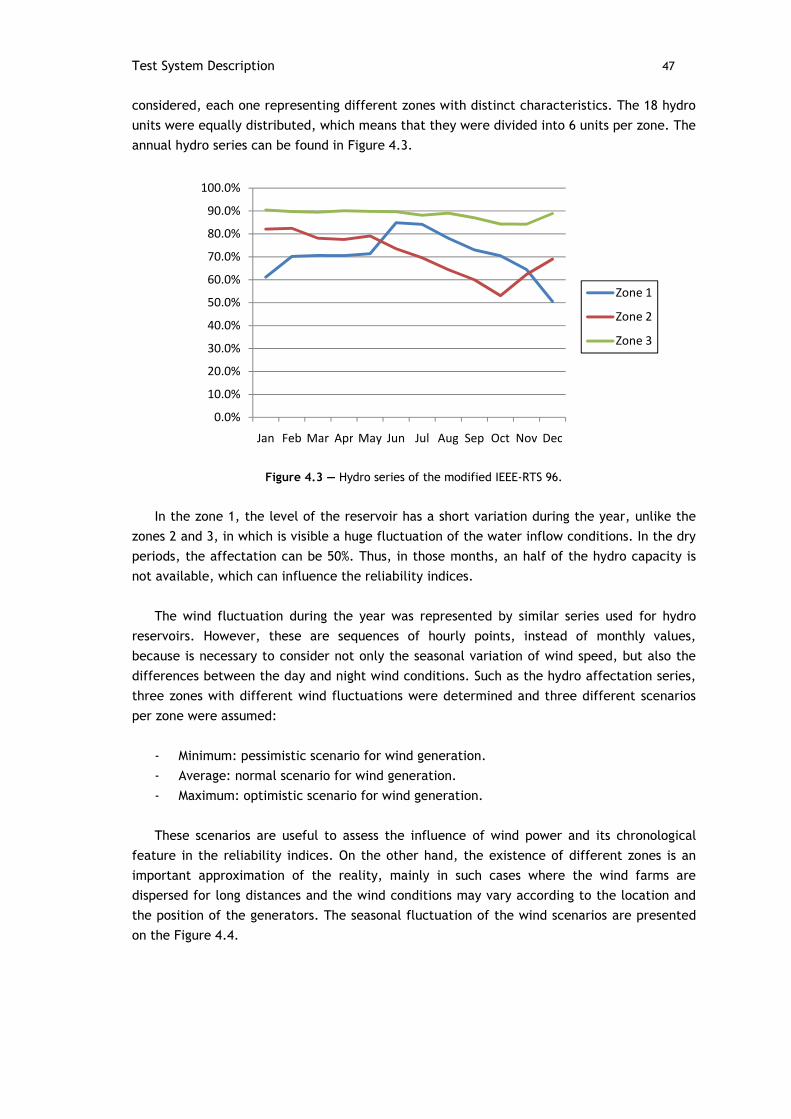
Test System Description 47
considered, each one representing different zones with distinct characteristics. The 18 hydro
units were equally distributed, which means that they were divided into 6 units per zone. The
annual hydro series can be found in Figure 4.3.
Figure 4.3 — Hydro series of the modified IEEE-RTS 96.
In the zone 1, the level of the reservoir has a short variation during the year, unlike the
zones 2 and 3, in which is visible a huge fluctuation of the water inflow conditions. In the dry
periods, the affectation can be 50%. Thus, in those months, an half of the hydro capacity is
not available, which can influence the reliability indices.
The wind fluctuation during the year was represented by similar series used for hydro
reservoirs. However, these are sequences of hourly points, instead of monthly values,
because is necessary to consider not only the seasonal variation of wind speed, but also the
differences between the day and night wind conditions. Such as the hydro affectation series,
three zones with different wind fluctuations were determined and three different scenarios
per zone were assumed:
- Minimum: pessimistic scenario for wind generation.
- Average: normal scenario for wind generation.
- Maximum: optimistic scenario for wind generation.
These scenarios are useful to assess the influence of wind power and its chronological
feature in the reliability indices. On the other hand, the existence of different zones is an
important approximation of the reality, mainly in such cases where the wind farms are
dispersed for long distances and the wind conditions may vary according to the location and
the position of the generators. The seasonal fluctuation of the wind scenarios are presented
on the Figure 4.4.
0.0%
10.0%
20.0%
30.0%
40.0%
50.0%
60.0%
70.0%
80.0%
90.0%
100.0%
Jan Feb Mar Apr May Jun Jul Aug Sep Oct Nov Dec
Zone 1
Zone 2
Zone 3

48 Application Results
MW
Figure 4.4 — Wind scenarios of the modified IEEE-RTS 96.
The sequence of the 8760 load points considered for the demand modeling can be found
in the reference [38]. The mean daily and monthly load is presented in Figure 4.5.
Figure 4.5 — Daily load of the modified IEEE-RTS 96.
The monthly load is shown on the Figure 4.6.
0.0%
10.0%
20.0%
30.0%
40.0%
50.0%
60.0%
70.0%
80.0%
Jan Feb Mar Apr May Jun Jul Aug Sep Oct Nov Dec
Avarage
Maximum
Minimum
0
1000
2000
3000
4000
5000
6000
7000
1 3 5 7 9 11 13 15 17 19 21 23
Daily Load
h

Test System Description 49
Figure 4.6 — Load seasonal variation in modified IEEE-RTS 96.
4.1.2 - Portuguese System 2015
The proposed methodology for reliability assessment was applied to the Portuguese
generation system expected for the year 2015. The data is available on the reference [40],
which consists of the planning configuration to the 2015 of Portuguese system. Although the
IEEE-RTS 96 is a universal system with a large amount of different characteristics, the
proposed methodology also should be done for realistic countries cases, which have their
peculiar load diagrams and normally a huge number of generators and distinct power sources.
As a matter of fact, Portuguese System to the 2015 configuration will has a significant
installed capacity coming from unconventional power sources, like Wind, Photovoltaic,
Biomass, Solar Thermal and Cogeneration. Moreover, the hydro penetration is high, not only
by the existence of big hydro plants, but also because of the increasing number of mini-hydro
units. The next chart shows the percentage of each power source in the 19935 MW of
installed capacity:
Figure 4.7 — Energy Sources of Portuguese system.
As shown in Figure 4.7, hydro and wind installed capacities represent approximately 50%
of the Portuguese generation. However, these capacities are not always available, due to
0
1000
2000
3000
4000
5000
6000
7000
Jan Feb Mar Apr May Jun Jul Aug Sep Oct Nov Dec
Monthly load
34%
26%3%
25%
5%
7%Thermal
Hydro
Mini-Hydro
Wind
Cogeneration
Other unconventional
sources
MW

50 Application Results
their time dependence. Thus, the hydro and wind fluctuation should be described by
sequences of values, such as those used for IEEE-RTS 96.
The hydro generation was divided into 38 reservoirs with different levels and seasonal
fluctuations. In Figure 4.8 below, four examples of hydro series are presented to illustrate
the variation of the reservoirs during the year.
Figure 4.8 — Examples of reservoirs’ levels variation.
These hydro sequences are an average of historical values, unlike those used in IEEE-RTS
96 case. In fact, 15 years of levels observation (since 1990 to 2005) were considered to obtain
these series. Although some seasonal variation can be found, mainly in Reservoir 1, the
monthly hydro fluctuation is not deep, probably due to the huge capacity of these reservoirs.
Thus, if lower capacity units are observed, a higher variation is expected, for example in
mini-hydro systems.
Figure 4.9 — Mini-Hydro sequence of the Portuguese systems.
0.0%
20.0%
40.0%
60.0%
80.0%
100.0%
120.0%
Jan Feb Mar Apr May Jun Jul Aug Sep Oct Nov Dec
Res A
Res B
Res C
Res D
0.0%
5.0%
10.0%
15.0%
20.0%
25.0%
30.0%
35.0%
40.0%
45.0%
50.0%
Jan Feb Mar Apr May Jun Jul Aug Sep Oct Nov Dec
Mini-Hydro

Test System Description 51
As shown in Figure 4.9 above, which represent an average of 15 years of mini-hydro
capacities affectation, distinct periods can be found. As expected, during the dry months
(July to September) the capacity can decrease to 5% and during wet periods (November to
March) the hydro availability may increase up to 50%.
Such as the IEEE-RTS 96, the wind representation is done by a sequence of 8760 points,
which allows an hourly evaluation of the wind speed. On the other hand, the wind fluctuation
has also seasonal characteristics that affect the power output of the wind farms during the
year.
In the Portuguese system, three historical series based on historical years were chosen
and seven regions with different wind fluctuations were considered. Figure 4.10, Figure 4.11
and Figure 4.12 illustrate the seasonal dependence of wind power affectation through the
region monthly curves for the years above.
Figure 4.10 — Wind fluctuation of the year 1.
Figure 4.11 — Wind fluctuation of the year 2.
0.0%
10.0%
20.0%
30.0%
40.0%
50.0%
60.0%
70.0%
80.0%
Jan Feb Mar Apr May Jun Jul Aug Sep Oct Nov Dec
Zone 1
Zone 2
Zone 3
Zone 4
Zone 5
Zone 6
Zone 7
0.0%
10.0%
20.0%
30.0%
40.0%
50.0%
60.0%
70.0%
Zone 1
Zone 2
Zone 3
Zone 4
Zone 5
Zone 6
Zone 7

52 Application Results
Figure 4.12 — Wind fluctuation of the year 3.
The Figure 4.13 contains the comparison of the affectation percentages that occur during
the three years. The curves below were obtained through the calculation of the average of
region series for each year.
Figure 4.13 — Comparison of the wind variation.
The seasonal characteristic of the years 1 and 2 are similar, in spite of the increasing
affectation at the end of year 3. It is curious to observe the lack of wind speed during the
beginning of year 3, which may have a negative influence on the reliability indices for these
months, if this series is considered.
As mentioned above, the load is represented through a sequence of hourly points. Its
seasonal characteristic is presented in Figure 4.14. As expected, the load has a small
variation during the year, because the consumer habits do not have deeply changes.
However, a higher energy demand during the winter months exists.
0.0%
10.0%
20.0%
30.0%
40.0%
50.0%
60.0%
Jan
Fe
b
Ma
r
Ap
r
Ma
y
Jun
Jul
Au
g
Se
p
Oct
No
v
De
c
Zone 1
Zone 2
Zone 3
Zone 4
Zone 5
Zone 6
Zone 7
0.0%
5.0%
10.0%
15.0%
20.0%
25.0%
30.0%
35.0%
40.0%
45.0%
50.0%
Jan Feb Mar Apr May Jun Jul Aug Sep Oct Nov Dec
Year 1
Year 2
Year 3

Test System Description 53
Figure 4.14 —Load seasonal variation of the Portuguese system.
The daily characteristic of the load, presented on the Figure 4.15., describe the typical
Portuguese consumption habits:
Figure 4.15 — Load daily variation of the Portuguese system.
4.2 - Electric Vehicles Load Modeling applied to IEEE-RTS 96
4.2.1 - Electric Vehicles penetration scenarios
In the Merge Project study [39], EVs scenarios for a group of six European Union countries
were determined. Thus, the daily load diagram for each country was obtained and the
penetration of EVs during the day was predicted. The magnitude of the load and its variation
were considered and the results of the dumb charging and smart charging scenarios were
presented. The expected load diagram for each country is shown on the following charts.
0
1000
2000
3000
4000
5000
6000
7000
8000
9000
10000
Jan Feb Mar Apr May Jun Jul Aug Sep Oct Nov Dec
Load
0
1000
2000
3000
4000
5000
6000
7000
1 3 5 7 9 11 13 15 17 19 21 23
Daily Load
MW
MW
h

54 Application Results
Country A
Dumb charging
Figure 4.16 — Country A: Dumb Charging.
The Figure 4.16 shows a typical load diagram of the Country A. The baseline represents
normal demand, which has a 65.022 MW peak load at 18:00, and the red curve represents the
typical electric vehicle penetration (10% of its total vehicle fleet). As one can see, the EVs
demand create a new peak at 20:00, which may increase energy not supply.
Smart Charging
Figure 4.17 — Country A: Smart Charging.
In the Smart Charging scenario for the Country A, presented in Figure 4.17, it is possible
to observe that the EVs demand was moved to the night period, because the baseline has
lower values. In fact, this shift can occur, because the cars are usually parked during the
night, which allows a free management of the load in that period.
0
10,000
20,000
30,000
40,000
50,000
60,000
70,000
80,000
0:0
0
1:4
5
3:3
0
5:1
5
7:0
0
8:4
5
10
:30
12
:15
14
:00
15
:45
17
:30
19
:15
21
:00
22
:45
EV charging load
Baseline demand
0
10,000
20,000
30,000
40,000
50,000
60,000
70,000
0:0
0
1:3
0
3:0
0
4:3
0
6:0
0
7:3
0
9:0
0
10
:30
12
:00
13
:30
15
:00
16
:30
18
:00
19
:30
21
:00
22
:30
EV charging load (smart)
Baseline demand
MW
MW

Electric Vehicles Load Modeling applied to RTS System 55
Country B
Dumb Charging
Figure 4.18 — Country B: Dumb Charging.
The baseline demand of the Country B, presented in Figure 4.18, shows a peak of 51.970
MW at 17:00. However, when people come home in the evening period and plug their cars
into the grid, the peak is moved to one hour later and its magnitude is 56.404 MW.
Smart Charging
Figure 4.19 — Country B: Smart Charging.
As one can see in Figure 4.19, after 22:00 the baseline demand decreases and starts
increasing at 6:30 in the morning. Thus, the smart control moved charging to that period and
the EVs demand is now distributed during the night.
0
10,000
20,000
30,000
40,000
50,000
60,000
0:0
0
1:3
0
3:0
0
4:3
0
6:0
0
7:3
0
9:0
0
10
:30
12
:00
13
:30
15
:00
16
:30
18
:00
19
:30
21
:00
22
:30
EV charging load
Baseline demand
0
10,000
20,000
30,000
40,000
50,000
60,000
0:0
0
1:3
0
3:0
0
4:3
0
6:0
0
7:3
0
9:0
0
10
:30
12
:00
13
:30
15
:00
16
:30
18
:00
19
:30
21
:00
22
:30
EV charging load (smart)
Baseline demand
MW
MW
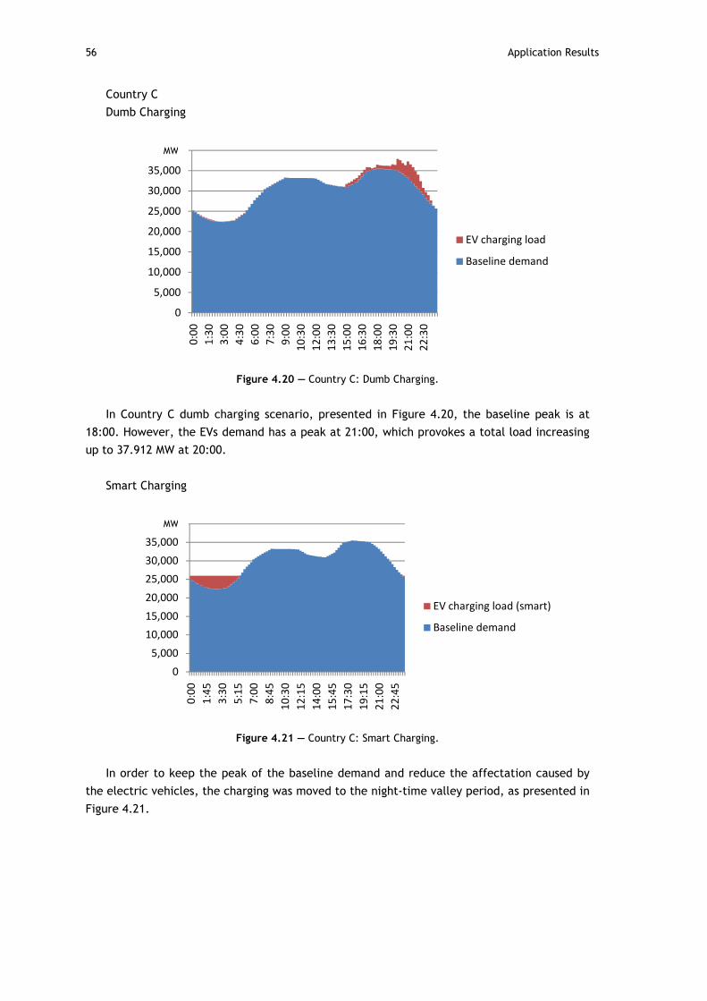
56 Application Results
Country C
Dumb Charging
Figure 4.20 — Country C: Dumb Charging.
In Country C dumb charging scenario, presented in Figure 4.20, the baseline peak is at
18:00. However, the EVs demand has a peak at 21:00, which provokes a total load increasing
up to 37.912 MW at 20:00.
Smart Charging
Figure 4.21 — Country C: Smart Charging.
In order to keep the peak of the baseline demand and reduce the affectation caused by
the electric vehicles, the charging was moved to the night-time valley period, as presented in
Figure 4.21.
0
5,000
10,000
15,000
20,000
25,000
30,000
35,000
40,000
0:0
0
1:3
0
3:0
0
4:3
0
6:0
0
7:3
0
9:0
0
10
:30
12
:00
13
:30
15
:00
16
:30
18
:00
19
:30
21
:00
22
:30
EV charging load
Baseline demand
0
5,000
10,000
15,000
20,000
25,000
30,000
35,000
40,000
0:0
0
1:4
5
3:3
0
5:1
5
7:0
0
8:4
5
10
:30
12
:15
14
:00
15
:45
17
:30
19
:15
21
:00
22
:45
EV charging load (smart)
Baseline demand
MW
MW

Electric Vehicles Load Modeling applied to RTS System 57
Country D
Dumb Charging
Figure 4.22 — Country D: Dumb Charging.
As one can see in Figure 4.22, Country D is a small country with a baseline load peak is
7339 MW. The peak of EVs penetration occurs at 20:00 increasing the total load up to 7.902
MW at this time.
Smart Charging
Figure 4.23 — Country D: Smart Charging.
Such as the previous countries, the electric vehicles charging is moved to the night period
and does not affect the total demand peak, as presented in Figure 4.23.
0
1,000
2,000
3,000
4,000
5,000
6,000
7,000
8,000
9,000
0:0
0
1:3
0
3:0
0
4:3
0
6:0
0
7:3
0
9:0
0
10
:30
12
:00
13
:30
15
:00
16
:30
18
:00
19
:30
21
:00
22
:30
EV charging load
Baseline demand
0
1,000
2,000
3,000
4,000
5,000
6,000
7,000
8,000
0:0
0
1:3
0
3:0
0
4:3
0
6:0
0
7:3
0
9:0
0
10
:30
12
:00
13
:30
15
:00
16
:30
18
:00
19
:30
21
:00
22
:30
EV charging load (smart)
Baseline demand
MW
MW

58 Application Results
Country E
Dumb Charging
Figure 4.24 — Country E: Dumb Charging.
The Country E, see Figure 4.24, presents some differences in its baseline diagram. In fact,
the night-time valley starts later and it is even deeper than in the other countries. The peaks
of the baseline demand and the EVs penetration occur almost simultaneously, which leads to
a load increasing up to 8.561 MW at 20:00.
Smart Charging
Figure 4.25 — Country E: Smart Charging.
The electric vehicles demand was distributed between the hours of the night-period
valley in Figure 4.25. It is important to stress that this valley happens later than the other
countries, between 1:00 and 7:30.
0
1,000
2,000
3,000
4,000
5,000
6,000
7,000
8,000
9,000
0:0
0
1:4
5
3:3
0
5:1
5
7:0
0
8:4
5
10
:30
12
:15
14
:00
15
:45
17
:30
19
:15
21
:00
22
:45
EV charging load
Baseline demand
0
1,000
2,000
3,000
4,000
5,000
6,000
7,000
8,000
9,000
0:0
0
1:4
5
3:3
0
5:1
5
7:0
0
8:4
5
10
:30
12
:15
14
:00
15
:45
17
:30
19
:15
21
:00
22
:45
EV charging load (smart)
Baseline demand
MW
MW

Electric Vehicles Load Modeling applied to RTS System 59
Country F
Dumb Charging
Figure 4.26 — Country F: Dumb Charging.
The Country F, see Figure 4.26, is the smallest system with a baseline peak of 4.454 MW
at 17:45. The EVs penetration moves this peak to 18:00 and increases it up to 4.720 MW.
Smart Charging
Figure 4.27 — Country F: Smart Charging.
The smart control move charging to the night period and the peak of EVs demand occurs
now at 5:00, as presented in Figure 4.27.
0
500
1,000
1,500
2,000
2,500
3,000
3,500
4,000
4,500
5,000
0:0
0
1:3
0
3:0
0
4:3
0
6:0
0
7:3
0
9:0
0
10
:30
12
:00
13
:30
15
:00
16
:30
18
:00
19
:30
21
:00
22
:30
EV charging load
Baseline demand
0
500
1,000
1,500
2,000
2,500
3,000
3,500
4,000
4,500
5,000
0:0
0
1:4
5
3:3
0
5:1
5
7:0
0
8:4
5
10
:30
12
:15
14
:00
15
:45
17
:30
19
:15
21
:00
22
:45
EV charging load (smart)
Baseline demand
MW
MW

60 Application Results
4.2.2 - Load model applied to the system based on IEEE-RTS 96
The information about generation system and unconventional sources of the countries
previously presented is not available. Hence, in order to evaluate their electric vehicles
penetration, a system should be used. Thus, these daily EVs demands were converted into
annual sequences of 8760 points and joined to the system based on IEEE-RTS 96, which was
already presented. However, as the magnitudes of the EVs penetration are different for each
country, they were modified according to the IEEE-RTS 96 load. This step, described on the
following equation, is vital to do a coherent comparison between the countries.
%�� (IEEE − RTS 96) = %�� (�YZ����) × %��� �Y�� (IEEE − RTS 96)%��� �Y�� (�YZ���� �������) (4.2)
As a matter of fact, this adaptation aims to assess the reliability of the EVs demand
shapes applied to the system based on IEEE-RTS 96. In other words, the goal of this section is
not the evaluation of each country EVs penetration, which only would be possible if the
countries generation data were known.
As previously shown in the smart charging diagrams, the smart control moved the EVs
charging to lower load periods. Thus, the results of the EVs load models are dependent on the
baseline diagram of each country in this kind of scenarios. Therefore, these load models may
not be suitable adapted to the IEEE-RTS 96 load, since the control was not based on it.
However, the main aspects of the countries daily diagrams are kept in IEEE-RTS 96 load.
The methodology proposed in chapter 3 was applied to the system based on IEEE-RTS 96,
including the electric vehicles scenarios of the six European countries mentioned before. In
order to assess the reliability impact of those shapes in the system and to compare the
differences between the countries and the scenarios, LOLE, LOLF and EENS were obtained.
Moreover, the monthly indices were also calculated so that the annual fluctuation can be
evaluated.
The tests were done in a personal computer with an Intel Core i5 processor running at
2.27 GHz, with 4 GB of random access memory. The algorithms were implemented through
the Eclipse from Sun, in Java environment. The Operating system used was Microsoft
Windows7 - 64 bits.
The Figure 4.28 presents the annual LOLE of each country.

Electric Vehicles Load Modeling applied to RTS System 61
Figure 4.28 — LOLE assessment for each country, considering different scenarios.
In the dumb charging scenario, the loss of load expectation (LOLE) dramatically
increased. A and B were the most affected countries, because their charging periods are
highly concentrated between 18:00 and 20:00. As shown on the load diagram, the vehicles
demand points of the country C are spreading during the evening, which lead to a lower loss
of load expectation.
When a smart charging scenario is considered, the LOLE decreased significantly and the
penetration of electric vehicles does not affect the loss of energy. This fact suggests that the
demand baselines of the countries are similar to the IEEE-RTS 96 load during the night
periods, for which the electric charging was moved. Thus, although the smart control was not
done considering the IEEE-RTS 96 load, it is possible to conclude that these EVs penetration
scenarios fit on it. This idea is even stressed if the Country E is considered, because a small
difference between the Smart Charging and No EVs scenarios is found. As stated before, in
this country the night-time valley of the baseline diagram occurs later than the others, which
leads to a penetration of EVs in the first hours of the morning.
The Loss of load frequency increases for the dumb charging scenario, mainly in the
counties A and B. The next Figure 4.29 shows the annual LOLF assessment:
Figure 4.29 — LOLF assessment for each country, considering different scenarios.
0.00E+00
5.00E-01
1.00E+00
1.50E+00
2.00E+00
2.50E+00
3.00E+00
Dumb Charging
smart Charging
No Evs
0.00E+00
5.00E-01
1.00E+00
1.50E+00
2.00E+00
2.50E+00
Dumb Charging
smart Charging
No Evs
h/yr
occ/yr

62 Application Results
The energy not supply calculation for each country is illustrated in Figure 4.30. The same
characteristic is visible in the countries A and B for the dumb charging scenario. On the other
hand, the country C presents a low energy not supplied, since the spreading electric vehicles
penetration previously mentioned.
Figure 4.30 — EENS assessment for each country, considering different scenarios.
In the smart charging scenario, a higher value exists for the country E, which is provoked
by the shift on the night-period valley. However, in comparison with the dumb charging
scenario, this value is not significant.
4.3 - Portuguese System case
In this section the proposed methodology will be used to assess the security of supply of
the Portuguese generation system, considering a penetration of EVs. The Portuguese curve
from Merge Project results, already presented, was chosen to represent the daily EVs
demand. The wind sequence for the year 3 was used.
The tests were done in a personal computer with an Intel Core i5 processor running at
2.27 GHz, with 4 GB of random access memory. The algorithms were implemented through
the Eclipse from Sun, in Java environment. The Operating system used was Microsoft
Windows7 - 64 bits.
The mean time to compute the Portuguese System indices was 10 minutes and 11
seconds.
The Figure 4.31 below shows the comparison of the LOLE assessment considering the two
distinct management approaches scenarios: dumb charging and smart charging.
0.00
100.00
200.00
300.00
400.00
500.00
600.00
700.00
Dumb Charging
smart Charging
No Evs
MWh

Portuguese System case 63
Figure 4.31 — LOLE assessment for Portuguese system, considering 3 different EVs penetrations.
In the dumb charging scenario is expected that the system cannot supply the total
demand in 77 hours, as presented in Figure 4.31. Similarly to the test done in the system
based on IEEE-RTS 96, this scenario dramatically affects the Portuguese security of supply. On
the other hand, the smart charging completely solves this problem. In fact the difference
between this scenario and the baseline consideration is about 2.0x10⁻⁵ hours, which is
represents an insignificant period. This residual difference occurs, due to the ideal transfer
of the EVs penetration for the night periods. As shown on the Portuguese daily load diagram
this nocturne valley occurs and it is deep enough to receive this power without affect the
reliability indices.
The monthly LOLE was computed, so that the annual variation of the security of supply
can be evaluated and the both electric vehicles scenarios can be compared. The resultant
curve is illustrated on the Figure 4.32 below:
Figure 4.32 — Monthly Comparison of both management approaches.
0.00
10.00
20.00
30.00
40.00
50.00
60.00
70.00
80.00
90.00
Dumb Charging Smart Charging No Evs
LOLE assessment
0.00
5.00
10.00
15.00
20.00
25.00
30.00
35.00
40.00
jan feb mar apr may jun jul aug sep oct nov dec
Dumb Charging Smart Charging
h/ yr
h/ month

64 Application Results
In Figure 4.32 above is possible to observe that the difference between the management
approaches occurs, due the high LOLE value during the winter months, considering the dumb
charging scenario. As a matter of fact, in January their magnitude is 7 times more than the
smart charging. However, any seasonal variation was not included in the EVs penetration.
Hence, this difference is caused by the unconventional sources and the load fluctuation.
Thus, the constant increasing, provoked by the EVs, led to distinct results in monthly
assessment, which suggest that the reserve in winter months was not enough to bear the
dumb charging penetration.
The Figure 4.33 shows the Portuguese LOLF assessment for the same scenarios used in the
LOLE evaluation.
Figure 4.33 — LOLF assessment for Portuguese System, considering 3 different EVs penetrations.
The figure shows the high influence of the dumb charging in the reliability indices and an
ideal scenario of EVs penetration when the smart charging is considered. In fact the
frequency of the failures is also related with the probabilities. Hence, this result was
expected, despite of the enormous difference between the scenarios.
A well-being analyse was done to assess the security of supply when a failure of the
highest capacity unit occurs. Hence, a generator with 670 MW was removed from the system
as a deterministic criterion. The probabilities of the success states for each scenario were
calculated and they are shown on the next Figure 4.34:
0.00
5.00
10.00
15.00
20.00
25.00
30.00
35.00
40.00
Dumb Charging Smart Charging No Evs
LOLF assessment
occ/yr

Portuguese System case 65
Figure 4.34 — Success states probabilities of the well-being analysis for the different EVs penetrations.
The Table 4.1 shows the number of hours per year in each state, for the different
scenarios.
Table 4.1 — Number of hours per year in each state
No EVs Dumb Charging Smart Charging
Success states 8722.07 h 8572.14 h 8722.07 h
Marginal States 32.35 h 110.21 h 32.36 h
Loss of Load states 5.5624 h 77.6333 h 5.5624 h
As illustrated on the Figure 4.34, even when the highest capacity is removed from the
generation system, the security of supply for the smart charging scenario is not affected.
Considering this fact, is possible to conclude that the Portuguese system can include EVs
without compromise their security of supply, if a smart charging penetration is used.
However, is important to remember that this scenario is not realistic, since it unrealistically
transfers the charging power for the convenient times.
0.84
0.86
0.88
0.9
0.92
0.94
0.96
0.98
1
jan feb mar apr may jun jul aug sep oct nov dec
No Evs
Dumb Charging
Smart Charging

66 Application Results

Chapter 5
Conclusions and Future Work
5.1 - Conclusions
This thesis assessed the impact of the electric vehicles penetration on the security of
supply point of view, through the development and implementation of an analytical
methodology considering time dependent characteristics of power system. The information
used was based on the Merge project, which aims to evaluate methods to model and optimize
electric systems that contain EVs and develop a management concept to integrate these
vehicles in the electric system. At the end of this evaluation, some topics should be stressed:
• Both management approaches tested are extreme scenarios. Dumb charging
dramatically affects the generation systems (security of supply), since it adds the
EVs penetration to the daily load peaks. On the other hand, the smart charging is
an ideal scenario that fills the night-time load valley and does not influence the
reliability indices. Hence, more approach should be proposed so that the results
become more realistic.
• In the Portuguese system case, the influence of dumb charging scenario on the
security of supply is significant, mainly in the winter months. During the year
assessed, the unconventional source capacities were not high enough in
comparison with load and the EVs penetration.
• The proposed methodology cans suitable represent the chronology of the
unconventional sources and the electric vehicles. Hence, this approach is an
interesting alternative to the Sequential Monte Carlo simulation, since its running
time is considerable lower without lose the accuracy of the results. Obviously,
the SMCS is a flexible way to represent non Markovian models and other
representations, which is a very hard task on analytical approaches. However,
more research is necessary on this area in order to achieve more realistic
representation.

68 Conclusions and Future Work
• In fact, this methodology is useful to study the reliability impact of the EVs
penetration through the use of scenarios, and it has shown to be an efficient tool
to simulate the future management concepts to deal with the EVs integration in
electric grids.
• Time dependent characteristics are presented in the modern power system
paradigm, and its representation becomes imperative to reliability studies.
5.2 - Future Work
One of the most important tasks in any research work is to identify topics that must be
addressed in the near future. Therefore, three major challenges could be cited as follows:
• An interesting improvement in the proposed methodology could be the extension
of the assessment to the transmission system. In fact, the security of supply
considering EVs penetration strongly depends on the nodes where the vehicles are
connected. Hence, the evaluation of the failures in the transmission lines would
beneficiate the reliability assessment of the system.
• In the EVs field, more realistic scenarios within the two extremes approaches
(smart charging and dumb charging) must be presented. Furthermore, the
concept of vehicle to grid, in which the EV can deliver the energy back to the
grid, scenario should be assessed.
• To identify distributional aspects of the reliability indices presented are an
interesting challenge through the analytical ways. Today, only SMCS make
possible to assess this characteristics of the indices.

References
[1] Fleet, Bernard and K. Li, James., ‘Situation Analysis for the Current State of Electric
Vehicle Technology’, Electric Vehicle Technology Roadmap Visioning Meeting, 2008.
[2] International Energy Agency., ‘Technology Road Map Electric and plug-in hybrid electric
vehicles (EV/PHEV)’, 2009.
[3] Peças Lopes, J.A, Soares, F.J., Rocha Almeida, P.M., ‘Indentifying Management
Procedures to Deal with Connection of Electric Vehicles in the Grid’, IEEE PowerTech
Bucharest, 2009.
[4] Peças Lopes, J.A., Moreira, C.L.,Madureira., A.G., ‘Defining Control Strategies for
MicroGrids Islanded Operation’ , IEEE Transactions on Power Systems, vol.21, June 2006, pp
916-924.
[5] Gil, N.J, Peças Lopes, J.A., ‘Hierarchical Frequency Control Scheme for Islanded Multi-
MicroGrids Operation’, Proceedings of IEEE Lausanne Power Tech2007, Switzerland, July
2007.
[6] Peças Lopes, Rocha Almeida, P.M, J.A, Soares, F.J., C.L.,Moreira., ‘Electric Vehicles in
Isolated Power Systems: Conceptual Framework and Contributions to Improve the Grid
Resilience’, Conference on Control Methodologies and Technology for Energy Efficiency, Vila
Moura Portugal, March 2010.
[7] Department for Business Enterprise & Regulatory Reform: Department for Transport,
‘Investigation into Scope for the Transport Sector to Switch to Electric Vehicles and Plug-in
Hybrid Vehicles’, United Kingdom, October 2008.

70 References
[8] Mayor of London, ‘London´s Electric Vehicle Infrastructure Strategy’, December 2009.
[9] Billinton, Roy and Allan, Ronald N., ‘Power system reliability in perspective’, IEE J.
Electronics Power, vol. 30, 1984, pp. 231-236.
[10] Rosa MA. ‘Multi-Agent Systems Applied to Assessment of Power Systems’. Ph.D. Thesis
approved by the Faculty of Engineering of University of Porto. February 2010.
[11] Leite da Silva AM, Cassula R, Billinton R, Manso LAF. ‘Integrated Reliability Evaluation of
Generation, Transmission and Distribution Systems’. IEE Proc. Gener. Transm. Distrib., 2002;
149(1): 1-6.
[12] Billinton, Roy and Allan, Ronald N., ‘Reliability Evaluation of Power Systems’, Second
Edition, New York, Plenum Press, 1996.
[13] Brown RE. ‘Electric Power Distribution Reliability’. New York: Marcel Dekker, Inc., 2002.
[14] Billinton R, Allan RN. ‘Reliability Evaluation of Engineering Systems: Concepts and
Techniques’. New York: Plenum Press, 1992.
[15] Allan, R.N., Leite da Silva, A.M., Abu-Nasser,A.A., Burchett, R.C., ‘Discrete Convolution
in Power System Reliability’, IEEE Transactions on Power Systems, vol.R-30, No 5, December
1981, pp 452-456.
[16] Leite da Silva, A.M., Melo, A.C.G., Cunha, S.H.F., ‘Frequency and duration method for
reliability evaluation of large-scale hydrothermal generating systems’, IEE Proceedings-
Generation, Transmission and Distribution, vol. 138, 1991, pp. 94-102.
[17] Rau, N.S. and Schenk, K.F., ‘Applications Fourier Methods for Evaluation of Capacity
Outage Probabilities’, IEEE Winter Power Meeting 1979, Paper No. A-79-103-3.
[18] Leite, A.P. and Borges, C.L.T, ‘Probability wind farms generation model for reliability
studies applied to Brazilian sites’, IEEE Transactions on Power Systems, vol. 21, No. 4,
November 2006, pp 1493-1501.
[19] Liu, X, Chowdhury, A.A. and Koval, D.O., ‘Reliability evaluation of a wind-diesel-battery
hybrid power system’, Industrial and Commercial Power System Technical Conference, ICPS
2008. IEEE/IAS; 2008, pp 1-8.
[20] Singh, C and Lago-Gonzalez, A., ‘Reliability modeling of generations systems including
unconventional energy sources’, IEEE Transactions on Power Apparatus and Systems, vol.
PAS-104, No. 5, May 1985, pp 1049-1055.

71
[21] Singh, C and Kim, Y., ‘An efficient technique for Reliability analysis of power systems
including time dependent sources’, IEEE Transactions on Power Systems, vol.3, No. 3, August
1988, pp. 1090-1096.
[22] Pereira MVF, Balu NJ. ‘Composite Generation/Transmission Reliability Evaluation’. Proc.
of the IEEE, 1992; 80(4): 470-491.
[23] Manso LAF, Leite da Silva AM. ‘Non-Sequential Monte Carlo Simulation for Composite
Reliability Assessment with Time Varying Loads’. Magazine Controle & Automação, 2004;
15(1): 93-100, (in Portuguese).
[24] V. Miranda, L. Carvalho, M. Rosa, A.M. Leite da Silva, C. Singh. ‘Improving Power System
Reliability Calculation Efficiency with EPSO Variants’. IEEE Trans. on Power Systems, 2009,
24(4), 1772-1779.
[25] Leite da Silva AM, Schmitt WF, Cassula AM, Sacramento CE. ‘Analytical and Monte Carlo
Approaches to Evaluate Probability Distributions of Interruption Duration’. IEEE Trans. on
Power Systems, 2005; 20(3): 1341-1348.
[26] Billinton R, Wangdee W. ‘Delivery Point Reliability Indices of a Bulk Electric System
Using Sequential Monte Carlo Simulation’. IEEE Trans. on Power Delivery, 2006; 21(1): 345-
352.
[27] Rubinstein RY. ‘Simulation and Monte Carlo Method’. New York: John Wiley & Sons;
1980.
[28] Rubinstein RY, Kroese DP. ‘Simulation and Monte Carlo Method - 2nd Edition’. New York:
John Wiley & Sons, 2008.
[29] Billinton R, Li W. ‘Reliability Assessment of Electric Power System Using Monte Carlo
Methods’. New York: Plenum Press, 1994.
[30] Mello JCO, Pereira MVF, Leite da Silva AM. ‘Evaluation of Reliability Worth in Composite
Systems Based on Pseudo-Sequential Monte Carlo Simulation’. IEEE Trans. on Power Systems,
1994; 9(3): 1318-1326.
[31] Leite da Silva AM, Manso LAF, Mello JCO, Billinton R. ‘Pseudo-Chronological Simulation
for Composite Reliability Analysis with Time Varying Loads’. IEEE Trans. on Power Systems,
2000; 15(1): 73-80.
[32] Gomes, F.M.B., Oliveira, G.C., Pereira, M.V.F., ’Reliability evaluation in hydrothermal
generating Systems’, IEEE Transactions Apparatus and Systems, vol PAS-101, No.12, 1982.
[33] António Francisco Monteiro Dias Redondo, ‘Analytical Chronologic method to assess the
adequacy of the generation system.’, MSc Thesis approved by the Faculty of Engineering of
University of Porto, February 2010. (in Portuguese).

72 References
[34] Stremel, John P., ‘Sensitivity study of the cumulant method of calculating generation
system reliability’, IEEE Transactions on Power Systems, vol. PAS-100, No. 2, Feb.1981, pp
771-778.
[35] IEEE APM Subcommittee. ‘IEEE Reliability Test System’. IEEE Trans. on PAS, 1979; 99(6):
2047-2054.
[36] Ringlee, Robert Jn and Wood, Allen J., ‘Frequency and Duration Methods for Power
System Reliability Calculations: II-Demand Model and Capacity Reserve Model’, IEEE
Transactions on Power Systems, vol. PAS-88, No. 4, April 1969, pp 375-388.
[37] Singh, C. and Chen, Q., ‘Equivalent load method for calculating frequency & duration
indices in generation capacity reliability evaluation’, IEEE Transactions on Power Systems,
vol. PWRS-1, No. 1, February 1986, pp 101-107.
[38] The IEEE Reliability Test System 1996. ‘A Report Prepared by the Reliability Task Force
of the Application of Probability Methods Subcommittee - IEEE Reliability Test System’. IEEE
Trans. on Power Systems, 1999; 14(3): 1-8.
[39] MERGE Team, ‘Mobile Energy Resources in Grids of Electricity - Identification of Traffic
Patterns and Human Behaviors’, WP 1, Task 1.5, D 1.1, April 2010.
[40] REN, Technical Data ‘Provisional Values 2009’, Rede Eléctrica Nacional REN) S.A,
Fevereiro de 2009. Available on line: www.ren.pt.

73
Annex A - Test systems used to compare analytical methods
System: IEEE - RTS 79
Maximum Capacity in service: 3405 MW
Load: Single point load - 2850 MW
Table A.1 — RTS – 79 Generation System [35]
Number Capacity
(MW) FOR
5 12 0.02
4 20 0.1
6 50 0.01
4 76 0.02
3 100 0.04
4 155 0.04
3 197 0.05
1 350 0.08
2 400 0.12

74 Annex A – Test systems used to compare analytical methods
System: 48G
Maximum Capacity in service: 23070 MW
Load: 18000 MW.
Table A.2 — 48 Generators System [17]
Number Capacity (MW) FOR
1 685 0.15
1 685 0.16
1 685 0.18
1 644 0.21
1 600 0.12
4 547 0.08
8 531 0.1
4 525 0.06
4 514 0.12
1 400 0.065
8 287 0.13
1 206 0.2
1 200 0.0885
4 200 0.09
4 100 0.08
4 64 0.06

75
System: 116G
Maximum Capacity in service: 7952 MW
Load: Linear - two load points. Maximum: 6525 MW; Minimum: 2610
Table A.3 — 116 Generators System [15]
Number Capacity
(MW) FOR
3 11 0.0118
4 17.5 0.013
6 20 0.0134
9 28 0.0148
41 32 0.0154
4 40 0.0168
14 52 0.0188
2 55 0.0194
15 63 0.0207
1 66 0.0212
2 120 0.0304
4 124 0.0311
4 145 0.0347
4 335 0.067
3 500 0.095


