Planning of Distribution System with High Penetration

International Journal of Current Engineering and Technology E-ISSN 2277 – 4106, P-ISSN 2347 – 5161 ©2018 INPRESSCO®, All Rights Reserved Available at http://inpressco.com/category/ijcet

Research Article

574| International Journal of Current Engineering and Technology, Vol.8, No.3 (May/June 2018)

Planning of Distribution System with High Penetration Level for Distributed Generation in Smart Grid Reza Tajik* Bandar-e-Abbas University of Applied Science and Technology, Iran

Received 15 March 2018, Accepted 18 May 2018, Available online 22 May 2018, Vol.8, No.3 (May/June 2018)

Abstract Nowadays, the utilization of renewable energy resources in distribution systems (DSs) has been rapidly increased. Since distribution generation (DG) use renewable resources (i.e., biomass, wind and solar) are emerging as proper solutions for electricity generation. Regarding the tremendous deployment of DG, common distribution networks are undergoing a transition to DSs, and the common planning methods have become traditional in the high penetration level. Indeed, in conformity with the voltage violation challenge of these resources, this problem must be dealt with too. So, due to the high penetration of DG resources and nonlinear nature of most industrial loads, the planning of DG installation has become an important issue in power systems. The goal of this paper is to determine the planning of DG in distribution systems through smart grid to minimize losses and control grid factors. In this regard, the present work intending to propose a suitable method for the planning of DSs, the key properties of DS planning problem are evaluated from the various aspects, such as the allocation of DGs, and planning, and high-level uncertainties. Also depending on these analyses, this universal literature review addressed the updated study associated with DS planning. In this work, an operational design has been prepared for a higher performance of the power distribution system in the presence of DG. Artificial neural network (ANN) has been used as a method for voltage monitoring and generation output optimization. The findings of the study show that the proposed method can be utilized as a technique to improve the process of the distribution system under various penetration levels and in the presence of DG. Also, the findings revealed that the optimal use of ANN method leads to more controllable and apparent DS. Keywords: distribution system, penetration level, distributed generation, smart grid Introduction

1 Today the broad improvement of distributed energy resources (DERs) and the liberalization of electricity market, traditional distribution networks are exposing a transition to active distribution systems (ADSs), and the traditional deterministic planning methods have become unsuitable under the high penetration of DERs. To date, power system analysis has been performed separately for transmission and distribution systems. Due to the small influence of distribution systems on transmission systems, separate analyses have had no accuracy problems in existing power systems. However, as the amount of distributed generation (DG) in distribution systems increases, neighboring distribution systems and even transmission systems can be affected by the distributed generation. Therefore, a power system operator needs a new system to analyze the power system, one that considers the mutual interactions between the transmission and distribution systems (Jaewan Suh, 2017). *Corresponding author’s ORCID ID: 0001-0002-0003-0004 DOI: https://doi.org/10.14741/ijcet/v.8.3.13

It is suggested that advanced power devices with converter and control system such as STATCOMs and SVCs can reduce reactive power problem, voltage instability, flicker and harmonic distortion and also improve power quality (Anil Gupta, 2014). The Energy demand is increasing because of a growing rate of urbanization, economic growth, increasing prosperity and enhancing per capita energy consumption. To fulfill the increasing energy demand need better cost effective and environment friendly solution. Renewable energy source based Distributed Power Generation is cost effective and environment friendly solution to fulfill the demand. Small scale Distributed Generation is connected to distribution systems. It is difficult to reach the good quality power with wind power generation because of vacillating behavior of wind speed that affects the voltage and active power output of electrical machine connected to wind turbine (Darshnaben K Metra, 2015). Benefits of Distributed Generation mentioned by Sandhu and Thakur (2014) as power generated and distributed near consumer end reduction in transmission loss, power reliability increases,

https://doi.org/10.14741/ijcet/v.8.3.13

Reza Tajik Planning of Distribution System with High Penetration Level for Distributed Generation in Smart Grid


reduction in greenhouse gas emissions compare to conventional power plants. So it is pointed out that in term of the vacillating nature of wind fluctuating power generates in the wind farm and it has negative impact on power quality and stability and voltage regulation in distribution system (Mamtha Sandhu, 2014). Qudaih and Mitani (2011) believed smart grid applications increases rapidly but still the clear definition of smart grid varies according to different grasps of the matter. Basically, the smart grids will be characterized by a two-way flow of electricity and information and will be capable of monitoring everything from power plants to customer preferences to individual appliance. In fact, finding the suitable scheme to approach a reliable distribution system to overcome all expected changes and applications due to the smart grid is a very crucial and wise task. An artificial intelligence technique has been introduced in form of artificial neural network (ANN) for voltage monitoring and generation output optimization. The results show an efficient utilization of neural network which results in more controllable and observable power distribution system. Wei Wang et al (2017) aiming to develop appropriate models and methodologies for the planning of ADSs, the key features of ADS planning problem are analyzed from the different perspectives, such as the allocation of DGs and ESS, coupling of operation and planning, and high-level uncertainties. The planning models and methods proposed in these research works are analyzed and categorized from different perspectives including objectives, decision variables, constraint conditions, and solving algorithms. The key theoretical issues and challenges of ADS planning are extracted and discussed. Meanwhile, emphasis is also given to the suitable suggestions to deal with these abovementioned issues based on the available literature and comparisons between them. Finally, several important research prospects are recommended for further research in ADS planning field, such as planning with multiple micro-grids (MGs), collaborative planning between ADSs and information communication system (ICS), and planning from different perspectives of multi-stakeholders [6]. Balamurugan et al (2012) modeled the IEEE 34 Node distribution test feeder using the commercial software package DIgSILENT power factory version 14. Solar photovoltaic generators are introduced as Distributed Generators (DGs) at various nodes and the impacts that DG produces on real and reactive power losses, voltage profile, phase imbalance and fault level of distribution system is studied. Simulated results obtained using load flow and short circuit studies are presented and discussed. Suh et al (2017) presents with applications and case studies a transmission and distribution integrated monitoring and analysis system for high DG penetration. The integrated system analyzes the

mutual interaction between the transmission and distribution systems due to DG. The preliminary evaluation of the DG connections is automated in this system, using real time online data. Case studies with practical data show the need and effectiveness of transmission and distribution integrated monitoring and analysis for real power systems with high DG penetration [8]. Fallahzadeh-Abarghouei et al (2013) proposes a new approach for distributed generations (DGs) planning by partitioning the original distribution systems into several separate zones. Then in operation stage a zonal voltage control method is presented which uses only local data and optimizes reactive power of the DGs where have been placed in previous stage. Both planning and operating problem are optimized using the well-known particle swarm optimization (PSO) algorithm. Finally, the proposed methods are evaluated on IEEE 123-bus unbalanced test system. The results demonstrate the ability and efficiency of the proposed methods. In this study an operational framework has been proposed with respect to ANN. The study aimed to investigate the power distribution system by monitoring the voltage profile with respect to load changes and choosing the optimum output of the distributed generation. So the aims of study are to obtain a smart grid by examine load and generation in a flexible manner and this study could be a base for further improvements in this regard. Distribution power system Distribution systems start from the distribution substation and deliver the power to the end users. Traditionally, the planning and operation of distribution systems have received less attention than transmission system which leads to the overdesign and inefficiency of distribution systems. Quick developing energy technology together with the environmental concerns has greatly increased the complexity of power grid and distribution systems, where the desire to increase the efficiency of energy distribution and consumption is increased (Rui Li, Desta Z. Fitiwi, 2017). The need to high quality and reliable power supply to consumers, smart grid has been identified as the next generation of electric power systems around the globe. In the context of smart grid, the modern distribution system is changing from passive to active by distributed generation, communication technology, and automation control devices (Zheng, Yu, 2015; Lund T, 2008). We can see the significantly increasing penetration of new power engineering technologies, such as renewable energy distributed generation (Anees, A.S, 2012) energy storage (Sweta, 2013) and other factors. There is a need to fully exploit the potential advantages of these new elements in smart distribution systems. The distribution system along with smart



devices, as the solution to the need for grid development, provides utilities with many benefits, including improved operational efficiency, flexibility and power quality (MihailAbrudean). However, despite those benefits, the planning of smart distribution system is a problem of vital importance since it concerns how the system is designed to achieve higher efficiency and reliability (Sardi, 2017). The planning methods of the existing distribution system are either inappropriate for practical use in dealing with the emerging elements or impossible to achieve the global optimal solution (Ahmadian, 2017). As a result, in-depth research is needed to solve these emerging and difficult problems in planning and operation (Liu W, 2017). Most of the existing researches focus on one type of elements in the distribution system without taking other components and their implications on the overall system performance into consideration (Karagiannopoulos, 2017). In addition, they seldom consider the effects of electricity market or quantify the economic value brought by the reliability of the updated distribution systems. Therefore, in order to improve the economic efficiency and sustainability of smart grids, this research develops advanced planning methods for better integration and operation of new emerging elements, especially the distributed generation and energy storage in modern distribution system. First, a novel method for optimal allocation of renewable distributed generator (DG) is proposed. The optimal allocation of DG can not only reduce power loss through the feeder, but also improve the voltage stability, which is beneficial to both the economy and security of distribution systems. Multi-objective function is applied to quantify the impact brought by the increasing penetration of renewable DGs (Humayd, 2017).

Distributed Generation

Distributed Generation (DG) is defined as small generation units of 30MW or less which are sited at or near customer sites to meet specific customer needs, to support economic operation of the distribution power system or both. In DG the energy generated and distributed by using small scale technology near to consumer end that’s why it is also termed as decentralized power generation. Distributed Generation technologies include Photovoltaic systems, Wind Turbines, Micro Turbines, Fuel Cell, Biomass, Small Hydroelectric generators, Energy storage and synchronous generator application supply active power to distributed system connected in proximity of the consumer. In the modern distribution systems, the loads may be supplied locally by DGs and some parts of distribution systems can be considered as zones which may be interconnected to each other’s and they can operate in grid connected or in islanded modes (Kumar Nunna, 2013).

Due to the emerging of renewable DGs in distribution grids, reverse power flow as well as intermittent fluctuations of active power lead to significant variations in voltage magnitudes of buses (F. Olivier, 2016). DG Planning The optimal planning of distribution system and zones design can be formulated effectively as an optimization problem. There are some different objectives in the proposed planning model to consider cost aspects. The cost objective function can be formulated as below:

,i ,i ,

1

( )N

c WT PV FC i

j

f C C C

where CWT, CPV, and CFC are total costs of wind turbine, photovoltaic and fuel cell respectively (F. Olivier, 2016; Mamtha Sandhu,, 2014). These costs could be calculated by Eq. (7):

, ,

PV, ,

FC, FC,

.

.

.

WT i WT WT WT i

i PV PV PV i

i FC FC i

C a b P

C a b P

C a b P

where ax and bx. Px , are fixed and variable components of DG installation cost. Impact of distributed generation on distribution power system As the configuration of power lines and protective relying in most existent power system assume a unidirectional power flow and are designed and operated on that presumption [9]. The integration of Distributed Generation presents new challenges for Distribution system planning and operations because of the above presumption. Previously the integration of DG was sufficiently small but nowadays integration of DG is growing. As far as utility concerned the high penetration level of DG in distribution systems may pose a threat to network in terms of Power Quality issues, voltage regulation, reliability and stability [24]. In recognition of the possible contrary impacts of DG on distribution systems and the requirement of uniform criteria and necessity for the interconnection of DG IEEE Standard 1547 have been created. IEEE 1547 first released in 2003 and incorporated into the Energy Policy Act of 2005. The Standard includes several provisions to reduced DG’s possible negative effects on power quality (MIT Study).

Artificial Neural Networks

The human brain has about 100 billion neurons, each of which has the possibility to connect with more than 10,000 other neurons. Data as electrical and chemical



signals have continuous flow in the brain. The human brain is responsible for processing incoming data from the five senses and is responsible for interpreting them and decided what operation should be carried out based on the data received. Remarkable abilities of the human brain, inspiring numerous studies that can simulate this complex structure and this has been done mainly by electrical circuits (Si L. Wang, 2016) . Artificial neural networks created based on biological networks; we have tried to simulate the behavior of biological neurons. These artificial networks could perform a part of the capabilities of the human brain. Multilayer perceptron neural networks and radial basis function and support vector machine are a variety of artificial neural networks and all of them has the same basic features, including nodes, layers and connections. Node is the smallest part of a network. Each node receives signals from connections, signals before applying the transfer function, are added together, and then the output signal released to other nodes to reach network output (Martin S, 2016). The input layer receives the data and performs the same independent variables as the dependent variable acts. Output depends on the number of dependent variable is the number of neurons. An artificial neural network connects multiple neurons. For example, feed forward and recurrent each can be monolayer or multilayer. One of the most common types of progressive networks, multi-layer perceptron (MLP) networks which has been used in this study, too. In a multi-layer perceptron network all input neurons in the input layer and the output of all neurons in the output layer and all hidden neurons are distributed in one or more hidden layers (Moreira, 2018). These networks consist of multi-layer networks. The first layer (input layer) fed into the grid system. Output layer of the network outputs are computed. Layer between the input layer and output layer are called hidden layers that data processing is done on them. Because the networks, which is said to be the progressive output of each layer is considered as input to the next layer (D’Addona, 2017).

Figure 1: structure of artificial neural networks

Since the function needs to be better able to model complex behavior covers various factors. For the most frequently used sigmoid function, because this function is a high potential in various research has shown. The function of the input data to values in the range between zero and one converted as follows:

In this function, a and b are parameters of the function. It seems that communication in terms of both behavior and theoretically may exist between different variables. It is clear that the neural network models to follow different test statistics are not. Rather, we seek to create conditions in which the neurons in the neural network to automatically be able to mimic the behavior of the variables. In other words, as far as possible and reasonable to require that the neural network model to provide the best conditions for a better achievement. Thus, in addition to using non-linear functions as activation function, it needs to combine variables in our ability to provide. To increase the hidden layer neural network is the best option. As a result, in addition to the output layer two hidden layers with a small number of neurons we consider. The figure below shows the structure of the neural network. In the below figure 8 inputs (eight independent variables) in the first layer (Hidden 1) with 10 neurons are entered, the output value of the function is the sigmoid activation function. Then the output, the input of the second hidden layer (Hidden 2). The output layer of the neural network model into layers to produce the final output and through an activation function, single output (dependent variable) is created.

70% of the records randomly selected for training the network and the algorithm of Levenberg-Marquardt (Samuel O. W., 2017). Training on MATLAB software tools we use. Consider the mean square error performance benchmarks for both the Test and Validation 30 percent of the records of accidents and the number of times (ie 15% for each) we choose. Below are the results of the implementation model.

In the above figure, it is clear that only a mere 19 reps neural network model has a fraction of a second to



reach the mean square error of 2.11 hundredths MSE = 0.0211, which is a good performance for this model. Another issue is that the trained neural network, to get the inputs (values of the independent variables) can be a independent variable (output) is defined as an estimate of the actual value of the dependent variable (Target). This is how to estimate the variability in the original variables to express something that can provide clear understanding of neural network models. Certainly such a relationship will be expressed as a linear regression, because the neural network model has worked to train with the lowest error rate of real output. In the area of training that about 70% of the general population is estimated to come closer to reality. The coefficient of determination for this function is equal to 0.77. Such a model for the test data and validation is also used. Although the coefficient of determination obtained by dramatically reduced but this model does not represent inefficiencies may be a sharp reduction in the number of records (from 70% to 15% of the total records) could have a significant impact. On the other hand, random sampling may provide better results in other performances. Another important point is that this model for all data (including training, testing or validation) used to do a fairly good coefficient of determination R2 = 0.56 is obtained. This result reflects the fact that the model has good performance in estimating the optimal output. At the end of this section, it can be concluded that ANN model could describe the behavior of the independent variables in a convenient feature to describe the values of the dependent variable. Proposed model In this study at the beginning we have to indicate the target system and perform the flow calculation to determine the voltage level at every node of the system. In this study a 33-bus distribution system is a

medium tension distribution and common system and remote areas which are the main target of smart grid applications, has been used. So, there are 33 input signals (N1-N33) for estimation purposes that represent the output of the DG unit for each node. On the other hand, there are 33 output signals for voltage profile estimation and only a single output signal for the total losses. So the power loss of system obtained and objective

function of minimum power loss calculated by the optimal output of the DG. At final train and build the

ANN RBF and ANN MLP that will be the tools used in further observations in the system. The suggested model will be fulfilled achieving smart grid, where

RBF-NN-C and MLP- NN-C is the block representing the RBF and MLP neural networks constructed by

Matlab after the training and validation process.

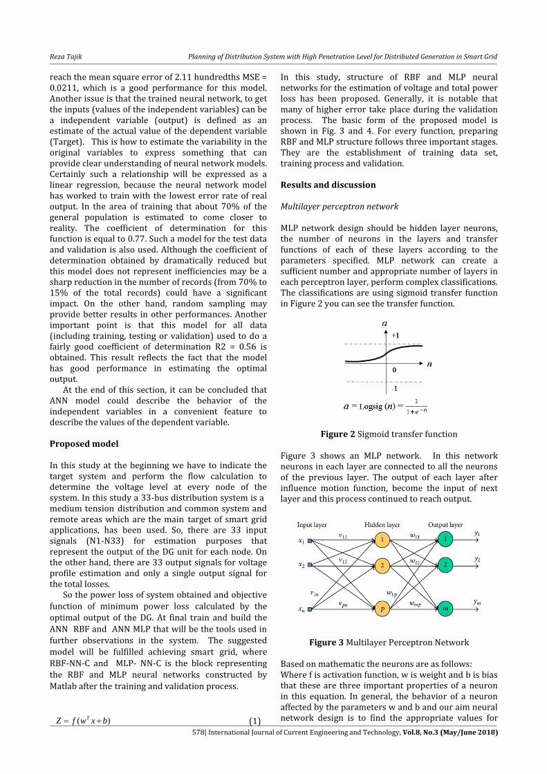
In this study, structure of RBF and MLP neural networks for the estimation of voltage and total power loss has been proposed. Generally, it is notable that many of higher error take place during the validation process. The basic form of the proposed model is shown in Fig. 3 and 4. For every function, preparing RBF and MLP structure follows three important stages. They are the establishment of training data set, training process and validation. Results and discussion Multilayer perceptron network MLP network design should be hidden layer neurons, the number of neurons in the layers and transfer functions of each of these layers according to the parameters specified. MLP network can create a sufficient number and appropriate number of layers in each perceptron layer, perform complex classifications. The classifications are using sigmoid transfer function in Figure 2 you can see the transfer function.

Figure 2 Sigmoid transfer function

Figure 3 shows an MLP network. In this network neurons in each layer are connected to all the neurons of the previous layer. The output of each layer after influence motion function, become the input of next layer and this process continued to reach output.

Figure 3 Multilayer Perceptron Network

Based on mathematic the neurons are as follows: Where f is activation function, w is weight and b is bias that these are three important properties of a neuron in this equation. In general, the behavior of a neuron affected by the parameters w and b and our aim neural network design is to find the appropriate values for (1) )( bxwfZ T



these parameters. MLP network learning method is based on back propagation learning algorithm. Evaluation of the MLP network To implement this network in the MATLAB environment, we first enter data (total number of data sample was 1532) and then divide them so that 70% of our input data so-called training data patterns are known our true and used during the training process, 15% of the validation data are unknown and is used during the training process and the remaining 15% of the data which are uncertain used after training. Levenberg-Marquardt function is used to train network that works better than the rest of the functions. According to previous statements by evaluating the performance of the three mean square error, root mean square error and correlation coefficient is measured.

n

i

ien

MSE1

2)(

1

(2)

MSEn

e

RMSE

n

i

i

1

2)(

(3)

Where ei is the difference between the experimental

data and the data were obtained by modeling.

Optimization of a model is minimizing the mean

squared error (MSE) and root mean square error and

also correlation coefficient tends to be one. We want to

teach a neural network, a maximum of a 3-layer

network that determines the number of neurons in the

first layer and the second in our possession. The

number of neurons should be selected so that the

neural network error reduces as much as possible.

Limit the number of neurons identified and adapted by Formula 4:

1

)()(2 1

oi

ooi

oinn

nnnknnn

(4)

Where n1 is number of neurons in the first layer, ni the

number of inputs, k samples and no number of our

outlets and the number of neurons that we choose for

this layer should not exceed this limit. Given that the

data in the study is 1532 sample, the allowable range

for the first layer neurons are neurons between 8 to

1226. The neural network training, a few of they can

improve network performance by changing these

factors include the number of layers, the number of

neurons and function will be transferred. To determine

the transfer function, initially for a certain number of

neurons (8 neurons), we compare the performance of

these functions. Comparison of the functions for

sample, see Table 1.

Table 1 Compares the performance of the MLP model by changing the transmission functions with 8 neurons

in the hidden layer

MSE R Transmission

functions

0.062294 0.31711 Compet

0.036595 0.68721 Hardlim

0.023072 0.81663 Hardlims

0.0000064518 0.99995 Logsig

0.0047039 0.96548 Netinv

0.0016117 0.9883 Poslin

0.022429 0.82272 Purelin

0.000027561 0.9998 Radbas

0.000009283 0.99993 Radbasn

0.00046514 0.99664 Satlin

0.00046473 0.99665 Satlins

0.000021368 0.99985 Softmax

0.000012896 0.99991 Tansig

0.00030082 0.99783 Tribas

As seen in the table 1 due to the correlation coefficient and the MSE, the Logsig function is the best way to teach a neural network considered in the study. Next step in network training is determining the number of layers and neurons in the hidden layer. The number of layers in the network that we have created includes three layers input layer, middle layer and output layer because more layers results more complex networks and are not appropriate. As can be seen in Table 1, forward network well responds to determine a layer in the middle layer, add the next layer is not much different and only network become more complex. In Table 2 By adding another layer to the desired network, we examine the network performance: Table 2 Compares the performance of the MLP model with second layer and change the number of neurons

in this layer

Network performance

The number of neurons in the second layer

The number of neurons in the

first layer

0.99994 1 8

0.99998 2 8

0.99997 3 8

0.99999 4 8

0.99999 5 8

0.99998 6 8

0.99999 7 8

0.99999 8 8

As discussed below, according to the MSE in Table 2, adding another layer of the network is not much difference in performance. Therefore, in this work, we will continue to teach network with three layers. In Table 3 by changing the number of neurons in the hidden layer, check the model performance and the results we report.



Table 3 Compares the performance of the MLP model by changing the number of neurons

RMSE MSE R The

number of neurons

0.00254 0.0000064518 0.99995 8 0.0010665 0.0000011374 0.99999 10 0.0014835 0.0000022009 0.99998 15

0.00198889 0.0000039556 0.99997 20 0.0022292 0.0000049695 0.99996 25 0.0022467 0.0000050447 0.99996 30 0.0024154 0.0000058342 0.99996 35 0.002429 0.0000059 0.99996 40

0.0046834 0.000021935 0.99984 50

Figure 4 Changes in MSE to change the number of neurons

As seen in Table 3 and Figure 4, the MLP will meet well and we change the number of neurons, we have not seen much change in the index. It can be concluded that for many samples that show changes slowly, this model would be appropriate. The mean square error, which indicates the efficiency of our target model, with 10 neurons in the hidden layer reaches its optimal value. The number of neurons increases the amount is less or more than the amount that is not good for us. Then, Figure 5 show matching laboratory outputs and target. Figure 6 shows the regression graph that represents values which are very close to a compliance test data and output neural network. Figure 7 shows a graph of error whose value fluctuated, but at one point reaches its maximum and Figure 8 shows the number of repetitions which indicates that the network is stopped in repetition 226.

Figure 5 matching laboratory outputs and target

Figure 6 Curve network performance

Figure 7 Error diagram

Figure 8 Stop repeating certain network

Radial Basis Function (RBF) network RBF network or neural networks based on radial basis

functions, is an approach to quantization information

and descriptive terms or otherwise reduce the size of

data using non-linear functions, the main data from

one space to another space that our nonlinear mapping

of the original space. This action we do because the

original space or input is not separated linearly, but

our space had this feature.

0

0.000005

0.00001

0.000015

0.00002

0.000025

8 10 15 20 25 30 35 40 50

MS

E

Neurons

MSE



Figure 9 ANN-RBF network structure

In fact, in this way we have multiple inputs and multiple kernels, or core that their numbers are not necessarily equal. So all the inputs and outputs of this kernel enter into a collector with a certain weight, and the output will be a scalar quantity. In this manner we enter with a mechanism from input to output space that is scalar. MLP model are really kernel role in the activation of functions that apply to collectors.

m

iii

T wxwy1

)( (4)

Where y is scalar output and the term after equality is sum weight of kernel functions and somehow, y is approximated core functions values; that is to say, in modeling by method of RBF, the input space by nonlinear mapping become the feature space and the linear order of this output will obtained and as if the kernel to be more, we estimate this process will be much easier, however, as the MLP we have limitations. RBF model is actually a type of MLP that collector has been used instead of the activation function. RBF function is a function that its value is related to input space from a central point, namely:

||)(||)()( 0xxfrfx (5)

m

iii xxwy

10 ||)(|| (6)

The output is the sum of weighted values of a function that is merely depends on the distance from its center. The dead ahead, xi are our data centers.

Evaluation of Radial Basis Function To implement this network in the MATLAB environment, there are several functions we have used two functions NEWRB and NEWRBE more than other. To estimate the function, NEWRB has more applications. What we expect from the network, such as network MLP, will be the mean square error close to zero as possible. Another factor in the RBF network, scattering name and by default it is considered, no

matter how much these factors increase the sphere of influence more and more RBF functions will overlap. Usually functions smoothly, by subtracting this amount, the number of neurons required will be more, therefore, for this type of functions we try to reduce this parameter unless we function with a lot of ups and downs. The maximum number of neurons that we can, with parameters determined MN and the number of our data, but we try to maximize the value to 0.1 to 0.2 considers the amount of data. We once had to create network in MLP and then pay for training but functions related to network RBF, coupled with a neural network training process is done incrementally. However, to enter data and apply the NEWRB, pay their modeling RBF method and 70% of our data and 30 percent training data to have special test data. Data sample number from 1 to maximum number of samples to be optimal in which we change our data, the MSE and RMSE values to arrive at the amount of R we get into a desire. Change your neurons results in Table 4:

Table 4 Compares the performance RBF model by changing the number of neurons

RMSE MSE R Number of

neurons 0.26234 0.068823 0.079106 1 0.25485 0.064951 0.24934 10 0.24657 0.060798 0.34947 20 0.23842 0.056844 0.42335 30 0.22266 0.049576 0.53307 50 0.18678 0.034888 0.70445 100 0.15605 0.024352 0.80522 150 0.13014 0.016936 0.86917 200 0.10846 0.011764 0.91112 250 0.10071 0.010142 0.92388 270

0.306714 0.0094074 0.92961 280

Figure 10 Stop repeating certain network As seen in Table 4 and Figure 10, the mean square error is one of the factors indicative of the performance of the model, with 280 neurons in the hidden layer reaches its optimal value. From what we can see from the chart above, the number of neurons less than this amount reduces the amount of correlation coefficient, which is not desirable for us. If the number of neurons that we determine is too much, just so the network may be improved and sometimes worse the result will

0

0.01

0.02

0.03

0.04

0.05

0.06

0.07

0.08

1 10 20 30 50 100 150 200 250 270 280

MS

E

Neurons

MSE



be an increase in the number of neurons. The more the neurons are not necessarily better because we do this; the cost estimate has increased more neurons. It may be worth less than the error that too many neurons to grow. As an example to illustrate this point, we estimated the number of neurons 1000 our neurons. After reviewing the results, we observe that the number of neurons so, the efficiency reaches minimum but the result for neurons increase as much as 4 times higher than before and less error rather low, add this value is not the number of neurons. According to Figure 11 show matching laboratory outputs and target. Figure 12 shows the regression graph. Figure 13 shows a graph of error whose value fluctuated.

Figure 11 Matching laboratory outputs and target

Figure 12 Network performance curve

Figure 13 Error graph

Another factor that network performance can be

changed by changing it is the distribution known as

Spread. In the above tables we were considered it as a

default. In Table 5 will see the impact of increase or

decrease this factor in the network training.

Table 5 Compares the performance of RBF model by

changing the spread is applied with 280 neurons

MSE R Spread

0.009317 0.92729 0.1

0.0094074 0.92961 1

0.0076543 0.94312 2

0.004617 0.96609 3

0.0034346 0.97489 4

0.0030608 0.97765 5

0.0029455 0.9785 6

0.0027803 0.97972 7

0.002446 0.98218 8

0.0015529 0.98974 9

0.00084082 0.99391 10

As you can see in Table 5, by subtracting the amount of

spread the efficiency in network decrease but increases

the amount of spread, the network performance

improved. However, it cannot be said that increasing

the spread network performance will be better. To

network with these data, the spread of our data covers

10 would be appropriate. So we can see increase the

amount of spread, with fewer neurons can reach to a

more appropriate model.

Compare models MLP and RBF

According to the results of the two networks created,

the number of neurons RBF network is much more

than the number of neurons in MLP network. Because

in the MLP network sigmoid functions as a transfer

function is used. Sigmoid functions can operate on a

wide range of input space, while neurons with radial

basis function, it can only react on limited space and

thus to expand the space needed to have more

neurons. Comparison of the MLP and RBF networks are

shown in Table 6. The table suggests the correlation

coefficient between actual output and the output of

MLP neural network shows better consistent than RBF

network. Due to high correlation in the network MLP,

this network capabilities for modeling, are clearly

observed.



Table 6 The parameters of the MLP and RBF artificial neural network model

total number of

experimental data

correlation coefficient

Root Mean Square Error

Mean Square Error

output layer

transfer function

Hidden layer

transfer function

total number

of hidden layer

neurons

number of

hidden layers

Artificial neural

network models

1532

0.99999 0.0010665 0.0000011374 Linear Tansig 10 1 MLP

0.99391 0.02899 0.00084082 Linear Gaussian 280 1 RBF

Voltage profile To examine the voltage profile in the presence of DG

systems, a base case defined as the system without any

DG contribution. It is compared with the cases of

optimum DG connected at the suitable location. The

nodes 6, 9, 18 and 32 are tested with the optimal DG

capacity presence and the voltage profile at every bus

is assessed. It is concluded that the voltage profile of

the system is not only maintained in the range but

significantly improved. Fig. 14 shows that without DG

unit the voltage level at node 18 reaches 0.915p.u

which may be critical within the permitted range. This

problem can be solved by installing a unit of 1.1MW at

node no. 32. The significant voltage improvement of

this point is observed when the location of unit much

closer to the upper system. So, the only status to be

prepared to obtain the voltage enhancement in this

study is the installation of optimal output DG unit in

the right location.

Figure 14 Voltage profile in the base case compared

with the optimum DG placed at different locations

Optimal DG output

In this study, different tests have been performed to

find the better solution for optimal output and

applying several DG units. At first, all inputs from N1 to

N33 are zeroed to show the base case that no DG is

linked. The simulation performed to find the voltage at

every node and the total losses in the system.

In the next step, the inputs are replaced by a ramp

function at every node. The data obtained by ramp

function is shown in figure 15 shows the DG output

enhanced from 0 to 5 MW gradually with a certain step.

The reason of choosing data ranges is to connect with

the maximum load need of the certain system and also

to implement a variety of DG outputs with a small step

difference. According to figure 15, the optimum output

of DG unit taking the minimum losses as the reference

on each node can be measured by using the ramp

signal for the constructed RBF network. According to

figure 16, optimal DG unit output at nodes no.6, 9, 18

and 32 can be calculated as 2.5, 1.6, 0.6, 1.2 MW

associated to at least losses of 115.9, 138.9, 148.8,

140.5 kW, respectively.

According to figure 17, the at least losses is at node

no. 6 with the optimal output of the DG unit equals to

2.5 MW, then node 26 with the output of 2.3MW. The

main consideration is at least power losses, so nodes 7-

18 and nodes 27-33 are the desirable options.

Especially the group nodes no. 27-33, this is also the

other benefits from the suggested study that there is a

high possibility to install DG unit far away from the

basic reference that is a novel method.

Figure15 Input data for the RBF network represents the DG outputs

Figure16 Optimal output of the DG at every node of the DS



Figure 17 Total minimum power loss of the distribution system at every node with optimum DG

output

Conclusion Today, the subject of neural networks, carried out anywhere in the world, and everyone in every field of engineering sciences, studying, artificial neural networks can learn, some of your field problems that are not solved by conventional methods with HF. In general, a biological neural network of collection or set of neurons physically interconnected and interdependent in terms of performance has been established. Each neuron can be connected to a large number of neurons and connections between them and the total number of neurons can be extremely high connections, that so-called synapses, axons and dendrites often have Meetup. Neurons derived from biological neural network operation efficiency. The opposite of biological neurons artificial neurons system consists of many inputs and only one output. The structures of the artificial neurons include both training and performance. Neurons in the training mode learn the specific input patterns resurrected and the operation mode is entered when an input pattern is detected, its corresponding output is provided. Artificial Neural Networks novel computational methods for machine learning, knowledge representation, and finally apply the knowledge gained to predict the output response of the system are complex. This high performance networks for estimation and approximation. The scope of application of these mathematical models based on the performance of the human brain, is very large which can be used as a small sample of the mathematical tool in biological signal processing, telecommunications and electronics to help in Astronomy and Astronautics. A neural network layer components and weights are included. Layers are divided into three categories, including input layer and hidden layer and output layer, respectively. The input layer raw data is logged into the network. Hidden layer may be from one to several layers of information processing work done in this layer. The number of neurons in this layer is variable; each input vector elements to a layer, its connection to the neurons in their corresponding weights are multiplied. In fact, neural network training,

weight adjustment process in response to the calculated error values and target values are calculated. The third layer is the output layer to the business layer performance and hidden neurons depends on weight. In this study MLP and RBF neural networks were used. Prediction each type of network for must somehow be consistent with experimental results and can provide better performance compared to the experimental results, because these networks have been trained on the basis of experimental data. RBF network is evident from a comparison of results and the data network is more appropriately separated because the error has been detected in experimental well and forecast data is appropriate. So in this case, RBF network performance is better than the MLP network. Studies show MLP networks are able to predict due to the lack of noise filtration is not good and RBF network due to stronger theory and interoperability of the different modes of teaching and learning performance is better. According to the minimum power losses the optimal output of the DG has been determined. Moreover addition voltage profile can be determined in the same time. The job has been done in using fast technique that can be applied as an offline or online tools to increase the operation of the distribution system under various loading conditions and in the presence of DG. The two way communication that is the basic concept of smart grid is shown in this study by monitoring the voltage and adjusting the generation with respect to the load changes.

References Jaewan Suh, Sungchul Hwang and Gilsoo Jang (2017).

Development of a Transmission and Distribution Integrated Monitoring and Analysis System for High Distributed Generation Penetration. Energies 2017, 10, 1282; doi:10.3390/en10091282 www.mdpi.com/ journal/energies

Anil Gupta, Dr ArunShandilya Challenges of Integration of Wind Power on Power System Grid: A Review IJETAE Vol. 4 Issue 4 April 2014

Darshnaben K Metra (2015). International Journal of Advanced Research in Electrical, Electronics and Instrumentation Engineering. Vol. 4, Issue 6, June 2015.

Mamtha Sandhu, Tilak Thakur Issues, Challenges , Causes, Impact and Utilization of Renewable Energy sources –Grid Integration IJERA Vol.4 issue 3 pp 636-643 March 2014.

Yaser Soliman Qudaih, Yasunori Mitani (2011). Power Distribution System planning for Smart Grid Applications using ANN. Energy Procedia 12 (2011) 3 – 9

Rui Li, WeiWang, Zhe Chen, Jiuchun Jiang and Weige Zhang (2017). A Review of Optimal Planning Active Distribution System: Models, Methods, and Future Researches. Energies 2017, 10, 1715; doi:10.3390/en10111715

K. Balamurugan, Dipti Srinivasan, Thomas Reindl (2012). Impact of Distributed Generation on Power Distribution Systems. Energy Procedia 25 ( 2012 ) 93 – 100

Jaewan Suh, Sungchul Hwang and Gilsoo Jang (2017). Development of a Transmission and Distribution Integrated Monitoring and Analysis System for High

http://www.mdpi.com/%20journal/energies

http://www.mdpi.com/%20journal/energies



Distributed Generation Penetration. Energies 2017, 10, 1282; doi:10.3390/ en10091282 www.mdpi.com/journal/ energies

Hossein Fallahzadeh-Abarghouei, Saeed Hasanvand, Sohrab Sahraneshin (2016). Distributed Generation Planning & Grid Partitioning for Voltage Control of Smart Distribution System. International Journal of Renewable Energy Research. H. Fallahzadeh-Abarghouei et al., Vol.6, No.4, 2016

Rui Li ; Wei Wang ; Mingchao Xia (2017). Cooperative Planning of Active Distribution System with Renewable Energy Sources and Energy Storage Systems. IEEE Access ( Volume: PP, Issue: 99 ). DOI: 10.1109/ACCESS.2017.2785263

Desta Z. Fitiwi ; Sérgio F. Santos ; Carlos M. P. Cabrita ; João P. S. Catalão (2017). Stochastic mathematical model for high penetration of renewable energy sources in distribution systems. PowerTech, 2017 IEEE Manchester. DOI: 10.1109/PTC.2017.7981253

Zheng, Yu (2015). Optimal allocation and operation of distributed generation and energy storage in distribution systems . University of Newcastle. Faculty of Engineering & Built Environment, School of Electrical Engineering and Computer Science. Research Doctorate - Doctor of Philosophy (PhD).

Lund, T., Nielsen, A. H., Sørensen, P. E., & Lund, P. (2008). Analysis of distribution systems with a high penetration of distributed generation. Technical University of Denmark, Department of Electrical Engineering.

Anees, A.S Grid Integration of renewable energy sources: Challenges, issues and possible solutions 5th IEEE International Conference on Power Electronics (IICPE), 2012 Page 1-6.

Sweta, Mohamed Samir A Generalized Overview of Distributed Generation IJERMT Vol. 2 Issue 2 DEC 2013

MihailAbrudean, Lucian IoanDulau, DorinBica Effects of Distributed Generation on electric Power Systems International conference INTERENG

Sardi, J.; Mithulananthan, N.; Gallagher, M.; Hung, D.Q. Multiple community energy storage planning in distribution networks using a cost-benefit analysis. Appl. Energy 2017, 190, 453–463. [CrossRef]

Ahmadian, A.; Sedghi, M.; Elkamel, A.; Aliakbar-Golkar, M.; Fowler, M. Optimal WDG planning in active distribution networks based on possibilistic–probabilistic PEVS load modelling. IET Gener. Transm. Distrib. 2017, 11, 865–875. [CrossRef]

Liu,W.; Niu, S.; Huiting, X. Optimal planning of battery energy storage considering reliability benefit and operation strategy in active distribution system. J. Mod. Power Syst. Clean Energy 2017, 5, 177–186. [CrossRef]

Karagiannopoulos, S.; Aristidou, P.; Hug, G. Hybrid approach

for planning and operating active distribution grids. IET

Gener. Transm. Distrib. 2017, 11, 685–695. [CrossRef]

Humayd, A.S.B.; Bhattacharya, K. Distribution system

planning to accommodate distributed energy resources

and PEVS. Electr. Power Syst. Res. 2017, 145, 1–11.

[CrossRef]

Kumar Nunna, H.S.V.S.; Doolla, S., Multiagent-Based

Distributed-Energy- Resource Management for Intelligent

Microgrids, IEEE Trans. Ind. Electron, vol.60, no.4,

pp.1678-1687, April 2013.

F. Olivier, P. Aristidou, D. Ernst and T. Van Cutsem, Active

Management of Low-Voltage Networks for Mitigating

Overvoltages Due to Photovoltaic Units, in IEEE

Transactions on Smart Grid, vol. 7, no. 2, pp. 926-936,

March 2016.

Mamtha Sandhu, Tilak Thakur Issues, Challenges , Causes,

Impact and Utilization of Renewable Energy sources –Grid

Integration IJERA Vol.4 issue 3 pp 636-643 March 2014.

MIT Study on the Future of the Electric Grid Chapter 5 The

Impact of Distributed Generation and Electrical Vehicles

Si L., Wang Z., Liu Z., Liu X., Tan C., Xu R.: Health condition

evaluation for a shearer through the integration of a fuzzy

neural network and improved particle swarm optimization

algorithm. Appl. Sci. 6 (6): 171, 2016.

https://doi.org/10.3390/app6060171

Martin S., Choi C. T.: Nonlinear electrical impedance

tomography reconstruction using artificial neural

networks and particle swarm optimization. IEEE Trans.

Magn. 52 (3): 1–4, 2016. https://doi.org/

10.1109/TMAG.2015.2488901

Moreira, M.W.L., Rodrigues, J.J.P.C., Kumar, N. et al. J Med Syst

(2018) Nature-Inspired Algorithm for Training Multilayer

Perceptron Networks in e-health Environments for High-

Risk Pregnancy Care. Journal of Medical Systems. March

2018, 42:51. DOI https://doi.org/10.1007/s10916-017-

0887-0

D’Addona D. M., Ullah A. S., Matarazzo D.: Tool-wear

prediction and pattern-recognition using artificial neural

network and DNA-based computing. J. Intell. Manuf. 28 (6):

1285–1301, 2017. https://doi.org/10.1007/s10845-015-

1155-0

Samuel O. W., Asogbon G. M., Sangaiah A. K., Fang P., Li G.: An

integrated decision support system based on ANN and

fuzzy_AHP for heart failure risk prediction. Expert. Syst.

Appl. 68: 163–172, 2017. https://doi.org/10.1016/

j.eswa.2016.10.020

http://www.mdpi.com/journal/%20energies

http://www.mdpi.com/journal/%20energies

https://doi.org/10.3390/app6060171

https://doi.org/%2010.1109/TMAG.2015.2488901

https://doi.org/%2010.1109/TMAG.2015.2488901

https://doi.org/10.1007/s10916-017-0887-0

https://doi.org/10.1007/s10916-017-0887-0

https://doi.org/10.1007/s10845-015-1155-0

https://doi.org/10.1007/s10845-015-1155-0

https://doi.org/10.1016/

Documents

Planning of Distribution System with High Penetration