Lecture I : Relativistic effects, energy levels in free metal-ions: multiplets, spin-orbit coupling and fine structure, magnetic effects in atomic structure. Relativistic Effects in Chemistry: a road map Example: Are atoms relativistic? The relativistic effect are important whenever the speed v is comparable to the speed of light c (c=2.99792458x108m/s). In atomic units, the speed of light is c=137.0359895. For "non-relativistic atoms", i.e. the atoms described by the non-relativistic Schrödinger equation, the average speed of a 1s electron is equal to Z (in atomic units). Therefore,

!

vav1s( )c

"Z

137

For hydrogen, this ratio is small 1/137 but for the atoms like Au (Z=79) or Hg (Z=80) it is about 58%. We recall now the formula for the relativistic mass increase:

!

m =m0

1"v

c

#

$ % &

' (

2

and the definition of the Bohr radius:

!

a0

= 4"#0( )

h2

me2

$

% &

'

( )

The radius of a 1s orbital in the relativistic case is smaller than its non-relativistic counterpart. For gold the radial shrinkage of the 1s orbital amounts to 23%. Example: Exact solution for the hydrogen-like Z=80 cation? For Au+79, the exact non-relativistic and the relativistic solutions can be obtained (cf. Appendix 1 and [Proc. Phys. Soc. London, 90 (1967) 297]). The relativistic level of description is needed for many problems in chemistry of heavy elements. The "direct relativistic effects" include: Spin-orbit coupling. Important for all magnetic and magnetic resonance properties of metal complexes!

Shrinking of s and p orbitals. For instance, it amounts to about 20% in mercury. Shrinkage of the core orbitals leads to a number of important chemical consequences. The electronic charge of the nucleus is better screened by shrunk orbitals which leads to expansion of chemically active outer shell d and f valence orbitals. Some examples (for more, see Pekka Pykkö [Chem. Rev., 88 (1998) 563]): -) Yellow color of gold (solid). The adsorption at 2.4 eV is assigned to the transition from filled 5d band to the Fermi level (6s). The rising of the 5d level is due to the relativistic effect. For silver, the rising is smaller and the transition occurs at 3.7 eV (ultraviolet). -) Electron affinity of gold. Relativistic effects allow to form an ionic Au- ion in CsAu and RbAu crystals (semiconductors). -) Contraction of the bond lengths (for PbH4 and AuH amounting to 6-7%). -) Lanthanide Contraction: along the series from La(III) (4f0) to Lu(III) (4f14) the ionic radii decrease by 18.3 pm. About 10% of this effects has a relativistic origin. Can the Schrodinger equation be applied for relativistic molecules? Unfortunately no. The kinetic energy operator in the Schrödinger equation corresponds to the kinetic energy of a non-relativistic particle and there is nothing in the Schrödinger equation which would prohibit the value of averaged velocity to reach c or even to exceed it. Moreover, the Schrödinger equation for an electron:

!

i"#

"t=

" 2

"x2

+" 2

"x2

+" 2

"z2

+ V x,y,z( )$

% &

'

( ) # = ˆ H #

cannot be reconciled with the special theory of relativity in which the space (x, y, z) and time (t) coordinates are treated on equal footing (Lorentz transformation). In 1928, Dirac suggested an other equation (cf. Appendix 1) which makes the quantum theory compatible with relativity:

!

"ich ˆ # x$

$x+ ˆ # y

$

$y+ ˆ # z

$

$z

%

& '

(

) * + ˆ + mc 2 +V x,y,z( )

,

- .

/

0 1 2 = i

$2

$t

In the above equations

!

ˆ " and

!

ˆ " are not scalars but they are 4x4 matrices of known coefficients. The relativistic wavefunction contains, therefore, four components:

!

" =

"1

"2

"3

"4

#

$

% % % %

&

'

( ( ( (

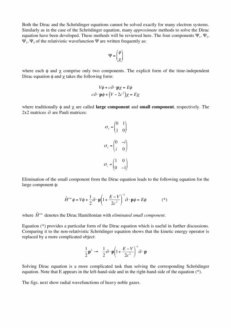
Both the Dirac and the Schrödinger equations cannot be solved exactly for many electron systems. Similarly as in the case of the Schrödinger equation, many approximate methods to solve the Dirac equation have been developed. These methods will be reviewed here. The four components Ψ1, Ψ2, Ψ3, Ψ4 of the relativistic wavefunction Ψ are written frequently as:

!

" =#

$

%

& ' (

) *

where each φ and χ comprise only two components. The explicit form of the time-independent Dirac equation φ and χ takes the following form:

!

V" + cr # $p% = E"

cr # $p" + V & 2c 2( )% = E%

where traditionally φ and χ are called large component and small component, respectively. The 2x2 matrices

!

r " are Pauli matrices:

!

"x

=0 1

1 0

#

$ %

&

' (

!

" y =0 #i

i 0

$

% &

'

( )

!

"z

=1 0

0 #1

$

% &

'

( )

Elimination of the small component from the Dirac equation leads to the following equation for the large component φ:

!

ˆ H esc" = V" +

1

2

r # $p 1+

E %V

2c2

&

' (

)

* +

%1

r # $p" = E" (*)

where

!

ˆ H esc denotes the Dirac Hamiltonian with eliminated small component.

Equation (*) provides a particular form of the Dirac equation which is useful in further discussions. Comparing it to the non-relativistic Schrödinger equation shows that the kinetic energy operator is replaced by a more complicated object:

!

1

2p2 "

1

2

r # $p 1+

E %V

2c2

&

' (

)

* +

%1r # $p

Solving Dirac equation is a more complicated task than solving the corresponding Schrödinger equation. Note that E appears in the left-hand-side and in the right-hand-side of the equation (*). The figs. next show radial wavefunctions of heavy noble gazes.

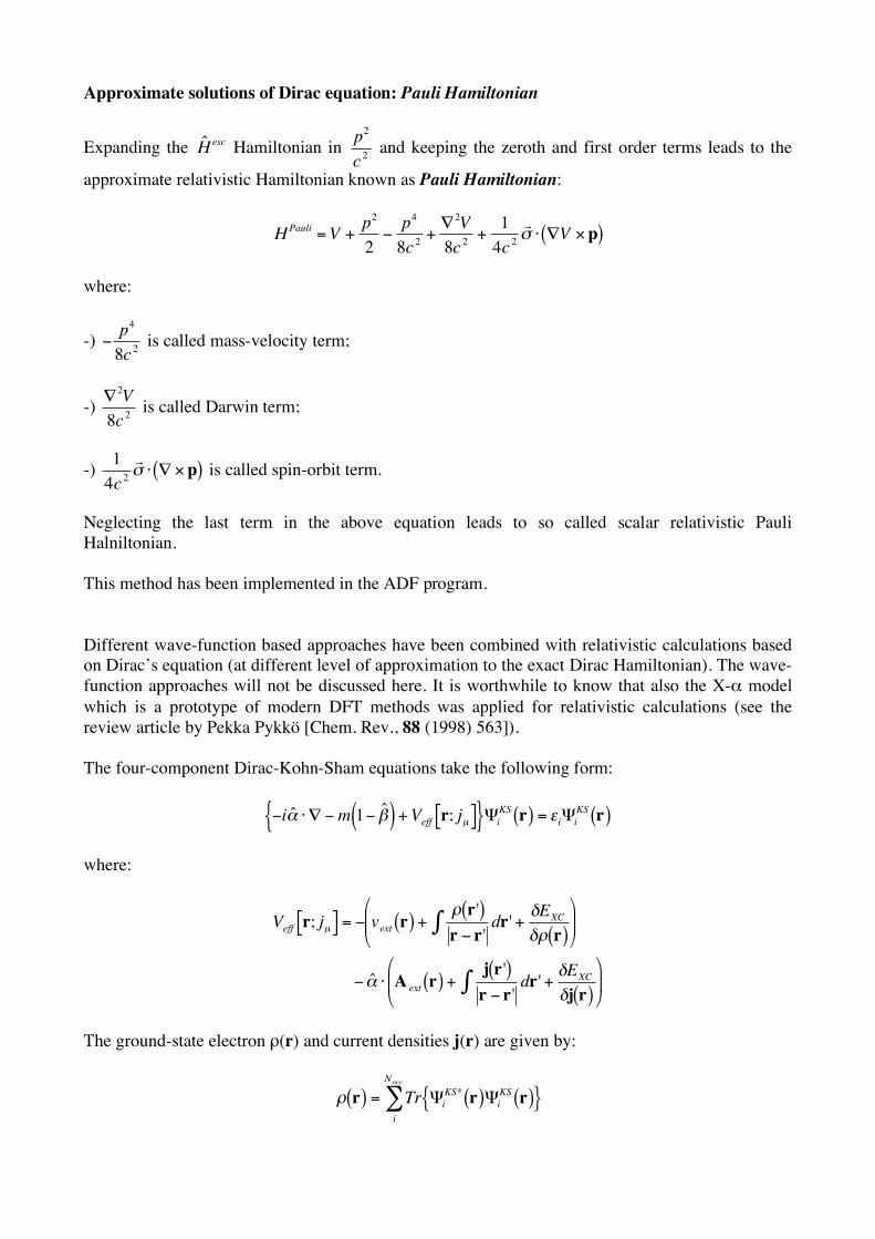
Approximate solutions of Dirac equation: Pauli Hamiltonian

Expanding the

!

ˆ H esc Hamiltonian in

!

p2

c2

and keeping the zeroth and first order terms leads to the

approximate relativistic Hamiltonian known as Pauli Hamiltonian:

!

HPauli =V +

p2

2"p4

8c2

+#2V

8c2

+1

4c2

r $ % #V &p( )

where:

-)

!

"p4

8c2

is called mass-velocity term;

-)

!

"2V

8c2

is called Darwin term;

-)

!

1

4c2

r " # $ %p( ) is called spin-orbit term.

Neglecting the last term in the above equation leads to so called scalar relativistic Pauli Halniltonian. This method has been implemented in the ADF program. Different wave-function based approaches have been combined with relativistic calculations based on Dirac’s equation (at different level of approximation to the exact Dirac Hamiltonian). The wave-function approaches will not be discussed here. It is worthwhile to know that also the X-α model which is a prototype of modern DFT methods was applied for relativistic calculations (see the review article by Pekka Pykkö [Chem. Rev., 88 (1998) 563]). The four-component Dirac-Kohn-Sham equations take the following form:

!

"i ˆ # $ % "m 1" ˆ & ( ) +Veff r; jµ[ ]{ }'i

KSr( ) = (i'i

KSr( )

where:

!

Veff r; jµ[ ] = " vext r( ) +# r'( )r " r'

dr'$ +%EXC

%# r( )

&

' (

)

* +

" ˆ , - A ext r( ) +j r '( )r " r'

dr'$ +%EXC

%j r( )

&

' (

)

* +

The ground-state electron ρ(r) and current densities j(r) are given by:

!

" r( ) = Tr #i

KS*r( )#i

KSr( ){ }

i

Nocc

$

and

!

jkr( ) = Tr "

i

KS* r( ) ˆ # k"i

KS r( ){ }i

Nocc

$

where

!

"i

KSr( ) denote the relativistic Dirac-Kohn-Sham orbitals.

Note that, the relativistic exchange-correlation potential depends not only on the electron and spin densities, but it depends on four current densities (electron density, spin-density, and orbital current density in the non-relativistic limit) [Rajagopal and Callaway, Phys. Rev. B, 7 (1973) 1912]. The good approximation for the relativistic exchange-correlation can be obtained by considering the non-relativistic exchange-correlation functional as a leading term and adding corrections due to magnetic interactions and retardation (Breit interactions) [Rajagopal and Ramana, Adv. Chem. Phys., 54 (1983) 231]. The leading term has the non-relativistic form:

!

EXC

",s[ ] = "#XC

",s( )$ dr where the spin density is obtained from the relativistic four-component wavefunction:

!

s = "i

r # "

i

i

Nocc

$ 1 %i

r # %

i

i

Nocc

$

where φi and χi are the large and the small component of the relativistic four component wave-function Ψ. Approximate solutions of Dirac equation: CPD Hamiltonian (ZORA) Chang, Pélisier, and Durand [Phys.Scr., 34 (1986) 394] derived another expansion of the

!

ˆ H esc . In

its zero-th order, the Hamiltonian takes the form:

!

H0 =V +

r " #p

c2

2c2$V

r " #p

=V + pc2

2c2$V

p+c2

2c2$V

r " # %V &p( )

The same zero-th order term has been derived by van Lenthe, Baerends, and Snijders [J.Chem.Phys., 99 (1993) 4597]. It is known as ZORA (Zeroth Order Regular Approximation) approach. This approach is currently implemented in the ADF program. The last term in the above equation is the spin-orbit term. Neglecting it leads to a scalar equation (scalar-ZORA). The following paper illustrates the significance of this term in closed-shell relativistic molecules [J. Chem.Phys., 105 (1996) 6505]. Relativistic Effective Core Potentials (ECP) Exact and approximate solutions of the Dirac equation show invariably that the s-orbitals of relativistic atoms shrink and their orbital energies are lowered compared to their hypothetic non-relativistic counterparts.

We recall now the concept of pseudopotentials discussed elsewhere [Phys. Rev., 116 (1959) 287]. Pseudopotentials make it possible to separate the core and the valence electrons. One can use the relativistic calculations to obtain s orbitals of the core and then apply usual non-relativistic Schrodinger equation in its pseudopotential formulation for remaining electrons. See for example the work of Kahn, Hay and Cowan [J. Chem. Phys., 68 (1978) 2386]. The concept of pseudopotentials is, therefore, very useful for relativistic elements. The most 'relativistic' electrons are removed from the problem. The relativistic effective core potentials are also applied within the Kohn-Sham formalism. According to Prof. Pekka Pykkö, in 90% of cases relativistic ECP provide an adequate theoretical approach to obtain the geometry and electronic structure of complexes involving relativistic elements.

Magnetic effects in atomic structure

Interaction with an external magnetic field : ZEEMAN Effect. We consider here the electronic Zeeman effect. However, since many nuclides have non-zero intrinsic spin, the same interaction occur with an external field. The magnitude of this interaction is, however, several (3-4) orders of magnitude smaller. Hamiltonian:

) H Ze =

r µ !

r H

r µ : magnetic dipole moment

r H : magnetic field

Contribution to the angular momentum:

-

S

e-

r µ L =

r I !S

current:

r I = !e

r " = !e

r v

2#r

surface: S = !r2

r µ L =

r I !S = "e

r v

2#r

$ %

& ' ! #r

2( ) ="e

r v r

2cemu[ ]

But

r p L = m

r v r

thus

r µ L =

!e

2mc

" #

$ % r p L

in quantum mechanics:

r p L ! "ih

) L

thus

r µ L =

eh

2mc

) L = !e

) L

Spin contribution

r µ S = ge!e

) S

ge = 2.0023 gyromagnetic factor of electron Thus, the Zeeman hamiltonian

) H Ze reads:

) H Ze = !e

) L + ge

) S ( ) "

r H

For nuclei with a nuclear spin, the complete Zeeman hamiltonian

!

ˆ H Ze

tot is thus:

!

ˆ H Ze

tot = "eˆ L + ge

ˆ S ( ) #r H $ gN"N

ˆ I #r H

Where gN and

!

"N

=eh

2Mc are respectiveely the gyromagnetic factor and the Bohr magneton of the

nucleus.

Paramagnetic susceptibility : Van Vleck’s formula This formula describes the dependence of the magnetic susceptibility χ(T),i.e. the proportionality factor between the bulk magnetisation and the external magnetic field, as a function of temperature and is the basis for the whole magnetochemistry. Consider the energy En of the n-th electronic level of an ion or complex molecule in an external magnetic field H and suppose that En can be expanded in a Taylor series as: En = En

(0) + En(1)H + En

(2)H2 + ... where En

(0) is the energy in absence of a magnetic field and where En(1) and En

(2) the 1st and 2nd order Zeeman coefficients respectively. To each level n, Van Vleck associates a magnetic moment µn, defined as:

µn = - !En

!H

The total magnetic moment M, i.e. the bulk magnetisation, is obtained in supposing that the levels n are populated according to a Boltzmann distribution, that is:

M =

N µn exp - En

kT!n

exp - En

kT!n

where k denotes the Boltzmann constant, T the temperature and N the Avogadro number. If H is sufficiently small, we can approximate:

exp - En

kT ! exp -

En(0)

kT 1-

En(1)H

kT

M reads then:

M =

N - En(1) - 2 En

(2)H 1- En

(1)H

kT exp -

En(0)

kT!n

1- En

(1)H

kT exp -

En(0)

kT!n

For H = 0, M must vanish when the moelcule or atom has no permanent magnetic moment, thus :

En(1) exp -

En(0)

kT!n

= 0

Keeping in the expression for M only terms linear in H, we can express the paramagnetic susceptibility as : ! =

M

H

which is nothing but Van Vleck formula:

! =

N En

(1) 2

kT - 2 En

(2) exp - En

(0)

kT!n

exp - En

(0)

kT!n

describing the temperature dependence of χ as a function of temperature. Due to the approximation of the exponential function for small arguments, the formula above might loose his validity say below 10K. The coefficients En(1) et En(2) can easily be obtained from perturbation theory. Indeed, let |n> be the wave function associated to level n and adapted to the perturbation

!

ˆ µ "r H , we get:

En

(1) = n | µ | n and

En(2)

=m | µ | n

2

En(0)

- Em(0)!

m!n

the sumation in the latter expression is restricted to indices m such that En

(0) ! Em(0).

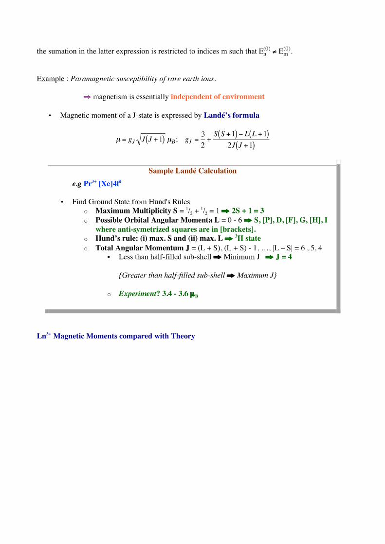
Example : Paramagnetic susceptibility of rare earth ions.

⇒ magnetism is essentially independent of environment

• Magnetic moment of a J-state is expressed by Landé’s formula

!

µ = gJ J J +1( ) µB; gJ =3

2+S S +1( ) " L L +1( )

2J J +1( )

Sample Landé Calculation e.g Pr3+ [Xe]4f2

• Find Ground State from Hund's Rules o Maximum Multiplicity S = 1/2 + 1/2 = 1 ⇒ 2S + 1 = 3 o Possible Orbital Angular Momenta L = 0 - 6 ⇒ S, [P], D, [F], G, [H], I

where anti-symetrized squares are in [brackets]. o Hund’s rule: (i) max. S and (ii) max. L ⇒ 3H state o Total Angular Momentum J = (L + S), (L + S) - 1, …, |L – S| = 6 , 5, 4

Less than half-filled sub-shell ⇒ Minimum J ⇒ J = 4

{Greater than half-filled sub-shell ⇒ Maximum J}

o Experiment? 3.4 - 3.6 µB

Ln3+ Magnetic Moments compared with Theory

Fig. Paramagnetic susceptibility of rare earth ions ;

!

µ =3kT"

N# 2is actually plotted.

---- ground level only, ---- including excited levels; ▴ experiment. Exercice : Repeat this example using the methods of chap. II. Kramers degeneracy In the absence of an external magnetic field, molecules with unpaired electrons (odd number of electrons) are at least two-fold degenerate. This is a fundamental theorem of quantum chemistry which traces back to time reversal symmetry.

Appendix 1: The Dirac Equation One of the first attempts at a relativistic quantum mechanical wave equation was the Klein-Gordon equation. Though it is theoretically sound from the perspective that it is consistent with both classical quantum mechanics and the special theory of relativity, it has several unsavory features which keep it from being a very powerful tool in relativistic quantum mechanics. Dirac later developed his own relativistic wave equation which did not have some of the shortcomings of the Klein-Gordon equation and that some of the supposed ‘‘errors’’ that the KG equation gave rise to were actually illustrating some new physics. The Dirac equation is only rigorous for a one particle system, but has been used as a starting point for a number of approximate many electron methods. 1.1 Klein-Gordon Equation The special-relativistic expression for the kinetic energy may be used to form the classical free particle Hamiltonian

!

E = c m2c2 + p

2[ ]1 2

(1.1) The analogous quantum mechanical expression may be constructed by replacing the classical momentum, p, with its quantum mechanical operator,

) p which yields the free particle wave equation

ih!

!t

"

# $

%

& ' ( = c m

2c

2+

) p

2( )1 2)

* + , - . ( (1.2)

This equation, however, does not satisfy some of the conditions required by special relativity. The wave equation is not invariant to a Lorentz transform, and the square root term introduces ambiguity. The Klein-Gordon equation, first proposed in 1927 rectifies both of these problems simply by taking the square of the original energy expression and extending the result to a quantum mechanical wave equation:

E2! = ih

"

"t

#

$ %

&

' (

2

! = m2c

4+

) p

2c

2( )! (1.3)

The resulting wave equation is Lorentz invariant and well defined, but suffers from other problems. Negative energy solutions to this equation are possible, which do not have a readily obvious explanation, and the probability density, ψ∗ψ, fluctuates with time as does its integral over all space. The foibles of the Klein-Gordon equation may make it a poor equation for the electron, but those weaknesses helped to point Dirac in the right direction and to develop a single particle equation which successfully surmounted all these problems. 1.2 Dirac’s Free Particle Equation In order for a wave equation to satisfy the special relativistic requirement of Lorentz invariance, derivatives in space and time must all appear in the same order. The K-G equation illustrates that an expression which satisfies this condition but is non-linear in the space and time derivatives gives rise to anomalous results. Dirac set out to find an equation which was first order in space and time derivatives. The result of his efforts, the Dirac equation, is difficult to motivate, impossible to prove, and far more complicated that the non-relativistic analog. However, Dirac’s wave equation for a single particle satisfies all the requirements of special relativity and quantum mechanics, and is able to predict the properties of one particle systems with remarkable accuracy.

Dirac’s equation for an electron in field-free space is given by

) p 0 ! " #

) p ! $mc( )% = 0 (1.4

where

) p 0 = i

h

c

!

!t (1.5)

and

) p is simply the three component momentum. In order to determine the nature of the three

components of α and β, it is useful to compare the modified equation

) p 0 ! " #

) p ! $mc( )* )

p 0 ! " #) p ! $mc( )% = 0 (1.6)

to the Klein-Gordon equation. Equations (1.3) and (1.6) are equivalent if we enforce the conditions

!i,! j[ ]+= !i! j + ! j! i = "ij (1.7)

where αi represents β for i=0 and αx, αy, and αz for i = 1, 2 and 3, respectively. In order for this set of four objects to fulfill these anti-commutation relations, each α must be, minimally, four-dimensional. One set of matrices which obey similar anti-commutation relations are the Pauli spin matrices: σx,y,z. These are 2x2 matrices, however, and there are only three of them, so they are not useful in their usual form. If the α’s are defined as

!0 =12x2 0

0 "12x2

#

$ % %

&

' ( ( (1.8)

!i =0 " i" i 0

#

$ % %

&

' ( ( (1.9)

Where 12x2 is a two by two identity matrix and σi are the Pauli spin matrices:

!

"x

=0 1

1 0

#

$ %

&

' (

!

" y =0 #i

i 0

$

% &

'

( )

!

"z

=1 0

0 #1

$

% &

'

( )

Though these four by four matrices do not represent the only set of matrices which satisfy the anti-commutation relations, they may only differ by a similarity transform from this set. Because the Dirac equation contains operators represented by four dimensional matrices, the solutions {ψ} must be represented by a four component vector

! =

!1!2!3!4

"

#

$ $ $ $ $

%

&

' ' ' ' '

(1.10)

The interpretation of the components of this four-vector is not readily evident. Expressing the Dirac

equation in full matrix form provides some elucidation

) p 0 !mc( ) 0 !

) p z !

) p x ! i

) p y( )

0) p 0 !mc( ) !

) p x + i

) p y( ) )

p z

!) p z !

) p x ! i

) p y( ) )

p 0 + mc( ) 0

!) p x + i

) p y( ) )

p z 0) p 0 + mc( )

"

#

$ $ $ $ $ $

%

&

' ' ' ' ' '

(1

(2

(3

( 4

"

#

$ $ $ $ $

%

&

' ' ' ' '

= 0 (1.11)

The non-relativistic electronic wave-function has two components corresponding to the α and β components of spin angular momentum. In the non-relativistic limit, p0 approaches mc, and the terms which couple ψ1 with ψ2 drop out. What remains are four eigenvector equations, with approximate eigenvalues of +m0c2 for ψ1 and ψ2, and -m0c2 for ψ3 and ψ4. ψ1 and ψ2, then, may be interpreted as the α and β components of positive energy, electron-like solutions, but the solutions which are dominated by ψ3 and ψ4 do not possess a readily evident interpretation. Dirac deduced that these solutions correspond to a particle with the same mass as the electron but an opposite charge, and dubbed these particles positrons. Far from being figments of a theorist’s imagination, only three years after Dirac First suggested them in 1930, positrons were observed experimentally. 1.3 Hydrogenic Solutions of Dirac’s Equation In its present form, the Dirac equation cannot even address the hydrogen atom, since it has no provision for an external potential. If we introduce a scalar and vector potential, eφ+

r A , to the

momenta of the field free Dirac equation

!

p0" p

0#e$

c (1.12)

r p !

r p "

r A

c=

r # (1.13)

then the Dirac equation becomes

!

p0"e#

c"$ % & "'mc

(

) * +

, - . = 0 (1.14)

If the potential terms are not explicitly time dependent, we may make the rearrangement

!

"mc + c# $ % + e&[ ]' = E' (1.15) The left hand side defines the Dirac Hamiltonian for a single particle in a time-independent electro-magnetic field. In the absence of a magnetic field the Dirac Hamiltonian,

) H p , may be expressed in

full matrix form as

!

) H p =

e" + mc2( ) 0 c

) p z c

) p x # i

) p y( )

0 e" + mc2( ) c

) p x + i

) p y( ) #c

) p z

c) p z c

) p x # i

) p y( ) e" #mc

2( ) 0

c) p x + i

) p y( ) #c

) p z 0 e" #mc

2( )

$

%

& & & & &

'

(

) ) ) ) )

(1.16)

This Hamiltonian is now ready to take on the task of an electron in the field of a nucleus. Because of the spherical symmetry of the nuclear potential, the Schrödinger equation for the hydrogenic atom may be simplified via separation of variables into a radial equation and two angular equations. The angular solutions are given by the spherical harmonics, Ylml !,"( ) , and the

radial solutions by

Rnl r( ) = Nnle!r

na 02r

na0

"

# $ $

%

& ' '

l

Ln +l2l+1 2r

na0

"

# $ $

%

& ' ' (1.17)

where Ln + l

2l+1x( ) are the associated Laguerre polynomials, and n, l, and ml are the principal quantum

number, orbital angular momentum quantum number, and the z-projection of l, respectively. The hydrogenic solutions to the Dirac equations may also be achieved analytically, though the resulting eigenfunctions cannot be so simply expressed. Because of the presence of the

) ! "

) p term,

the ) s and

) l operators do not commute with

) H . The components of the

) j =

) l +

) s operator,

however, does commute with

) H , and so the eigenfunctions of the Hamiltonian may be

eigenfunctions of

) j 2 and

) j z ,

) l

2 and ) s

2 also commute with the Hamiltonian, and so we may still associate a particular l and s value with each solution, ψ. It is useful, at this point, to express the four-component wave-function as a pair of two component spinors, φ and θ:

! =

!1!2!3!4

"

#

$ $ $ $ $

%

&

' ' ' ' '

=(

)

"

# $ %

& ' (1.18)

Such a separation is dictated by the nature of the 4x4 Pauli spin matrices, and makes it possible to work with the familiar two-spinors of non-relativistic theory. Capitalizing on the commutation of

) H

with

) j , each spinor may be expressed as the product of a two-component eigenfunction of

) j which

is dependent upon the spin and spatial angular coordinates and a radial function: ! = g r( )"l

j,m j; # = f r( )"l

j,m j (1.19) The eigenfunctions of

) j , !l

j,m j , may be expressed as sums of direct products of the more familiar eigenfunctions of

) l and

) s and the appropriate Clebsh-Gordon coefficients:

!lj= l+1 2( ),m j

= ! j,m j

+( )=

l +mj +1 2

2l +1Yl,m j"1 2

#1 21 2( ) +

l "mj +1 2

2l +1Yl,mj +1 2

#1 2"1 2( ) (1.20)

!lj= l"1 2( ),m j

= ! j,m j

"( )= "

l "mj +1 2

2l +1Yl,m j"1 2

#1 21 2( ) +

l +mj + 1 2

2l +1Yl,m j+1 2

#1 2"1 2( ) (1.21)

where Yl,m j±1 2

are the spherical harmonics and

!1 21 2

= " =1

0

#

$ % &

' ( ; !)1 2

1 2= * =

0

1

#

$ % &

' ( (1.22)

Next, it is useful to define the operator

) K = ! "

) l +1( ) (1.23)

which commutes with ) J . The eigenvalue equation associated with

) K is given by

) K ! j,m j

±( )=± k!j,m j

±( ) (1.24) where

!

k =j +1 2 if j = l "1 2

" j +1 2( ) if j = l +1 2

# $ %

(1.25)

Because of the spherical symmetry of the nuclear potential, the eigensolutions may be further separated on the basis of their response to spatial coordinate inversion. The parity operator commutes with the full Hamiltonian, and so the final eigenfunctions, ! j,m j

, must also obey the eigenvalue equation !" # r( ) = ±" r( ) (1.26) This necessarily dictates one of the following forms for the four-component eigensolutions:

! j,m j

+( )=g r( )" +( )

f r( )" #( )

$

% & &

'

( ) ) (1.27)

or

! j,m j

"( )=

"g r( )# "( )

f r( )# +( )

$

% & &

'

( ) )

(1.28)

It is possible, through the use of the identity

!

" #) p $ " #

) r ( )

) r #

) p +

" #) l

r

%

& '

(

) * (1.29)

and the property

! "

) r ( )# j,m j

±( )= $# j,m j

m( ) (1.30) to completely separate out the angular functions from the eigenvalue equation, and thereby achieve two coupled, complex differential equations for the radial functions f(r) and g(r). The resultant equations are greatly simplified by the substitutions

f(r) = F(r)/r and g(r) = iG(r)/r (1.31) to yield

!

mc2" E " Z r( )F r( ) " c

dG r( )dr

" kcG r( ) r = 0 (1.32)

!

"mc2" E " Z r( )F r( ) + c

dG r( )dr

" kcG r( ) r = 0 (1.33)

The solutions to these differential equations may be determined by first solving the asymptotic equations in the limit as

!

r"# . These solutions, which are of the form

!

F r( ) = 1+ E mc2exp "

mc 1" E mc2( )2

hr

#

$

% % %

&

'

( ( ( (1.34)

!

G r( ) = 1" E mc2exp "

mc 1" E mc2( )2

hr

#

$

% % %

&

'

( ( ( (1.35)

are then multiplied by an undetermined power series for both components and the bound state solutions are sought. The final form of each wave-function is uniquely determined by the recursive relations of the power series and the boundary conditions, but may not be expressed in a simple general form. The resulting electronic energies are given by

!

En = mc 2 1+Z"( )

2

n # j #1 2 + j +1 2( )2

+ Z"( )2$

% &

' ( ) 2

*

+

, , , ,

-

.

/ / / /

#1 2

(1.36)

where α is the fine structure constant, and is given by

!

1 c in atomic units. The four-component nature of the Dirac eigenfunctions gives rise to many interesting differences when compared to the non relativistic solutions. In order to better understand these differences, it is useful to inspect some simple approximations of the lowest energy hydrogenic solutions, for example the n = 2, j = {1/2, 3/2} solutions.

!

n = 2, j =1 2, k =1,m j =1 2( )

1

2 2

e"# 2

1" # 2( )0

i

2Z$e"# 2

1" # 4( )cos%

i

2Z$e"# 2

1" # 4( )sin%ei&

'

(

) ) ) ) ) )

*

+

, , , , , ,

(1.37)

!

n = 2, j =1 2, k =1,m j = "1 2( )

1

2 2

0

e"# 2

1" # 2( )i

2Z$e"# 2

1" # 4( )sin%ei&

"i

2Z$e"# 2

1" # 4( )cos%

'

(

) ) ) ) ) )

*

+

, , , , , ,

(1.38)

!

n = 2, j =1 2, k = "1,m j =1 2( )

1

4 6

e"# 2#cos$

e"# 2# sin$ei%

"3i

2Z&e"# 2

1" # 6( )

0

'

(

) ) ) ) )

*

+

, , , , ,

(1.39)

!

n = 2, j =1 2, k = "1,m j = "1 2( )

1

4 6

e"# 2#cos$

e"# 2# sin$ei%

0

"3i

2Z&e"# 2

1" # 6( )

'

(

) ) ) ) )

*

+

, , , , ,

(1.40)

!

n = 2, j = 3 2, k = 2,m j = 3 2( )

1

8

e"# 2

sin$ei%

0i

4Z&e"# 2

1" # 4( )sin$ cos$ei%

i

4Z&e"# 2

1" # 4( )sin2$e2i%

'

(

) ) ) ) ) )

*

+

, , , , , ,

(1.41)

!

n = 2, j = 3 2, k = 2,m j = "3 2( )

1

8

0

e"# 2

sin$ei%

i

4Z&e"# 2

1" # 4( )sin2$e2i%

"i

4Z&e"# 2

1" # 4( )sin$ cos$ei%

'

(

) ) ) ) ) )

*

+

, , , , , ,

(1.42)

!

n = 2, j = 3 2, k = 2,m j =1 2( )

1

4 3

e"# 2

sin$ei%

"1

2e"# 2

sin$ei%

"i

8Z&e"# 2# 1" 3cos2$( )

3i

8Z&e"# 2# sin$ cos$ei%

'

(

) ) ) ) ) )

*

+

, , , , , ,

(1.43)

!

n = 2, j = 3 2, k = 2,m j = "1 2( )

1

4 3

1

2e"# 2

sin$ei%

e"# 2

sin$ei%

3i

8Z&e"# 2# sin$ cos$ei%

i

8Z&e"# 2# 1" 3cos2$( )

'

(

) ) ) ) ) )

*

+

, , , , , ,

(1.44)

These solutions are correct to order Zα, as illustrated in Moss's discussion of the hydrogenic solutions to Dirac's equation [R. E. Moss, Advanced Molecular Quantum Mechanics (John Wiley and Sons, New York, 1973).]. Here, analogous to the non-relativistic case, for each unique combination of the principal quantum number n and a specific angular momentum quantum number j, the solutions must be further classified according to the projection of their total angular momentum on the z-axis, mj. These solutions are, of course, degenerate in the absence of an external field. The contributions from the first two components of the wave-function tend to be much larger than the contributions from the final two components for electron-like solutions. For this reason the upper two-component spinor is known as the large component of the wave-function, while the lower spinor is known as the small component. By orthogonality, the opposite is true for the positron-like solutions. Since the angular and spin portions of the wave-functions are normalized, the magnitude of the large and small contributions is determined entirely by the radial functions, f(r) and g(r). Given the asymptotic form of the radial equations (1.34) and the orbital energy (1.36), the ratio of their contributions may be expressed as

g r( )

f r( )!Z"

2n (1.45)

In general, the ratio will probably be larger than this approximate value in regions close to the nucleus, where the contribution of g(r) is the greatest. The contribution of the small component, then, may be significant for sufficiently heavy nuclei. Though hydrogenic ions with very heavy nuclei may not be of great practical interest, this relationship will have implications for heavy many-electron atoms where the innermost electrons experience a large portion of the full nuclear charge and hence are closely related to the analogous hydrogenic systems. One interesting consequence of the four-component wave-function may be observed in the associated probability density. Scalar wave-functions, ψ, which possess radial and angular nodes will have the same radial and angular nodes in their probability density, ψ∗ψ. The four-component wave-function, however, gives rise to a probability density which sis the sum of the probability densities associated with the large and small wave-functions, φ and χ, respectively. The radial component of φ and χ, possess different numbers of nodes and, in general, none of these nodes will coincide. Similarly, the angular contributions of φ differ from those of χ by a single unit of angular momentum. Therefore, although φ∗φ and χ∗χ may possess either radial of angular nodes individually, their sum, their sum will be node-less. The energy eigenvalues of the hydrogenic solutions to the Schrödinger equation are only dependent upon n, the principal quantum number, while the Dirac hydrogenic eigenvalues are dependent on both n and j. The spectral dependence on j is upheld by experimental observation, however the degeneracy of eigenvalues for solutions with the same j values but differing l values is not observed in nature. The breaking of this degeneracy is known as the Lamb shift and its origin has been attributed to the difference in the interaction of the different j eigenfunctions with the vacuum fluctuations predicted by quantum electrodynamics. The magnitude of the Lamb shift is much

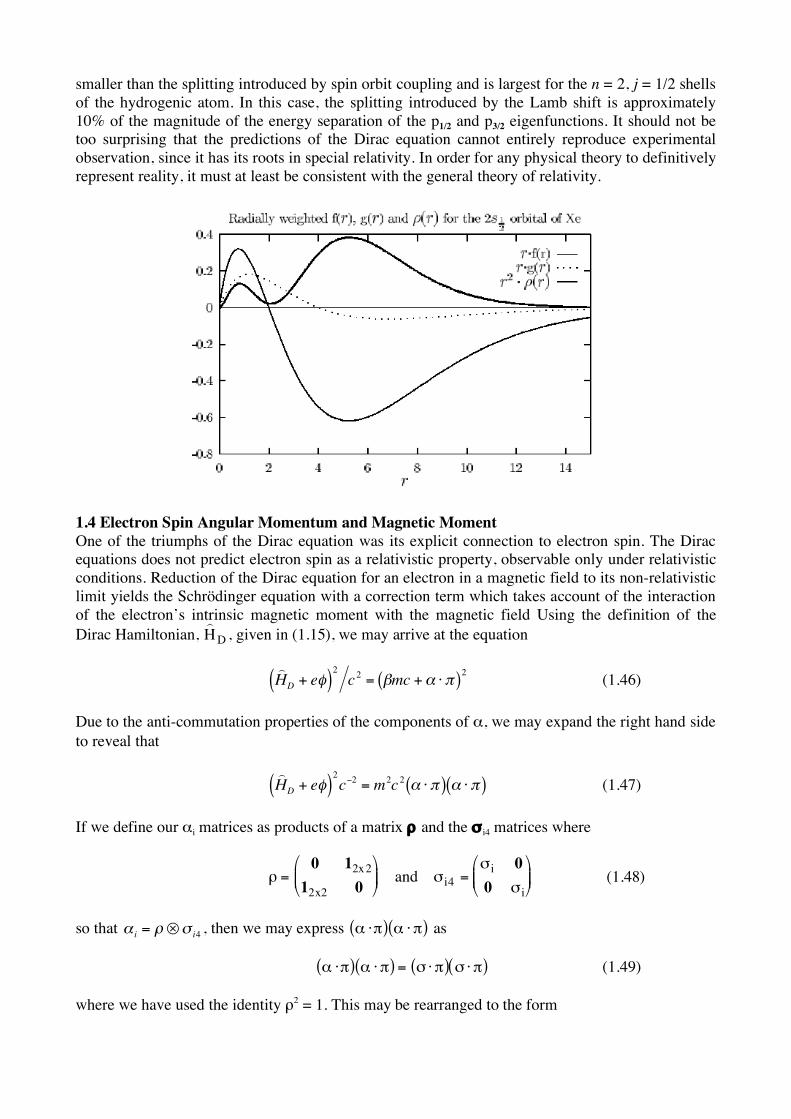
smaller than the splitting introduced by spin orbit coupling and is largest for the n = 2, j = 1/2 shells of the hydrogenic atom. In this case, the splitting introduced by the Lamb shift is approximately 10% of the magnitude of the energy separation of the p1/2 and p3/2 eigenfunctions. It should not be too surprising that the predictions of the Dirac equation cannot entirely reproduce experimental observation, since it has its roots in special relativity. In order for any physical theory to definitively represent reality, it must at least be consistent with the general theory of relativity.

1.4 Electron Spin Angular Momentum and Magnetic Moment One of the triumphs of the Dirac equation was its explicit connection to electron spin. The Dirac equations does not predict electron spin as a relativistic property, observable only under relativistic conditions. Reduction of the Dirac equation for an electron in a magnetic field to its non-relativistic limit yields the Schrödinger equation with a correction term which takes account of the interaction of the electron’s intrinsic magnetic moment with the magnetic field Using the definition of the Dirac Hamiltonian,

) H

D, given in (1.15), we may arrive at the equation

!

) H

D+ e"( )

2

c2 = #mc +$ % &( )

2 (1.46) Due to the anti-commutation properties of the components of α, we may expand the right hand side to reveal that

!

) H

D+ e"( )

2

c#2 = m

2c2 $ % &( ) $ % &( ) (1.47)

If we define our αi matrices as products of a matrix ρ and the σ i4 matrices where

! =0 12x2

12x2 0

"

# $ $

%

& ' ' and ( i4 =

( i 0

0 ( i

"

# $ $

%

& ' ' (1.48)

so that

!

"i= # $%

i4, then we may express ! "#( ) ! " #( ) as

! "#( ) ! " #( ) = $ " #( ) $ " #( ) (1.49) where we have used the identity ρ2 = 1. This may be rearranged to the form

! " #( ) ! " #( ) = #" # + i! # $ #( ) (1.50) via sundry vector identities. The cross-product of π with itself does not drop out. This is because πi is the sum of two vectors, p and A, so the cross terms of the cross products remaining, making the cross-product of π with itself ! " !( ) = #ih$ "A = #ihB (1.51) Returning to our original equation (1.39), we may make this substitution to arrive at

!

) H

D+ e"( )

2

c#2 = m

2c2 + $ 2 + h%

4B (1.52)

In the non-relativistic limit this gives us an Hamiltonian of the form

!

) H

D= "e# +

$ 2

2m+

h

2m%B (1.53)

The final term indicates that a term which corresponds to a body with a magnetic moment of

!h

2m" in a magnetic field B must be added to give the proper energy. This prediction of electron

spin as a property which should exist in the non-relativistic limit provides strong evidence that Dirac's equation provides a more complete physical picture than the wave equation of Schrödinger, where electron spin must be treated in an ad hoc manner