Embed Size (px)
Citation preview
acta physica slovaca vol. 60 No. 3, 259 – 391 June 2010
RELATIVISTIC EFFECTS IN ATOMIC AND MOLECULAR PROPERTIES ∗
Miroslav Ilias,a,1 Vladimır Kello,b,2 Miroslav Urbanb,c,3aDepartment of Chemistry, Faculty of Natural Sciences, Matej Bel University, Tajovskeho 40,
SK–974 00 Banska Bystrica, SlovakiabDepartment of Physical and Theoretical Chemistry, Faculty of Natural Sciences, Comenius
University, Mlynska dolina, SK–842 15 Bratislava, Slovakiac Slovak University of Technology in Bratislava, Faculty of Materials Science and Technology
in Trnava, Institute of Materials Science, Bottova 25, SK–917 24 Trnava, Slovakia.
Received 17 May 2010, accepted 1 June 2010
This paper is dedicated to the memory of our friend, prof. Andrzej J. Sadlej, with whom we had aprivilege and pleasure to collaborate for decades in many areas of theoretical and computationalchemistry. We are particularly indebted to Andrzej for introducing us to the area of relativisticeffects and their importance in atomic and molecular properties. Senior authors will rememberforever days and nights of joint work and discussions on chemistry, physics and life.
We present an overview of basic principles and methods of the relativistic quantum chemistry.Practical aspects of different methods will be discussed stressing their capability of providingaccurate predictions of molecular properties, particularly in species containing a heavy metalelement. We will present a series of examples showing the importance of relativistic effectsin a variety of molecular properties including electron affinities, ionization potentials, reac-tion and dissociation energies, electric, spectroscopic and other properties. It is possible torecognize a link between these properties and behaviour of materials in some cases. Particu-lar attention is paid to relativistic calculations of the nuclear quadrupole moments for whichaccurate theoretical electric field gradient is combined with data from the microwave spec-tra. Important aspect of the present paper is understanding of trends in electronically relatedatoms throughout the Mendeleev Periodic Table rather than focusing on highly accurate num-bers. We will show that relativistic effects represent an unavoidable instrument for explainingsome unexpected properties of heavy metal containing compounds. We will also discuss aninterplay between the many–electron correlation and relativistic effects.
DOI: 10.2478/v10155-010-0003-1
PACS: 31.15.A-, 31.15.aj, 31.15.ap, 31.15.bw, 31.15.V-, 31.30.jc, 31.30.jp, 32.10.Hq
KEYWORDS:
Relativistic effects, Electron correlation, Change of picture, Ionizationpotentials, Electron affinities, Excitation energies, Dipole moments andpolarizabilities, Electric field gradients, Nuclear quadrupole moments,Multiple bonds, Intermolecular interactions, NMR.
∗The reference [71] was corrected by the authors after the paper had been printed out.1E-mail address: [email protected] address: [email protected] address: [email protected]; [email protected]
259

260 Relativistic effects in atomic and molecular properties
Contents
1 Introduction 262
2 Manifestation of relativistic effects on atomic properties. Basic notes. 2642.1 Z–dependence of the relativistic effects . . . . . . . . . . . . . . . . . . . . . . 269
2.1.1 Semi–classical estimate of spin–orbit effects . . . . . . . . . . . . . . . 271
3 Basic notes on nonrelativistic electronic structure methods for many–electron atomsand molecules 2743.1 Schrodinger equation and the hydrogen–like atoms . . . . . . . . . . . . . . . . 274
3.1.1 Angular momentum . . . . . . . . . . . . . . . . . . . . . . . . . . . . 2753.1.2 Spin momentum . . . . . . . . . . . . . . . . . . . . . . . . . . . . . . 275
3.2 Many-electron systems . . . . . . . . . . . . . . . . . . . . . . . . . . . . . . . 2773.2.1 The independent–electron model: The Hartree–Fock method . . . . . . . 2793.2.2 Algebraic approximation . . . . . . . . . . . . . . . . . . . . . . . . . . 2813.2.3 Electron correlation in the nonrelativistic theory of many electron systems 2823.2.4 Configuration interaction . . . . . . . . . . . . . . . . . . . . . . . . . . 2833.2.5 Coupled Cluster theory . . . . . . . . . . . . . . . . . . . . . . . . . . . 2853.2.6 CASSCF, RASSCF, and CASPT2 methods . . . . . . . . . . . . . . . . 293
4 Relativistic theory of many–electron atoms and molecules 2964.1 Lorentz transformations . . . . . . . . . . . . . . . . . . . . . . . . . . . . . . . 2964.2 Klein–Gordon equation . . . . . . . . . . . . . . . . . . . . . . . . . . . . . . . 2974.3 Dirac equation . . . . . . . . . . . . . . . . . . . . . . . . . . . . . . . . . . . . 297
4.3.1 Nonrelativistic limit of the Dirac equation . . . . . . . . . . . . . . . . . 2994.3.2 Solution of the Dirac equation for the hydrogen–like atom . . . . . . . . 3014.3.3 Finite nucleus . . . . . . . . . . . . . . . . . . . . . . . . . . . . . . . . 303
4.4 Four component relativistic quantum chemistry . . . . . . . . . . . . . . . . . . 3044.4.1 The relativistic electron–electron interaction . . . . . . . . . . . . . . . . 3044.4.2 The Dirac–Coulomb–Breit/Gaunt Hamiltonian . . . . . . . . . . . . . . 3054.4.3 The Dirac–Hartree–Fock method . . . . . . . . . . . . . . . . . . . . . 3064.4.4 Symmetry aspects . . . . . . . . . . . . . . . . . . . . . . . . . . . . . 3074.4.5 Classification of relativistic electronic states of atoms and molecules . . . 3084.4.6 Four–component relativistic basis set functions . . . . . . . . . . . . . . 309
4.5 Relativistic correlation methods . . . . . . . . . . . . . . . . . . . . . . . . . . 3104.5.1 Second–order Kramers restricted MP2 method . . . . . . . . . . . . . . 3114.5.2 Relativistic Coupled Cluster and Configuration Interaction methods . . . 312
4.6 Transformations to two–component Hamiltonians . . . . . . . . . . . . . . . . . 3124.6.1 Foldy–Wouthuysen transformation . . . . . . . . . . . . . . . . . . . . . 3134.6.2 Douglas–Kroll transformation . . . . . . . . . . . . . . . . . . . . . . . 3144.6.3 Exact decoupling . . . . . . . . . . . . . . . . . . . . . . . . . . . . . . 3154.6.4 Infinite order two–component Hamiltonian (IOTC) . . . . . . . . . . . . 318
4.7 Spin–orbit effects . . . . . . . . . . . . . . . . . . . . . . . . . . . . . . . . . . 3204.7.1 Mean–field spin–orbit operator . . . . . . . . . . . . . . . . . . . . . . . 322

CONTENTS 261
4.7.2 RASSI–SO . . . . . . . . . . . . . . . . . . . . . . . . . . . . . . . . . 3244.8 Fine effects, Lamb shift . . . . . . . . . . . . . . . . . . . . . . . . . . . . . . . 324
5 Relativistic effects in atoms and molecules, their properties and interactions 3265.1 Ionization potentials, electron affinities and excitation energies . . . . . . . . . . 328
5.1.1 Ionization potentials . . . . . . . . . . . . . . . . . . . . . . . . . . . . 3285.1.2 Electron affinities . . . . . . . . . . . . . . . . . . . . . . . . . . . . . . 3295.1.3 Excitation energies . . . . . . . . . . . . . . . . . . . . . . . . . . . . . 333
5.2 Relativistic effects on molecular geometries . . . . . . . . . . . . . . . . . . . . 3365.3 Electric properties – dipole moments and dipole polarizabilities . . . . . . . . . . 3385.4 Determination of nuclear quadrupole moments . . . . . . . . . . . . . . . . . . 345
5.4.1 Change of picture . . . . . . . . . . . . . . . . . . . . . . . . . . . . . . 3465.4.2 Examples of calculations . . . . . . . . . . . . . . . . . . . . . . . . . . 348
5.5 Dissociation and reaction energies . . . . . . . . . . . . . . . . . . . . . . . . . 3535.5.1 Quadruple, quintuple or sextuple bonds? . . . . . . . . . . . . . . . . . . 358
5.6 Intermolecular interactions . . . . . . . . . . . . . . . . . . . . . . . . . . . . . 3595.7 NMR properties of molecules . . . . . . . . . . . . . . . . . . . . . . . . . . . . 368
5.7.1 Four–component calculations of NMR shielding constants . . . . . . . . 3685.7.2 Gauge including atomic orbitals in the four–component theory . . . . . . 3705.7.3 Electron correlation in NMR calculations . . . . . . . . . . . . . . . . . 370
5.8 From relativistic effects in atoms and molecules to gas–phase properties and thecondensed phase . . . . . . . . . . . . . . . . . . . . . . . . . . . . . . . . . . 372
6 Conclusions 376
Acknowledgment 376
Appendix 377
References 378

262 Relativistic effects in atomic and molecular properties
1 Introduction
Until the seventies of the 20th century it was generally accepted that for a description of the elec-tronic structure of atoms and molecules and, therefore, for the whole chemistry and for the sub-stantial part of physics, relativistic theory is not needed. According to Sheldon L. Glashow [1],Nobel Prize Winner for Physics, 1979, ”Modern elementary–particle physics is founded upon thetwo pillars of quantum mechanics and relativity. I have made little mention of relativity so farbecause, while the atom is very much a quantum system, it is not very relativistic at all. Relativitybecomes important only when velocities become comparable to the speed of light. Electrons inatoms move rather slowly, at a mere of one percent of light speed. Thus it is that a satisfac-tory description of the atom can be obtained without Einstein’s revolutionary theory.” Possiblythese beliefs were initiated by Dirac himself [2], who wrote in 1929 that ”Relativistic effects aretherefore of no importance in the consideration of atomic and molecular structure and ordinarychemical reactions”. In the last thirty years the situation has changed considerably. Presently, itis generally accepted that relativistic effects must be considered in compounds containing heavymetal elements. Even understanding of the Mendeleev Periodic Table is impossible without uti-lizing the ideas of theory of relativity along, of course, with quantum physics. When talkingabout the relativistic theory of atoms and molecules we mean, of course, the special theory ofrelativity discovered by Einstein in 1905. It was in the same year in which he published thetheory of the photo–electric effect, which is one of pillars on which the quantum mechanicswas founded few years later. Therefore, both fundamental theories of the electronic structure ofatoms and molecules were discovered and developed about at the same time, in first few yearsof the twenties century. Quantum physics was accepted as a basic theory for understanding ofatomic and molecular properties almost immediately after its discovery. The first theory of thechemical bond formulated by Heitler and London in 1927 [3], is considered as the ”birthday”of quantum chemistry. Theory of relativity, however, was awaiting for recognition of its fun-damental importance in molecular physics and chemistry much longer. It took several decadesafter Dirac’s formulation of his fundamental relativistic quantum mechanics in 1928 [4] until histheory was developed as a tool for the treatment of many–electron molecular systems. Currently,it is generally accepted that both, quantum mechanics and the special theory of relativity, areessential in the description and understanding of molecular properties. Clearly, relativity is in-creasingly important for molecules containing an element with high atomic number. However,even accurate description of properties of the lightest hydrogen molecule, as performed by Kołosand Wolniewicz in 1961 [5] showed that careful treatment of relativistic effects is unavoidable.Solutions of the Dirac–Fock equations [6,7] for many–electron systems with atomic numbers upto 120 was presented by Desclaux in 1973 [8]. An important milestone on a long way towardsrecognizing the importance of the relativistic quantum theory in understanding general trends ofmolecular properties is a paper entitled ”Relativity and the Periodic System of elements” pub-lished by Pyykko and Desclaux in 1979 [9]. This work was followed by many other reviewson the development of the relativistic quantum theory and its applications in quantum molecularsciences by Pyykko, Kutzelnigg, Schwerdtfeger, Schwarz and other authors [10–22], to name atleast a few. A further development of relativistic quantum chemistry in molecular sciences wasgreatly affected by excellent books published recently, particularly Relativistic electronic struc-ture theory, Part 1. Fundamentals and Part 2. Applications, edited by Schwerdtfeger [23, 24]and books by Dyall and Fægri [25] and by Reiher and Wolf [26].

Introduction 263
The purpose of this review is a short description of basic nonrelativistic theories, includingmost important methods for treating the many–electron correlation problem. An essential part ofthis paper is devoted to a transparent overview of relativistic many–electron theories in which theelectron correlation problem (very difficult to treat accurately even at the nonrelativistic level)will be considered at the relativistic level. Rigorous four–component relativistic many–electroncalculations for larger molecules are hardly tractable in the spirit of the four–component Diracrelativistic quantum mechanics [4,27]. Approximate extensions applicable to many–electron sys-tems including electron correlation are feasible but very tedious. Methodologies which give riseto a variety of two–component Hamiltonians and allow treating larger molecular systems will bediscussed in more detail in Section 4 and specifically in Section 4.6. For practical purposes it isimportant to note that in many applications it is sufficient to consider relativistic effects even atthe no–pair one–component level. This is frequently denoted as ”scalar” relativistic level. Thisis a pragmatic attitude toward the many–electron correlated relativistic treatment of molecules.Great advantage is that scalar relativistic effects can be taken into account within common non-relativistic many–electron wave function methods, with only a small modification. One– andtwo–component methods are frequently called also as ”quasi–relativistic”. Spin–orbit (SO) ef-fects are neglected within the one–component framework but applications may go to as largemolecules as it is possible in the nonrelativistic case, still using sophisticated many–electronwave function methods. We will demonstrate this approach in many applications to problems inwhich spin–orbit effects are unimportant. A large part of relativistic quantum chemistry calcu-lations is performed using the density functional theory (DFT) which is applicable to truly largesystems, although the control of accuracy is to some extent questionable.
In comparison with scalar relativistic effects, rigorous four–component many–electron rel-ativistic theories employing sophisticated treatment of the electron correlation, like relativisticCoupled Cluster (CC) theories, are very tedious in most cases. Nevertheless, there is a largeprogress in making these theories (or their theoretically well founded approximations) applicableto a larger variety of systems of chemical and physical importance. We will pay attention to thesetheories and to their transformation to two–component treatments which are better applicable tolarger many–electron calculations still allowing sufficiently accurate treatment of spin–orbit ef-fects.
Somewhat out of the main scope of this review are fine structure problems, e.g., spectraof atoms and molecules, Lamb shift, Quantum Electron Dynamics (QED) effects to which paylarge attention some experts in relativistic many– electron theories. Of course, there exists a richliterature on QED effects in simple systems. Less is known about the importance of these effectson properties and reactivity of many–electron atoms and molecules. Presently, some resultsindicate that QED effects may eventually lead to interesting chemical and physical consequencesbut the knowledge in this area still remains quite limited [28, 29].

264 Relativistic effects in atomic and molecular properties
2 Manifestation of relativistic effects on atomic properties. Basic notes.
Historically, a breakdown in understanding of the chemical and physical behaviour of elementsand their compound goes back to the formulation of the periodic law and the Periodic Tableof elements by D. I. Mendeleev in 1869 [30]. The impact of his discovery on chemistry andmolecular physics can be hardly exaggerated. As the greatest (we believe) theoretical chemistin the history, Mendeleev was able to systematise the accumulated knowledge, to interpret thefacts and to predict chemical properties of elements and their compounds. Yet, he has failed inplacing some elements at proper positions. As we can see in Fig. 2.1, in which we reproduce theMendeleev Periodic Table from his 1869 paper published in Germany [31] which was abstractedfrom the original Russian paper [30], most elements have proper location. It corresponds to ourpresent knowledge of the isoelectronic valence electronic structure of elements belonging to thesame group in the Periodic Table. As we can see, incorrect location concerns in fact exclusively
Fig. 2.1. Mendeleev Periodic Table as published in 1869, Ref. [31].

Manifestation of relativistic effects on atomic properties. Basic notes. 265
elements with a high atomic weight, or, as we are saying nowadays, with a high atomic number.Most striking examples are mercury, gold, lead, or thallium. Mendeleev was able to recognizethat atomic weights of some elements (one of ingredients on which his Table is founded) areincorrect. His knowledge about the chemical and physical behaviour of elements and their com-pounds was essential but what is really admirable, is his fascinating intuition. All this did nothelp him in properly placing some heavy elements in the Table. Presently, the reason is wellknown. It is relativity which changes chemical and physical behaviour of atoms and moleculessubstantially. Throughout the Periodic Table there are some irregularities which were difficult toexplain before the era of an extended exploitation of the relativistic quantum mechanics in thetheory of atoms and molecules. We demonstrate some of these irregularities in Tab. 2.1.
Very transparent example is a behaviour of the coinage elements, Cu, Ag, and Au. In theseventieth, we could find in textbooks (see, e.g., Ref. [34]) a description of their properties as”...quite different in spite of the same valence electron structure, (n-1)s2(n-1)p6(n-1)d10ns1. Wehave no reasonable explanation of this behaviour...”. Concerning copper, it is characterized bymuch smaller energy gap between the 3d10 and 4s1 orbitals than is the analogous energy gapbetween 4d10 and 5s1 orbitals in Ag. Cu behaves like a first group transition metal and exhibitslarger electron correlation effects than Ag. Different chemical and physical properties of Au andAg result mainly from large relativistic effects in Au. Many properties, even the yellow colourof the metallic gold, are caused by relativistic effects. If relativistic effects were negligible orabsent, a saying ”a nonrelativistic gold would be a silver” is quite appropriate. One example arelarge relativistic effects in gold leading to ”irregularities” or ”V–shaped” pattern of ionizationpotentials (IP’s) in the series Cu, Ag, and Au [33], as shown in Fig. 2.2. It is well known thatatomic ionization potentials vary within the Periodic Table according to their valence electronicstructure. For a group of atoms characterized by the same valence electrons, like (n-1)s2(n-1)p6(n-1)d10ns1 in Cu, Ag, and Au one expects that ionization of the ns1 electron would beeasier with increasing atomic number. That means, the expected sequence of IP’s should beCu<Ag<Au. Experimental data in Tab. 2.1 show that IP of Ag is lower than IP of Cu, asexpected. However, on the contrary to our expectations, IP of gold is the largest within thefamily of coinage metals. This experimental finding can be understood by employing threeapproximations with gradually improved theoretical levels for calculating ionization potentials,as demonstrated in Fig. 2.2. The lowest theoretical level is the nonrelativistic Restricted Open
Tab. 2.1. Common anomalies in the periodic system, coinage metal elements. Data from Ref. [32].
Property Cu Ag Au
Melting point [C] 1085 962 1064Boiling point [C] 2562 2162 2856Electron affinity [eV] 1.235 1.302 2.309Ionization potential [eV] 7.726 7.576 9.225Standard specific electrical resistivity [10−8Ωm] 1.712 1.617 2.255Polarizabilitya [a.u.] 46.5 52.46 36.06
a Ref. [33]

266 Relativistic effects in atomic and molecular properties
Fig. 2.2. Electron correlation and relativistic effects in ionization energies (eV) of the coinage elements Cu,Ag, and Au. The ROHF nonrelativistic data represent calculations using a single determinant RestrictedOpen shell Hartree Fock calculation. Electron correlation is treated by the Coupled Cluster CCSD(T)method and relativistic effects are calculated by the no–pair spin–free Douglas–Kroll–Hess method. Datafrom Ref. [33].
Shell Hartree–Fock one–electron calculation (ROHF), which treats inter–electronic interactionsonly approximatively. This model is completely insufficient in describing IP’s of any of the threecoinage metals. The error is larger than 1 eV. Clearly, electron correlation effects are inevitable.
Sophisticated description of the electron correlation provides the Coupled Cluster CCSD(T)method in which amplitudes of the single and double excitations with respect to the single de-terminant ROHF wave function are treated iteratively. Computationally demanding triple exci-tations employ the resulting CCSD amplitudes perturbatively in a single noniterative step. Nor-mally, this is an excellent many–electron model [35–40] capable of interpreting and predictingatomic and molecular properties very accurately, see Section 3.2.5. The difference between non-relativistic ROHF and CCSD(T) results is largest for Cu, followed by Au. Nevertheless electroncorrelation effects, as represented by the difference between ROHF and CCSD(T) calculations,are similar for all three valence isoelectronic coinage metals. IP of Cu calculated using thenonrelativistic CCSD(T) method agrees with experiment reasonably well. When relativistic ef-fects are neglected for Ag, the CCSD(T) result deviates from experiment considerably, by about0.5 eV, while for Au is the nonrelativistic result completely misleading. Considering the no–pairone–component scalar relativistic approximation, used in calculations presented in Fig. 2.2 isquite satisfactory for reproducing and predicting ionization potentials of Cu, Ag, Au, and manyother atoms and molecules. This approximation works quite well for states that are not affected

Manifestation of relativistic effects on atomic properties. Basic notes. 267
by other relativistic effects, particularly spin–orbit effects, significantly. The electronic state ofCu, Ag, and Au and their ions is 2S and 1S (a closed–shell), respectively, which are not splitinto spin–orbit components. It is good to remind already now, that SO effects may contributeeven for the closed–shell singlet or some doublet states (like 2S states). Although these states donot split by SO effects, their core–valence d and f , etc. orbitals do [8]. When working withintrue four–component theories, valence s–orbitals (which have obviously only one SO compo-nent) feel different field from different SO components of orbitals with higher orbital momenta.This effect may contribute to atomic or molecular properties, when accurate final results arerequired. Calculations as presented in Fig. 2.2 represent a scheme which will be used in thispaper quite frequently. In order to recognize the importance of relativistic effects we will startour treatment with the nonrelativistic Hamiltonian and the nonrelativistic Hartree–Fock wavefunction or, alternatively, using a sophisticated wave function in which electron correlation isconsidered reasonably accurately. This H0 Hamiltonian is then supplemented by a relativisticterm, Hrelativistic. As we will show later, there are numerous approximations to the relativisticHamiltonian. Occasionally we can consider in the first step scalar relativistic effects correctedsubsequently by SO or higher relativistic effects. We note that the electron correlation, relativis-tic, and SO contributions are not independent and, therefore, are not additive. We also stress, thatwhen talking about relativistic effects, atoms and molecules are neither nonrelativistic or relativ-istic. Relativistic effects are present in all species, irrespective whether participating atoms havelow or very high atomic numbers. The difference is only the magnitude of relativistic effectsrelated to the accuracy which is required for a property under consideration. Therefore, whentalking about ”nonrelativistic” or ”relativistic” atoms and molecules and their theoretical descrip-tion, we have in mind just different models representing their Hamiltonian and the correspondingwave function. In the nonrelativistic representation we refer to the world where the speed of lightc would be infinite. In reality, it is finite and this is the real world of atoms and molecules.
Returning now to Fig. 2.2, the enhancement of IP of gold (and to a lesser extent also of Cuand Ag) can be rationalized in quite transparent terms. A summary of basic effects encounteredin the real world of the finite speed of light has been formulated by Pyykko [9]. The threemost frequently occurring relativistic effects are the relativistic shrinking and stabilization of sorbitals (and to a lesser extent also p orbitals), the spin–orbit splitting of p, d, etc. orbitals, andthird, the relativistic self–consistent expansion and destabilization of d and f orbitals. Electronsin d and f subshells are far from the nucleus and their velocities are much lower than the speedof light. Therefore, the last effect, relativistic radial expansion and destabilization of d and felectronic shells is indirect and follows from relativistically affected screening of nucleus by sand p electrons. Since their radial distribution shrinks, the d and f subshells expand. Now, sinceinner shell 1s electrons of Au move near the nucleus with the velocity comparable to the speed oflight, these electrons are relativistically stabilized and corresponding orbitals shrink. In many–electron systems all electrons up to valence electrons ”feel” this effect, being stabilized andshrunk as well. Consequently, removing an electron from the valence 6s orbital is hindered bythis stabilization and leads to an enhanced ionization potential. The same mechanism explainsa relativistically enhanced electron affinity (EA) of coinage metals and particularly of Au, sothat Au has a larger electron affinity than other coinage metals, see Tab. 2.1. The relativisticmodification of the shape of the valence electrons of Au and particularly shrinking of the 6sorbital affects also its dipole polarizability. Consequently, the polarizability of this atom is lowerthan is the polarizability of Cu or Ag, in spite of a higher atomic number and the expected

268 Relativistic effects in atomic and molecular properties
Fig. 2.3. Nonrelativistic and relativistic Hartree–Fock energies of outer orbitals of Hg. Data from Ref. [41].
largest volume of Au. This has important consequences in intermolecular interactions with aparticipation of a heavy metal element. How relativistic effects affect atomic orbital energies of,e.g., the mercury atom is schematically shown in Fig. 2.3. This scheme follows from pioneeringDirac–Fock calculations of Desclaux and Kim [41] and is quite general.
Note that the energy gap between the valence 6s and 5d orbitals diminishes significantly.At the same time, 5p and 5s orbitals are relativistically stabilized and 4f orbitals destabilized.The consequence is the reversed sequence of some components of 4f and 5s orbitals. Clearly,relativistic stabilization/destabilization of orbitals may affect the energy differences between theground and excited states of atoms and molecules and alter in this way their spectra and otherproperties. The scheme as presented in Fig. 2.3 is quite useful for qualitative discussion of ion-ization potentials and electron affinities of the coinage elements which have very simple valenceelectronic structure. A dominating role in processes which determine IP and EA of Cu, Ag, andAu, play ns electrons. Stabilization of these orbitals is quite general so that qualitative assess-ment of relativistic effects in such species is simple.
More complicated is the situation when there are partly occupied valence p, d, etc. shells.These shells split up due to spin–orbit effects and resulting different components behave dif-ferently when considering relativistic effects. Note, e.g., p1/2 orbitals shrink and are stabilizedmore than p3/2 orbitals. Noteworthy is the Z-dependence of the orbital shifts. The stabilization

Manifestation of relativistic effects on atomic properties. Basic notes. 269
Fig. 2.4. Nonrelativistic and relativistic valence(n-1)d and ns orbital energies for the mercury element andthe superheavy element 112 derived from HF and DHF calculations. Data from Ref. [41] (Hg) and Ref. [17](the 112 element).
of the 7s orbital and the destabilization of the 6d5/2 orbital of the superheavy element with theatomic number 112 is so strong that the 7s orbital lies between the two 6d components, d5/2
and the lower d3/2 component [17]. A schematic comparison of the valence orbitals stabiliza-tion/destabilization of Hg and its valence isoelectronic analogue, the element 112, is shown inFig. 2.4. Theoretical methods of relativistic quantum chemistry are capable of treating and pre-dicting electronic properties of superheavy elements. One should take care about the valenceelectronic structure since for heavy and superheavy elements the valence electronic structure oforbitals frequently differs from our expectation based on the experience with lighter elements.
Details of the (valence) electronic structure of all species which participate at processes underconsideration, including the electron correlation and spin–orbit effects must be carefully consid-ered in qualitative estimates of relativistic effects in atomic and molecular properties. Sincerelativistic and electron correlation effects are not additive, they can not be treated separately.Particularly demanding are qualitative considerations and accurate theoretical calculations ofsystems in which participate transition metal elements.
The orbital pattern of the halogen molecules split due to relativistic effects is schematicallyshown in Fig. 2.5.
2.1 Z–dependence of the relativistic effects
Relativistic effects can be expressed as the difference between the corresponding relativistic andthe nonrelativistic description of a quantum chemical system. This difference is just the conse-quence of applying different physical models. In computational practice we asses which theoret-

270 Relativistic effects in atomic and molecular properties
Fig. 2.5. Nonrelativistic and relativistic orbital scheme for halogen dimer molecules.
ical model is more suitable for describing studied chemical system.Dirac himself at the time of the publishing his famous relativistic wave equation did not fore-
see the importance of his theory for chemical systems. He wrote [2] ”The general theory ofquantum mechanics is now almost complete, the imperfections that still remain being in connec-tion with the exact fitting in of the theory with relativity ideas. This give rise to difficulties onlywhen high–speed particles are involved, and therefore of no importance in the consideration ofatomic and molecular structure and ordinary chemical reactions, in which it is, indeed, usuallysufficiently accurate if one neglects relativity variation of mass with velocity...”
Before proceeding to rigorous relativistic quantum theory whose foundations are credited toDirac himself, it is worth to present few semi–quantitative arguments in order to shed some lighton the importance of relativistic effects for the electronic structure.
First, let us have a closer look at the ”Bohr radius” meaning extension, or characteristic sizeof the atomic orbital what is dealt in Bohr’s model [42],
a0 =n24πε0h2
mZe2, (2.1)
where n is the principal quantum number, Z is the atomic number, m is the mass of the particle,and the rest are common constants. Next, as was promoted by Einstein [43], the inert mass ofany fast–moving particle, including electron, is increasing with its speed as
m =m0√1− v2
c2
, (2.2)

Manifestation of relativistic effects on atomic properties. Basic notes. 271
where m0 is the rest mass, v and c are velocities of the particle and of the light. For smallvelocity v remains m very close to m0, but as v is increasing, the relativistic mass m goes toinfinity. The speed of light, c, may be derived from Maxwell’s equations [44] and in SI unitshas the form of c2 = 1/µ0ε0 with µ0 and ε0 being the vacuum permeability and permittivity,respectively. The exact value of the speed of light in vacuum can be found in the latest set ofCODATA recommended values of fundamental physical constants [45]. The relativistic massenhancement, Eq. 2.2, has profound influence on the electronic structure. For the simple, semi–quantitative demonstration, let us assume 1s electron in an atom with the nuclear charge Z.According to the Bohr’s simple model [42], by solving mvr = nh, inserting Eq.2.1 for r and byconsidering atomic units, a.u., convenient for quantum chemistry (e = m0 = h = 4πε0 = 1, seeAppendix 6) the speed of the electron is then
v1s = Z. (2.3)
It is evident from Eq. 2.3 that in heavy elements inner shell electrons move with a speed com-parable with the speed of light (c ' 137.036 a.u.), the velocity being proportional to the atomicnumber Z and therefore the relativistic description particularly of heavy elements is necessary.
Relativistic mass appearing in the denominator of Eq.2.1 shrinks core orbitals. For in-stance, the 1s electron of the Rn atom (Z = 86) has the ratio v/c (for v we apply Eq. 2.3)of 86/137 ' 0.63, implying the radial shrinking approximately by 22%. It is important to re-alize that relativistic effects do not concern only fast moving inner shell electrons. Real atomsand molecules are many–electron systems. The valence electrons ”feel” relativistically alteredaverage field of inner shell electrons. The complete picture is a bit complicated. Nevertheless asimplified view tells us that the higher s shells are also contracted as these must be orthogonal tolower ones.
Note that the above mentioned semi–quantitative arguments for importance of relativisticeffects are based upon very primitive atomic model. Also, present considerations concern justradial distribution of orbitals. The dependence of relativistic effects in bond energies and otherproperties [19] on the atomic number Z is more complicated. Following perturbational argu-ments, Schwarz et al. [19] arrived at the conclusion that for hydrogen–like states relativisticcorrections to valence properties scale with the nuclear charge as Z2α2, where
α =1c. (2.4)
Relativistic alteration in the electron correlation contribution is also proportional approximatelyto Z2α2. Clearly, relativistic effects are very complex for many–electron systems. Note thatmethods of quantum mechanics which suppose the finite speed of light are called relativisticand those in which the infinite speed of light is supposed are called nonrelativistic. Relativisticeffects are defined as the difference between results following from these two approaches. Westress, again, that atoms and molecules are in fact governed by laws of the relativistic quantummechanics. When talking about relativistic effects we have in mind just a model which is appliedto a specific problem.
2.1.1 Semi–classical estimate of spin–orbit effects
The spin–orbit (SO) coupling is one of the most common manifestation of relativistic effects inmolecular sciences. Individual orbital and spin quantum numbers are not good quantum numbers

272 Relativistic effects in atomic and molecular properties
any more since the orbital and spin operators do not commute with the Hamiltonian (only thetotal angular momentum does). We note that the notion of the spin itself is a consequence ofthe relativistic character of electrons. Here we present a qualitative introduction of the couplingbetween the spin and the orbital angular momentum. A simple demonstration of the SO couplingcan be obtained employing the classical expression for the interaction of the spin of a singleelectron and the magnetic field which has the source in its orbital motion. An electron movingaround a nucleus with a speed v is producing the classical magnetic field, B:
B = E× vc2, (2.5)
where the electric field, E, for a central potential V (r) is given by
E =1r
∂V
∂rr. (2.6)
The intrinsic magnetic moment of the electron is (in a.u.)
µ = −gsµBs, (2.7)
where s is the spin moment, see Section 3.1.2. The term
µB =eh
2me(2.8)
is the Bohr magneton and gs ' 2 is the electron spin g–factor. Its precise value is derived fromquantum electrodynamics. Now, the interaction energy operator of the magnetic moment of theelectron, Eq. 2.7, with the magnetic field, Eq. 2.5, can be expressed as (employing a.u.):
∆HSO = −µ ·B =µBc2r
∂V
∂r(l · s). (2.9)
l is the angular momentum of the electron, see Section 3.1.1. The product l · s can be writtenin the operator form utilizing the definition of the square of the total momentum valid for thehydrogen–like systems, j2 = (l + s)2. Therefore, the product l · s can be written in the operatorform as
l · s =12
(j2 − l2 − s2), (2.10)
which allows to estimate SO–splittings by using quantum numbers j, l and s, related to j2, l2
and s2 operators in Eq. 2.10, see Sections 3.1.1 and 3.1.2.The Hamiltonian of a hydrogen–like atom with the central field potential V (r) = Z/r can be
written as the zero–order Hamiltonian and the SO perturbation, H = H0 +W (r) · l · s. For thehydrogen atom the first order perturbation contribution due to W (r) · l · s can be calculated em-ploying analytical expressions for the unperturbed H–atom radial and spherical wave functions(for more details and a very instructive analysis, see, e.g., [46]). Qualitatively, for hydrogen–like atoms W (r) is proportional to Z/r3. Since 1/r3 is proportional to Z3, the SO splitting inhydrogen–like atoms scales as Z4 (see also Eq. 2.9). For the 2p orbital of H, He+, Li2+, etc.

Manifestation of relativistic effects on atomic properties. Basic notes. 273
Fig. 2.6. Spin–orbit splitting of the p orbital of hydrogen–like atom into p1/2 and p3/2 states.
is the ratio, ∆HSO/Z4 constant, 0.3652 cm−1. Considering the eigenvalues of j2, l2 and s2
operators in Eq. 2.10, i.e. j(j + 1), l(l+ 1), and s(s+ 1) in a.u., it is clear that s–orbitals do notsplit. The 2p orbital splits into 2p1/2 and 2p3/2 states, the ratio of the energy shift with respectto the unperturbed energy being -2:1, Fig. 2.6.
The SO splitting in many–electron atoms can be approximated as the sum of the one electronoperators,
W =∑i
ζ(ri)li · si, (2.11)
with ζ(ri) taken as an analogue of W (r) above. The total angular momentum J for lighter atomsis frequently considered by a LS coupling, and the first order corrections due to the SO perturba-tion are calculated as the eigenvalues of the matrix within the degenerate subspace. At this levelof approximation we employ ζ(LS) regarded as parameters to be determined by experiment.
A rigorous treatment of the SO coupling requires relativistic approach and will be describedin Section 4.7.

274 Relativistic effects in atomic and molecular properties
3 Basic notes on nonrelativistic electronic structure methods for many–electron atomsand molecules
Proper description of relativistic effects in atoms and molecules and a quantitative (or frequentlyeven qualitative) account of their importance in atomic and molecular properties require the treat-ment of many–electron correlation methods at the relativistic level. One should realize that thereasonably accurate quantum mechanical consideration of many–atomic and many–electron sys-tems is tremendously difficult even at the nonrelativistic level. The analytical solutions of theSchrodinger equation in the nonrelativistic case, just as the solutions of the Dirac equation inthe relativistic case, are possible only for one electron hydrogen–like systems. For descriptionof properties of all other atoms and molecules we are faced with the many–particle problem forwhich solutions are necessarily only approximate. Before proceeding into the description of therelativistic many–electron quantum theory it may be useful to recall the solutions of the simplesthydrogen atom at the nonrelativistic level. Quantum numbers which follow from the solutions ofthe Dirac equation at the relativistic level are related to the quantum numbers of the solutions ofthe Schrodinger equation. We note that the energy spectra in the nonrelativistic and relativisticcase, respectively, are different. Further on, we wish to draw attention to the relation between theeigenvalues and eigenfunctions of the basic angular and the spin momentum operators for oneelectron systems. More difficult is the quantum mechanics of the many–electron atoms and mol-ecules at both the nonrelativistic and relativistic level. The description of the relativistic methodsfor many–electron systems in which the so called electron correlation is treated approximatelywill be a main body of our theoretical overview and should help the reader in understanding thelimits of accuracy attainable by present day electron correlated relativistic approaches.
3.1 Schrodinger equation and the hydrogen–like atoms
The Schrodinger equation, published in 1926, is a fundamental equation of the nonrelativisticquantum physics [47]. It is a general equation describing the behaviour of not only atoms andmolecules but is fundamental for describing all systems in the micro–world as well. The quantummechanical (and relativistic) behaviour of atoms and molecules affects also properties of systemsat the macroscopic level and leads eventually to many present days technologies.
For a system exposed to an external potential V (r) the time–dependent Schrodinger equation(from this point we are using a.u., that is h omitted) is
i∂
∂tΨn(r, t) = HΨn(r, t) = (−1
2∆ + V (r))Ψn(r, t), (3.1)
where r = r(x, y, z) is the position of the particle in the 3–dimensional space, ∆ is the Laplaceoperator, V (r) is the potential energy operator of the particle at a given position r and Ψn(r, t) isthe time–dependent wave function representing a system in the quantum state n. In the theory ofatoms and molecules in which the Hamiltonian frequently does not depend explicitly on time theSchrodinger equation can be transformed into the time–independent form describing stationarystates:
HΨn(r) = EΨn(r). (3.2)

Basic notes on nonrelativistic electronic structure methods 275
Exact solutions of the Schrodinger equation for one–electron hydrogen–like atoms is notori-ously known topic in standard textbooks of quantum physics. The Schrodinger equation is firsttransformed into spherical coordinates, which allows its separation into radial and angular parts.One–electron wave functions, the product of the radial Rnl(r) and the Ylm(θ, φ) angular parts,are referred to as hydrogen–like atomic functions:
ψnlm(r, θ, φ) = Rnl(r)Ylm(θ, φ). (3.3)
Integers n, l,m are quantum numbers which characterize the quantum state of the system. Thenumber n is the principal quantum number (n can have values 1, 2...) and determines the nonrel-ativistic energy of the hydrogen–like atom with the atomic number Z as En = −Z/2n2 a.u. Theangular part of the wave function, Ylm(θ, φ), is represented by the spherical harmonic functions.Since for the hydrogen–like atoms the nonrelativistic Hamiltonian commutes with the square ofthe angular momentum operator l2 and both commute with its z–component, the lz operator, thespherical harmonic functions Ylm(θ, φ) are eigenfunctions of all three fundamental operators.
3.1.1 Angular momentum
Eigenvalues (in a.u.) and eigenfunctions of the square of the angular momentum operator, l2,l2 = l2x + l2y + l2z , are determined by the equation (in a.u.)
l2Ylm = l(l + 1)Ylm. (3.4)
The z–component l of the angular momentum is quantized as
lzYlm = mYlm. (3.5)
The angular quantum number l, with l = 0, 1, 2, ...(n−1) determines the magnitude of the angu-lar momentum. The ”magnetic” quantum number m (more frequently denoted as ml) can havevalues −l, (−l + 1), ..., (l − 1), l and determines the projection of the angular momentum intothe (arbitrarily chosen) z–axis. The nonrelativistic hydrogen–like orbitals ψnlm are traditionalbuilding stones (serving as basis sets) in the nonrelativistic theory of the chemical bond, par-ticularly in the theory of molecular orbitals and in many other areas (note, nevertheless, that inmodern quantum chemistry we are using modified and more general basis sets, mostly Gaussianbasis sets). The radial and angular distributions of the eigenfunctions of the hydrogen atom, say,s, p, d, etc. orbitals and their density distributions are very well known to students of physics orchemistry and need not be reproduced here. We note, however, that not only the energy spec-trum of the hydrogen–like systems but also the shape of their wave functions and orbitals in thenonrelativistic and relativistic theory are different. Later on (Section 4) we will show that non-relativistic electronic orbitals are frequently unsatisfactory for modelling of chemical bonds forsystems containing heavy elements and that they are to be replaced by relativistically obtainedwave functions.
3.1.2 Spin momentum
The electron, the proton and other particles as well, posses an intrinsic angular momentum.First direct observation of the electron’s intrinsic angular momentum was achieved in the Stern–Gerlach experiment [48]. Another experimental evidence are closely spaced doublets in the

276 Relativistic effects in atomic and molecular properties
hydrogen spectrum examined at a very high resolution, what is known as the fine–structure split-ting.
The intrinsic momentum of the electron is denoted as the ”spin 1/2” [49] and is establishedas the fourth quantum number in the nonrelativistic framework. With some imagination it couldbe approximately compared to a ball spinning around its own axis.
Regarding the pioneering work leading to the discovery of the spin of the electron, nice sto-ries are described in the book by Pisut and Zajac [50], see also [51]. It was Wolfgang Pauli whofirst noticed that there must be a fourth quantum number which is related to the ”two–valuedness”behaviour of an electron. He has initiated a new theory for the explanation of the doubling ofthe spectral lines related to transitions of the valence electron of the sodium atom. The the-ory of the electron spin was published by two young scientists, George Uhlenbeck and SamuelGoudsmit, prompted by another distinguished theoretician, Paul Ehrenfest. Initially, Uhlenbeckand Goudsmit did not trust their theory and wanted to withdraw their German written paper [52].However, in the meantime, Ehrenfest has forwarded their paper to Naturwissenschaften accom-panied by his supporting comment. An English written paper on spin by these two pioneers,Ref. [49], followed approximately one year later.
If one measures the component of the spin momentum of a single electron along a selecteddirection one finds the value of ± h2 (in a.u. just ± 1
2 ). Note that the angular orbital momentummentioned before can have only integer quantum numbers in contrast to the spin eigenvalues, seeEqs. 3.4, 3.5. Further on, spinning distribution of a charge has a magnetic moment.
Similarly as it is expressed for the angular momentum in Eq. 3.4, the square of the spinoperator acts on a spin function as (in a.u.)
s2η = s(s+ 1)η , η = (α, β). (3.6)
The spin of a single electron is associated with Pauli spin matrices [53] :
σ =([
0 11 0
];[
0 −ii 0
];[
1 00 −1
]). (3.7)
The Pauli matrices, σx,y,z , are complex Hermitian and unitary. Except for a factor of 1/2 theycan be viewed as representations of the sx,y,z spin operators, where α and β spin functions aretaken as column vectors.
sz =12σz; szα = sz
(10
)=
12
(10
); szβ = sz
(01
)= −1
2
(01
). (3.8)
The α and the β are eigenfunctions of the sz operator (for comparison see Eq. 3.5) with eigen-values of ms = 1/2 a.u. and ms = −1/2 a.u., respectively. The Pauli spin matrices satisfy theidentities
σ2p = I ; σpσq + σqσp = 2δpqI ; σpσq = Iδpq + iεpqrσr ; (p, q, r) = (x, y, z), (3.9)
where εpqr is the permutation symbol (also called as the Levi-Civita symbol) which is 1 if (p, q, r)is and even permutation, -1 if it is an odd permutation or 0 if any index is repeated. The Irepresents the 2× 2 unit matrix
I =[
1 00 1
]. (3.10)

Basic notes on nonrelativistic electronic structure methods 277
Later on, in Section 4.3.1, we will show that the spin arises naturally as the solution of the Diracequation. Let us mention that all operators related to the solutions of the Schrodinger equationare defined differently within the Dirac equation.
3.2 Many-electron systems
The first step in reducing theoretical and computational demands needed for solving the Schrodin-ger equation for many–electron molecules and their clusters is the decoupling of the motion ofthe electrons from that of nuclei. The same is desirable also at the relativistic level. This is mostfrequently achieved by the Born–Oppenheimer (BO) approximation [54]. The computationallysimplest way is using the clamped nuclei Hamiltonian. We note that the BO approximationleads to reasonably accurate results when electronic energy differences between the electronicground state and low–lying excited states are much larger than are differences between vibra-tional states. Details of the interactions between electronic, vibrational and rotational movementscan be found, e.g., in the book by Piela [51]. The Schrodinger equation for the many–electronwave function is solved in the field of fixed positions of nuclei. The electronic energy Ee(R)nfor a specific spectroscopic state n plays the role of the potential energy for oscillations. Whentreated numerically, electronic energies calculated for different positions of nuclei allow findingthe minima on the potential energy hypersurface and equilibrium geometries, vibrational fre-quencies and some other spectroscopic characteristics. Having energies, geometries, vibrationaland other spectroscopic data for atoms and molecules participating in chemical reactions, wecan calculate reaction and activation energies, enthalpies and free energies, ionization potentials,electron affinities and other properties (vibrationally corrected, if desired). Similar approach isbehind the energetics in intermolecular interactions or in energetics of clusters. Geometries andvibrational frequencies are presently mostly calculated by analytical derivatives of electronic en-ergies with respect to the nuclear coordinates Using appropriate operators we can also calculateelectric properties, like dipole moments, dipole and higher polarizabilities, magnetic propertiesetc., by numerical derivatives of electronic energies with respect to an external perturbation (likethe electric field). Modern methods are based on response theories for obtaining molecular prop-erties [39, 40].
The nonrelativistic Hamiltonian for an n-electron system in which electrons are exposed tothe field of N nuclei, I = 1, 2, ...N , at their fixed positions within the BO approximation is
He(1, 2...n) =n∑i
hi +n∑i<j
1rij
+N∑I<J
ZIZJRIJ
h(i) = −12
∆i −N∑I
ZIriI
. (3.11)
The first term in Eq. 3.11, hi, represents the kinetic energy of an i-th electron plus the interactionbetween an electron and all nuclei. This is the one–electron part of the Hamiltonian expressedas the sum of one–electron contributions. The second term represents a sum of two–electroncontributions, 1
rij, describing the inter-electronic interactions. The last term in the Hamiltonian,
ZIZJRIJ
, represents the contribution of electrostatic interactions between nuclei. Within the Born-Oppenheimer approximation it is a constant, depending only on the fixed geometry of the system.
Now, it is appropriate to present a starting form of the wave function, Φ0(1, 2, ...n) whichwould be a solution of the stationary Schrodinger equation for a many–electron system. A com-

278 Relativistic effects in atomic and molecular properties
mon way is expressing the wave function in the form of Slater determinant [55]
Φ0(1, 2, ...n) =1√n!
∣∣∣∣∣∣∣∣∣∣∣∣
λ1(1) λ1(2) ... λ1(n)λ2(1) λ2(2) ... λ2(n). . ... .. . ... .. . ... .
λn(1) λn(2) ... λn(n)
∣∣∣∣∣∣∣∣∣∣∣∣. (3.12)
It is a very convenient form. First, it obeys the Pauli principle, i.e. it is antisymmetric withrespect to permutations of any pair of electrons. Second, it is expressed in the form of a productof (antisymmetrized) one–electron terms. This reflects the statistical interpretation of quantummechanics for many–electron systems. Each electron in the nonrelativistic realm occupies aspinorbital λ, which is the product of the one–electron spatial function, φ, and the electron spinfunction, η:
λi(r, σ) = φi(r)η; η = (α, β). (3.13)
In the many–electron theory it is advantageous to write the molecular nonrelativistic Hamil-tonian in the second quantization form [39]:
H =∑pq
hpqp+q +
12
∑pqrs
gpqrsp+r+sq + hnuc. (3.14)
where p+, r+, ..., q, s ...., are creation and anihilation operators, respectively; One– and two–electron integrals, hpq and gpqrs, respectively, can be expressed over spinorbitals p,q,r, and s,Eq. 3.13, in the usual notation as
hpq = 〈λp(1)|h(1)|λq(1)〉 (3.15)
gpqrs = 〈λp(1)λq(2)| 1r12|λr(1)λs(2)〉 − 〈λp(1)λq(2)| 1
r12|λs(1)λr(2)〉
= 〈pq||rs〉 (3.16)
hnuc =12
∑I 6=J
ZIZJRIJ
. (3.17)
Note that the second term in gpqrs results from the electron exchange. Employing the standardrules for integration over spin variables we are left with integrals over spatial coordinates. We willsee later that the two–electron integrals are real ”trouble makers” in many–electron calculations.In sophisticated calculations we go beyond the single–determinant approximation of the wavefunction. In that case we need not only integrals over occupied spinorbitals but also integralsover frequently enormous number of virtual spinorbitals. The initial wave function Φ0(1, 2, ...n)for a closed–shell system in the nonrelativistic case can be expressed in terms of spatial orbitalsonly, each one occupied by two electrons having spin α and β, respectively, and the same spatialpart (in the spinorbital formulation both α and β electrons are allowed to have different spatialpart). Therefore, the number of orbitals entering into the Slater determinant is one half of thenumber of spinorbitals. The number of two–electron integrals carrying indices of four orbitals

Basic notes on nonrelativistic electronic structure methods 279
which must be calculated and used in the wave function and energy calculations is reducedconsiderably. This is much more important in post-Hartree-Fock calculations than in the HFstep.
3.2.1 The independent–electron model: The Hartree–Fock method
The Hartree–Fock (HF) method [56–58] represents a basic approximation for determining thewave function of a many–electron system. It is also called the self–consistent field (SCF)method, which reflects the way in which the HF solution is searched. The most frequently usedHF method assumes that the wave function Φ0 can be approximated by a single determinant,Eq. 3.12. The energy functional, expressed by a Slater determinant of, say, the ground state of asystem and the nonrelativistic Hamiltonian,
EHF0 =〈Φ0|He|Φ0〉〈Φ0|Φ0〉
, (3.18)
is minimized, varying occupied one–electron functions, used for the construction of the Slaterdeterminant, i.e. spinorbitals or orbitals. An additional condition is that so obtained orbitalsremain orthogonal, i.e. 〈φi(1)|φj(1)〉 = δij , where δij is the Kronecker delta. The procedureleads to the set of one-electron equations [51], known as the Hartree–Fock equations:
f(1)φi(1) = εiφi(1) , (3.19)
where the general structure of the Fock operator (in the basis of spinorbitals, Eq. 3.13) is
f = h+occ∑i
(Ji − Ki). (3.20)
In Eq. 3.20 h is the one–electron operator, see Eq. 3.11, Ji and Ki are the Coulomb and exchangeoperators, respectively. Summation runs over indices of occupied orbitals, the only orbitals whichdetermine the HF energy. The coulomb and exchange operators can be formally defined as one–electron operators,
Ji(1)λj(1) =∫λi(2)λi(2)
1r12
dr2λj(1) (3.21)
Ki(1)λj(1) =∫λi(2)λj(2)
1r12
dr2λi(1) (3.22)
the integration being over the coordinates of electron 2 only. Matrix elements of the J and Koperators are Jij = 〈λi(1)λj(2)| 1
r12|λi(1)λj(2)〉 and Kij = 〈λi(1)λj(2)| 1
r12|λj(1)λi(2)〉. By
introducing the J and K operators we are able to formally decouple the two–electron probleminto a series of one–electron problems. The physical picture adopted in the HF method is thateach electron is exposed to the field of all nuclei and a mean field created by all remainingelectrons. Since the mean field is initially unknown (note that both J and K operators contain

280 Relativistic effects in atomic and molecular properties
spinorbitals which are to be determined) HF solutions are searched iteratively until a thresholdselected for the accuracy of the SCF energy or the HF orbitals is achieved, starting usually fromjust a one–electron part of the Fock operator, Eq. 3.20 . We will see later that in the relativistictheory the Fock operator is substituted by the Dirac–Fock operator which leads to the Dirac–Hartree–Fock set of one–electron solutions of the many–electron problem, an analogue of theHartree–Fock equations in the nonrelativistic case.
For the closed-shell systems having n electrons, in which we use the doubly occupied molec-ular orbitals with the same spatial functions for α and β electrons respectively, the Fock operator(after the spin integration) can be written as
f = h+n/2∑i
(2Ji − Ki). (3.23)
Depending upon restrictions imposed on one–electron functions entering into the Slater deter-minant, Eq. 3.12, we define different variants of the HF method. The most natural selectionfor closed–shell molecules is using doubly occupied orbitals, mentioned above. The advantageof using the same spatial orbitals for a pair of α and β electrons can be partly employed foropen–shell systems as well, i.e. pair of electrons corresponding to the doubly occupied orbitalsare restricted to have the same spatial part. Remaining orbitals are singly occupied (in so calledhigh spin open–shell systems treated by a single determinant HF method are unpaired electronsdefined as α electrons). Clearly, this restriction brings additional approximation into the wavefunction, but it allows creating a more efficient computer code for open–shell systems than itis possible within the fully spinorbital formulation. Such defined HF method is the RestrictedOpen Shell HF method, or, in short, the ROHF method [59]. If there are no restrictions other thancreating spinorbitals as a product of the spatial and the spin state for a single electron, Eq. 3.13,allowing different spatial part for a spinorbital having α or β spin, we talk about the UnrestrictedHF method, UHF [60]. This is conceptually the simplest HF method, used mostly for treatingopen–shell molecules or for describing the dissociation processes of both closed–shell and open–shell molecules. The two drawbacks of the UHF method are the following. First, the UHF wavefunction is not a proper wave function of the total spin operator, S2 (it is ”spin contaminated”).Second, we have to treat two–electron integrals over spinorbitals. However, there is two timesmore spinorbitals than orbitals for closed–shell systems (almost the same also applies to open–shells treated by the ROHF method). Treating just occupied and virtual orbitals resulting fromHF or ROHF equations instead of twice as much spinorbitals in UHF is crucial when going be-yond the one–electron HF approximation, i.e. in sophisticated many–electron methods like CCmethods. Even if the computer code is simpler when the reference wave function is UHF, calcula-tions are about four or three times more time consuming than with the RHF (for closed–shell) orROHF (for open–shell) reference wave functions. Considerations on adopting the one–electronfunctions, orbitals or spinorbitals, in the nonrelativistic theory would not be complete withoutmentioning already now that the number of integrals correspondingly increases with using four–spinors in relativistic calculations. In any case, there is much space for improved theoreticalformulations and computer codes focused particularly on an efficient treatment of difficult termscontaining two–electron integrals at any level of the many–electron theory. Finally, we shouldnote that some atomic and molecular states can not be represented by a single determinant wavefunction. Typical examples are excited singlet states which need at least two determinants to

Basic notes on nonrelativistic electronic structure methods 281
define a reference wave function.
3.2.2 Algebraic approximation
With just a few exceptions, HF equations of atoms and molecules are solved within the so calledalgebraic approximation. This means that the spatial part of spinorbitals or orbitals, φi, enteringinto the Slater determinant are expanded in terms of properly selected basis sets, χν :
φi =∑ν
cνiχν , (3.24)
In early days of molecular quantum mechanics χν were mostly Slater–type orbitals, resemblingthe orbitals resulting from the analytical solutions of the hydrogen–like atoms. In line with this,the first orbital theory of the chemical bond, not yet the HF theory, was called the MO–LCAOtheory, (Linear Combination of Atomic Orbitals). Note, however, that the first theory of thechemical bond was the Heitler–London valence bond theory [51]. Presently, basis sets are moregeneral, even though they mostly remain linked with specific atoms which are components of amolecule or the molecular complex. Molecular calculations are highly dominated by expansionsin terms of Gaussian–type basis functions (GTF’s). A general shape of the so called Cartesianprimitive Gaussian basis function located at the point A (usually but not necessarily at the pointnucleus) is
g(α,A, i, j, k) = Nα,i,j,kxiAy
jAz
kAe−αr
2A . (3.25)
The orbital exponents α of Gaussian basis sets are optimized in atomic calculations, i, j, k arepositive integers. Gaussians having i=j=k=0 represent s–type functions, when i=1, j=k=0 wetalk about px functions etc. The reason why Boys [61] has suggested using Gaussians as basisfunctions is that calculations of two–electron integrals with GTF’s are much easier than withexponential Slater–type basis functions with a radial part e−ζrA (ζ is an optimized orbital ex-ponent). The basic advantage of the Slater–type orbitals is their proper shape in the vicinity ofnuclei. Due to the singularity of the potential at a point nucleus with nuclear charge Z, the wavefunction must have a cusp at the nucleus, i.e. its derivative at r = 0 should be −Z. Obviously,Gaussian functions have qualitatively wrong behaviour at the nucleus. They also have inaccuratebehaviour at long distances. This disadvantage can be largely eliminated by expanding φi bymore Gaussians than would correspond to Slater–type basis functions. However, having morebasis functions means a need to calculate and to treat much more two–electron integrals. Thisis eliminated by ”contracting” some primitive Gaussian functions into fixed groups with coeffi-cients determined by simpler atomic calculations. Contracted Gaussian basis functions, CGTF’s,are then used in more demanding molecular calculations. The description of this technique canbe found in the literature [39, 62]. Most applications at the relativistic level rely on CGTF’s aswell. However, nonrelativistic basis sets are not directly applicable to relativistic calculations.Basis sets for relativistic calculations must be optimized having in mind a specific relativisticHamiltonian. Concerning the wrong behaviour of Gaussian functions in the vicinity of the nu-cleus, it is interesting to note that this is traditionally considered as a drawback of these basis setsin nonrelativistic calculations. In the relativistic theory the nucleus is actually not a point charge.In fact, its shape can be approximated by Gaussians (see Section 4.3.3)

282 Relativistic effects in atomic and molecular properties
Once having basis functions we are ready to calculate the molecular orbitals expansion coef-ficients cνi. Within the HF–SCF method coefficients cνi are determined variationally. Insertingthe basis set expansion, Eq. 3.24, into HF equations we obtain Roothaan equations [51, 63]:
FC = SCε, (3.26)
where F is the Fock matrix (which depends on the coefficients C due to electron–electron in-teraction terms, see Section 3.2.1), C is a molecular orbital matrix, ε is the (diagonal) matrixof orbital energies, and S is the overlap matrix of the basis functions. The dimension of the Cmatrix is determined by the size of the basis set used in the MO expansion, Eq. 3.24. Therefore,for reasonably large basis sets we obtain much more orbitals than is the number of electrons.Clearly, the number of occupied orbitals (spinorbitals), which determine the HF energy, unam-biguously follows from the number of electrons. Remaining (virtual) orbitals or spinorbitalsare empty in the HF wave function. Their shape in terms of basis set expansion, Eq. 3.24, isdetermined by requiring their orthogonality to the space of occupied orbitals. A space of vir-tual orbitals is important in post–Hartree–Fock correlation calculations. As a rule, the numberof virtual orbitals (Nv) is much larger than No, the number of occupied orbitals. Very largespace of virtual orbitals leads to enormously large number of two-electron integrals needed inpost–Hartree–Fock calculations. If we forget indices restrictions, the number of two–electronintegrals over virtual orbitals, 〈φp(1)φr(2)| 1
r12|φq(1)φs(2)〉, scales as N4
v . Considering that inmodern post HF calculations can Nv be as large as 1000 [64], we realize that not only calcu-lations of the two–electron integrals (via transforming through integrals over the atomic basisfunctions) but also managing large files is a problem. We will return to this issue in the next Sec-tion. By imposing the diagonalization of the matrix ε we create so called canonical HF orbitals.This is straightforward in closed–shell RHF and open–shell UHF calculations, but a bit tricky inROHF calculations [40, 65, 66]. Most convenient in post–Hartree–Fock correlation calculationsof open–shell systems is using so called semicanonical orbitals which means that diagonal areblocks within the space of occupied and virtual orbitals, respectively.
The HF method is said to be a ”best independent–electron approximation of a many–electronsystem”. It recovers more that 99% of the total electronic energy. Yet, this is not enough for ob-taining results with a high and controlled accuracy. The two–electron part of the Hamiltonian isjust a good approximation, even if it is considered through the Coulomb and exchange operatorsas in the HF method. Results are frequently quite satisfactory, but may fail even qualitatively inpredicting some molecular properties, reaction and activation energies and so on. The HF methodis not applicable to calculations of, e.g., van der Waals interactions. For dispersion forces andmany other applications proper treatment of atoms and molecules requires many–electron meth-ods for considering the electron correlation problem. HF solution is a good starting point for socalled post–Hartree–Fock methods, which use the HF wave function as the zero–order approxi-mation.
3.2.3 Electron correlation in the nonrelativistic theory of many electron systems
The correlation energy can be well defined [67] for closed–shell systems as a difference betweenthe exact nonrelativistic energy and the Restricted Hartree–Fock energy of a many–electron sys-tem:
Ecorr = Eexact − ERHF . (3.27)

Basic notes on nonrelativistic electronic structure methods 283
This definition can be extended to open–shell molecules with some caution since there are fewvariants of the independent–electron models for open–shells.
The physical origin of the electron correlation arises from the approximate description ofthe mutual repulsion of electrons within the independent–electron model. In the Hartree–Fockmethod is the movement of an electron considered in the average field of other electrons andthis model does not describe their instantaneous interactions accurately. Notable deficiency ofthe HF description consists in the fact that two electrons with opposite spins are not preventedfrom occupying the same region of space at the same time. In contrast, the probability of find-ing two electrons with the same spin at a point r is zero, which is a direct consequence of thePauli principle which the HF wave function obeys. In most systems, particularly in closed–shellsystems with the RHF reference the inaccuracy arising from the approximate treatment of elec-tron interactions is dominated by the dynamical effects related to the instantaneous movementof electrons. This represents a dynamical electron correlation. When the HF wave function isnot a satisfactory representation of the wave function, that is when a single determinant wavefunction is not ”good enough”, we talk about the nondynamical correlation. This is topical inquasi degenerate systems, when several electronic states of a atom or an molecule have similarenergies. In this case the starting (or zero–order) wave function should be represented by sev-eral determinants (having the same symmetry and spin states in the nonrelativistic theory) whichrepresent near degenerate states. Examples are low–lying excited states, frequently open–shellsystems. In the relativistic theory near degeneracies frequently result from spin–orbit effects.Special is a class of systems, like atoms and molecules in some excited singlet states, which canby no means be represented by a single determinant wave function. As a rule, a single RHFdeterminant wave function is inadequate for a description of a molecule with stretched chem-ical bonds (far from the equilibrium geometry), with the exception when the molecule and allfragments have a closed–shell electronic structure. In all such cases the reference wave functionfor the post–HF treatment should be represented by a multiconfigurational SCF (MC SCF) wavefunction. Alternatively, the reference HF wave function can be expressed in the UHF form andall subsequent calculations can be performed within the spinorbital formalism. However, theUHF wave function has another theoretical disadvantages mentioned in Section 3.2.1.
3.2.4 Configuration interaction
The exact solution of the Schrodinger equation can be expressed in terms of a linear combi-nation of all Slater determinants obeying just the spin and symmetry restrictions which can beconstructed from a selected one–electron basis in the n–electron Fock space:
ΨFCI = C0Φ0 +∑i,a
Cai Φai +∑
i<j,a<b
Cabij Φabij + . . . , (3.28)
where Φai are mono–excited configurations, Φabij are bi–excited configuration etc. (up to n–tupleexcitations according to the number of electrons of the system under consideration) with respectto a reference wave function, Φ0. The i, j... and a, b, ... represent occupied and virtual spinor-bitals, respectively. Linear expansion coefficients C0, Cai , Cabij are calculated variationally. TheCI wave function means an expansion in terms of a linear combination of spin and symmetryadapted Slater determinants, or, more generally, Configuration State Functions, CSFs. ΨFCI ,
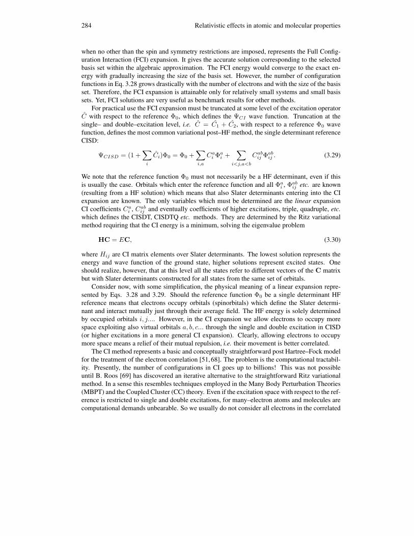
284 Relativistic effects in atomic and molecular properties
when no other than the spin and symmetry restrictions are imposed, represents the Full Config-uration Interaction (FCI) expansion. It gives the accurate solution corresponding to the selectedbasis set within the algebraic approximation. The FCI energy would converge to the exact en-ergy with gradually increasing the size of the basis set. However, the number of configurationfunctions in Eq. 3.28 grows drastically with the number of electrons and with the size of the basisset. Therefore, the FCI expansion is attainable only for relatively small systems and small basissets. Yet, FCI solutions are very useful as benchmark results for other methods.
For practical use the FCI expansion must be truncated at some level of the excitation operatorC with respect to the reference Φ0, which defines the ΨCI wave function. Truncation at thesingle– and double–excitation level, i.e. C = C1 + C2, with respect to a reference Φ0 wavefunction, defines the most common variational post–HF method, the single determinant referenceCISD:
ΨCISD = (1 +∑i
Ci)Φ0 = Φ0 +∑i,a
Cai Φai +∑
i<j,a<b
Cabij Φabij . (3.29)
We note that the reference function Φ0 must not necessarily be a HF determinant, even if thisis usually the case. Orbitals which enter the reference function and all Φai , Φabij etc. are known(resulting from a HF solution) which means that also Slater determinants entering into the CIexpansion are known. The only variables which must be determined are the linear expansionCI coefficients Cai , Cabij and eventually coefficients of higher excitations, triple, quadruple, etc.which defines the CISDT, CISDTQ etc. methods. They are determined by the Ritz variationalmethod requiring that the CI energy is a minimum, solving the eigenvalue problem
HC = EC, (3.30)
where Hij are CI matrix elements over Slater determinants. The lowest solution represents theenergy and wave function of the ground state, higher solutions represent excited states. Oneshould realize, however, that at this level all the states refer to different vectors of the C matrixbut with Slater determinants constructed for all states from the same set of orbitals.
Consider now, with some simplification, the physical meaning of a linear expansion repre-sented by Eqs. 3.28 and 3.29. Should the reference function Φ0 be a single determinant HFreference means that electrons occupy orbitals (spinorbitals) which define the Slater determi-nant and interact mutually just through their average field. The HF energy is solely determinedby occupied orbitals i, j.... However, in the CI expansion we allow electrons to occupy morespace exploiting also virtual orbitals a, b, c... through the single and double excitation in CISD(or higher excitations in a more general CI expansion). Clearly, allowing electrons to occupymore space means a relief of their mutual repulsion, i.e. their movement is better correlated.
The CI method represents a basic and conceptually straightforward post Hartree–Fock modelfor the treatment of the electron correlation [51,68]. The problem is the computational tractabil-ity. Presently, the number of configurations in CI goes up to billions! This was not possibleuntil B. Roos [69] has discovered an iterative alternative to the straightforward Ritz variationalmethod. In a sense this resembles techniques employed in the Many Body Perturbation Theories(MBPT) and the Coupled Cluster (CC) theory. Even if the excitation space with respect to the ref-erence is restricted to single and double excitations, for many–electron atoms and molecules arecomputational demands unbearable. So we usually do not consider all electrons in the correlated

Basic notes on nonrelativistic electronic structure methods 285
treatment. Electrons in lowest–lying orbitals are usually well separated from valence electronsand so they contribute to the atomic and molecular properties very little. In most processes (forexample in reaction or interaction energies) is their contribution cancelled. Therefore, we leavethese so called ”inner shell” electrons uncorrelated. We talk that about these electrons as aboutthe ”frozen core” electrons. Similarly, we do not allow electrons to occupy the highest lyingvirtual orbitals. These computational tricks are well under control since we can verify the inac-curacy caused by omitting inner shell electrons from the correlation treatment. In molecules withatoms as C, N, O, ..., the obvious selection of the frozen core are 1s orbitals. Some caution mustbe payed to so called semi–core–valence correlation. For example, it is insufficient to correlatejust ns2np1 electrons of Ga, In, or Tl. Definitively, also (n-1)d10 shell must be correlated. For,say, the gold atom, we usually correlate valence and core–valence 5p65d106s1 electrons. Specialcaution needs selection of frozen orbitals in relativistic calculations. For Au (and, similarly forPt, Tl, and other atoms) relativistic shifts of orbital energies alters the order of orbital energies,see Fig. 2.3. Also, different components of, e.g., f orbitals, may belong to different symmetries,depending of the symmetry of the molecule. Therefore, we either do not correlate 5s2 and 4fshells or correlate both (which is demanding).
For more accurate solutions of excited states, for simultaneous solving the problem of thedynamical and nondynamical electron correlation, in cases when taking just one determinant isinadequate for representing a reference wave function etc., the Multireference CI (MR CI) isa method of the choice. In this case the reference wave function Φ0 is created as a set of de-terminants, not just as a single determinant. The selection of this wave function is not alwaysstraightforward and needs some experience. Since excitations (again, mostly singles and dou-bles) refer to all determinants in the MR wave function, the MR CI method becomes quicklyintractable with the size of the MR space (so called model space). In general, all determinantswhich are quasi–degenerate must be included. The MR CI method is particularly useful in cal-culations of the bond breaking processes on the hypersurfaces, demanding are problems withconical intersections which may appear in the treatment of reactions in excited states etc. [70].
3.2.5 Coupled Cluster theory
The CI theory discussed in the previous Section was a leading instrument for the high level treat-ment of the electron correlation problem in many–electron atoms and molecules for a long time.Up to the eighties the variational upper bound property, typical for SCF and CI, was consideredas a principal requirement imposed on molecular many–electron methods. For this reason theemerging Many–body Perturbation Theories (MBPT) were considered for the electron correla-tion calculations as less convenient. This view was quite general even though, for example, thefourth order MBPT method was that time appreciated as clearly very accurate and computation-ally much less demanding alternative to CISD [37,62]. Another bottleneck of truncated CI is theproblem of size–consistency, or proper scaling of energy with the size of the system. Size consis-tency means [40] that if the subsystems A and B are far apart, and if energies of A, B, and AB arecomputed in an equivalent way, the computed energies satisfyE(AB) = E(A)+E(B). Relatedto the size consistency is the concept of the size extensivity, which has its analogue in thermody-namics. In many–electron systems was the importance of the size extensivity and the advantagein using an exponential ansatz first realized by nuclear physicists. A quantum mechanical modelis said to be extensive if the energy of a system computed with this model scales correctly with

286 Relativistic effects in atomic and molecular properties
the size of the system. We recommend the reader to study a detailed analysis of these and relatedproblems in the literature, see Refs. [40, 71]. One has to be familiar with consequences of theerrors caused by these effects when calculating intermolecular interactions, reaction energies,bond strength and in many other molecular properties by truncated CI methods, including CISD.Correction can be achieved by including quadruple excitations, at least approximately .
Unlike truncated CI methods, MBPT and Coupled cluster methods provide properly sizeconsistent descriptions. Also, with CC methods higher excitations are considered more effec-tively than in CI methods. Therefore it is worthwhile to pay more attention to CC methodsused frequently also at the relativistic level. Particular attention should be paid to the CCSD(T)method [35, 36] which is presently accepted as a ”golden standard” of quantum chemistry. An-other reason of our attention to the CC theory is that CC methods have been most often usedin our own calculations of molecular properties. The Many Body Perturbation Theory will beshortly discussed in the correlated–relativistic Section 4.5.1.
The Coupled Cluster theory was invented in fifties initially as a tool for understanding corre-lation effects in the electron gas [72–75]. Cızek’s pioneering implementation of the CC theoryto many–electron systems [76–78] represents a real breakthrough in the development of methodsfor the treatment of the electron correlation in atoms and molecules [37–40, 71, 79]. The many–body diagrammatic formulation of MBPT and CC theories as presented in a detailed form byPaldus and Cızek already in 1975 [80, 81] is up to now a wonderful tool for a transparent orderby order analysis of the energy and the wave function. The diagrammatic technique also facili-tates the formulation of final CC equations that obey the requirements of the size consistency andan efficient implementation thanks to clever factorization that alleviates the unpleasant scalingof CC with the number of correlated electrons and the number of virtual orbitals [37, 40, 71, 82].Presently, the CC theory is extremely useful tool for solving a variety of many–body problemsstarting from small systems as atomic nuclei, up to large polyatomic molecules, from weaklybound atoms and molecules up to strongly bound systems as atomic nuclei. Most recent com-prehensive and authoritative account of the CC theory and its applications, including relativistictheory [83, 84] represents a book edited by Carsky, Paldus and Pittner [85].
The essence of the CC theory lies in the exponential expansion of the wave function,
ΨCC = exp(T )Φ0, (3.31)
where T is the excitation operator acting on the known reference state Φ0, which is in most casesrepresented by a single–determinant HF wave function. The excitation operator can be expressedusing the Taylor expansion, so that ΨCC can be written as
ΨCC = (1 + T + T 2/2 + T 3/3! + . . . )Φ0. (3.32)
Expressing the excitation operator T as a sum of all possible excitation operators (up to thenumber of electrons),
T = T1 + T2 + T3 + . . . , (3.33)
leads to different variants of the CC method according to the truncation of the total excitationoperator T at a specific excitation level. Note that upon including all excitation operators the CCwave function and the corresponding energy are accurate within a selected one–electron basis

Basic notes on nonrelativistic electronic structure methods 287
set which defines the reference wave function Φ0. This is equivalent to full CI. The effect of thesingle, double, etc. excitation operators, T1, T2, etc., acting on Φ0 can be expressed in terms ofthe excitation amplitudes tab...ij... defined as
T1Φ0 =∑i
∑a
tai a+i|Φ0〉 =
∑i
∑a
taiΦai
T2Φ0 = (1/4)∑i,j
∑a,b
tabij a+b+j i|Φ0〉 =
∑i>j
∑a>b
tabij Φabij (3.34)
(a+, b+, ..., i, j ...., are creation and annihilation operators, respectively, acting on a Slater de-terminant). More generally, TnΦ0 = 1/(n!)2∑
i,j,k...;a,b,c... tabc...ijk...Φ
abc...ijk.. . Note that in many–
electron theories we prefer to deal with the n–electron reference determinant Φ0 rather thanthe true vacuum state. In the above equations indices i, j, k, ... and a, b, c... etc. refer to occu-pied and virtual spinorbitals in Φ0, respectively, and Φabc...ijk... are determinants representing single,double, etc. excitations from occupied to virtual spinorbitals. General indices will be denoted asp, q, r, s, ....
To get the energy corresponding to the CC wave function |ΨCC〉 defined in the exponentialform, Eq. 3.31, we have to solve the Schrodinger equation,
H exp(T )|Φ0〉 = E exp(T )|Φ0〉. (3.35)
Next, we multiply Eq. 3.35 from left by exp(T ) and obtain:
exp(−T )H exp(T )|Φ0〉 = E|Φ0〉. (3.36)
The Hamiltonian H = exp(−T )H exp(T ) is a similarity transformed Hamiltonian H . It fa-cilitates calculations of nested commutators of the Hamiltonian H with the cluster operator Tneeded for obtaining algebraic expressions for the CC energy and the wave function in termsof one– and two– electron integrals. By projecting Eq. 3.36 onto a reference determinant, |Φ0〉,we obtain the CC energy. The CC excitation amplitudes, tab...ij... and the corresponding CC wavefunction can be obtained by projecting Eq. 3.36 onto all excited determinants, |Φab...ij... 〉:
〈Φ0| exp(−T )H exp(T )|Φ0〉 = ECC (3.37)〈Φab...ij... | exp(−T )H exp(T )|Φ0〉 = 0. (3.38)
At this point it is profitable to employ the Hamiltonian in the normal–ordered second quantizationform as
H =∑pq
fpqp+q+ 14
∑pqrs
〈pq||rs〉p+q+sr+〈Φ0|H|Φ0〉 = fN+WN+〈Φ0|H|Φ0〉. (3.39)
Antisymmetrized two–electron integrals 〈pq||rs〉 are defined in Section 3.2, see Eq. 3.16. Curlybrackets ... denote a normal–ordered string of the second–quantized operators (see, e.g. [40,71, 81]). Subtracting 〈Φ0|H|Φ0〉, the energy of the Hartree–Fock reference state, we have thenormal–ordered form of the Hamiltonian,
HN = fN + WN = H − 〈Φ0|H|Φ0〉. (3.40)

288 Relativistic effects in atomic and molecular properties
Using HN we obtain the CC correlation energy and the wave function,
4ECC = 〈Φ0|HN exp(T )|Φ0〉C (3.41)0 = 〈Φab...ij... |HN exp(T )|Φ0〉C , (3.42)
Eqs. 3.41 and 3.42 may be expressed using the diagrammatic representation of HN and T1,T2, ... Tn, see e.g., Refs. [40, 71, 80, 81]. The subscript C in Eqs. 3.41 and 3.42 indicates thatonly those terms in which the Hamiltonian is connected to the every cluster operator on its rightshould be included in the algebraic representation of the expression. Since HN involves merelyone– and two–electron parts, the expansion of the excitation operator exp(T ) is truncated. Thatmeans, no higher than double excitations, i.e. no higher excitation operators than T1, T2 and theproduct T1T1 (this would correspond to CC with singles and doubles excitations, i.e. CCSD)may appear in any CC energy expression:
4ECC = 〈Φ0|HN (T1 + T2 + 1/2T1T1)|Φ0〉C . (3.43)
The algebraic representation of Eq. 3.43 in spinorbitals is
4ECC =∑ia
fiatai +
14
∑ijab
〈ij||ab〉tabij +12
∑ijab
〈ij||ab〉tai tbj . (3.44)
We stress that above expressions for the CC energy are general. The expression for the CCenergy remains the same when along with T1 and T2 also T3, T4, and so on would be includedin the cluster expansion of T , Eq. 3.33. Of course, the energy itself would be different, since forany truncation of T = T1 + T2 + T3 + . . . different amplitudes enter into Eq. 3.44.
Eqs. 3.42, which determine the tab...ij... excitation amplitudes are truncated by the excitationlevel as well. This time, however, we have to consider which operators are included in theCC exponential expansion, Eq. 3.33. The most common is the CCSD method [86] (CoupledCluster Singles and Doubles), approximating T as T = T1 + T2. This means, that we haveto determine the single and double excitation amplitudes, tai and tabij , respectively. Again, dueto the existence of solely one– and two–electron parts in HN the exponential expansion of theCCSD wave function contains no higher contributions than those from the triple and quadrupleexcitations
|ΨCCSD〉 ⇐=[1 + T1 +
(T2 +
12T 2
1
)+(T1T2 +
16T 3
1
)+(
12T 2
2 +12T2T
21 +
124T 4
1
)]|Φ0〉. (3.45)
By the symbol⇐= we are giving a notice that terms listed in Eq. 3.45 contribute to the CCSDenergy and the wave function. The exponential expansion of the wave function is in fact infiniteand terminates only upon projecting on Φ0, singles and doubles, respectively, see Eqs. 3.41 and3.41. Note that the expansion, Eq. 3.45, contains not only terms easily recognized as single anddouble excitations which arise from the so called connected clusters (terms T1 and T2) but alsotheir products, disconnected clusters T1T1, T1T2, T2T2, up to T 4
1 . T1T2 represents a part ofcontributions due to triple excitations, T2T2 represents a dominating disconnected contribution

Basic notes on nonrelativistic electronic structure methods 289
due to quadruple excitations. For their calculations we need, however, only amplitudes of thesingle and double excitations. This explains the advantage of expressing the wave function asan exponential expansion in CC as compared with the linear expansion in CI (along with thesize–extensivity of CC). The CI coefficients and CC amplitudes can be symbolically related byequations,
C1 = T1
C2 = T2 + (1/2)T1T1
C3 = T3 + T1T2 + (1/6)T1T1T1
C4 = T4 + (1/2)T2T2 + T1T3 + (1/24)T1T1T1T1 (3.46). . .
Theoretical and computational implementation of T3, T4 and even higher excitation operators(which introduce connected contributions of triple and quadruple excitations) is available [82,87–89], but iterative CCSDT, CCSDTQ and higher level methods are prohibitively demanding forother than benchmark calculations of smaller molecules. The algebraic representation of Eq. 3.42is quite complicated even for the CCSD method. The reader is referred to the literature, seee.g., [37, 40, 71, 80]. We just mention that the single and double excitation amplitudes in CCSD,tai and tabij , have to be determined in an iterative process starting from the simplest amplitudes,
which are the first–order wave function tabij amplitudes (tabij(1)). Let us assume that we work with
canonical HF orbitals, for which 〈p|f |q〉 = εpδpq . In the spinorbital form tabij(1) amplitudes are
represented by a simple formula,
tabij(1)
=〈ij||ab〉
εi + εj − εa − εb. (3.47)
The denominator in Eq. 3.47 , (denoted in the following as Dab...ij... )
Dab...ij... = (fii + fjj + . . . )− (faa + fbb + . . . ) = εi + εj + · · · − εa − εb − . . . (3.48)
results from the one–electron part of HN . For the reference determinant with canonical HForbitals, Eq. 3.19, the only nonzero terms are diagonal Fock matrix elements, i.e. orbital energies.We should add that the single excitation amplitudes tai appear for the first time as the second–order terms (however, they are the first order terms for open–shells with the ROHF reference).It is easily recognized that with tabij
(1) defined in Eq. 3.47 we obtain the second order MBPTcorrelation energy (MBPT2),
4E(2)MBPT =
14
∑ijab
〈ij||ab〉tabij(1)
=∑
i<j,a<b
〈ij||ab〉2
εi + εj − εa − εb. (3.49)
The expression is pair additive, that means the correlation energy can be expressed in terms overpairs of occupied (virtual) orbitals. Higher orders of MBPT do not exhibit such additivity. Notethat the expression for4E(2)
MBPT is formally the same as is the second term in the4ECC energy.The only difference is that the amplitudes in 4ECC are the infinite–order tabij CC amplitudes

290 Relativistic effects in atomic and molecular properties
while in4E(2)MBPT there are the first–order double excitation amplitudes (terms with tai are zero
in the MBPT2 energy, since they appear for the first time in the second–order wave function).We will use this simplest nonrelativistic expression for the correlation energy in Section 4.5.1 asa starting point for discussing the theoretical and computational demands when going from thenonrelativistic to the relativistic correlated treatment of atoms and molecules. This instructiveexample may give the reader some idea of what can be expected with higher electron correlationmethods at the four–component relativistic level.
Realizing that all iterative methods lying higher in the hierarchy of the CC methods are com-putationally much more demanding than CCSD, we have to ask a question of including connectedtriples and quadruples in a more approximate way. CCSD contains disconnected contributions oftriples and quadruples, but for accurate results are important connected triples and for quaside-generate systems also connected quadruples. The importance of triples was for the first timedocumented by Paldus, Shavitt and Cızek [78]. The first systematic inclusion of triple excita-tions into the CC theory was studied by Lee, Kucharski and Bartlett [90]. Their approximateiterative CCSDT–1 method was largely extended to a series of the CCSDT–n approximationsof the full CCSDT by Urban et al. [35] based on the careful order–by–order CC wave functionanalysis. Full iterative CCSDT was implemented by Noga and Bartlett [87]. Higher level CCcalculations are also available [40, 91], albeit obtaining an algebraic representation of CC equa-tions beyond CCSDT is extremely tedious. The problem was alleviated by using diagrammatictechniques and the second quantization formalism, leading to the string-based coupled clustertheory and automated generation of computer codes [89], as pioneered by Li and Paldus [92].The critical need for including triples in an economical fashion culminated by introducing thefamous CCSD(T) method. The idea was that the main contributions from triple excitations (4–th order energy terms in the perturbation theory), that are missing in CCSD can be effectivelyadded via perturbation–based technique non–iteratively, using all the ”correlation” informationavailable from the converged T1 and T2 CCSD amplitudes. The CCSD(T) method [35–37], rep-resents perhaps the best compromise between accuracy and efficiency for treating high–levelelectron correlation problem for small and medium size molecules represented by a good singledeterminant reference. As many comparisons with experiment and benchmark FCI and higherlevel CC methods showed, it is accurate enough and still allowing the usage of sufficiently largebasis sets. For its safe use it is recommended checking the suitability of a single determinantreference by inspecting the tai and tabij CCSD amplitudes which should not be larger than 0.20 orto use the diagnostics for single excitation amplitudes (the T1 diagnostics, [71]). We note, how-ever, that even CCSD(T) remains computationally very demanding for large scale calculations.Its importance, besides being an excellent tool for predicting molecular properties lies also in itsrole as a source of benchmark results for DFT methods, which are missing a systematic test ofaccuracy.
In CCSD(T) calculations with large basis sets the most demanding step remains the triplesstep, even though it is noniterative (in contrast to the iterative CCSD). It should be interestingto realize that CCSD(T) for open–shells and for four–component relativistic calculations is evenmore demanding than are nonrelativistic closed–shell calculations. Therefore we will show a fewequations in order to demonstrate the scaling of triples with the number of occupied (No) andvirtual (Nv) spinorbitals.
The CCSD(T) energy is represented by a sum of the converged CCSD energy plus contri-butions from connected triples calculated noniteratively using the perturbative MBPT arguments

Basic notes on nonrelativistic electronic structure methods 291
(for more details see [36, 37, 40, 71]:
ECCSD(T ) = ECCSD + E(CCSD)T + E
(CCSD)ST , (3.50)
where E(CCSD)T is the correction from triple excitations calculated in the fourth order MBPT
fashion,
E(CCSD)T =
∑i<j<k
∑a<b<c
tabcijkDabcijk t
abcijk . (3.51)
Dabcijk is the denominator defined by Eq. 3.48. The triple excitation amplitudes are calculated
using the expression (see, e.g. [37, 40, 71])
Dabcijk t
abcijk = P (i/jk)P (a/bc)
∑d
〈bc||di〉tadjk − P (i/jk)P (a/bc)∑l
〈la||jk〉tbcil . (3.52)
All these equations are presented in the simplest spinorbital form. Eqs. 3.51 and 3.52 look likethe MBPT equations which define the fourth order energy contribution from the triple excita-tion amplitudes. However, triples in CCSD(T) are calculated using the converged CCSD tabij
infinite order amplitudes instead of the first order tabij(1) double excitation amplitudes. P is the
permutation operator. The E(CCSD)T contribution which supplements the 4ECCSD correlation
energy (or ECCSD in a shorter notation) defines the CCSD + T(CCSD) method [35] which is aforerunner of the CCSD(T) method. The difference is that Pople et al. [36] have incorporated inCCSD(T) a single fifth order contribution, E(CCSD)
ST (all other fifth order energy contributionswere neglected), which represents an interaction of singles and triples:
E(CCSD)ST =
∑i,j<k
∑a,b<c
〈bc||jk〉tabcijk tai . (3.53)
The E(CCSD)ST contribution is an analogue of the fifth order contribution to the MBPT energy,
E(5)ST , comprising the single and triple excitations. In CCSD(T) is E(CCSD)
ST calculated, again,employing the converged CCSD tai infinite order single excitation amplitudes instead of the sec-ond order wave function single excitation MBPT amplitudes. Formally the second order MBPTwave function triples amplitudes tabcijk are calculated using Eq. 3.52 from the infinite order CCSDtabij doubles. We note that the tai singles are first order wave function amplitudes for open–shellswith the ROHF (or any other non–HF) reference. For details see [38, 40, 65, 66, 71].
No doubt, the most frequently used CC method, CCSD(T), is computationally much moredemanding than are the SCF or the Density Functional Theory (DFT) calculations. Even moredemanding are CCSDT, CCSDTQ etc. methods and their variants. The role of CC methodsand particularly the CCSD(T) method as a source of benchmark results for e.g., tuning lessdemanding DFT methods can be hardly overestimated. Enormous importance of CC methodslies in their potential for obtaining results with high and controlled accuracy, i.e. good resultsfor a good reason. This follows from the fact that CC methods form a natural perturbative–likehierarchy [35, 37–40, 71] employing gradually more accurate wave functions in more efficient

292 Relativistic effects in atomic and molecular properties
way than in other (for example variational) methods. The efficiency follows from utilizing theexponential ansatz for the wave function, Eq. 3.31. At the same time this ansatz guarantees thesize–extensivity of CC energies [40,71]. We note that an instrument for controlling the accuracyand reliability of frequently used DFT methods is missing. Another problem with DFT is plentyof functionals used in calculations of a specific property and difficulties of DFT in representing,e.g., dispersion forces in Van der Waals interactions, diffuse parts of the electron distributionneeded for proper treatment of electron affinities, etc.
Should CCSD(T) results for smaller molecules serve as a benchmark for other methods,reasonably large basis sets for accurate description of occupied orbitals are required. The numberof occupied orbitals (spinorbitals) is strictly determined by the number of electrons. Large basissets create large space of virtual orbitals and, therefore, enhanced computational demands inthe treatment of the correlated calculations. With the UHF reference the most demanding stepsfor obtaining the single and double excitation amplitudes in CCSD scale with the number ofoccupied (No) and virtual spinorbitals Nv as N2
oN4v in an iterative process. Resulting single
and double excitation CCSD amplitudes are afterwards used in the noniterative approximatedetermination of the triple excitations. Calculations of the triple excitation amplitudes, Eq. 3.52,is the most demanding part in CCSD(T) with large basis sets (for large basis sets is Nv No).The tabcijk amplitudes are carrying three target indices of occupied orbitals and three indices ofvirtuals. Adding the summation over index of the occupied or virtual orbital leads to unfavorablescaling ≈N3
oN4v and N4
oN3v . The final calculation of the energy resulting from triples is slightly
less demanding, scaling as N3oN
3v , see Eqs. 3.51 and 3.53. Worst steps in the rigorous iterative
CCSDT would need arithmetic operations which scale as N3oN
5v in each iteration. Approximate
CCSDT–n methods are a bit simpler but still very demanding. Another problem with CCSDTand CCSDT–n is also storing of N3
oN3v triples amplitudes.
For closed–shell systems the computational cost of CCSD(T) calculations can be reducedby about a factor of 4 when working with orbitals instead of spinorbitals (the number of oc-cupied/virtual orbitals for closed–shells is one half of the number of spinorbitals). Substantialreduction of computer demands for open–shell systems with respect to the UHF reference canbe achieved using the ROHF reference [65]. Theoretical background of the ROHF CCSD(T)method with the spin adapted amplitudes is more complicated [66, 93] than with the UHF ref-erence or methods for the closed–shells with the RHF reference. Theoretical reduction of thecomputer time for closed–shells or for open–shells with the ROHF reference does not corre-spond to the expected factor of reducing the number of orbitals by one half since it is hamperedby more complicated structure of the final equations after applying the spin integration. Clearly,working with four–component spinors makes relativistic CCSD(T) calculations even more de-manding than are nonrelativistic calculations utilizing doubly occupied orbitals for closed–shellsor one–component spinorbitals with the UHF reference.
Modern formulations of the CC theory, sophisticated factorization of complicated equationsfor obtaining CC amplitudes, combined with a quickly enhanced computer power accompaniedwith a high level of parallelism allow calculations of gradually larger and larger molecules witha high and controlled accuracy [64]. Techniques exploited in modern approaches utilize manymathematical ”tricks” and physically well founded approximations like Choleski decompositionfor more efficient treatment of the two–electron integrals (which is a bottleneck in all sophis-ticated many–electron methods), optimization and subsequent reduction of normally very largespace of virtual orbitals (OVOS, Optimized Virtual Orbitals Space), the symmetry constrains

Basic notes on nonrelativistic electronic structure methods 293
etc. [64]. Using of CC methods based on the Douglas–Kroll–Hess Hamiltonian [18, 94, 95], inwhich the scalar–relativistic effects are included needs modified integrals over basis functions(forgetting for a need of modified contractions of basis sets) but otherwise it is quite straightfor-ward. Very efficient are approaches relying on the idea of localized orbitals and also explicitlycorrelated CC methods [96] working with the r12 variables in the wave function. Eventually, CCmethods approach in some cases an almost linear scaling with the size of a molecule, which is adream goal of the quantum chemistry methods for many–electron systems.
Large progress is observed in developments of the Multireference CC methods (MR CC) andapproaches capable of treating quasidegenerate systems [38, 88, 97–99]. MR CC approaches arevery important in relativistic calculations particularly for the SO coupling or QED effects [84].Relativistic CC methods will be discussed in more detail in Section 4.5.2.
3.2.6 CASSCF, RASSCF, and CASPT2 methods
The physical origin of the electron correlation was summarized in Section 3.2.3. We have al-ready introduced a concept of the dynamical and nondynamical correlation. Clearly, both effectscan not be entirely separated and mean just a possible way for understanding a difficult problemof the treatment of inter–electronic interactions in many electron systems. The problem can besomewhat simplified if the starting wave function for high level calculations can be just a singleSlater determinant which is a solution of the HF equations. The single determinant methods fortreating the dynamic correlation were discussed in previous sections. In this part we will summa-rize some methods applicable to problems which require two or more Slater determinants whichrepresent a reasonable starting wave function of a system under consideration. As mentioned inSection 3.2.3 this occurs in investigations of the bond breaking processes, in many open–shellsystems, particularly in low–spin excited states, and other. First indication that the single de-terminant reference is insufficient is a small energy gap between the SCF occupied and virtualorbitals in a single Slater determinant wave function (if used as a reference). In the CISD wavefunction the leading determinant must be strictly dominating (by more than 90%) and the singlyand doubly excitation amplitudes in CCSD must be not larger than 0.2 for calculations with asingle determinant reference. A trivial example of problems with a single determinant referenceis the bond breaking in the hydrogen molecule. It is perfectly well represented by a single deter-minant around the equilibrium bond distances Re. Upon stretching the bond length the potentialenergy curve (calculated within the Born–Oppenheimer approximation) has a reasonable shapeup to distance of about 1.5 Re. For longer distances the energy gap between the bonding σg andthe antibonding σu orbitals gets narrow and the potential energy curve deteriorates. At the fullseparation is the situation simple - dissociation products are just two hydrogen atoms. In mediumdistances, however, we need at least two determinants, corresponding to the electronic config-urations σ2
g and σ2u (having the same spin and the same state symmetry). Analogous orbitals
participate also in the bond breaking in the F2 molecule. More complicated is the situation whenbreaking (or forming) the double or triple bonds in which participate π orbitals. Examples are thedissociation of the ethylene molecule into two methylene radicals or bond breaking of the triple–bonded N2 molecule. The fact that the electronic potential energy curves around minima are formany molecules well represented by energies obtained from the correlated single determinantreference wave functions and methods, like CCSD(T), can be documented numerically: In mostcases the polynomial fit over energies around the minima leads to reasonably accurate harmonic
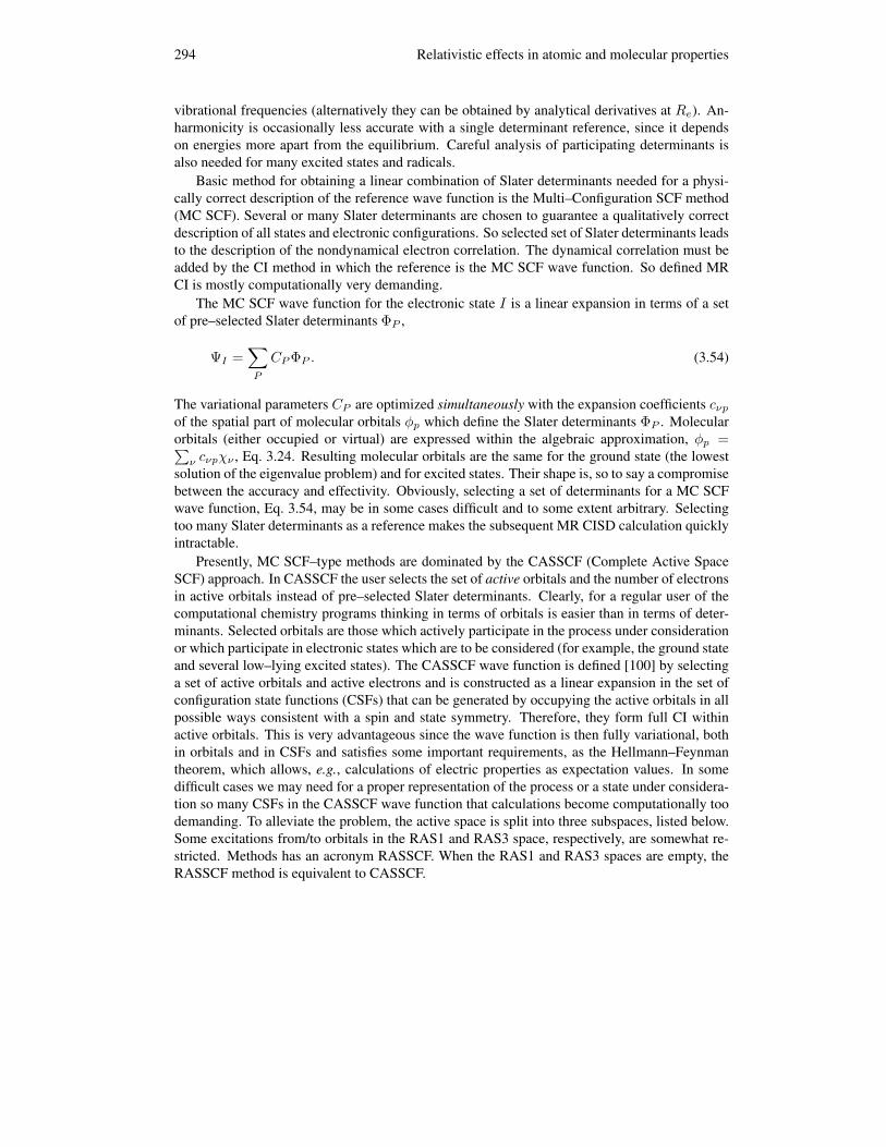
294 Relativistic effects in atomic and molecular properties
vibrational frequencies (alternatively they can be obtained by analytical derivatives at Re). An-harmonicity is occasionally less accurate with a single determinant reference, since it dependson energies more apart from the equilibrium. Careful analysis of participating determinants isalso needed for many excited states and radicals.
Basic method for obtaining a linear combination of Slater determinants needed for a physi-cally correct description of the reference wave function is the Multi–Configuration SCF method(MC SCF). Several or many Slater determinants are chosen to guarantee a qualitatively correctdescription of all states and electronic configurations. So selected set of Slater determinants leadsto the description of the nondynamical electron correlation. The dynamical correlation must beadded by the CI method in which the reference is the MC SCF wave function. So defined MRCI is mostly computationally very demanding.
The MC SCF wave function for the electronic state I is a linear expansion in terms of a setof pre–selected Slater determinants ΦP ,
ΨI =∑P
CPΦP . (3.54)
The variational parameters CP are optimized simultaneously with the expansion coefficients cνpof the spatial part of molecular orbitals φp which define the Slater determinants ΦP . Molecularorbitals (either occupied or virtual) are expressed within the algebraic approximation, φp =∑ν cνpχν , Eq. 3.24. Resulting molecular orbitals are the same for the ground state (the lowest
solution of the eigenvalue problem) and for excited states. Their shape is, so to say a compromisebetween the accuracy and effectivity. Obviously, selecting a set of determinants for a MC SCFwave function, Eq. 3.54, may be in some cases difficult and to some extent arbitrary. Selectingtoo many Slater determinants as a reference makes the subsequent MR CISD calculation quicklyintractable.
Presently, MC SCF–type methods are dominated by the CASSCF (Complete Active SpaceSCF) approach. In CASSCF the user selects the set of active orbitals and the number of electronsin active orbitals instead of pre–selected Slater determinants. Clearly, for a regular user of thecomputational chemistry programs thinking in terms of orbitals is easier than in terms of deter-minants. Selected orbitals are those which actively participate in the process under considerationor which participate in electronic states which are to be considered (for example, the ground stateand several low–lying excited states). The CASSCF wave function is defined [100] by selectinga set of active orbitals and active electrons and is constructed as a linear expansion in the set ofconfiguration state functions (CSFs) that can be generated by occupying the active orbitals in allpossible ways consistent with a spin and state symmetry. Therefore, they form full CI withinactive orbitals. This is very advantageous since the wave function is then fully variational, bothin orbitals and in CSFs and satisfies some important requirements, as the Hellmann–Feynmantheorem, which allows, e.g., calculations of electric properties as expectation values. In somedifficult cases we may need for a proper representation of the process or a state under considera-tion so many CSFs in the CASSCF wave function that calculations become computationally toodemanding. To alleviate the problem, the active space is split into three subspaces, listed below.Some excitations from/to orbitals in the RAS1 and RAS3 space, respectively, are somewhat re-stricted. Methods has an acronym RASSCF. When the RAS1 and RAS3 spaces are empty, theRASSCF method is equivalent to CASSCF.

Basic notes on nonrelativistic electronic structure methods 295
Partitioning of the occupied molecular orbitals in RASSCF and the participation of orbitalsin CASPT2 (which will be defined later in this Section) can be summarized as follows:• Frozen orbitals: Orbitals that are doubly occupied in all configurations in CASSCF and
PT2.• Inactive orbitals: Orbitals that are doubly occupied in all configurations in CASSCF.
Allowed are excitations in the PT2 step.• Active orbitals: These orbitals are subdivided into three separate groups:
– RAS1 orbitals: Orbitals that are doubly occupied except for a maximum number ofholes allowed in this orbital subspace.
– RAS2 orbitals: In these orbitals all possible occupations are allowed (former Com-plete Active Space orbitals).
– RAS3 orbitals: Orbitals that are unoccupied except for a maximum number of elec-trons allowed in this subspace.
• Secondary orbitals: Virtual orbitals that are inactive in CASSCF. Excitations to theseorbitals are allowed in the PT2 step.
The CASSCF method can handle the near–degeneracies very effectively and is particularly suit-able as a starting point for applications to processes on the energy hypersurfaces and in the elec-tronic spectroscopy [100]. The extension of CASSCF to the relativistic domain and particularlyto the spin–orbit interactions will be treated in Section 4.7.2.
The CASSCF wave function is not capable of treating the dynamic correlation effects satis-factorily (unless the active space would be unrealistically large). Therefore, CASSCF is used asa zero–order wave function (a root function) for the multiconfigurational second–order perturba-tion theory, which defines the CASPT2 method [64, 100, 101]. CASPT2 uses orbital excitationoperators applied to the root wave function to express the first–order perturbation function. Withrespect to the structure of the active space we should add that within the PT2 perturbation treat-ment also excitations from inactive orbitals are allowed. They do not participate, however, inoptimization of the CI coefficients in the expansion, Eq. 3.54. The same holds for so calledsecondary orbitals which can be employed in the excitation process in the PT2 step. Finally, aswith CI and CC methods there are frozen orbitals that are not used in any excitation process andremain doubly occupied in both the CASSCF and in the PT2 step. Analogously, some highestlying virtual orbitals are neglected in the PT2 dynamic electron correlation calculations
The problem which had to be solved [100,101] is the definition of the zero–order HamiltonianH0. A good choice in defining the simple enough H0 is a generalization of the zero–order Ham-iltonian based on the HF operator, usual in a single determinant reference perturbation theory.We refer the reader to the original literature [100, 101].
CASSCF, CASPT2, RASPT2 and their generalizations to the relativistic domain, RASSI[102, 103] have been successfully applied to a large variety of problems in chemistry and mo-lecular physics. These methods are implemented into the famous MOLCAS computer pack-age [64]. When the active space is selected properly, the method is sufficiently accurate andreliable. Possible problems may occur due to an inadequate choice of active orbitals [104].Alternative selection/extension of the active space is also a tool for controlling the accuracy.Relativistic treatments include the scalar–relativistic methods based on the Douglas–Kroll–HessHamiltonian [18, 94, 95]. The RASSI method for the treatment of spin–orbit effects will be dis-cussed in Section 4.7.2. Important is also availability of basis sets for both nonrelativistic andrelativistic [105, 106] calculations.
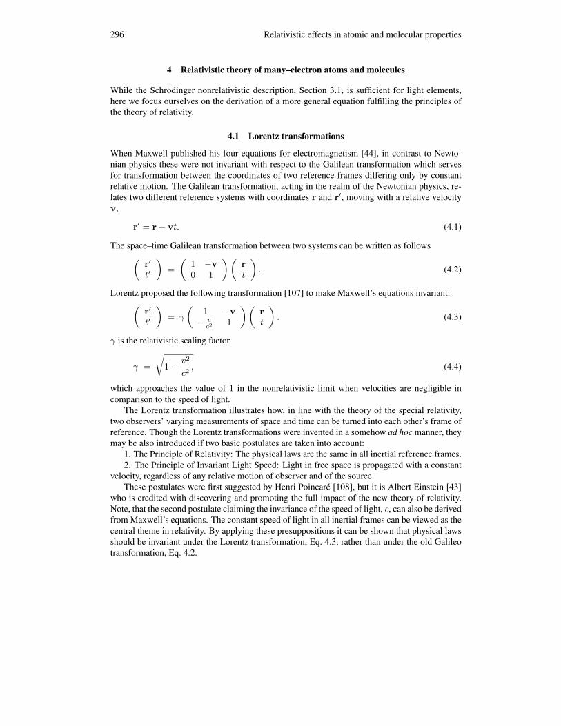
296 Relativistic effects in atomic and molecular properties
4 Relativistic theory of many–electron atoms and molecules
While the Schrodinger nonrelativistic description, Section 3.1, is sufficient for light elements,here we focus ourselves on the derivation of a more general equation fulfilling the principles ofthe theory of relativity.
4.1 Lorentz transformations
When Maxwell published his four equations for electromagnetism [44], in contrast to Newto-nian physics these were not invariant with respect to the Galilean transformation which servesfor transformation between the coordinates of two reference frames differing only by constantrelative motion. The Galilean transformation, acting in the realm of the Newtonian physics, re-lates two different reference systems with coordinates r and r′, moving with a relative velocityv,
r′ = r− vt. (4.1)
The space–time Galilean transformation between two systems can be written as follows(r′
t′
)=(
1 −v0 1
)(rt
). (4.2)
Lorentz proposed the following transformation [107] to make Maxwell’s equations invariant:(r′
t′
)= γ
(1 −v− vc2 1
)(rt
). (4.3)
γ is the relativistic scaling factor
γ =
√1− v2
c2, (4.4)
which approaches the value of 1 in the nonrelativistic limit when velocities are negligible incomparison to the speed of light.
The Lorentz transformation illustrates how, in line with the theory of the special relativity,two observers’ varying measurements of space and time can be turned into each other’s frame ofreference. Though the Lorentz transformations were invented in a somehow ad hoc manner, theymay be also introduced if two basic postulates are taken into account:
1. The Principle of Relativity: The physical laws are the same in all inertial reference frames.2. The Principle of Invariant Light Speed: Light in free space is propagated with a constant
velocity, regardless of any relative motion of observer and of the source.These postulates were first suggested by Henri Poincare [108], but it is Albert Einstein [43]
who is credited with discovering and promoting the full impact of the new theory of relativity.Note, that the second postulate claiming the invariance of the speed of light, c, can also be derivedfrom Maxwell’s equations. The constant speed of light in all inertial frames can be viewed as thecentral theme in relativity. By applying these presuppositions it can be shown that physical lawsshould be invariant under the Lorentz transformation, Eq. 4.3, rather than under the old Galileotransformation, Eq. 4.2.

Relativistic theory of many–electron atoms and molecules 297
4.2 Klein–Gordon equation
The Einstein theory of relativity [43, 109] gives the total energy expression in terms of the mo-mentum and of the rest mass, m0:
E2 = p2c2 +m20c
4; E = ±√p2c2 +m2
0c4. (4.5)
This equation may be utilized to form the classical free particle Hamiltonian, Section 4.3. Thecorresponding quantum mechanical expression is derived by substituting the classical momen-tum, p, by its (three component) quantum mechanical operator, p = −ih∇. The same holds forthe total energy which is replaced by the energy operator, ih ∂
∂t .We insert these operators into the square root of energy expression, Eq. 4.5, and get:
ih∂Ψ(r, t)∂t
= ±c√
(−h2∇2 +m20c
2)Ψ(r, t). (4.6)
The resulting wave equation is known as the Klein–Gordon equation [110,111] and is manifestlyLorentz covariant. However, other aspects of the equation are problematic. It is difficult tointerpret the square root operator. The Taylor expansion is possible, but it would lead to allpowers of the derivative operator and thus to a nonlocal theory. Negative energy solutions havenegative probability densities. Neither does the Klein–Gordon equation handle the spin natureof the electron. These facts lead to rejection of the equation, but in 1934 it found its place as therelativistic wave equation for spin–less charged particles [112].
4.3 Dirac equation
Above mentioned weaknesses motivated Dirac to take the right track and derive a single particleequation overcoming all these problems. Though there were several attempts to formulate thetheory that would couple principles of relativity with those of quantum mechanics, it was Diracwho invented relativistic quantum mechanics for one–electron systems.
Dirac tried to derive an Lorentz invariant equation in the general, time–dependent form (ina.u.)
i∂Ψ∂t
= hDΨ (4.7)
which can be turned, as in the nonrelativistic case (see Section 3.1), into the time–independentform:
hDΨ = EΨ. (4.8)
Eq. 4.7 is linear in the first derivative with respect to time. The Lorentz invariance requires theHamiltonian to be linear in the first derivatives with respect to space as well. Such equation isexpected to have the form (in a.u.)
i∂Ψ∂t
= −ic(αx∂Ψ∂x
+ αy∂Ψ∂y
+ αz∂Ψ∂z
) + βc2Ψ, (4.9)

298 Relativistic effects in atomic and molecular properties
where newly introduced α and β terms must be determined by additional criteria. One of themis that solutions of the new equation must still fulfil the Klein–Gordon equation, Eq. 4.6. PaulDirac commented on the topic: ”It took me quite a while...before I suddenly realized that therewas no need to stick to quantities σ...with just two rows and columns. Why not go to four rowsand columns?” [113]. In this way Dirac found missing terms,
α =[
0 σσ 0
]; β =
[I 00 −I
], (4.10)
with mutual relations
[αp, αq]+ = 2δpq , [αq, β]+ = 0 , α2q = β2 = 1 , (p, q) = (x, y, z), (4.11)
where expression in ”[]+” parenthesis is the anticommutator, [a, b]+ = ab + ba, and δpq is theKronecker delta symbol. σ are 2 × 2 Pauli matrices, mentioned in Section 3.1.2, and I is the2× 2 unit matrix, Eq. 3.10.
Dirac equation posses the form of a 4 × 4 matrix. Further usage of the notation four–component Hamiltonian means the Dirac based energy operator. For the free–electron it canbe written as (in a.u.):
hfeD = cα · p + βc2 =(
c2I cσ · pcσ · p −c2I
). (4.12)
The Dirac relativistic wave function has four degrees of freedom besides the space–timevariable: spin–up (α) and spin–down (β) both for electron and its positively charged conjugatedpartner. It is called the four–component spinor, or shortly four–spinor.
Ψ =(
ΨL
ΨS
)=
ΨLα
ΨLβ
ΨSα
ΨSβ
. (4.13)
The ΨL and ΨS in the Dirac four–spinor are two–component spinors containing large (L) andsmall component functions (S), respectively. The probability density is given as the product offour–component vectors:
Ψ†Ψ = (ΨLα)∗ΨLα + (ΨLβ)∗ΨLβ + (ΨSα)∗ΨSα + (ΨSβ)∗ΨSβ , (4.14)
where Ψ† is a one–row vector:
Ψ† = ((ΨLα)∗, (ΨLβ)∗, (ΨSα)∗, (ΨSβ)∗). (4.15)
The current density vector, j, can be expressed as (in a.u.)
j = cΨ†αΨ. (4.16)
Contrary to the Dirac equation, its nonrelativistic Schrodinger counterpart, Section 3.1, is ofthe second order in momentum. One could say that the Schrodinger equation is suitable for thedescription of a universe where - hypothetically speaking - the speed of light is infinitely high.

Relativistic theory of many–electron atoms and molecules 299
4.3.1 Nonrelativistic limit of the Dirac equation
In general it is important to understand relations between relativistic and nonrelativistic theories.For that reason we establish the connection towards the nonrelativistic limit of the Dirac equation.First, we write the free–particle Dirac equation in the shortened form of two–component spinors:
hfeD
(ΨL
ΨS
)= E
(ΨL
ΨS
). (4.17)
In the next step we express the Dirac equation for the free electron, Eq. 4.12, as a simple set oftwo (2× 2)–dimensional matrix equations (in a.u.):
(c2 − E)ΨL + c(σ · p)ΨS = 0,c(σ · p)ΨL − (c2 + E)ΨS = 0. (4.18)
The small component can be obtained from the second expression of Eq. 4.18
ΨS =c(σ · p)(c2 + E)
ΨL, (4.19)
and inserted it into the first equation:
[(c2 − E) +c2(σ · p)(σ · p)
(c2 + E))]ΨL = 0. (4.20)
We make now the key approximation to approach the nonrelativistic framework: the nonrela-tivistic energy, ε, is positive and very small compared to c2 (in a.u.):
E = c2 + ε ≈ c2. (4.21)
After neglecting the energy contribution ε in the denominator, Eq. 4.20, we get
[−ε+(σ · p)(σ · p)
2]ΨL = 0. (4.22)
Utilizing the identity
(σ · p)(σ · p) = p2, (4.23)
we get a two–component equation for ΨL, which is in fact the Schrodinger equation, Section3.1, for a free electron (in a.u.):
[−ε+p2
2]ΨL = 0. (4.24)
Thus, the large component ΨL can be interpreted as the nonrelativistic limit (c → ∞) of thefour–component solution. Moreover, its two–component solutions
ΨL = cααΨLα + cββΨLβ , (4.25)

300 Relativistic effects in atomic and molecular properties
where α and β are defined in Eq. 3.8, and are carrying information about the spin–orientationof a particle. In this way we have shown that the Dirac equation contains inherently the spinquantum number. This demonstration can also be carried out for a particle in an external field.In the Schrodinger description of the electronic structure the spin quantum number (see Section3.1.2) must be added ad hoc. Note that since the kinetic energy operator, p2/2, is mathematicallyequivalent, according to Eq. 4.23, to (σ · p)2/2, it may be stated that the electron spin is actuallypresent in the nonrelativistic case. Therefore, if the kinetic energy term is present in the form of(σ · p)2/2 in the Schrodinger equation, than the electron spin is involved in the nonrelativisticcase. This would have consequences only in the presence of a magnetic field.
Regarding the small component, Eq. 4.19, by employing the approximation of Eq. 4.21, weget (in a.u.)
ΨS ≈ (σ · p)2c
ΨL. (4.26)
Values of small component, ΨS , are 1c–times smaller (in a.u.) than those of large component,
ΨL.
Negative energy solutions According to Eq. 4.5 solutions for a free particle are symmetricwith respect to zero. They are of continuum type and energies span the range below −mc2 andabove mc2 (or just −c2 and c2 in a.u.). The spectrum is thus not bounded from below and fromabove.
Negative energy solutions worried Dirac: ”One gets over the difficulty on the classical theoryby arbitrarily excluding those solutions that have a negative E. One cannot do this in the quantumtheory, since in general a perturbation will cause transitions from states with E positive to stateswith E negative.” [4].
Negative solutions seemed to be problematic, since it was assumed that a particle has a pos-itive energy. Dirac introduced that the vacuum is the many–body quantum state in which all thenegative–energy electron eigenstates are occupied. Negative states are occupied with particles(i.e. they form the physical vacuum), so that electrons of positive energy do not spontaneouslyfall into negative states with the release of energy. This description of the vacuum as a ”sea”of electrons is called the Dirac sea. Transitions down into the ”Dirac sea” are forbidden bythe Pauli exclusion principle. Any additional electron therefore would be forced to occupy apositive–energy eigenstate. However, there is no need to assume infinite number of particles inthe vacuum since the modern relativistic theory describes both particles and antiparticles in a waythat only the total charge is conserved, but not the total number of all particles and antiparticles.
Dirac stated that if energy higher than 2c2 a.u. is applied on an ”electron” in a negativeenergy state this electron could jump into a positive energy state where it could be observed asan ordinary electron. The remaining ”hole”, i.e. positively charged electron (positron), in thenegative energy state could also be observed. If an electron with positive energy eventually fallsinto this ”hole”, both would disappear with releasing of the energy higher that 2c2 a.u. Dirac’srelativistic theory predicted the existence of the positron, the particle of the weight of an electronbut with the positive charge. This brought a great success for his theory when this particle wasdiscovered in the cosmic radiation by Carl Anderson in 1932 [114].

Relativistic theory of many–electron atoms and molecules 301
Fig. 4.1. Scheme of the Dirac energy spectrum for a free particle (left) and for an electron in the nuclearfield (centre). On the right hand side of the figure there is an energy spectrum with the scale shifted withrespect to the zero energy reference, Eqs. 4.34,4.35.
4.3.2 Solution of the Dirac equation for the hydrogen–like atom
The explicit solution of the Dirac equation for a hydrogen–like atom (in a.u),
hD = βc2 + cα · p + V I, (4.27)
was first published by Darwin [115] in 1928. He honoured Dirac’s outstanding works, Refs.[4, 27], with words ”...one of the great papers in physics in this century”. Excellent modernpresentations can be found in later monographs, for instance Bethe and Salpeter [116], Moss[117], Rose [118] or Messiah [119].
Finding four–component solutions, Eq. 4.13, of the Dirac equation is similar to that for solv-ing the Schrodinger analogue, Section 3.1. Eigenfunctions are written as products of radial andangular terms what leads to the separation into individual angular and radial equations (for com-parison see Eq. 3.3).
The eigenspectrum of the Dirac hydrogen–like operator, Eq. 4.27 (see Fig. 4.1), has threeseparated parts: i) the continuum of negative energy states from −∞ to −mc2 (−c2 in a.u.), ii)another continuum of positive energy states from +mc2 (+c2 in a.u.) to +∞, and iii) a discretespectrum of states between both continuum, leaned towards the bottom of the positive continuum.In the case of the Dirac free particle (Eq. 4.12), the part of the energy spectrum iii) is empty.
Dirac quantum numbers There are four quantum numbers required to specify the state of aDirac hydrogen–like atom. These are similar, but not exactly the same as those of the Schrodinger

302 Relativistic effects in atomic and molecular properties
one–electron atom, Section 3.1, where only three parameters are needed to determine the stateof the electron. The Dirac quantum numbers are:i) The principal quantum number, n, which can have values of 1, 2, 3....ii) The azimuthal quantum number, l, with values of 0, 1, 2, ..., (n−1). This parameter is usuallydenoted by the alphabetical symbols s, p, d, f... However, contrary to the Schrodinger descriptionof the atom, the l number does not represent the orbital angular momentum.iii) The angular quantum number, j. It can carry at most two values, |l± 1/2|. This parameter iswritten as a subscript of the alphabetical symbol of the azimuthal quantum number l.iv) The last parameter is the magnetic quantum number, m, taking all half–odd integer valuesfrom −j to +j.
Regarding pictures of the electron distribution of the Dirac atom, they were published shortlyafter the Dirac’s paper. In 1931 White [120] presented, as continuations to his famous electron–cloud pictures of a nonrelativistic Schrodinger atom, the electron–cloud illustrations of the cor-responding Dirac atom. For more recent pictures of spinors of the Dirac hydrogen–like atom thereader is referred to works like that of Szabo [121].
Shapes of four–component Dirac electronic wave functions are determined by quantum num-bers j and m. Orbitals with identical values of j and m have the same shape, or identical angulardistribution. The s1/2 spinor is spherically symmetrical like the p1/2 one. The pair of d3/2
spinors has the same angular distribution as the pair of p3/2. Furthermore, the p3/2,1/2 (j =3/2,m = 1/2) resembles a ”dog–bone” rather than two touching ellipsoids. Some chemistsfrom the ”old school” might be a little upset to learn that nonrelativistic perpendicular p orbitalsare no longer degenerate and look like a sphere p1/2, a ”doughnut” p3/2,3/2, and a ”dog–bone”p3/2,1/2. All Dirac spinors have electron densities symmetrical about the z–axis and all have aplane of symmetry perpendicular to the z–axis. However, none have nodal planes [121,122]. Themathematical reason for the absence of nodes is due to the fact that all four components of thewave function Ψ (Eq. 4.13) never have nodes all in the same place, because the probability den-sity, Eq. 4.14, is never zero. From a physical point of view this feature is a natural consequenceof the correct handling of the angular dependence for an electron with spin. Schrodinger angulardistributions with nodes are caused by a nonexistent spin–less electron. Likewise no nodes canbe observed already in the simplest case of an electron in a one–dimensional box [116], becausewhenever the large component has a node, the small component remains nonzero. Thus, theanswer to a would–be question of a student - ’How does a p electron pass from one lobe to an-other?’ - is that the physically more general Dirac theory is without nodes. Note, that the correctnodeless results would be obtained already through the Pauli two–component theory. And it iseven possible to construct Schrodinger–type orbitals from certain linear combination of the Diracfour–spinors.
For the determination of nonrelativistic spectroscopic states of chemical systems one needseigenvalues of the angular and spin operators. However, the usual angular momentum operatorof the nonrelativistic theory, Section 3.1.1, does not commute with the Dirac Hamiltonian. It isthe operator, called the total angular momentum for a relativistic particle
j = l +12Σ, (4.28)

Relativistic theory of many–electron atoms and molecules 303
which does. It has the spin–component containing the Pauli matrices, Eq. 3.7, of the form:
Σ =(σ 00 σ
). (4.29)
Components of the operator of Eq. 4.28 satisfy all commutation rules for the angular momentumoperators:
[jp, jq] = ijr, (4.30)
where (p, q, r) labels correspond to cyclic permutations of (x, y, z) components. Analogous tothe relations of the nonrelativistic Hamiltonian, and the angular operators, the square of the totalangular momentum and the z–component of the j–operator commutes with the Dirac Hamilto-nian, Eq. 4.27 :
[hD, jz] = 0 , [hD, j2] = 0. (4.31)
As for the nonrelativistic counterpart, l2, there is a similar eigen equation for the j2:
j2Y4(ϑ, ϕ) = j(j + 1)Y4(ϑ, ϕ), (4.32)
where the eigenfunction Y4(ϑ, ϕ) is the four–component spinor function depending on sphericalangles ϑ and ϕ.
The Dirac equation is rigorous only for a one particle system since it obeys all the require-ments of the special relativity and quantum mechanics. With the hydrogen like atom as the an-alytically solvable model serves as the conceptual background for relativistic theories of many–electron systems.
4.3.3 Finite nucleus
In the nonrelativistic theory the electron–nuclei interaction is usually described by the simpleCoulomb interaction, V = −Zr (in a.u.), where r is the distance of the electron from the pointnucleus with the charge Z. Nonrelativistic orbitals have zero amplitude at the nuclei (centre)except for s–orbitals involving small exponential cusp of the form ∼ exp(−αr).
In relativistic calculations, however, the s1/2 and p1/2 spinors have a weak singularity at thenucleus [123]. Thus it is customary to employ a physically more realistic finite–nucleus modelwhich also improves the basis set convergence [124]. Perhaps the most popular nucleus model isbased on Gaussian distribution, as was proposed by Visser et al. [125]. The nuclear distribution,ρ, and the potential, V , are given by (in a.u.)
ρ = Z(λ
π)
32 exp(−λr2) , V = −Z
rerf(√λr), (4.33)
where erf(x) is the error function. The nuclear exponent λ is chosen in such a way that thenuclear model has the same root–mean–square radius as the experimental value for the nucleus.Recommended values for nuclear parameters were published by Visscher and Dyall [126].
The choice of the nuclear model has negligible effect in cases where only valence spinorsare important for chemical properties. However, there are cases of properties where spinors

304 Relativistic effects in atomic and molecular properties
close to the nuclei are important and the nuclear model may have large influence, and one shouldavoid unphysical point nucleus. Note that the computational implementation of nuclear attractionintegrals is easy as these are only modified two–electron integrals expressed in a Gaussian basisset.
4.4 Four component relativistic quantum chemistry
The relativistic theory of chemical systems appears to be more challenging with respect toestablished nonrelativistic methods based on the Schrodinger equation. Corresponding four–component computational methods are not as good developed as their nonrelativistic counter-parts. The ”reward” for the development of more complex relativistic apparatus is its generality,which fully recovers the nonrelativistic realm in the limit of c→∞, providing in this way the testof the correctness of the implementation. For this reason it is worth to have both nonrelativisticand relativistic energy scales aligned.
The rest energy of the free electron, Eq. 4.21, mc2, is equal to 0.511 MeV. This value, whichis much higher that the binding energy of the hydrogen atom - 13.6 eV, is defined as zero in thenonrelativistic framework. Accordingly, the zero point in the relativistic energy scale is obtainedby subtracting the free electron rest energy. At the operator level this is achieved by subtractingthe diagonal 4× 4 matrix from the β term, Eq. 4.10, and using the modified β′ instead of in theDirac Hamiltonian
β′ =[
0 00 −2I
]. (4.34)
Now we can write the Dirac equation for one electron in a molecular field as[V c (σ · p)
c (σ · p) V − 2c2
] [ψL
ψS
]=[ψL
ψS
]E, (4.35)
where V represents the electrostatic interaction of the electron with the clamped nuclei. Herewe wish to shed more light on the distinction between electron and positron solutions of theDirac equation, as it is not often precisely clarified in the literature. All solutions of the Diracequation, i.e. both of positive and negative energies, are truly electronic because the introductionof potential by the principle of minimal electromagnetic coupling [127] requires specificationof charge [128]. For chemical purposes one sets the charge of the electron e = −1 a.u. andnot the charge of the positron, e = +1 a.u. This assignment was used by Dirac himself [129].The observable positron solutions of the same potential can be obtained by choosing by thecharge conjugation of the negative–energy solutions of the electronic problem, or are calculatedby explicitly choosing the positron charge in the potential.
4.4.1 The relativistic electron–electron interaction
The Dirac equation is valid only for the one–electron system. To extend it for many–electronsystems the proper relativistic electron–electron interaction is to be taken into account. Thestraightforward approach is to augment the one–electron Dirac operator with a two–electroninteraction term. When we consider the Coulomb interaction, what is the simplest case, this term

Relativistic theory of many–electron atoms and molecules 305
is not Lorentz invariant. Although an invariant interaction potential can be derived from quantumelectrodynamics (QED), the fully Lorentz invariant form of the electron–electron interaction termcan not be written in a closed form [123]. Therefore, in practise one prefers truncation to the socalled Breit operator [130],
gBreitij = − 12rij
[αi · αj +
(αi · rij)(αj · rij)r2ij
], (4.36)
which is added to the Coulomb interaction term, 1rij
. The Breit operator accounts for magneticinteractions and retardation effects up to the order of 1
c2 .The first term in brackets on the right–hand side of Eq. 4.36 is the Gaunt interaction term
[131], often used as an approximation of the Breit operator since it includes the largest portion ofthe full Breit form. The Gaunt operator contains spin–spin, orbit–orbit and spin–orbit contribu-tions, while the second term in Eq. 4.36 is the gauge interaction representing retardation effectsinduced by the finite speed of light. Though the Gaunt term itself is not gauge invariant, it is easyto implement within two–electron integral generating codes.
4.4.2 The Dirac–Coulomb–Breit/Gaunt Hamiltonian
The Dirac–Coulomb–Breit/Gaunt (DCB/DCG) operator represents nowadays the most rigorousrepresentation for many–electron relativistic effects. It is formed by selecting the Dirac operatorin a molecular field as the one–electron operator and the Coulomb term, possibly extended bythe Gaunt or the full Breit two–electron term, Eq. 4.36. Keeping the lowest order Coulomb termis the often used approximation of the electron–electron interaction because the two–electronmagnetic interaction terms are typically small.
For the purpose of relativistic quantum chemical calculations one works within the Born–Oppenheimer approximation [54] as in the nonrelativistic framework, Section 3.2. This ap-proximation introduces very small errors in the relativistic quantum mechanical treatment, butcorrections can be applied in the same manner as in the nonrelativistic theory [132].
The aim is to solve the molecular Dirac equation for n electrons localized in the static fieldof N nuclei. The Dirac–Coulomb–Breit/Gaunt Hamiltonian for this general system is
HDCB/DCG =n∑i
hD(i) +12
n∑i 6=j
gBreit/Gauntij +
N∑I<J
ZIZJRIJ
. (4.37)
The one–particle operator, hD(i), is identical with the operator in Eq. 4.35 where the externalpotential is created by static atomic nuclei. Note that the classical potential of the electron in thepoint nuclear field is usually replaced by the finite nuclear distribution, Section 4.3.3.
In comparison to the nonrelativistic many–electron Hamiltonian, Eq. 3.11, it is the one–electron operator that makes the difference which is sometimes accompanied with the gij elec-tron–electron interaction term in its relativistically specified form, see Section 4.4.1.
Brown and Ravenhall problem. A discussion arose about the validity of the DCB/DCG op-erator. The one–electron Dirac equation is not bounded from below and the same holds for the

306 Relativistic effects in atomic and molecular properties
many–electron case. Brown and Ravenhall [133] argued that one can not find stable stationarystates for this Hamiltonian (what is called as the ”Brown–Ravenhall disease”). This is due to thefact that when the electron–electron interaction is treated as a perturbation, one can construct aninfinite number of states for electrons as well as for positrons, causing final states to be com-pletely delocalized. For the case of a two–electron system (like the helium atom) this can bedemonstrated as follows: Let us assume a double excitation from an orbital, where one electronends in the negative energy continuum and the other lands in the positive energy continuum.The sum of their orbital energies is the same (or very close to) as the initial unperturbed energy.Theoretically, when the Coulomb electron–electron interaction is turned on, what would happenis transition to these doubly excited states and subsequent decay of former two–electron boundstate into the continuum. However, the real helium atom does not disintegrate into electrons inthe positive and negative continuum bands. As a remedy Brown and Ravenhall suggested torestrict the Hamiltonian only for positive energy states by applying projection operators. Oncenegative energy (”positron”) solutions are abandoned, the corresponding theory becomes whatis sometimes called as the four–component theory ”for electrons only”, or the no pair approach.However, later it has been found that for practical four–component calculations it is sufficient tohave a proper basis set (see Section 4.4.6) and keep only positive energy solutions [134].
4.4.3 The Dirac–Hartree–Fock method
The relativistic analogue of the Hartree–Fock self-consistent field method (see Section 3.2.1), theDirac–Fock–Breit method, was first formulated by Bertha Swirles [6] in 1935. The story goesthat suggestion came to her by Douglas R. Hartree, who is associated with the Hartree–Focktheory [57, 58], when they were waiting at the London train station [135].
The resulting theory has been implemented first to atoms [7]. Molecular closed–shell for-malism where four–component spinors were used as basis functions were proposed by Malli andOreg [136] in 1975. Later more flexible basis sets were employed for both components coupledby the kinetic balance condition [137–139], see Section 4.4.6.
Both Hartree–Fock and Dirac–Hartree–Fock methods are independent particle models whereeach electron ”feels” the field of nuclei and the average field of other electrons. The derivationof Dirac–Hartree–Fock equations is the same as in the nonrelativistic framework. Shortly, oneseeks the wave function Φ0, which makes the energy functional (for comparison see Eq. 3.18),stationary
EDHF =〈Φ0|HDCB/DCG|Φ0〉
〈Φ0|Φ0〉. (4.38)
The Φ0 wave function is the antisymmetrized product (the Slater determinant, Eq. 3.12) of rel-ativistic one–particle functions, in this case built of four–component spinors, Eq. 4.13. Here wewill label the φ(i) as the four–component spinor representation of the one–electron state. Theexpectation value of the energy can be written as
EDHF =Nocc∑i=1
〈φi|hD|φi〉 +12
Nocc∑i,j
(〈φiφj |gij |φiφj〉 − 〈φiφj |gij |φjφi〉). (4.39)

Relativistic theory of many–electron atoms and molecules 307
The Dirac–Fock operator has the same structure as its nonrelativistic analogue, Eq.3.20:
fDHFφ(i) = (hD + uDHF )φ(i) = εiφ(i), (4.40)
where the Coulomb and exchange operators involved in the uDHF term depend on four–spinors,and are determined in a self–consistent manner.
Since we are seeking electronic states solutions, orthogonal spinors for the Fock operator,Eq. 4.40, must be taken from the positive part of the spectrum. And as we do not allow electronsto enter negative (”positron”) states, the four–component energy operator remains bounded frombelow (also thanks to the kinetic balance condition, see Section 4.4.6), and clear separationbetween negative and positive part of the energy spectrum is retained. The so called Brown–Ravenhall problem, Section 4.4.2, is not relevant for Dirac–Hartree–Fock calculations, althoughthis so called continuum dissolution was a discussed topic in the early eighties.
For the single determinant open–shell system one may employ, for instance, the averageconfigurations formalism [140, 141]. Available is also the four–component multi–configurationSCF version [142, 143], see also Ref. [144].
Solutions of the DHF–equations couple one-electron spin s and orbital l angular momentathrough the j–j or ω–ω coupling. Atomic j–j split shells are as follows: s(2)
1/2, p(2)1/2, p(4)
3/2, d(4)3/2,
d(6)5/2, f (6)
5/2, f (8)7/2 etc., for comparison see Figs. 2.3 and 2.4. Example of molecular ω–ω coupled
shells (σ(2)1/2, π(2)
1/2, π(2)3/2) is given in Fig. 2.5.
Relativistic effects (see Section 2), which are observable already in solutions of the hydrogenDirac equation, Section 4.3.2, are for chemical systems fully manifested within the DHF method.Besides the spin–orbit splitting of l > 0 shells these can be briefly summarized as i) contractionand stabilization of s and p shells which leads to the strengthening of the chemical bond, and ii)relativistic expansion of d and f spinors causing the weakening of the bond.
4.4.4 Symmetry aspects
Computational costs of calculating the energy and properties of any chemical system can begreatly reduced by considering the symmetry of the molecule in question.
Kramers symmetry Since we are in the relativistic domain, the spin–symmetry, Section 3.1.2,can not be used for this type of relativistic operator. Note, however, that by removing spin–orbitinteraction terms from the relativistic Hamiltonian, i.e. keeping the spin–free form, one canemploy the spin–symmetry and single–point group symmetry.
The relativistic replacement of the spin–symmetry is called the time reversal symmetry [119],and is represented by the anti–unitary time–reversal operator which has the form
K = −i( σy 0
0 σy
)K0, (4.41)
where K0 is the complex conjugation operator. The time–reversal operator commutes, in theabsence of the magnetic field, with four–component energy operator, Eqs. 4.37 and 4.40.
Due to the time–reversal symmetry Dirac–Hartree–Fock solutions come out in degeneratepairs, known as Kramers pairs [145,146]. This is the consequence of the Kramers theorem [145]

308 Relativistic effects in atomic and molecular properties
claiming that energy levels of a system with half–integer spin are at least doubly degenerate,and any degeneracy is even–fold. The theorem does not hold in the presence of magnetic field.Relation between two degenerate spinors, representing one–electron states, φ and φ, is
K(aφ) = a∗φ, Kφ = −φ, (4.42)
where a is an arbitrary complex number.
Double–group symmetry In the nonrelativistic theory one deals with point group symmetryoperations acting only on spatial parts of the chemical system. However, with the Dirac Hamilto-nian invariant under symmetry operations, these must be a product of spatial and spin operations,as this four–component operator is coupling both. Therefore, a more general point group com-prising both spatial and spin coordinates has to be introduced. To found the ground for the newgroup theory, rotation by 2π is treated not as an identity operation but as a symmetry operation.Any ordinary rotation group is expanded by taking the product of this new operation. The numberof symmetry operations is thus doubled and these groups are called double groups. Besides theirreducible representations (irreps) used in the nonrelativistic theory, called boson irreps, thereare also irreps that describe one–electron functions of the Dirac–Coulomb Hamiltonian, knownas fermion irreps. The number of fermion irreps is lower than the number of boson irreps. Forexample, a molecule of the D2h symmetry has eight boson irreps but only two two–dimensionalfermion irreps, E1/2g and E1/2u. Likewise the symmetry group of water, C2v , has four differ-ent (one–dimensional) boson irreps, but only one (two–dimensional) fermion irrep, E1/2. Thismeans that fewer two–electron integrals are zero due to the double group symmetry. For thatreason the rigorous four–component symmetry apparatus has to be applied appropriately. Let usconsider a molecule that has only light elements and its energy is computed by using the Dirac–Coulomb Hamiltonian in the double group symmetry. Calculations are much more demandingdue to many two–electron integrals which need to be computed, while most of them are nearlyzero. In this case it is sufficient to resort to one–component quantum chemical methods withadapted single point group symmetry.
The theory for the double group symmetry was first presented by Bethe [147]. There areseveral books [148, 149] of this subject available to the reader, together with many works onthe usage of double groups for constructing relativistic orbitals like Refs. [150–157]. Peng etal. [158] published recently scheme for constructing Kramers paired double group symmetryfunctions.
4.4.5 Classification of relativistic electronic states of atoms and molecules
For atomic systems one takes into consideration also the so called j–j coupling convention as theDirac Hamiltonian commutes with the operator of the total angular momentum, Eq. 4.31. Oneadds the third number, J , representing the size of the total angular momentum, to the spin (S)and angular (L) quantum numbers. For example, the ground state of the thallium atom is X2P1/2,meaning that the valence 6p(1) electron occupies the 6p1/2 (l = 1, s = 1/2, j = 1/2) relativisticspinor. The lowest excited state is 2P3/2 (l = 1, s = 1/2, j = 3/2). Note that the 2P1/2 –2P3/2 spin–orbit interaction splitting serves as a testing ground for a variety of quasirelativisticmethods, see Ref. [159].

Relativistic theory of many–electron atoms and molecules 309
Another case is the lead atom with the valence configuration of 6p(2). While in the spin–freeframework we have X3P, 1D, and 1S states, the spin–orbit coupling gives rise of more states (inascending order): X3P0, 3P1, 3P2, 1D2, and 1S0.
For diatomic molecules one employs the so called ω–ω coupling where the total angularmomentum is
Ω = |Λ + S|. (4.43)
The Ω number is assigned by the group theory as a direct product between the irreducible repre-sentation of the spin and the irreducible representation of the total angular momentum. First, letus have a look at the correspondence between nonrelativistic and relativistic symmetry states. Inthe ω − ω notation the Σ+ irrep is designed as 0+, Σ− as 0−, and Π, ∆, Φ... as 1, 2, 3... TheE1/2 double group representation is labelled as 1
2 , the E3/2 as one 32 in the ω − ω notation. As
an example consider a 3Σ− state of a diatomic. The spatial symmetry (angular momentum) isΣ−, the triplet spin–symmetry (S=1) spans Σ− and Π irreps. The direct product of the spin andspatial symmetries is Σ−(spin) ⊗ Σ−(spatial) = Σ+ and Π(spin) ⊗ Σ−(spatial) = Π. Sothe spin–orbit interaction splits a 3Σ− state into 0+ (Σ+) and 1 (Π) states.
In the 2Π nonrelativistic state the doublet spin corresponds to E1/2 double group representa-tion. Multiplying the spin and spatial irreducible representations, E1/2(spin) ⊗ Π(spatial) =E1/2 + E3/2, gives Ω = 1
2 and 32 electronic states, respectively.
And in the last example, shortly, the 3Π state of some diatomic molecule leads to these ω–ωsplit states (in ascending order): 0+, 0−, 1, 2. The reader can found more in Ref. [160].
4.4.6 Four–component relativistic basis set functions
A common way of solving the molecular Dirac–Fock problem, Section 4.4.3, lies in the expan-sion of molecular spinors in a set of analytic basis set functions. This is ”borrowed” from thenonrelativistic realm where the basis set expansion of the HF–SCF one–electron wave functions,Eq. 3.24, was introduced by Roothaan [63].
In the relativistic domain the one–particle four–spinors are expanded in a separate scalar basisfunctions set for large (L) and for small (S) components:
φp =
φLαpφLβpφSαpφSβp
=
∑i χ
Li cLαip∑
i χLi cLβip∑
i χSi cSαip∑
i χSi cSβip
. (4.44)
The four sets of coefficients, cLα , cLβ, cSα, and cSβ are in general complex. Theupper (L) and lower (S) components of a four–component molecular spinor are expanded as alinear combination of primitive Cartesian Gaussian type of orbitals,
χLi = NLi x
kLi ymLi zo
Li exp(−αLi r2) , χSi = NS
i xkSi ym
Si zo
Si exp(−αSi r2), (4.45)
where N is a normalization constant and k,m, o are parameters whose sum gives the angularmomentum of the atomic orbital.

310 Relativistic effects in atomic and molecular properties
The large χL and small χS component basis functions are related through the so calledkinetic balance condition [137–139]:
χS = − 12c
(σ · p)χL. (4.46)
This condition is nowadays, starting from a given (decontracted) large component set, χL, usedfor constructing the relativistic small component basis set. Note that Eq. 4.46 is derived in thesame way as Eq. 4.26 with employing the shifted energy scale, Eqs. 4.34 and 4.35. In pioneeringyears of the relativistic electronic structure theory the negative energy continuum was sometimesconsidered to be ”guilty” for the failure to get upper bounds of the total energy what was knownas so called ”variational collapse”. However, this was caused by a poor basis set causing badfinite matrix representations of relativistic operators [139]. By employing the balanced basisthe ”unphysical positronic” solutions of the DHF method are easily identified according to theireigenvalues which are about (in absolute value) 2c2 a.u.
Thanks to the basis set expansion, Eq. 4.44, the Dirac–Hartree–Fock problem, Eq. 4.40, canbe reformulated into the matrix representation (analogous with Eq. 3.26)
FDHFC = SCε, (4.47)
which is suitable for an efficient computer implementation. Dyall and coworkers [161–165] arenowadays intensively developing basis sets for all–electron four–component relativistic calcula-tions.
The small component depends on the operator σ · p, acting as a partial derivative with respectto x, y, z coordinates. By applying Eq. 4.46 on large component of Eq. 4.45 with angular momen-tum l one obtains two small component functions with angular momentum l − 1 and l + 1. Thekinetic balance prescription generates the small component basis set which is about two–timesof the size of the corresponding large component basis set. This already indicates that solvinga DHF problem can be quite expensive when compared to the nonrelativistic counterpart. Forthe construction of the two–electron Fock(–Dirac) matrix two–electron atomic integrals (over theCoulomb interaction operator) are sorted into three classes, (LL|LL, (LL|SS), and (SS|SS).Dyall and Fægri stated [25] that in addition to approximately equal number of (LL|LL) inte-grals comparing to the nonrelativistic framework, the number of (LL|SS) integrals is about 13times larger than (LL|LL) integrals and the number of (SS|SS) integrals is approximately 39times larger. The overall computational cost for a DHF calculation in an uncontracted basis setis about 53 times larger than in the corresponding nonrelativistic domain. However, the effect of(SS|SS) integrals is often negligible and their number can be reduced substantially by adoptingsimple Coulombic correction [166]. In the nonrelativistic limit (c→∞) small component basisfunctions, χS , according to Eq. 4.46, disappear and one works with the large component basisset only.
4.5 Relativistic correlation methods
The starting point in four–component relativistic correlation methods is the Dirac–Coulomb–Breit/Gaunt Hamiltonian, Eq. 4.37, in the no–pair approximation, i.e., neglecting positron–electron pair creation. Only electronic states are treated in relativistic correlation calculations.

Relativistic theory of many–electron atoms and molecules 311
By using Kramers unrestricted spinors which correspond to spinorbitals in the nonrelativistictheory, the second quantized form of the Hamiltonian can be expressed by Eq. 3.40. In therelativistic case the fpq are matrix elements over the Fock–Dirac operator, Eq. 4.40. Regardingthe two–electron integrals, the obvious step in correlated calculations is their transformation fromatomic orbital basis to molecular orbitals (spinors) basis. Expression for two–electron integralsin the basis of the four–component Kramers unrestricted spinors, based on the expansion ofEq. 4.44, can be written as
〈φpφq|φrφs〉 =∑X,Y
∑σ,γ
∑i,j,k,l
CXσ∗ip CY γ∗jq CXσkr CY γls 〈χ
Xi χ
Yj |χXk χYl 〉, (4.48)
where X and Y run over large (L) and small (S) components, σ and γ over α and β compo-nents. The φp, φq ... are four–spinors of arbitrary electronic states, either Kramers restricted ornot, coming out of the Dirac–Hartree–Fock procedure, Section 4.4.3, and 〈χXi χYj |χXk χYl 〉 aretwo–electron integrals over (L/S)−atomic basis functions, described by Eq. 4.45. Due to thepresence of atomic basis functions over small component basis functions obtained by Eq. 4.46,the transformation of four–component spinors, Eq. 4.48, is usually computationally most expen-sive part of correlated relativistic calculations. Various speed–ups have been reported, like thatof Abe et al. [167].
4.5.1 Second–order Kramers restricted MP2 method
The simplest and relatively tractable correlation correction to the Hartree–Fock theory is thesecond order Møller–Plesset (MP2) energy [168], given by the general expression for the non-relativistic Hamiltonian
E(2) =14
Nocc∑ij
Nvirt∑ab
|〈ij‖ab〉2|εi + εj − εa − εb
. (4.49)
In connection with four–component relativistic methods we refer the implementation for theKramers restricted closed–shell DHF wave function as was done by Lærdahl et al. [169]. Beingin the relativistic domain, it employs the relation between degenerate Kramers partners, Eq. 4.42,connecting two–electron integrals with ’barred’ and ’unbarred’ spinors:
〈ij‖ab〉∗ = 〈ij‖ab〉, 〈ij‖ab〉∗ = 〈ij‖ab〉,〈ij‖ab〉∗ = 〈ij‖ab〉, 〈ij‖ab〉∗ = 〈ij‖ab〉,〈ij‖ab〉∗ = −〈ij‖ab〉, 〈ij‖ab〉∗ = −〈ij‖ab〉,〈ij‖ab〉∗ = −〈ij‖ab〉, 〈ij‖ab〉∗ = −〈ij‖ab〉.
(4.50)
Inserting these formulas into Eq. 4.49 and carrying out algebraic manipulations we get the sim-plified expression for the Kramers restricted MP2 correlation energy
E(2) =12
No/2∑ij
Nv/2∑ab
1εi + εj − εa − εb
(|〈ij‖ab〉|2 + |〈ij‖ab〉|2 + (4.51)
+|〈ij‖ab〉|2 + |〈ij‖ab〉|2 + |〈ij‖ab〉|2 ++|〈ij‖ab〉|2 + |〈ij‖ab〉|2 + |〈ij‖ab〉|2).

312 Relativistic effects in atomic and molecular properties
The formula Eq. 4.51 is implemented in a direct and parallelized way in the DIRAC [170] pro-gram suite. For that reason an average cost for calculation of the relativistic Kramers restrictedMP2 energy is negligible with respect to the cost of the full four–index transformation, Eq. 4.48,which is necessary for higher level correlation methods, Section 4.5.2, even when employing theKramers restriction.
By replacing the Kramers restricted spinors, Eq. 4.42, with pure spin restricted spinorbitals,Eq. 3.13, one can further reduce the MP2 expression to the form of the nonrelativistic limit. Thisis due to the spin–orthogonality, where densities (pq) = (pαqβ) with an odd numbers of bars(equivalent to β–spin) have no contributions. This leads to the simplified expression
E(2) =12
No/2∑ij
Nv/2∑ab
1εi + εj − εa − εb
(|〈ij‖ab〉|2 + (4.52)
+|〈ij‖ab〉|2 + 2|〈ij|ab〉|2),
and, after the spin–integration we finally get the familiar nonrelativistic expression:
E(2)NR =
12
Nocc/2∑ij
Nvirt/2∑ab
〈ij|ab〉(2〈ij|ab〉 − 〈ij|ba〉)εi + εj − εa − εb
. (4.53)
To compare the effectivity of nonrelativistic and four–component relativistic MP2 calcula-tions one has to take into consideration the transformation over small component basis functionsas the main computational bottleneck, both at the Dirac–Hartree–Fock and the correlated MP2levels, together with higher number of terms in Eq. 4.51 in comparison to Eq. 4.53. The rela-tivistic complete active space second order perturbation theory with the four–component DiracHamiltonian has been reported by Abe et al. [171].
4.5.2 Relativistic Coupled Cluster and Configuration Interaction methods
The Kramers unrestricted Coupled Cluster method with singles, doubles and noniterative con-nected triples CCSD(T), applicable for a wide scale of atomic and molecular systems, was im-plemented by Visscher and coauthors [172]. Authors utilized the spinorbital form of the CCequations (see Section 3.2.5) in the framework of the effectively implemented double–groupsymmetry. Parallelization of the code was carried out by Pernpointer and Visscher [173]. TheKramers restricted CC version was also reported [174], but this program is much less used.
There is another group of relativistic CC methods based on the Fock–space Kramers unre-stricted CC expansion, which give a variety of excited states, see Refs. [175–179].
Relativistic Kramers restricted CI methods are discussed in Refs. [180–183]. Note, that thecomprehensive theory on the generalized Kramers restriction of spinors applicable for open–shellsystems was published by Fleig [184].
4.6 Transformations to two–component Hamiltonians
Four–component Dirac–based theories are connecting ”positron–like” and ”electron–like” de-grees of freedom. In addition, four–component description of the shell structure is always as-sociated with small component basis functions, as mentioned in Section 4.4.6, what increase

Relativistic theory of many–electron atoms and molecules 313
computational time. Without the coupling between the states with negative energy (”positrons”)and the states of positive energy (”electrons”) one would have a possibility to focus on the lat-ter and work solely with the electronic two–component wave function. A high computationalcost of four–component methods is the stimulus towards the development of less demandingtwo–component Hamiltonians dealing with electronic states only, and without the need of small–component basis functions. Methodologies for decoupling charge conjugated degrees of freedomleads to the appearance of a variety of two–component Hamiltonians accurate to various ordersof some expansion parameters.
The following attributes are required for approximate relativistic Hamiltonians: i) Theyshould be accurate enough to give close enough results to corresponding four–component op-erators. ii) They are to be well balanced for treating chemical systems containing a wide varietyof atoms, i.e. both heavy and light. iii) Variational stability together with effectiveness to applythem to moderate and large molecules containing heavy elements.
For two–component methods which include spin–orbit coupling at the orbital level formationthe Kramers restriction and the double–group symmetry, Section 4.4.4, is applicable. Hence onecan utilize the very same (four–)spinors based correlation apparatus, like MP2, Section 4.5.1, CIor CC methods, Section 4.5.2. Let us stress that the main computational saving is due to aban-doning small component basis functions, both at the Hartree–Fock level and at the transformationlevel, Eq. 4.48, what makes them attractive for ’everyday’ relativistic calculations.
Two–component methods can be divided into all–electron and pseudo–potential methods.We focus here on the former group, regarding the latter, we refer the reader to the literature likeRef. [185–189].
In subsequent section we present two known approximate decoupling schemes, the Foldy–Wouthuysen transformation and the Douglas–Kroll transformation. Afterwards we demonstratehow to perform the decoupling transformation up to the infinite order.
4.6.1 Foldy–Wouthuysen transformation
The idea of Foldy and Wouthuysen (FW) [190] was to separate the electronic and positronicsolutions of the Dirac equation by the Van Vleck type unitary decoupling transformation of theDirac Hamiltonian in the form
H ′2comp = UH4compU†. (4.54)
The Foldy-Wouthuysen transformation can be specified in a number of different forms. The mostcommon is the exponential form. Moreover, it can be also expressed as a product of a series ofunitary transformations, U = ...U2U1U0.
For one particle in an external potential Vext and within the single transformation, U =U0 = exp(iS) one gets, after applying the Taylor expansion in the fine structure constant 1/c,the following one–electron terms:
hBP = (mc2 + Vext+p2
2m)− p4
8m3c2+
18m2c2
(p2Vext)+1
4m2c2σ(∇Vext× p)+ ... (4.55)
The definition of S in the exponential above, U0 = exp(βαpp ω(p)
)with a yet unknown pa-
rameter ω(p), as used by Foldy and Wouthuysen [190] in their original work is described in

314 Relativistic effects in atomic and molecular properties
the literature, see Ref. [15, 26]. It is the mandatory starting point for all decoupling schemesemploying unitary transformations of the Dirac Hamiltonian. The first terms in parenthesis inEq. 4.55 represent the usual nonrelativistic Hamiltonian, then the second one is the so calledmass–velocity term, the third is called the Darwin term and the fourth operator describes thespin–orbit interaction. It can be analytically proved that the scalar mass–velocity and Darwinterms are unbounded from below [15]. Carrying out the FW transformation on the entire Dirac–Coulomb–Breit Hamiltonian, Eq. 4.37, one obtains the full two–component Breit–Pauli (BP)operator, which in short notation has the form
HBP =∑i
hBP (i) +∑i<j
gBPij . (4.56)
The transformed electron–electron interaction operator, gBPij contains the Coulomb, spin–orbitand also other interaction terms, like spin–spin and orbit–orbit terms along with numerous highorder terms.
The main disadvantage of the resulting Breit–Pauli Hamiltonian, also known as the first orderrelativistic Hamiltonian, is that its terms are highly singular and variationally unstable. Thereforethis operator is suitable to be used in the first order perturbation theory.
4.6.2 Douglas–Kroll transformation
Douglas and Kroll (DK) pointed out that the FW transformation in an external field yields highlysingular operator which is not suitable for practical calculations. Their approach decouples thelarge and small components of the Dirac four–spinors in the presence of an external potentialthrough successive unitary transformations. The DK transformation is adopting the externalpotential, Vext, as an expansion parameter rather than the speed of light, c, in the FW transfor-mation.
The very first step in the DK transformation is the free–particle FW transformation of theDirac Hamiltonian with the external potential, Eq. 4.27, in the momentum space. Such a termis often referred as the first order DK Hamiltonian, but is unsuitable for practical computations.The DK–proposed operator is of the type
Un = (1 +W 2n)1/2 +Wn, (4.57)
which is unitary if Wn is anti–Hermitian. We shall not go into details of the derivation, butrather give a final form of the DK–transformed operator. The two–component one–electronHamiltonian is then
hDK = Ei+V eff (i) = Ei+Ai(Vext(i)+QiVext(i)Qi)Ai−12
[[Ei,W1(i)]+,W1(i)]+, (4.58)
where [a, b]+ is the anticommutator. Exact form of the Ei, Ai, Qi, W1(i) terms is beyond thescope of the present work and the reader can found them in the literature, like Ref. [15].
Applying the free–electron transformation on a two–electron operator, including the Breitinteraction, Eq. 4.36, we get the two–electron Douglas–Kroll operator:
HDK =∑i
(Ei + V eff (i)) +∑i<j
V effij . (4.59)

Relativistic theory of many–electron atoms and molecules 315
We point to the Dirac relation enabling separation of the spin and spatial operator terms
(σ · a)(σ · b) = a · b + iσ · (a× b), (4.60)
which gives individual spin and scalar (spatial) parts of the Douglas–Kroll transformed operator:
HDK =∑i
(Ei + V sfeff (i) + hDKSO (i)) +∑i 6=j
(V eff−sfij + gDKSO ij), (4.61)
where hDKSO (i) and gDKSO ij are one– and two–electron spin–orbit terms, respectively. For a de-tailed meaning of the terms we refer the reader to the specialized literature, like Ref. [191].
The DK transformation to the second order in the external potential has been extensivelystudied by Hess and coworkers [95, 192]. The third order (DK3) was implemented by Nakajimaand Hirao [193], who applied the DK3 transformation onto the two–electron Coulomb term[194]. Previously Park and Almlof [195] applied only the first order spin–free DK transformationon the Coulomb interaction operator.
In recent years the Douglas–Kroll–Hess (DKH) transformation has been enhanced up tohigher orders. Van Wullen reported the generalized transformation through the sixth order [196].Reiher and Wolf invented a generalized transformation scheme up to the infinite order [197,198].
4.6.3 Exact decoupling
We shall give here alternative derivation of an ’exact’ two–component Hamiltonian and showafterwards its truncation to known approximate forms. First we show equivalence of two ap-proaches for the exact decoupling of negative and positive energy solutions of the DIRAC equa-tion: i) elimination of small components and ii) unitary decoupling transformation.
Similarly as was done for the free particle, Eq. 4.18, we express the Dirac equation for acharged particle in the potential field, Eq. 4.35, as a system of coupled equations for large andsmall components:
h11ΨL + h12ΨS = EΨL
h21ΨL + h22ΨS = EΨS .(4.62)
Let us introduce the operator R representing the exact coupling between small and large compo-nents:
ΨS = RΨL. (4.63)
First we eliminate small components in Eq. 4.62 by using Eq. 4.63. We get
(h11 + h12R)ΨL = EΨL. (4.64)
Than one has to introduce the normalization of individual large–components since these are notnormalized, although enveloping four–component wave functions are normalized to themselves.The normalization operator, N+, can be extracted from normalization condition of the four–component wave function
〈Ψ|Ψ〉 = 〈ΨL|ΨL〉+ 〈ΨS |ΨS〉 = (1 + R†R)〈ΨL|ΨL〉 = 1, (4.65)

316 Relativistic effects in atomic and molecular properties
and is equal to
N+ =√
(1 + R†R). (4.66)
The resulting exact Hamiltonian for the normalized two–component wave function φ = N+ΨL
thereby becomes (the subscript + is representing positive energy solutions,− negative solutions):
h+ = N+
[h11 + h12R
]N−1
+ =√
1 + R†R[h11 + h12R
] 1√1 + R†R
. (4.67)
We are looking for unitary transformation U to decouple solutions of positive and of negativeenergy. The general form (for comparison see also Eq. 4.54 ) comes from Heully et al. [199]:
U†[h11 h12
h21 h22
]U =
[h+ 00 h−
]. (4.68)
Kutzelnigg [200] found the advantage of writing the unitary operator matrix as the product oftwo transformations
U = W1W2 : W 1 =[
1 −R†R 1
]; W2 =
[N−1
+ 00 N−1
−
];
N+ =√
1 + R†R
N− =√
1 + RR†.
(4.69)
The first transformation with W1 leads to the decoupling:[h11 + h12R+ R†h21 + R†h22R −h11R
† + h12 − R†h21R+ R†h22
−Rh11 − Rh12R+ h21 + h22R Rh11R† − R†h12 − h21R
† + h22
]. (4.70)
It is clear for the exact decoupling the off–diagonal elements, which are Hermitian conjugated,have to be equal to zero. This gives relation which is valid only for the exact R:
h21 + h22R = Rh11 + Rh21R. (4.71)
The second transformation W2 introduces the renormalization, thus ensuring the unitarity of thetransformation. In this final step we obtain the Hamiltonian for the positive–energy solutions
h+ =1√
1 + R†R
[h11 + h12R+ R†
(h21 + h22R
)] 1√1 + R†R
, (4.72)
which is identical to Eq. 4.67, when we use the coupling equation, Eq. 4.71.We have shown the equivalence between the elimination of the small components and the
unitary decoupling transformation for the case of the exact coupling between the large and smallcomponents represented by R.

Relativistic theory of many–electron atoms and molecules 317
Regarding the two–component wave functions, we consider the decoupling transformation,Eq. 4.68, of the matrix of four–component eigenvectors,
U†Ψ = W †2 W†1
[ψL+ ψL−ψS+ ψS−
], (4.73)
which gives[ψL+ ψL−ψS+ ψS−
]= W †2
[ψL+ + R†ψS+ ψL− + R†ψS−ψS+ − RψL+ ψS− − RψL−
]. (4.74)
After the exact decoupling small component wave functions for positive energies and large com-ponent wave functions for negative energies are zero, ψS+ = 0 and ψL− = 0. This implies (aftermaking off-diagonal blocks of Eq. 4.74 equal to zero):
ψS+ = RψL+; ψL− = −R†ψS−, (4.75)
One sees that R couples the large and small positive–energy eigenvectors. The final renormalizednonzero two–component functions for separated positive and negative states therefore are :
ψL+ =√
1 + R†R ψL+ ψS− =√
1 + RR† ψS−. (4.76)
The exact coupling between the large and small components of the Dirac equation, Eq. 4.35, canbe expressed as
R =1
2mcB(E) (σ · p) ; B(E) =
[1 +
E − V2mc2
]−1
. (4.77)
This coupling is, however, energy–dependent and thus state–specific. Heully et al. [199] de-veloped a state–universal quadratic equation. The coupling equation obtained in a kineticallybalanced basis set (Eq. 4.46) forms the basis of the iterative XQR scheme proposed by Kutzel-nigg and Liu [201]. The R in Eq. 4.63 will refer to the state universal coupling operator, inagreement with the notation used in the paper by Heully et al. [199]. Finally, one may note thatthe resulting working equation for electronic states,
h+ψL+ = EψL+, (4.78)
can be rearranged to[h11 + h12R+ R†
(h21 + h22R
)]ψL+ = E
(1 + R†R
)ψL+. (4.79)
This corresponds to the Normalized Elimination of Small Components (NESC) [202–204].
Truncation to approximate schemes Several two–component relativistic Hamiltonians canbe obtained using approximate couplings, for which Eq. 4.71 is no longer valid. The previouslymentioned Breit–Pauli Hamiltonian, Eq. 4.55, is extracted using the approximation
R ∼ 12mc
(σ · p) , (4.80)

318 Relativistic effects in atomic and molecular properties
and keeping terms to the order of O(c−2). Difficulties due to the unboundedness and singularityof the Pauli operator are avoided in regular approximations (RA). These are constructed upon theapproximation
R ∼ c
2mc2 − V(σ · p) . (4.81)
The ZORA (Zero–Order Relativistic Approximation) Hamiltonian is obtained from decouplingwith Eq. 4.81 and no renormalization [205–207]. Insertion of the approximate coupling, Eq. 4.81,into the NESC equation, Eq. 4.79, gives the IORA (Infinite Order Regular Approximation) equa-tion [208]. A precursor to IORA was the scaled ZORA approach [209], which is an approxi-mation to IORA obtained by replacing the operator product R†R in Eq. 4.79 by its expectationvalue. Comparing the exact coupling, Eq. 4.77, with the regular approximation, Eq. 4.81, onesees that the latter is obtained from the former simply by setting the energy to zero. Note thatmost recently ZORA was implemented in a new relativistic treatment in the Quantum MonteCarlo technique [210].
There is another decoupling strategy: performing first the free–particle Foldy–Wouthuysentransformation [190] which gives a two–component kinetic energy operator on square root formwhat ensures the variational stability of the resulting operator. Subsequent decoupling in ordersof the external potential V (or in the inverse speed of light in c−1) defines the previously men-tioned Douglas–Kroll–Hess [94, 95, 192], Section 4.6.2, and Barysz–Sadlej–Snijders [211–216]transformations, respectively. Alternatively, the small components may be eliminated and theexact coupling obtained through iterative procedures [217–219].
4.6.4 Infinite order two–component Hamiltonian (IOTC)
One may obtain the exact coupling [211,213,214,216] in the finite basis approximation by solv-ing the Dirac equation, Eq. 4.35, in some suitable basis set. The exact decoupling can be carriedout in a single step starting from a matrix representation of the Dirac operator in a molecularfield.
The coupling relations, Eq. 4.75, are in a finite basis set transformed into two systems oflinear equations
Y S+ = RY L+ ; Y L− = −R†Y S− , (4.82)
where Y L(S)+(−) is the block of the eigenvector matrix corresponding to the large (small) compo-
nents of the positive (negative) energy solutions of the Dirac equation. The coupling operator R,Eqs. 4.63, 4.77, now in a matrix form (without the ”hat” symbol), can be obtained directly bysolving the first of system of equations, but in practice it turns out to be better to take the Hermiteconjugate of the second system and premultiply it by Y S− giving
AR = B; A =[Y S− Y
S†−
]; B = −
[Y S− Y
L†−
]. (4.83)
The A matrix is positive–definite and Hermitian. The system can accordingly be solved bya Choleski decomposition. The unitary transformation can now be constructed and the DiracHamiltonian decoupled in matrix form.

Relativistic theory of many–electron atoms and molecules 319
Another important point is that in a rigorous construction of a two–component relativisticHamiltonian the decoupling transformation should be defined with respect to the complete elec-tronic Hamiltonian, Eq. 4.37, not only to the one–electron part, as is usually done in the literature.Evidently, not only the one–electron part, but the two–electron part as well should be subject tothe change of picture transformation. However, this would bring the computational cost backto the four–component level [194, 195]. Therefore, in the two–component electronic Hamilto-nian one prefers untransformed two–electron Coulomb term, which implies that two–electronspin–orbit contributions (see Section 4.7) are neglected.
Calculation of properties. Change of picture. Till now various transformations to the two–component form have been demonstrated solely on the Dirac energy operator. In the relativis-tic quantum mechanics, however, one works with a variety of four–component property opera-tors. For this reason, to be physically fully consistent at the two–component level, all relativisticproperty operators have to undergo the very same transformation as the ’parental’ Dirac Ham-iltonian. Clearly, when ’descending’ to the two–component framework, one has to adapt anyfour–component operator accordingly. The adaptation of the operator with respect to the wavefunction is known as the change of picture [220, 221].
For the IOTC case the picture change transformation matrix U , Eq. 4.69, can be appliednot only for the Dirac operator, but also for any four–component property operators in matrixrepresentation as well. Thus the picture change transformation of a four–component propertyoperator in the basis set, X4c, can be done easily:
U†X4cU → X2c++ . (4.84)
It should be stressed, however, that the decoupling transformation U is constructed to block–diagonalize a specific one–electron Hamiltonian, defined by the external scalar potential V ap-pearing in Eq. 4.35. Hence, in general, the decoupling transformation does not block–diagonalizean arbitrary operator. Therefore, elements of the two–component operator,X2c
++, are obtained byselecting the (++)–matrix block, see Eq. 4.73, of the transformed operator. This corresponds toprojecting the four–component operator onto the space spanned by the positive–energy solutionsof the particular Hamiltonian defining the decoupling transformation. At the algebraic IOTClevel the importance of the change of picture for expectation values was reported by Kedzieraet al. [222]. Note that relativistic picture change transformations of the two–electron interactionterm have been reported in Refs. [194, 195, 223].
Implementation of the IOTC method The implementation was described by one of us (MI)[224] and is distributed within the DIRAC08 program suite [170].
The Dirac equation, Eq. 4.35, is solved in the orthonormal (MO) basis [225] and subsequentlythe IOTC Hamiltonian with positive energy solutions only is then projected back onto the largecomponent AO–basis. This algorithm runs as follows:
1. Setting up the Dirac equation on matrix form in the AO–basis
hAOcAOi = SAOcAOi εi; SAO =[SLL 0
0 SSS
], (4.85)

320 Relativistic effects in atomic and molecular properties
where SAO is the overlap matrix. Uncontracted Gaussian basis functions are used in theimplementation.
2. Transforming to an orthonormal basis using the non–unitary transformation
hMOcMOi = cMO
i εi; V =[V LL 0
0 V SS
];V †SAOV = I. (4.86)
In our implementation the so called restricted kinetic balance (RKB) is enforced in thisstep by embedding the transformation to Dyall’s modified Dirac equation [225,226] in thetransformation V , as described in Refs. [128, 225].
3. The eigenvalue problem, Eq. 4.86, is solved by the diagonalization and the coupling matrixR is extracted using Eq. 4.83. The transformation matrix U , Eq. 4.69, is constructed, andsubsequently the positive–energy two–component relativistic Hamiltonian hMO
+ , Eq. 4.72,is obtained in the matrix form.
4. In the final step the Hamiltonian is projected back onto the large component AO–basis
hAO+ =[V LL;†]−1
hMO+
[V LL
]−1;[V LL
]−1= V LL;†SLL;AO. (4.87)
The matrix representation of the IOTC Hamiltonian, hAO+ , is then written to file with what-ever transformed property operators are needed and all the subsequent calculations con-tinue in the two–component framework.
In comparison to the scheme proposed by Jensen and Ilias [227] the preliminary free–particleFW transformation is completely avoided. Since this transformation was used by Barysz andcoworkers [211–214], we will refer to the two–step approach as BSS. The direct constructionof the coupling matrix emphasised here was already proposed by Dyall [204] as well as Kutzel-nigg and Liu [201, 228], although the latter authors seem to prefer an iterative approach. Thenoniterative algebraic approach to the IOTC relativistic theory was published by Kedziera andBarysz [229]. In the same group it has been shown recently how to recover four–componentsolutions by the inverse transformation of the IOTC wave function [230].
Tab. 4.1 displays ionization energies and electron affinities of the radon atom computed withthe Fock–space Coupled–Cluster method, see Section 4.5.2. We utilized four–component DC,and two–component BSS and IOTC Hamiltonians, all of them including both scalar and spin–orbit effects. The IOTC and BSS Hamiltonians give results closely matching the DC data.
Tab. 4.2 shows NMR shielding constants (see also Section 5.7), magnetizabilities and polar-izabilities of the Rn atom calculated with the DC, IOTC and BSS Hamiltonians. These proper-ties were obtained upon the DC/IOTC/BSS Hartree–Fock wave function with the second orderlinear–response module [232]. Two–component IOTC and BSS results agree with each other andfollow the corresponding four–component DC values.
4.7 Spin–orbit effects
The four–component Dirac Hamiltonian contains by default both scalar and spin–orbit effects.Note that its modification is possible in order to distinguish between those relativistic effects

Relativistic theory of many–electron atoms and molecules 321
according to K. Dyall [226]. Dyall’s adaptation of the Dirac Hamiltonian was enhanced byadopting the so called quaternion symmetry by Visscher and Saue [225]. Although leaving outspin–orbit effects creates some computational speed up in the four–component framework dueto the use of the single point group symmetry, small component basis set functions still remainand cause a computational bottleneck.
Therefore a better way is transforming the four–component Hamiltonian to a two–componentform, Section 4.6, and afterwards separate spin–orbit terms according to Eq. 4.60. Here we givethree examples of SO Hamiltonians. Note that in following formulas for spin–orbit operators weprefer to use Pauli matrices (see Section 3.1.2) instead of spin operators, utilized in Eq. 2.11.
i) Applying the FW transformation on the DCB Hamiltonian, Section 4.6.1, one can extract(from Eq. 4.56) the full spin–orbit Breit–Pauli Hamiltonian [53] of the form
HBPSO =
e2h
4m2c2
(∑i
∑I
ZIriI × pir3iI
· σi −∑i 6=j
rij × pir3ij
· (σi + 2σj)). (4.88)
Tab. 4.1. Ionization energies (IE) of the Rn atom and excitation energies (EE) of the Rn+ cation calculatedby the Fock–space CCSD method [in eV]. Absolute differences from DC values in parentheses. Data fromRef. [224].
DC IOTC BSS
IE of Rna1S0 – 2P3/2 10.5614 10.5304 10.5304
(-0.0310) (-0.0310)EE of Rn+
2P3/2 – 2P1/2 3.7706 3.8967 3.8953(0.1261) (0.1247)
2P3/2 – 2S1/2 14.8708 14.8427 14.8420(-0.0281) (-0.0288)
a Experimental value of the first IE (1S0−2P3/2) is 10.7485 eV, Ref. [231].
Tab. 4.2. Magnetic and electric properties of the Rn atom. Absolute differences from DC values are inparentheses. Data from Ref. [224].
Property DC IOTC BSS
NMR shieldinga 23348.4 23373.6 (25.2) 23372.4 (24.0)Magnetizabilityb -12.7160 -12.7230 (-0.0070) -12.7236 (-0.0076)Polarizabilityc 27.066 27.119 (0.053) 27.122 (0.056)
a NMR shielding constants in ppm.b Magnetizabilities in a.u.c Polarizabilities in a.u.

322 Relativistic effects in atomic and molecular properties
ii) Through the Douglas–Kroll–Hess (DKH) transformation, Section 4.6.2, one may separate (byadopting Eq. 4.61) the variationally stable spin–orbit Hamiltonian
HDKSO = e2h
(∑i
∑I
BiZIr3iI
σi · (ri × pi)Bi −∑i6=j
(BiAjrij × pir3ij
· σiBiAj
+2BiAjrij × pir3ij
· σjBjAi)). (4.89)
The Douglas–Kroll SO Hamiltonian, Eq. 4.89, contains projector operators and the Breit–Paulispin–orbit Hamiltonian, Eq. 4.88, can be obtained by expanding and truncating the kinematicfactors Ai and Bi in both one– and two–electron operators, see, e.g., Ref. [15]. Note that thetwo–electron SO terms appearing in Eqs. 4.88,4.89 are known as the spin–same–orbit (SSO)and spin–other–orbit (SOO) terms, respectively. Both of them are an approximation of the fullCoulomb–Breit/Gaunt interaction operator, see Section 4.4.1.
iii) Since it is difficult to compute different types of two–electron spin–orbit integrals, asa cheap alternative one can utilize an effective one–electron spin–orbit operator of the generalform:
HeffSO =
e2h
4m2c2
∑i
∑I
ZeffI
riI × pir3iI
· σi, (4.90)
where Zeff is a parameter. However, since the two–electron contribution does not scale as theone–electron spin–orbit term, this SO–operator is state dependent and therefore less accurate.
4.7.1 Mean–field spin–orbit operator
Calculation of many–centre two–electron spin–orbit integrals is costly [159, 191, 233] and isapproximately equal to the cost of two–electron integrals over small–component basis functions,Section 4.4.6. This disadvantage has been overcome by introducing a pseudo one–electron Focktype spin–orbit operator, called as the mean–field spin–orbit operator, MFSO. It is an effectiveone–centre operator obtained from the full DKH atomic spin–orbit Hamiltonian [234], Eq. 4.89.
Atomic matrix elements of the MFSO operator have the form:
〈i|hMFSO|j〉c = 〈i|hDKSO (1)|j〉c + 12
∑mf−orbsM nM (2〈iM |gDKSO (1, 2)|jM〉c−
〈iM |gDKSO (1, 2)|Mj〉c − 〈Mi|gDKSO (1, 2)|jM〉c) , c = (x, y, z),(4.91)
where one– and two–electron spin–orbit terms are given in Eq. 4.61. The two–electron part of thisoperator is represented as the summation running over occupied (mean–field) spatial M(l,ml)atomic orbitals; nM are occupation numbers. The orbitals M can be taken either from contrac-tions of the basis set, or, what was preferred here, from an interfaced internal atomic SCF codeproducing scalar relativistic orbitals for a given set of orbital exponents.
A two–component Hamiltonian accounting for both scalar and spin–orbit relativistic effectscan be simply constructed by combining available operators. In the previous work [235] wehave employed the no–pair Hamiltonian containing the one–electron spin–free Douglas–Kroll–Hess term, DKH2sf, which is accurate to the second order in the external potential, together

Relativistic theory of many–electron atoms and molecules 323
with the MFSO operator, Eq. 4.91. Note that from Section 5 onward the acronym DKH is usedsolely for the DKH2sf operator. The two–electron interaction was represented by the standardnonrelativistic Coulomb interaction term.
HDKH2sf+MFSO =∑i
(hDKH2sf (i) + hMFSO(i)) +∑i<j
1rij. (4.92)
The mean–field spin–orbit operator can be expressed as:
hMFSO = hMFSO(x)σx + hMFSO(y)σy + hMFSO(z)σz. (4.93)
The spin–orbit term in the Hamiltonian is the reason why one can not utilize the spin symme-try and work with spinorbitals. One has to resort to general two–component spinors, ΨL ofEq. 4.13. The platform for the implementation was another four–component relativistic programsuite, MOLFDIR [236], which fully utilizes the relativistic double–group symmetry, Section4.4.4. MOLFDIR performs Kramers restricted four– and two–component single determinantHF–SCF calculation on closed– or open–shell system (see Section 4.4.3), followed by electroncorrelation methods, Section 4.5. MOLFDIR was slightly modified in such a way that its two–component mode handles external one–electron integrals of the hDKH2sf and hMFSO operators.
The effectiveness of this operator was demonstrated on FO and ClO molecules in Tabs. 4.3and 4.4. For these light systems DKH2sf+MFSO results follow closely four–component DCGcounterparts. However, for treating heavier elements one has to resort to the Hamiltonian infinitein both scalar and spin–orbit terms, Section 4.6.3.
Tab. 4.3. Spin-orbit splitting of the 2Π state of the FO molecule [cm−1]. Calculated in decontracted basissets, 1s spinors of fluorine and 1s spinors of oxygen were frozen. Data from Ref. [235].
Method/Hamiltonian DKH2sf+MFSO DCG
SCF 183.5 184.9CCSD(T) 194.1 194.4Experiment 193.81
Tab. 4.4. Spin–orbit splitting of the 2Π ground state of the ClO molecule [cm−1]. Calculated in decontractedbasis sets, two sets of spinors, 1s spinors of oxygen and 1s, 2s, 2p spinors of chlorine were frozen. Datafrom Ref. [235].
Method/Hamiltonian DKH2sf+MFSO DCG
SCF 223.3 225.2CCSD(T) 310.7 312.6Experiment 318

324 Relativistic effects in atomic and molecular properties
4.7.2 RASSI–SO
The so called RASSI–SO [102] method belongs to the group where spin–orbit relativistic effectsare treated a posteriori in the so called L–S or Russell–Saunders coupling scheme [237], see alsoRef. [233], which is based on the combination of many–electron states with the resultant angularand spin momentum numbers, L and S, respectively, leading to a new wave function of a totalangular number J . The spin–orbit interaction in accounted for through a multiconfigurationalinteraction approach, which employs the Complete Active Space (CASSCF) or Restricted ActiveSpace (RASSCF) wave functions as a reference.
Relativistic effects are treated in two steps as follows: First, the CASSCF/RASSCF wavefunction is calculated for a specified total spin S, and can be viewed as a common represen-tative of all possible spin states within the given multiplet. Its advantage is that this spin–freebasis can involve many wave functions, and these may use individually optimized molecular or-bitals. Such determined scalar relativistic wave functions include both static (through the use ofthe multideterminantal RASSCF/CASSCF method) and dynamic correlation effects (using themulticonfigurational perturbation theory, CASPT2).
In the second step, one computes eigenstates of a two–component quasirelativistic Ham-iltonian in a basis set of spin–free (scalar) wave functions. The matrix over spin–free states,where the Hamiltonian operator contains the Douglas–Kroll–Hess scalar term together with theAMFI operator, Eq. 4.91, is calculated by an extension of the Restricted Active Space Interaction(RASSI) method, and is utilizing the Wigner–Eckart theorem due to the spin–orbit operator.
To include the dynamic correlation within, one can employ the multi state (MS) CASPT2method in the RASSI–SO procedure for calculation of spin–orbit matrix elements. The MS–CASPT2 method is mixing CASSCF states and the resulting SOC wave functions are mixturesof CASSCF functions of different space and spin symmetry.
Matrix elements over the original basis as well as over the eigenstates can involve also otherproperty operators, and can be used to calculate, for example, transition strengths.
4.8 Fine effects, Lamb shift
Although the Dirac theory predicts the entire spectrum of the hydrogen–like atom, some cases ofthe fine splitting are not covered. Lamb and Retheford [238] discovered (1947) in a microwaveexperiment that the 2s1/2 level was higher than the 2p1/2 level by 1.060 MHz. According to theDirac theory, both states, 2S1/2 and 2P1/2 should have equal energy. Bethe [239] was the firstto explain the very small shift, called the Lamb shift, in the hydrogen spectrum. This was thebeginning of modern Quantum Electrodynamics, QED.
Dirac’s theory does not deal with the possibility of creating and destroying particles, whichis one of the basic consequences of the theory of relativity. An extension using the quantizedelectromagnetic field leads to the theory of quantum electrodynamics, which fixes this difficulty.According to the QED theory electrons and positrons appear as quanta of the quantized Diracfield. Vacuum fluctuations are perceived as zero point oscillations of this field. The interactionof an electron with zero–point oscillations of the electromagnetic field creates its self–energy,which is, together with effect of vacuum polarization, observed experimentally. The self–energyis the largest QED correction reducing the binding energy of an electron due to the exchangeof virtual photons with the nucleus. The vacuum polarization contribution causes shift in the
Relativistic theory of many–electron atoms and molecules 325
binding energy of an electron due to the creation and annihilation of virtual e−–e+ pairs in thevacuum. It increases the binding energy mostly of the time and is the second largest correction.In the two excellent reviews published recently by Lindgren, Salomonson a Hedendahl [83] andEliav and Kaldor [84] discussed physical aspects of QED effects in physics and chemistry andpresent computational tools for incorporating of QED within the Coupled Cluster formalism forelectron correlation effects.
The value of the Lamb shift scales as the fourth power with respect to the nuclear charge Z,thus is rather important for heavy systems. For instance, a good example is the U91+ cation,where the shift is of the order of 105 cm−1, what was confirmed experimentally [240].
It appears that QED corrections may be chemically important in the electron binding energyof the eka–radon (Z=118) amounting to a 9% reduction of this property [241]. Eka–radon is asuperheavy element for which a relatively large QED effect is not so much surprising. However,in compounds with rather light atoms as BF3, AlF3, and GaF3 it appears that the Lamb shift tothe atomization energies may be in the range of 3–5% of the scalar relativistic contribution [242]and may be important for higher accuracy calculations particularly for molecules containingheavy elements. Hirao et al. [243] calculated ionization energies of Zn and Mo12+ and concludethat unprecedented accuracy can be achieved by using the fully relativistic many–body treatmentincluding the Lamb shift.
When working in relativistic molecular calculations with the no pair approximation (i.e. oneworks with electronic states only), all QED effects are thus neglected.

326 Relativistic effects in atomic and molecular properties
5 Relativistic effects in atoms and molecules, their properties and interactions
Accurate calculations of atomic and molecular properties require sophisticated many–electrontheories for treatment of the electron correlation problem. This is computationally very demand-ing even at the nonrelativistic level for medium or larger molecules. In so called wave functionmethods the starting point is the HF wave function expressed most frequently in the form of theSlater determinant, Eq. 3.12, as a reference. A single–determinant HF reference wave functionis usually sufficient for closed–shell atoms and molecules. For high–spin open–shell systems thesimplest reference is the single–determinant ROHF wave function. In quasidegenerate situationsthe reference is a combination of Slater determinants. Many problems require a reference con-sisting of more than a single–determinant reference. This is the case of quasidegenerate systems,like calculations on the hypersurface far from the equilibrium geometry or many excited states.A multideterminant reference is also needed for treatment of the SO coupling.
Let us remind (see Section 3.2.5) that at the simplest single–determinant level most demand-ing steps in sophisticated many–electron methods, like CCSD, scale with the number of occupied(No) and virtual orbitals Nv as N2
oN4v in an iterative process. Number of operations required for
triples scales as N3oN
4v . When using the spinorbital basis for open–shell systems with the UHF
(Unrestricted Hartree Fock) reference, we have to treat twice as much spinorbitals when com-pared to the number of closed–shell or ROHF open–shell orbitals. The number of operationsfurther increases for calculations in which we work with 4–spinors (see Section 4). In spite of anenormous progress in technology of CC calculations (see, e.g., our implementation of CCSD(T)in the MOLCAS program [64]), they still remain computationally demanding, particularly, whencombined with specific requirements on the construction of basis sets with some relativistic Ham-iltonian. This explains that rigorous computational applications of ideas of the relativistic theoryfor many–electron atoms and molecules is much more complicated than it is in the nonrelativisticcase.
Orbitals or spinorbitals in the Slater determinant, Eq. 3.12, are in practical nonrelativisticcalculations expressed in the form of the linear combination of atomic basis functions, mostlycontracted Gaussians, [39, 51, 62, 244]. Selection of basis sets for practitioners of relativisticmany–electron calculations is rather delicate. In Section 4.4.6 we learned that there are specificrequirements on basis sets which are capable of representing the large and small components ofthe Dirac spinors. Nonrelativistic basis sets are not applicable for such calculations. A smallcomponent set of exponents is obtained from the large component set and leads to basis setswhich are too large for practical use. Also, in most calculations of atomic and molecular proper-ties we need just a large component. The remedy is the Foldy–Wouthuysen transformation to atwo–component Hamiltonian. Theoretical background of these methods is described in Section4.6. Most frequently used relativistic calculations employ no–pair DKH methods which provideexcellent results in situations when the spin–orbit coupling can be safely avoided. Such calcu-lations are very appealing since they require nothing more than standard methods and computerprograms of nonrelativistic many–electron quantum chemistry, just supplemented with relativis-tic integrals. Yet, using of standard nonrelativistic contracted Gaussian basis sets is not recom-mended. In fact, to be rigorous, we should say that any specific Hamiltonian requires a specificbasis set. This is clearly not practical for extensive applications of relativistic methods. A goodcompromise is using standard exponents of the primitive Gaussians optimized at the nonrela-tivistic level. When left uncontracted, the flexibility is sufficient for quite different Hamiltonians.

Relativistic effects in atoms and molecules, their properties and interactions 327
This, however, would be of little help, since uncontracted basis sets are too large. Sadlej, in col-laboration also with our group has developed a counterpart of popular nonrelativistic polarizedbasis sets. The family of Pol basis sets [245–256] was constructed having in mind nonrelativisticcalculations of molecular electric properties, which represent a response of the wave functionto the external electric field and thus suitable, especially, for calculations of molecular dipoleand quadrupole moments, dipole polarizabilities, higher polarizabilities, etc. Due to the pres-ence of diffuse Gaussians these basis sets are suitable also for calculations of electron affinities,weak intermolecular interactions, etc. Their relativistic counterparts, the Pol–DK family of ba-sis sets [255–262], share the same exponents as nonrelativistic Pol basis sets, but are contracteddifferently. Contraction coefficients are obtained from atomic DKH calculations and therefore”feel” the relativistic change of corresponding orbitals. Review of basis sets for relativistic calcu-lations can be found in [263]. Another newer series of relativistic basis sets which are generallyavailable are aug–cc–pVTZ–DK [264, 265], ANO–RCC [105, 106]. Efficient are bases con-nected with pseudopotentials. Frequently used are the Stuttgart group effective core potentialsand corresponding basis sets, see e.g., Refs. [186–188]. These basis sets and corresponding meth-ods are designed to simulate cores of heavy atoms in valence–only calculations with a formallynonrelativistic Hamiltonian. Direct relativistic effects, including spin–orbit interactions, on thevalence electron systems as well as indirect effects due to relativistic changes within the core, areimplicitly incorporated into the pseudopotential (PP). Two–component energy–consisted pseu-dopotentials in atomic Fock–space Coupled Cluster calculations [189] were successfully appliedin calculations of accurate (to within a few hundred wavenumbers) ionization potentials, elec-tron affinities, and excitation energies of the group 11 and 12 as well as the 13 and 14 post–dmain group elements. Treatment of just valence electrons within relativistic pseudopotentialsleads to substantial savings of computer time with usually small loss of accuracy with respect toall–electron correlated calculations.
The density functional theory (DFT), originally formulated by Hohenberg, Kohn and Sham[266, 267], was later extended also to high–Z systems within the framework of quantum elec-trodynamics [268–271]. DFT covers important part of the relativistic treatment of atomic andmolecular properties of systems with heavy atoms. This is due to well known advantages of DFT,its simple mathematical formalism and less demanding computational implementation (e.g., veryfavourable scaling with the number of electrons). Both these aspects make DFT attractive forlarge many–electron atoms, molecules, clusters and/or solids. In similarity with the HF–SCFmethod, Section 3.2.1, the Kohn–Sham DFT paves the way for the electron density of the groundstate of system of independent particles moving in the effective one–particle external potential.
The key point and the stumbling block in DFT is the unknown exchange–correlation func-tional that describes the electron–electron interactions. There is a large spectrum of functionalsranging from local density approximation, gradient corrected functionals to hybrid ones. The lat-ter class can be classified as having a semiempirical flavour, since all hybrid functionals are prod-ucts of some kind of calibration or fitting with respect to accurate data obtained from wave func-tion based methods (mostly CCSD(T)). They provide quite reasonable properties like geometries,harmonic frequencies, proton affinities, ionization potentials and work well in thermochemistry.Their performance in more sensitive properties like electron affinities, dipole moments and/orpolarizabilities is less satisfactory [272]. Although there is no well defined systematic hierarchyof improved approximations in DFT (compared to wave function based methods), it seems thatfor medium and large molecular systems (including heavy atoms) the DFT is and will still remain

328 Relativistic effects in atomic and molecular properties
the only method of choice in the near future. We are convinced that combining the advantagesof both approaches in a smart way one can arrive to reasonable molecular relativistic properties.Wavefunction based data used as benchmarks for small systems can provide valuable numericalcontrol for DFT applied in extended systems. Implementation of the DFT method at the rela-tivistic four–component level together with applications for molecular properties are reported inRefs. [273–276].
An important idea of this paper is to show how molecular properties are affected by relativ-istic effects. Working with models including nonrelativistic and relativistic Hamiltonians allowsus to assess the difference of both results and estimate the importance of specific relativistic con-tributions. Clearly such model is approximate. One reason is that we can not use the same basisset for different models. We just believe that our basis sets lead to results which are not too farfrom the basis set limit and the basis set effects are small.
5.1 Ionization potentials, electron affinities and excitation energies
Ionization potentials, together with electron affinities and other properties are important quanti-ties in calculating chemical potentials, electronegativity and other values useful in chemistry orphysics. How relativistic effects affect ionization potentials, electron affinities, and excitationenergies will be discussed in this Section.
5.1.1 Ionization potentials
An interesting ”V” shaped dependence of ionization potentials of Cu, Ag, and Au on the atomicnumber Z, Fig. 2.2, was used in Section 2 as an introductory demonstration of relativistic effectson atomic property. Similar behaviour as seen in Fig. 5.1 is quite common, at least for atomswith similar valence electronic structure.
In Tab. 5.1 are presented calculations of ionization potentials of alkali metal elements, whichare based on three different sources [277–279]. The nr–CCSD(T) values and the first line DKH–CCSD(T) values are calculated in equivalent basis sets and thus their comparison show us howbig is the scalar relativistic effect. This effect is growing from 0.017 eV for K up to 0.435 eV forFr and for the 119 element it is even 1.226 eV. Qualitatively, the pattern of IP’s is similar as forelements in the group 11. Note, however, that the difference of IP between Cs and Fr is muchsmaller than is the analogous difference for Ag and Au. The second series of DKH–CCSD(T)values are calculated in a better basis set and this improvement accounts for about 0.1 eV. Thespin–orbit effect is much smaller, than is the basis set effect. Even though it is small, its in-clusion via the two–component pseudopotential ARPP–CCSD(T) method and particularly viathe relativistic Fock–space Coupled Cluster singles and doubles approximation starting from theDirac–Coulomb Hamiltonian RCC(C) method, decently improves agreement with experiment.
Tab. 5.2 with calculations of ionization potentials of an extended series of atoms gives usanother paradigm for relativistic effects. We can follow several trends. The first one is increasingmagnitude of relativistic effects with the increasing Z number within the groups, which variesfrom 0.3% for Ca up to 30% for Au. The second trend is that while nonrelativistic ionizationpotentials are monotonously, mostly, decreasing with Z, relativistic values exhibit extremes inthe series and the last members, i.e. IP’s of Ra, Au, and Hg are larger than the previous ones.However, this is not true for elements in the group 15, where IP’s are going monotonously down.

Relativistic effects in atoms and molecules, their properties and interactions 329
Fig. 5.1. Electron correlation and relativistic effects on electron affinities [eV] of the coinage elements Cu,Ag, and Au. The ROHF nonrelativistic data represent calculation using a single determinant RestrictedHartree Fock calculation. Electron correlation is treated by the CCSD(T) method and relativistic effects arecalculated by the spin–free Douglas–Kroll–Hess method.
This group differs from other presented groups by the fact that outermost occupied orbitals areof p–type with the p3 occupancy. In general, p orbitals exhibit smaller stabilization and contrac-tion than s orbitals which are outermost ones in the other groups. In the particular case of Bi,in the group 15, the electronic structure means that the electron is occupying the relativisticallydestabilized 6p3/2 orbital, similar as in Section 5.5, is the situation schematically shown for Hgin Fig. 2.3 in Section 2. Of course, the important role is also played by the interplay betweenthe electron correlation and relativistic effects in obtaining quantitative values of IP’s. With highlevel correlated relativistic methods there is mostly a reasonable agreement between relativisti-cally calculated ionization potentials and experiment. This gives a confidence in predicted valueof IP of the superheavy element 119, as shown in Tab. 5.1.
5.1.2 Electron affinities
Now, let us analyse relativistic effects on electron affinities. Before going into details, let us stressthat obtaining EA accurately is more difficult than obtaining accurate values of IP’s. Frequently,the electron configuration of an anion is more complicated than that of the mother molecule.Second, to accommodate an extra electron in the originally unoccupied orbital requires specificdiffuse basis sets, that means more extended bases than are normally required. One has to becareful since many states of an anion represent a situation when the electron is in fact unbound.

330 Relativistic effects in atomic and molecular properties
In practice, obtaining AE of seemingly simple (but extremely important) molecule like the O2
molecule by quantum chemistry methods with accuracy better than, say. 0.005 eV is a torture[284]. Interestingly, even if oxygen is a light element, both scalar [284] and spin–orbit [172]relativistic effects matter in EA of the O2 molecule (together with many other effects) if theabove mentioned accuracy should be achieved. The relief for theoreticians is that experimentaldetermination of the electron affinity is very difficult as well.
In spite of a previous general note, obtaining reasonably accurate electron affinities for Cu,Ag, and Au (as a counterpart to their IP’s) is relatively simple. The DKH–CCSD(T) data arepresented in Fig. 5.1. We note that EA’s obtained by the independent Hartree–Fock model arecompletely meaningless. At the nonrelativistic HF level all three EA’s are close to zero, com-pletely out of experiment. Electron correlation treated by CCSD(T) helps a lot for Cu, but thetrue remedy for Au is CCSD(T) with at least scalar relativistic effects at the DKH level. Thistreatment leads to reasonable agreement of theoretical and experimental data and represent thetrend with respect to the atomic number excellently.
Supplementary insight into electron affinities offer data in Tab. 5.3. Here we compare thepattern of EA’s for elements of the group 11 and 14. In contrast to the Cu, Ag, and Au series,EA’s of the group 14 elements go down monotonically (data for Si and Ge can be found inthe original literature [285]). The decrease is rather slow when going from Si to Ge and Sn,but is enhanced for Pb. This is attributed to the relativistic destabilization of the 6p3/2 orbitaland is analogous to the effect commented already in IP of bismuth, Tab. 5.2. Extrapolatingto larger atomic numbers Borschewski et al. [285] predict that no electron binding will occur
Tab. 5.1. Ionization potentials of alkali atoms [eV].
Atom nr–CCSD(T)a DKH–CCSD(T) ARPP–CCSD(T)c RCC(C)d experimente
Group 1 [ns]K 4.267 4.284a
4.336b 4.333 4.343 4.347Rb 4.068 4.137a
4.167b 4.161 4.181 4.171Cs 3.681 3.821a
3.881b 3.884 3.898 3.899Fr 3.542 3.977a
4.038b 4.013 4.072 4.073119 3.312 4.538a
4.713b 4.333 4.181
a Ref. [277].b Ref. [278].c Two–component pseudopotential method [278].d Relativistic Fock–space coupled cluster singles and doubles approximation starting fromDirac–Coulomb Hamiltonian [279].e All experimental data from Ref. [280].

Relativistic effects in atoms and molecules, their properties and interactions 331
in the element 114. They predict that this element is expected to be highly inert and volatile.This is related to an adsorption process on gold (and other) surfaces of chromatography columndetectors, using the gas–phase chromatography techniques.
Our next example of relativistic effects in calculations of EA of the PbO molecule demon-strates essential importance of the spin–orbit effects. Data in Tab. 5.4 represent the adiabaticdetachment energy. The PbO− anion is more stable than is the mother molecule. The adiabatic
Tab. 5.2. Ionization potentials of selected atoms [eV].
Atom nonrelativistic relativistic experimenta
Group 2 [ns2] nr-CCSD(T) DKH-CCSD(T)Cab 6.074 6.093 6.1132Srb 5.607 5.678 5.6949Bab 5.054 5.194 5.2117Rab 4.815 5.238 5.2784
Group 10 [(n-1)d8ns2] nr-CCSD(T) DKH-CCSD(T)Nic 7.676 8.302 7.6398
Group 11 [(n-1)d10ns] nr-CCSD(T) DKH-CCSD(T)Cud 7.555 7.733 7.7264Agd 6.934 7.461 7.5762Aud 7.035 9.123 9.2255
Group 12 [(n-1)d10ns2] nr-CCSD(T) DKH-CCSD(T)Zne 9.167 9.363
(9.393) 9.3942Cde 8.351 8.851
(8.941) 8.9938Hge 8.326 10.285
(10.362) 10.4375
Group 15 [ns2np3] MSIHAsf 9.660 9.7284Sbf 8.487 8.6084Bif 7.284 7.2855
a All experimental data from Ref. [280].b Ref. [281].c Ref. [282].d Ref. [33].e Data in parentheses are with estimated contribution from correlating of inner shell electrons ontop of the correlation of 18/17 electrons, [283].f Relativistic mixed sector intermediate Hamiltonian (MSIH) Fock–space coupled cluster calcu-lations [175].

332 Relativistic effects in atomic and molecular properties
Tab. 5.3. Electron affinities of selected atoms [eV].
Atom relativistic experimenta
Group 11 [(n-1)d10ns] DKH-CCSD(T)Cub 1.236 1.235Agb 1.254 1.302Aub 2.229 2.309
Group 14 [ns2np2] MSIHSnc 1.085 1.112Pbc 0.383 0.364114c no EAd
a All experimental data from Ref. [32].b Ref. [33].c Relativistic calculations in the framework of the projected Dirac–Coulomb-Breit Hamiltonian.Mixed sector intermediate Hamiltonian (MSIH) Fock–space coupled cluster calculations withspin–orbit effect included [285].d The 114 element does not bind an extra electron.
detachment process is denoted in Fig. 5.2 by the solid line connecting the electronic minima ofboth species. For comparison with experiment the energy difference must be corrected by vibra-tional contributions. The vertical EA is denoted by the dotted line. The PbO molecule is not splitdue to SO effects. The SO states of the anion and both separated atoms are inserted in the ovals.
Both electron correlation and relativistic effects are important in calculations of EA of PbO.Our data show that at the SCF level one obtains no better EA than is 0.31 eV, less than half of theexperimental value. Our best result follows from the BSS–CCSD(T) calculation with the largedecontracted ANO–RCC basis. Calculated EA, 0.696 eV, agrees reasonably well with the experi-mental value, 0.714 eV. We note that the experimental electron affinity for the ground vibrationalstate of PbO, 0.722 eV [287], was corrected considering the zero point energies, 0.045 eV and0.037 eV for the PbO ground state and the negative ion, PbO−, respectively. Harmonic vibra-tional frequencies were taken from experiment. The reliability of the BSS–CCSD(T) result issupported by the good agreement of BSS–CCSD(T) and DC–CCSD(T) results with the Pol–DKbasis set. Both EA’s agree to within 0.01 eV. It is fair to mention that our best BSS–CCSD(T) re-sults with ANO–RCC basis sets were obtained after deleting virtual spinors with energies higherthan 10 a.u., which introduces some uncertainty in the final EA. Spin–free DKH–CCSD(T) datain Tab. 5.4 show, however, that deleting virtuals affects EA very little. We believe that the sameis valid with methods treating spin–orbit effects as well. The estimate of the basis set effect is an-other issue that has to be considered. Spin–free CCSD(T) results with the two basis sets, Pol–DKand ANO–RCC, differ by 0.01 and 0.005 eV with the DC and BSS Hamiltonians, respectively.When considering the basis set effect with the SO coupling within BSS–CCSD(T), that is thedifference of results with the Pol–DK and ANO–RCC basis sets, it is estimated to be 0.1 eV.
Proper consideration of the relativistic effects including the spin–orbit coupling is a must for

Relativistic effects in atoms and molecules, their properties and interactions 333
calculations of EA for PbO. Results presented in this work show that due to the SO coupling themagnitude of EA increases by 0.17 - 0.20 eV with the Pol–DK basis set with BSS–CCSD(T) andDC–CCSD(T) methods. With larger decontracted ANO–RCC basis set the SO effect increases to0.23 eV. Lower SO effect was obtained when comparing the spin–free and the spin–orbit couplingCASSCF/CASPT2/RASSI–SO results, 0.607 eV and 0.659 eV, respectively. In this comparisonthe CASPT2/RASSI–SO calculations for PbO− were performed using the contracted ANO–RCCPb[9s8p6d4f3g] and O[5s4p3d2f1g] basis set for the two components of the 2Π state. The spin–orbit calculation included only these states. The ground state level is 2Π1/2, which is separatedfrom the 2Π3/2 state by 0.42 eV. It is possible that a more elaborate study would increase thespin–orbit coupling somewhat and would subsequently increase the SO effect on the electronaffinity. In any case, it is important to realize that EA of PbO is affected dominantly by SO statesof the anion and the Pb atom. The oxygen atom contributes much less, as expected. Reasonableagreement of EA following from the RASSI–SO method (which uses DKH orbitals instead ofspinors) and BSS or DC CCSD(T) methods shows that SO splitting of reference orbitals donot deteriorate the accuracy significantly. One should not forget that the electron correlationtreatment is different in CASPT2/RASSI–SO and CCSD(T) methods.
5.1.3 Excitation energies
There are many examples of relativistic effects on excitation energies (EE) available in the litera-ture, see at least results obtained by the RASSI–SO, the four–component Fock–space CC, ZORA
Fig. 5.2. Spin–orbit effects on the dissociation energy and the electron affinity of PbO. Data fromRef. [286].

334 Relativistic effects in atomic and molecular properties
and other methods [102, 103, 105, 189, 290, 291]. In this Section we will restrict ourselves justto an interesting example of the excitation energy between the ground state of the Fe atom andits first excited state. Another example, low–lying states of InN, will be discussed in the nextSection together with SO effects affecting the potential energy curves of the two states of thismolecule.
We tried to calculate EE of the Fe atom some years ago [292] using a simple MVD (Mass–Velocity–Darwin) approach, i.e. we have omitted SO effects. Considering that Fe is relativelylight element, we were surprised to observe that approximately considered relativistic effect en-hanced EE of Fe by about 0.3 eV. Now, we present newly obtained more accurate results whichconfirm our previous experience. Nonrelativistic, scalar relativistic and relativistic results includ-ing the SO contribution are compared with experimental energy splitting between the 5D groundstate and the first excited 5F state of the Fe atom in Fig. 5.3. The NR value was calculatedby the MRCI–SD method using the ANO–L–VQZP basis set [293]. REL represents the scalarrelativistic DKH MRCI–SD value and the SO column represents the spin–orbit effect includedvia the RASSI–SO method [102]. Both REL and SO values were calculated with the relativis-tic ANO–RCC–VQZP basis set [106]. Clearly, the scalar relativistic effect alters the excitationenergy of Fe significantly. Neglecting SO effects exaggerates the relativistic correction with re-
Tab. 5.4. Electron affinity of the PbO molecule [eV]. Data from Ref. [286].
Method DKHsf BSSsf DCsf BSS DC
Pol–DK basisSCF 0.182 0.180 0.178 0.312 0.307CCSD(T)a(700) 0.377 0.382 0.380 0.594 0.584
ANO-RCC basisSCF 0.160 0.157 0.156 0.291 0.285CCSD(T)a(10) 0.463 0.470 0.696CCSD(T)a(700) 0.466CCSD(T)a(10)b 0.472 0.696
contracted ANO-RCC basisCASPT2/RASSI-SOc 0.607d 0.659
Experimente 0.714
a Values in parentheses denote energy limit [a.u.] of deleted virtual orbitals.b PbO and PbO− molecules are in the CCSD(T) optimized distances. Otherwise experimentalgeometries are used.c Used the spin–free CASPT2/SOC–CASPT2 optimized distances.d Result neglecting the spin–orbit coupling.e The given EAe value is recalculated from the adiabatic EA0 value of 0.722 eV from Ref. [287],using experimental values of ωe.

Relativistic effects in atoms and molecules, their properties and interactions 335
0
0.5
1
Exc
itatio
n en
ergy
[eV
]
5D
5F
NR REL SO Experiment
0.8590.8900.9140.674
Fig. 5.3. Comparison of calculated nonrelativistic, spin–free relativistic, spin–orbit relativistic and experi-mental values of excitations between the two lowest electronic terms of the Fe atom. Data from Ref. [288].
spect to experiment. Proper treatment of both scalar relativistic and SO effects leads to verygood agreement of theoretical values with experiment. More quantitative account is presented inTab. 5.5 in which we collect excitation energies of individual spectroscopic levels of these two
Tab. 5.5. Spin–orbit splitting for the two lowest electronic terms of the Fe atom [cm−1]. Data from Ref.[288].
levelConfiguration Term J
RASSI-SO experimenta
3p63d64s2 5D 4 0 03 382 4162 669 7041 860 8880 956 978
3p63d7(4F)4s 5F 5 7 180 6 9284 7 657 7 3763 8 040 7 7282 8 326 7 9861 8 517 8 155
a Ref. [289].

336 Relativistic effects in atomic and molecular properties
Fig. 5.4. Contractions of bond lengths in coinage metal fluorides due to relativistic effects.
electronic terms. The calculated total spin–orbit splitting for the ground state term 5D differsfrom experiment by 22 cm−1 and for the 5F term by 110 cm−1.
5.2 Relativistic effects on molecular geometries
One can easily understand that due to the relativistic shrinking and expanding of orbitals partic-ipating in molecular bonds, due to the shift of orbital energies and other effects, as mentionedalready in Section 1, molecular geometries must also undergo changes due to relativistic effects.A simple example (which, nevertheless reflects the situation in many other cases) is presentedin Fig. 5.4. Here are depicted contractions of bond lengths in coinage metal fluorides due torelativistic effects calculated by the IOTC–CCSD(T) method with 18 electrons correlated. Therewere used completely uncontracted Pol basis sets for coinage metals [254] and for fluorine [245].While for CuF the contraction is 0.02 A, for AuF it is already 0.17 A. This leads to the fact thatthe bond length of AuF is much shorter than that of AgF, which is clearly against trivial ”non-relativistic” expectations and fully in line with other effects (like relativistic effects in IP and EAdiscussed in the preceding Section), which follow from the relativistic contraction and stabiliza-

Relativistic effects in atoms and molecules, their properties and interactions 337
Fig. 5.5. Potential energy curves of the InN molecule calculated by the RASSI–SO method. Taken fromRef. [294].
tion of valence 6s electrons of gold. Of course, relativistically altered potential energy curvesalter vibrational frequencies as well.
More complicated are the potential energy curves of the InN molecule with relatively lightIn atom. In Fig. 5.5 we present potential energy curves of the ground X3Σ− state and the low–lying 3Π state of InN. Six different relativistic SO states arise from the 3Π and 3Σ− states ofInN: 2, 1, 0+ and 0− (corresponding to the 3Π state ) and 1 ,0+ (corresponding to the 3Σ−
state). In Tab. 5.6 we also present basic spectroscopic constants of this molecule, the electronicequilibrium bond lengthRe, the harmonic vibrational frequency ωe, and the excitation energy Te.The relativistic ground state is 0+, with almost the same Re and Te as for the spin–free groundstate 3Σ−. Two avoided crossings, corresponding to 1 and 0+ states can be seen in Fig. 5.5.Without these crossings the spin–orbit effects on the InN molecule would be negligible. Instead,three pairs of similar states are produced. The first pair includes two lowest states 0+ and 1,with spectroscopic properties being very close to the 3Σ− state. The second pair (2, 0−) is notaffected by the avoided crossings, leading to almost the same Re and ωe as in the 3Π state. Thethird pair includes second 0+ and 1 states, which have avoided crossings in the vicinity of theirtheir minima. Their properties are thus strongly affected by these crossings. Bond lengths of

338 Relativistic effects in atomic and molecular properties
these states are closer to the 3Π state than to 3Σ−, but the respective harmonic frequencies arehigher by 220–330 cm−1 when compared to both spin–free low–lying states. This feature can beclearly seen in Fig. 5.5, avoided crossing leads to the narrower potential energy curves.
5.3 Electric properties – dipole moments and dipole polarizabilities
Calculations of electric properties in general can be performed in two different ways, either asan expectation value of the given operator or by so called derivatives methods. Conditio sine quanon to apply the first method is to have a wave function which satisfies the Hellmann–Fyenmantheorem [51]. This is fulfilled for, e.g., variational wave functions in which all parameters arefully optimized (like in SCF or CASSCF methods). When using correlated methods, only thefull CI or CC with all excitation operators guarantees that the Hellmann–Fyenman theorem issatisfied. This is possible only for really small molecules. For more realistic applications weare very rarely dealing with wave functions fulfilling this theorem. Therefore, even when usinghighly sophisticated correlated methods we are usually relying on energy derivatives methods(numerical or analytical) with respect to the external perturbation which defines the pertinentproperty. The analytical derivatives methods need derivatives of atomic and molecular one– andtwo–electron integrals and excitation amplitudes with respect to the external field. There aremany well elaborated methods of this category, see, e.g., Refs. [39, 40]. Analytical derivativesmay be a problem for some relativistic operators. Generally applicable and straightforward isthe so called finite field method [37] which exploits the expansion of the energy with respectto an electric external field, Fa (or, for some properties, also other external fields) along thea–direction,
E = E0 − µiFi −12αijFiFj −
16βijkFiFjFk −
124γijklFiFjFkFl − · · · . (5.1)
Tab. 5.6. Spectroscopic properties of the relativistic states of the InN molecule. CASPT2/RASSI–SO/ANO–RCC calculationsa. Data from Ref. [294].
State Re (bohr) ωe (cm−1) Te (eV)
Spin-free relativistic resultsX3Σ− 4.163 447.3 -13Π 3.884 522.3 0.111
SO results0+ 4.157 441.1 -1 4.157 441.6 0.0012 3.882 522.6 0.1000− 3.887 521.6 0.1331 3.940 789.4 0.1330+ 3.942 705.6 0.154
a Inactive orbitals 12a1/5b1/5b2/2a2, active orbitals 7a1/3b1/3b2/1a2,18 correlated electrons inCASPT2.

Relativistic effects in atoms and molecules, their properties and interactions 339
The first order properties like dipole and quadrupole moments, electric field gradient, etc. arecalculated as the first order derivatives,
µa = −(∂E
∂Fa
)Fa=0
= −E(+Fa)− E(−Fa)2Fa
. (5.2)
The second order properties like dipole, quadrupole polarizabilities, force constants, geometryderivatives of the first order properties, etc. are calculated as the second order derivatives, e.g.,
αaa = −(∂2E
∂F 2a
)Fa=0
= −E(+Fa) + E(−Fa)− 2E(0)2F 2
a
. (5.3)
In this way we can calculate also first and second hyperpolarizabilities. We would like to stressthe importance of theoretical and computational methods in this area since particularly nonlinearoptical properties are frequently not available from experiment. One problem with the finite–field method is a numerical accuracy which depends on the careful selection of the intensity ofan external field. It should be small enough to avoid contamination by higher order properties, sothat the accuracy with which the energy is calculated must be very high. For accurate calculationsthe series of fields with different strength and more complicated numerical derivative methodsmust be used.
In this Section we will document the impact of relativistic effects on dipole moments andpolarizabilities. First, we should mention that when calculating atomic and molecular electricproperties, two– and one–component relativistic methods suffer from the change of picture effect,see Section 4.6.4. Tab. 5.7 gives example of the magnitude of this effect in the case of dipolemoments of coinage metal hydrides. There is a growing relativistic contribution going fromcopper to gold. While the CCSD(T) value, with the change of picture effect included, for Cu
Tab. 5.7. Change of picture effect on dipole moments of CuH, AgH, and AuH [a.u.]. Data from Ref. [257].
µeMethodCuH AgH AuH
Nonrelativistic resultsSCF 1.593 1.808 1.660CCSD(T) 1.136 1.362 1.223
Relativistic resultsDKH–SCF no-CPa 1.519 1.588 0.830DKH–SCF CPb 1.526 1.618 0.980
DKH–CCSD(T) no-CPa 1.042 1.102 0.400DKH–CCSD(T) CPb 1.052 1.135 0.522
a Douglas–Kroll–Hess calculations with the change of picture not included.b Douglas–Kroll–Hess calculations with the change of picture included.

340 Relativistic effects in atomic and molecular properties
was diminished by 7%, for Au it was 57% already. The electron correlation effect is significantlymore uniform here and accounts for 30% to 47%. The change of picture effect is rather smallhere, what is a typical behaviour of valence–determined properties. Compare it with electric fieldgradients, Section 5.4, where it is a serious issue.
Dipole moments of GeO, SnO, and PbO are collected in Tab. 5.8. Before we will concentrateon relativistic effects throughout the group we note that the lowering of dipole moments due tothe electron correlation is more important than are relativistic effects. Quite small relativisticchange of the dipole moment of PbO is particularly surprising. As it is usually the case, theelectron correlation and the relativistic effects are not additive [295]. In general, the agreementof theoretical and experimental results is good, especially for GeO. Dipole moments for SnO andPbO are systematically lower than experimental ones by about 5.9% and 3.8%, respectively. Thespin–orbit effect is rather small even for PbO, as it follows from results obtained by Roos andMalmqvist [297]. Theoretical values presented in Tab. 5.8 are uncorrected for vibrational effects,but their accuracy is still sufficient for discussion of trends within the group of molecules.
Good agreement of theoretical dipole moments with experiment gives some confidence totheoretical polarizabilities presented in Tab. 5.9. For GeO and SnO experimental data are miss-ing. The only experimental values are available for PbO from the optical measurements for the
Tab. 5.8. Dipole moments of GeO, SnO, and PbO [a.u.]. Data from Ref. [21].
µeMethodaGeO SnO PbO
nr–CCSD(T) 1.263 1.565 1.669DKH–SCF 1.681 2.114 2.374DKH–CCSD(T) 1.280 1.598 1.764
Experimentb 1.291 1.70 1.83
a The HyPolf basis set, which is the HyPol set extended by two f functions, was used, seeRef. [295]. In DKH calculations bases with the DKH contractions were used.b Ref. [296].
Tab. 5.9. Dipole polarizabilities of GeO, SnO, and PbO [a.u.]. Data from Ref. [21].
αzz αxxMethoda
GeO SnO PbO GeO SnO PbO
nr–CCSD(T) 40.52 57.18 65.76 28.23 40.34 45.85DKH–SCF 35.02 47.89 53.39 28.19 37.19 34.97DKH–CCSD(T) 40.33 56.29 62.55 27.62 37.75 37.46
a See footnote in Tab. 5.8.

Relativistic effects in atoms and molecules, their properties and interactions 341
30
35
40
45
50
55
20 30 40 50 60 70 80 90
α
[a.u.]
Z
Cu,Ag,Au
Ge,Sn,Pb
Zn,Cd,Hg
Rb,Cs,Fr(the alkali metal series scaled by the factor 0.1)
Fig. 5.6. Theoretical atomic dipole polarizabilities, relativistic effects included. Data from Refs. [16, 33,258, 259, 277].
solid state [298]. As with dipole moments of all the group 14 oxide molecules, parallel compo-nent of the polarizability is less affected by relativistic effects than by the electron correlation.The electron correlation for αzz of PbO (9.16 a.u. or 14% of the final DKH–CCSD(T) value) isalmost three times larger than is the scalar relativistic effect for αzz of PbO (3.21 a.u. or 5.1%of the final DKH–CCSD(T) value). Again, as with dipole moments, the signs of electron cor-relation and relativistic effects, respectively, are opposite. Similar compensation of relativisticand electron correlation effects is observed in calculations of αxx. This time, however, the αxxcomponent of the PbO polarizability is more affected by scalar relativistic effects than by theelectron correlation. Indeed, results in Tab. 5.9 show, that relativistic effects lower αxx of PbOby 8.39 a.u. (22.3% of the final value) at the CCSD(T) level. With the electron correlation αxxincreases by 2.49 a.u. Both relativistic and electron correlation effects in αxx of GeO and SnOare much smaller than in PbO but relativistic effects remain more important than are correlationeffects even for the molecules containing relatively lighter atoms.
The appearance of the non monotonic pattern of, e.g., atomic dipole polarizabilities, is quitegeneral. Fig. 5.6 shows polarizabilities for the group 1, 11, 12, and 14 elements (we restrict our-selves to the three heaviest elements in each group). We note that the pattern of polarizabilitiesis the same for all four groups. Since all elements in the Zn, Cd, and Hg group and in the Rb,Cs, and Fr groups have similar valence electronic structure (valence s–electrons) as the group 11elements, the interpretation of the pattern remains the same. The group 14 elements are char-

342 Relativistic effects in atomic and molecular properties
acterized by the valence np2 electronic structure. For these elements, especially for propertiesof Pb, the spin–orbit interaction can not be ignored. Polarizabilities of Ge, Sn, and Pb weretaken from the review of Schwerdtfeger [16]. In this review the discussion on polarizabilitiesin the spin–orbit split states can be found. The SO contribution to the dipole polarizability isknown also for the group 1 elements, even if estimated at the uncorrelated level [277]. Dirac–Hartree–Fock calculations revealed that the spin–orbit contribution to the polarizability of Rb isnegligible. The SO coupling lowers the polarizability of Cs very slightly, by 2.7 a.u., while forFr its magnitude is 13.0 a.u. It further supports the tendency to the non monotonic pattern. Inany case these values are too small to affect our discussion of the general trends within the group11 elements. To proceed further, Lim et al. [277] calculated the polarizability of the superheavyelement 119. It is as low (185 a.u.) as the polarizability of the Na atom (165 a.u.). The SOcontribution is not negligible but still no larger than 16 a.u. Electric dipole polarizabilities of thehalogen atom in the 2P1/2 and 2P3/2 spin–orbit split states have been investigated by Fleig andSadlej [299]. They used the two–component variational treatment and showed that for heaviesthomologues it is necessary to replace averaged values by individual component polarizabilities.Calculations of electric properties for separated atomic SO states are rather unique. Full accountof atomic polarizabilities throughout the Periodic Table was reviewed by Schwerdtfeger [16]. Hisanalysis shows that the group 1 elements have the largest polarizabilities, followed by the group2 elements polarizabilities. The polarizability then decreases within one period of the PeriodicTable.
The trend for polarizabilities of the group of the coinage metal cations is shown in Fig. 5.7.After ionization, the valence electronic structure in all these cations is (n-1)d10. Valence d–electrons are relativistically destabilized and, consequently, their polarizabilities increase [254,258]. The same trend is observed in the group of CuF, AgF and AuF molecules. Analogous argu-ments are used in the explanation of trends in the group RbF, CsF, and FrF. However, the valenceelectronic structure of their metal element cations corresponds to the noble gas element and is(n-1)p6. Valence p–electrons are relativistically stabilized, and the polarizability of Rb+, Cs+,and Fr+ ions relativistically decreases. The same trend is, again, observed in polarizabilities ofRbF, CsF, and FrF molecules. Analogous interpretation, with some reservation, is also valid forGeO, SnO, and PbO molecules. Polarizabilities of these molecules also increase monotonicallywith an increasing atomic number of the metal element, Tab. 5.9. If we could interpret thesemolecules as ionic species with the charge of the metal Me2+, the polarizability of PbO shoulddecrease by relativistic effects much more than it is observed in Tab. 5.9. The valence electronicstructure of the Ge2+, Sn2+, and Pb2+ ions is ns2np0. These electrons are relativistically stabi-lized and their polarizabilities relativistically decrease [295] (like in isoelectronic elements Zn,Cd, and Hg, Fig. 5.6). This is qualitatively in line with relativistic effects in GeO, SnO, and PbO,but the effect in ions is larger and the Z dependence is not monotonic. The change of αzz polar-izability due to relativistic effects in PbO is 3.21 a.u., while in Pb2+ it is 7 a.u. This quantitativediscrepancy is explained by the fact, that PbO can not be completely represented as Pb2+O2−;the charge on participating atoms is actually lower. This can be supported by the Mulliken pop-ulation analysis (with all the reservation to any interpretation based on the HF orbital picture)which shows that there is the charge transfer of about 1.5 electrons from the metal atom to theoxygen atom. We note that the polarizability of the O2− anion is estimated by DKH–CCSD(T)as 75.3 a.u.
To demonstrate the trends of dipole moments for a series of a heavy metal element contain-

Relativistic effects in atoms and molecules, their properties and interactions 343
5
10
15
20
25
20 30 40 50 60 70 80 90Z
α
[a.u.]
Ge2+,Sn2+,Pb2+
(d10,s2,p0)
Rb+,Cs+,Fr+
Cu+,Ag+,Au+
(d10,s0)
Fig. 5.7. Nonrelativistic (dashed lines) and DKH (full lines) dipole polarizabilities of ions calculated in theCCSD(T) approximation using the Pol family bases. Data from Ref. [21].
ing molecules we will discuss data in Fig. 5.8 for CuF, AgF, AuF, and the series of inter metalliccompounds, CuAl, AgAl, AuAl. Relativistically calculated dipole moments in the highly polarMeF series [300] (polarity is Me(+)F(−)) are much smaller than are their nonrelativistic coun-terparts. This should be related to the relativistic increase of IP particularly for the gold elementwhich hinders the charge transfer from the metal element to fluorine, in spite of high electronaffinity of the F element. The AuF molecule becomes less ionic due to relativistic effects which,in turn, reinforce the covalent character of the bond in AuF. Opposite situation is encountered inthe MeAl series [255]. The polarity at the CCSD(T) level is Me(−)Al(+) in this case. Conse-quently, huge relativistic increase of the electron affinity supports enhanced polarity of all MeAlmolecules, particularly of AuAl. We note that the convention used within this review is that ifthe left atom of a diatomic molecule has a positive charge and the right–hand atom is negative,the dipole moment has a positive sign. It should be mentioned here, that experimentalists haveproblems to determine the sign of the dipole moment. Recently, Gijsbertsen et al. [301] reporteda novel experimental direct approach for determining the sign of permanent dipole moments. Ofcourse, in calculations of theoreticians there are no problems to get the sign.
The number of chemical elements is increasing considerably. The heaviest, man–made ele-ments at the far–end of the Periodic Table are located in the area of the long–awaited superheavyelements [303]. From the theory follows that these heavy elements should exhibit largest rel-ativistic effects. It would be worthwhile to look at it. In Tab. 5.10 we presented CCSD(T)

344 Relativistic effects in atomic and molecular properties
0
1
2
3
20 30 40 50 60 70 80 90Z
µ
[a.u.]
polarity Me(+)F(-)
polarity Me(-)Al(+)
CuF
AgF
AuF
CuAl AgAlAuAl
Fig. 5.8. Nonrelativistic (dashed lines) and DKH (full lines) dipole moments of the MeF and MeAl (Me= Cu, Ag, Au) series calculated in the CCSD(T) approximation using the Pol family bases. Data fromRef. [22].
calculations of dipole moments for superheavy–elements hydrides. There are manifested twointeresting features. The total relativistic effect for s–block element hydrides 111H and 119His considerable larger than for p–block element hydrides 113H and 117H, while the spin–orbiteffect is larger for p–block element hydrides. The explanation of these two opposite effects israther simple. The largest relativistic contraction is for s–orbitals and, naturally, the spin–orbitcoupling should be larger for p– than for s–orbitals.
Tab. 5.10. Dipole moments of superheavy elements hydrides [a.u.] icalculated at the CCSD(T) level ofapproximation. Data from Ref. [302].
µeMethod111H 113H 117H 119H
Nonrelativistic 1.658 0.322 -0.028 3.633Scalar relativistic 0.055 0.971 0.243 2.159Dirac–Coulomb 0.005 -0.026 0.765 2.205

Relativistic effects in atoms and molecules, their properties and interactions 345
5.4 Determination of nuclear quadrupole moments
All nuclei with the nuclear spin I ≥ 1 have nonzero nuclear quadrupole moments Q, whichmeans that the electric charge is not spherically symmetric. The knowledge of reliable nuclearquadrupole moments is of considerable interest in nuclear physics for testing nuclear models forstable isotopes and also in chemical and solid state spectroscopy [304, 305].
The electric field at the given nucleus X produced by all electrons and other nuclei of themolecule is not uniform and has a non–vanishing electric field gradient q. For quadrupolar nu-clei this leads to the interaction between nuclear quadrupole moment Q of the nucleus X and theelectric field gradient q resulting from the distribution of other charges. This interaction mightbe observed as splittings of lines in atomic spectra [306], microwave rotational spectra of mole-cules [307], and nuclear quadrupole resonance or Mossbauer spectra of solid state systems [308].The measured value of the Q− q interaction is often called the nuclear quadrupole coupling con-stant νQ. The electric field gradient q, which from the point of view of the given nucleus is ameasure of the inhomogeneity of the external electric field of all other charges, is therefore amolecular property of the first order and can be determined from the knowledge of the electronicwave function and positions of nuclei. Thus combination of experimental nuclear quadrupolecoupling constant and theoretical electric field gradient provides us with nuclear quadrupole mo-ment values. This is the currently best way [304,305,309], at least for light elements. Accordingto the source of the experimental data, the nuclear quadrupole moment values are referred to as:atomic, molecular or solid–state. Another approach was the mesonic method, based on measur-ing the hyper–structure of essentially Coulombic energy levels of µ or π mesons near the nucleus.No such experiments have been published for more than two decades, however, these mesonicnuclear quadrupole moment values still stand as the benchmarks for heavier elements [304,305].Low–precision determinations of Q are also available from nuclear Coulomb scattering, nuclearrotational energy levels and from nuclear theory [304, 305].
To obtain the nuclear quadrupole moment of the given nucleus we can either calculate theelectric field gradient for the given atom and to combine it with experimental data of the nuclearquadrupole coupling constant of given atom or calculate the electric field gradient at the givennucleus in a molecule, preferably diatomic, for which the nuclear quadrupole coupling constantis available. From the computational point of view the highest accuracy of the electric fieldgradients can be achieved in atomic calculations. The spherical symmetry greatly simplifies thecomputational problems and permits to go much beyond the present accuracy limits in molecularcalculations. Of course, a special computer code for atoms is required. On the other hand, theatomic nuclear quadrupole coupling constants are usually known with rather low accuracy dueto the significant line broadening and the high accuracy of the electric field gradient may not bevery helpful.
In this review we will concentrate ourselves on molecular values of the nuclear quadrupolemoment since we have been involved in these calculations for two decades [220, 310–324]. Incontrast to the atomic experimental data the nuclear quadrupole coupling constant of the nucleusdetermined from molecular rotational spectra are usually of very high accuracy. In order to profitfrom this advantage of the molecular microwave spectra it is necessary to calculate electric fieldgradient values with a very high accuracy also, which might be very tough task, even for diatomicmolecules.
The nuclear quadrupole moment Q(X) of the quadrupolar nucleus X in a diatomic mole-

346 Relativistic effects in atomic and molecular properties
cule in the vibrational state v with the z–axis along the bond becomes (in milibarns; 1mb =10−31 m2)
Q(X) =νX(v)
0.2349647qX(v), (5.4)
where νX(v) is the nuclear quadrupole coupling constant for the nucleus X and the vibrationstate v given in MHz, and qX(v) is the axial (zz) component of the electric field gradient tensorat the nucleus X and the vibration state v given in atomic units. The vibrational corrections tothe equilibrium value of the electric field gradient are usually done via the approximate formulaby Buckingham [325]
qX(v) = qXe + qX
vib ≈ qXe + qX
1
(v +
12
), (5.5)
where qXe = qX(Re) and
qX1 =
Beωe
[3(1 +
αeωe6B2
e
)(∂qX
∂ξ
)ξ=0
+(∂2qX
∂ξ2
)ξ=0
]. (5.6)
The symbols ωe, Be, and αe denote the usual spectroscopic constants in cm−1 taken from exper-iment [296] and ξ = (R − Re)/Re. This formula requires only the knowledge of the first andsecond order derivatives of q with respect to the interatomic distance R evaluated at Re.
The methodology of calculating electric field gradient at the nucleus X in a diatomic moleculeat the equilibrium bond distance Re is based on partitioning of the total value to individualcontributions. First, it is expressed as a sum of the electronic contribution, qX
e,el and the nuclearone, qX
e,nucl
qXe = qX
e,el + qXe,nucl. (5.7)
Further, the electronic term is divided into Hartree–Fock, qXe,HF and electron correlation qX
e,corr,M
contributions
qXe,el = qX
e,HF + qXe,corr,M. (5.8)
In order to reach the required accuracy, highly sophisticated electron correlation methods have tobe used. The CCSD(T) method what is a coupled cluster approximation with iterative solutionfor T1 and T2 amplitudes (CCSD) with noniterative T3 amplitudes [40] is the method of thechoice in this area [305]. Later we will discussed also a role of the T3 contribution qX
e,corr,T3
qXe,corr,CCSD(T) = qX
e,corr,CCSD + qXe,corr,T3
. (5.9)
5.4.1 Change of picture
Inclusion of relativistic effects in calculation of electric field gradients is inevitable. If one–or two–component relativistic methods (e.g. DKH, IOTC) are exploited, the usual method of

Relativistic effects in atoms and molecules, their properties and interactions 347
Fig. 5.9. The point charge nuclear quadrupole moment (PCNQM) model [329] and shifted nucleus (SN)model [321].
computing expectation values, which is just a counterpart of the nonrelativistic scheme leads tothe change of picture effect [220, 221] manifested by significant inaccuracies of the calculatedproperty values. The physical background of this effect was mentioned in Section 4.6.4 already.The way how to overcome this obstacle is to properly transform also the electric field gradientoperator. Reiher et al. recently published such calculations [326–328].
Of course, computing expectation values of properties is relevant only if our wave functionsatisfies Hellmann–Fyenman theorem. If this is not the case we can use the finite field method,see Section 5.3. Pernpointer et al. [329] proposed a numerical procedure, named the point chargenuclear quadrupole moment (PCNQM) model, which might be easily used within finite fieldcalculations. The PCNQM model is based on placing a finite nuclear quadrupole moment built of6 point charges in the octahedral arrangement in the nearest vicinity of the nucleus, see Fig. 5.9.Such artificial quadrupole moment Q placed at the nucleus typically is of the order 10−6 a.u.,and its interaction energy with the electric field gradient at the nucleus represented by the axialcomponent qX
zz is
Uint =32QqX
zz =32ζd2qX
zz. (5.10)
In nonrelativistic calculations the PCNQM model does not seem to offer any particular advan-tages over the direct use of the perturbation. On the contrary, it brings a disadvantage of thedetermination of its two parameters, the value of point charges ζ and the distance of these pointcharges from the nucleus d, which requires a considerable amount of numerical testing. How-ever, since the PCNQM model introduces a perturbation operator defined in terms of the usualnuclear–attraction operators, it becomes very useful in approximate relativistic calculations as asimple way to avoid the explicit change of picture transformation [330]. This appears to be themost important feature of the PCNQM model. However, the problem of the determination of themost suitable values of the two parameters, which might be in an interval 102 − 1011 a.u. for ζand 10−4 − 10−6 a.u. for d remains.

348 Relativistic effects in atomic and molecular properties
Kello and Sadlej proposed an alternative shifted nucleus (SN) model [321], which also re-moves the change of picture effect in one– and two–component relativistic methods. The idea ofthe SN model is to build up a small quadrupole moment by splitting the original nuclear charge Zinto two halves and shifted them by a small distance, see Fig. 5.9. If Eµ(d2) denotes the energycalculated with Vµ(d2), µ = x, y, z, i.e., with the shifts of half–charge nuclei along the µ–thdirection, the value, qzz , of the field gradient operator will be given by:
qXzz = − 4
3ZX
(∂∆(d2)∂(d2)
)d=0
, (5.11)
where
∆(d2) = Ez(d2)− 12
[Ex(d2) + Ey(d2)] = a1d2 + a2d
4 + . . . (5.12)
can be approximated by fitting to a polynomial in d2. In the case of diatomic moleculesEx(d2) =Ey(d2) and in order to obtain the first derivative we have to perform two calculations, one forEz(d2) and other for Ex(d2). Similarly in the PCNQM model, two calculations for two Q dif-fering by the sign have to be carried out. The important difference between these two approachesis that while the PCNQM model requires two parameters (ζ and d), the SN model needs just one(d).
5.4.2 Examples of calculations
In the next paragraphs we will show and discuss a magnitude of the change of picture effect inapproximative relativistic calculations. While the change of picture effect in valence–determinedproperties is rather small, see Tab. 5.7 in Section 5.3, this effect becomes very large for operatorswhich assume large values in the vicinity of nuclei, e.g., electric field gradient. In Tab. 5.11 arecollected calculated values of the qzz component of electric field gradient of hydrogenic ions ofrare gas atoms. In the column qno−CP are the expectation values without the change of pictureand in the column qCP are values calculated using the PCNQM model, which takes into accountthe change of picture. While for Z = 9 the difference between the no–CP and CP value is only0.5%, we can see that going to Z = 85, this difference is almost 80%. Here we present values
Tab. 5.11. Change of picture effect on the electric field gradients in one-electron ions as calculated inDKH-SCF approximation [a.u.]. Data from Ref. [220].
Ion Term qno−CP qCP
Ne+9 2p1,2P -33.614 -33.449Ar+17 2p1,2P -199.73 -196.58Kr+35 2p1,2P -1735.05 -1624.69Xe+53 2p1,2P -6777.89 -5760.44Rn+85 2p1,2P -44728.2 -25171.8

Relativistic effects in atoms and molecules, their properties and interactions 349
just for the lowest 2P electronic state, where is the largest effect. In the original paper [220] arepresented also values for higher electronic states.
Well, one can argue that hydrogenic ions are little bit artificial systems, so let us have a more”chemical” example, hydrogen halides. In Tab. 5.12 are presented electronic contributions toelectric field gradient at the halogen nucleus in hydrogen halides calculated within the DKH–SCF approximation. We can see that while for HCl the change of picture effect accounts forless than 1%, in the case of astatine it is 30% already. Of course, if we would calculate itnonrelativistically, there should be no differences between these two ways of the calculation.
In Tab. 5.13 are presented values of the electric field gradient for Br and I nuclei calculatedwithin the CCSD(T) approximation with correlated 8 and 18 electrons. We can see that thechange of picture amounts for 4% in HBr and for 9% for HI. This is precisely the same trend asfor the SCF data presented in Tab. 5.12. Increase of the number of correlated electrons from 8 to18 electrons has a marginal effect which is an indication of properly chosen active space. In the
Tab. 5.12. Change of picture effect on the electronic contribution to electric field gradients at the halogennucleus in hydrogen halides as calculated in DKH–SCF approximation [a.u.]. Data from Ref. [220].
Molecule qno−CP qCP
HCl 3.540 3.511HBr 7.806 7.520HI 12.657 11.683HAt 34.621 26.656
Tab. 5.13. Values for the nuclear quadrupole moments of the 79Br and 127I nuclei. Data from Refs. [311,320].
System q [a.u.] Q [mb]
1H79Br, (v=0)no-CP CCSD(T) 8 el. 7.579 299CP CCSD(T) 8 el. 7.308 310CP CCSD(T) 18 el. 7.313 3104–component CCSD(T)a 7.035 322Recommended value this workb 313±3
1H127I, (v=0)no-CP CCSD(T) 8 el. 11.935 -651CP CCSD(T) 8 el. 11.013 -707CP CCSD(T) 18 el. 11.038 -7054–component CCSD(T)a 10.751 -724Recommended value this workc -710±10
a Ref. [331].b Considering the atomic value of 314.c Considering the atomic value of -717.

350 Relativistic effects in atomic and molecular properties
paper by Bieron et al. [320], which is the source of data for Tab. 5.13, are presented also atomicmulticonfigurational Dirac–Fock calculations, which lead to the nuclear quadrupole moment data314 mb for bromine and -717 mb for iodine. Taking into account both molecular and atomicvalues the ’recommended’ value for 79Br is 313±3 mb and for 127I it is -710±10 mb. While thebromine value is still the ’recommended’ one [305], for 127I the present ’recommended’ value is-696±12 mb by van Stralen and Visscher [332].
In Tab. 5.14 we want to show the effect of the electron correlation (20 electrons correlated),which amounts about 20%. There is also a rather large effect of triply excited configurationswhich is about 5%. Concerning this table it should be stressed that GeO and GeS representcompletely independent sources of the data and thus the good agreement between Q obtainedfrom these two diatomics supports a reliability of the new recommended value, -196±1 mb. Thenew value falls in the error bars of the older reference atomic value, however, it is shifted towardsthe upper bar.
Tab. 5.15 is a nice example how theoretical data on the nuclear quadrupole moment areimproving during the years. In 1982 there was a muonic value of 150±6 mb. In 1984 Sundholmet al. [335] published atomic value 140.3±1.0 mb, which was rather off the muonic one. In 1999we published a paper [313] in which molecular data calculated on systems AlF and AlCl were ina perfect agreement with new atomic calculations. The present recommended value is 146.6±1.0mb.
In Tab. 5.16 are combined DKH–CCSD(T) with fully relativistic 4–component CCSD(T)calculations for ZrO. Using Dirac–Fock and DKH–SCF values calculated in the same basis setwe estimated the spin–orbit contribution to the electric field gradient as -0.0056 a.u. For thenuclear quadrupole moment we got the value of 179 mb from DKH–CCSD(T) calculation onZrO, while from 4–component CCSD(T) it was 176 mb. DKH–CCSD(T) value from ZrS is 173mb. The reference atomic values are significantly higher. Our present recommended value is setto 176±3 mb.
Tab. 5.17 represents another interesting ”time dependence” of nuclear quadrupole momentvalues. The old 121Sb atomic value of Murokawa from 1955 was -530±100 mb [344], the 2001–
Tab. 5.14. Values for the nuclear quadrupole moment of the 73Ge nucleus. Data from Ref. [314].
electronicb contributions to q [a.u.]System νQ
a [MHz] Q [mb]DKH-SCF DKH-CCSD DKH-(T)c
73Ge16O, (v = 0) 208.33 -6.332 0.947 0.335 -19573Ge32S, (v = 0) 186.72 -5.742 0.861 0.289 -197
Reference ’atomic’ valued -173±26
Present recommended value -196±1
a Data from Ref. [333].b Nuclear contributions to q are 0.533 and 0.582 for GeO and GeS respectively.c Contribution of noniterative triples.d Ref. [334].

Relativistic effects in atoms and molecules, their properties and interactions 351
Tab. 5.15. Values for the nuclear quadrupole moment of the 27Al nucleus. Data from Ref. [313].
System νQa [MHz] qb [a.u.] Q [mb]
’Molecular’ values27Al19F, Re -37.75±0.08 -1.099 146.227Al19F, (v = 0) -37.53±0.12 -1.091 146.427Al35Cl, (v = 0) -30.4081±0.0027 -0.879 147.227Al37Cl, (v = 0) -30.4112±0.0028 -0.879 147.2
’Atomic’ value27Al(2P3/2) 18.91526±0.0007 -0.5493 146.6
Reference ’atomic’ valuec 140.3±1.0Reference ’muonic’ valued 150±6
Present recommended value 146.6±1.0
a The molecular data from Refs. [333, 336] and the atomic data from Refs. [337, 338].b Molecular values are of DKH–CCSD(T) quality, atomic ones are relativistically corrected nu-merical MCHF calculations.c Ref. [335].d Ref. [339].
Tab. 5.16. Values for the nuclear quadrupole moment of the 91Zr nucleus. Data from Ref. [316].
System νQa [MHz] q [a.u.] Q [mb]
91Zr16O, (v = 0) 130.5499±0.0046 -3.11b -179-3.16c (∆SO = −0.0056) -176
91Zr32S, (v = 0) 116.4609±0.0047 -2.86b -173
Reference ’atomic’ values -206±10d
-257e
-230±20f
Present recommended value -176±3
a Data from Ref. [340].b The DKH–CCSD(T) values, 28 respectively 34 electrons correlated.c The 4–component CCSD(T) values.d Ref. [341].e Ref. [342].f Ref. [343].

352 Relativistic effects in atomic and molecular properties
year standard [304] value is 360±40 mb, and in 2003 has appeared a solid state value of -669±15mb [345]. In 2005 Steve Cooke sent us new experimental antimony nuclear quadrupole couplingconstant values for diatomics SbN, SbP, SbF, SbCl [346, 347]. So we did CCSD(T) calculationsof electric field gradient with scalar relativistic effects covered by the spin–free IOTC method,which led to our recommended value with rather conservative error bars of -556±24 mb. Justfew months later Haiduke et al. published paper [348] based on the same experimental nuclearquadrupole constants [346, 347] and DC–CCSD–T electric field gradient calculations. Theirrecommended value is -543±11 mb in a perfect agreement with our result and considerablydifferent from 2001 and 2003 values. Since Haiduke et al. used the fully relativistic method andhave a lower error limit, their value was adopted by Pyykko as the 2008–year standard [305].It is amusing that old Murakawa’s value [344], of course within its very large error bars, agreeswith it.
So far we did not discussed questions concerning the basis set choice, which is a crucialissue in electric field gradients calculations. Usually completely uncontracted Gaussian functionbasis sets are exploited. In calculations presented in this review extended even tempered basissets based on Huzinaga and Klobukowski paper [349] were used. In Tab. 5.18 is presented abasis set dependence study for calculation of the electric field gradient at the nitrogen nucleusin the NP molecule [324]. We can say that the phosphorous atom is a ”spectator” atom hereand nitrogen is an ”actor” atom. The ”spectator” atom basis is rather fast saturated, there isvery little effect going from the B set to C set on phosphorous, while extending the C set ofnitrogen is significant. Let us discuss behaviour of the ”actor” basis set. Going from the Eset to H set of the ”actor” brings the q contribution of -0.0026 a.u., while using the B or C seton the ”spectator” brings no change. It has also been found that the atomic basis set for the”quadrupolar” atomic centre needs to be carefully augmented with high–exponent polarization
Tab. 5.17. Values for the nuclear quadrupole moment of the 121Sb nucleus. Data from Ref. [323].
System νQa [MHz] q [a.u.] Q [mb]
SbN 649.669 -5.199 -532SbP 620.350 -4.931 -535SbF -586.802 4.407 -567SbCl -515.124 3.788 -579
1955 atomic valueb -530±1002001 ”recommended” valuec -360±402003 solid state valued -669±152006 IOTC-CCSD(T) value, this work -556±242006 DC-CCSD-T valuee -543±11
a Refs. [346, 347].b Ref. [344].c Ref. [304].d Ref. [345].e Ref. [348].

Relativistic effects in atoms and molecules, their properties and interactions 353
functions. The rules established for valence properties do not apply in the case of electric fieldgradients. The consequence of this finding is that one needs to use very large basis sets on the”quadrupolar” centre. However, it has been simultaneously found that the diffuse part of thepolarization subset used for the ”quadrupolar” centre and the ”spectator” atom is less significant.These findings give some guiding rules for the generation of basis sets for accurate calculationsof electric field gradients in molecules.
The presented results clearly proved that accurate ab initio calculations of electric field gra-dients at nuclei in combination with nuclear quadrupole coupling constants obtained from mi-crowave spectra are reliable source of nuclear quadrupole moments. This is an outstanding ex-ample of the synergy effect of experiment and theory in contemporary science.
5.5 Dissociation and reaction energies
Relativistic effects on dissociation and reaction energies are described in several reviews, see,e.g., Refs. [9, 10, 19, 20, 350]. Relativistic effects may affect the structure of compounds, theylead to unusual thermochemistry and to relativistically controlled reactivity patterns, relativis-tically affected properties of atoms explain unexpected catalytic effects of heavy metals, theyexplain synthesis of interesting new compounds, including large inorganic complexes and nanos-tructures [351]. Particularly important and interesting is the role of relativistic effect in cataly-sis [20]. Remarkable is the gold chemistry, (particularly metal–metal bonding and other phenom-
Tab. 5.18. Basis set dependence of electric field gradient q calculated at N in the NP molecule [a.u.]. Datafrom Ref. [324].
Basis set on N Basis set on P qHF qcorr,CCSD(T) qa
Study of the ”spectator” atom basis setA-16s11p5d A-19s14p7d -2.7312 0.3103 -1.0793
C-16s12p7d6f A-19s14p7d -2.7385 0.3104 -1.0865C-16s12p7d6f B-19s14p9d8f -2.7415 0.2973 -1.1026C-16s12p7d6f C-19s15p10d9f -2.7416 0.2973 -1.1027
E-16s14p9d8f B-19s14p9d8f -2.7114 0.2885 -1.0813E-16s14p9d8f C-19s15p10d9f -2.7115 0.2885 -1.0814E-16s14p9d8f E-19s17p12d11f -2.7115 0.2885 -1.0814
Study of the ”actor” atom basis setC-16s12p7d6f B-19s14p9d8f -2.7415 0.2973 -1.1026E-16s14p9d8f B-19s14p9d8f -2.7114 0.2885 -1.0813H-16s15p12d11f B-19s14p9d8f -2.7079 0.2876 -1.0787
C-16s12p7d6f C-19s15p10d9f -2.7416 0.2973 -1.1027E-16s14p9d8f C-19s15p10d9f -2.7115 0.2885 -1.0814H-16s15p12d11f C-19s15p10d9f -2.7079 0.2876 -1.0787
a The total value of q which includes the nuclear contribution 1.3416 a.u.

354 Relativistic effects in atomic and molecular properties
ena frequently described as the ”aurophilicity”, Au is considered sometimes as a pseudohalo-gen) [12, 13, 351–353]. Strong tendency of gold to form metal–metal interactions, particularlywith electropositive ligands, which donate electron density to the relativistically contracted andstabilized the 6s orbital of gold, may lead to creation of remarkable complexes and nanostruc-tures [351].
In the first part of this Section we will show the importance of scalar relativistic effects usingan example of a series of bond dissociation energies (BDE) of simple coinage metal fluorides, MFand coinage metal aluminium molecules, MAl, with M=Cu, Ag, and Au. The interpretation ofthe magnitude of BDE and the effect of relativity on this basic molecular property will be basedon previous information of relativistic effects on ionization potentials and electron affinities of themetal. We also employ the knowledge of the polarity of MF and MAl molecules as discussed inSection 5.3. Our selection of the two series combines molecules composed of a common coinagemetal atom and atoms having very different electronegativities, namely the most electronegativeatom, fluorine, with electron affinity as high as 3.40 eV, and aluminium with much lower EA,0.441 eV. MAl molecules also serve as a group of intermetalics of great interest in materialssciences. Results of DKH–CCSD(T) calculations are collected in Tab. 5.19. For comparison, wepresent also BDE’s of analogous diatomics, as mercury fluorides and oxides [354]. These resultswere obtained differently, by DFT calculations, with scalar relativistic effects calculated by theNormalized Elimination of the Small Component method (NESC) which is related to the DKHmethod. For AuF both methods give sufficiently similar results that allow to study the trends ofBDE’s of the whole series as presented in Tab. 5.19. Good agreement of DFT with CCSD(T)results also confirms the applicability of DFT in similar calculations which gives an argumentfor using these methods for interpretation and prediction of bonding situation in large moleculeswhich are not amenable to sophisticated CC or other wave function calculations.
Understanding of the trends [21] in calculated De in the CuF, AgF, and AuF series [300],and another group, CuAl, AgAl, and AuAl [255], is facilitated by the analysis of relativisticcontribution to BDEs, as shown in the sixth column of Tab. 5.19. We can follow essentiallythe same physical arguing as was used in our discussion on dipole moments and dipole polar-izabilities. CuF, AgF, and AuF molecules have large dipole moment and the polarity is M+F−.CuAl, AgAl, and AuAl have small dipole moments and the polarity is opposite, M−Al+. Thecharge transfer between the metal and the ligand, like the polarity, is mainly determined by theelectronegativity of participating elements. Some other aspects, particularly relativistic effectsin the bond length should be considered as well. Using simple arguments, relativistic changesin De can be understood easily. Ionization potential of the coinage element, which determinesthe charge transfer to the fluorine relativistically increases, especially in gold, and hinders thecharge transfer to the ligand. In accord with lower electron affinity of Al and the sign of thedipole moment of MAl, the charge transfer from aluminium to the coinage element in MAl mol-ecules is supported by the relativistically increased electron affinity of M, especially gold. Thus,relativistic effects act in the two groups differently, destabilizing MF bonds and stabilizing MAlbonds. The relativistic destabilization of the AuF bond is very large, 0.46 eV. Enormous, how-ever, is the relativistic stabilization in AuAl, 1.7 eV. This means that De is twice as large at therelativistic level in comparison with the nonrelativistic CCSD(T) result. Due to relativity, De ofAuAl is even larger than that of AuF. Without considering relativistic effects, De of AuAl wouldbe about half of De of AuF.
Up to now our main interest was focused on relativistic effects in this Section. Obviously,

Relativistic effects in atoms and molecules, their properties and interactions 355
electron correlation must not be forgotten in the discussion of bond energies. Like as relativisticeffects are unavoidable in understanding the underlying coinage metal properties, the one elec-tron Hartree–Fock picture is completely useless in interpreting EA’s and IP’s of these species.Therefore, it is not surprising that the electron correlation plays so important role in BDE’s inMeF and MeAl molecules. Electron correlation is essentially equally important in all moleculespresented in Tab. 5.19. It behaves monotonically, always increasing the bond dissociation energyby about 1.35 – 1.55 eV in MF molecules and by 1.2 – 1.5 eV in MAl molecules. It is imperativethat both, the electron correlation and relativistic effects must be considered at highly sophisti-cated level together, to avoid inaccuracies caused by the nonadditivity of both contributions.
Quantitative explanation of the pattern of dissociation energies of the coinage diatomic mole-cules can not be achieved solely by arguments used so far. Other effects, including the exchangerepulsion which is connected with the relativistic shrinking of valence orbitals plays a role aswell. Also, there is the difference in the bonding character in MeF and MeAl molecules. Allare characterized by the bonding valence σ(s–p) orbital. MeF bods are more ionic, which isdemonstrated not only by larger dipole moments, but also by the dipole moment curves, whichare almost linear [300] and correspond to what can be expected from the Coulomb law. Just AuFbecomes more covalent and less polar due to the relativistically enhanced ionization potential ofAu. The MeAl bonds are more covalent. Due to the stabilization of the metal valence s electrons,the valence MeAl σ orbital can be relativistically stabilized as well. This further contributes tothe enhancement of De of MAl molecules, with M being a coinage metal.
Tab. 5.19. Electron correlation and scalar relativistic effects in dissociation energies ∆Ee[eV] of diatomicmolecules. Data from Refs. [255, 300, 354].
Molecule nr-SCF nr-CCSD(T) ∆Ecorrel DKH-CCSD(T) ∆Erelat Exper.
CuF (1Σ+) 2.53 4.08 1.55 4.04 -0.04 4.4 a
AgF (1Σ+) 2.17 3.55 1.38 3.32 -0.17 3.6 a
AuF (1Σ+) 2.04 3.39 1.35 2.93 -0.46 3.01b
CuAl (1Σ+) 0.59 2.08 1.49 2.25 0.17 2.32 c
AgAl (1Σ+) 0.41 1.58 1.17 1.95 0.37 2.22 c
AuAl (1Σ+) 0.51 1.68 1.17 3.41 1.73 3.34 c
nr-DFT NESC-DFT ∆ErelatAuI (1Σ+)d 2.53 2.47 -0.06AuO (2Π)d 1.86 2.27 0.31 2.31HgO (3Π)d 1.16 0.41 -0.75HgF (2Σ+)d 2.70 1.44 -1.26
a Ref. [296].b Ref. [355].c See data in Ref. [255].d Scalar relativistic effects calculated by the Normalized Elimination of the Small Component(NESC) B3LYP DFT data, Ref. [354].

356 Relativistic effects in atomic and molecular properties
The overall pattern for De of all molecules presented in Tab. 5.19 corresponds to availableexperimental data only when relativistic effects are considered. In general, the agreement be-tween theory and experiment is very good even for heaviest members of both groups. Thethermodynamic stability of AuF, Au2F2 and related compounds has been subjected to manydiscussions [20,356]. Reliable experimental evidence and accurate experimental De of AuF wasnot available until 2002 when Okabayashi et al. [355] have observed AuF in the X1Σ+ groundstate by employing a source–modulated microwave spectrometer. In fact, they were motivatedby theoretical papers cited above. Their De, 3.01 eV, agrees with theoretical data (compare toour value 2.93 eV) very well.
Pioneering analysis of the relativistic bond stabilization and destabilization of diatomic goldmolecules was published by Schwerdtfeger et al. [357] who pointed out that it depends on theelectronegativity of the ligand. They also showed that the largest relativistic destabilization ofgold containing diatomics holds for AuF, like in our gold compounds and the largest stabilizationwas calculated for AuLi (-174 kJ/mol).
Comparison of the gold bonding with the mercury bonding in diatomic molecules was pub-lished recently by Kraka et al. [354]. They analysed the scalar relativistic effects at the DFT levelconsidering different bonding situation in the series of molecules, residual π–bonding, lone pairrepulsion, and the d–block effect. The interplay of the various electronic effects leads to stronglydiffering trends in calculated BDEs, which can be rationalized with a simple MO model based onelectronegativity differences, atomic orbital energies and their change due to scalar relativity. Arelativistic increase or decrease in BDE is directly related to relativistic changes in the 6s orbitalenergy and density. An increase in BDE upon including scalar relativistic effects is found whencharge transfer occurs from X to M due to the low electronegativity of X, like it was describedin our comparison of the MF and MAl series for coinage metals above.
Valence electronic structure of molecules treated in the MF and MAl series, as presented inTab. 5.19, is relatively simple. More complicated picture exhibit molecules in which the valenceelectronic structure is determined by, e.g., π orbitals. A good example is the PbO molecule and itsanion, PbO−. Recently both species were studied [286] utilizing CCSD(T), CASSCF/CASPT2,and the Fock space FS–CCSD methods. Relativistic effects were treated by the spin–free, two–component infinite-order Douglas–Kroll–Hess, Dirac–Coulomb and the Restricted Active SpaceState Interaction RASSI–SO methods. The potential energy curve for the ground X1Σ+/0+ stateis presented in Fig. 5.2 in Section 5.1 together with the potential energy curve of the 2Π1/2 stateof the PbO anion (see Section 5.1 on electron affinities). The anion splits due to the spin–orbiteffect into the 2Π1/2 and 2Π3/2 states, respectively. The PbO molecule in its ground state exhibitno split spin–orbit states. Nevertheless dissociation energies of both species are significantlyaffected by spin–orbit effects. As it is clearly demonstrated in Fig. 5.2, the large SO contributionin both PbO and PbO− arises from the SO splitting of the product, the Pb atom. The lowestenergy state of the neutral lead element, j1 = 1/2, j2 = 1/2 (X3P0), was obtained at theCCSD level by inserting two 6p electrons into two shells with quantum numbers mj = 1/2 andmj = −1/2. It lies by 8526 cm−1 lower than the spin–averaged state of Pb. This contributes toDe of both PbO and PbO− significantly. The oxygen 3P2 ground state is affected by the SO effectmuch less (the same is valid for the O− anion). Data collected in Tab. 5.20 demonstrate that spin–orbit effects reduce De by 1.06 – 1.36 eV (see also Refs. [207,297,358,359]). The magnitude ofSO effects as obtained utilizing the RASSI–SO method [102] method (see Section 4.7.2) in whichspin–orbit relativistic effects are treated a posteriori, do not differ significantly from results in

Relativistic effects in atoms and molecules, their properties and interactions 357
which SO effects are treated inherently within two– and four–component calculation workingwith spinors. Theoretical dissociation energies De of PbO and PbO− (3.91 eV and 3.20 eV)obtained by the BSS–CCSD(T) method with the ANO–RCC basis set agree with experimentperfectly, within 0.04 and 0.07 eV, respectively. Referring to BSS and BSSsf–CCSD(T) results[286] for Re and ωe of PbO one concludes that the bonding situation of PbO is affected bySO effects very little at the correlated level. Consequently, the lowering of De is due almostexclusively by SO effects of the lead element. The electron correlation, relativistic scalar andspin–orbit effects are crucial for obtaining good agreement of theoretical and experimental datafor EA and De. Contributions to the spin–orbit effect on De of a series of diatomics werediscussed e.g., in Ref. [207]. The contribution to De arising from SO effects in the molecule,in the reaction product, or as the effect arising from an inherent SO interaction within spinorsdepend on a specific bonding situation in each molecule.
Challenging are scalar relativistic and four–component treatments of spin–orbit effects inclosed–shell superheavy element monohydrides or their cations, AH or AH+, with A= 111 −120. Thierfelder et al. [302] presented dissociation energies, electron affinities, and spectroscopicconstants of these properties and trends within the series of these molecules.
Tab. 5.20. Dissociation energies De of the PbO molecule and the PbO− anion [eV].
Method spin–free spin–orbit included
PbO moleculePol–DK basis setZORAa 5.51 4.15CASPT2b 5.10 4.04BSS–CCSD(T)c 4.85 3.63DC–CCSD(T)c 4.82 3.69
ANO–RCC basis setBSS–CCSD(T)c 5.20 3.91Experimentd 3.87
PbO− anionANO–RCC basis setBSS–CCSD(T)c 4.31 3.20Experimente 3.13
a Ref. [207], GGA functional.b Spin–orbit effect included using RASSI–SO method, De recalculated fromDo using ωe, [297].c Ref. [286].d Using experimental Do (3.83 eV) and experimental ωe, [296].e Recalculated from Do (3.09 eV ±0.07) and experimental ωe, [287].

358 Relativistic effects in atomic and molecular properties
5.5.1 Quadruple, quintuple or sextuple bonds?
Our discussion of unusual chemical bonds resulting from relativistic effects can be introducedby a few examples describing a strong multiple bond in gold compounds. Two main effectsleading to strong Au bonds are the stabilization of the 6s shell and the destabilization of the5d shell. Barysz and Pyykko [360] have reported in 1998 about AuBe+, AuC+, and AuSi+,and AuMg+ cations, that time experimentally unknown. First three species have dissociationenergies larger than any other De known for gold. At the same time, the strikingly short bondlength and population analysis of AuC+ suggest that this diatomic cation may approach thefirst known triple bond to gold with dissociation energy 3.815 eV and a bond length 1.766 A.Similarly, PtSi and PtTh also form triple bonds, while AuTh+ does not show any evidence of amultiple bond. In triple bonds of Au and Pt compounds a decisive role is played by their 6sσ and5dπ orbitals. Particularly strong Au–C and Au–F bonds (De 387 and 390 kJ/mol, respectively)were reported [361] also in XAuC molecules (X is an halogen atom, F, Cl, Br, I).
The existence of unprecedented quadruple bonds between two metal atoms dates from 1965,when Cotton and Harris [362] have reported on the crystal structure of K2Re2Cl8·2H2O. This dis-covery affected inorganic chemistry considerably. Inorganic quadruple bond is, however, not theend of the story, in which, as stressed by Ritter [363], theory plays an important role. Theoreti-cians, particularly Roos and coworkers [364, 365] have investigated Cr2 compounds which canform quintuple or even sextuple bonds. In 2005, Power and coworkers [366] reported evidencefor the first quintuple bond between two chromium atoms in R–Cr–Cr–R compounds. Theoret-ical calculations [367] on the model compound, phenyl–Cr–Cr–phenyl essentially confirms thepicture which describes a quintuple bond between the transition metal atoms. As analysed byGagliardi and Roos in their review [368], the chromium atom, which has the ground state withsix unpaired electrons, 3d54s1 (7S), can offer altogether 12 electrons in the dimer, which have apotential of creating even sextuple bonds. Nevertheless, an effective bonding order is 4.46 andthe dissociation energyD0 of Cr2 is relatively low, 1.65 eV. The problem is that there is large dif-ference in size between the 3d and 4s orbitals of Cr. When 3d orbitals reach an effective bondingdistance, the orbital constructed from 4s electrons is already far up on the repulsive part of thepotential energy curve [368]. The difference in size decreases for heavier atoms. For this reasoncompounds with participation of Mo or W where the relativistic contraction of the 6s orbitaland the relativistic expansion of 5d orbitals makes their bonds much stronger, the effective bondorder is about 5.2.
The joint effort of experimentalists and theoreticians working in a fascinating chapter of quin-tuple and possibly sextuple bonds is described by Ritter [363] and Power [366]. Particularly inter-esting is the prediction of a quintuple bond in the U2 molecule by Gagliardi and Roos [368,369].The ground quintet state of the uranium atom has the 5f36d17s2 valence electronic structure.All valence electrons of the U atom are energetically close to one another. The energy cost ofunpairing the 7s electrons is low and consequently, uranium has in fact six electrons availablefor creation of the sextuple bond. Involved are σ, π, δ, and φ orbitals. Calculations [369] involveelectron correlation and scalar relativistic effects at the DKH–CASPT2 level, spin–orbit effectscoupling was included by allowing the 16 CASSCF wave functions of the gerade symmetry tomix under the influence of the SO Hamiltonian. The analysis of valence orbitals and the bondorder analysis indicate that the molecule exhibits a quintuple bond. Similar quantum chemistrymethods predict multiple bonded stable diuranium compounds as diuranium chlorides and three

Relativistic effects in atoms and molecules, their properties and interactions 359
different carboxylates [365]. Multiple bonds exhibit also Th2 and Pa2 diatomics [370]. Un-usual bonding situation and stabilities of all these novel compounds clearly result from strikingrelativistic effects.
5.6 Intermolecular interactions
The literature on interaction energies in which participate atoms with high atomic numbers isvery rich. It includes both strong closed–shell and van der Waals type interactions in inorganicchemistry [11, 12], various metal–ligand interactions up to interactions which represent the non-conventional hydrogen bonds in which gold participates as an electronegative atom [371, 372].Clearly, this is related to the relativistic enhancement of the Au electron affinity. Much attentionis focused on properties of model metallic complexes [352, 373, 374] since the knowledge of thebonding properties of such species can be used in materials sciences with possible technolog-ical applications. One area is the construction of Self–Assembled Monolayers (SAMs) whichare typically formed from a coinage element interacting with a ligand, like alkylthiolates withdifferent alkyl chains adsorbed on a metal surface [375–379]. Among important characteristicsof the functionality of SAMs belongs the bond strength between the metal and the alkylthiolateligand. Much attention is paid to the relativistic origin of the difference between Cu, Ag, and Au.Relativistic effects in model systems related to the construction of SAMs were studied by Hirao,Marx, Stich et al. [376, 377, 380]. Potential applications of SAMs based on the metal–organicligand interaction include nanofabrication, corrosion prevention, and the development of biocom-patible materials. Interactions of heavy metals with different ligand molecules are also importantin many biological processes or in developments of drugs in human medicine. [381–384]. Fa-mous are platinum complexes (cis–platinum) with applications as anticancer drugs. There is anindication about possible role of relativistic effects in the anticancer activity of these drugs [383].
Realistic theoretical models relevant for construction of SAM’s and other metal–ligand or-ganic or inorganic complexes are usually too large to be accessible to accurate highly corre-lated methods. Therefore, most frequently used methods for research in this area are DFT tech-niques [375, 378]. Nevertheless, for the basic knowledge underlying the bonding mechanism ofsuch species and their geometric features accurate high level ab initio data may be very useful.
In this Section we present several examples in which differences between nonrelativistic andrelativistic interaction energies of small metal–ligand complexes are related to relativistically af-fected properties of the heavy metal. It is clear that physically relevant are only results consider-ing both electron correlation and relativistic effects. However, our aim is not only presenting dataon structural and energetic features of interacting species. We will rather try to demonstrate thatrelativistic effects may contribute to the understanding of some trends of stabilities of differentcomplexes involving a heavy metal element. In this sense comparing the relativistic and nonrel-ativistic models may serve as a useful tool for achieving our goals. We will focus our attentionprimarily on complexes with Cu, Ag, and Au employing data presented in previous Sections ofthis paper, particularly ionization potentials, electron affinities and polarizabilities of these atoms(see Section 5.1 and 5.3). Nevertheless we hope that data presented in Tab. 5.21 [385–387] aresufficiently instructive and can be generalized to other complexes as well (at least to those whichhave analogous valence electronic structure).
Initially we were prompted to undergo a comparative study of Ag interacting with H2O andNH3 by experimentalists [389, 390] who could indicate the existence of the AgNH3 complex in

360 Relativistic effects in atomic and molecular properties
the Resonantly Enhanced Multiphoton Ionization (REMPI) spectra. In contrast to the data forAgNH3, the REMPI spectrum for the similar complex of Ag with the water molecule does notexist. According to the dipole moment data (1.85 Debye for H2O and 1.47 Debye for NH3)[32] the leading dipole–induced–dipole contribution to the interaction energy should favour theAgOH2 complex over the AgNH3 complex. This contradicts experimental observations. Also,
Tab. 5.21. BSSE corrected DKH–CCSD(T) relativistic and nonrelativistic interaction energies [mhartree]of M· · · OH2, M· · · SH2, M· · · NH3, and M· · · PH3 complexesa (doublet states) and the Cu· · · SCH3 com-plex in triplet and singlet states. Pol–DK and Pol basis sets are used for DKH and nonrelativistic calcula-tions, respectively. Cu· · · SCH3 calculated with the aug–cc–pVTZ–DK basis. Data from Refs. [385–388].
Complex ∆EDKH ∆ENR ∆relb
Cu· · ·OH2 -3.78 -3.79 0.01Ag· · ·OH2 -1.81 -2.13 0.32Au· · ·OH2 -1.77 -1.62 -0.15
Cu· · · SH2 -5.99 -4.53 -1.46Ag· · · SH2 -1.99 -1.53 -0.46Au· · · SH2 -9.08 -1.40 -7.68
Cu· · ·NH3 -16.68 (18.9, -21.4c) -14.86 -1.82Ag· · ·NH3 -6.87 (-8.7, -10.7) -6.52 -0.35Au· · ·NH3 -14.64 (17.9, -20.4) -5.23 -9.41
Cu· · · PH3 -9.89 (-12.53c) -7.25 -2.64Ag· · · PH3 -2.24 (-4.40) -1.15 -1.09Au· · · PH3 -18.31 (-25.42) -1.05 -17.26
Cu· · · SCH3, 3A′′
-20.5c
Ag· · · SCH3 -6.9Au· · · SCH3 -28.4
Cu· · · SCH3, 1A′
-94.4c
Ag· · · SCH3 -75.1Au· · · SCH3 -87.2
a Qualitative description of the main structural features of M-L complexes: Optimized structuresof M· · ·OH2 and M· · · SH2 complexes are nonplanar, with the out–of–plane angle θ 58, 55, and67 deg for M· · ·OH2 and 80, 89, and 81 deg (almost) perpendicular structure of Cs symmetryfor M· · · SH2. M· · ·NH3, and M· · ·NH3 complexes have linear M· · ·N (or M· · · P) bonds in themain axis of the complex with the C3v symmetry.b Relativistic contribution to the interaction energy ∆rel = ∆EDKH - ∆ENR.c Results with relativistic augi–cc–pVTZ–DK basis sets [387] and complete basis set limit [388]in parentheses.

Relativistic effects in atoms and molecules, their properties and interactions 361
the model based on the long–range expression for the induction energy,
∆EI = −12αMµ
2L(3 cos2 θ + 1)R−6 (5.13)
(αM and µL are the polarizability of the metal atom and the dipole moment of the ligand, respec-tively), would lead to the planar M· · ·OH2 structures with M interacting with C2v molecules inthe direction of their principal axis. Theoretical calculations [391] suggest that it is in fact non–planar. Prompted by the puzzling character of the REMPI experimental data we decided [385] toperform DKH–CCSD(T) calculations for all three coinage atoms and their complexes with H2Oand NH3. Rigorous theoretical information about the structure and energetics was until recentlyscarce, see e.g., Refs. [391,392] and any systematic comparison of all these complexes was miss-ing. Calculations were performed by the so called supermolecule method. For the weakly bounddimer AB we can assume that the deformation of geometries of participating subsystems, A andB, would be small. The interaction potential, VAB depends, under this assumptions, only oninter–monomer coordinates (that is, the M. . .O or M. . .N bond distance and the orientation ofM with respect to the ligand L) and is calculated as:
VAB = EAB(AB)− EA(AB)− EB(AB), (5.14)
where (AB) denotes that the calculated energies refer to the basis set of the complex. In otherwords, the complex (supersystem) and both subsystems are calculated with the same basis set.This approach [393] eliminates the basis set superposition error (BSSE) and leads to balancedenergies of all participating species. Results are collected in Tab. 5.21. Along with interactionenergies presented in former studies on M· · ·OH2 and M· · ·NH3 complexes [385] we also sum-marize interaction energies in M· · · SH2, M· · · PH3 and M· · · SCH3 complexes [386, 387, 394].The structures of the complexes are schematically presented in Fig. 5.10 (for details see the orig-inal literature [385–387]). M· · ·OH2 and M· · · SH2 complexes are nonplanar, with M approach-ing the O or S atom in the direction of the lone pair of the ligand. It is interesting that nonplanarstructures were found not only for interactions of neutral atoms with lone–pair ligands like H2Obut also with cations of M [395–398] in which one expects a dominating charge· · · dipole inter-action, with planar structure of M+· · ·XH2 complexes. Analogously in M· · · SCH3 complexesa metal element approaches the SCH3 molecule in the direction of the lone–pair on the sulphuratom, leading to the M–S–C angle of 76 up to 82 deg, depending on the metal and the spin stateof the resulting complex. These structural features point out on the inadequacy of the inductionmodel of interactions to correctly describe differences in the structure and energetics of metalatom complexes with lone–pair ligands. M· · ·NH3 and M· · · PH3 complexes preserve the C3v
structure of isolated molecules. Again, the metal element is oriented towards the lone electronpair of the ligand.
Returning back to the missing evidence of the existence of the Ag· · ·OH2 complex bythe REMPI spectroscopy, as contrasted to the Ag· · ·NH3 complex, the interaction energies inTab. 5.21 seem to offer the explanation of this observation. Nonrelativistic CCSD(T) interactionenergy in Ag· · ·NH3 is 3.1 times larger than in Ag· · ·OH2, the DKH relativistic ratio of the twoenergies is slightly higher, 3.8. This is just a computational observation of higher stability ofNH3 complexes, not yet the explanation. More interesting is similar ratio of interaction energiesin Au· · ·NH3 and Au· · ·OH2 complexes. The nonrelativistic ratio of interaction energies of the

362 Relativistic effects in atomic and molecular properties
Fig. 5.10. Schematic structures of complexes M· · · OH2 (and M· · · SH2), M· · · NH3 (and M· · · PH3) andM· · · SCH3.
two Au complexes is 3.2, about the same as with Ag· · ·NH3 and Ag· · ·OH2. However, whenconsidering scalar relativistic effects the ratio enhanced to 8.2. Also, relativistic interaction en-ergy is much higher for Au· · ·NH3 than for Ag· · ·NH3 (for complexes with water both values arealmost the same). One could think about a dispersion interaction as another contributing energycomponent to the stability of complexes under consideration. With the same ligand interactionenergies should be proportional to the magnitude of atomic polarizabilities of the metal atom.Clearly, dispersion forces, which depend on the product of polarizabilities of the metal and theligand, respectively, do not explain observed order of stabilities for Ag and Au. Nonrelativisticpolarizabilities are similar for Ag and Au. Correspondingly, interaction energies for the Ag andAu · · ·L complexes at the nonrelativistic level, see Tab. 5.21, are also similar. Relativistic effectsreduce the polarizability of gold from 64 a.u. to about 36 a.u., so that the relativistic polarizabil-ity of Ag is the largest from among all coinage elements, (see Section 5.3). However, interactionenergies of Au with all ligands relativistically increase (albeit only a little for Au· · ·OH2). Clearindication of different mechanisms of interactions in which participate water and ammonia andother ligands provide different relativistic contributions to the interaction energy, last column ofTab. 5.21. For all M· · · SH2, M· · ·NH3 and M· · · PH3 complexes is the relativistic contributionlarge and negative. For complexes with Au is the relativistic effect highly stabilizing. The stabil-ity of Au· · · PH3 is practically completely caused by relativistic effects. For this reason we callthe bond in this complex as a relativistic bond [387]. For Cu· · ·OH2 and Ag· · ·OH2 complexes,

Relativistic effects in atoms and molecules, their properties and interactions 363
Fig. 5.11. Relativistic contributions to the interaction energies of Cu (middle line), Ag (upper line), andAu (the lowest line) as a function of the IP of the ligand L, PH3 (IP= 9.87 eV), NH3 (IP= 10.07 eV), H2S(IP= 10.46 eV), and H2O (IP= 12.61 eV). Interaction energies from Refs. [385–387], ionization potentialsof ligands from the NIST database [399].
in contrast, is the relativistic contribution destabilizing. Au· · ·OH2 is relativistically stabilizedvery little.
Our hypothesis on the interpretation of the interaction energies pattern for complexes of thecoinage metals with different ligands is based on the idea that the basic mechanism behind inter-action energies in M· · ·L complexes is the charge transfer form the ligand to the coinage metal.It is mediated by the lone pair of the ligand directed towards the metal, which explains linearM· · ·X bonds in M· · ·XH3 complexes and the nonplanarity of M· · ·OH2 complexes. Hence, weexpect that relativistic contributions to interaction energies should be more important for ligandswhich have low ionization potentials, as is shown in Fig. 5.11. Charge transfer is substantiallyenhanced by the relativistic contribution to the electron affinity of the metal. This expectationshould hold particularly for complexes with Au, which has the far highest electron affinity outof the three coinage metals. High stability of Au· · · SH2, Au· · ·NH3 and particularly Au· · · PH3
complexes is therefore linked with a large relativistic enhancement of the electron affinity of Au.

364 Relativistic effects in atomic and molecular properties
Fig. 5.12. Interaction energies of Cu, Ag, and Au complexes with PH3. Comparison of nonrelativistic(empty symbols, dotted lines) and DKH–CCSD(T) relativistic (full lines) potential energy curves. Rela-tivistic contribution ∆Erelativistic at the equilibrium M. . . P bond distance is shown by full vertical lines.Inserted is a long–range part of the DKH–CCSD(T) potential energy curves. See Ref. [387].
Clearly, the charge transfer from the ligand to the metal is hindered in M· · ·OH2 complexes sincethe ionization potential of water is too large. This is compensated by large relativistic EA of goldin Au· · ·OH2 so that relativistic contribution to ∆E becomes negative, but very small.
The high stability of the Au· · · PH3 complex (Tab. 5.21) is considerable. Interaction energyin Au· · · PH3 is much higher than in Au· · ·NH3. To ensure that relative stabilities are not af-fected by basis set effects relativistic DKH–CCSD(T) calculations with Pol–DK basis set [385]were supplemented [387] with calculations with much larger aug–cc–pVTZ–DK basis sets. Thepicture remains the same, just interaction energies are higher upon extending the basis set. Thecrucial observation that the bond strength in Au· · · PH3 is about twice as large as in Cu· · · PH3
holds with both relativistic basis sets. Also, the interaction energy in Au· · · PH3 is higher thanin Au· · ·NH3 (note, however, that interaction energies in Cu· · ·NH3 and Ag· · ·NH3 are higherthan in their Cu· · · PH3 and Ag· · · PH3 counterparts).
The bond strength in Au· · · PH3 with aug–cc–pVTZ–DK basis set is as high as 67 kJ/mol,nearing the bond strength of a regular chemical bond. We stress that with the DKH–Hartree–Fockrelativistic approximation all M· · · PH3 complexes are repulsive. Upon including the electroncorrelation by the high–level CCSD(T) method but neglecting relativistic effects the Au· · · PH3
complex exhibits low attractive interaction energies corresponding just to the long–range van derWaals weak interaction (with a shallow minimum at the M· · · P distance of 6.9 bohr). As it is

Relativistic effects in atoms and molecules, their properties and interactions 365
demonstrated in Fig. 5.12, considerable bond strength results only upon considering (scalar) rel-ativistic effects on top of the electron correlation. Hence we characterize the interaction betweenAu and PH3 as a ”relativistic bond”. The enhancement of the bond strength is accompaniedby considerable shortening of the M· · · P bond distance, see Fig. 5.12. In Au· · · PH3 is theAu· · · P bond length shortened by about 2 bohr due to relativistic effects. This is related to rel-ativistic shrinking of the valence 6s orbital of Au. Experimental data for interaction energiesin M· · · PH3 complexes are missing. For analogous Cu· · ·NH3 and Ag· · ·NH3 complexes Liet al. [388] present DKH–CCSD(T) interaction energies extrapolated to the CBS limit. Bothour calculations with larger aug–cc–pVTZ–DK basis set and the CBS limits (50 – 56 kJ/mol forCu· · ·NH3 and 18 – 28 kJ/mol for Ag· · ·NH3) agree fairly well with experimental values, 47 ±15 and 8 ± 13 kJ/mol for the two complexes, respectively, as presented in Ref. [388].
Another interesting relativistic effect is shown in the inset in Fig. 5.12. It represents a long–range region of the potential energy curves of M· · · PH3 complexes. The long–range van derWaals bonding region in M. . . PH3 is governed mainly by electric properties of participatingspecies. We remind that the highest polarizability out of the three coinage metals was calculatedfor the silver atom, see Section 5.3. The potential energy curves and the inset displayed inFig. 5.12 show that beyond R=6.0 bohr is the Ag. . . PH3 complex more stable than Cu. . . PH3
and beyond of about R=10 bohr it tends to be the most stable M. . . PH3 species, in line with thehighest polarizability of Ag. At R=10.0 bohr are relativistic binding energies of all M. . . PH3
complexes smaller than nonrelativistic ones, which is attributed to the fact that relativistic effectsreduce the dipole polarizability of all coinage metals. Long–range induction and dispersionforces based on relativistic alterations of dipole polarizabilities and ionization potentials of themetal elements and electric properties of ligands were discussed in detail in Ref. [385].
The analysis of energy contributions due to polarization forces and partial charge transferfrom the lone pair of the ligand molecule to the ns valence orbital of M provides a uniforminterpretation of the interaction energy data and explains some irregularities in the energetics andstructures of the investigated systems. Similar interpretation can be also forwarded to explainthe bonding and structure of complexes between ligands and heavy metal cations [395,397, 398,400, 401]. Analogous mechanism applies to interesting X(AuPH3)2 complexes [402] with Xrepresenting an electronegative atom.
Straightforward insight into the interplay between the electron correlation and relativisticeffects can be demonstrated by excitation amplitudes obtained by the nonrelativistic and relativ-istic treatment of the electron correlation, respectively. CCSD single excitation amplitudes of Agand Au, see Fig. 5.13, are very similar in the nonrelativistic case, confirming once again that the”nonrelativistic” gold would behave like silver. Enhancement of the CCSD excitation amplitudesresulting from the relativistic DKH calculations is attributed to a large mixing of electron cor-relation and relativistic effects. Note that relativistically treated Au amplitudes behave similarlyas amplitudes of Cu. Relativistic effects in Au diminish the energy gap between valence 5d and6s orbitals. Therefore, we may say that from the point of view of the electron correlation therelativistically treated Au becomes similar to Cu. In a sense, both behave like ”transition metal”elements. Relatively large excitation CC amplitudes occurring in Cu. . .NH3 are close to thelimit at which the single reference CCSD(T) can still be safely used. In general, large amplitudesare characteristic for quasidegenerate systems in which the energy gap between different states(typically between the ground state and a low–lying excited state) are not sufficiently separated.For such systems iterative calculation of higher than single and double excitation amplitudes

366 Relativistic effects in atomic and molecular properties
Fig. 5.13. Nonrelativistic and relativistic CCSD single excitation amplitudes of Cu, Ag, and Au (M)complexes with NH3 as the function of the M–N bond length. Equilibrium M. . . P bond distances ofM. . . NH3 are shown by arrows. Based on data from Ref. [385].
(i.e. triples and particularly quadruples) is needed when we stay within the single determinantreference scheme, or we can use multireference MR–CC or MR–CI approach, but all these al-ternatives are very expensive. This topic [38, 40] is beyond the scope of the present paper. Morepractical alternative is using the RASSI and CASPT2 method mentioned in Section 4.6.3.
Larger metal–ligand complexes are usually tractable only with DFT methods. Therefore,it may be instructive to compare DFT and CCSD(T) results, when available. In the case ofAu. . . PH3, the present interaction energy is quite different from the Local Density Functional(LDF) value calculated by Haberlen et al. [403] (124 kJ/mol ≈ 47.2 mhartree). Similarly, Bern-hardt et al. [404] found that all DFT predicted binding energies of CO and O2 with small anionicgold clusters are much larger than energies obtained from the gas–phase kinetic data for the oxy-gen and CO adsorption on small mass–selected coinage metal cluster anions. Solely, the relativ-istic CCSD(T) result by Schwerdtfeger et al. [405] coincides favourably with binding energiesdeduced from the temperature dependent rate constants. Both underestimated and overestimatedbinding energies were found in an elaborated investigation of the performance of DFT with var-ious exchange–correlation functionals by Li et al. [388] for M. . .NH3 complexes (M=Na, Al,Ga, In, Cu, Ag, Au and their cations). The analysis of the performance of DFT methods employ-ing different functionals [406] shows that simple local density functionals perform quite well inmolecules containing the Au–Au aurophilic bonds.
An example of the different bonding mechanisms related to the relativistic effects represent

Relativistic effects in atoms and molecules, their properties and interactions 367
M. . . SCH3 complexes (M= Cu, Ag, and Au) [394]. These complexes may serve as the simplestrepresentatives of compounds participating in the creation of SAMs. Optimized structures ofM. . . SCH3 complexes (the Cs symmetry) are schematically shown in Fig. 5.10. The methylthioradical SCH3 is an open–shell species having the two lone–pairs at the sulphur atom, one ofwhich is doubly occupied, another one is singly occupied. The first ionization potential calcu-lated by the CCSD(T) method is 9.18 eV (lower than of other ligands discussed previously). Itagrees fairly well with the experimental value of 9.262 eV obtained by the photoionization massspectrometry [407]. Applying the same symmetry as considered in M. . . SCH3 complexes it rep-resents the process 2A
′—3A
′′. The second IP representing ionization of the electron from the
singly occupied (the 2A′—1A
′process) is 10.57 eV. The structure of SCH3 is not strictly C3v
since it is deformed by the Jahn–Teller effect. This effect (95 cm−1) is much smaller than thespin–orbit splitting of the two states, the X2E3/2 ground state and the 2E1/2 state, respectively,which differ by 356 cm−1 [408]. We were able to reproduce this value by the RASSI methodwithin 10 cm−1.
Two different states of the M. . . SCH3 complex have similar structures (Fig. 5.10). Interac-tion energies for both states are compared in Tab. 5.21 with M. . .L interactions discussed above.A weaker bonding results from the metal element approaching the doubly occupied lone–pairorbital of SCH3. The second lone–pair remains singly occupied and thus the complex is thetriplet 3A
′′. The interaction energy is higher than in Au· · · PH3. In accord with the dominating
charge transfer mechanism this corresponds to lower IP of SCH3 than is IP of PH3 and otherclosed–shell ligands. Again, as with Au· · · PH3 complexes, the M. . . SCH3 interaction energyis the highest for Au. . . SCH3. Preliminary calculations [394] indicate, that relativistic effectsstabilize the 3A
′′state of the Au. . . SCH3 complex even more than Au. . . PH3, as is should be if
our interpretation of the bonding mechanism is correct. The bonding character of the 1A′
stateof M. . . SCH3 is different than for its 3A
′′state. It is essentially the σ bond created by the ns
electron of the coinage metal and the singly occupied lone–pair valence orbital of SCH3. Forall M. . . SCH3 it is quite strong, 248 kJ/mol for Cu. . . SCH3 and slightly less, 229 kJ/mol forAu. . . SCH3. Structural and energy characteristics of these complexes are relevant for construct-ing SAMs [375–379].
To summarize, it is appropriate to note that the interpretation of the structural and energypattern of metal–ligand complexes based on the charge transfer mechanism represents just aprincipal driving force of their interaction. The basic properties of heavy metal properties partic-ipating in their interactions are the enhancement of EA and IP, the relativistic stabilization andcontraction of valence s– and p–electrons, destabilization and expansion of d–electrons, lower-ing of the dipole polarizability, and the overlap of valence orbitals of the metal element and theorbitals of the ligand. In a particular case of the binding energy in Au. . . PH3 as compared withAu. . .NH3 it may increase also due to the participation of the π bond reinforced in M. . . PH3
complexes (back donation). This idea goes back to Mulliken and Person [409] who call suchmechanism as a ”two–way donor–acceptor action”. The bonding model of M. . .L neutral andcharged clusters focuses on the donor–acceptor σ donation and acceptor–donor π back dona-tion [374, 410, 411]. Lim et al. [410] have compared the geometries and interaction energiesof the series of M· · ·NH3 (M=K, Rb, Cs, and Fr and their cations) with coinage metal· · ·NH3
complexes, analysed the character of highest doubly occupied bonding orbitals (HOMO–1) andthe highest singly occupied antibonding orbitals within the two series. They pointed out a sig-nificant 5d admixture in the HOMO–1 orbital in Au. . .NH3, which appears to be even more

368 Relativistic effects in atomic and molecular properties
important in Au. . . PH3. The σ donation and acceptor–donor π back donation mechanism wasused by Li et al. [374] in their DFT relativistic calculations and the analysis of relative stabilitiesof metal–phosphorus WAu12PX3 (with X=H, F, Cl, Br, I, Me, and OMe) and various metal–Aucationic MAu12PH3 complexes. Similar clusters are powerful catalysts and have potential appli-cation in nanoelectronics, nanosensors, and as biological markers [351]. Complexes of adenineand adenosine monophosphate with gold were investigated experimentally and theoretically byKundu et al. [412]. The central focus was on understanding of these interactions in relation tothe development of functional biomedical nanodevices and accurate biosensors.
An interesting comparison of molecular gold halides with molecular mercury halides andtheir complexes was published by Hargittai [413]. Differences between dimers, like Au2X2 andHg2X4 (X is a halide atom) are attributed to relativistic effects. The peculiar structure of theHg2X4 dimers and the crystal structure of mercury halides is also a consequence of relativisticeffects [414]. Kryachko and Remacle [415] studied different neutral and charged AuZn (NH3)mcomplexes (Z = 0,±1). They have proposed such complexes as simple logic gates based ongold–ammonia bonding patterns using the conformational manifold of these complexes withconventional Au. . .N and the hydrogen N–H. . .Au bonds.
So far we did not mention explicitly spin–orbit interactions in describing the metal–ligandcomplexes. As an example of the importance of spin–orbit contributions may serve interactionsof the superheavy element 112 (E112, eka-Hg) interacting with Au, Au4 and Au6 (and compari-son of these complexes with HgAu, HgAu4 and HgAu6) [416]. These complexes are consideredas simple models of adsorption of E112 and Hg on the Au(111) surface. Comparative analysisalso indicates a strong underestimation of scalar relativistic binding energies by conventionalrelativistic DFT methods. In complexes involving a group of metals, like lanthanides, the con-sideration of spin–orbit interactions is unavoidable.
5.7 NMR properties of molecules
Relativistic effects have a profound influence on a wide scale of molecular properties. Herewe focus on nuclear magnetic resonance (NMR) shielding constants. Review papers on NMRproperties discussing also relativistic effects, let us name a few, are by Helgaker et al. [417], orby Vaara [418].
We present the relativistic methodology for computing NMR properties and will briefly showhow to remove the gauge–origin dependence and will report few demonstrative results. Likewisewe will mention the importance of the electronic correlation on NMR properties.
5.7.1 Four–component calculations of NMR shielding constants
Individual components of the NMR shielding tensor for the nucleus K are calculated within theBorn–Oppenheimer approximation as the second derivative of the electronic energy at the zeroperturbation strength:
σKpq =d2E
dmK,pdBq
∣∣∣∣mK=0, B=0
, (pq) = xx, xy, xz, yy, yz, zz. (5.15)
In our implementation in Ref. [419] we are using the Dirac–Hartree–Fock wave function. Toevaluate the second derivative, Eq. 5.15, one has to provide the one–electron Dirac Hamiltonian,

Relativistic effects in atoms and molecules, their properties and interactions 369
Eq. 4.35, with perturbations created by both, a uniform external magnetic field, B, and inter-nal nuclear magnetic moments, mK . These are represented through the vector potential A inaccordance with the principle of a minimal electromagnetic coupling [127, 420]:
A = AB +∑K
AmK . (5.16)
The vector potential of a uniform external magnetic field B is usually chosen in the gauge
AB (r) =12B× rG; rG = r−RG , (5.17)
where RG is the selected gauge origin. The vector potential associated with a point magneticdipole at nucleus K is conveniently written as
AmK (r) =1c2
mK × rKr3K
. (5.18)
The perturbed one–electron Hamiltonian has the form as follows:
hD(A) = βmc2 + c(α · π) + Vnuc = hD + c(α ·A). (5.19)
With the vector potentials defined above, the Dirac Hamiltonian takes the form
hD(B, mK) = hD + B · hB +∑K
mK · hmK, (5.20)
where the Zeeman operator, hB, appears as
hB =12
(rG × cα), (5.21)
and the hyperfine operator, hmK, takes the form
hmK=
1c2
rK × cαr3K
. (5.22)
The resulting perturbed Dirac Hamiltonian, Eq. 5.19, is linear in both, the magnetic field, B,and the magnetic dipoles, mK . It contrasts to its nonrelativistic Schrodinger counterpart, con-taining the term (σ · π)2 (or (σ · p)2 without the perturbation). Likewise in the relativisticfour–component theory there is no explicit diamagnetic term, although such a contribution canbe obtained from the positive energy–negative energy coupling terms of the linear response func-tion as demonstrated in Ref. [421].
The formula in Eq. 5.15 together with the Hamiltonian carrying perturbations, Eq. 5.20, isthe prescription for the so called linear response method, Ref. [232]. It is used for calculatinga wide scale of second order molecular properties. Without going into more details, for NMRshielding constants it is written in the short form of
σA =⟨⟨hmA
; hB
⟩⟩0. (5.23)

370 Relativistic effects in atomic and molecular properties
5.7.2 Gauge including atomic orbitals in the four–component theory
The term of Eq. 5.21 contains the gauge origin reference, rG, which complicates calculationsof properties depending on external magnetic fields. This is removed by the introduction ofphysically motivated London atomic orbitals (LAOs) [422], also called as gauge including atomicorbitals (GIAOs), what ensures that these properties are independent of the choice of the gaugeorigin [423]. At the four–component level the gauge origin problem was solved by implementingLondon atomic orbitals as was reported by one of us (MI) in Ref. [419]. The definition of themagnetic field dependent LAO employed within the four–component framework is
ωM,Xµ (rM ,B) = exp −iAB (RM ) · rχM,X
µ (rM ); X = Lα,Lβ, Sα, Sβ , (5.24)
where the extended superscript ”M,X” designates that χM,Xµ (rM ) is an atomic scalar basis
function of type X centred at position RM , see also Section 4.4.6. Operating with the Diracoperator on a London atomic orbital of any type – Lα, Lβ, Sα, or Sβ, Eq. 5.24, gives
h(B)ωMµ (B) =[hD + 1
2B · (rG × cα)]ωMµ (B)
= exp −iAB(RM ) · r[hD + 1
2B · (rM × cα)]χMµ ,
(5.25)
showing that the reference to the gauge origin, rG, in the operator is replaced with the referenceto the centre of the orbital, rM . All formulas for computing NMR shielding constants thereforebecame gauge origin free.
As an example of usefulness of London atomic orbitals, in Tab. 5.22 we collected a series ofcomputed 127I iodine NMR shielding constants in six increasing basis sets (these are explainedin Tab. I of Ref. [419]). Note that the preferential approach is the unrestricted kinetic balance(UKB) [424] in combination with LAO, where the convergence of NMR shielding constants issmoother than in the common gauge origin (CGO) approach, where the gauge origin has to bechosen arbitrarily. The UKB method generates small component basis function according toEq. 4.46 without any restrictions and the number of small component basis functions is approx-imately twice as much as the number of large component basis functions. On the contrary, inorder to make number of positive and negative states in the DHF solution equal, the restrictedkinetic balance (RKB) [128,225] is giving 1:1 ratio between the large and small component func-tions. This choice make the basis set ’magnetically unbalanced’. To overcome this drawback theso called ’restricted magnetic balance’ (RMB) approach was adopted by Komorovsky and coau-thors [425], which leads to the introduction of perturbation–dependent basis functions, what isa different problem than the gauge–origin dependence. Combination of both treatments, i.e. ofRMB and LAO, was reported recently by Cheng et al. [426] and very recently by Komorovsky etal. [427]. Note that the relativistic LAO–UKB approach significantly improves values of NMRshielding constants with respect to nonrelativistic LAO–LL values. In the best basis set VI, therelativistic increase makes about 1368 ppm.
Another stream of four–component relativistic property oriented methods can treat, for in-stance, electronic g–tensors, as is reported by Repisky et al. [428].
5.7.3 Electron correlation in NMR calculations
The Hartree–Fock method is one–electron approximation and NMR properties calculated fromthe four–component DHF wave function, Section 4.4.3, are missing an important contribution
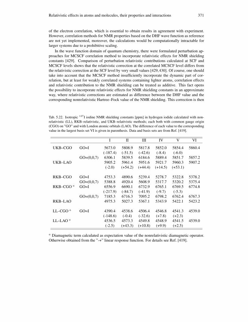
Relativistic effects in atoms and molecules, their properties and interactions 371
of the electron correlation, which is essential to obtain results in agreement with experiment.However, correlation methods for NMR properties based on the DHF wave function as referenceare not yet implemented, moreover, the calculations would be computationally intractable forlarger systems due to a prohibitive scaling.
In the wave function domain of quantum chemistry, there were formulated perturbation ap-proaches for MCSCF correlation method to incorporate relativistic effects for NMR shieldingconstants [429]. Comparison of perturbation relativistic contributions calculated at SCF andMCSCF levels shows that the relativistic correction at the correlated MCSCF level differs fromthe relativistic correction at the SCF level by very small values [429,430]. Of course, one shouldtake into account that the MCSCF method insufficiently incorporate the dynamic part of cor-relation, but at least for weakly correlated systems containing lighter atoms, correlation effectsand relativistic contribution to the NMR shielding can be treated as additive. This fact opensthe possibility to incorporate relativistic effects for NMR shielding constants in an approximateway, where relativistic corrections are estimated as difference between the DHF value and thecorresponding nonrelativistic Hartree–Fock value of the NMR shielding. This correction is then
Tab. 5.22. Isotropic 127I iodine NMR shielding constants [ppm] in hydrogen iodide calculated with non-relativistic (LL), RKB–relativistic, and UKB–relativistic methods; each both with common gauge origin(CGO) on ”GO” and with London atomic orbitals (LAO). The difference of each value to the correspondingvalue in the largest basis set VI is given in parenthesis. Data and basis sets are from Ref. [419].
I II III IV V VI
UKB–CGO GO=I 5673.0 5808.9 5817.8 5852.0 5854.4 5860.4(-187.4) (-51.5) (-42.6) (-8.4) (-6.0)
GO=(0,0,7) 6306.1 5839.5 6184.6 5889.4 5851.7 5857.2UKB–LAO 5905.2 5961.4 5951.6 5921.7 5960.3 5907.2
(-2.0) (+54.2) (+44.4) (+14.5) (+53.1)
RKB–CGO GO=I 4753.3 4890.6 5239.4 5278.7 5322.8 5378.2GO=(0,0,7) 5388.8 4920.4 5608.9 5317.7 5320.2 5375.4
RKB–CGO a GO=I 6556.9 6690.1 6732.9 6765.1 6769.5 6774.8(-217.9) (-84.7) (-41.9) (-9.7) (-5.3)
GO=(0,0,7) 7185.3 6716.3 7095.2 6798.2 6762.4 6767.3RKB–LAO 4975.3 5027.3 5367.1 5343.9 5422.1 5423.2
LL–CGO a GO=I 4390.4 4538.6 4506.4 4546.8 4541.3 4539.0(-148.6) (-0.4) (-32.6) (+7.8) (+2.3)
LL–LAO a 4536.5 4573.3 4549.8 4548.9 4541.5 4539.0(-2.5) (+43.3) (+10.8) (+9.9) (+2.5)
a Diamagnetic term calculated as expectation value of the nonrelativistic diamagnetic operator.Otherwise obtained from the ”-+” linear response function. For details see Ref. [419].

372 Relativistic effects in atomic and molecular properties
added to the nonrelativistic value of the NMR shielding obtained from a high–level correlationmethod like the coupled cluster method [431]. This approach was used for relativistic correctionsof NMR shielding constants for third row hydrides [432] and the results differ by fraction of ppmfrom MCSCF perturbation corrections [430]. Although, spin–spin coupling constants (definedas the second derivative of the energy with respect to magnetic dipoles) correspond to princi-pally different perturbations in the Hamiltonian, this approach is successfully applicable for theseNMR properties as well. The test was performed on spin–spin coupling constants of the group14 XH4 hydrides [433], where authors showed that adding relativistic corrections calculated us-ing the described approximate method to vibrationally corrected nonrelativistic coupled clustervalues of spin–spin coupling constants, J1(XH) (X=C, Si, Ge), leads to an excellent agreementwith gas–phase experimental results. The relativistic correction brought theoretical prediction ofthe spin–spin coupling constant in SnH4 closer to experimental value but the value was overes-timated by about 10%. Although the approach based on additivity of correlation and relativisticeffects gives in some cases better results for NMR properties than relativistic DFT approacheseven for relatively heavy compounds (see, e.g., NMR properties of xenon fluorides [434]), theusage is obviously limited to lighter systems. Moreover, the calculations are quite expensive dueto a slow convergence of the relativistic correction to the basis set limit.
Apart from the mentioned ab initio methods for computing NMR properties there is a largegroup of methods dealing with the electronic correlation and effects of relativity within the two–component DFT approach, see Refs. [435–440].
5.8 From relativistic effects in atoms and molecules to gas–phase properties and thecondensed phase
Relativistic effects, as demonstrated in previous Sections, concern primarily properties of iso-lated atoms or molecules. However, real chemistry and physics proceeds in the gas phase, or,mostly, in the condensed phase. Clearly, the understanding of basic trends in molecular struc-tures, in the bonding character, bonding energies and atomic and molecular properties is un-avoidable for understanding the processes in the gas phase, in solutions and in the solid state,too.
An example of relativistic effects beyond isolated molecules is the investigation of sublima-tion enthalpies of metals in groups 10, 11, and 14 linked with different molecular properties byPershina et al. [441, 442]. Particularly interesting is clear correlation between binding energiesof homonuclear and heteronuclear MM′ diatomics of group 10, 11, and 14 elements with theirsublimation enthalpies. In previous Sections we have presented several examples of a typicalV–shaped pattern of some molecular properties in the series of elements down in the PeriodicTable. The V–shaped pattern characterizes binding energies of the group 10 elements (Ni, Pd,and Pt) and coinage metal elements (Cu, Ag, Au, the group 11). Experimental sublimation en-thalpies ∆Hsub precisely copy the same pattern. Different picture exhibit the group 14 elements.Their binding energies in the Ge, Sn, Pb, and the 114 element series smoothly diminish withincreasing atomic number and precisely the same trend is observed for experimental sublima-tion enthalpies. The behaviour of a series of binding energies of homonuclear and heteronucleardiatomics and relation of these energies to ∆Hsub is analysed using relativistic effects in par-ticipating valence orbitals and their relativistic stabilization (particularly s and p1/2 orbitals) ordestabilization (particularly (n-1)d–orbitals in Hg and the element 112 containing molecules).

Relativistic effects in atoms and molecules, their properties and interactions 373
Comparison of relativistic and nonrelativistic properties of compounds in atomic properties andvolatility of the element 112 and Cd and Hg containing molecules and the V–shaped pattern oftheir properties were treated in detail also in former papers of Pershina et al. [442, 443]. Rela-tivistic effects also affect the adsorption of inert gases, Ne up to Xe, Rn and the element 118 onnoble metal and other surfaces, including quartz, ice, graphite and teflon [444].
A typical V–shaped trend exhibit transfer Gibbs energies of the coinage and alkali metalcations in the combined theoretical and experimental (Secondary Ion Mass Spectrometry, SIMS)research [445] on ion transfer properties in water and acetonitrile. The theoretical ∆G0
298K werebased on the binding energies of the coinage metal Cu+, Ag+, and Au+ cations with waterand acetonitrile obtained from CCSD(T) and DKH–CCSD(T) calculations. Relativistic data donicely correlate with experimental transfer Gibbs energies while the nonrelativistic data are sig-nificantly off this trend. The highest binding energy was found for the Au+ interaction withacetonitrile. This results from the dative sigma–bonding accompanied by the charge transferfrom N to Au+, like it was discussed in detail in Section 5.6 and a significant back–donation ofthe electron density from the Au+ 5d to N 2p shell suggesting the existence of a multiple bondbetween the nitrogen atom and the gold cation. Ilcin et al. [446] performed relativistic CCSD(T)and perturbational calculations of interatomic and intermolecular interactions in complexes ofCdZn, HgZn, and HgCd, and used these data for the temperature dependence of the viscosityfor low–density binary mixtures of the group 12 elements. CCSD(T) spectroscopic constants ofZn2, Cd2, and Hg2 calculated by the DC Hamiltonian give support for an acceptable agreementof theoretical and experimental dynamic viscosities of the Zn, Cd, and Hg vapours [447]. Sim-ilar approach has been used for calculations of diffusion coefficients and stability of Hg· · ·N2
complexes [448].Vogt et al. [449] synthesised and studied experimentally and theoretically the low– and high–
temperature modifications of Sc3RuC4 and Sc3OsC4 carbides. They analysed the local electronicstructure of the T(C2)2 moieties and discussed an interplay between chemical bonding and rela-tivistic effects which is responsible for the ”V”–shaped pattern of the C–C bond length in crystalswith T=Fe, Ru, and Os. Their interpretation includes the T → π∗(C–C) back donation in linewith model M(C2H2) benchmark systems (M=Ni, Pd, and Pt) studied by Ziegler et al. andEickerling et al. [450, 451].
Another new species, the icosahedral WAu12 nanoparticle is a stable multiply bonded systemrepresenting a new structural principle in gold chemistry. Based on the idea of the ”aurophilic-ity” and relativistically strengthened W–Au and Au–Au bonds its existence and properties waspredicted by Pyykko and Runeberg [452] in 2002. The existence of this species was experi-mentally confirmed in the same year [453]. Later on, Pyykko and coworkers [454] studied thefinite–temperature dynamics of this species.
At this occasion we wish to cite the title of the paper ”Gold goes nano – from small clustersto low–dimensional assemblies” in which Schwerdtfeger [351] emphasised that bulk gold is anoble metal but the atomic and nanocrystalline gold compounds can be very reactive and reachapplications in different areas. It was not until 1987 that the interest in gold nanostructures wasreally awakened through the report of Haruta et al. [455] on CO oxidation on supported goldcatalysts. Since then nanocrystalline gold compounds have been the subject of intense researchand have found far reaching applications in areas as catalysis, sensors, molecular electronics or asbioconjugate probes for amplification tags in gene analysis, antibody or antigen detection, DNAsequencing, or gene mapping [351]. Catalytic properties of gold, its ability to create metal–metal

374 Relativistic effects in atomic and molecular properties
bonds, aurophilicity and other phenomena linked with relativistic effects in chemical bonds aspioneered in groups of Pyykko, Schwarz, Schmidbaur, Schwerdtfeger,Schroder and other werediscussed in Section 5.5, see, e.g., Refs. [12, 13, 20, 350–353]. The role of the gold nanofilms inbiomedical applications was analysed by Tokonami et al. [456].
Extremely interesting is discussion of the relation between molecular properties and thesolid–state symmetry. It may help in understanding of experimental observations and sometrends within a group of analogous compounds and their solid state structures, but in any caseit is not straightforward. In two papers dealing with the Cu, Ag, and Au halides Schwerdtfegeret al. [457, 458] compared the structures calculated with and without relativistic effects. Alongwith the bonding characteristics of molecules involved in solid–state structures they also cal-culated sublimation energies for different most stable crystal modifications and their low– andhigh– temperature stabilities and their transitions. Some crystals, like the fluorides CuF, are ex-perimentally unknown since they easily disproportionate at normal conditions. In general, thecoinage halides crystallize in the zinc blende, rock salt or in the chainlike structures. At thenonrelativistic correlated level the cubic structures are favoured. Relativity stabilizes chainlikestructures particularly for the AuX crystals. This is linked with the relativistic increase of the co-valency in Au–X (X is F, Cl, Br, or I) molecules and disfavours in this way ionic structure typesfor which the rock salt crystals are more typical. Different from the AuX compounds, the CuXand AgX halides can be regarded as mainly ionic. How relativity reduces the polarity of MXmolecules is demonstrated in Fig. 5.8. Considerable reduction of the dipole moment is observedparticularly for AuF. The silver halides, which have highest dipole moments, all crystallize atroom temperatures and low pressures in the simple rock salt structure. The most interesting sit-uation is found for the gold halides [458], for which the unusual chainlike structures with shortAu–Au distances are favoured compared to the cubic structures. The main message is [457] thatrelativistic effects drastically influence the solid–state symmetry.
It appears that similar analysis as was presented for the group 11 monohalides is also appli-cable to the group 12 solid–state oxides, ZnO, CdO, and HgO [459]. The solid–state HgO atlow pressure is analogous with the AuF structure. It is represented by the chainlike montroyditeand cinnabar structures in contrast with ZnO and CdO structures which have typically hexagonalwurtzite or rock salt structures. This marked difference is caused by relativistic effects. Thereis some analogy between the bonding situation in AuF and HgO. As it is presented in Tab. 5.19,the bond strength of both molecules is significantly relativistically reduced, and, also, both mole-cules become less polar, i.e. their dipole moments diminish due to relativistic effects, see Fig. 5.8and Refs. [300, 459]. Besides of changes in the solid–state structure, relativistic effects also re-duce the cohesive energy of HgO. It appears that the unusual yellow to red colour of HgO is arelativistic effect as well [459].
Exceptional position of Hg containing crystals in the group 12 dihalides is also attributedto relativistic effects by Donald et al. [414]. Their analysis is based on DFT calculations ofmonomers and dimers of MX2 molecules (M = Zn, Cd, Hg and X = F, Cl, Br, I). The zinc andcadmium dihalide dimers have the usual D2h symmetry geometry, whereas the mercury dihalidedimers are loosely–bound units with the C2h symmetry. Donald et al. found an obvious con-nection between the structures and characteristics of monomers, their dimers, and the crystalsthey form. The crystal structures of the group 12 MX2 dihalides exhibit a wide range of struc-tural types, from three–dimensional extended solids to molecular crystals. Since the ionizationpotential of Hg is high due to the relativistic stabilization of its valence 6s2 electrons, somewhat

Relativistic effects in atoms and molecules, their properties and interactions 375
surprising is the structure of HgF2, which becomes an ionic solid. The crystals of HgCl2 andHgBr2 are molecular solids which is connected with smaller electronegativity of Cl and Br sothat extended structures cannot be formed.
Calculations [460] of the interatomic interaction energies for the Hg dimer and small clustersof the mercury atoms allowed to develop a many–body expansion of the correlation energy whichis added to the solid state HF energy [461]. The Hg dimer is more strongly bound than the Znand Cd dimers due to relativistic effects. The cluster studies were extended to the solid state andoptimized lattice parameters and cohesive energies for bulk mercury. For smaller clusters thehighly accurate CCSD(T) method was still applicable. DFT methods applicable to larger clusterslead to diverse results for, e.g., the cohesive energies for bulk mercury. Accurate interactionpotentials including at least three–body effects are critically needed for reliable description ofthe bulk properties by Monte Carlo simulations [462]. Accurate interaction potentials, based onthe fitting of CCSD(T) data, lead to excellent agreement of the bulk melting temperature of argon,84.7 K, within less than 1 K of the experimental value. Such accuracy is not yet achievable formetallic systems or molecular solids, but preliminary results results are at least very promising.
A cluster modelling of the interaction of the eka-Hg (element 112) and eka–Pb atom (element114) with the stable Au(111) surface using accurate small–core relativistic pseudopotentials andtwo–component non–collinear DFT was published by Zaitsevskii et al. [416, 463].

376 Relativistic effects in atomic and molecular properties
6 Conclusions
Real life of molecules is a relativistic quantum mechanical life. This holds for all atoms andmolecules throughout the Periodic Table. In light elements are relativistic effects visible in finestructure effects and are growing dramatically for molecules containing elements with increasingatomic number. We have demonstrated that relativistic effects alter many atomic and molecularproperties not only quantitatively but also qualitatively. Most important aspect of this paper isunderstanding of trends within the Periodic Table. For specific groups of elements in the Ta-ble we analyse trends of ionization potentials, electron affinities, geometries, electric properties,magnetic properties, interaction and reaction energies. When going to heavier atoms relativis-tic effects lead frequently to characteristic ”V” shaped behaviour of properties with respect tothe atomic number. These relativistic changes are related to the electronic structure of atomsand molecules. We also discuss briefly the link between relativistic changes in properties ofindividual atoms or molecules and their behaviour in the condensed phase.
We are witnessing vigorous progress in the development of new relativistic theoretical ap-proaches and methods, which allow treating of gradually larger many–electron molecules at thecorrelated relativistic level with a reasonable accuracy. Both wave function and density func-tional theories participate on the extension of applicability to a wide scale of problems whichneed and can be treated by relativistic methods of quantum chemistry.
Acknowledgments
This research was supported by the Slovak Grant Agency, grant VEGA–1/0520/10 and grants ofthe Slovak Research and Development Agency APVV (Contracts No. LPP–0110–07 and LPP–0155–09). We are grateful to Professor Maria Barysz, Dr. Lukas Bucinsky, Assoc. ProfessorPavel Neogrady, and Professor Jan Pisut for careful reading the manuscript, for their valuablesuggestions and their kind help in correcting inaccuracies in the text. We also acknowledge theeffort of Professor Vladimır Buzek for his enthusiastic pushing for finishing this paper.

Conclusions 377
Appendix: Atomic units
Introducing atomic units, e = m0 = h = 4πε0 = 1, considerably simplifies all formulae ofquantum mechanics. In Tab. 0.1 we present SI values of atomic units.
Tab. 0.1. The conversion factors of atomic units to SI and other units based on the 2006 CODATA adjust-ment of the value of constants [45].
a.u. of Symbol Numerical value Unit
charge: elementary charge e 1.602 176 487(40)×10−19 Cmass: electron mass me 9.109 382 15(45)×10−31 kgaction: reduced Planck constant h 1.054 571 628(53)×10−34 J slength: Bohr radius (bohr) a0 0.529 177 208 59(36)×10−10 m
0.529 177 208 59(36)×10−10 Aenergy: Hartree energy (hartree) Eh 4.359 743 94(22)×10−18 J
27.211 383 86(68) eV2.194 746 313 705(15)×105 cm−1
2.625 499 617×103 kJ mol−1
time h/Eh 2.418 884 326 505(16)×10−17 sforce Eh/a0 8.238 722 06(41)×10−8 Nvelocity a0Eh/h 2.187 691 2541(15)×106 m s−1
momentum h/a0 1.992 851 565(99)×10−24 kg m s−1
current eEh/h 6.623 617 63(17)×10−3 Acharge density e/a3
0 1.081 202 300(27)×1012 C m−3
electric potential Eh/e 27.211 383 86(68) Velectric field Eh/ea0 5.142 206 32(13)×1011 V m−1
electric field gradient Eh/ea20 9.717 361 66(24)×1021 V m−2
electric dipole moment ea0 8.478 352 81(21)×10−30 C m2.541 746 23 Debye
electric quadrupole moment ea20 4.486 551 07(11)×10−40 C m2
electric polarizability e2a20/Eh 1.648 777 2536(34)×10−41 C2 m2 J−1
1st hyperpolarizability e3a30/E
2h 3.206 361 533(81)×10−53 C3 m3 J−2
2nd hyperpolarizability e4a40/E
3h 6.235 380 95(31)×10−65 C4 m4 J−3
magnetic flux density h/ea20 2.350 517 382(59)×105 T
magnetic dipole moment he/me 1.854 801 830(46)×10−23 J T−1
magnetizability e2a20/me 7.891 036 433(27)×10−29 J T−2
permitivity e2/a0Eh 1.112 650 056...×10−10 F m−1

378 Relativistic effects in atomic and molecular properties
References
[1] S. L. Glashow, B. Bova: Interactions : a journey through the mind of a particle physicist and thematter of this world: Warner Books, New York, NY (1988)
[2] P. A. M. Dirac: Proc. Roy. Soc. Lond. A 123 (1929) 714[3] W. Heitler, F. London: Z. Phys. 44 (1927) 455[4] P. A. M. Dirac: Proc. Roy. Soc. Lond. A 117 (1928) 610[5] W. Kołos, L. Wolniewicz: Acta Phys. Polon. 20 (1961) 129[6] B. Swirles: Proc. Roy. Soc. Lond. A 152 (1935) 625[7] I. P. Grant: Proc. Roy. Soc. Lond. A 262 (1961) 555[8] J. P. Desclaux: At. Data Nucl. Data Tabes 12 (1973) 311[9] P. Pyykko, J. P. Desclaux: Accounts Chem. Res. 12 (1979) 276
[10] P. Pyykko: Chem. Rev. 88 (1988) 563[11] P. Pyykko: Chem. Rev. 97 (1997) 597[12] P. Pyykko: Angew. Chem.-Int. Edit. 41 (2002) 3573[13] P. Pyykko: Angew. Chem.-Int. Edit. 43 (2004) 4412[14] W. Kutzelnigg: Phys. Rev. A 54 (1996) 1183[15] J. Almlof, O. Gropen: In: Reviews in computational chemistry, eds. K. B. Lipkowitz, D. B. Boyd,
vol. 8, pp. 203–244. Willey-VCH, New York (2001)[16] P. Schwerdtfeger: In: Atoms, Molecules and Clusters in Electric fields: Theoretical Approaches to
the calculation of electric polarizability, ed. G. Maroulis, pp. 1–32. Imperial College Press, London(2006)
[17] P. Schwerdtfeger, M. Seth: In: Encyclopedia of Computational Chemistry, ed. P. v. R. Schleyer, pp.2480–2499. Wiley, Chichester (1998)
[18] B. A. Hess: In: Encyclopedia of Computational Chemistry, ed. P. v. R. Schleyer, pp. 2499–2508.Wiley, Chichester (1998)
[19] W. H. E. Schwarz, A. Rutkowski, S. G. Wang: Int. J. Quantum Chem. 57 (1996) 641[20] H. Schwarz: Angew. Chem.-Int. Edit. 42 (2003) 4442[21] M. Urban, V. Kello: Adv. Quantum Chem. 50 (2005) 249[22] M. Urban, V. Kello: Comput. Lett. 2 (2006) 259[23] P. Schwerdtfeger (ed.): Relativistic electronic structure theory. Part 1. Fundamentals.: Theoretical
and computational chemistry v. 11. Elsevier, Amsterdam (2002)[24] P. Schwerdtfeger (ed.): Relativistic electronic structure theory. Part 2. Applications.: Theoretical
and computational chemistry v. 14. Elsevier, Amsterdam (2004)[25] K. G. Dyall, K. Fægri: Introduction to relativistic quantum chemistry: Oxford University Press,
New York (2007)[26] M. Reiher, A. Wolf: Relativistic quantum chemistry : the fundamental theory of molecular science:
Wiley-VCH, Weinheim (2009)[27] P. A. M. Dirac: Proc. Roy. Soc. Lond. A 118 (1928) 351[28] I. P. Grant, H. M. Quiney: Int. J. Quantum Chem. 80 (2000) 283[29] K. Pachucki, J. Komasa: Phys. Rev. Lett. 92 (2004) 213001[30] D. Mendeleev: Zhurnal Russkoe Fiziko-Khimicheskoe Obshchestvo 1 (1869) 66[31] D. Mendelejeff: Zeitschrift fur Chemie 12 (1869) 405

References 379
[32] D. R. Lide (ed.): CRC handbook of chemistry and physics, CD-ROM Version 2005: CRC Press,Boca Raton (2005)
[33] P. Neogrady, V. Kello, M. Urban, A. J. Sadlej: Int. J. Quantum Chem. 63 (1997) 557[34] J. Gazo, J. Kohout, M. Serator, T. Sramko, M. Zikmund: Vseobecna a anorganicka chemia: Alfa,
Bratislava (1974)[35] M. Urban, J. Noga, S. J. Cole, R. J. Bartlett: J. Chem. Phys. 83 (1985) 4041[36] K. Raghavachari, G. W. Trucks, J. A. Pople, M. HeadGordon: Chem. Phys. Lett. 157 (1989) 479[37] M. Urban, I. Cernusak, J. Noga, V. Kello: In: Methods in Computational Chemistry, ed. S. Wilson,
vol. 1, pp. 117–250. Plenum Press, New York (1987)[38] J. Paldus, X. Z. Li: Adv. Quantum Chem. 110 (1999) 1[39] T. Helgaker, P. Jørgensen, J. Olsen: Molecular electronic-structure theory: Wiley, Chichester ; New
York (2000)[40] I. Shavitt, R. J. Bartlett: Many-body methods in chemistry and physics : MBPT and coupled-cluster
theory: Cambridge molecular science. Cambridge University Press, Cambridge ; New York (2009)[41] J. P. Desclaux, Y. K. Kim: J. Phys. B-At. Mol. Opt. Phys. 8 (1975) 1177[42] N. Bohr: Philos. Mag. 26 (1913) 1[43] A. Einstein: Ann. Phys.-Berlin 17 (1905) 891[44] J. C. Maxwell: Philos. Mag. 21 (1861) 161[45] P. J. Mohr, B. N. Taylor, D. B. Newell: Rev. Mod. Phys. 80 (2008) 633[46] J. F. Harrison: Spin–orbit interaction (2006): http://www.cem.msu.edu/˜cem987/spin orbit.pdf[47] E. Schrodinger: Phys. Rev. 28 (1926) 1049[48] W. Gerlach, O. Stern: Z. Phys. 9 (1922) 353[49] G. E. Uhlenbeck, S. Goudsmit: Nature 117 (1926) 264[50] J. Pisut, R. Zajac: O atomoch a kvantovanı: FMFI UK, Bratislava (2009)[51] L. Piela: Ideas of quantum chemistry: Elsevier, Amsterdam ; Boston (2007)[52] G. E. Uhlenbeck, S. Goudsmit: Naturw. 13 (1925) 953[53] W. Pauli: Z. Phys. 43 (1927) 601: See footnote 2 on page 607[54] M. Born, R. Oppenheimer: Ann. Phys.-Berlin 84 (1927) 0457[55] J. C. Slater: Phys. Rev. 34 (1929) 1293[56] V. Fock: Z. Phys. 61 (1930) 126[57] D. R. Hartree, W. Hartree: Proc. Roy. Soc. Lond. A 150 (1935) 9[58] D. R. Hartree: Nature 138 (1936) 1080[59] C. C. J. Roothaan: Rev. Mod. Phys. 32 (1960) 179[60] J. A. Pople, R. K. Nesbet: J. Chem. Phys. 22 (1954) 571[61] S. F. Boys: Proc. R. Soc. London Ser. A 200 (1950) 542[62] P. Carsky, M. Urban: Ab initio calculations : methods and applications in chemistry: Lecture notes
in chemistry 16. Springer-Verlag, Berlin ; New York (1980)[63] C. C. J. Roothaan: Rev. Mod. Phys. 23 (1951) 69[64] F. Aquilante, L. De Vico, N. Ferre, G. Ghigo, P.-A. Malmqvist, P. Neogrady, T. B. Pedersen,
M. Pitonak, M. Reiher, B. O. Roos, L. Serrano-Andres, M. Urban, V. Veryazov, R. Lindh: J. Comput.Chem. 31 (2010) 224
[65] M. Urban, P. Neogrady, I. Hubac: In: Recent Advances in Computational Chemistry, ed. R. J.Bartlett, vol. 3, pp. 275–306. World Scientific, Singapore (1997)

380 Relativistic effects in atomic and molecular properties
[66] J. D. Watts, J. Gauss, R. J. Bartlett: J. Chem. Phys. 98 (1993) 8718[67] P.-O. Lowdin: Phys. Rev. 97 (1955) 1509[68] C. D. Sherrill, H. F. Schaefer: Adv. Quantum Chem. 34 (1999) 143[69] B. Roos: Chem. Phys. Lett. 15 (1972) 153[70] M. Barbatti, H. Lischka: J. Phys. Chem. A 111 (2007) 2852[71] T. D. Crawford, H. F. Schaefer: In: Reviews in Computational Chemistry, eds. K. B. Lipkowitz,
D. B. Boyd, pp. 33–136. Wiley-VCH, Inc., Hoboken (2007)[72] M. Gell-Mann, K. A. Brueckner: Phys. Rev. 106 (1957) 364[73] H. A. Bethe: Phys. Rev. 103 (1956) 1353[74] F. Coester: Nucl. Phys. 7 (1958) 421[75] F. Coester, H. Kummel: Nucl. Phys. 17 (1960) 477[76] J. Cızek: J. Chem. Phys. 45 (1966) 4256[77] J. Cızek: Adv. Chem. Phys. 14 (1969) 35[78] J. Paldus, I. Shavitt, J. Cızek: Phys. Rev. A 5 (1972) 50[79] R. J. Bartlett: J. Phys. Chem. 93 (1989) 1697[80] J. Paldus, J. Cızek: Adv. Quantum Chem. 9 (1975) 105[81] J. Paldus: In: Methods in Computational Molecular Physics, eds. S. Wilson, G. H. F. Diercksen, vol.
293 of NATO Advanced Science Institutes Series, Series B, Physics, pp. 99–194. Plenum Press, NewYork (1992)
[82] S. A. Kucharski, R. J. Bartlett: Theor. Chim. Acta 80 (1991) 387[83] I. Lindgren, S. Salomonson, D. Hedendahl: In: Recent progress in coupled cluster methods: Theory
and applications, eds. P. Carsky, J. Paldus, J. Pittner, pp. 357–374. Springer, Berlin (2010)[84] E. Eliav, U. Kaldor: In: Recent progress in coupled cluster methods: Theory and applications, eds.
P. Carsky, J. Paldus, J. Pittner, pp. 113–144. Springer, Berlin (2010)[85] P. Carsky, J. Paldus, J. Pittner (eds.): Recent progress in coupled cluster methods: Theory and
applications: Springer, Berlin (2010)[86] G. D. Purvis, R. J. Bartlett: J. Chem. Phys. 76 (1982) 1910[87] J. Noga, R. J. Bartlett: J. Chem. Phys. 86 (1987) 7041[88] R. J. Bartlett, M. Musial: Rev. Mod. Phys. 79 (2007) 291[89] M. Kallay, P. R. Surjan: J. Chem. Phys. 115 (2001) 2945[90] S. A. Kucharski, R. J. Bartlett: J. Chem. Phys. 108 (1998) 5243[91] M. Musial, S. A. Kucharski, R. J. Bartlett: J. Chem. Phys. 116 (2002) 4382[92] X. Z. Li, J. Paldus: J. Chem. Phys. 101 (1994) 8812[93] P. Neogrady, M. Urban: Int. J. Quantum Chem. 55 (1995) 187[94] M. Douglas, N. M. Kroll: Ann. Phys. (N.Y.) 82 (1974) 89[95] B. A. Hess: Phys. Rev. A 32 (1985) 756[96] J. Noga, W. Kutzelnigg: J. Chem. Phys. 101 (1994) 7738[97] X. Z. Li, J. Paldus: J. Chem. Phys. 119 (2003) 5320[98] J. Pittner, P. Piecuch: Mol. Phys. 107 (2009) 1209[99] O. Demel, J. Pittner, P. Carsky, I. Hubac: J. Phys. Chem. A 108 (2004) 3125
[100] B. O. Roos, K. Andersson, M. P. Fulscher, P.-A. Malmqvist, L. Serrano-Andres, K. Pierloot,M. Merchan: Adv. Chem. Phys. 93 (1996) 219

References 381
[101] K. Andersson, P.-A. Malmqvist, B. O. Roos, A. J. Sadlej, K. Wolinski: J. Phys. Chem. 94 (1990)5483
[102] B. O. Roos, P.-A. Malmqvist: Phys. Chem. Chem. Phys. 6 (2004) 2919[103] P.-A. Malmqvist, B. O. Roos, B. Schimmelpfennig: Chem. Phys. Lett. 357 (2002) 230[104] Z. Azizi, B. O. Roos, V. Veryazov: Phys. Chem. Chem. Phys. 8 (2006) 2727[105] B. O. Roos, R. Lindh, P.-A. Malmqvist, V. Veryazov, P. O. Widmark: J. Phys. Chem. A 108 (2004)
2851[106] B. O. Roos, R. Lindh, P.-A. Malmqvist, V. Veryazov, P. O. Widmark: J. Phys. Chem. A 109 (2005)
6575[107] H. A. Lorentz: Proc. Acad. Science Amsterdam 1 (1899) 427[108] H. Poincare: Comptes rendus de l’ Academie des Sciences de Paris 140 (1905) 1504[109] A. Einstein: Ann. Phys.-Berlin 18 (1905) 639[110] W. Gordon: Z. Phys. 40 (1926) 117[111] O. Klein: Z. Phys. 41 (1927) 407[112] W. Pauli, V. Weisskopf: Helv. Phys. Acta 7 (1934) 709[113] P. A. M. Dirac: In: History of twentieth century physics, ed. C. Weiner, pp. 109–146. Academic
Press, New York (1977)[114] C. D. Anderson: Phys. Rev. 41 (1932) 405[115] C. G. Darwin: Proc. Roy. Soc. Lond. A 118 (1928) 654[116] H. A. Bethe, E. E. Salpeter: Quantum mechanics of one-and two-electron atoms: Plenum Press,
New York (1977)[117] R. E. Moss: Advanced molecular quantum mechanics; an introduction to relativistic quantum me-
chanics and the quantum theory of radiation: Chapman and Hall, London (1973)[118] M. E. Rose: Relativistic electron theory: Wiley, New York (1961)[119] A. Messiah: Quantum mechanics: North-Holland, Amsterdam (1961)[120] H. E. White: Phys. Rev. 38 (1931) 514[121] A. Szabo: J. Chem. Educ. 46 (1969) 678[122] C. W. Sherwin: Introduction to quantum mechanics: Holt, Rinehart and Winston, New York (1959)[123] I. P. Grant, H. M. Quiney: Adv. At. Mol. Phys. 23 (1988) 37[124] Y. Ishikawa, H. M. Quiney: Int. J. Quantum Chem. Suppl. 21 (1987) 523[125] O. Visser, P. J. C. Aerts, D. Hegarty, W. C. Nieuwpoort: Chem. Phys. Lett. 134 (1987) 34[126] L. Visscher, K. G. Dyall: At. Data Nucl. Data Tables 67 (1997) 207: see also
http://www.chem.vu.nl/˜visscher/FiniteNuclei/FiniteNuclei.htm[127] M. Gell-Mann: Nuovo Cimento Suppl. 4 (1956) 848[128] T. Saue, L. Visscher: In: Theoretical chemistry and physics of heavy and superheavy elements,
eds. U. Kaldor, S. Wilson, vol. 11 of Progress in theoretical chemistry and physics, p. 211. Kluwer,Dordrecht (2003)
[129] P. A. M. Dirac: In: Structure et Propertietes des Noyaux Atomiques. Septieme Conseil du PhysiqueSolvay, Bruxelles, 22–29 October 1933, eds. J. Cockcroft, J. Chadwick, F. Joliot, J. Joliot, N. Bohr,G. Gamov, P. A. M. Dirac, W. Heisenberg, pp. 203–230. Gautier-Villars, Paris (1934)
[130] G. Breit: Physical Review 34 (1929) 553[131] J. A. Gaunt: Proc. Roy. Soc. Lond. A 122 (1929) 513[132] P. M. Kozlowski, L. Adamowicz: Chem. Rev. 93 (1993) 2007

382 Relativistic effects in atomic and molecular properties
[133] G. E. Brown, D. G. Ravenhall: Proc. Roy. Soc. Lond. A 208 (1951) 552[134] M. H. Mittleman: Phys. Rev. A 24 (1981) 1167[135] H. M. Quiney: Private communication; the information is provided in a letter from Lady Jeffreys
(born Swirles) to H.M.Q., 3 March 1997 ()[136] G. Malli, J. Oreg: J. Chem. Phys. 63 (1975) 830[137] R. E. Stanton, S. Havriliak: J. Chem. Phys. 81 (1984) 1910[138] P. J. C. Aerts, W. C. Nieuwpoort: Chem. Phys. Lett. 113 (1985) 165[139] K. G. Dyall, I. P. Grant, S. Wilson: J. Phys. B-At. Mol. Opt. Phys. 17 (1984) 493[140] L. Visscher, P. J. C. Aerts, O. Visser: In: The effects of relativity in atoms, molecules, and the solid
state, eds. S. Wilson, I. P. Grant, B. L. Gyorffy, p. 197. Plenum Press, New York (1991)[141] J. Thyssen: Develompment and applications of methods for correlated relativistic calculations of
molecular properties: Phd. thesis, University of Southern Denmark, Odense (2001)[142] H. J. Aa. Jensen, K. G. Dyall, T. Saue, K. Fægri: J. Chem. Phys. 104 (1996) 4083[143] J. Thyssen, T. Fleig, H. J. Aa. Jensen: J. Chem. Phys. 129 (2008) 034109[144] T. Fleig, C. M. Marian, J. Olsen: Theor. Chem. Acc. 97 (1997) 125[145] H. A. Kramers: Proc. Acad. Sci. Amsterdam 33 (1930) 959[146] P. Hafner: J. Phys. B-At. Mol. Opt. Phys. 13 (1980) 3297[147] H. A. Bethe: Annal. Phys. 3 (1929) 133208[148] S. L. Altmann: Rotations, quaternions, and double groups: Clarendon Press, Oxford (1986)[149] C. J. Bradley, A. P. Cracknell: The mathematical theory of symmetry in solids; representation theory
for point groups and space groups: Clarendon Press, Oxford, (1972)[150] P. J. C. Aerts: Chem. Phys. Lett. 104 (1984) 28[151] A. Rosen: Int. J. Quantum Chem. 13 (1978) 509[152] J. Meyer: Int. J. Quantum Chem. 33 (1988) 445[153] J. Meyer, W. D. Sepp, B. Fricke, A. Rosen: Comput. Phys. Commun. 54 (1989) 55[154] L. Visscher: Chem. Phys. Lett. 253 (1996) 20[155] T. Saue, H. J. Aa. Jensen: J. Chem. Phys. 111 (1999) 6211[156] K. Rykhlinskaya, S. Fritzsche: Comput. Phys. Commun. 171 (2005) 119[157] T. Yanai, R. J. Harrison, T. Nakajima, Y. Ishikawa, K. Hirao: Int. J. Quantum Chem. 107 (2007)
1382[158] D. L. Peng, J. Y. Ma, W. J. Liu: Int. J. Quantum Chem. 109 (2009) 2149[159] B. A. Hess, C. M. Marian: In: Computational molecular spectroscopy, eds. P. Jensen, P. R. Bunker,
p. 169. Wiley, Chichester ; New York (2000)[160] K. Balasubramanian: Relativistic effects in chemistry. Part A: Theory and techniques: Wiley Inter-
science, New York (1997)[161] K. G. Dyall: Theor. Chem. Acc. 115 (2006) 441[162] K. G. Dyall: Theor. Chem. Acc. 117 (2007) 483[163] K. G. Dyall: J. Phys. Chem. A 113 (2009) 12638[164] K. G. Dyall, A. S. P. Gomes: Theor. Chem. Acc. 125 (2010) 97[165] A. Gomes, K. Dyall, L. Visscher: Theor. Chem. Acc. (2010): DOI 10.1007/s00214-009-0725-7[166] L. Visscher: Theor. Chem. Acc. 98 (1997) 68[167] M. Abe, T. Yanai, T. Nakajima, K. Hirao: Chem. Phys. Lett. 388 (2004) 68[168] C. Møller, M. Plesset: Phys. Rev. 46 (1934) 618

References 383
[169] J. K. Laerdahl, T. Saue, K. Fægri: Theor. Chem. Acc. 97 (1997) 177[170] DIRAC: a relativistic ab initio electronic structure program, release dirac08 (2008): written by
L. Visscher, H. J. Aa. Jensen, and T. Saue, with new contributions from R. Bast, S. Dubillard,K. G. Dyall, U. Ekstrom, E. Eliav, T. Fleig, A. S. P. Gomes, T. U. Helgaker, J. Henriksson, M. Ilias,Ch. R. Jacob, S. Knecht, P. Norman, J. Olsen, M. Pernpointner, K. Ruud, P. Sałek, and J. Sikkema,see http://dirac.chem.sdu.dk
[171] M. Abe, T. Nakajima, K. Hirao: J. Chem. Phys. 125 (2006) 234110[172] L. Visscher, T. J. Lee, K. G. Dyall: J. Chem. Phys. 105 (1996) 8769[173] M. Pernpointner, L. Visscher: J. Comput. Chem. 24 (2003) 754[174] L. Visscher, K. G. Dyall, T. J. Lee: Int. J. Quantum Chem. Suppl. 29 (1995) 411[175] A. Landau, E. Eliav, Y. Ishikawa, U. Kaldor: J. Chem. Phys. 121 (2004) 6634[176] L. Visscher, E. Eliav, U. Kaldor: J. Chem. Phys. 115 (2001) 9720[177] A. Landau, E. Eliav, U. Kaldor: Chem. Phys. Lett. 313 (1999) 399[178] A. Landau, E. Eliav, U. Kaldor: Int. J. Mod. Phys. B 17 (2003) 5335[179] E. Eliav, M. J. Vilkas, Y. Ishikawa, U. Kaldor: J. Chem. Phys. 122 (2005) 224113[180] T. Fleig, J. Olsen, C. M. Marian: J. Chem. Phys. 114 (2001) 4775[181] T. Fleig, J. Olsen, L. Visscher: J. Chem. Phys. 119 (2003) 2963[182] T. Fleig, H. J. Aa. Jensen, J. Olsen, L. Visscher: J. Chem. Phys. 124 (2006) 104106[183] S. Knecht, H. J. Aa. Jensen, T. Fleig: J. Chem. Phys. 132 (2010) 014108[184] T. Fleig: Phys. Rev. A 77 (2008) 062503[185] Y. S. Lee: In: Relativistic electronic structure theory. Part 2. Applications., ed. P. Schwerdtfeger,
Theoretical and computational chemistry v. 14, pp. 352–416. Elsevier, Amsterdam (2004)[186] K. A. Peterson, D. Figgen, E. Goll, H. Stoll, M. Dolg: J. Chem. Phys. 119 (2003) 11113[187] D. Figgen, K. A. Peterson, M. Dolg, H. Stoll: J. Chem. Phys. 130 (2009) 164108[188] H. Stoll: Chem. Phys. Lett. 429 (2006) 289[189] D. Figgen, A. Wedig, H. Stoll, M. Dolg, E. Eliav, U. Kaldor: J. Chem. Phys. 128 (2008) 024106[190] L. L. Foldy, S. A. Wouthuysen: Phys. Rev. 78 (1950) 29[191] B. A. Hess, C. M. Marian, S. D. Peyerimhoff: In: Modern electronic structure theory, Part I, ed. D. R.
Yarkony, Advanced series in physical chemistry, Vol. 2, pp. 152–278. World Scientific, Singapore(1995)
[192] B. A. Hess: Phys. Rev. A 33 (1986) 3742[193] T. Nakajima, K. Hirao: J. Chem. Phys. 113 (2000) 7786[194] T. Nakajima, K. Hirao: J. Chem. Phys. 119 (2003) 4105[195] C. Park, J. E. Almlof: Chem. Phys. Lett. 231 (1994) 269[196] C. van Wullen: J. Chem. Phys. 120 (2004) 7307[197] M. Reiher, A. Wolf: J. Chem. Phys. 121 (2004) 2037[198] M. Reiher, A. Wolf: J. Chem. Phys. 121 (2004) 10945[199] J. L. Heully, I. Lindgren, E. Lindroth, S. Lundqvist, A. M. Martensson-Pendrill: J. Phys. B-At. Mol.
Opt. Phys. 19 (1986) 2799[200] W. Kutzelnigg: J. Chem. Phys. 110 (1999) 8283[201] W. Kutzelnigg, W. J. Liu: J. Chem. Phys. 123 (2005) 241102[202] E. van Lenthe, E. J. Baerends, J. G. Snijders: J. Chem. Phys. 105 (1996) 2373[203] K. G. Dyall: J. Chem. Phys. 106 (1997) 9618

384 Relativistic effects in atomic and molecular properties
[204] K. G. Dyall: In: Theoretical chemistry and physics of heavy and superheavy elements, eds.U. Kaldor, S. Wilson, p. 325. Kluwer, Dordrecht (2003)
[205] C. Chang, M. Pelissier, P. Durand: Phys. Scr. 34 (1986) 394[206] E. van Lenthe, E. J. Baerends, J. G. Snijders: J. Chem. Phys. 101 (1994) 9783[207] E. van Lenthe, J. G. Snijders, E. J. Baerends: J. Chem. Phys. 105 (1996) 6505[208] K. G. Dyall, E. van Lenthe: J. Chem. Phys. 111 (1999) 1366[209] R. van Leeuwen, E. van Lenthe, E. J. Baerends, J. G. Snijders: J. Chem. Phys. 101 (1994) 1272[210] Y. Nakatsuka, T. Nakajima, M. Nakata, K. Hirao: J. Chem. Phys. 132 (2010) 054102[211] M. Barysz, A. J. Sadlej, J. G. Snijders: Int. J. Quantum Chem. 65 (1997) 225[212] M. Barysz, A. J. Sadlej: Theochem-J. Mol. Struct. 573 (2001) 181[213] M. Barysz: J. Chem. Phys. 114 (2001) 9315[214] M. Barysz, A. J. Sadlej: J. Chem. Phys. 116 (2002) 2696[215] M. Barysz: In: Theoretical Chemistry and Physics of Heavy and Super-Heavy Elements., eds.
U. Kaldor, S. Wilson, vol. 11 of Progress in Theoretical Chemistry and Physics, pp. 349–397. KluwerAcademic Publishers, Dordrecht (2003)
[216] M. Barysz: In: Relativistic methods for chemists, eds. M. Barysz, Y. Ishikawa, vol. 10 of Challengesand advances in computational chemistry and physics, pp. 165–190. Springer, Dordrecht (2010)
[217] R. D. Cowan, D. C. Griffin: J. Opt. Soc. Am. 66 (1976) 1010[218] J. H. Wood, A. M. Boring: Phys. Rev. B 18 (1978) 2701[219] S. Komorovsky, M. Repisky, O. L. Malkina, V. G. Malkin, I. Malkin, M. Kaupp: J. Chem. Phys.
124 (2006) 084108[220] V. Kello, A. J. Sadlej: Int. J. Quantum Chem. 68 (1998) 159[221] M. Barysz: Pol. J. Chem. 74 (2000) 1329[222] D. Kedziera, M. Barysz, A. J. Sadlej: Struct. Chem. 15 (2004) 369[223] J. Seino, W. Uesugi, M. Hada: J. Chem. Phys. 132 (2010) 164108[224] M. Ilias, T. Saue: J. Chem. Phys. 126 (2007) 064102[225] L. Visscher, T. Saue: J. Chem. Phys. 113 (2000) 3996[226] K. G. Dyall: J. Chem. Phys. 100 (1994) 2118[227] H. J. Aa. Jensen, M. Ilias in preparation[228] W. J. Liu, D. L. Peng: J. Chem. Phys. 125 (2006) 044102[229] D. Kedziera, M. Barysz: Chem. Phys. Lett. 446 (2007) 176[230] M. Barysz, L. Mentel, J. Leszczynski: J. Chem. Phys. 130 (2009) 164114[231] C. E. Moore: Ionization Potentials and Ionization Limits Derived from the Analyses of Optical
Spectra: Natl. Stand. Ref. Data Ser. U.S. Natl. Bur. Stand. (1970)[232] T. Saue, H. J. Aa. Jensen: J. Chem. Phys. 118 (2003) 522[233] C. M. Marian: In: Reviews in computational chemistry, eds. K. B. Lipkowitz, D. B. Boyd, vol. 17,
pp. 99–204. Willey-VCH, New York (2001)[234] B. A. Hess, C. M. Marian, U. Wahlgren, O. Gropen: Chem. Phys. Lett. 251 (1996) 365[235] M. Ilias, V. Kello, L. Visscher, B. Schimmelpfennig: J. Chem. Phys. 115 (2001) 9667[236] L. Visscher, O. Visser, P. J. C. Aerts, H. Merenga, W. C. Nieuwpoort: Comput. Phys. Commun. 81
(1994) 120[237] H. N. Russel, F. A. Saunders: Astrophys. J. 61 (1925) 38[238] W. E. Lamb, R. C. Retherford: Phys. Rev. 72 (1947) 241

References 385
[239] H. A. Bethe: Phys. Rev. 72 (1947) 339[240] J. P. Briand, P. Chevallier, P. Indelicato, K. P. Ziock, D. D. Dietrich: Phys. Rev. Lett. 65 (1990) 2761[241] I. Goidenko, L. Labzowsky, E. Eliav, U. Kaldor, P. Pyykko: Phys. Rev. A 67 (2003) 020102[242] K. G. Dyall, C. W. Bauschlicher, D. W. Schwenke, P. Pyykko: Chem. Phys. Lett. 348 (2001) 497[243] M. J. Vilkas, Y. Ishikawa, K. Hirao: Chem. Phys. Lett. 321 (2000) 243[244] T. H. Dunning, K. A. Peterson, D. E. Woon: In: Encyclopedia of Computational Chemistry, ed.
P. v. R. Schleyer, pp. 88–115. Wiley, Chichester (1998)[245] A. J. Sadlej: Collect. Czech. Chem. Commun. 53 (1988) 1995[246] A. J. Sadlej: Theor. Chim. Acta 79 (1991) 123[247] A. J. Sadlej, M. Urban: Theochem-J. Mol. Struct. 234 (1991) 147[248] A. J. Sadlej, M. Urban, O. Gropen: Phys. Rev. A 44 (1991) 5547[249] A. J. Sadlej: Theor. Chim. Acta 81 (1991) 45[250] A. J. Sadlej: Theor. Chim. Acta 81 (1992) 339[251] V. Kello, A. J. Sadlej: Theor. Chim. Acta 83 (1992) 351[252] V. Kello, A. J. Sadlej, K. Fægri: Phys. Rev. A 47 (1993) 1715[253] V. Kello, A. J. Sadlej: Theor. Chim. Acta 91 (1995) 353[254] P. Neogrady, V. Kello, M. Urban, A. J. Sadlej: Theor. Chim. Acta 93 (1996) 101[255] M. Urban, A. J. Sadlej: Mol. Phys. 92 (1997) 587[256] I. Cernusak, V. Kello, A. J. Sadlej: Collect. Czech. Chem. Commun. 68 (2003) 211[257] V. Kello, A. J. Sadlej, B. A. Hess: J. Chem. Phys. 105 (1996) 1995[258] V. Kello, A. J. Sadlej: Theor. Chim. Acta 94 (1996) 93[259] I. Miadokova, V. Kello, A. J. Sadlej: Theor. Chem. Acc. 96 (1997) 166[260] V. Kello, A. J. Sadlej, K. Fægri: J. Chem. Phys. 108 (1998) 2056[261] I. Miadokova, V. Kello, A. J. Sadlej: Mol. Phys. 96 (1999) 179[262] Z. Benkova, A. J. Sadlej: Mol. Phys. 102 (2004) 687[263] K. Fægri, K. G. Dyall: In: Relativistic electronic structure theory, Part 1. Fundamentals, ed.
P. Schwerdtfeger, Theoretical and computational chemistry. Vol. 11, pp. 259–290. Elsevier, Ams-terdam (2002)
[264] N. B. Balabanov, K. A. Peterson: J. Chem. Phys. 123 (2005) 064107[265] K. A. Peterson, C. Puzzarini: Theor. Chem. Acc. 114 (2005) 283[266] P. Hohenberg, W. Kohn: Phys. Rev. 136 (1964) B864[267] W. Kohn, L. J. Sham: Phys. Rev. 140 (1965) A1133[268] A. K. Rajagopal, J. Callaway: Phys. Rev. B 7 (1973) 1912[269] A. K. Rajagopal: J. Phys. C 11 (1978) L943[270] E. Engel, S. Keller, A. F. Bonetti, H. Muller, R. M. Dreizler: Phys. Rev. A 52 (1995) 2750[271] E. K. U. Gross, R. M. Dreizler (eds.): Density functional theory: Plenum Press, New York (1995)[272] C. J. Cramer: Essentials of computational chemistry: theories and models: Wiley, Chichester, 2nd
edn. (2004)[273] T. Saue, T. Helgaker: J. Comput. Chem. 23 (2002) 814[274] O. Fossgaard, O. Gropen, M. C. Valero, T. Saue: J. Chem. Phys. 118 (2003) 10418[275] P. Salek, T. Helgaker, T. Saue: Chem. Phys. 311 (2005) 187[276] N. Gaston, P. Schwerdtfeger, T. Saue, J. Greif: J. Chem. Phys. 124 (2006) 044304

386 Relativistic effects in atomic and molecular properties
[277] I. S. Lim, M. Pernpointner, M. Seth, J. K. Laerdahl, P. Schwerdtfeger, P. Neogrady, M. Urban: Phys.Rev. A 60 (1999) 2822
[278] I. S. Lim, P. Schwerdtfeger, B. Metz, H. Stoll: J. Chem. Phys. 122 (2005) 104103[279] E. Eliav, U. Kaldor, Y. Ishikawa: Phys. Rev. A 50 (1994) 1121[280] W. C. Martin, A. Musgrove, S. Kotochigova, J. E. Sansonetti: Ground Levels and Ionization Ener-
gies for the Neutral Atoms: National Institute of Standards and Technology, Gaithersburg (2003):http://physics.nist.gov/IonEnergy
[281] I. S. Lim, P. Schwerdtfeger: Phys. Rev. A 70 (2004) 062501[282] F. E. Jorge, A. C. Neto, G. G. Camiletti, S. F. Machado: J. Chem. Phys. 130 (2009) 064108[283] M. Ilias, P. Neogrady: Chem. Phys. Lett. 309 (1999) 441[284] P. Neogrady, M. Medved, I. Cernusak, M. Urban: Mol. Phys. 100 (2002) 541[285] A. Borschevsky, V. Pershina, E. Eliav, U. Kaldor: Chem. Phys. Lett. 480 (2009) 49[286] M. Ilias, H. J. Aa. Jensen, V. Kello, B. O. Roos, M. Urban: Chem. Phys. Lett. 408 (2005) 210[287] M. L. Polak, M. K. Gilles, R. F. Gunion, W. C. Lineberger: Chem. Phys. Lett. 210 (1993) 55[288] L. Demovic, V. Kello, M. Urban to be published[289] Y. Ralchenko, A. E. Kramida, J. Reader: NIST Atomic Spectra Database (version 3.1.5): National
Institute of Standards and Technology, Gaithersburg, MD (2008): http://physics.nist.gov/asd3[290] F. Wang, T. Ziegler, E. van Lenthe, S. van Gisbergen, E. J. Baerends: J. Chem. Phys. 122 (2005)
204103[291] S. Yamamoto, H. Tatewaki: J. Chem. Phys. 132 (2010) 054303[292] M. Urban, J. D. Watts, R. J. Bartlett: Int. J. Quantum Chem. 52 (1994) 211[293] R. Pou-Amerigo, M. Merchan, I. Nebotgil, P. O. Widmark, B. O. Roos: Theor. Chim. Acta 92 (1995)
149[294] L. Demovic, I. Cernusak, G. Theodorakopoulos, I. D. Petsalakis, M. Urban: Chem. Phys. Lett. 447
(2007) 215[295] V. Kello, A. Antusek, M. Urban: J. Comput. Methods Sci. Eng. 4 (2004) 753[296] K. Huber, G. Herzberg: Molecular Spectra and Molecular Structure IV. Constants of Diatomic
Molecules: Van Nostrand Reinhold Co., New York (1979)[297] B. O. Roos, P.-A. Malmqvist: Adv. Quantum. Chem. 47 (2004) 37[298] R. R. Reddy, Y. N. Ahammed, K. R. Gopal, P. A. Azeem, B. S. Devi, T. V. R. Rao, S. H. Behere:
Opt. Mater. 22 (2003) 7[299] T. Fleig, A. J. Sadlej: Phys. Rev. A 65 (2002) 032506[300] M. Ilias, P. Furdık, M. Urban: J. Phys. Chem. A 102 (1998) 5263[301] A. Gijsbertsen, W. Siu, M. F. Kling, P. Johnsson, P. Jansen, S. Stolte, M. J. J. Vrakking: Phys. Rev.
Lett. 99 (2007) 213003[302] C. Thierfelder, P. Schwerdtfeger, A. Koers, A. Borschevsky, B. Fricke: Phys. Rev. A 80 (2009)
022501[303] M. Schadel: Angew. Chem.-Int. Edit. 45 (2006) 368[304] P. Pyykko: Mol. Phys. 99 (2001) 1617[305] P. Pyykko: Mol. Phys. 106 (2008) 1965[306] E. Arimondo, M. Inguscio, P. Violino: Rev. Mod. Phys. 49 (1977) 31[307] W. Gordy, R. L. Cook: Microwave molecular spectra: Wiley, New York (1984)[308] D. A. Shirley: Rev. Mod. Phys. 36 (1964) 339

References 387
[309] P. Pyykko: Z. Naturforsch. 47a (1992) 189[310] M. Urban, A. J. Sadlej: Chem. Phys. Lett. 173 (1990) 157[311] V. Kello, A. J. Sadlej: Mol. Phys. 89 (1996) 127[312] V. Kello, A. J. Sadlej: Chem. Phys. Lett. 292 (1998) 403[313] V. Kello, A. J. Sadlej, P. Pyykko, D. Sundholm, M. Tokman: Chem. Phys. Lett. 304 (1999) 414[314] V. Kello, A. J. Sadlej: Mol. Phys. 96 (1999) 275[315] V. Kello, A. J. Sadlej: Phys. Rev. A 60 (1999) 3575[316] V. Kello, P. Pyykko, A. J. Sadlej, P. Schwerdtfeger, J. Thyssen: Chem. Phys. Lett. 318 (2000) 222[317] V. Kello, A. J. Sadlej: J. Chem. Phys. 112 (2000) 522[318] V. Kello, A. J. Sadlej, P. Pyykko: Chem. Phys. Lett. 329 (2000) 112[319] V. Kello, P. Pyykko, A. J. Sadlej: Chem. Phys. Lett. 346 (2001) 155[320] J. Bieron, P. Pyykko, D. Sundholm, V. Kello, A. J. Sadlej: Phys. Rev. A 64 (2001) 052507[321] V. Kello, A. J. Sadlej: J. Chem. Phys. 120 (2004) 9424[322] P. Schwerdtfeger, R. Bast, M. C. L. Gerry, C. R. Jacob, M. Jansen, V. Kello, A. V. Mudring, A. J.
Sadlej, T. Saue, T. Sohnel, F. E. Wagner: J. Chem. Phys. 122 (2005) 124317[323] L. Demovic, V. Kello, A. J. Sadlej, S. A. Cooke: J. Chem. Phys. 124 (2006) 184308[324] V. Kello, A. J. Sadlej: Collect. Czech. Chem. Commun. 72 (2007) 64[325] A. D. Buckingham: J. Chem. Phys. 36 (1962) 3096[326] A. Wolf, M. Reiher: J. Chem. Phys. 124 (2006) 064102[327] A. Wolf, M. Reiher: J. Chem. Phys. 124 (2006) 064103[328] R. Mastalerz, G. Barone, R. Lindh, M. Reiher: J. Chem. Phys. 127 (2007) 074105[329] M. Pernpointner, M. Seth, P. Schwerdtfeger: J. Chem. Phys. 108 (1998) 6722[330] M. Barysz, A. J. Sadlej: Theor. Chem. Acc. 97 (1997) 260[331] L. Visscher, T. Enevoldsen, T. Saue, J. Oddershede: J. Chem. Phys. 109 (1998) 9677[332] J. N. P. van Stralen, L. Visscher: Mol. Phys. 101 (2003) 2115[333] F. J. Lovas, E. Tiemann: J. Phys. Chem. Ref. Data 3 (1974) 609[334] A. F. Oluwole, S. G. Schmelling, H. A. Shugart: Phys. Rev. C 2 (1970) 228[335] D. Sundholm, P. Pyykko, L. Laaksonen, A. J. Sadlej: Chem. Phys. Lett. 112 (1984) 1[336] K. D. Hensel, C. Styger, W. Jager, A. J. Merer, M. C. L. Gerry: J. Chem. Phys. 99 (1993) 3320[337] N. J. Martin, P. G. H. Sandars, G. K. Woodgate: Proc. Roy. Soc. A 305 (1968) 139[338] J. S. M. Harvey, L. Evans, H. Lew: Can. J. Phys. 50 (1972) 17191727[339] R. Weber, B. Jeckelmann, J. Kern, U. Kiebele, B. Aas, W. Beer, I. Beltrami, K. Bos, G. de Chambrier,
P. F. A. Goudsmit, H. J. Leisi, W. Ruckstuhl, G. Strassner, A. Vacchi: Nucl. Phys. A 377 (1982) 361[340] S. A. Beaton, M. C. L. Gerry: J. Chem. Phys. 110 (1999) 10715[341] S. Buttgenbach: Hyperfine structure in 4d- and 5d-shell atoms: Springer tracts in modern physics
96. Springer-Verlag, Berlin ; New York (1982): p. 83[342] L. Young, C. A. Kurtz, D. R. Beck, D. Datta: Phys. Rev. A 48 (1993) 173[343] S. Bouazza, J. Dembczynski, E. Stachowska, G. Szawiola, J. Ruczkowski: Eur. J. Phys. D 4 (1998)
39[344] K. Murakawa: Phys. Rev. 100 (1955) 1369[345] A. Svane: Phys. Rev. B 68 (2003) 064422[346] S. A. Cooke, M. C. L. Gerry: Phys. Chem. Chem. Phys. 6 (2004) 4579

388 Relativistic effects in atomic and molecular properties
[347] S. A. Cooke, M. C. L. Gerry: J. Mol. Spectrosc. 234 (2005) 195[348] R. L. A. Haiduke, A. B. F. da Silva, L. Visscher: J. Chem. Phys. 125 (2006) 064301[349] S. Huzinaga, M. Klobukowski: Theochem-J. Mol. Struct. 167 (1988) 1[350] J. Roithova, D. Schroder: Coord. Chem. Rev. 253 (2009) 666[351] P. Schwerdtfeger: Angew. Chem.-Int. Edit. 42 (2003) 1892[352] P. Pyykko, P. Zaleski-Ejgierd: J. Chem. Phys. 128 (2008) 124309[353] H. Schmidbaur: Gold Bull. 33 (2000) 3[354] E. Kraka, M. Filatov, D. Cremer: Croat. Chem. Acta 82 (2009) 233[355] T. Okabayashi, Y. Nakaoka, E. Yamazaki, M. Tanimoto: Chem. Phys. Lett. 366 (2002) 406[356] P. Schwerdtfeger, J. S. McFeaters, M. J. Liddell, J. Hrusak, H. Schwarz: J. Chem. Phys. 103 (1995)
245[357] P. Schwerdtfeger, M. Dolg, W. H. E. Schwarz, G. A. Bowmaker, P. D. W. Boyd: J. Chem. Phys. 91
(1989) 1762[358] B. Metz, H. Stoll, M. Dolg: J. Chem. Phys. 113 (2000) 2563[359] W. Liu, C. van Wullen, Y. K. Han, Y. J. Choi, Y. S. Lee: Adv. Quantum Chem. 39 (2001) 325[360] M. Barysz, P. Pyykko: Chem. Phys. Lett. 285 (1998) 398[361] C. Puzzarini, K. A. Peterson: J. Chem. Phys. 122 (2005) 084323[362] F. A. Cotton, C. B. Harris: Inorg. Chem. 4 (1965) 330[363] S. Ritter: Chem. Eng. News 83 (2005) 9[364] B. O. Roos: Collect. Czech. Chem. Commun. 68 (2003) 265[365] B. O. Roos, L. Gagliardi: Inorg. Chem. 45 (2006) 803[366] T. Nguyen, A. D. Sutton, M. Brynda, J. C. Fettinger, G. J. Long, P. P. Power: Science 310 (2005)
844[367] M. Brynda, L. Gagliardi, P. O. Widmark, P. P. Power, B. O. Roos: Angew. Chem.-Int. Edit. 45 (2006)
3804[368] L. Gagliardi, B. Roos: In: Lecture Series on Computer and Computational Sciences, ed. G. Maroulis,
vol. 6, pp. 6–22. Brill Academic Publishers, Leiden (2006)[369] L. Gagliardi, B. O. Roos: Nature 433 (2005) 848[370] B. O. Roos, P.-A. Malmqvist, L. Gagliardi: J. Am. Chem. Soc. 128 (2006) 17000[371] E. S. Kryachko, F. Remacle: J. Chem. Phys. 127 (2007) 194305[372] E. S. Kryachko: J. Mol. Struct. 880 (2008) 23[373] P. Pyykko, N. Runeberg: Chem. Asian J. 1 (2006) 623[374] J. Li, Y. X. Qiu, S. G. Wang: J. Phys. Chem. A 113 (2009) 1646[375] I. Stich: Acta Phys. Slovaca 57 (2007) 1[376] M. Konopka, R. Rousseau, I. Stich, D. Marx: J. Am. Chem. Soc. 126 (2004) 12103[377] M. Konopka, R. Turansky, M. Dubecky, D. Marx, I. Stich: J. Phys. Chem. C 113 (2009) 8878[378] H. Gronbeck, H. Hakkinen: J. Phys. Chem. B 111 (2007) 3325[379] V. De Renzi: Surf. Sci. 603 (2009) 1518[380] Y. Akinaga, T. Nakajima, K. Hirao: J. Chem. Phys. 114 (2001) 8555[381] A. Casini, C. Hartinger, C. Gabbiani, E. Mini, P. J. Dyson, B. K. Keppler, L. Messori: J. Inorg.
Biochem. 102 (2008) 564[382] J. V. Burda, M. Zeizinger, J. Leszczynski: J. Comput. Chem. 26 (2005) 907[383] H. Chojnacki, J. Kuduk-Jaworska, I. Jaroszewicz, J. J. Janski: Pol. J. Chem. 83 (2009) 1013

References 389
[384] N. P. Labello, A. M. Ferreira, H. A. Kurtz: J. Phys. Chem. A 110 (2006) 13507[385] A. Antusek, M. Urban, A. J. Sadlej: J. Chem. Phys. 119 (2003) 7247[386] J. Granatier, M. Urban, A. J. Sadlej: J. Phys. Chem. A 111 (2007) 13238[387] J. Granatier, M. Urban, A. J. Sadlej: Chem. Phys. Lett. 484 (2010) 154[388] S. Li, K. A. Peterson, D. A. Dixon: J. Chem. Phys. 128 (2008) 154301[389] P. Archirel, V. Dubois, P. Maitre: Chem. Phys. Lett. 323 (2000) 7[390] J. Miyawaki, K. Sugawara, H. Takeo, C. Dedonder-Lardeux, S. Martrenchard-Barra, C. Jouvet,
D. Solgadi: Chem. Phys. Lett. 302 (1999) 354[391] V. Dubois, P. Archirel, P. Maitre: Chem. Phys. Lett. 323 (2000) 1[392] N. A. Lambropoulos, J. R. Reimers, N. S. Hush: J. Chem. Phys. 116 (2002) 10277[393] S. F. Boys, F. Bernardi: Mol. Phys. 19 (1970) 553[394] J. Granatier, M. Urban, A. J. Sadlej (2010): to be published[395] H. M. Lee, S. K. Min, E. C. Lee, J. H. Min, S. Odde, K. S. Kim: J. Chem. Phys. 122 (2005) 064314[396] H. M. Lee, M. Diefenbach, S. B. Suh, P. Tarakeshwar, K. S. Kim: J. Chem. Phys. 123 (2005) 074328[397] C. Gourlaouen, J. P. Piquemal, T. Saue, O. Parisel: J. Comput. Chem. 27 (2006) 142[398] J. Hrusak, D. Schroder, H. Schwarz: Chem. Phys. Lett. 225 (1994) 416[399] S. G. Lias: In: NIST Chemistry WebBook, NIST Standard Reference Database Number 69, eds.
P. J. Linstrom, W. G. Mallard. National Institute of Standards and Technology, Gaithersburg ():http://webbook.nist.gov
[400] M. Barysz, J. Leszczynski, A. Bilewicz: Phys. Chem. Chem. Phys. 6 (2004) 4553[401] M. Barysz, D. Kedziera, J. Leszczynski, A. Bilewicz: Int. J. Quantum Chem. 106 (2006) 2422[402] H. Fang, S. G. Wang: Theochem-J. Mol. Struct. 773 (2006) 15[403] O. D. Haberlen, N. Rosch: J. Phys. Chem. 97 (1993) 4970[404] T. M. Bernhardt, J. Hagen, S. M. Lang, D. M. Popolan, L. D. Socaciu-Siebert, L. Woste: J. Phys.
Chem. A 113 (2009) 2724[405] P. Schwerdtfeger, M. Lein, R. P. Krawczyk, C. R. Jacob: J. Chem. Phys. 128 (2008) 124302[406] S. G. Wang, W. H. E. Schwarz: J. Am. Chem. Soc. 126 (2004) 1266[407] B. Ruscic, J. Berkowitz: J. Chem. Phys. 97 (1992) 1818[408] G. D. Bent: J. Chem. Phys. 89 (1988) 7298[409] R. S. Mulliken, W. B. Person: Molecular complexes; a lecture and reprint volume: Wiley-
Interscience, New York, (1969)[410] I. S. Lim, P. Botschwina, R. Oswald, V. Barone, H. Stoll, P. Schwerdtfeger: J. Chem. Phys. 127
(2007) 104313[411] G. Frenking: J. Organomet. Chem. 635 (2001) 9[412] J. Kundu, O. Neumann, B. G. Janesko, D. Zhang, S. Lal, A. Barhoumi, G. E. Scuseria, N. J. Halas:
J. Phys. Chem. C 113 (2009) 14390[413] M. Hargittai: Accounts Chem. Res. 42 (2009) 453[414] K. J. Donald, M. Hargittai, R. Hoffmann: Chem.-Eur. J. 15 (2009) 158[415] E. S. Kryachko, F. Remacle: Mol. Phys. 106 (2008) 521[416] A. Zaitsevskii, C. van Wullen, A. V. Titov: J. Chem. Phys. 132 (2010) 081102[417] T. Helgaker, M. Jaszunski, K. Ruud: Chem. Rev. 99 (1999) 293[418] J. Vaara: Phys. Chem. Chem. Phys. 9 (2007) 5399[419] M. Ilias, T. Saue, T. Enevoldsen, H. J. Aa. Jensen: J. Chem. Phys. 131 (2009) 124119

390 Relativistic effects in atomic and molecular properties
[420] T. Saue: In: Relativistic electronic structure theory, Part 1. Fundamentals, ed. P. Schwerdtfeger,Theoretical and computational chemistry. Vol. 11, pp. 332–400. Elsevier, Amsterdam (2002)
[421] G. A. Aucar, T. Saue, L. Visscher, H. J. Aa. Jensen: J. Chem. Phys. 110 (1999) 6208[422] F. London: J. Phys. Radium 8 (1937) 397[423] T. Helgaker, P. Jørgensen: J. Chem. Phys. 95 (1991) 2595[424] T. Saue, K. Fægri, T. Helgaker, O. Gropen: Mol. Phys. 91 (1997) 937[425] S. Komorovsky, M. Repisky, O. L. Malkina, V. G. Malkin, I. M. Ondık, M. Kaupp: J. Chem. Phys.
128 (2008) 104101[426] L. Cheng, Y. Xiao, W. Liu: J. Chem. Phys. 131 (2009) 244113[427] S. Komorovsky, M. Repisky, O. L. Malkina, V. G. Malkin: J. Chem. Phys. 132 (2010) 154101[428] M. Repisky, S. Komorovsky, E. Malkin, O. L. Malkina, V. G. Malkin: Chem. Phys. Lett. 488 (2010)
94[429] P. Manninen, P. Lantto, J. Vaara, K. Ruud: J. Chem. Phys. 119 (2003) 2623[430] M. Jaszunski, K. Ruud: Mol. Phys. 104 (2006) 2139[431] J. Gauss, J. F. Stanton: Adv. Chem. Phys. 123 (2002) 355[432] A. Antusek, M. Jaszunski: Mol. Phys. 104 (2006) 1463[433] A. Antusek, D. Kedziera, K. Jackowski, M. Jaszunski, W. Makulski: Chem. Phys. 352 (2008) 320[434] A. Antusek, M. Pecul, J. Sadlej: Chem. Phys. Lett. 427 (2006) 281[435] V. G. Malkin, O. L. Malkina, D. R. Salahub: Chem. Phys. Lett. 261 (1996) 335[436] M. Buhl, M. Kaupp, O. L. Malkina, V. G. Malkin: J. Comput. Chem. 20 (1999) 91[437] M. Kaupp, M. Buhl, V. G. Malkin: Calculation of NMR and EPR parameters : theory and applica-
tions: Wiley-VCH, Weinheim (2004)[438] S. K. Wolff, T. Ziegler, E. van Lenthe, E. J. Baerends: J. Chem. Phys. 110 (1999) 7689[439] S. K. Wolff, T. Ziegler: J. Chem. Phys. 109 (1998) 895[440] R. Bouten, E. J. Baerends, E. van Lenthe, L. Visscher, G. Schreckenbach, T. Ziegler: J. Phys. Chem.
A 104 (2000) 5600[441] V. Pershina, J. Anton, B. Fricke: J. Chem. Phys. 127 (2007) 134310[442] V. Pershina, T. Bastug: Chem. Phys. 311 (2005) 139[443] V. Pershina, J. Anton, T. Bastug: Eur. Phys. J. D 45 (2007) 87[444] V. Pershina, A. Borschevsky, E. Eliav, U. Kaldor: J. Chem. Phys. 129 (2008) 144106[445] I. Cernusak, M. Aranyosiova, O. Vollarova, D. Velic, O. Kirdajova, J. Benko: Int. J. Quantum Chem.
109 (2009) 2365[446] M. Ilcin, V. Lukes, V. Laurinc, S. Biskupic: Collect. Czech. Chem. Commun. 72 (2007) 363[447] L. Bucinsky, S. Biskupic, M. Ilcin, V. Lukes, V. Laurinc: J. Comput. Chem. 30 (2009) 65[448] M. Ilcin, V. Lukes, L. Bucinsky, V. Laurinc, S. Biskupic: Int. J. Quantum Chem. 108 (2008) 2150[449] C. Vogt, R. D. Hoffmann, U. C. Rodewald, G. Eickerling, M. Presnitz, V. Eyert, W. Scherer,
R. Pottgen: Inorg. Chem. 48 (2009) 6436[450] J. A. Li, G. Schreckenbach, T. Ziegler: Inorg. Chem. 34 (1995) 3245[451] G. Eickerling, R. Mastalerz, V. Herz, W. Scherer, H. J. Himmel, M. Reiher: J. Chem. Theory Comput.
3 (2007) 2182[452] P. Pyykko, N. Runeberg: Angew. Chem.-Int. Edit. 41 (2002) 2174[453] X. Li, B. Kiran, J. Li, H. J. Zhai, L. S. Wang: Angew. Chem.-Int. Edit. 41 (2002) 4786[454] K. Manninen, P. Pyykko, H. Hakkinen: Phys. Chem. Chem. Phys. 7 (2005) 2208

References 391
[455] M. Haruta, T. Kobayashi, H. Sano, N. Yamada: Chem. Lett. (1987) 405[456] S. Tokonami, H. Shiigi, T. Nagaoka: In: Nanostructured thin films and surfaces, ed. C. S. S. R.
Kumar, pp. 175–202. Wiley-VCH, Weinheim (2010)[457] T. Sohnel, H. Hermann, P. Schwerdtfeger: Angew. Chem.-Int. Edit. 40 (2001) 4382[458] T. Sohnel, H. Hermann, P. Schwerdtfeger: J. Phys. Chem. B 109 (2005) 526[459] S. Biering, A. Hermann, J. Furthmuller, P. Schwerdtfeger: J. Phys. Chem. A 113 (2009) 12427[460] N. Gaston, P. Schwerdtfeger: Phys. Rev. B 74 (2006) 024105[461] B. Paulus, K. Rosciszewski, N. Gaston, P. Schwerdtfeger, H. Stoll: Phys. Rev. B 70 (2004)[462] E. Pahl, F. Calvo, P. Schwerdtfeger: Int. J. Quantum Chem. 109 (2009) 1812[463] A. Zaitsevskii, C. van Wullen, E. A. Rykova, A. V. Titov: Phys. Chem. Chem. Phys. 12 (2010) 4152

Miroslav Ilias born in Bojnice, Slovakia (1975), graduated in Physical Chemistry at the Come-nius University in Bratislava (1998). At the same institution he received his PhD. degree inChemical Physics (2002). Afterwards he spent more than 4 years at various institutions abroad(Denmark, France, Israel) as a post-doctoral fellow, working on the development and applica-tions of methods of relativistic quantum chemistry with professors L. Visscher, T. Saue, H. J. A.Jensen, U. Kaldor. Up to 2009 he worked at the University of Zilina, presently he is a facultymember at the Matej Bel University in Banska Bystrica, Slovakia.
Vladimr Kello was born in Bratislava, Czechoslovakia (1947). He studied chemistry at theComenius University Bratislava, where he graduated in 1972 and in 1977 he received PhD. fromthe same institution working with Miroslav Urban on a topic ab initio calculations of equilibriumconstants of chemical reactions. He has been on the faculty of the Comenius University since1978. He was a postdoctoral fellow at Max-Planck Institute of Astrophysics in Garching, Ger-many with Geerd H. F. Diercksen in the period 1981-1982 and later was a frequent visitor andspent many months at this institute. A close scientific collaboration with Andrzej J. Sadlej beganduring the Garching postdoctoral stay and lasted for 30 years. In the frame of this collaborationhe many times visited University of Lund, Sweden and later the Copernicus University Torun,Poland. He became Associated Professor in 1991, received the D.Sc. degree in 1995, and waspromoted to Full Professor at the Comenius University in 1998. His research centers on calcu-lations of atomic and molecular properties by means of highly electron correlated methods withinclusion of relativistic effects, with particular interest in electric dipole moments, polarizabilitiesand field gradients.

Miroslav Urban (1942) is a Professor at the Slovak University of Technology in Bratislava,Faculty of Materials Science and Technology in Trnava, Slovakia. Since 1964 he worked atthe Comenius University, Faculty of Natural Sciences, up to January 2009 as a Full Professorof Theoretical and Computational Chemistry. He received his master degree in Physical chem-istry at the Comenius University (1964), Phd. Degree at the Charles University in Prague (1972;supervisors J. Koutecky, J. Paldus and R. Polak). He worked repeatedly as a visiting scien-tist/visiting Professor at the Quantum Theory Project, University of Florida, Gainesville, USA(with Professor R. J. Bartlett), Max-Planck Institute for Astrophysics, Garching, Germany (withProfessor G. H. F. Diercksen), Department of Theoretical Chemistry, University of Lund, Swe-den (with Professor A. J. Sadlej), Center for Computational Quantum Chemistry, University ofGeorgia, Athens, USA (with Professor H. F. Schaefer). He published 108 scientific papers, 3books, 3 chapters in monographs. His scientific interests are focused to the development of theMany-Body Perturbation Theory and Coupled Cluster methods, developments of efficient com-puter codes, applications to accurate calculations of, e.g., electric and optical properties, electronaffinities, reaction and interaction energies, relativistic and electron correlation effects in molec-ular properties. He is a member of the scientific board of the World Association of Theoreticaland Computational Chemists, a member of the International Academy of Quantum MolecularScience, Slovak Academic Society, and Learned Society of the Slovak Academy of Sciences.