Effects of radiative losses on the relativistic jets of

Astronomy & Astrophysics manuscript no. aanda ©ESO 2022January 22, 2022

Effects of radiative losses on the relativistic jets of high-massmicroquasars

A. Charlet1,2, R. Walder1, A. Marcowith2, D. Folini1, J. M. Favre3, M. E. Dieckmann4

1 Univ Lyon, ENS de Lyon, Univ Lyon 1, CNRS, Centre de Recherche Astrophysique de Lyon UMR5574F-69230, Saint-Genis-Laval, France

2 Laboratoire Univers et Particules de Montpellier (LUPM), Université de Montpellier, CNRS/IN2P3, CC72, place Eugène Bataillon,F-34095 Montpellier Cedex 5, France

3 Centre suisse de calcul scientifique (CSCS), Via Trevano 131, 6900 Lugano, Switzerland4 Department of Science and Technology (ITN), Linköping University, 60174 Norrköping, Sweden

Received 7 July 2021 / Accepted 10 November 2021

ABSTRACT

Context. Relativistic jets are ubiquitous in astrophysics. High-mass microquasars (HMMQs) are useful laboratories for studyingthese jets because they are relatively close and evolve over observable timescales. The ambient medium into which the jet propagates,however, is far from homogeneous. Corresponding simulation studies to date consider various forms of a wind-shaped ambientmedium, but typically neglect radiative cooling and relativistic effects.Aims. We investigate the dynamical and structural effects of radiative losses and system parameters on relativistic jets in HMMQs,from the jet launch to its propagation over several tens of orbital separations.Methods. We used 3D relativistic hydrodynamical simulations including parameterized radiative cooling derived from relativisticthermal plasma distribution to carry out parameter studies around two fiducial cases inspired by Cygnus X-1 and Cygnus X-3.Results. Radiative losses are found to be more relevant in Cygnus X-3 than Cygnus X-1. Varying jet power, jet temperature, or thewind of the donor star tends to have a larger impact at early times, when the jet forms and instabilities initially develop, than at latertimes when the jet has reached a turbulent state.Conclusions. Radiative losses may be dynamically and structurally relevant at least for Cygnus X-3 and thus should be examined inmore detail.

Key words. X-rays: binaries – hydrodynamics – methods: numerical – ISM: jets and outflows – radiation mechanisms: thermal

1. Introduction

Jets are an ubiquitous manifestation of the activity of compactobjects that are at the origin of the microquasar phenomenon(Romero et al. 2017). High-mass microquasars (HMMQ) are asubclass of high-mass X-ray binaries (HMXRB) and are com-posed of a black hole (BH) and a massive star companion.HMMQ launch powerful collimated jets (e.g., Mirabel & Ro-driguez 1999; Gallo et al. 2005) at relativistic speeds either fromthe accretion disk of the compact object through the Blandford-Payne magneto-centrifugal ejection mechanism (Blandford &Payne 1982), or the BH magnetosphere through the Blandford-Znajek mechanism (Blandford & Znajek 1977). Jets are of inter-est as integral parts of the astrophysical objects harboring them,but also because their impressive stability due to collimation al-lows them to extend orders of magnitude farther than their in-jection scale (Migliori et al. 2017; Gourgouliatos & Komissarov2018), offering a very powerful way to study their environmentor their contribution to observed thermal (radio), but also (non-thermal) emissions (Malzac 2014; ?; ?; Molina et al. 2019; Al-bert et al. 2021; Motta et al. 2021).

The HMMQ jets closely resemble to scaled-down jets fromactive galactic nuclei (AGN) in regard of the overall energy re-leased by accretion. However, in HMMQs, the ambient mediumis dominated by the powerful winds of the stellar companion,which are often the source of accretion for the compact object.

This stellar wind dominates the environment in which the jetwill be launched and evolve, which makes the jet propagationin HMMQ fundamentally different from jets in AGNs and low-mass microquasars.

The effects of stellar wind on jets were studied by Peruchoet al. (2010a), who performed 3D simulations of relativistic hy-drodynamical jets with a simulation box scale shorter than theorbital separation. They suggested that jets with a power of a few1036 erg s−1 can be disrupted by the wind through the effect of theKelvin-Helmholtz instability (KHI). A companion paper (Peru-cho et al. 2010b) highlighted the formation and evolution of therecollimation shock and its potential role in particle accelerationin HMMQs. A larger-scale nonrelativistic study was performedby Yoon & Heinz (2015) with a simulation box scale of ∼ 15orbital distance, focusing on jet bending at larger scales and ob-taining a simple analytical formula for the asymptotic bendingangle. A follow-up study by Yoon et al. (2016) reconsideredthe formation of a recollimation shock, emphasizing that sucha shock is likely present in Cygnus X-1, while the situation inCygnus X-3 is less clear. Several papers pointed to the fact thatstellar winds are more clumpy than homogeneous and exploredassociated consequences for the jets (Perucho & Bosch-Ramon2012; de la Cita et al. 2017).

This paper adds to this picture with a set of 3D hydrodynam-ical simulations that distinguish themselves from existing workin that they are relativistic, include radiative cooling, and fol-

Article number, page 1 of 28

arX

iv:2

110.

0811

6v2

[as

tro-

ph.H

E]

23

Nov

202

1

A&A proofs: manuscript no. aanda

low the jet evolution over comparatively large spatial distancesof about 20 to 75 orbital separations. The comparatively largespatial domain allows us to follow jet evolution from an initialsmooth phase through the nonlinear growth of instabilities to aturbulent, autosimilar state, thereby creating a larger-scale per-spective for some of the results cited above. The parameter studywe perform with this general setup is anchored at system param-eters inspired by Cygnus X-1 (Orosz et al. 2011), where coolingis moderate, and Cygnus X-3 (Zdziarski et al. 2013), where astrong cooling effect occurs due to the combination of a strongerstellar wind, magnetic field, and luminosity with an orbital sep-aration that is one order of magnitude smaller than in CygnusX-1.

We obtain typical timescales for the initial instability growthdepending on the various parameters and the presence of cool-ing, highlighting the importance of the beam internal shocks inthe growth of the KHI and therefore jet structure and dynam-ics. Cooling is found to play a role only in Cygnus X-3 on thescales covered by our simulations. Once cooling becomes dom-inant, the jet cocoon is immediately blown away by the stellarwind. Our simulations further suggest that the parameter sensi-tivities we explored somewhat diminish or are more difficult toclearly diagnose later on, when the jet has become fully turbu-lent. We confirm earlier findings that the jet is broken when thewind power is too strong. We find a strong instability developingat the jet beam - cocoon interface that destroys the beam. A tur-bulent expanding region develops subsequently that eventuallyexpands away from the orbital plane, and the jet is recovered.

The layout of the article is as follows: in Sect. 2 we presentthe physics of hydrodynamical relativistic jets, our models forradiative losses, and the numerical setup and methods we used inour parameter study of jet outbreak. In Sect. 3 we discuss the jetpropagation, destabilization, and structure with the cooling andparameters. In Sect. 4 we discuss the validity and limitations ofour results before we summarize and conclude in Sect. 5.

2. Physical scenario and numerical methods

2.1. Relativistic equations

The equations for special relativistic hydrodynamics (SRHD)can be written in the form

∂tU + ∂iFi = 0, (1)

whereU contains the "conservative" variables and F i the corre-sponding fluxes in the i direction, which are given by

U =

DS j

τ

, F i =

Dvi

S jvi + pδi j

S i

. (2)

D = γρ, S i = γ2ρhvi , and τ = γ2ρh − p are the conservativesvariable, with γ the Lorentz factor and h the specific enthalphy.ρ, vi , and p are the rest-mass density, velocity, and thermal pres-sure, respectively. They are called the "primitive" variables. Thederivation of these equations can be found in textbooks such as ?and Mihalas & Mihalas (2013). Additionally, a passive tracer Jdistinguishing the jet material (J = 1) from the ambient medium(J = 0) is advected independently, following

∂t(DJ) + ∂i(DJvi) = 0. (3)

The system is closed by an adiabatic equation of state (EoS) withconstant adiabatic index Γ taken equal to 5/3 for both wind and

injected material. A value of Γ = 4/3 is better suited to modelflows with high Lorentz factor. We chose the classical value of5/3 for our mildly relativistic jets. A 1D comparison betweenthese two values is given in Appendix C.5 . We find that chang-ing the adiabatic index has an almost negligible impact on thejet head propagation speed, but jets with Γ = 5/3 value presenta more advanced front shock than jets with Γ = 4/3. This maytranslate into a more extended cocoon in 2D and 3D jets. Theadapted inversion method to recover the primitive from the con-servative variables is taken from Del Zanna & Bucciantini (2002)and is detailed in Appendix C.2. In the rest of this paper, quan-tities with subscript b, ic, and oc refer to the beam, inner co-coon, and outer cocoon, respectively. They are defined properlyin Sect. 3.1. Values with subscript j refer to injection parameters,and w refers to the stellar wind.

2.2. Jet propagation

We generalize the model for the propagation of a relativistic jetas derived by Martí et al. (1997) and Mizuta et al. (2004), forexample, where multidimensional effects are neglected and 1Dmomentum balance between the beam with velocity vb and theambient gas is assumed in the rest frame of the contact discon-tinuity at the head of the jet, to the case of an ambient mediumwith its own (nonrelativistic) flow speed vw. We obtain the fol-lowing expression for the jet head velocity (details are given inSect. A.1):

vh =η∗vb − vw −

√η∗(vb − vw)

η∗ − 1, (4)

with η∗ the injected-to-ambient ratio of inertial density γ2ρh =γ2(ρ+Γ1 p/c2), Γ1 ≡ Γ/(Γ−1). Parameters η and η∗ are thereforelinked by the relation

η∗ = γ2bη

hb

hw. (5)

Equation 4 recovers the equation derived in Martí et al. (1997)and Mizuta et al. (2004), for instance, by taking vw = 0. Thismodel is useful to describe the early jet evolution, but severaleffects such as the growth of instabilities limit its applicabil-ity to longer-term dynamics. We can also cite jet propagationmodels that take deceleration into account, such as the extendedBegelman-Cioffi model from Scheck et al. (2002) and the de-celerated momentum balance from Mukherjee et al. (2020), butthese models are not adapted to fit the dynamics of our HMMQjets as they were developed in the context of AGN jets.

2.3. Linear growth of the Kelvin-Helmholtz instability

During the jet propagation, various hydrodynamical instabilitiescan be triggered and in time perturb the beam, reducing the ef-fective beam speed at the front shock and decelerating the jet. Anoverview is given in Sect. A.2. Here we only mention the KHIat a relativistic flow interface. For the relativistic case we areinterested in, we derive this dispersion equation from the reso-nance condition in Hanasz & Sol (1996) (for details, see againSect. A.2.1),(R − 1) − nπ

ω2

ηcΓ+ (Mc − 1)k2

x + 2ωkxMc√ηcΓ

1/2×

ω√ηcΓ− Mckx

= 0, (6)


A. Charlet et al.: Effects of radiative losses on the relativistic jets of high-mass microquasars

with ηc ≡ ρb/ρic the ratio of rest mass densities of the beam andinner cocoon, R ≡ ric/rb the radius ratio of the sheet and thecore, kx the wave number in the jet propagation direction, and nan integer number. To derive growth time from our simulations,densities are measured as a volume-averaged value over eachjet zone, while beam and inner cocoon radius are derived fromthe respective measured volume and length in the propagatingdirection of the zone by approximating both as coaxial cylinders.This equation is solved using a Newton-Raphson method andleads to the calculation of the wavenumber kx , maximizing ωwith the densities and radii as parameters for the first four modes(n ≤ 4). We then use the maximum correspondingω to derive thelinear growth time for the KHI. These timescales correspond tothe linear growth times, whereas the observed growth rate in oursimulations will be significantly higher due to nonlinear effects.They are still of interest when we compare them for differentruns, as the relation between different linear growth time is thesame as the observed runs.

2.4. Radiative processes

Following Bodo & Tavecchio (2018), radiative losses can beadded in SRHD equations by introducing a source term in Eq.1,

∂tU + ∂iFi = Ψ. (7)

Radiative losses occur by means of four main phenomena: in-verse Compton (IC) scattering, free-free (or Bremsstrahlung)emission, synchrotron emission, and line and recombinationcooling.

When an external photon field acts as seeds for IC scattering,the emission pattern is anisotropic in the comoving frame of theemitting region, causing the jet to recoil. According to Ghisellini& Tavecchio (2010), however, this recoil can be neglected in thecase of an ion-electron plasma because the majority of the jetmomentum is transported by the ions. Both free-free emissionand line cooling are dominated by the collisions between elec-trons and ions, which are isotropic in the fluid rest frame. Thislogic also applies to synchrotron losses because the pitch angle(between electron speed and magnetic field direction) distribu-tion is isotropic, which results in no global momentum loss dueto these radiative processes. We can then model the effect of thevarious radiative losses as a single energy-loss term,

Ψ =

00

Prad

,where Prad = PIC + Psyn + P f f + Pline is the volumic powerlosses due to inverse Compton scattering, synchrotron emission,Bremsstrahlung emission, and line and recombination cooling.Detailed expressions for each individual loss term including thederivation of the first two from a Maxwell-Jüttner distribution ofthe electrons and the necessary adaptations we made for them tobe compatible with SRHD are given in Appendix B. The power-law exponents of each process are compiled in Table B.1. Theevolution of the different loss terms with temperature for bothtypes of runs is illustrated Fig. 1.

The corresponding cooling time can be written as

tc = γ(t−1c,p + t−1

c,ρ

)−1, (8)

with tc,p = γρ/ρ the isobaric ( p = 0) cooling time and tc,ρ =γp/ p the isochoric (ρ = 0) cooling time, see Appendix B.6 for

the related derivation. Taking γ ≈ 1 as a first approximation,tc,p ≈ 1021ρ/Prad and tc,ρ ≈ 1.5p/Prad. In the range of densityand pressure observed in our simulations, the isochoric coolingtime is consistently the shortest by about two orders of magni-tude.

This work is limited to the case of thermal optically thinplasmas: photons produced in these processes can freely es-cape without interacting with the gas and thus carry all the en-ergy away from the jet. This approximation is true for X-rays,but does not hold at every frequency. Verifying this hypothesiswould require more specific investigations. We also applied ourcooling model to the ambient medium, even though it is opticallythick for optical and UV lines in Cygnus X-1 due to the proper-ties of O-type star winds, and to optical and UV continuum inCygnus X-3 because the companion star is a Wolf-Rayet (WR)star. We modeled this effect by setting up a temperature floorslightly lower than the surface temperature of the star to ensurethat the medium did not cool to nonphysical values. This value isarbitrary and has no impact on the jet dynamics as it has close tono effect on the ambient inertial density, and the jet overpressureis such that modifying the ambient pressure has no effects.

The radiative processes have different scalings with rest massdensity, temperature, and distance to the star in the orbital frame.Therefore the dominance of one or two processes over the othersmay vary with time and space. The power-law exponents of eachprocess detailed Appendix B are compiled in Table B.1. The evo-lution of the different loss terms with temperature for both typesof runs is shown Fig. 1.

2.5. A-MaZe simulation toolkit

We performed 3D simulations using the hydrodynamical mod-ule from the A-MaZe simulation toolkit (Walder & Folini 2000;Folini et al. 2003; Melzani et al. 2013). It uses the method oflines, a semidiscretized finite-volume method: after discretizingin space, the resulting system of ordinary differential equationsis solved with a forward Euler scheme. Fluxes are computed bythe (stabilized) Lax-Friedrichs approximation using a second-order reconstruction based on min-mod limiters. The equations,the solution method, and a benchmark for the accuracy of thismethod are all reported in Appendix C. A relativistic solver wasimplemented by adding the recovery of primitive variables usingthe inversion method detailed Appendix C.2.

Our simulations were set in a static grid made of five refine-ment levels centered on the jet injection nozzle, as shown in Fig.2. Cells from the coarse grid had a 4 ·1011 cm edge, and the edgeof the highest-level cells was 64 times lower for a maximum res-olution of 6.25 · 109 cm. The number of coarse level grid cellswas 250 × 200 × 200 and 250 × 150 × 150 for Cygnus X-1 andCygnus X-3, respectively. The associated physical domain sizesare given in Table 1. The cfl number was set to 0.15. The timestep was refined along with the spatial grid. On the coarse grid,it was about 2s for Cygnus X-1 and 5s for Cygnus X-3. The jetwas injected perpendicular to the orbital plane (y-z plane) by fix-ing (ρ j, v j,T j) on a few cells at x=0, always imposing at least 20cells of the finest grid to fix the diameter of the beam. The en-vironment was set by fixing the wind velocity and density at thestellar surface, resulting in an isotropic wind with constant speedmodulus and density in r−2. The boundary condition the at x=0plane was reflective, while the other boundaries of the simulationgrid had outflow conditions.



105 107 109 1011

T [K]

10 10

10 8

10 6

10 4

10 2

100

102

104

P rad

Losses in Cyg X-1 outer cocoonffsynicline

log slope = 1/2log slope = 1log slope = 3/2log slope = 2

106 108 1010 1012

T [K]

10 6

10 4

10 2

100

102

104

106

108

P rad

Losses in Cyg X-3 outer cocoonffsynicline

log slope = 1/2log slope = 1log slope = 2

Fig. 1. Evolution of the loss processes with rest frame temperature in Cygnus X-1 (left) and Cygnus X-3 (right). The thin black lines showsthe various temperature scalings detailed Table B.1. Line recombination losses ("line") are not drawn for T > 107.7 as they are disabled abovethis temperature. Colored shading shows synchrotron losses ("syn") when the stellar magnetic field B? is either multiplied or divided by 5, andthe shading around inverse Compton losses ("ic") illustrates a ±10% uncertainty on T?. The values for the physical quantities have been chosenin the outer cocoon leeward side in fiducial runs. They allow for a clear showcasing of the loss scaling, but are not representative of the lossesover the simulation. We refer to Fig. 7 to compare them over the whole jet. For Cygnus X-1: ρ = 10−15 g cm−3, B? = 10 G, T? = 3 · 104 K,(x, y, z) = (1.5 · 1012, 4.05 · 1013, 4 · 1013) cm, (vx, vy, vz) = (108, 108, 108) cm s−1. For Cygnus X-3: ρ = 10−14 g cm−3, B? = 100 G, T? = 8 · 104 K,(x, y, z) = (1.5 · 1012, 3.05 · 1013, 3 · 1013) cm, (vx, vy, vz) = (108, 5 · 108,−103) cm s−1.

2.6. Covered parameter space

We defined runs CygX1 and CygX3 as our fiducial runs forCygnus X-1 and Cygnus X-3, respectively. The main parame-ter values for these two runs are given in Table 1. The choiceof physical values was inspired by Orosz et al. (2011) and Yoon& Heinz (2015) for Cygnus X-1 and by Orosz et al. (2011) andDubus et al. (2010) for Cygnus X-3. The parameter choices forthe various sensitivity studies are listed in Tables D.1 and D.3.

Table 1 shows the value of the environment parameters rel-evant for jet radiative losses as well as the parameters of therespective fiducial runs. The characteristics of the Cygnus X-3system mean the radiative losses will be stronger overall. Wechose a stronger magnetic field base value for Cygnus X-3 tocompensate for the addition of the distance scaling detailed inAppendix B.5. The luminosity of the two companion stars aresimilar because the companion star in Cygnus X-3 is hotter butsmaller. Thus the smaller orbital distance implies stronger syn-chrotron and inverse Compton losses by a factor 100. The beamdensity ρb was chosen to be ten times greater than in the CygnusX-1 runs, implying stronger line and free-free losses by a fac-tor 100 also. Both beams roughly have the same internal energydensity, but will cool a ∼ 100 times faster in Cygnus X-3 case.The comparison of the position and speed diagrams of Figs. 8and 9 shows that the first cooling effects are seen after 7600 s forCygnus X-1, and the first cooling effects are visible after 100 sfor Cygnus X-3.

2.7. Post-processing

To perform a quantitative analysis of our simulations, we identi-fied each computational cell according to the following rules forthe various interfaces of the jet: the separation between ambientmaterial and outer cocoon was made at p = .01 Ba & T = 107

K, the working surface between inner and outer cocoon was de-fined where J = 0.05, following the definition for the mixinglayer in Perucho et al. (2004b), and cells were considered part

Cygnus X-1 Cygnus X-3 unitρ j 1.3 · 10−15 1.4 · 10−14 g cm−3

v j 1010 2.25 · 1010 cm s−1

T j 108 108 Kdorb 3 · 1012 2.6 · 1011 cmR? 16.2 2.3 R�T? 3 · 104 8 · 104 KB? 10 100 GM? 3 · 10−6 10−5 M�yr−1

v∞ 1000 1500 km s−1

xmax 1014 1014 cmymax, zmax 8 · 1013 6 · 1013 cm

Table 1. Main parameters of fiducial runs.

of the beam if ζ ≡ (vx/v j)J > 0.8. This criterion was defined inYoon & Heinz (2015). We found that choosing 0.8 as the thresh-old value identified the beam up to the reverse shock with moresuccess than a criterion that was purely based on J, especiallyin the later phases of the jet outbreak when beam and inner co-coon mix. The value J = 0.05 was found to correctly separatethe low-density high-temperature inner cocoon from the outercocoon. These criteria are deemed correct in the sense that theirlimits correspond to the jumps in the various physical quantitiesbetween jet zones. Redundant cells between the different refine-ment levels were ignored to avoid errors.

After identifying each computational cell as part of a zone,we measured various quantities relative to each zone in post-processing, such as the length, the volume, the volume-averagedquantities, and the probability density functions over the jet. Wealso defined a proxy for the jet aspect ratio as (πl3/V)1/2 , wherel and V are the total length and volume of the jet, respectively.This is equivalent to the ratio l/R j,e f f , where R j,e f f is the radiusof a cylindrical jet of length l and volume V.



Fig. 2. Structure of the computational grid over the whole domain, il-lustrated for a rest mass density slice along the plane containing the starand jet center. The density scale extends from 10−19 (deep blue) to 10−12

g cm−3 (red), same as Fig. 3. The grid contains five refinement levels:the whole domain is refined twice (green and blue interfaces) by a factorof 4 and then twice more (cyan and magenta interfaces) by a factor of 2to attain a factor of 64 in the finest levels, which are better shown in thezoom into the jet injection at the orbital scale in the bottom right cornerof the image.

3. Results

The results we present below are, to the best of our knowledge,the first 3D simulations of jets in HMMQs that are relativisticand include radiative cooling in parameterized form. They coverthe evolution of the jet from its launch over the onset of insta-bilities and radiative cooling to the turbulent phase at the end ofour simulations.

More specifically, we discuss the propagation of the jetthrough the stellar wind from its outburst close to the BH upto scales of about 6 · 1013 cm for Cygnus X-1. This correspondsto about 20 times the separation between the two stellar compo-nents dorb, and 2 · 1013 cm ≈ 75dorb for Cygnus X-3 (the valuesfor dorb are consigned in Table 1). A brief overview of previousstudies is given in Sect. 3.1. Details about our fiducial simula-tions are given in Sect. 3.2, with particular focus on the devel-opment of the KHI and its role in different phases of jet prop-agation (Sect. 3.2.1), as well as cocoon evolution (Sect. 3.2.2).Then, the impact of radiative losses on jet structure and dynam-ics (Sect. 3.3) is investigated, before we perform a short param-eter study (Sect. 3.4) of the jet temperature (Sect. 3.4.1), kineticpower (Sect. 3.4.2), and stellar wind (Sect. 3.4.3).

3.1. Previous studies

The interaction of a jet with its ambient medium typically re-sults in a richly structured flow field. For any discussion of thiscomplex flow field, it is useful to resort to its basic idealizedmorphology, which is characterized by three surfaces that sepa-rate the flow into four zones. The innermost zone, the jet beamor spine, consists of unprocessed jet material. A combination ofdiscontinuities (including a reverse or terminal shock and poten-tially shear layers, or also reconfinement shocks) separates thejet beam from the inner cocoon, which is composed of shockedjet material (also called "shear layer", "jet sheath", or simply

"cocoon"). A contact discontinuity or working surface marks thetransition from inner to outer cocoon (or "cavity"), the latter con-taining shocked ambient medium. A third discontinuity, a bow orforward shock at the jet head, marks the transition to the ambientmedium (good sketches of this structure can be found in otherworks, e.g., Matsumoto & Masada 2019, for a recent example).

Martí et al. (1997) identified five parameters to com-pletely specify a relativistic jet propagating into a homoge-neous medium: the density ratio η ≡ ρ j/ρw, the pressure ratioK ≡ p j/pw, the beam flow velocity v j (or its associated Lorentznumber γb), the beam Mach number M j,and the polytropic indexΓ.

Quantities with subscript j are relative to the values at injec-tion, while the subscript w denotes quantities of the (in our case,wind-dominated) ambient medium. As pointed out by Martíet al. (1997), the propagation efficiency of a relativistic jet ismostly determined by the inertial mass density ξ = γ2ρh intro-duced in Sect. 2.1, and especially by the ratio η∗ between beamand ambient medium inertial mass densities because the latterdetermine the momentum balance at the contact discontinuity inthe jet head.

Sufficiently light (η < 0.1) supersonic jets, as considered inthis work, display extended cocoons as the high pressure of theshocked gas drives a backflow toward the source. These jets alsodisplay a series of internal oblique shocks in the beam, whosestrength and spacing are determined by the Mach number and thegradient in the pressure external to the beam (see, e.g., Gómezet al. 1995, 1997, and references therein): the higher these num-bers, the stronger and closer to each other these oblique shocks.Increasing the Mach number also intensifies the expansion of thecocoon.

The structure of this cocoon is determined by the adiabaticindex Γ: for models with Γ = 5/3, the cocoon is stable at first,but eventually evolves into vortices, producing turbulent struc-tures and generating perturbations at the beam boundary. Thisenriches the internal structure of the beam. For models withΓ = 4/3, the first internal conical shock is strong enough for theresulting beam collimation to accelerate the flow. During this ac-celeration phase, the beam gas is less efficiently redirected to thecocoon downstream, accumulating at jet head. Once this accel-eration is over, the continuous flow reestablishes itself, formingsmall turbulent vortices in the cocoon. The cocoon structure re-flects this history, the parts of it formed before and after thisbeam acceleration phase presenting different morphologies. SeeMartí et al. (1997) for a more in-depth discussion.

Bodo et al. (1994) observed that during its propagation, a jetwill present different structures tightly linked to the evolution ofthe KHI modes, identifying three phases: in a first "linear phase"the various modes grow following the linear behaviour, and noshock is present in the beam. The apparition of biconical shockscentred on the beam axis marks the beginning of the "expansionphase", during which the strength of these shocks grow and thejet radius expands in the post-shock region. Finally, the evolutionof the shocks leads to mixing between the jet and the externalmaterial, marking the start of the "mixing phase".

The stellar wind can influence the propagation of a relativis-tic jet greatly: jet disruption by a constant and perpendicularwind were observed in Perucho & Bosch-Ramon (2008) and Pe-rucho et al. (2010a) even for moderate jet kinetic luminosities.In particular, the presence of a wind strengthens the initial recol-limation shock in the beam which can also strengthen jet asym-metric KHI produced at the wind/jet contact discontinuity. Thesemay in turn disrupt the jet.



Fig. 3. Rest-mass density slices of run CygX1 at times (top to bottom)t = 2000, 6000, and 12000 s, showing the three evolutionary phasesdetailed in the text in Sect. 3.2

3.2. Cygnus X-1 and Cygnus X-3 fiducial cases

We start with a description of the fiducial cases for Cygnus X-1and Cygnus X-3, respectively, against which all other sensitivitystudies will be compared later on. Converting the numerical val-ues of the parameters to the dimensionless quantities introducedin Sect. 3.1 (Tables D.2 and D.4) places our jets in the super-sonic case with extended, turbulent cocoons and a beam withrich internal structure. Our fiducial runs indeed follow these ex-pectations: the evolution of the jet is shown Figs. 3 and 4 forthe CygX1 run, 5 and 6 for CygX3. Several features catch theeye, which we further elaborate on below. First, there is quali-tative change in the appearance of the jet, from an early ’wellordered’ state to a turbulent state later on. This change is alsoreflected in the propagation of the jet head and three phases ofthe jet evolution can be identified. Second, the aspect ratio of thejet is different for Cygnus X-1 and Cygnus X-3. Third, jet bend-ing due to the lateral wind impact is observed in all simulations.Fourth, the jet is asymmetric due to the wind of the companionstar.

3.2.1. Instability growth and phases of jet propagation

The structure of our jets goes through three phases, common toboth Cygnus X-1 and Cygnus X-3 runs. We refer to these threeevolution stages as the "smooth", "instability growth" and "tur-bulent" phases respectively according to their inner structure. Anillustration via rest-mass density slices is given in Figs. 3 and 5.The three phases also leave an imprint on the time-series datashown in Figs. 4 and 6.

During the first phase, the beam flow is surrounded by asmooth cocoon that is symmetrical at its head. A few internalshocks are present in the beam, starting with a strong recollima-tion shock situated at a few ∼ 1012 cm downstream of the injec-tion. Its existence and position are coherent with the criterion andanalytical prediction from Yoon et al. (2016) obtained by equat-ing wind ram pressure and lateral ram pressure in the beam. Theaspect ratio of the jet defined in Sect. 2.7 increases gradually.It roughly follows a power law in time in the early propagationphase with an exponent of ∼0.6. For Cygnus X-3, the aspect ra-tio in the same phase first decreases before it increases with whatcould be a power law with a similar exponent as for CygX1. This

may be explained by the strong asymmetry of the cocoon duringthis phase due to the strong stellar winds. A small deviation ofthe CygX3 beam can already be observed at this point. The jethead position and velocity follow the theoretical 1D result fromSect. A.1. Deviations indicative of the transition from phase one(smooth) to phase two (instability growth) occur after roughly2000 seconds in the case of CygX1 and much earlier, after a fewhundred seconds, in the case of CygX3. In particular, the speeddiagram for CygX3 breaks almost immediately from the theoret-ical profile. This may be a consequence of the already existingbending of the beam.

In the second phase, instabilities grow in the jet, which per-turb the flow in both inner cocoon and beam head. While the jetvolume tends to grow faster now than during the first phase, thegrowth of the aspect ratio slows down with a ∼ 0.4 exponent forCygX1 case, and the jet head velocity overall decreases while theposition breaks from the theoretical values. In CygX1, the num-ber of over- and underpressure regions in the beam (see Figs E.1and E.2 in the appendix) stays approximately constant beforeincreasing after about 5000 seconds. Ultimately, the growing in-stabilities cause oscillations of the beam head perpendicular toits propagation direction. For CygX3, these oscillations inducespeed fluctuations even though the beam still retains its struc-ture.

In the last phase, after about 6000 seconds in CygX1 and2000 seconds in CygX3, the perturbations have reached thebeam core. They modify the beam structure at the jet headseverely, while the inner cocoon has become turbulent. This alsomarks a change in shape of both the cocoon and the jet head.The modification of the jet head shape can be linked to oscilla-tions of the beam region that end in the reverse shock, as a beamhead that is misaligned with the general jet propagation direc-tion causes beam material to flow at higher speed and in samedirection as the cocoon expansion, which deforming the jet. Thejet head position evolves with an approximately constant meanvelocity. Fluctuations up to roughly 30% are visible in the speedplots, which is in line with the persisting motion of the jet headposition perpendicular to the jet axis. The volume of the outercocoon evolves roughly as a power law in time with an exponentof about three for CygX3 and half as much for CygX1. The vol-ume of the beam features a similar time dependence in the caseof CygX1, but a shallower dependence for CygX3, with a powe-law exponent of about two instead of three. The aspect ratio de-creases somewhat before becoming constant, at least in the caseof CygX1.

This classification can be compared to the classification fromBodo et al. (1994) given in Sect. 3.1, but their "linear" phase es-capes our data analysis because we dump data frames only every100 seconds and 25 seconds for CygX1 and CygX3, respectively,while the estimated KHI linear growth timescale is typically onthe order of a few tens of seconds for Cygnus X-1 and a few sec-onds for Cygnus X-3 (see Table 2). No value was found with thismethod for run CygX1_mP, where the beam is heavily disruptedby the stellar wind and the approximations made are no longervalid. Our first two phases (smooth and instability growth) ap-pear to be subdivisions of their "expansion" phase, while ourturbulent and their "mixing" phase match.

These phases are also visible in the speed diagram of the jethead that display the same trend for the Cygnus X-1 and CygnusX-3 fiducial runs in Figs. 4 and 6: we can link the smooth phasewith the initial acceleration, the deceleration and the concavepart with the instability growth, followed by the turbulent phase.The first two of these three phases are of interest in the contextof dedicated studies on instability onset and growth. Although a



0

2

4

6

x h [c

m]

1e13

0 2000 4000 6000 8000 10000 12000 14000 16000t [s]

2

4

6

8

v h [c

m/s

]

1e9 datamomentum bal.

1034

1036

1038

V [c

m3 ]

beaminner cocoonouter cocoon

102 103 104

t [s]

101

a.r.

t0.6

t0.4t0.6

t0.4

Fig. 4. Dynamical and structural evolution of fiducial run CygX1. Left: Position and speed of the jet head for fiducial run CygX1. Right: Jetvolume (beam and inner and outer cocoon) and aspect ratio. The limits of each evolutionary phase are marked by the vertical dash-dotted lines inthe various panels.

run name tKHI (s) run name tKHI (s)CygX1 71.4 CygX3 0.80

CygX1_noLoss 68.0 CygX3_noLoss 18.4CygX1_wind 60.8 CygX3_mW 2.7CygX1_mP / CygX3_mP 0.12CygX1_T7 207.0 CygX3_mPmW 7.1CygX1_T9 26.8 CygX3_mPmmW 10.0

Table 2. Linear growth time of the KHI. The slash indicates no valuecould be found.

large body of associated literature exists, we are not aware of anysuch studies for relativistic jets in HMMQs including radiativecooling.

The link between the internal structure and the dynamic wasdiscussed in Martí et al. (2016), suggesting that the growth of theKHI is related to the strength of these oblique internal shocks in-side the beam: the KHI grows as the sound wave travels backand forth between the beam surface and the contact discontinu-ity, therefore more and stronger internal shocks produce a greaternumber of reflections within a given time or distance. This ulti-mately accelerates the growth of the KHI. The ripple-like struc-tures observed in the cocoon, similar to pressure perturbationsin Perucho et al. (2004a), could be viewed as markers of suchsound waves.

Returning to the density in Figs. 3 and 5, although the beamand cocoon mix together at the jet head, the flow is not sloweddown until the very end of the jet. The jets are bent away fromthe star almost as soon as the jet is established for the CygnusX-3 runs, but also in Cygnus X-1 runs after enough lifetime ofthe jet. This bending angle ψ, defined in Yoon & Heinz (2015) asthe angle between the local and the initial velocity vector, can becompared to the analytical value derived in the same paper. Forrun CygX1, we find ψ = 0.1 rad for a beam end at x = 6.8 · 1013

cm, which is close to ψ = 0.09 found analytically. For CygX3,we find ψ = 0.04 rad for a beam end at x = 1.52 · 1013 cm and0.03 analytically, showing good agreement of our runs with theanalytical estimate.

3.2.2. Cocoon evolution and radiative losses

Over the course of the initial jet outburst, the outer cocoon ex-pands in the directions perpendicular to the jet propagation dueto its overpressure compared to the ambient medium. On thewindward side closest to injection, the interface between cocoonand wind is a bow shock and its dynamic are determined at firstorder by the balance between wind ram pressure and internalthermal pressure of the cocoon: depending on this balance, theinterface will move either away from or closer to the beam. Far-ther away from the plane of orbit, the wind ram pressure be-comes negligible and the interface dynamics is driven by thebalance between internal and external thermal pressure. On theleeward side, the cocoon expands in the same direction as thewind speed. The resulting asymmetry of the cocoon is apparentat early times in both CygX1 and CygX3. At later times, the dif-ference between windward and leeward side diminishes as thewind speed is increasingly aligned with the propagation direc-tion of the jet. (Figs. 3 and 5).

As the cocoon cools down with time either adiabatically dueto expansion and/or from radiative cooling, the thermal pres-sure of the cocoon diminishes, which increases the influence ofthe wind on its dynamics. Figure 7 displays the volumic powerlosses per jet zone per process for the fiducial runs CygX1 andCygX3, measured over all the jet cells for two data points perevolutionary phase. In both cases, free-free losses dominate thecooling in the beam and inner cocoon, with a stronger coolingin the beam than in the inner cocoon. The colder outer cocoon isdominated by the very efficient line recombination cooling. Thisresult holds true for all our simulated runs.

Moreover, the gas in the cocoon has a velocity component inthe positive x-direction. Thus the cocoon moves outward of thesystem with the beam, but at a slower pace. Ultimately, no traceof the original cocoon is left in the innermost parts of the jet. Athin interface of shocked stellar wind only a few rb wide has in-stead formed between the wind and the beam (late times in Figs.3 and 5). This "naked beam" is of interest because it representsa (quasi-) stationary state structure studied in the literature (e.g.,Wilson 1987; Komissarov et al. 2015 for hydrodynamical jets,Martí et al. 2016; Bodo & Tavecchio 2018 for MHD jets) andcan be related to direct observations.



Fig. 5. Rest-mass density slices of run CygX3 at times (top to bottom) t= 400, 1200, and 2500 s, showing the three evolutionary phases detailedin the text in Sect. 3.2

3.3. Effects of losses on jet structure and dynamics

Cooling times in our two fiducial cases are such that over thetime covered by our simulations, radiative losses have no sig-nificant impact on CygX1, as shown Fig. 8. Even the jet headvelocity evolves remarkably similarly with and without radiativelosses during the first two phases of jet evolution (Fig. 8, bot-tom). In the case of CygX3, by contrast, radiative losses lead toa loss of much of the outer cocoon at distances of a few 1012 cm(Figure 9, top) and slow the jet head dwon (Figure 9, bottom).Therefore, we restrict the following discussion mostly to CygX3.

3.3.1. Beam destabilizing effect through cocoon pressure

The addition of the loss terms has a destabilizing effect on thebeam through its interaction with the inner cocoon: free-freecooling, shown in Fig. 7 to be the dominant process in both thebeam and the inner cocoon, diminishes pressure in the jet witha different intensity depending on the jet zone: the beam coolsfaster than the inner cocoon, causing a stronger pressure gradientbetween inner cocoon and beam. This strengthens the obliqueinternal shocks (Figure 10, left panels), which in turn acceler-ates the growth of KHI, as detailed Sect. A.2. Thus KHI growsfaster in the cooled case, changing the dynamical behavior of thecooled jet, as shown in Fig. 9. Pressure in each zone is derived

from the mean rest mass density and temperature measured overthe corresponding marked cells defined in Sect. 2.7.

The cocoon-to-beam pressure ratio for runs CygX3 andCygX3_noLoss is shown top panel of Fig. 10. It is to be notedthat this ratio is greater than 1 at all time, ensuring a pressurecollimation of the beam. In the non-cooled case, after the ini-tial decrease that is caused by the settling in of the jet structure,the overpressure grows in two phases with a transition around ∼2000 s. In the cooled case, the growth rate seems constant fromthe start with the exception of a strong increase starting at t =650 s, peaking at ∼ 1000 s, and joining the overall trend at 1350s. This occurs as the jet transitions from the instability growthto the turbulent phase: t = 600 s indeed marks the apparitionof strong oblique shocks in the cooled case. This stronger over-pressure explains the difference in beam structure that is shownin the bottom panel of Fig. 10, displaying a longitudinal slice ofthe jet material tracer at t = 750 s including the plane contain-ing the stellar center: a higher gradient of inner cocoon to beampressure causes the stronger oblique shocks in CygX3 runs.

3.3.2. Effects on the outer cocoon expansion

Volumes of individual jet zones are affected by radiative cool-ing in different ways (Fig. 11). As explained in Sect. 3.2.2, thedynamics of the wind-cocoon interface near injection zone ismostly controlled by the inner thermal pressure of the outer co-coon. Therefore, the more efficient the cooling, the smaller theouter cocoon and the faster the evolution of the cocoon up to the"naked beam" situation. In Cygnus X-3 case, the effect on thecocoon is shown in the volume diagram in Fig. 11: the outer co-coon very quickly evolves to be consistently of greater volumein the non-cooled case. In contrast, the volumes of the two innercocoons are similar in the smooth and turbulent phases: in thefirst phase, the cooling effects on the inner cocoon are negligiblebecause it is both the hottest and least dense part of the jet, whilein the second phase, the instability-induced turbulences domi-nate the cocoon flow. The period during which the volume of theinner cocoon differs is likely due to the different starting time ofthe mixing phase between these runs, as explained in Sect. 3.3.1.

When the turbulent phase is reached, the inner and outer co-coon volumes show a similar power law dependence on time ofroughly t3, regardless of whether radiative losses are included.By contrast, the beam volume displays a different power-law de-pendence in the cooling and non-cooling case. The relative vol-ume of outer to inner cocoon is much larger in the no-loss casethan in the loss case. This may be an issue if radiative losses arediagnosed only during postprocessing from adiabatic solutions.

The cocoon form is also affected: The comparison of runsCygX3 and CygX3_noLoss in the top panel of Fig. 9 shows thatthe expansion is strong enough in the non-cooled case to causethe cocoon to almost wrap around the star before it is blown backas the cocoon pressure diminishes, while in the cooled case, thecocoon is almost immediately blown back to a thin shell by thestrong stellar winds.

3.4. Parameter sensitivities

We start with sensitivities to the assumed beam temperature(Sect. 3.4.1), which has been covered comparatively little inthe literature and is thus somewhat more extensively dealt withhere. Sensitivities to beam power and wind parameters follow(Sects. 3.4.2 and 3.4.3).



0.0

0.5

1.0

1.5

2.0

x h [c

m]

1e13

0 1000 2000 3000 4000 5000 6000 7000 8000t [s]

1

2

3

4

5

v h [c

m/s

]

1e9 datamomentum bal.

1032

1034

1036

1038

V [c

m3 ]


102 103 104

t [s]

4 × 100

5 × 100

6 × 100

7 × 100

a.r.

Fig. 6. Dynamical and structural evolution of fiducial run CygX3. Left: Position and speed of the jet head for fiducial run CygX3. Right: Jetvolume (beam and inner and outer cocoon) and aspect ratio. The limits of each evolutionary phase are marked by the vertical dash-dotted lines inthe various panels.

3.4.1. Effects of the jet temperature on instabilities growth

An increase in the jet injection temperature T j lowers the beamMach number. We expect the jet to display a smaller cocoon andto be less stable as the distance between internal shocks in thebeam diminishes with it. This is true for the step from 108 to109 K, but not for the step from 107 to 108 K. We ascribe thisdifference to the action of the first recollimation shock, whichheats the beam of CygX1_T7 to similar values as are found inCygX1. Increasing T j also results in a higher overpressure be-tween the inner cocoon and the beam, which further strengthensthe effects of oblique shocks we described above and leads to afaster destabilization of the beam, as explained in Sect. 3.2.1.

This destabilization is visible in the speed diagrams inFig. 12, showing colder jets to be more stable than hot jets:CygX1_T7 shows similar dynamics as the fiducial run with alonger instability growth phase. In contrast, the run CygX1_T9displays different dynamics in this phase from the other two:the jet propagation speed slows down to a plateau instead of ex-hibiting a progressive acceleration. This difference in dynamicalregime can be linked to the mean beam temperature in the toppanel of Fig. 13: beams associated with runs with T j = 107 and108K display almost the same temperature as a result of the heat-ing at the initial recollimation shock, which raises them to a few109 K with very little differences. They begin to deviate fromeach other around the same time as the jet propagation speeddoes. With T j = 109 K, the temperature upstream of the shockis about the same as the downstream temperature, resulting in anhigher effective beam temperature. This in turn means that theinternal shocks that are closer to each other. This observation isconfirmed by drawing the probability density function (PDF) ofthe temperature in Fig. 14. At t = 4000 s (full lines, during theinstability growth phase), the PDFs for CygX1 and CygX1_T7are identical, while CygX1_T9 differs for temperatures higherthan ∼ 4 · 109 K. At t = 10 000 s, the PDFs of the three runsdiffer by roughly the same amount, especially at the peak around2 · 1010 K. This can be interpreted as showing that the turbu-lence in the cocoon distributes the available thermal energy andtherefore makes the difference in injected temperature visible.

The bottom panel of Fig. 13 shows the pressure ratio be-tween inner cocoon and beam for the same three runs, where

the pressure is derived from the mean temperature and from therest mass density obtained by averaging over the marked cells.The pressure ratio in run CygX1_T9 displays a different behav-ior from the other two runs, showing higher values as soon as t= 1000 s. This results in stronger internal shocks in the beam.The values for runs CygX1_T8 and T7 are similar up to time t∼ 6000 s, however, meaning that the internal structure of thesetwo jets are similar during this period. These two effects bothaccelerate the growth of KHI modes, which is confirmed by thederived values of tKHI of 207, 71.4 and 26.8 s found in Table 2for runs CygX1_T7, CygX1, and CygX1_T9, respectively.

For the turbulent phase, the effect of the different beam tem-peratures is weaker. The velocity of the jet head is comparable towithin its fluctuation range, except possibly for the very late timethat is still covered by our simulations when the jet head veloc-ity for the hottest jet seems to slow down slightly as comparedto the two simulations with cooler jets. This would suggest thatas soon as a more generic turbulent behavior takes over the dy-namics, the beam injection temperature becomes less important.

3.4.2. Effects of the injected power

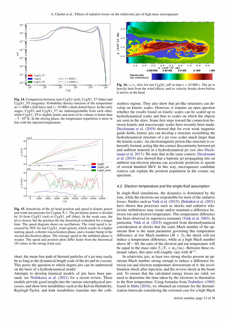
A decrease in the jet kinetic power decreases its propagation ef-ficiency as well as its stability. Starting from our fiducial testcases CygX1 and CygX3, we reduced the jet power by a factorof 10 (CygX1_mP) and 2 (CygX3_mP) via reducing the jet den-sity at constant beam speed, as detailed in Tables D.2 and D.4in the appendix. In these modified settings, the jets are expectedto propagate more slowly and to be more prone to instabilitiesbecause the inertial mass density is lower as long as the jet isnot disrupted by the stellar wind, as pointed out in Perucho et al.(2010a). This occurs for run CygX1_mP, as shown in Fig. 16.At constant beam speed vb, the amplitude of the speed variationsalong the trend defined in the beginning of this section and thetimescales at which they occur are controlled by the injected ki-netic power, but the trend itself is not affected.

Figure 15 shows propagation plots for runs CygX1 (red) andCygX1_mP (blue), with the same parameters except for ρb ,which is ten times smaller in the second case. The weak jet dis-plays a different behavior as the beam is strongly bent away bythe wind and is then broken down by instabilities after t = 8000



0 2000 4000 6000 8000 10000 12000 14000t [s]

10 15

10 12

10 9

10 6

10 3

100

103

P rad

[erg

s1 c

m3 ]

CygX1ffsynicline

ffsynicline

beaminner c.outer c.

0 1000 2000 3000 4000 5000 6000t [s]

10 11

10 9

10 7

10 5

10 3

10 1

101

103

105

P rad

[erg

s1 c

m3 ]

CygX3ffsynicline

beaminner c.outer c.

Fig. 7. Time evolution of radiative losses for the fiducial runs CygX1(top) and CygX3 (bottom), derived at each cell and summed per zone,at time steps t = (500, 2000, 4000, 6000, 10000, 15000) s for CygX1and t = (250, 500, 750, 1500, 3000, 6000) s for CygX3 (two data pointsper evolutionary phase). In both cases, free-free losses dominate coolingin the inner cocoon and beam, while line cooling dominates the outercocoon.

s, as shown in red in Fig. 16, drawn at t = 10 000 s. The beammixes with the cocoon farther away from the contact discontinu-ity, and the momentum flowing from the reverse shock at beamhead is partly dissipated in the cocoon. This smoothes the ef-fects of beam head oscillations on the jet head dynamics andalso slows the jet propagation down.

The propagation of runs CygX3 and CygX3_mP is shown inthe left panel of Fig. 17. ρb is here divided by 2 between the tworuns. In this case, the remark about the shape of the speed plotholds also: weaker jets show a similar evolution with smaller am-plitudes in the global variations of the jet velocity. In contrast tothe Cygnus X-1 case, however, a decrease in density destabilizesthe jet: the first speed peak that occurs when the jet propagationbreaks from the momentum balance model occurs earlier in theweak case, and the speed fluctuations begin earlier.

3.4.3. Wind effects on the jet propagation

An increase in the wind ram pressure shortens the instabilitygrowth phase. This shows that this deceleration and the wind

0

2

4

6

x h [c

m]

1e13

0 2500 5000 7500 10000 12500 15000 17500t [s]

2

4

6

v h [c

m/s

]1e9 CygX1

CygX1_noLossCygX1CygX1_noLoss

datamomentum bal.

Fig. 8. Effects of losses on run CygX1 structure and dynamics. Top:Temperature slices of runs CygX1 and CygX1_noLoss at time t = 15000 s. Both jets display similar structures, with the exception of aslightly larger outer cocoon at the head of the non-cooled jet. Bottom:Jet head propagation and speed of the same runs, CygX1 in red andCygX1_noLoss in blue. The theoretical 1D propagation from AppendixA.1 is drawn as dotted lines following the same color-coding. The prop-agation is identical in both runs until the start of the turbulent phase,after which speed fluctuations differ, but the average propagation speedis identical in the two runs with almost no difference in the jet headposition plot.

impact on the beam are linked. In the Cygnus X-1 runs, the im-pact of a stellar wind speed that is 50% higher and thereforecauses an increase of 50% in the wind ram pressure at a constantmass-loss rate is shown in Fig. 15 by comparing the CygX1 (red)and CygX1_wind (green) runs: the stronger the wind speed, theshorter the instability growth phase. The beginning of this phasealso starts slightly earlier: at 1800 s for CygX1_wind versus2200 s in the fiducial case. The ambient density, moreover, dropsslightly from CygX1 to CygX1_wind because M? is constantbetween the two runs. This means a higher η and therefore aneasier jet propagation through the medium, and it explains thedifference in starting propagation speed between the two runs.The theoretical 1D estimates for position and speed deviate fromthe measured values earlier in the strong wind case because themultidimensional effects are stronger. A higher wind speed in-duces a small plateau in jet speed at the very beginning of itspropagation, which cannot be modeled by our 1D theoretical es-timate.



0.0

0.5

1.0

1.5

2.0

x h [c

m]

1e13

0 1000 2000 3000 4000 5000 6000 7000 8000t [s]

2

4

6

v h [c

m/s

]

1e9 CygX3CygX3_noLossCygX3CygX3_noLoss

datamomentum bal.

Fig. 9. Effects of losses on run CygX3 structure and dynamics. Top:Temperature slices of runs CygX3 and CygX3_noLoss at time t = 9000 s. Two main differences appear: 1) The cooled beam is thinner. Itsenvelope closely follows the internal shocks structure in contrast to thenon-cooled case. 2) The cocoon of the non-cooled jet expands farther atits basis, almost wrapping around the star, whereas in the cooled case,the cocoon has almost disappeared because ambient material has cooledenough to be blown back by the wind. Bottom: Same as Fig. 8. Thecooled jet (in red) is initially faster, but leaves the smooth phase earlier,after which point it is slower on average, as seen in the propagation plot.

For the Cygnus X-3 runs, the right panel of Fig. 17 com-pares the fiducial run CygX3 (red) with run CygX3_mW (blue),in which the wind is slower. All other parameters were keptconstant, with the exception of mass-loss rate, to ensure sameη value between the runs and halving the wind ram pressureon the jet. The right panel shows the same modification usingthe weaker jet setup (runs CygX3_mP and CygX3_mPmW).In the first case, the initial accelerating phase is twice as long

0 1000 2000 3000 4000 5000t [s]

101

p ic/p

b

CygX3CygX3_noLoss

Fig. 10. Effect of radiative losses on the CygX3 beam structure. Top:Ratio of volume-averaged pressure of the inner cocoon and beam forruns CygX3 (red) and CygX3_noLoss (blue). The overpressure is al-ways higher in the cooled case. Bottom: Tracer density at t = 750 sfor runs CygX3 and CygX3_noLoss. The cooled jet features strongeroblique shocks.

for run CygX3_mW than run CygX3, and the second phasein run CygX3_mW consists only of a global deceleration be-cause no reacceleration is observable. After this deceleration, runCygX3_mW shows a slightly higher median propagation speed.

When we compare runs CygX3_mP and CygX3_mPmWin the bottom right panel of Fig. 17, a new effect arises: in-stead of a deceleration, the initial acceleration phase of runCygX3_mPmW is followed by a plateau. The velocity fluctu-ations around the trend also appear later, but with a greater am-plitude when the wind is weaker. After this speed plateau, thejet decelerates to a median value similar to the strong wind case,while the speed fluctuation timescale also decreases to a similarvalue as the strong wind case. This occurs after t ∼ 3000 s, whenthe jet has propagated to a distance of ∼ 5 · 1012 cm (= 20 dorb).At this point, the wind is almost colinear with the jet propaga-tion, and its lateral ram pressure on the jet is negligible.



102 103 104

t [s]

1032

1034

1036

1038

Volu

me

[cm

3 ]

CygX3CygX3_noLoss


Fig. 11. Volumes of the different jet zones as a function of time are af-fected differently by radiative cooling. The outer cocoon is larger with-out losses, while the volumes are comparable for the inner cocoon. Thepower-law dependence on time of the cocoon is robust for the cocoon,but not for the beam.

0

2

4

6

x h [c

m]

1e13

0 2000 4000 6000 8000 10000 12000 14000 16000t [s]

2

4

6

v h [c

m/s

]

1e9CygX1_T7CygX1CygX1_T9

CygX1_T7CygX1CygX1_T9

datamomentum bal.

Fig. 12. Jet head propagation and speed for runs CygX1_T7 (red),CygX1 (blue) and CygX1_T9. Run CygX1 slows down to the turbu-lent phase earlier than CygX1_T7, but display the same average speedduring the turbulent phase, as shown by the almost parallel propagationcurves. Run CygX1_T9 displays a different behaviour, decelerating to aplateau in the instability growth phase and with a lower average speedthan the other two runs, which appears to decelerate after t = 12 000 s.

4. Discussion

We have simulated jet outbreak and propagation in a large spatialand temporal frame based on the physical model developed inSects. 2.1 and 2.4. The simulation particularly included radiativecooling by different processes. We now critically discuss someunderlying points of this model and the limitations of the results,and we describe the directions in which future work should beoriented. This point is of peculiar importance if we wish to com-pare simulation results to observations.

0 2000 4000 6000 8000 10000 12000 14000t [s]

109

1010

T [K

]



0 2000 4000 6000 8000 10000 12000 14000t [s]

100

2 × 100

p ic/p

b


Fig. 13. Comparison of temperature and overpressure of runsCygX1_T7, CygX1 and CygX1_T9, the color-coding is the same asin Fig. 12. Top: Evolution of the zone-averaged temperature with simu-lation time. CygX1 and CygX1_T7 differ only slightly at first, but thenstart to evolve differently after the 5000 s mark. CygX1_T9 shows anoverall higher temperature, with a small peak in inner cocoon temper-ature around t=6000 s. Bottom: Evolution of the ratio of the inner co-coon to beam pressure, as defined Sect. 3.3.1. CygX1 and CygX1_T7present similar values up to t ∼ 5 000 s, while CygX1_T9 presents astronger overpressure.

4.1. Assumption of a hydrodynamical framework

High-energy nonthermal photons are a prominent feature of mi-croquasar observations. They are present in the low and highstate, but in different forms. They are thought to be producedby nonthermal processes that occur in the jet (Molina & Bosch-Ramon 2018; Poutanen & Veledina 2014; Malzac et al. 2018), inwhich high-energy particles are accelerated to relativistic speedsand adopt a power-law spectrum. The mechanisms invoked toaccelerate particles are stochastic acceleration (Fermi mecha-nism) at shocks, magnetic reconnection, or wave turbulence; seethe recent reviews by Marcowith et al. (2020); Matthews et al.(2020). All these acceleration mechanisms imperatively demandthe plasma to be collisionless to a high degree. The Coulomb-logarithm of a typical jet beam in microquasars is approximately15 and even higher in large regions of the cocoon. Consequently,kinetic timescales and kinetic inertial length scales are more than10 orders of magnitude smaller than hydrodynamical scales. In



106 107 108 109 1010 1011

T [K]

10 8

10 7

10 6

10 5

10 4

10 3

10 2

10 1

pdf


t = 4000 st = 10000 s

Fig. 14. Comparison between runs CygX1 (red), CygX1_T7 (blue) andCygX1_T9 (magenta). Probability density function of the temperatureat t = 4000 s (full lines) and t = 10 000 s (dash-dotted lines). In the earlystages, CygX1 and CygX1_T7 are indistinguishable from each other,while CygX1_T9 is slightly hotter and more of its volume is hotter than∼ 5 · 109 K. In the mixing phase, the temperature repartition is more inline with the injected temperature.

0

2

4

6

x h [c

m]

1e13

0 2000 4000 6000 8000 10000 12000 14000 16000t [s]

0

2

4

6

v h [c

m/s

]

1e9

CygX1CygX1_mPCygX1_wind

CygX1CygX1_mPCygX1_wind

datamomentum bal.

Fig. 15. Sensitivity of the jet head position and speed to kinetic powerand wind ram pressure for Cygnus X-1. The jet kinetic power is dividedby 10 from CygX1 (red) to CygX1_mP (blue). In the weak case, thejet is slower, but the position fits the theoretical evaluation for a longertime. The speed diagram shows no oscillations. The wind speed is in-creased by 50% for run CygX1_wind (green), which results in a higherstarting speed, a shorter reacceleration phase, and a weaker bump in thesecond deceleration phase. The average speed in the turbulent phase isweaker. The speed and position plots differ faster from the theoretical1D values in the strong wind case.

short, the mean free path of thermal particles of a jet may easilybe as long as the dynamical length scale of the jet and its cocoon.This poses the question to which degree jets can be understoodon the basis of a hydrodynamical model.Attempts to develop kinetical models of jets have been pur-sued; see Nishikawa et al. (2021) for a recent review. Thesemodels provide good insight into the various microphysical pro-cesses, and show how instabilities such as the Kelvin-Helmholtz,Rayleigh-Taylor, and kink instabilities translate into the colli-

Fig. 16. vx/v j slice for run CygX1_mP at time t = 10 000 s. The jet isheavily bent from the wind effects, and its velocity breaks down beforeit arrives at the head.

sionless regime. They also show that jet-like structures can de-velop on kinetic scales. However, it remains an open questionwhether the results found on kinetic scales can be scaled up tohydrodynamical scales and thus to scales on which the objectsare seen in the skies. Some first steps toward the connection be-tween kinetic and macroscopic scales have recently been made:Dieckmann et al. (2019) showed that for even weak magneticguide fields, kinetic jets can develop a structure resembling thehydrodynamical structure of a jet over scales much larger thanthe kinetic scales. An electromagnetic piston-like structure is co-herently formed, acting like the contact discontinuity between jetand ambient material in a hydrodynamical jet (see also Dieck-mann et al. 2017). We note that in the same context, Dieckmannet al. (2019) also showed that a leptonic jet propagating into anambient ion-electron plasma can accelerate positrons to speedsof several hundred MeV. In this way, microquasars candidatesources can explain the positron population in the cosmic rayspectrum.

4.2. Electron temperature and the single-fluid assumption

In single-fluid simulations, the dynamics is dominated by theions, while the electrons are responsible for most of the radiativelosses. Studies such as Vink et al. (2015); Zhdankin et al. (2021)have shown that processes such as shocks and radiative rela-tivistic turbulences may create and/or maintain a difference be-tween ion and electron temperature. This temperature differencehas been observed in supernova remnants (Vink et al. 2003). Inparticular, Vink et al. (2015) suggested from thermodynamicalconsideration at shocks that the sonic Mach number of the up-stream flow is the main parameter governing this temperaturedifference: at low Mach numbers (M ≤ 2), the shock will notinduce a temperature difference, while at a high Mach numberabove M ∼ 60, the ratio of the electron and ion temperature willbe equal to the mass ratio Te/Ti = me/〈mi〉. Between these ex-tremal values, this ratio will roughly vary with M−2.

In relativistic jets, at least two strong shocks present an up-stream Mach number strong enough to induce a difference be-tween ion and electron temperature downstream of it: the recol-limation shock after injection, and the reverse shock at the beamend. To ensure that the calculated energy losses are valid, weneed to determine the time taken by the electrons to thermalizeto the flow temperature. Using formulas from Trubnikov (1965)found in Huba (2016), we obtained an estimate for the thermal-ization timescale considering the extremal case for a high Mach



0.0

0.5

1.0

1.5

2.0

x h [c

m]

1e13

0 2000 4000 6000 8000t [s]

2

0

2

4

v h [c

m/s

]

1e9

CygX3CygX3_mPdatamomentum bal.

0.0

0.5

1.0

1.5

2.0

2.5

x h [c

m]

1e13

0 1000 2000 3000 4000 5000 6000 7000 8000t [s]

0

2

4

6

8

v h [c

m/s

]

1e9CygX3CygX3_mWdatamomentum bal.

0.00

0.25

0.50

0.75

1.00

x h [c

m]

1e13

0 2000 4000 6000 8000t [s]

2

0

2

4

v h [c

m/s

]

1e9CygX3_mPCygX3_mPmWdatamomentum bal.

Fig. 17. Sensitivity of the jet head position and speed to kinetic power (left) and wind momentum (right) for the Cygnus X-3 runs. Top left: Adivision of the jet power by 2 decreases all dynamical values, starting from the mean propagation speed. In particular, the acceleration is far lessefficient: it shows a gain of ∼ 40% in speed between the starting point and the peak against a gain of ∼ 120% in the CygX3 run. Top right: Areduction of M? by 25% and vw by 33% (keeping η constant) lengthens the smooth phase and strengthens the speed fluctuations in the followingphases. The jets settle to the same median speed in the turbulent phase. Bottom right: Same reduction as in the top right panel, with half the jetpower. In the CygX3_mPmW case (right, blue), the initial acceleration phase is followed by a speed plateau.

number. Table 3 presents the rest mass density and temperaturevalues after the recollimation shock and reverse shock in CygX1at t = 5000 s and CygX3 at t = 1000 s, the derived thermaliza-tion timescale, and the associated characteristic length using thelocal flow speed value. In all cases except downstream of theCygX3 reverse shock, the associated length scale is shorter thanthe grid resolution, meaning that the electrons would have ther-malized to the flow temperature after a single simulation griddownstream of the shock. In the last case, we can estimate thevolume whithin which an error is made using the flow tempera-ture to derive losses as Vtherm = vhc2

s t3therm, where cs is the local

sound speed. With vh = 3 · 109 cm s−1 at t = 1000 s, we obtainVtherm = 3.3 · 1033 cm3, which accounts for 0.37% of the innercocoon volume at that time. We then consider our Te = Ti = Tapproximation to be valid in our hydrodynamical framework. Ina more realistic framework in which the plasma is collisionless(see the discussion in Sect. 4.1), Coulomb interactions cannotequilibrate the electron and ion temperatures, but other processessuch as plasma instabilities may fill that role.

shock ρ (g cm)−3 T (K) ttherm (s) ltherm (cm)X1 recoll. 5 · 10−15 5 · 108 4.2 · 10−4 4 · 106

X1 reverse 10−15 3 · 1010 0.6 2 · 109

X3 recoll. 10−14 4 · 1010 0.1 2.25 · 109

X3 reverse 5 · 10−15 1012 19 2 · 1011

Table 3. Thermalization of electrons downstream of a shock.

4.3. Thermal diffusion

Another important process that in not included in our numericalmodel is thermal diffusion by relativistic thermal and nonther-mal electrons or X-ray photons. This process is likely importantas it creates hot shock-precursors, decreases peak temperatures,smoothes out contact interfaces, and enhances cooling. Thesefeatures are suggested when looking at work which includes theprocess in the context of supernova remnants (Chevalier 1975;Tilley et al. 2006) and colliding winds in binary systems (Myas-nikov & Zhekov 1998; Motamen et al. 1999). Including heat



transfer in a simulation is numerically demanding as it demands(semi-) implicite solvers due to the very stiffness of the pro-cess. Nevertheless, a few attempts have been made to developperforming solvers (Balsara et al. 2008; Palenzuela et al. 2009;Viallet et al. 2011; Kupka et al. 2012; Commerçon et al. 2014;Bucciantini & Del Zanna 2013; Dubois & Commerçon 2016;Viallet et al. 2016). Future work may expand these attempts tojet simulations.

4.4. Wind structure and jet bending

In high-mass microquasars, jets are launched into winds origi-nating from orbiting and rotating stars. This causes a circumbi-nary environment structured in Archimedean spirals in colliding-wind binaries (Walder 1995) and accreting binaries (Walder et al.2008, 2014). These spirals, also called corotating interaction re-gions (CIRs), are bound by shocks that confine high-density,high-temperature regions. These structures will likely have animpact on the jet propagation and its stability, but will also likelylead to flashing outbursts in emission.

The bending of the jet away from the mass-shedding donorstar, investigated, for example, by Perucho & Bosch-Ramon(2008) and subsequent papers, Yoon & Heinz (2015), Bosch-Ramon & Barkov (2016), and again confirmed in this paper, willlead to helical jet trajectories. In the most extreme cases, an ob-server will see the jet under different angles during an orbit of thesystem (see, e.g., Horton et al. 2020). Future works will lead to amore quantitative statement of this prediction. As a side note, weshowed in Sect. C.4 that jets performed with a relativistic schemedisplay a higher propagation speed, even in the mildly relativis-tic case. Because the jet bending depends on the transverse mo-mentum accumulated by the jet during its propagation, we wouldexpect a weaker bending in relativistic simulations than in New-tonian simulations that are performed with the same parameters.

Another unknown is wind clumping. We know that windsfrom hot massive stars are clumped (e.g., Oskinova et al. 2012),with density contrasts 〈ρ2〉/〈ρ〉2 ≈ 2. Poutanen et al. (2008) sug-gested that this is likely the case for Cygnus X-1 based on dips inthe X-ray light curve (Bałucinska-Church et al. 2000; Miskovi-cová, Ivica et al. 2016; ?). It is unknown, however, where theseclumps are formed: in the stellar atmosphere, or farther awayfrom the star, for instance, by supersonic turbulence in the wind.Whether these clumps are small and dense, an intermittent den-sity fluctuation of compressible turbulence, or a mix of both isunknown as well; see the discussion in Walder & Folini (2003).Perucho & Bosch-Ramon (2012) suggested that even moderatewind clumping has strong effects on jet disruption, mass loading,bending, and likely energy dissipation. de la Cita et al. (2017)suggested that the standing shocks introduced in the jet flow byits interaction with a clumpy wind would generate a higher ap-parent gamma-ray luminosity through inverse Compton scatter-ing of the stellar photons, as well as efficient synchrotron cool-ing. In light of these results, we may expect that introducingclumpiness in the wind might significantly enhance the radiativecooling of the jet and modify its dynamics even more strongly.

4.5. Wind driving and dynamics

Velocity and density profiles in winds shed from hot massivestars in binaries are prone to a large uncertainty. This uncertaintypushed us to choose a grid of fixed wind parameters for the studypresented in this paper and to make no attempts to model theacceleration of the wind. Winds from massive stars are driven

by the radiative pressure on free electrons (to about one-third ofthe driving force) as well as the scattering of stellar photons inmillions of UV and optical lines. This wind driving is expectedto be vastly different in supergiants (as in Cygnus X-1) and WRstars (as in Cygnus X-3), in that the winds from WR stars areoptically thick in the subsonic acceleration phase, whereas theyare relatively optically thin in supergiant winds.

These winds are well understood for single stars, with theexception of the subsonic phase of WR winds; see the reviewby Kudritzki & Puls (2000). In binaries, the situation is morecomplex. Hainich et al. (2020) presented an observation-basedstudy of winds in HMXRBs and basically confirmed that thewind driving from stars in those binaries is the same as for sin-gle stars of the same type. However, the situation is more com-plicated by the secondary radiation source, either another star ora compact object and its environment. This second source leadsto an ionization structure within the wind that in contrast to thesingle-star situation does not fit the frequencies of the photonsemitted by the star that produces the wind.

This in particular affects the region between the wind-shedding star and its companion. There, the driving by photonscattering in spectral lines can be suppressed and the wind accel-eration may be weaker or even inhibited compared to the windsof a single star (Stevens & Kallman 1990; Stevens 1991; Blondin1994). Models that take this inhibition into account can be fit toobservations (Gies et al. 2008). The case of Cygnus X-1 wasinvestigated through complex radiation hydrodynamics simula-tions by Hadrava & Cechura (2012) and Krticka et al. (2015),who suggested that strong inhibition of the wind speed mightoccur at the BH location. In this region, wind density and veloc-ity profiles in binaries are very difficult to access observationallyand are largely unknown. For Cygnus X-3, the situation is evenmore unknown because the wind is still optically thick at the BHlocation. Studies such as those by Vilhu et al. (2021) find a strongwind-suppressing effect in particular in the extreme-UV region.However, we can firmly state that a wind is present in both sys-tems, based on the modulation of the X-ray light curve over thebinary orbit, for instance. This modulation is due to the differentoptical paths that X-ray photons have to travel through the windand thus to the different attenuation of the X-ray light throughabsorption in the wind (Bonnet-Bidaud & van der Klis 1981;Poutanen et al. 2008; ?). Finally, the effect of the BH gravita-tional field must be considered, which may focus the stellar windand modify the density and velocity profile that are encounteredby the propagating jet, but might also modify the evolution ofthe jet cocoon at its base.

Another important open problem is the influence of magneticfields on the wind because strong fields could substantially in-fluence the mass-shedding process, for example, by a strong en-hancement of the mass loss in the equatorial plane (ud-Doulaet al. 2006; Ud-Doula et al. 2008; Bard & Townsend 2016). Ageneral discussion of magnetic fields of massive stars and howthey influence their environment can be found in Walder et al.(2012).

4.6. Nonthermal components and radiative processesemission

Our losses are modeled as optically thin at every frequencies.This may not be the case, especially in UV, optical, and radioranges at which our thermal electrons radiates. Reheating dueto photon absorption (Belmont et al. 2008) or synchrotron self-absorption as well as effects such as synchrotron self-Compton



were not investigated and may have a strong impact on the jettemperature and therefore structure and dynamics. This may nothold for Cygnus X-1, for which cooling and its effects are mod-erate but it might play a strong role in Cygnus X-3 case, es-pecially because winds from WR stars are optically thick overhigher frequency bands than winds from O-type stars. Moreover,the temperatures attained in our simulations exceed the electronpair-production threshold and reach a regime in which protondistribution becomes relativistic, which will impact the radiativelosses.

Another point we did not consider is the particle accelera-tion and the nonthermal processes: particles can be acceleratedat magnetic reconnections (Giannios 2010; Giannios et al. 2009;McKinney & Uzdensky 2012; Melzani et al. 2014) and shocks(Araudo et al. 2009; Bordas et al. 2009; de la Cita et al. 2017) orby stochastic interaction with magnetized turbulence. Shearingflow acceleration as also been invoked as potential injection pro-cess of relativistic particles (Rieger & Duffy 2019). An extensivereview of these processes is given in Marcowith et al. (2020).As all processes will significantly contribute to the nonthermalemission, they can inject a substantial fraction of the kinetic jetenergy into nonthermal components and probably change thedynamics because part of the gas energy will be dissipated bythe accelerated particles. Alternatively, the pressure imparted tothese particles can directly modify the flow dynamics.

4.7. Jet outburst dynamics and emerging structures

The dynamics of the second (instability) phase is not well un-derstood, and neither is the physical phenomenon that sets thefluctuation speeds. The physics of instability growth is deepand rich, and we may have overlooked some effects, in partic-ular, concerning the nonlinear phase. Another limitation of thisstudy is our grid resolution, which may not accurately captureall the shocks that form in such a system or the growth of small-amplitude modes, for which the impact was highlighted here.Furthermoer, the adiabatic index Γ was chosen to be constantand equal to 5/3, where a variable index such as the methodsuggested in Mignone et al. (2005) and Mignone & McKin-ney (2007) would more accurately reflect the relativistic gas EoS(Synge 1957) and lead to more realistic jet structures.

We included thermal radiative losses in our study of jetsstructure and dynamics. These effects were not included in sim-ilar works. No focus was placed on jet bending, but it is observ-able in the jets of Cygnus X-1 and Cygnus X-3, in agreementwith similar studies such as Yoon & Heinz (2015). Moreover, thejets are injected with no inclination relative to the orbital plane,in contrast to works such as Dubus et al. (2010), who suggestedthat the inclination angle for Cygnus X-3 lies between 20 and80◦. Another strong point of this study is the simulation box sizeof 1014 cm, which is 33 times the orbital separation of CygnusX-1 and close to 400 times that of Cygnus X-3. This allowedus to observe the outbreak and early dynamics details as wellas the emergence of a steady "naked beam" structure for latertimesteps that may be compared to similar works and translatedinto synthetic observational datas.

Last, our study is purely hydrodynamical and does not coverthe potential stabilizing effects of the magnetic field as well asthe development of MHD instabilities. The study of MHD jetsis recent (e.g. Mizuno et al. 2015; Martí et al. 2016; Mukherjeeet al. 2020) and the field will continue to grow as time passes.The influence of the stellar magnetic field may also lead to fur-ther modifications on the structure and dynamics of the jet.

5. Summary and conclusions

We performed large-scale 3D relativistic hydrodynamical sim-ulations of jet outbreak and early propagation in HMMQs. Weadded radiative cooling effects in the energy equation usinga Maxwell-Jüttner distribution for the electrons. Two fiducialcases inspired by the HMMQs Cygnus X-1 and Cygnus X-3were considered, along with parameter sensitivity studies. Thejets of the two systems are in the same domain of dimension-less parameters, but with different instability growth and coolingtimescales (about ∼ 102 shorter in the latter case), enabling us tobetter highlight the importance of these processes in jet structureand dynamics. In particular, on the timescales covered by oursimulations, radiative losses, mainly free-free mechanism, playa relevant role for Cygnus X-3, but not for Cygnus X-1.

We investigated the impact of radiative losses on jet struc-tures and dynamics and showed their strengthening effect onKHI growth, which was a focal point of our analysis. We identi-fied three main dynamical phases: 1) an initial self-similar prop-agation in line with 1D momentum balance arguments, followedby 2) a modification of the inner jet structure and a phase ofinstability growth, and finally, 3) a turbulent cocoon and destabi-lized beam. We explored the effects of losses on the dynamics inthe second phase through their modification of the KHI growthrate as well as the impact on the jet structure, and we examinedthe impact of the various parameters.

In Cygnus X-3, where radiative losses are observed on thetimescales covered by our simulations, these losses are found toaffect the volume ratio of the outer to inner cocoon. This meansthat simple postprocessing of simulations that do not take radia-tive cooling into account to study emissions from HMMQ jetsmust be met with caution. Likewise, the beam volume is foundto obey a different power law in time depending on whether ornot cooling is active.

We find the sensitivities to jet power and wind parameters tobe in line with the literature. We add to this picture by demon-strating that an increasing beam temperature results in a fasterinstability growth and a slower jet head velocity. In view of thewide variety of known HMMQs, but also given the difficult es-timation of their system parameters, further and more extendedparameter studies are clearly desirable in the future. Based onthe results presented here, we would advocate that such studiesnot be limited to adiabatic simulations.Acknowledgements. We acknowledge support from the French National Pro-gram for High Energies (PNHE). Simulations have been performed at the PôleScientifique de Modélisation Numérique (PSMN) hosted by the ENS de Lyon,and at the centers of the Grand Equipement National de Calcul Intensif (GENCI)under grant number A0090406960. We thank the referee for the helpful reviewand insights, which helped improve the paper significantly.

ReferencesAlbert, A., Alfaro, R., Alvarez, C., et al. 2021, ApJ, 912, L4Allen, A. & Hughes, P. 1984, MNRAS, 208, 609Araudo, A. T., Bosch-Ramon, V., & Romero, G. E. 2009, A&A, 503, 673Balsara, D. S., Tilley, D. A., & Howk, J. C. 2008, MNRAS, 386, 627Bałucinska-Church, M., Church, M. J., Charles, P. A., et al. 2000, MNRAS, 311,

861Bard, C. & Townsend, R. H. D. 2016, MNRAS, 462, 3672Belmont, R., Malzac, J., & Marcowith, A. 2008, A&A, 491, 617Bertschinger, E. 1986, ApJ, 304, 154Blandford, R. & Pringle, J. 1976, MNRAS, 176, 443Blandford, R. D. & Payne, D. G. 1982, MNRAS, 199, 883Blandford, R. D. & Znajek, R. L. 1977, MNRAS, 179, 433Blondin, J. M. 1994, ApJ, 435, 756Bodo, G., Massaglia, S., Ferrari, A., & Trussoni, E. 1994, A&A, 283, 655Bodo, G. & Tavecchio, F. 2018, A&A, 609, A122



Bonnet-Bidaud, J. M. & van der Klis, M. 1981, A&A, 101, 299Bordas, P., Bosch-Ramon, V., Paredes, J. M., & Perucho, M. 2009, A&A, 497,

325Boris, J. P., Grinstein, F. F., Oran, E. S., & Kolbe, R. L. 1992, Fluid Dynamics

Research, 10, 199Bosch-Ramon, V. & Barkov, M. 2016, A&A, 590, A119Brent, R. 1973, Algorithms for Minimization without Derivatives, Prentice-Hall,

Englewood Cliffs, NJBucciantini, N. & Del Zanna, L. 2013, MNRAS, 428, 71Chevalier, R. A. 1975, ApJ, 198, 355Chevalier, R. A. & Imamura, J. N. 1982, ApJ, 261, 543Commerçon, B., Debout, V., & Teyssier, R. 2014, A&A, 563, A11Cook, J., Cheng, C.-C., Jacobs, V., & Antiochos, S. 1989, APJ, 338, 1176de la Cita, V. M., del Palacio, S., Bosch-Ramon, V., et al. 2017, A&A, 604, A39Del Zanna, L. & Bucciantini, N. 2002, A&A, 390, 1177Del Zanna, L., Zanotti, O., Bucciantini, N., & Londrillo, P. 2007, A&A, 473, 11Dieckmann, M. E., Folini, D., Hotz, I., et al. 2019, A&A, 621, A142Dieckmann, M. E., Folini, D., Walder, R., et al. 2017, Physics of Plasmas, 24,

094502Donat, R., Font, J. A., Ibáñez, J. M. S. S., & Marquina, A. 1998, Journal of

Computational Physics, 146, 58Dubois, Y. & Commerçon, B. 2016, A&A, 585, A138Dubus, G., Cerutti, B., & Henri, G. 2010, MNRAS: Letters, 404, L55Duffell, P. C. & MacFadyen, A. I. 2011, APJ Supplement Series, 197, 15Ferrari, A., Massaglia, S., & Trussoni, E. 1982, Monthly Notices of the Royal

Astronomical Society, 198, 1065Ferrari, A., Trussoni, E., & Zaninetti, L. 1978, A&A, 64, 43Folini, D., Heyvaerts, J., & Walder, R. 2004, A&A, 414, 559Folini, D. & Walder, R. 2006, A&A, 459, 1Folini, D., Walder, R., & Favre, J. M. 2014, A&A, 562, A112Folini, D., Walder, R., Psarros, M., & Desboeufs, A. 2003, in Stellar Atmosphere

Modeling, Vol. 288, 433Gallo, E., Fender, R., Kaiser, C., et al. 2005, Nature, 436, 819Garnier, E., Mossi, M., Sagaut, P., Comte, P., & Deville, M. 1999, Journal of

Computational Physics, 153, 273Ghisellini, G. 2013, Radiative processes in high energy astrophysics, Vol. 873

(Springer)Ghisellini, G. & Tavecchio, F. 2010, MNRAS: Letters, 409, L79Giannios, D. 2010, MNRAS, 408, L46Giannios, D., Uzdensky, D. A., & Begelman, M. C. 2009, MNRAS, 395, L29Gies, D. R., Bolton, C. T., Blake, R. M., et al. 2008, ApJ, 678, 1237Gómez, J., Martí, J. M., Marscher, A., Ibáñez, J. M., & Alberdi, A. 1997, APJ

Letters, 482, L33Gómez, J., Martí, J. M., Marscher, A., Ibáñez, J. M., & Marcaide, J. 1995, APJ

Letters, 449, L19Gottlieb, S., Shu, C.-W., & Tadmor, E. 2001, SIAM Review, 43, 89Gourgouliatos, K. N. & Komissarov, S. S. 2018, Nature Astronomy, 2, 167Gourgouliatos, K. N. & Komissarov, S. S. 2018, MNRAS: letters, 475, L125Grinberg, V., Leutenegger, M. A., Hell, N., et al. 2015, A&A, 576, A117Hadrava, P. & Cechura, J. 2012, A&A, 542, A42Hainich, R., Oskinova, L. M., Torrejón, J. M., et al. 2020, A&A, 634, A49Hanasz, M. & Sol, H. 1996, A&A, 315, 355Hanasz, M. & Sol, H. 1998, A&A, 339, 629Hardee, P. 1979, APJ, 234, 47Hardee, P. E., Hughes, P. A., Rosen, A., & Gomez, E. A. 2001, APJ, 555, 744Hardee, P. E., Rosen, A., Hughes, P. A., & Duncan, G. C. 1998, APJ, 500, 599Hirsch, C. 2006, Numerical Computation of Internal and External Flows

(Butterworth-Heinemann Limited)Hirsch, M., Hell, N., Grinberg, V., et al. 2019, A&A, 626, A64Horton, M. A., Krause, M. G. H., & Hardcastle, M. J. 2020, MNRAS, 499, 5765Huba, J. D. 2016, NRL plasma formulary (Naval Research Laboratory)Jüttner, F. 1911, Annalen der Physik, 339, 856Komissarov, S. S., Porth, O., & Lyutikov, M. 2015, Computational astrophysics

and cosmology, 2, 1Krticka, J., Kubát, J., & Krticková, I. 2015, A&A, 579, A111Kudritzki, R.-P. & Puls, J. 2000, ARA&A, 38, 613Kupka, F., Happenhofer, N., Higueras, I., & Koch, O. 2012, Journal of Compu-

tational Physics, 231, 3561Landau, L. & Lifshitz, E. 1959, Fluid Mechanics, by L.D. Landau and E.M.

Lifshitz, Course of Theoretical Physics (Pergamon Press)LeVeque, R., Ablowitz, M., Davis, S., et al. 2002, Finite Volume Methods for

Hyperbolic Problems, Cambridge Texts in Applied Mathematics (CambridgeUniversity Press)

Malzac, J. 2014, MNRAS, 443, 299Malzac, J., Kalamkar, M., Vincentelli, F., et al. 2018, MNRAS, 480, 2054Marcowith, A., Ferrand, G., Grech, M., et al. 2020, Living Reviews in Compu-

tational Astrophysics, 6, 1Martí, J. M., Müller, E., Font, J., Ibáñez, J. M. Z., & Marquina, A. 1997, APJ,

479, 151Martí, J. M., Perucho, M., & Gómez, J. L. 2016, APJ, 831, 163

Matsumoto, J., Aloy, M. A., & Perucho, M. 2017, MNRAS, 472, 1421Matsumoto, J. & Masada, Y. 2013, APJ Letters, 772, L1Matsumoto, J. & Masada, Y. 2019, MNRAS, 490, 4271Matthews, J. H., Bell, A. R., & Blundell, K. M. 2020, New A Rev., 89, 101543McKinney, J. C. & Uzdensky, D. A. 2012, MNRAS, 419, 573Meliani, Z. & Keppens, R. 2007, A&A, 475, 785Meliani, Z. & Keppens, R. 2009, APJ, 705, 1594Melzani, M., Walder, R., Folini, D., Winisdoerffer, C., & Favre, J. M. 2014,

A&A, 570, A112Melzani, M., Winisdoerffer, C., Walder, R., et al. 2013, A&A, 558, A133Migliori, G., Corbel, S., Tomsick, J. A., et al. 2017, MNRAS, 472, 141Mignone, A. & McKinney, J. C. 2007, MNRAS, 378, 1118Mignone, A., Plewa, T., & Bodo, G. 2005, APJ Supplement Series, 160, 199Mihalas, D. & Mihalas, B. W. 2013, Foundations of radiation hydrodynamics

(Courier Corporation)Millas, D., Keppens, R., & Meliani, Z. 2017, MNRAS, 470, 592Mirabel, I. F. & Rodriguez, L. F. 1999, Annual Review of Astronomy and Astro-

physics, 37, 409Miskovicová, Ivica, Hell, Natalie, Hanke, Manfred, et al. 2016, A&A, 590, A114Mizuno, Y., Gomez, J. L., Nishikawa, K.-I., et al. 2015, APJ, 809, 38Mizuno, Y., Hardee, P., & Nishikawa, K.-I. 2007, APJ, 662, 835Mizuta, A., Yamada, S., & Takabe, H. 2004, APJ, 606, 804Molina, E. & Bosch-Ramon, V. 2018, A&A, 618, A146Molina, E., del Palacio, S., & Bosch-Ramon, V. 2019, A&A, 629, A129Moreau, J.-P. 2005, Numerical Analysis by Jean-Pierre Moreau, http://jean-pierre.moreau.pagesperso-orange.fr

Motamen, S. M., Walder, R., & Folini, D. 1999, in Wolf-Rayet Phenomena inMassive Stars and Starburst Galaxies, ed. K. A. van der Hucht, G. Koenigs-berger, & P. R. J. Eenens, Vol. 193, 378

Motta, S. E., Rodriguez, J., Jourdain, E., et al. 2021, New A Rev., 93, 101618Mukherjee, D., Bodo, G., Mignone, A., Rossi, P., & Vaidya, B. 2020, MNRAS,

499, 681Myasnikov, A. V. & Zhekov, S. A. 1998, MNRAS, 300, 686Nishihara, K., Wouchuk, J., Matsuoka, C., Ishizaki, R., & Zhakhovsky, V. 2010,

Philosophical Transactions of the Royal Society A: Mathematical, Physicaland Engineering Sciences, 368, 1769

Nishikawa, K., DuÅ£an, I., Köhn, C., & Mizuno, Y. 2021, Living Reviews inComputational Astrophysics, 7, 1

Norman, M. L., Winkler, K.-H., Smarr, L., & Smith, M. 1982, A&A, 113, 285Orosz, J. A., McClintock, J. E., Aufdenberg, J. P., et al. 2011, APJ, 742, 84Oskinova, L. M., Feldmeier, A., & Kretschmar, P. 2012, MNRAS, 421, 2820Palenzuela, C., Lehner, L., Reula, O., & Rezzolla, L. 2009, MNRAS, 394, 1727Perucho, M. 2019, in High Energy Phenomena in Relativistic Outflows VII, 99Perucho, M. & Bosch-Ramon, V. 2008, A&A, 482, 917Perucho, M. & Bosch-Ramon, V. 2012, A&A, 539, A57Perucho, M., Bosch-Ramon, V., & Khangulyan, D. 2010a, A&A, 512, L4Perucho, M., Bosch-Ramon, V., & Khangulyan, D. 2010b, International Journal

of Modern Physics D, 19, 791Perucho, M., Hanasz, M., Marti, J.-M., & Sol, H. 2004a, A&A, 427, 415Perucho, M., Marti, J.-M., Cela, J., et al. 2010c, A&A, 519, A41Perucho, M., Marti, J.-M., & Hanasz, M. 2004b, A&A, 427, 431Perucho, M., Marti, J.-M., & Hanasz, M. 2005, A&A, 443, 863Popov, M. V., Walder, R., Folini, D., et al. 2019, A&A, 630, A129Porter, D. H., Pouquet, A., & Woodward, P. R. 1992, Theoretical and Computa-

tional Fluid Dynamics, 4, 13Porter, D. H. & Woodward, P. R. 1994, ApJS, 93, 309Poutanen, J. & Veledina, A. 2014, Space Sci. Rev., 183, 61Poutanen, J., Zdziarski, A. A., & Ibragimov, A. 2008, MNRAS, 389, 1427Rieger, F. M. & Duffy, P. 2019, ApJ, 886, L26Rodriguez, J., Grinberg, V., Laurent, P., et al. 2015, APJ, 807, 17Romero, G. E., Boettcher, M., Markoff, S., & Tavecchio, F. 2017,

Space Sci. Rev., 207, 5Rossi, P., Mignone, A., Bodo, G., Massaglia, S., & Ferrari, A. 2008, A&A, 488,

795Rybicki, G. B. & Lightman, A. P. 2008, Radiative processes in astrophysics (John

Wiley & Sons)Scheck, L., Aloy, M., Martí, J., Gómez, J., & Müller, E. 2002, MNRAS, 331,

615Shu, C.-W. & Osher, S. 1988, Journal of Computational Physics, 77, 439Stevens, I. R. 1991, ApJ, 379, 310Stevens, I. R. & Kallman, T. R. 1990, ApJ, 365, 321Synge, J. 1957, Comp. AmsterdamTilley, D. A., Balsara, D. S., & Howk, J. C. 2006, MNRAS, 371, 1106Toma, K., Komissarov, S. S., & Porth, O. 2017, MNRAS, 472, 1253Tóth, G. & Odstrcil, D. 1996, Journal of Computational Physics, 128, 82Trubnikov, B. A. 1965, Reviews of Plasma Physics, 1, 105Turland, B. & Scheuer, P. 1976, MNRAS, 176, 421Ud-Doula, A., Owocki, S. P., & Townsend, R. H. D. 2008, MNRAS, 385, 97ud-Doula, A., Townsend, R. H. D., & Owocki, S. P. 2006, ApJ, 640, L191


http://jean-pierre.moreau.pagesperso-orange.fr

http://jean-pierre.moreau.pagesperso-orange.fr


van der Holst, B., Keppens, R., & Meliani, Z. 2008, Computer Physics Commu-nications, 179, 617

van Hoof, P., Ferland, G. J., Williams, R., et al. 2015, MNRAS, 449, 2112Viallet, M., Baraffe, I., & Walder, R. 2011, A&A, 531, A86Viallet, M., Goffrey, T., Baraffe, I., et al. 2016, A&A, 586, A153Vilhu, O., Kallman, T. R., Koljonen, K., & Hannikainen, D. C. 2021, A&A, 649,

A176Vink, J., Broersen, S., Bykov, A., & Gabici, S. 2015, A&A, 579, A13Vink, J., Laming, J. M., Gu, M. F., Rasmussen, A., & Kaastra, J. S. 2003, APJL,

587, L31Walder, R. 1995, in Wolf-Rayet Stars: Binaries; Colliding Winds; Evolution, ed.

K. A. van der Hucht & P. M. Williams, Vol. 163, 420Walder, R. & Folini, D. 1996, A&AWalder, R. & Folini, D. 1998, A&A, 330, L21Walder, R. & Folini, D. 2000, in Thermal and Ionization Aspects of Flows from

Hot Stars, Vol. 204, 281Walder, R. & Folini, D. 2003, in A Massive Star Odyssey: From Main Sequence

to Supernova, ed. K. van der Hucht, A. Herrero, & C. Esteban, Vol. 212, 139Walder, R., Folini, D., & Meynet, G. 2012, Space Sci. Rev., 166, 145Walder, R., Folini, D., & Shore, S. N. 2008, A&A, 484, L9Walder, R., Melzani, M., Folini, D., Winisdoerffer, C., & Favre, J. M. 2014, in

Astronomical Society of the Pacific Conference Series, Vol. 488, 8th Inter-national Conference of Numerical Modeling of Space Plasma Flows (AS-TRONUM 2013), ed. N. V. Pogorelov, E. Audit, & G. P. Zank, 141

Wardzinski, G. & Zdziarski, A. A. 2000, MNRAS, 314, 183Wilson, M. 1987, MNRAS, 226, 447Yoon, D. & Heinz, S. 2015, APJ, 801, 55Yoon, D., Zdziarski, A. A., & Heinz, S. 2016, MNRAS, 456, 3638Zdziarski, A. A., Mikołajewska, J., & Belczynski, K. 2013, MNRAS: Letters,

429, L104Zdziarski, A. A., Pjanka, P., Sikora, M., & Stawarz, L. 2014, MNRAS, 442,

3243–3255Zhdankin, V., Uzdensky, D. A., & Kunz, M. W. 2021, APJ, 908, 71



Appendix A: Propagation and instabilities

Appendix A.1: Model for jet propagation

A model for the propagation of a relativistic jet was derived, forinstance, by Martí et al. (1997) and Mizuta et al. (2004), whoneglected multidimensional effects, but assumed 1D momentumbalance between the beam and the ambient gas in the rest frameof the contact discontinuity at the head of the jet. In the case ofan ambient medium with its own (nonrelativistic) flow speed vw, this gives

S b

[ρbhbγ

2hγ

2b(vb − vh)2 + pb

]= S w

[ρwhwγ

2h(vw − vh)2 + pw

],

(A.1)

where γ are Lorentz factors, S are cross-section areas, and v arevelocities. Subscripts b refer to beam values, w refers to the am-bient medium, and h to the interface at jet head. Solving Eq. A.1for vh, we obtain

vh =1

Aη∗ − 1

√Aη∗(vb − vw)2 − (Aη∗ − 1)

(AK − 1)c2s,w

γ2hΓ

, (A.2)

where η∗ ≡ ρbhbγ2b/ρwhwγ

2w = ξb/ξw, A is the cross-section ra-

tio (A ≡ S b/S w), and K is the pressure ratio defined in Sect.3.1. This equation is consistent with the one derived by Mizutaet al. (2004) when taking vw = 0. The term including K can beneglected as the sound speed in the stellar wind is much slowerthan the beam velocity. Assuming A = 1, Eq. A.2 therefore be-comes

vh =η∗vb − vw −

√η∗(vb − vw)

η∗ − 1. (A.3)

Appendix A.2: Instabilities in relativistic jet flows

During the jet propagation, various hydrodynamical instabilitiescan be triggered and in the end perturb the beam, reducing theeffective beam speed at the front shock and decelerating the jet.One of them is the KHI at the relativistic flow interface, whichwas extensively studied: Turland & Scheuer (1976), Blandford &Pringle (1976), Ferrari et al. (1978), Hardee (1979), Bodo et al.(1994), Hanasz & Sol (1998), Hardee et al. (1998), Hardee et al.(2001), Perucho et al. (2004a), Perucho et al. (2004b), Peruchoet al. (2005), Mizuno et al. (2007), Rossi et al. (2008), Peruchoet al. (2010c).

Then, the Rayleigh-Taylor instability (RTI) can be triggeredwhen a lighter fluid supports a heavier one against gravity, orequivalently, if the lighter fluid accelerates the heavier one (seeNorman et al. (1982), Allen & Hughes (1984), Duffell & Mac-Fadyen (2011) for nonrelativistic flows and Matsumoto et al.(2017) for relativistic flows). This impacts the jet structures sta-bility when the jet expands radially due to the centrifugal force,as studied by Meliani & Keppens (2007), Meliani & Keppens(2009), Millas et al. (2017), for example, or oscillates radi-ally because of a pressure gradient, see Matsumoto & Masada(2013), Toma et al. (2017).

Other instabilities include the Richtmyer-Meshkov instabil-ity (RMI); see Nishihara et al. (2010) for a review and Mat-sumoto & Masada (2013) for a numerical study. The centrifu-gal instability (CFI) was studied in Gourgouliatos & Komissarov(2018). Finally, we cite vortex formation and shedding at thecontact discontinuity of jet head, as in Norman et al. (1982),Scheck et al. (2002), or Mizuta et al. (2004), for instance, which

increases the cross-section of the jet head. This therefore dimin-ishes the jet propagation speed. The vortices may also perturb thebeam flow when they encounter it while propagating in the innercocoon. Norman et al. (1982) noted the importance of the beamMach number in the vortex-shedding phenomenon, observingthat lower Mach numbers produce higher vortices. This workwill focus specifically on the KHI as other instabilities developat the beam radius scale, meaning that most of their modes willnot appear due to grid resolution limitations.

Appendix A.2.1: Kelvin-Helmholtz instability

To numerically derive the linear growth time of the Kelvin-Helmholtz instability tKHI , we chose to use the approach intro-duced in Hanasz & Sol (1996), describing the jet with a 2D slabgeometry. This choice was made because the solutions for theslab and cylindrical geometries behave in a similar way in awide range of physical parameters, with only slight numericaldifferences (Ferrari et al. 1982). In this analogy, symmetric andantisymmetric modes in the slab correspond to pinching and he-lical modes in the cylinder. Only high-order fluting modes do nothave counterparts in slab jets.

Hanasz & Sol (1996) considered a core-sheet jet made ofthree layers: a beam with a relativistic flow, a cocoon with anonrelativistic flow speed, and an ambient medium at rest. Thetransition layers at all interfaces are described in the vortex-sheetapproximation. In the following, quantities with subscript b referto the beam, subscript c refers to the cocoon, and w refers to theambient medium. We introduce the quantities ηc ≡ ρb/ρc andηw ≡ ρc/ρw as the beam-cocoon and cocoon-ambient mediumdensity contrast, respectively, and R ≡ rc/rb as the radius ratioof the sheet and the core.

The deformations of the internal interface generate a soundwave that travels in the cocoon layer with the same frequencyand wavenumber. As the maxima of the growth rate coincidewith acoustic waves that travel an integer n times their wave-length on their path back and forth in the cocoon, we chose to fo-cus on these resonances to derive an estimate for the KHI growthtime.

For a sound wave traveling between the internal and external

interfaces with a wavelength λc = 2π/√

k2x + k2

z and a propaga-tion angle α defined by tanα = kx/kz, the distance traveled bythe wave between the interfaces is L = (R − 1)/ cosα. From thefull derivation of the dispersion relation, we have in the cocoon

kz =

ω20

ηcΓ− k2

x

1/2

, (A.4)

ω0 = ω −√ηcΓMckx. (A.5)

Substituting these expressions in the resonance condition 2L =nλc, we obtain the following expression:(R − 1) − nπ

ω2

ηcΓ+ (Mc − 1)k2

x + 2ωkxMc√ηcΓ

1/2×

ω√ηcΓ− Mckx

= 0. (A.6)

This equation can then be solved using a Newton-Raphsonmethod and leads to the calculation of the wavenumber kx max-imizing ω with the densities and radii as parameters. The lineargrowth time for the KHI is obtained from the corresponding ω



by taking tKHI = ω−1. To derive the growth time from our sim-ulations, densities were measured as a volume-averaged valueover each jet zone (more on this method in Sect. 2.7), while thebeam and inner cocoon radius were derived from the respec-tive measured volume and length in the propagating directionof the zones by approximating them as coaxial cylinders. Thesetimescales correspond to the "linear" growth times, whereas theobserved growth rate in our simulations will be significantlyhigher due to nonlinear effects. They are still of interest whenwe compare them for different runs because the relation betweendifferent linear growth time is the same as for the observed runs.

Appendix A.2.2: Rayleigh-Taylor instability

Neglecting the effects of interface curvature and assuming theperturbation of physical variables have the Wentzel-Kramers-Brillouin spatial and temporal dependence in exp [i(ks − ωt)] ,where s is the local coordinate tangent to the interface and per-pendicular to jet propagation, we can derive the linear growthtime using the dispersion relation from Matsumoto et al. (2017),

ω2 = −gkγ2

bρbhb − ρichic + Γγ2b p0/c2

γ2bρbhb + ρichic

. (A.7)

We take γic = 1 (which is verified in all our runs), and g is theacceleration of the surface assuming that the amplitude of theoscillation is roughly equal to the beam radius and p0 is thepressure at the interface, we take p0 = (pb + pic)/2 as a firstapproximation. We deduce from Eqs. A.7 that the RTI timescaletRT I = Im ω−1 is proportional to the square root of the wave-length λ = k−1, meaning that the temporal growth of the shorter-wavelength modes is faster. However, when the instability towavelengths smaller than the jet radius and in a numerical gridis neglected, only the modes with wavelengths of several celllength will matter. This restricts the growth of the RTI to onlya few possible wavelengths. This explains the large differenceto the growth time of the KHI: we find tKHI to be mainly in therange 101−2s, while tRT I is found to have values of a few 104 to105s using this derivation.

Appendix B: Radiative processes

A thermal plasma distribution of the electrons can be written in ageneral way using a Maxwell-Jüttner distribution of the electronsin the plasma rest frame from Jüttner (1911), as in Wardzinski &Zdziarski (2000),

ne(γ) =ne

Θ

γe(γ2e − 1)1/2

K2(Θ−1)exp(−γe/Θ), (B.1)

where K2 is the modified Bessel function of the second kind oforder 2 and Θ = kBT/mec2 is the normalized temperature. Thisformulation was adapted to our model because temperatures canexceed 1010 K behind shocks. The proton distribution can at firstbe assumed to be nonrelativistic at the temperatures reached byour simulations as Θp = kBT/mpc2 � 1 for T < 1012 K, wherethe Maxwell-Jüttner and Boltzmann distributions coincide. Animproved model should include a relativistic treatment of pro-tons and e± pair production because some shock zones may ap-proach temperatures at whic either protons start to become rela-tivistic or where pair creation starts to be effective.

The following expressions were derived in the plasma restframe, but the calculated volumic power loss is invariant with

10 3 100 103 106 109 1012

T [K]

100

101

102

g

Z=1Z=2g = 1.2

Fig. B.1. Gaunt factor for hydrogen and helium across the equivalenttabulated range of temperature covered in van Hoof et al. (2015) andused in our Cygnus X-3 runs. Above 109 K, g ∝ T∼3/4. The dotted lineshows the mean value g = 1.2 used for the Cygnus X/-1 runs.

frame because the volume dilatation is compensated for by thetime dilatation of the boost. The numerical approximation of theBessel K function used in A-MaZe is detailed in Appendix C.6 .

Appendix B.1: Free-free radiation

Free-free radiation is emitted as an electron is accelerated by theCoulomb field of an ion. The expression of the volumic powerloss due to the free-free mechanism of electrons in a hydrogen- helium plasma, including relativistic corrections, can be foundin Rybicki & Lightman (2008),

P f f = 1.4 · 10−27T 1/2ne

(nH gH + Z2

HenHegHe

)(1 + 4.4 · 10−10T ).

(B.2)

This expression shows a dependence on ρ2 and T 1/2 at classicalelectron temperatures, which becomes T 3/2 at high temperaturesdue to relativistic corrections. Rybicki & Lightman (2008) sug-gested gH = gHe = 1.2 as a good numerical approximation forthe frequency-averaged Gaunt factor in all temperature ranges,which is the value we used for the Cygnus X-1 runs. This ap-proximation is good up to T ∼ 109 K, but a better approximationis needed because the temperature in the jet can become relativis-tic. A better evaluation of this term was given in van Hoof et al.(2015), who provided the values for gH and gHe as functions ofa parameter ∝ T−1. An illustration of the coefficients is given inFig. B.1. These functions were implemented in the Cygnus X-3runs.

Appendix B.2: Synchrotron

Ghisellini (2013) derived the synchrotron power emitted by asingle electron with a Lorentz factor γe = (1 − β2

e)−1/2 and pitchangle θ (the angle between its velocity and magnetic field lines)in the flow frame,

Pe(γe, θ) = 2σT cγ2eβ

2e sin θ UB , (B.3)

with σT the Thomson scattering cross-section and UB = B2/8πthe magnetic field energy density. This power can be averaged



over the pitch angle θ because the electron distribution is as-sumed here to be isotropic,

Pe(γe) =43σT cγ2

eβ2eUB. (B.4)

The volumic power loss is derived by integrating over the elec-tron distribution,

Psyn =

∫Pe(γ)ne(γ)dγ

=43σT cUB

ne

ΘK2(Θ−1)

∫ ∞

1γ(γ2 − 1)3/2e−γ/Θdγ

= 4σT cneΘK3(Θ−1)K2(Θ−1)

UB, (B.5)

with K3 the modified Bessel function of the second kind of order3. In our simulations, the magnetic energy density is the sum ofthe contributions from the jet and the star, weighted by the tracerJ.

These two contributions were modeled differently in theCygnus X-1 and Cygnus X-3 runs: the magnetic field was chosento be constant in Cygnus X-1 as a first attempt to model losses,at the risk of overestimating synchrotron losses in the long run.Seeing no impact of radiative losses until late simulation times inthe Cygnus X-1 runs, we chose to launch runs based on CygnusX-3 and updated our assumptions on the magnetic field. Becausemany authors such as Perucho (2019) suggested that the jet mag-netic field structure is presumably toroidal, we chose a lineardecrease with distance for the jet inner field to reflect this as-sumption. The stellar magnetic field was assumed to be a dipole,decreasing as r−3, with r the distance to the stellar center. Thisassumption does not take effects such as increased magnetic fielddownstream of shocks in consideration and may cause us to un-derestimate the synchrotron losses in the beam and inner cocoon.A better treatment of synchrotron losses would require magneto-hydrodynamical simulations, which are beyond the scope of thisstudy.

Appendix B.3: Inverse Compton scattering

Following Ghisellini (2013), the radiated power per electron inthe flow frame is

Pph(γe, ψ) = σT cγ2e (1 − βe cosψ)2Uph , (B.6)

with ψ the incident photon angle and Uph the radiative energydensity in the flow frame. In this frame, the electron distributionis assumed to be isotropic, therefore (1 − βe cosψ)2 can be aver-aged over the solid angle, from which we obtain 1 + β2

e/3. Thepower loss of a single electron is then

Pe(γe) = 〈Pph(γe, ψ)〉 − σT cUph

=43σT cγ2

eβ2eUph. (B.7)

The volumic power loss in the fluid frame is obtained by inte-grating over the electron distribution, which yields

PIC = 4σT cneΘK3(Θ−1)K2(Θ−1)

Uph. (B.8)

Considering the star as the sole source of seed photons for in-verse Compton scattering, we derive the radiative energy densityin the rest frame of the flow moving with a speed v j = β jc. When

setup Cygnus X-1 Cygnus X-3variable ρ T r ρ T r

P f f 2 1/2→3/2 0 2 1/2→2 0Psyn 1 1→2 0 1 1→2 -6Pic 1 1→2 -2 1 1→2 -2

Pline 2 / 0 2 / 0Table B.1. Power-law exponent of the main variables in the loss term.The slash indicates a non-power-law scaling.

we define θ as the angle between the photon direction and theflow direction in the star rest frame, the radiative energy densityis

Uph = γ j(1 − β j cos θ)σT?4

π

(R?

r

)2

, (B.9)

where r is the distance to the stellar center in the stellar restframe. Synchrotron and inverse Compton cooling follow thesame law, and their ratio is equal to the ratio of the magneticand stellar photon energy density, UB and Uph, respectively.

Appendix B.4: Line and recombination cooling

This term accounts for the collisional excitation of resonancelines and dielectronic recombination, where an ion captures anelectron into a high-energy level and then decays to the groundstate. We assumed solar photospheric abundances and the ther-modynamical equilibrium of the plasma (Saha equilibrium), al-though in reality, the recombination may be delayed and may notcorrespond to the actual temperature of the plasma. This termfollows the law

Pline =∑

i

nenion,i10Λi(T ), (B.10)

with i the different ion species. To facilitate the calculations, thevarious ions were taken into account in a single parameter Λ(T )from Cook et al. (1989), such that we can take Pline = n2

e10Λ(T ).This parameterization was then extended in temperature rangeand implemented numerically in Walder & Folini (1996) andsubsequent works. We chose an upper temperature of 107.7 Kfor this process, which corresponds to the recombination of fullyionized iron and the Fe-α line. This very efficient process is onlyeffective in the coolest and most external parts of the cocoon.

Appendix B.5: Scalings of radiative processes

The scalings of the various radiative losses with density, temper-ature, and distance to the star are listed in Table B.1. For free-free losses, the dependence of the Gaunt factors on temperaturemodifies the high-temperature scaling from T 3/2 in the CygnusX-1 runs to T 2 in the Cygnus X-3 runs. For the synchrotronand inverse Compton losses, the term K3/K2(Θ−1) is constantat low temperatures and proportional to T at relativistic temper-atures, which explains the evolution of the scaling with tempera-ture from a linear to a square power-law for these two processes.Last, the line and recombination losses have a non-power-lawdependence on T. At low temperatures, which are found only inthe outer cocoon, the main cooling process is line recombina-tion. At higher temperatures, free-free losses take over. At thehighest temperatures, the cooling is dominated by synchrotronor inverse Compton processes, depending on our choice for themagnetic field intensity.



Appendix B.6: Cooling time

The cooling time in the observer’s frame of a fluid particle withrest frame temperature T and Lorentz factor γ is defined astcool = γT/T , where the dot marks the derivation with respectto the proper time of the fluid. For a perfect gas, T = p/Rρ,with R the gas constant divided by the molar mass of the fluid.Therefore

tcool = γp

p + p ρρ

= γ

(pp

+ρ

ρ

)−1

, (B.11)

with all thermodynamic quantities measured in the comovingframe of the flow. Two extreme cases can be considered: the iso-baric case (p = 0), where tc,p = γρ/ρ, and the isochoric case(ρ = 0), where tc,ρ = γp/p. From the definitions given in Sect.2.1,

τ = 2γ(ρc2 + Γ1 p)γ + (γ2Γ1 − 1) p + γ2c2ρ, (B.12)

with Γ1 = Γ/(Γ − 1). Then, usingdτdt

= γ−1τ = Prad and con-sidering γ � p, ρ as an approximation in the weakly relativisticcase, we can approximate these timescales as

tc,p =γ2ρc2

Prad, (B.13)

tc,ρ =(γ2Γ1 − 1)p

Prad. (B.14)

Assuming γ2 = 1 to approximate these cooling times, tc,p ∝1021ρ/Prad and tc,ρ ∝ 1.5p/Prad. In all the cases considered inthe article, the isochoric cooling time is the shortest by abouttwo orders of magnitude.

Appendix C: Detailed numerical methods

We detail here the numerical methods we used to perform thesimulations described in this paper. We use the hydrodynami-cal framework of the A-MaZe simulation toolkit as described inPopov et al. (2019), on a Cartesian static mesh and without thewell-balanced option.

Appendix C.1: Integration scheme

Semidiscretization of Eq. 7 in space results in

∂Ui, j,k

∂t+

Fi+1/2, j,k − Fi−1/2, j,k

dx+

Gi, j+1/2,k −Gi, j−1/2,k

dy+

Hi, j,k+1/2 −Hi, j,k−1/2

dz= Ψi, j,k. (C.1)

Here, dx, dy, and dz represent the spatial discretiza-tion in the x-, y-, and z-direction, and Ui, j,k is the vectorof the discrete conserved variables at cell centers (i, j, k) ∈(1, . . . ,Nx, 1, . . . ,Ny, 1, . . . ,Nz), with Nx,Ny, and Nz the num-ber of cells in the x−, y−, and z−direction of the computationalspace. Half indices denote cell faces. Fi±1/2, j,k, Gi, j±1/2,k, andHi, j,k±1/2 denote the fluxes through the cell faces in the x-, y-,and z-direction. Ψi, j,k represents the source terms that are alsoevaluated at the cell centers.

We performed a time integration of the Nx × Ny × Nz-D sys-tem of ordinary differential equations, Eq. C.1 with a first-orderRunge-Kutta method (forward Euler method), although A-MaZealso offers strong stability-preserving (SSP) higher-order inte-gration schemes (Shu & Osher 1988; Gottlieb et al. 2001).

We used a simple central scheme to evaluate the fluxes, asdetailed here for the the flux through the right x-interface of cell(i, j, k),

Fi+1/2, j,k =F(UL

i+1/2, j,k) + F(URi+1/2, j,k)

2−

−λmax

2

(UR

i+1/2, j,k − ULi+1/2, j,k

). (C.2)

ULi+1/2, j,k,U

Ri+1/2, j,k are the limited reconstructed variable values

to the left and right of the cell interface i + 1/2, j, k. We usedlinear reconstruction and minmod limiters. λmax is the highestcharacteristic speed. This integrator is relatively diffuse, but easyto implement for any hyperbolic system of equations and for anarbitrary EoS.

Appendix C.2: Inversion scheme

To solve these equations for the conservative variables (D, S j, τ),primitive variables (ρ, v j, p) are also necessary to compute thefluxes F i. The following system is obtained from the definitionof the conservative variables:

ρ = D/γ, (C.3)

v j = S j/ξ, (C.4)p = ξ − τ, (C.5)

where ξ = γ2ρh needs to be determined to derive the primitivevariables. Del Zanna & Bucciantini (2002) suggested a methodadapted to the polytropic EoS. With Eqn. C.5 and Γ1 ≡ Γ/(Γ−1),we obtain

ξ =γ2Γ1τ − γDc2

γ2Γ1 − 1. (C.6)

Using the definitions of the Lorentz factor and S,

ξ2 =S 2

c2(1 − γ−2). (C.7)

The two expressions for ξ are combined to obtain the final equa-tion for γ,(γ2Γ1τ − γDc2

γ2Γ1 − 1

)2

c2(1 − γ−2) − S 2 = 0, (C.8)

which is solved numerically using the Brent method (Brent1973). Primitive variables were then computed using the formu-las

ρ = D/γ,

ξ =γ2Γ1τ − γDc2

γ2Γ1 − 1,

v j = S j/ξ,

p = γ−2Γ−11 (ξ − γDc2).

This method is quite efficient, but is only valid for a constant Γ-law EoS. Mignone & McKinney (2007) suggested a discussionof the validity of a constant Γ-law EoS and an inversion methodsuitable for all EoS, but we find that the method described aboveis suitable in our case.



Fig. C.1. Solution of the relativistic blast problem with a Lorentz factor γ = 6 shock detailed in the text at time t = 0.35. Left: Pressure (P), density(D), and velocity (V) as computed on a very fine mesh (25600 cells) showing the shock, the contact discontinuity, and the rarefaction fan. Right:Zoom into the thin high-density layer between the shock and the contact discontinuity. This feature is the most difficult to resolve. We show thesolutions based on different resolutions: 400 cells (black), 1600 cells (blue), 6400 cells (pink), 12800 cells (green), and 25600 cells (orange).

Fig. C.2. γ = 7.1 (Mach ≈ 17.9) jet simulated in Del Zanna & Buc-ciantini (2002) and reproduced by the scheme used for this work. Theimage shows time=40 and can be directly compared with the last panelin Fig.9 of Del Zanna & Bucciantini (2002).

Appendix C.3: Benchmark for the scheme

Central schemes similar the one used in this paper have beenwidely used to perform (magneto-)hydrodynamical simulations(e.g., Del Zanna & Bucciantini 2002; van der Holst et al. 2008;Del Zanna et al. 2007). These schemes are easy to implement andvery robust, but are relatively diffuse (see, e.g., Tóth & Odstrcil(1996) for a discussion). As these schemes are not based on(even partial) characteristic decomposition, contact interfaces inparticular are smeared out relatively strongly. This has conse-quences for the growth of instabilities along these interfaces.

Central schemes have become more popular again becausemore sophisticated Riemann solvers – in particular exact solvers– are very CPU costly. Moreover, they are also not really adaptedto the situation when more complex physics is involved in addi-tion to (M)HD. Flows that include radiation, gravity, and par-ticles show a different wave pattern, and waves have differentvelocities than pure (M)HD waves.

There are two ways to overcome the large diffusivity of cen-tral schemes: 1) higher-order spatial reconstruction schemes asproposed in Del Zanna et al. (2007), for example, or 2) mesheswith a finer spatial discretization. This second approach was cho-sen for this work, where we used concentrated fine meshes along

the beam of the jet where the instabilities develop. Ideally, thetwo approaches and the adaptive mesh algorithm implementedin A-MaZe may be combined for a more relevant mesh refine-ment.

Appendix C.3.1: Basic tests of the adiabatic scheme

The central scheme has been used by the authors for other work(Folini et al. 2004). We tested the implementation of SR by per-forming about 20 tests as proposed in the literature and foundthat we can reproduce these results well. Here, we only showtwo examples. The first is the relativistic blast wave problemas originally proposed by Donat et al. (1998). This Riemannproblem is defined by setting the state to the left or right of theoriginal interface located at 0.5 to (ρ, v, p)L = (1, 0, 1000) and(ρ, v, p)R = (1, 0, 0.01), resulting in a γ = 6 blast shock prop-agating to the right and a strong rarefaction fan propagating tothe left. The solution at t = 0.35 on a very fine mesh of 25600cells is shown in the left panel of Fig. C.1. The problem is toughand demonstrates why relativistic hydrodynamics is a numericalchallenge.

Donat et al. (1998) presented a solution based on a third-order scheme combined with the Marquina solver, which ussesthe full spectral decomposition. Del Zanna & Bucciantini (2002)presented two solutions of the same problem based on a meshof 400 cells. The first solution was computed with a third-orderscheme based on the Harten, Lax, van Leer (HLL) solver (whichuses only a part of the spectral information) and a monotizedcentral (MC) limiter (their third-order convex essentially non-oscillatory - or CENO3 - scheme). The second solution is basedon the same method as used in this paper, the second-orderLax-Friedrichs-scheme and minmod limiters. The hard part tocompute is the thin high-density shell between the shock waveand the contact interface. These shells are typical for relativisticflows. In Fig. C.1, at t = 0.35, it is located between x = 0.84and x = 0.85, where the density jumps by about two orders ofmagnitude in the shock wave and by three orders of magnitude



in the contact interface. Most of the mass is concentrated withina region covering only about 1% of the domain.

Based on a discretization of 400 cells, none of the describedschemes resolved the shell: The third-order schemes of Do-nat et al. (1998) and Del Zanna & Bucciantini (2002) reacheda density of about 7.3 in 1-2 cells, and the second-order LF-scheme in Del Zanna & Bucciantini (2002) reached a density ofabout 6.5 over 1-2 cells. The correct value is about 10.5, how-ever. The convergence of our scheme to the correct density valueis demonstrated in the right panel of Fig. C.1. With 400 cells, ourscheme is in line with that of Del Zanna & Bucciantini (2002).When 1600 cells are used, the density peaks at about 9.0 in 1-2cells and at almost the correct value when 6400 cells are used.With 12800 cells, the density peak is well resolved, but the con-tact interface is still somewhat smeared out. The simulation us-ing 25600 cells fully resolves the thin shell with some tens ofcells, and the transition to the contact is quite sharp. We notethat the computational costs for our scheme for 1600 cells isprobably not (much) more than using a third-order scheme anda Riemann solver based on spectral decomposition of 400 cells.This demonstrates that a strategy based on fine meshes and asimple solver can be efficient. Admittedly, data files are moreheavy than those produced on a 400 cell mesh, however.

The second test is the jet test-case proposed in Del Zanna& Bucciantini (2002) : In cylindrical geometry, a γ = 7.1 jet islaunched into a uniform environment with a low pressure, cor-responding to a relativistic Mach number of about 17.9. Thistest is harder to simulate than the jets presented in this paper.Twenty cells covered the beam width, and the mesh in the do-main was 160x400 in radial- and z-direction, respectively. Com-paring the result obtained with our code (see Fig. C.2) with Fig. 9of Del Zanna & Bucciantini (2002), we observe an excellentagreement in the position of the front bow-shock, the positionof the Mach stem at the end of the beam, the position of thecross-shocks in the beam, and the general shape of the cocoon.In our case, the interface between inner and outer cocoon is moresmeared out. The smaller modes in the instability developingalong this interface are less resolved than in Del Zanna & Buc-ciantini (2002). This discrepancy is natural because Del Zanna& Bucciantini (2002) used the more accurate CENO3 scheme,while our result is based on the second order in the space LFmethod. However, this drawback can be overcome by using afiner mesh (not shown).

Appendix C.3.2: Uncertainty for simulations of turbulent andcooling flows

The exactness of the simulation presented in this paper is harderto estimate. The flows are turbulent, and cooling introduces moreinstabilities, waves, and interfaces. The turbulent region of thecocoon has no fixed boundary, but is connected by shocks andmaterial interfaces to the environment. Interior turbulent fluctu-ations will impact the shape of the interfaces and, inversely, thedynamics of the interfaces will act on the interior turbulence.Based on these arguments, we cannot expect to find a convergedsolution in the sense demonstrated in Fig. C.1. We have to trustthe general correctness of the scheme and have to give some rea-sons why the presented solutions are close to correct. A rigorouserror analysis based on statistical analysis of many simulationsthat differ slightly in their initial conditions would be desirable,but is sophisticated, complex, and computationally expensiveand thus beyond reach for this study. A step in this direction,nevertheless, is presented in Fig. C.3. We list in the followingsome points that shed some light on the uncertainties.

Fig. C.3. Simulation of the fiducial case of CygX1 on a mesh that istwice as fine as the simulation presented in Fig. 3. We show the simula-tion at 6000 s, corresponding to the middle panel of Fig. 3.

1. Turbulence: Reynolds numbers are too high to resolve theturbulent cascade with any numerical scheme. Moreover, idealhydrodynamics does not treat diffusion explicitly. A numericalscheme implicitly introduces a certain diffusion (Hirsch 2006;LeVeque et al. 2002), however, which is much higher in astro-physical rarefied flows than the physical diffusion. However, aspointed out by Boris et al. (1992) and further explored by Porteret al. (1992) and Porter & Woodward (1994), finite-volumemethods such as ours cut the turbulent cascade in a way that doesnot lead to an energy pile-up or -sink at the numerical diffusionscale, thus cutting the cascade correctly, at least to first order.This approach is called monotone integrated large-eddy simula-tion (MILES). A more rigorous study of the MILES approach isgiven in Garnier et al. (1999), for example, and a summary ofthe idea and more references can be found in Folini & Walder(2006). These studies show that turbulent flows are relativelywell captured by finite-volume methods and do not introducelarge errors.

2. Cooling: Radiative shocks are prone to an overstabilitywhenever the slope of the cooling law is sufficiently shallow ornegative. For a radiative cooling parameterized as a function ofdensity and temperature τ(ρ,T ) = ρ2Λ(T ) with Λ(T ) = Λ0T β,which applies for free-free and line cooling, Chevalier & Ima-mura (1982) and Bertschinger (1986) have shown that the over-stability is present whenever β ∼< 0.4 (fundamental mode), andβ ∼< 0.8 (first-overtone mode). We have shown (Walder & Folini1996) that the presence and amplitude of the overstable modesin a numerical study critically depend on the numerical reso-lution because smeared-out interfaces radiate more than betterresolved interfaces. The resolution we chose for the simulationsis sufficient to resolve the overstability (not shown). We add tworemarks, however. First, the numerical model we used does notinclude mass diffusion and, in particular, heat diffusion, whichphysically determines the smearing of the interface. It is thusnot clear whether we under- or over-estimate this particular ef-fect. Second, radiative multidimensional shocks can generateand drive turbulence (Walder & Folini 1998) and turbulent thinshells (Folini & Walder 2006; Folini et al. 2014).

3. Resolution comparison: The fiducial case of CygX1 wassimulated on a mesh twice finer than the generic mesh up toabout 10’000 s. The snapshot at 6000 s is shown in Fig. C.3.This can be compared to the snapshot of the generic case shownin the middle panel of Fig. 3. The comparison shows that theinstability sets in at about the same time in both simulations.However, in the simulation on the finer mesh, the jets propagateabout 10% faster than in the simulation on the generic mesh.We also observe similar effects, of the same order, in 1D testsimulations. This is expected on the basis of the arguments givenin the point above. Better resolving the contact interface at thehead of the jet will reduce cooling there, leaving slightly moreenergy to push the bow shock to a larger distance. An error of



10% is quite a good result for most large-scale fluid-dynamicalsimulations. We stress again that the correct jet speed dependson the physical diffusion.

To even improve the confidence in the solutions presentedin this paper, we ran a 2D resolution study, using the genericand the finer mesh in the 3D case. This study also covered theturbulent phase. Again we find that the essential features of thejet (number and location of the cross shocks, cocoon shape, andtime at which the instability and the turbulence set in) are inde-pendent of the resolution. However, the 2D simulations cannotdirectly be compared to the 3D simulations because the charac-ter of the turbulence is different in 2D and 3D.

Appendix C.4: Necessity of relativistic simulations

Because computational costs are considerably higher for a rel-ativistic simulation, it might be questioned whether it is neces-sary to perform relativistic simulations to obtain correct solu-tions for the mildly relativistic problems presented in this paper,with γb ≈ 1.06 for CygX1 and γb ≈ 1.51 for CygX3. How-ever, even these small Lorentz factors lead to a significant differ-ence in the jet propagation between a relativistic and a Newto-nian simulation. This is illustrated in Fig. C.4, which shows 1Dsimulations at (observer) time t = 6500 s of the jet propagationof CygX3, including all cooling terms. The jet head is locatedin the thin high-density shell. In the Newtonian case, this shellin the observers frame is located at about x = 45 · 1012 cm. Theshell in the relativistic case is located at x = 71 · 1012 cm. Bothsimulations used 12800 cells. Thus, the relativistic jet head prop-agates about 1/3 faster than the Newtonian jet head. This can beexplained on the basis of Eq. 5: the ratio of η∗ and η for CygX3(see Table D.4) is about 2.3, resulting in a difference in the jet-propagation speed of about 45%. The difference for CygX1 issmaller, but still about 5%. In 1D, the shocked beam will cooldown, in contrast to the multidimensional simulations, in whichthe beam is regularly reheated by the cross shocks.

Appendix C.5: Impact of the adiabatic index choice on jetpropagation

Because the simulated flows are relativistic, the choice of us-ing a constant adiabatic index of value 5/3 may be discussed.We show in Fig. C.5 a 1D test similar to the one presented inSect. C.4, comparing jets with Γ = 5/3 and Γ = 4/3 with therelativistic and the Newtonian solver. Changing the adiabaticindex has an almost negligible effect on the jet head (the thinhigh-density shell) propagation, but jets with Γ = 5/3 present amore advanced front shock by 25% in the Newtonian case, andit is more advanced by 16% with the relativistic solver. This iscaused by the higher post-shock densities for Γ = 4/3, whichresult in a stronger cooling of the shocked gas. The situation isdifferent in 2 and 3D, however, because Mignone & McKinney(2007) reported that jets with a smaller adiabatic index propa-gate faster. This is due, as mentioned Sect. 3.1 (following Martíet al. 1997), to the first recollimation shock in the beam, whichis strong enough to reaccelerate the beam flow at Γ = 4/3.

Appendix C.6: Numerical approximation of Bessel Kfunctions

Equations B.1 and therefore Eqns. B.5 and B.8 use the modifiedBessel function of the second kind (also called Bessel K functionor Macdonald function), especially the ratio K3/K2. A Fortran 90

Fig. C.4. Comparison in density profiles of 1D simulations for pa-rameters similar to the fiducial cases. We show in the observer framethe comparison between a Newtonian and a relativistic simulation forCygX1 at 30 000 s (blue) and for CygX3 for 6 500 s (red). The simu-lations include all cooling terms. The pattern with forward and reverseshock and a thin layer of cooled gas to the left of the contact interfacebetween beam and environment material is similar for all simulations.The mesh consists of 12800 cells, about as many as the mesh coveringthe beam in the 3D simulations presented in the paper.

implementation of this function by Moreau (2005) was ported toA-MaZe, but as both functions tend to zero at low temperature,a simple division of K3(Θ−1) by K2(Θ−1) caused underflows dur-ing calculations. We therefore modified the method to derive theratio directly. Figure C.6 compares our Fortran method with thebuilt-in Bessel K functions from the SciPy package and showsthe stability of our method over the whole temperature rangecompared to a simple division.

Appendix D: Simulations setups

Tables D.1 and D.3 show the input parameters for each run inCGS units. Tables D.2 and D.4 show the same inputs in terms ofthe a-dimensional parameters introduced Sect. 3.1.

Appendix E: Instability growth phase

Figures E.1 and E.2 show pressure slices of the runs CygX1 andCygX3 runs, respectively. They highlight the internal structureof the beam with alternating over- and under-pressured regionscompared to the fluid in the surrounding cocoon.



Jet parameters Star parameterssetup name L j (erg s−1) ρ j (g cm−3) v j (cm s−1) r0 (cm) T j (K) B j (G) M? v∞ (km s−1) T? (K) B? (G)CygX1 5.1 · 1036 1.3 · 10−15 1 · 1010 5 · 1010 108 10. 3 · 10−6 1000 3 · 104 10.CygX1_noLoss 5.1 · 1036 1.3 · 10−15 1 · 1010 5 · 1010 108 0. 3 · 10−6 1000 3 · 104 0.CygX1_wind 5.1 · 1036 1.3 · 10−15 1 · 1010 5 · 1010 108 10. 3 · 10−6 1500 3 · 104 10.CygX1_mP 5.1 · 1035 1.3 · 10−16 1 · 1010 5 · 1010 108 10. 3 · 10−6 1000 3 · 104 10.CygX1_T7 5.1 · 1036 1.3 · 10−15 1 · 1010 5 · 1010 107 10. 3 · 10−6 1000 3 · 104 10.CygX1_T9 5.1 · 1036 1.3 · 10−15 1 · 1010 5 · 1010 109 10. 3 · 10−6 1000 3 · 104 10.

Table D.1. Simulation parameters of the runs based on Cygnus X-1. The mass-loss rate M? is given in units of M� yr−1.

setup name β j M j M j η η∗ KCygX1 0.334 67 71 0.077 0.087 258CygX1_noLoss 0.334 67 71 0.077 0.087 258CygX1_wind 0.334 67 71 0.116 0.130 387CygX1_mP 0.334 67 71 0.008 0.009 26CygX1_T7 0.334 211 224 0.077 0.087 26CygX1_T9 0.334 21 22 0.077 0.087 2577

Table D.2. Dimensionless parameters of the Cygnus X-1 runs.

Jet parameters Star parameterssetup name L j (erg s−1) ρ j (g cm−3) v j (cm s−1) r0 (cm) T j (K) B j (G) M? v∞ (km s−1) T? (K) B? (G)CygX3 1038 1.4 · 10−14 2.25 · 1010 2 · 1010 108 10 10−5 1500 8 · 104 100CygX3_noLoss 1038 1.4 · 10−14 2.25 · 1010 2 · 1010 108 10 10−5 1500 8 · 104 100CygX3_mW 1038 1.4 · 10−14 2.25 · 1010 2 · 1010 108 10 7.5 · 10−6 1000 8 · 104 100CygX3_mP 5.0 · 1037 7 · 10−15 2.25 · 1010 2 · 1010 108 10 10−5 1500 8 · 104 100CygX3_mPmW 5.0 · 1037 7 · 10−15 2.25 · 1010 2 · 1010 108 10 7.5 · 10−6 1000 8 · 104 100CygX3_mPmmW 5.0 · 1037 7 · 10−15 2.25 · 1010 2 · 1010 108 10 7.5 · 10−6 750 8 · 104 100

Table D.3. Simulation parameters of the runs based on Cygnus X-3. The mass-loss rate M? is given in units of M� yr−1.

setup name β j M j M j η η∗ KCygX3 0.75 150 228 0.0028 0.0065 3.5CygX3_noLoss 0.75 150 228 0.0028 0.0065 3.5CygX3_mW 0.75 150 228 0.0025 0.0058 3.1CygX3_mP 0.75 150 228 0.0014 0.0032 1.8CygX3_mPmW 0.75 150 228 0.0013 0.0029 1.6CygX3_mPmmW 0.75 150 228 0.0009 0.0022 1.2

Table D.4. Dimensionless parameters of the Cygnus X-3 runs.



Fig. C.5. Comparison in density profiles of 1D simulations similar tothe fiducial case CygX3. Everything is the same as in Fig. C.4, with theexception of the adiabatic index Γ. Little effects are observable on thejet head (the thin high-density shell) propagation when Γ is varied, butchoosing Γ = 5/3 results in a more advanced front shock by 25% inthe Newtonian case and 16% in the relativistic one. This is caused by astronger cooling of the shocked gas due to higher densities.

10 1 100 101 102 103 104

1 = mec2/kBT

100

101

K3/K2

FortranPython

Fig. C.6. Comparison of our Fortran method for the ratio K3/K2 withthe simple division of both terms using the functions defined in Pythonpackage SciPy. Our Fortran method avoids underflows for high valuesof Θ−1 with a relative error that never exceeds 10−8.



Fig. E.1. Pressure slices during the instability growth phase of the fiducial Cygnus X-1 run CygX1. The color scale is fixed from 1 (blue) to 1000Ba (red) to better highlight the beam structure. The beam shows alternating over- and underpressured zones whose number has risen at the 5000 smark. The inner cocoon shows ripple-like structures alternating on either side of the beam with increasing intensity as the jet evolves.

Fig. E.2. Pressure slices during the instability growth phase of the fiducial Cygnus X-3 run CygX3. The color scale is fixed from 103 (blue) to 105

Ba (red) to better highlight the beam structure.


Documents

Effects of radiative losses on the relativistic jets of