Embed Size (px)
Citation preview

Relationship between RFR and MRP
Australian Energy Regulator (AER)
16 June 2021
FINAL REPORT

2
Important notice
This report was prepared by CEPA1 for the exclusive use of the recipient(s) named herein.
The information contained in this document has been compiled by CEPA and may include material from other
sources, which is believed to be reliable but has not been verified or audited. Public information, industry and
statistical data are from sources we deem to be reliable; however, no reliance may be placed for any purposes
whatsoever on the contents of this document or on its completeness. No representation or warranty, express or
implied, is given and no responsibility or liability is or will be accepted by or on behalf of CEPA or by any of its
directors, members, employees, agents or any other person as to the accuracy, completeness or correctness of the
information contained in this document and any such liability is expressly disclaimed.
The findings enclosed in this report may contain predictions based on current data and historical trends. Any such
predictions are subject to inherent risks and uncertainties.
The opinions expressed in this document are valid only for the purpose stated herein and as of the date stated. No
obligation is assumed to revise this report to reflect changes, events or conditions, which occur subsequent to the
date hereof.
CEPA does not accept or assume any responsibility in respect of the document to any readers of it (third parties),
other than the recipient(s) named therein. To the fullest extent permitted by law, CEPA will accept no liability in
respect of the report to any third parties. Should any third parties choose to rely on the report, then they do so at
their own risk.
Author’s credentials
This report has been written by Jonathan Mirrlees-Black with assistance from Benjamin Osenius-Eite, Tommaso
Autorino and Jacob Peyton. This report has been prepared in accordance with the “Federal Court Guidelines For
Expert Witnesses” with the relevant declarations shown in Appendix D.
———————————————————————————————————————————————————
1 “CEPA” is the trading name of Cambridge Economic Policy Associates Ltd (Registered: England & Wales, 04077684), CEPA LLP
(A Limited Liability Partnership. Registered: England & Wales, OC326074) and Cambridge Economic Policy Associates Pty Ltd (ABN
16 606 266 602).
© 2021 CEPA.
3
Contents
EXECUTIVE SUMMARY ...................................................................................................................... 4
1. INTRODUCTION ........................................................................................................................ 8
2. LITERATURE ON MRP THEORY ................................................................................................. 10
3. FINANCIAL PRACTICE .............................................................................................................. 15
3.1. Survey data ............................................................................................................................. 15
3.2. Independent expert reports .................................................................................................. 18
4. REGULATORY PRACTICE .......................................................................................................... 20
4.1. New Zealand Commerce Commission ............................................................................... 20
4.2. Ofgem, UK ............................................................................................................................... 27
4.3. FERC, USA .............................................................................................................................. 32
5. OBSERVATIONS ON DATA ........................................................................................................ 36
5.1. Our approach ......................................................................................................................... 36
5.2. Results ..................................................................................................................................... 38
5.3. Other markets ......................................................................................................................... 43
5.4. Observations ........................................................................................................................... 43
6. RECOMMENDATIONS AND FURTHER WORK ................................................................................. 44
COST OF EQUITY MODEL SPECIFICATIONS AND DATA SOURCES ................................... 45
REGRESSION RESULTS AND STATISTICAL TESTS ......................................................... 49
INDEPENDENT EXPERT REPORTS REVIEWED ................................................................ 54
EXPERT WITNESS COMPLIANCE ............................................................................... 57
CURRICULUM VITAE ............................................................................................... 58
TERMS OF REFERENCE ............................................................................................ 63

4
EXECUTIVE SUMMARY
The AER asked CEPA to advise it on the approach to estimating the Market Risk Premium (MRP) in advance of the
2022 review of the Rate of Return Instrument (RORI). Specifically, the AER asked whether there is a relationship
between the risk-free rate (RfR) and MRP to be used when estimating cost of equity, and the merits or otherwise of
using any relationship when estimating the required return on equity. It asked us to consider academic practice, the
approaches taken by other regulators and financial market practitioners. In addition, in forming our views we should
take account of the National Electricity and Gas Obligations as well as the values of reliability, relevance to the
Australian benchmark, suitability for use in a regulated environment and simplicity. We undertook to take a high-
level view of the issue, and not to use complicated econometrics. Our conclusions should be considered in the light
of this.
AER’s duty
AER’s overarching objective is to the achievement of the National Electricity Objective (NEO) and the National Gas
Objective (NGO), which are “to promote efficient investment in, and efficient operation and use of… [electricity or
gas services] for the long term interests of consumers”. In the context of setting the rate of return, these objectives
are interpreted to mean that the rate of return is set to be the forward-looking cost of equity for a benchmark
efficient entity, i.e. the forward-looking return that an investor can expect in an investment of equivalent risk. This
means that in assessing whether the AER’s approach is consistent with the duty, it needs to be assessed against
expected forward looking returns.
The MRP and approaches to estimation
In the 2018 rate of return instrument, and previous rate of return determinations, the AER used the Sharpe Lintner
Capital Asset Pricing Model (SL-CAPM) as the foundation model for estimating cost of equity. This is a well-
accepted model by regulators in Australia, internationally, and by financial practitioners. This estimates the return
on equity as the sum of the RfR, plus the MRP multiplied by a parameter beta which is a measure of risk associated
with the benchmark efficient entity. The MRP is in turn the expected total market return (TMR) less the RfR.
Estimation of the MRP is therefore a key focus of the estimation of the cost of equity, but the SL-CAPM itself does
not provide guidance. We find that there are two main categories of approach to undertake this estimation:
• Historic approaches - These rely on averages of historical equity market returns compared to historic
returns on a risk-free instrument. The average MRP or “Ibbotson” approach estimates the forward looking
MRP from the average difference between returns on the market and returns on the risk-free instrument.
An alternative is the average total real market return approach (average TRMR approach), known in
Australia as the “Wright” approach. This estimates the average historic real market return and deducts the
contemporaneous real RfR.
• Forward looking approaches - These use market and other data as estimates of the forward looking MRP.
The most common approach is to estimate an implied market cost of equity from current yields combined
with estimates of short- and long-term growth. Despite the name, forward looking approaches often set
their forecasts based on history.
The forward-looking approaches make no assumption about the relationship between the RfR and the MRP, it is
derived as part of the estimation. For the historic approaches, an implicit assumption is required: for the “Ibbotson”
approach it is an implicit assumption that the MRP is stable, whereas for the “Wright” approach it is an implicit
assumption that it varies inversely with the RfR. Regulators place weight on historic measures of the MRP in
determining the cost of capital, and an assumption – implicit or explicit – is therefore required.
In the past, the academic literature relied on, or at least was consistent with, the assumption that the MRP was
stable. This is no longer the case. The MRP is now seen as a variable to be estimated. However, the literature does
not provide a firm guide to whether the MRP should vary with the RfR. Models that relate the behaviour of
underlying economic agents (the consumption CAPM) determine a risk premium which is considered to be

5
inconsistent with the empirical evidence. This “equity premium puzzle” has been a feature of academic research on
the MRP for decades and has not yet been resolved.
As a result, in our judgement a decision on what assumption to make about the MRP should rely on empirical
evidence. To date, evidence on this from the academic literature is not conclusive.
Approaches of other regulators
AER asked us to review decisions and approaches of other regulators in order to understand how the issue is
considered in other jurisdictions. We have reviewed the approaches of three regulatory organisations focusing on
their approach to estimating the MRP.
• The New Zealand Commerce Commission (NZCC) estimates the MRP using historical returns, investor
surveys, and forward looking MRP estimates using dividend growth models (DGM). It places weight on all
these methods in its determinations. In its analysis of historic returns, it makes separate estimates using the
Ibbotson approach, as well as two other methods. One of these (referred to as “Siegel 2”) is effectively
equivalent to the “Wright” method. The “Siegel 1” method adjusts the historic MRP to be consistent with an
estimated equilibrium real risk-free rate. NZCC considers there are advantages and drawbacks from each
approach. With regard to, the stability of the TMR and MRP, the NZCC considers that it is allowing “for
different assumptions on the relationship between the MRP and risk-free rates.”
• In the United Kingdom, the electricity regulator Ofgem has relied on the recommendations stemming from
a 2003 paper by Wright, Mason and Miles, to use the historic real market return less the current RfR as the
forward looking MRP, which is referred to in Australia as the “Wright” approach. This approach has now
become standard among infrastructure sector regulators in the UK, and the appeal body. While other
measures of MRP are considered by Ofgem, most weight is placed on the “Wright” approach. The reason
for this choice of approach relies on the “apparent stability of long-run returns on mature stock markets”,
whereas the empirical support for the alternative of a stable MRP is considered weak.
• In US, the federal energy regulator FERC does not use historic estimates of the MRP and in past decisions
has explicitly rejected such approaches. Prior to 2014, it used implied expected returns using Dividend
Discount Models (DDMs, an alternative term for the DGMs) for companies considered comparable,
members of a “proxy group”. After 2014, and confirmed in more recent decisions, its determinations
continued to use the previous method but in addition placed weight on two other approaches. These were
a CAPM approach, with the MRP determined by a DDM for the stock market as a whole, and a “risk
premium” approach using the implied premium above utility bonds. Its decisions from 2014 removed an
approach that updated cost of equity for changes in the treasury bond yield, and it appears that decisions
imply a relationship where risk premia increase with low interest rates.
The international regulators that we examined do not rely on an estimate of the MRP that is wholly or even
substantially based on the historic average of the realised MRP.
Approaches of financial practitioners
We considered evidence on the approach to MRP used by financial market practitioners.
• Estimates from survey data on the MRP by Fernandez et al increased from 5% in 2011, peaking at over 7%
in 2017, falling back to just over 6% in 2019-20. Surveys by the Institute of Actuaries reported that the
median return expected by investors (superannuation funds and insurance companies) in Australia was
around 5%. However, a larger US based survey showed that there has been stability in expected market
returns.
• Independent expert reports are used in financial markets to value companies (e.g. in takeover situations or
for reporting to investors). While there is acceptance that the MRP may change, and it rose in the aftermath
of the GFC, in practice the MRP has been relatively stable.
There are limitations to these surveys and estimates, and we don’t regard the evidence as conclusive.

6
Observations on the data
We consider that a decision on whether there is a relationship between the MRP and the RfR should be determined
by empirical evidence. As we note above, the cost of equity and hence the MRP cannot be measured directly, but
needs to be inferred. Consistent with commentary from leading finance academics, we take the approach that the
historical data is a measure of the realised MRP, and does not measure forward looking expectations. To assess
whether there is a relationship between the MRP and the RfR, we have to look at forward looking measures.
We have therefore constructed time series of two different forward-looking measures of the MRP. One uses the
implied premium from a simple DGM. The other uses a measure of earnings yield. Both approaches have been
used by academics and market practitioners as measures of the expected return on equity.
We accept that any forward-looking estimate needs to be assessed with some care. We do not consider that the
cost of equity estimates that we have constructed would provide reliable estimates suitable for use in a
determination. However, we consider them suitable for the task of this paper, which is to assess whether there is a
relationship between the MRP and the RfR. While absolute levels of these MRP estimates may not be reliable, we
consider that the changes in estimates over time are indicative of the changes in the cost of equity. A similar
interpretation of such models has been made by other commentators, such as Damodaran (2021) and the Bank of
England (2009). In respect of earnings yield models, we note the use of these models by e.g. Shiller (2020). It is
however worth noting that our analysis is exploratory in nature and should be seen as a preliminary assessment of
the empirical evidence.
In section 5, we show charts that plot forward looking estimates of the MRP against the RfR. We make the following
observations:
• Over the entire period of our estimation of the MRP, from 1936, there is a weak, negative relationship
between the implied MRP and the RfR.
• In the period since 1993, we consider there is a strong and convincing negative relationship between the
implied MRP and the RfR.
• The relationship that we find for Australia is consistent with the data from the US published by Damodaran.
We have also examined whether this relationship shows up in realised returns. We have calculated a rolling realised
10-year MRP as the compound annual growth rate (CAGR) of the realised nominal market return over 10 years less
the yield to maturity of the 10-year CGS at the start of the period. This is a comparison of the return an investor
would have achieved in equities vs bonds over rolling 10-year periods. This analysis shows there is a modest
negative relationship between realised returns and bond yields.
Why should the relationship between expected returns and bond yields change in the early 1990s? We consider
that there was a major change in central bank approaches to inflation at that time. In the US, the tight monetary
regime under Fed chair Volcker had lowered inflation and inflation expectations. From 1989 onwards, central
banks, starting with New Zealand, began explicitly targeting inflation through monetary policy. We consider that this
had a material effect on investor expectations and the way that both short and long rates were set in the relevant
developed economies. It is plausible therefore that a substantial structural change in MRP and its relationship to
other economic variables would have occurred at around that time. Nonetheless, we accept that we have not yet
identified a strong theoretical reason for why the direction of the relationship changed in the way it did.
Discussion and implications
The analysis above addresses many fundamental issues about the MRP. In our discussion here, we comment
narrowly on the issues that we have been asked by the AER to address, i.e. whether there is relationship between
the MRP and the risk free rate.
Our assessment is that (i) there is acceptance that MRP is not stable and (ii) it is possible that there is an inverse
relationship between the forward looking MRP and the RfR, and (iii) there is no good evidence that the MRP should

7
be assumed to be independent of the RfR, the current implicit assumption of the AER’s approach , and (iv) there is
no conclusive theoretical basis for an assumption of independence or dependence.
In judging evidence on MRP using historic data, the AER can choose whether to use:
• An assumption that the MRP is fixed (current approach)
• An assumption that the TRMR is stable (“Wright approach”)
• An approach that has regard to both measures. This could be for example a weighted average of the two
measures, that assumes that the MRP is related to the RfR, but the relationship is not one to one.
Our review of international regulators demonstrates that regulatory processes can accommodate any of these
approaches. The data to implement these for Australia is available.
The evidence indicates that the second two alternatives cannot be ruled out, and may provide a better estimate of
the forward looking MRP consistent with the AER’s duty. We suggest that consideration of these options, and the
evidence that would be necessary to decide between them is undertaken as part of the 2022 RORI process.
8
1. INTRODUCTION
The AER uses a ‘building block’ model to set regulated revenues for electricity and gas network service providers.
In this framework, revenues are made up of the sum of allowances for the return on and of capital, operating
expenditure and tax that would be incurred by a ‘benchmark efficient entity’. The approach to calculating the return
to be used in the return on capital component of this is set out in a Rate of Return Instrument (RORI) which is
refreshed every four years. The AER has begun to consider its approach to determining the allowed Rate of Return
in the 2022 Instrument, and this paper is a contribution to that process.
The Rate of Return is set as the weighted average of a return on debt and a return on equity, with the weight on
debt being the notional gearing considered appropriate for the benchmark efficient entity.
The return on equity is set using a “foundation model”, the Sharpe-Lintner Capital Asset Pricing model (SL-CAPM),
under which:
𝐸(𝑅𝑖) = 𝑅𝑓 + 𝛽[𝐸(𝑅𝑚) − 𝑅𝑓]
Where E(Ri) is the expected return on equity for asset i, Rf is the rate of return on a risk-free asset also known as the
risk-free rate (RfR), is a coefficient which reflects the relationship between the overall equity market and the
individual company i, and E(Rm) is the expected return on the market. The term in square brackets (the expected
market return less the RfR) is referred to as the market risk premium (MRP).
This paper considers issues associated with the estimation of the MRP. The AER has asked CEPA to consider:
• whether the MRP changes through time;
• if the MRP does change through time, whether the changes are associated with changes in the RfR;
• advise whether this might be reflected in the 2022 Instrument.
The overarching objectives of the regulatory framework to which the implementation of the RORI must contribute
are the National Electricity Objective (NEO) and the National Gas Objective (NGO). In addition (or as part of
achieving the NEO and NGO), the AER requested we consider the following assessment criteria:
• Reliability – produces estimates of the return on equity that reflect economic and finance principles,
empirical evidence, and market information; estimates have minimal error and are free from bias.
• Relevance to the Australian benchmark – as the benchmark firm operates in Australia; this may include
ability to populate the model with Australian-relevant data.
• Suitability for use in a regulated environment – this may include transparency, replicability and
consideration of any incentive effects.
• Simplicity – avoids unnecessary complexity or spurious precision, is able to be understood by a broad
stakeholder set.
In making our assessment, we proceed as follows:
• Development of theory - We consider how the concept of the MRP has evolved, and the extent to which
theory provides guidance on the relationship between the MRP and the RfR.
• Financial practitioners - We set out the recent evidence on whether Australian financial practitioners use
a fixed or variable MRP for the purpose of making decisions.
• Regulatory precedent - We review three major relevant international regulators (in the UK, the US, and
New Zealand) and examine whether there is evidence in their deliberations that may have relevance to our
considerations.

9
• Observations on data - We review readily available data to assess the development of MRP over time and
its relationship with RfR.
• Assessment and consideration of application in Australia.
The question of how to estimate the MRP is fundamental to the AER’s approach to the RORI. It has been widely
considered by the AER and its advisors in the past, but its importance means that it is sensible to address it again.
The AER has asked us to provide a high-level assessment. Accordingly, our review of literature and regulatory
precedent is not comprehensive, but rather focused on a few key relevant insights, and our assessment of the data
does not rely on sophisticated econometrics. While this may leave some details to be considered at a later stage,
we consider that our analysis raises issues that need to be considered by the AER and stakeholders through the
review process. Ultimately, the key question is whether the approach to setting the MRP by the AER in the RORI is
one which sets the appropriate return on capital.

10
2. LITERATURE ON MRP THEORY
The MRP is one of the fundamental issues of finance theory. A wide literature has developed and in this short paper
we do not attempt to cover the myriad of issues. Instead, we highlight key observations on how the understanding
of this issue has evolved, and trace through some key themes that are relevant to the issues that the AER has asked
us to examine: whether the MRP is variable, and if so, whether there is a relationship between the MRP and the RfR.
The AER’s foundation model for estimating the cost of equity is the Sharpe-Lintner Capital Asset Pricing Model (SL-
CAPM)2, which remains after over fifty years the core asset pricing model of finance theory. The main asset pricing
equation is:
𝐸(𝑅𝑖) = 𝑅𝑓 + 𝛽[𝐸(𝑅𝑚) − 𝑅𝑓]
where the expected return on any asset i is the risk-free interest rate Rf, plus a risk premium which is the asset’s
market beta β multiplied by the premium per unit of beta risk. In this model the risk-free asset has a beta of zero
meaning its return is uncorrelated with the expected market return.
The term in square brackets, [E(Rm) – Rf] is the MRP. In the asset pricing model, the expected return on the asset
has a linear relationship with the expected MRP. The expected MRP, however, is unobservable and must be
estimated. The question we address here is therefore whether estimates of this unobservable variable vary, and
whether these estimates relate to the RfR.
The SL-CAPM itself does not provide guidance on estimation of parameters, or how they are derived, and
alternative estimation approaches based on different models or assumptions are required.
Estimation approaches for the MRP
There are three broad approaches to estimating the MRP with an associated set of theoretical literature and insights
on the relationship between the RfR and MRP:
• “Demand” / representative consumer approaches: Methods based on a macroeconomic model of the
factors investors require for compensation for risk. Siegel refers to these as ‘demand’ models as they
attempt to determine the excess return investors demand to induce them to take equity risk.
• Historic data / Equilibrium: Methods based on extrapolating past trends. One such method is used by the
AER, namely examining the difference between realised stock and bond returns. Siegel refers to these as
‘equilibrium’ models because they observe the prices at which the market traded reflecting the intersection
of supply and demand. We also consider this name apt as these models implicitly assume an ‘equilibrium’
going forward.
• Forward looking methods, or “supply approaches”: Methods based on forward looking assumptions,
such as dividend growth model (DGM) or similar. The value of an asset is regarded as the discounted value
of the cash flows it is expected to generate. The discount rate over the RfR in these models can be the
MRP. In a review article, Siegel refers to these as ‘supply’ models as they focus on the ways companies
generate cash with which to reward investors.3
———————————————————————————————————————————————————
2 Sharpe (1964), Capital Asset Prices: A Theory of Market Equilibrium under Conditions of Risk.
3 Siegel (2017), The Equity Risk Premium: A Contextual Literature Review.
11
The equity premium puzzle
The CAPM is not “designed to explain the common components: these are simply used as inputs to such models”
and they do provide the “fundamental determinants of asset prices”.4 In an attempt to explain the determinants
academics turned to another set of models. These are referred to as ‘demand’ models by Siegel but more formally
these are typically consumption CAPM models (CCAPM). These attempt to explain the MRP with reference to
investor characteristics.5 These characteristics in turn may help in determining what the relationship between RfR
and MRP might be:
• There is a rate of time preference in these models, investors prefer consumption today over consumption
tomorrow. This rate of time preference drives the return required to make investments in risk-free assets as
well as risky assets.
• As in CAPM, risk is measured as the correlation between an asset’s return and a benchmark. Risk in
CCAPM models is determined by correlation with consumption.
• Equities are seen as risky in these models because their returns are correlated with consumption. High
returns in equity markets occur in states of the world where there is high consumption. This means that
equities act as a sort of anti-insurance and attract a return to overcome this. In these models if risk-aversion
is assumed to increase then this would push RfR and equity risk premium (ERP) apart.6
These models are associated with the “equity premium puzzle”, which is famously described by Mehra and
Prescott.7 CCAPM models provide a good explanation for why returns on equities are higher than returns on the
risk-free asset. However, given the historical data on the correlation between consumption and equity market
returns it is difficult to explain why the MRP is so high. Mehra and Prescott conclude that the only way to retrieve
such high estimates of the MRP from the data given these models is to assume that investors have very high risk-
aversion, at a level that is incompatible with other evidence.
Smithers & Co highlight a similar issue with the RfR and CCAPM models.8 They observe that if high levels of risk-
aversion are assumed the only way to retrieve the low observed RfR, then it is to assume that investors have
negative time preference. Investors preferring consumption tomorrow over consumption today is an entirely
unintuitive result. This is one of the pillars in the argument put forward by Smithers & Co in 2003 in favour of the
Wright method (as described in Section 4.2 below).
There have since been many attempts to solve the equity premium puzzle. Siegel provides a summary of many of
these attempts, including highlighting biases in the historical data, the impact of rare catastrophic events, borrowing
constraints, life-cycle issues and behavioural biases. Some commentators go as far to argue that the equity
premium puzzle has been solved, 9 pointing to one such CCAPM model, by the Bank of England, where historically
observed RfR and MRP can be retrieved with realistic time preferences and risk-aversion. One takeaway from this
model is that investors respond to an increase in economic uncertainty by increasing demand for risk-free assets
and reducing demand for risky assets.
Nonetheless, there does not appear to be wide acceptance that the equity premium puzzle has been solved. The
existence of this puzzle seems to throw into question whether CCAPM models are useful in explaining observed (or
expected) RfR and MRP or any relationship between the two. Furthermore, in 2017 Siegel observed a substantial
———————————————————————————————————————————————————
4 Smithers & Co (2003), A study into certain aspects of the cost of capital for regulated utilities in the UK, February.
5 See Section 5.2 below for a fuller description of this class of models.
6 For our purposes here we consider the ERP to be equivalent to the MRP.
7 Mehra and Prescott (1985), The Equity Premium: A Puzzle.
8 Smithers & Co (2003).
9 Oxera (2018), The cost of equity for RIIO-2.

12
divide between academics and practitioners on this point – “In one of the sharpest divides in memory, some
academics still consider the ERP puzzle literature relevant while almost no practitioners do.”
More recently, Jorda et al. (2019) have continued the debate, demonstrating how asset returns from 15 countries
from 1870 onwards are inconsistent with consumption-based theory.10
That these theories have not been reconciled is important for the question we address here. It means that asset
pricing models, and models of the relationship between equity returns and some fundamental variables do not rely
on micro foundations of behaviour in the same way as preferred macroeconomic models do. In our opinion these
models are of no help in the task of estimating MRP for regulatory purposes.
Early DGMs
The earliest models of estimating the equity risk premium were DGMs. The idea that the cost of equity (the internal
rate of return) is what links future cash flows to the current price is a concept that predates CAPM.11 Perold
considered that this view of determining the cost of capital was anchored in the wrong place. The process for
inferring the cost of equity capital from future dividend growth rates is highly subjective and companies with high
dividend growth rates will be judged to have high costs of equity. Also, for our purposes here, these early models
do not seem to provide a link between the cost of equity and the RfR.
Historic return models
Ibbotson and Sinquefield are credited with first providing a carefully constructed long-term historical series allowing
the direct estimation of the historic MRP for the USA.12 This appears to be the start of a series of literature which
can be referred to as ‘equilibrium’ models or ‘future equals past’. The logic is that investors base their expectations
of the future return on realised historical returns. The way in which the estimation was undertaken (equity returns
were decomposed between an equity risk premium and a riskless rate) and that it was highlighted that equities
were forecast to beat bills by this same amount clearly shows the underlying model of the assumed relationship
between MRP and RfR. The MRP is assumed to be stable while the RfR varies.
Siegel observes that this work was “tremendously influential” and the method they established “is still the way that
many finance professors, investment management and sales executives make their long run forecasts.” He also
observed that when Ibbotson and Sinquefield published their findings the application of DDMs to stock markets
(rather than individual stocks) produced much lower MRPs than historical estimates. Typical DDM estimates at the
time were in the range of 2 to 3 percent while Ibbotson and Sinquefield produced an estimate of between 5 and 6
percent.
Campbell (2007)13 observed:
“In the 1960s and 1970s, the efficient market hypothesis was interpreted to mean that the true equity
premium was a constant. Investors might update their estimates of the equity premium as more data
became available, but eventually these estimates should converge to the truth. This viewpoint was
associated with the use of historical average excess stock returns to forecast future returns”.
Note that Campbell refers this as a “viewpoint”.
———————————————————————————————————————————————————
10 Oscar Jorda, Moritz Schularick & Alan Taylore. The total risk premium puzzle. Federal Reserve Bank of San Francisco
Working Paper 2019-10.
11 Perold (2004), The Capital Asset Pricing Model.
12 Ibbotson and Sinquefield (1976), Stocks, Bonds, Bills, and Inflation: Year-by-Year historical Returns (1926-1974). While
Dimson and Brealey (1978) did the same for the UK.
13 John Y Cambpell (2007). Estimating the equity premium. NBER Working paper 13423.

13
Later DDMs
Academic analysis of the equity premium has moved on to focus on models which aimed to predict stock returns
from lagged financial variables, with some apparent success. Campbell noted that:
These results suggested that the equity premium is not a constant number that can be estimated ever
more precisely, but an unknown state variable whose value must be inferred at each point in time on
the basis of observable data.
Siegel states that it was Campbell and Shiller that re-established DDMs as a respectable challenger to the future
equals past models.14 There is now a large amount of academic literature which focuses on expected MRP using
DDMs and the creation of forward-looking indicators following this tradition.15 This literature asserts that the MRP is
time-varying and countercyclical, when the market is low then the MRP is high and vice versa. A strict application of
the past equals future method results in pro-cyclicality, which is not intuitive. If DDM methods are to be believed
and we are in an environment where RfR declines during downturns, then this suggests a negative relationship.
In support of a DDM style model for thinking about the equity premium is the creation of a set of measures which
attempt to establish that returns, especially at longer horizons, are predictable. If returns are predictable then this is
evidence that return expectations are not constant. The most famous of these measures is Shiller’s CAPE
(Cyclically Adjusted Price-to-Earnings ratio) measure but there are others.16 There is some evidence that such
measures have predictive power in estimated future returns.17
Does the literature support a time-varying MRP?
This issue was addressed by John Cochrane in his presidential address to the American Finance Association:18
“Previously we thought returns were unpredictable, with variation in price-dividend ratios due to
variation in expected cashflows. Now it seems all price-dividend variation corresponds to discount-rate
variation”.
Recent finance academic literature overwhelmingly uses a time-varying MRP. There are many recent examples,
with the use of DDMs and related models to estimate how the MRP changes. Recent approaches include work by
the ECB19, and Federal Reserve Bank of New York.20
Does the literature support a relationship between MRP and RfR?
The relationship between MRP and interest rates has been explored for some years. An early example was Breen
et al (1989).21 Several arguments have been mounted in support of a relationship between the MRP and RfR.
Gibbard (2013) provides several examples. 22
———————————————————————————————————————————————————
14 Campbell and Shiller (1988), Stock Prices, Earnings and Expected Dividends.
15 Examples include Fama and French (2002), The Equity Premium, Bernstein (1997), What Rate of Return Can you Reasonably
Expect…or What Can the Long Run Tell Us about the Short Run?, Asness (2003), Fight the Fed Model and Cochrane (2011),
Discount Rates.
16 Alternatives include Streahl and Ibbotson’s CATY (Cyclically Adjusted Total Yield).
17 Examples of ten-year ahead forecasts include Shiller (2020), CAPE and the COVID-19 Pandemic Effect.
18 Cochrane, J. H. (2011), Presidential Address: discount rates. The Journal of Finance, Vol LXVI, 4 August 2011, Abstract.
19 Kapp, D. and Kristiansen, K. (2021), Euro area equity risk premia and monetary policy: a longer-term perspective.
20 Duarte, F. and Rosa, C. (2015). The equity risk premium: a review of models. New York Federal Reserve Board.
21 Breen, William, Lawrence Glosten, & Ravi Jagannathan (1989). Economic significance of predictable variations in stock index
returns.
22 Peter Gibbard (2013). Estimating the market risk premium in regulatory decisions: conditional versus unconditional estimates.
Working Paper no 9, September 2013, ACCC/AER Working paper series.

14
For example, Cochrane (2005)23 states:
“Expected returns vary with the business cycle; it takes a higher risk premium to get people to hold
stocks at the bottom of a recession”.
The relationship between business conditions and risk premia was investigated by Fama and French (1989).24 They
find that in poor business conditions, expected returns increase. They say: “One story for these results is that when
business conditions are poor, income is low and expected returns on bonds and stock must be high to induce
substitution from consumption to investment. When times are good and income is high, the market clears at lower
levels of expected returns. However, they suggest that the evidence from their sample is for a positive relationship
(expected returns on bonds and stocks positively correlated).
Other examples include: Ang & Bekhaert (2007) who find short term interest rates are predictive of future excess
returns, but only over short horizons; Lettau & Ludvigson (2005), also find a relationship, but only in the short term.
Zhu (2013) is reported as finding that the RfR is a poor predictor of excess returns over short horizons. Harris &
Marston (2013) do find a relationship between government bond yields and expected returns. 25,26,27,28
Authors closer to financial market practice publishing relatively recently identify a negative relationship. One
example of this is Daly (2016). 29 He argues for the excess savings hypothesis as the explanation for falling real risk-
free interest rates, but that this has gone hand in hand with an increase in the price of risk for other assets.
The issue has also been commented on by Damodaran (2021). 30 He observes that in the 1970s, equity premiums
were high, alongside high interest rates, and that premiums were also high between 2008 and 2020 with low RfRs.
He makes observations on this in relation to monetary policy but does not reach firm conclusions.
We have not undertaken a comprehensive review of the literature on this issue, but the evidence from these
examples appears inconclusive.31 There also appears to be as strong a theoretical basis for the argument that the
RfR and the MRP are perfectively negatively correlated (the “Wright” approach) as there is for the argument that
the RfR and total equity market returns are perfectly positively correlated (the fixed MRP approach).
———————————————————————————————————————————————————
23 John Cochrane (2005). Asset pricing. 2nd edition. Princeton, Princeton University Press.
24 Fama and French (1989). Business conditions and expected returns. Journal of Financial Economics 25 (19989) 23-49.
25 Andrew Ang & Geert Bekaert (2007). Stock Return Predictability: is it there? Review of financial Studies 20(3) 651-707.
26 Lettau, Martin & Ludvigson, Sydney (2001). Consumption, aggregate wealth and expected stock returns. Journal of Finance,
56(3) 815-849.
27 Zhu, Min (2013). Jacknife for bias reduction in predictive regressions. Journal of financial econometrics, 11 (1) 193-220.
28 Harris & Marston (2013). Changes in the market risk premium and the cost of capital: implications for practice. Journal of
applied finance 1 2013.
29 Kevin Daly (2016). A higher global risk premium and the fall in equilibrium real interest rates. November 18 2016,
VoxEU/CEPR. https://voxeu.org/article/higher-global-risk-premium-and-fall-equilibrium-real-interest-rates
30 Damodaran, Aswath (2021). Equity risk premiums (ERP): determinants, estimation and implications – the 2021 edition.
31 McKenzie and Partington (2013) come to a similar conclusion outlining both academic evidence that suggests a pro-cyclical
relationship between RfR and MRP and academic evidence that suggests the opposite. They conclude “that it is entirely possible
that the relationship between the market risk premium and the risk-free rate could be either pro- or counter-cyclical and that this
relationship may even oscillate over time.”

15
3. FINANCIAL PRACTICE
In this section we aim to examine recent financial practice on any assumed relationship between the MRP and RfR.
Direct examination of financial practice can be difficult as unlike for academic or regulatory practice there is no
general expectation that methods applied, or results obtained be made publicly available. We examined two
sources of evidence to summarise recent thinking:
• Survey data – which covers financial practitioners amongst other groups.
• A sample of independent expert reports in Australia.
3.1. SURVEY DATA
Surveys of cost of capital estimates can be useful to help understand what is used in practice. There are several
limitations to survey data as identified by Bishop, Carlton and Pan (2018):32
• the quality of the question asked;
• does it ask whether an estimate of the return on imputation credits has been or should be included;
• are the respondents “experts” in assessing MRP, or following a common approach;
• are the respondents engaged in litigious activities whereby precedent is often more important than
departing from it;
• behavioral economists recognize that the concept of “anchoring” is prevalent in decision making, thus
responses may reflect this view rather than a view which changes with conditions;
• changes in respondent mix in an annual survey can make it difficult to assess whether changes in the MRP
are as a result of changes in views and underlying conditions or a change in the respondent set;
• extreme views and outliers may impact results if a mean is used.
We examined two different surveys where multiple years of data were available for Australia:
• Fernandez (2011 to 2020).
• Institute of Actuaries (2011 to 2016).
The Fernandez survey is conducted annually across 81 countries (in 2020). Data was collected for Fernandez in the
form of short email requests sent to financial practitioners. This included academics, analysts and managers of
companies. The email asks what MRP they are going to use for the following year. We observe that regulators
including the AER and the NZCC have referenced Fernandez’s surveys as part of their assessment of MRP. We
have compared the results with the 10-year bond yield as the RfR.
Table 3.1: Fernandez (2011 to 2020) MRP, RfR, and number of responses for Australia
Year Median MRP (%) RfR (%) Number of responses
2011 5.20 3.70 40
2012 6.00 3.25 73
2013 5.80 4.19 17
———————————————————————————————————————————————————
32 Bishop et al. (2018), Market Risk Premium: Australian Evidence, Research Paper for the CAANZ Business Valuation
Specialists Conference 13-14 August 2018.

16
Year Median MRP (%) RfR (%) Number of responses
2014 6.00 2.79 NA
2015 5.10 2.86 40
2016 6.00 2.74 87
2017 7.60 2.64 26
2018 7.10 2.32 74
2019 6.10 1.37 54
2020 6.20 0.97 37
Figure 3.1: Comparison between median reported MRP and RfR for Australia – Fernandez
Table 3.2: Fernandez (2011-2020) Median MRP – International
Year United Kingdom (%) United States (%) New Zealand (%)
2011 5.00 5.00 6.00
2012 5.00 5.40 6.00
2013 5.00 5.50 5.80
2014 5.00 5.00 5.50
2015 5.00 5.30 6.00
2016 5.00 5.00 6.00
2017 6.20 5.70 5.90
2018 5.90 5.20 5.80
2019 6.00 5.50 5.90
2020 5.80 5.40 6.10
0.0%
1.0%
2.0%
3.0%
4.0%
5.0%
6.0%
7.0%
8.0%
2011 2012 2013 2014 2015 2016 2017 2018 2019 2020
Per
cen
t
MRP(median)
Risk-free rate

17
There are some limitations to the Fernandez survey. The number of observations changes significantly from year to
year. There is no way to assess whether changes in the MRP are due to changes in the rate used by practitioners
or changes in the practitioners who responded to the survey. We have taken the median result for each year as the
mean is impacted by some extraordinarily large responses. For example, in 2013 a practitioner responded with a
MRP of 25% and in 2015 a response of 19% was received.
The KPMG Valuation Practices Survey is a short survey of current market assumptions and key valuation
assumptions used by valuation practitioners, fund managers, investment bankers, and other financial practitioners
in Australia. Again, there are limitations to the conclusions that can be drawn from the surveys as there is no
consistency reported in the mix of respondents. In each year (the survey has been conducted since 2013)33 the
most commonly reported MRP in use was 6%. The most commonly reported MRP in the 2005 survey was 6% as
well.
The Institute of Actuaries has in the past surveyed actuaries working in life insurance, investments, general
insurance, and superannuation. The survey asks for “expected excess returns of the equity market over the stock
market”.
Table 3.3: Institute of Actuaries (2011 to 2016) – MRP
Year Median MRP (%) Mean MRP (%) Number of observations
2011 5 4.7 45
2012 5 4.6 49
2013 5 4.8 46
2014 5 4.4 29
2015 4.6 4.9 29
2016 5 5.3 24
Although there are limitations to survey data. The Fernandez, KPMG, and Institute of Actuaries surveys suggest that
the MRP reported by academics and practitioners stays relativity constant at least over the time period examined.
This suggests the assumed relationship is that total market return would decreases as risk-free rates decrease.
Overseas surveys
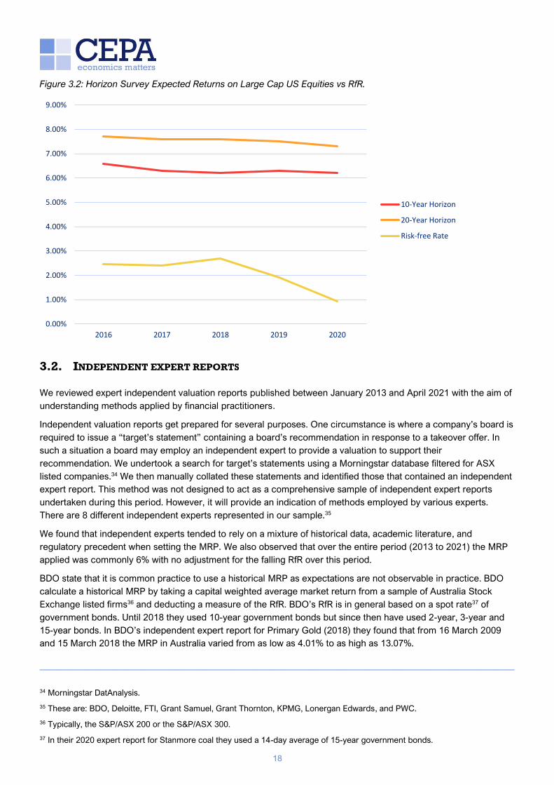
There are several other surveys which examine developments in other jurisdictions. One such example is Horizon
Actuarial Services LLC (Horizon), which conducts an annual survey of investment advisors in the USA. The survey
is targeted to investment advisors of multiemployer pension funds and similar investment firms. The survey asks
investment advisors to provide their “capital market assumptions” which include expected return of various assets
classes over 10-year and 20-year horizons. Horizon is consistent with their selection of surveyed investment
advisors and only reports historical data for investors who have responded to each of the annual surveys.
Therefore, we can be more confident that changes in responses year-to-year are the result of market conditions or
investors assumptions as opposed to changes in the mix of respondents.
The Horizon Survey suggests that although there has been a slight drop in investor expectations over recent years,
relative to changes in the RfR, expected equity returns in the USA have remained stable.
———————————————————————————————————————————————————
33 Includes 2013, 2015, 2017, 2018 and 2019.
18
Figure 3.2: Horizon Survey Expected Returns on Large Cap US Equities vs RfR.
3.2. INDEPENDENT EXPERT REPORTS
We reviewed expert independent valuation reports published between January 2013 and April 2021 with the aim of
understanding methods applied by financial practitioners.
Independent valuation reports get prepared for several purposes. One circumstance is where a company’s board is
required to issue a “target’s statement” containing a board’s recommendation in response to a takeover offer. In
such a situation a board may employ an independent expert to provide a valuation to support their
recommendation. We undertook a search for target’s statements using a Morningstar database filtered for ASX
listed companies.34 We then manually collated these statements and identified those that contained an independent
expert report. This method was not designed to act as a comprehensive sample of independent expert reports
undertaken during this period. However, it will provide an indication of methods employed by various experts.
There are 8 different independent experts represented in our sample.35
We found that independent experts tended to rely on a mixture of historical data, academic literature, and
regulatory precedent when setting the MRP. We also observed that over the entire period (2013 to 2021) the MRP
applied was commonly 6% with no adjustment for the falling RfR over this period.
BDO state that it is common practice to use a historical MRP as expectations are not observable in practice. BDO
calculate a historical MRP by taking a capital weighted average market return from a sample of Australia Stock
Exchange listed firms36 and deducting a measure of the RfR. BDO’s RfR is in general based on a spot rate37 of
government bonds. Until 2018 they used 10-year government bonds but since then have used 2-year, 3-year and
15-year bonds. In BDO’s independent expert report for Primary Gold (2018) they found that from 16 March 2009
and 15 March 2018 the MRP in Australia varied from as low as 4.01% to as high as 13.07%.
———————————————————————————————————————————————————
34 Morningstar DatAnalysis.
35 These are: BDO, Deloitte, FTI, Grant Samuel, Grant Thornton, KPMG, Lonergan Edwards, and PWC.
36 Typically, the S&P/ASX 200 or the S&P/ASX 300.
37 In their 2020 expert report for Stanmore coal they used a 14-day average of 15-year government bonds.
0.00%
1.00%
2.00%
3.00%
4.00%
5.00%
6.00%
7.00%
8.00%
9.00%
2016 2017 2018 2019 2020
10-Year Horizon
20-Year Horizon
Risk-free Rate
19
Grant Samuel use a blend of historical data and other analysts to formulate their MRP. In their independent expert
report for Acquila resources (2014), Grant Samuel cited the Officer study (2011) and stated their estimate of 6%
was similar to what other analysts use. In the same report Grant Samuel commented on the relationship between
MRP and the RfR:
“the market risk premium is not constant and changes over time. At various stages of the market cycle
investors perceive that equities are more risky than at other times and will increase or decrease their
expected premium. Indeed prior to 2008, there were arguments being put forward that the risk
premium was lower than it had been historically while today there is evidence to indicate that current
market risk premiums are above historical averages. However there is no accepted approach to deal
with changes in market risk premium for current conditions”.
Grant Samuel in their independent expert report for UGL (2016) made the following comment on the repricing of
risk after the global financial crisis:
“Anecdotal evidence suggests that equity investors have repriced risk since the global financial crisis
in 2007 and that acquirers are pricing offers on the basis of hurdle rates above those implied by
theoretical models. However this has yet to be translated into the measures of market risk premium (at
least those based on longer term historical data)”.
Similar to BDO, Grant Samuel take the spot rate of 10-year government bonds to calculate the RfR.
Grant Thornton base their MRP figure off empirical studies of up to 100 years. In their independent expert report for
Blackwood (2013) Grant Thornton said that their MRP was consistent with the MRP used by regulators such as the
Australian Competition and Consumer Commission (ACCC) and all other state regulators. Grant Thornton have
taken different approaches to calculating the RfR over the years, using a 10-day, 10-year, and “long-term” average
of 10-year government bonds in various reports.
In Lonergan Edwards independent expert report for CIMIC (2017) they cited a historical excess returns study by
Brailsford, Handley and Maheswaran (2008) as well as the Fernandez Surveys and evidence used by the AER. In
the same report Lonergan Edwards made the following comment on MRP during the global financial crisis.
“Prior to the GFC, independent experts in Australia generally adopted an MRP of around 6.0%. Whilst
the MRPs adopted by valuation practitioners (and regulatory bodies) generally increased for a
relatively short period following the GFC, they have subsequently returned to long-term historical
averages of around 6%”.
Lonergan Edwards consistently took a RfR of 4% in all their reports we reviewed. Their justification is that current
rates were artificially low compared to long-term averages due to quantitative easing both locally and
internationally. They would often compare 4% to spot rates on long term government bonds.
20
4. REGULATORY PRACTICE
We undertook case studies looking at the regulatory practice in three jurisdictions. These were the New Zealand
Commerce Commission (NZCC), Ofgem and the Federal Energy Regulatory Commission (FERC). The aim of the
case studies was to identify the evidence relied upon and reasoning applied by the regulator in making their MRP
assumption with specific focus on the relationship assumed between the RfR and MRP. Where we have identified
an instance where a regulator has explicitly examined the correlation between the RfR and MRP we have
highlighted it.
4.1. NEW ZEALAND COMMERCE COMMISSION
4.1.1. Current Approach
While the standard version of the CAPM assumes all sources of investment income are equally taxed at the
personal level, the New Zealand tax regime taxes capital gains and dividends less onerously than interest.
Therefore, the NZCC estimates a tax-adjusted market risk premium (TAMRP) instead of a standard MRP. This
assumes that:
• all dividends are fully imputed (i.e., shareholders receive an imputation credit based on tax paid by the
company which is used to reduce or eliminate their income tax liability);
• shareholders can fully utilise the credits;
• the average tax rate on dividends and interest is equal to the corporate tax rate; and
• capital gains are tax free.
Under these assumptions, the TAMRP is calculated as TAMRP = E(Rm) – Rf(1-Tc).38 When referring to the MRP in
the context of the NZCC’s approach we refer to the fact that their MRP has been adjusted for their unique tax
considerations.
The NZCC uses three approaches in estimating the MRP:
• studies of historical returns on shares relative to the RfR;
• surveys of investors asking them to state their expected rate of return for the overall market; and
• empirical estimates of the MRP from share prices and expected dividends.
The NZCC uses the following methods to estimate a value of the MRP:
• The Ibbotson approach (historical averaging of excess returns). The NZCC starts by averaging equity
returns in excess of the RfR for New Zealand from 1931 – 2018. A MRP is calculated using a three-year,
four-year, and five-year RfR.
• The Siegel 1 methodology, which adjusts the Ibbotson approach by replacing the historical RfR with an
estimated expected real RfR calculated from current yields on inflation-protected bonds.
• The Siegel 2 methodology, which assumes that total market returns are constant over time and therefore
converts the historic average real market return to a current nominal expected return using current inflation
forecasts and then deducts the current RfR.
———————————————————————————————————————————————————
38 Where, TAMRP = tax adjusted market risk premium, E(Rm) = expected market return, Rf = Risk-free rate and Tc = corporate
tax rate.

21
• Surveys of investors views on the MRP sourced from the Fernandez annual survey. The NZCC took a
median of responses. The reasons for taking a median over a mean are that the survey responses are
subjective views and that one can reasonably expect that some responses are frivolous or calculated in a
particular direction because respondents know that regulators use the survey.
• The DGM, which takes estimated future dividends and discounts them back to the existing market value of
the shares. The discount rate is the total market return from which the MRP can be calculated. Future
dividends are calculated taking estimates of futures dividends for the next 3 years, then the third-year
dividend growth rate is linearly converged over 8 years to the long-run growth rate (estimated by taking the
average of GDP growth from 1900 to 1938).
Summary of application of Siegel 1 methodology
Essentially the Siegel 1 methodology takes the Ibbotson type estimate for the MRP and then adds back the
estimated RfR used in the MRP calculation (arithmetic average of annual bond yields for the estimation period). An
expected RfR is then subtracted. Siegel (1992) recommends a RfR of 3-4%, the NZCC therefore uses a rate of
3.5%. More detail on the logic behind replacing the historic RfR with an expected long-term RfR is set out below.
For each year, the estimate of the Siegel 1 estimate of MRP is as follows:
MRP(Siegel) = MRP(Ibbotson) + Rf(1-Tc) – 0.035(1-Tc)
MRP(Siegel) = estimate of MRP using the Siegel 1 method
MRP(Ibbotson) = annual MRP from the Ibbotson method
Rf = RfR for that year used in the Ibbotson method
Tc = corporate tax rate
0.035 = midpoint between 3% and 4% used by Siegel as the long-term RfR.
Summary of application of Siegel 2 methodology
The Siegel 2 method assumes that the real market return is stable over time. Therefore, to estimate MRP, the
historic average market return is converted to a current nominal figure using a current inflation forecast and then
the current RfR is deducted.
The NZCC estimates the arithmetic average real market return using historical data from 1900-2018 (7.9%). This
figure is then converted to a current nominal expected market return using an expected inflation rate of 2%
(midpoint of RBNZ inflation target range). The result is 10.06%. Then the current RfR is deducted. Using the three-
year rate results in MRP of 9.5%.
MRP(Siegel 2) = [(1+LMr)*(1+i)-1]- Rf(1-Tc)
LMr = long term average return on the equity market %
i = current inflation forecast %
Summary of overall application
The NZCC then takes the median of the five different methods shown above, rounding to the nearest 0.5%. On this
issue of rounding the NZCC said:
“Dr Lally’s rationale for the rounding methodology was laid out by him in full in a report to the
Queensland Competition Authority which he refers to in his papers. He considers that the rounding
has little impact on the accuracy of the estimation measured through the standard error. However, its
value impact will incentivise submissions advocating an increase (or decrease) which adds to
administrative burden. Over time the small over and under estimations implicit (but essentially
unobservable) in a TAMRP rounded to the nearest 50bps will net out. In this respect it is not error in
any one regulatory period which matters, but error over the life of the assets.”
22
The NZCC considers that taking a broad approach not placing too much weight on a single methodology is more
likely to produce a better estimate. In its 2004 gas reviews decisions the NZCC said that each method has its
advantages and disadvantages, but all provide insight into the MRP. Lally favours using a median as it reduces the
impact on the estimate from an extreme outcome arising from one of the methods.39 The NZCC stated in their 2019
Fibre input methodologies (IMs):
“There is no consensus on a ‘correct’ methodology for estimating the TAMRP neither is there likely to
be a ‘correct’ weighting of the methodologies. We consider that there is no one best way to estimate
TAMRP and this is consistent with advice from Dr Lally. For our final decision we have considered all
information before us in reaching a judgement on the best estimate of TAMRP.”
As explained below the NZCC sees an advantage of using both Siegel 1 and Siegel 2 methods as they both have
different assumptions on the long-term stability of market return and MRP.
Where possible the NZCC calculates estimates for foreign countries to cross-check with their estimates for New
Zealand. The NZCC estimates these using the same method as they do for their New Zealand results, making slight
adjustments where necessary to account for tax differences. For their Ibbotson and Siegel estimations they take an
average of 19 different countries. For the dividend model they use only data from Australia. For survey data, the
NZCC takes a mean of the medians from 24 ‘developed countries’ in the Fernandez survey.
The NZCC also cross checks their results with estimates from investment banks and analysts. In 2019 the NZCC
used estimates of the MRP from 6 different investment banks.
The NZCC takes a median of responses in the surveys of investors views on the MRP.
4.1.2. Timeline of approaches
The NZCC publish input methodologies (IMs) which set out the rules, requirements and processes that must be
applied to regulation. The IMs are reviewed regularly and set out specific processes for calculating the various
parameters that make up the WACC. The contents of the IMs then flow through into decisions on setting the cost of
capital and other requirements regulated businesses face.
The NZCC has developed its approach for estimating MRP over the years although it has consistently used several
different methods.
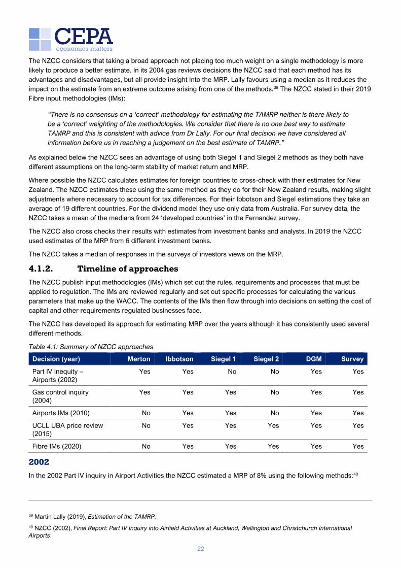
Table 4.1: Summary of NZCC approaches
Decision (year) Merton Ibbotson Siegel 1 Siegel 2 DGM Survey
Part IV Inequity –
Airports (2002)
Yes Yes No No Yes Yes
Gas control inquiry
(2004)
Yes Yes Yes No Yes Yes
Airports IMs (2010) No Yes Yes No Yes Yes
UCLL UBA price review
(2015)
No Yes Yes Yes Yes Yes
Fibre IMs (2020) No Yes Yes Yes Yes Yes
2002
In the 2002 Part IV inquiry in Airport Activities the NZCC estimated a MRP of 8% using the following methods:40
———————————————————————————————————————————————————
39 Martin Lally (2019), Estimation of the TAMRP.
40 NZCC (2002), Final Report: Part IV Inquiry into Airfield Activities at Auckland, Wellington and Christchurch International
Airports.

23
• Ibbotson approach;
• conversions of estimates of MRP into TAMRP;
• the Merton approach;
• Cornell dividend model; and
• surveys.
The Merton approach expresses MRP as proportional to market volatility (measured by variance or standard
deviation), estimates the coefficient of proportionality, and then applies this to a current estimate of market volatility.
The NZCC considered that this method was also subject to statistical uncertainty. The NZCC used an estimation
from Credit Suisse First Boston for the MRP using the Merton approach. This is discussed in more detail below.
The NZCC took estimates of the MRP from traditional CAPM models and adjusted these for New Zealand’s tax
situation. The NZCC considered that these estimates were a good check on estimates for the Ibbotson and Merton
approach.
The Cornell dividend model took estimates of dividend growth over the next 3 years and linearly converged these
estimates to long run GDP growth (taken from an estimate from NZIER) over 20 years.
The estimations ranged from 7.5% to 9.4% (although this figure was considered biased up by 1%), the NZCC
therefore estimated the MRP to be 8% with a lower bound of 7% and an upper bound of 9% given the statistical
uncertainty surrounding the historical methods.
2004
In the 2004 gas control inquiry the NZCC estimated a MRP of 7%. The NZCC used five different methods: Ibbotson,
Siegel 1, Merton, Cornell and surveys. This time the NZCC took a median of the five different methods. The NZCC
took the view in this decision that all methods have their advantages and disadvantages, but all provide insights into
the MRP. Therefore, it prefers to consider a wide range of estimation approaches. Their reasons for introducing the
Siegel method are expanded on below.
2010
In the 2010 Airports IMs, the NZCC did not include the Merton approach in its estimations. The reason for this was
that although the Merton approach has a sound theoretical basis, it was not considered as empirically robust, as the
estimation results have significant standard errors. Therefore, the approach for the 2010 IMs was to take the
median of the Ibbotson approach, the Siegel 1 approach, DGM, and Surveys. The reasons for abandoning the
Merton method are expanded on below.
2015
In the 2015 UCLL and UBA pricing reviews the Siegel 2 method was introduced. The method was introduced as an
alternative approach to address the pronounced unanticipated inflation the Siegel 1 method addresses. Advice
received by Martin Lally considered that there is value in this method beyond addressing historic inflation shocks.41
The method assumes that expected real market return is stable over time and this may be a better assumption than
under the Siegel 1 method, which assumes that MRP is stable over time. The NZCC accordingly considers both
methods. The approach used in the 2015 UCLL and UBA pricing reviews is the same as the current method.
4.1.3. Summary of reasoning for including or removing each method
Ibbotson
In the 2002 part IV airports inquiry, the NZCC said this on the use of historical averaging to estimate MRP:
———————————————————————————————————————————————————
41 Martin Lally, “Review of submissions on the risk-free rate and TAMRP for UCLL and UBA services”, 2015.

24
“There are a number of ways of estimating this parameter. The most widely used is to observe the ex-
post annual counterparts to each term comprising the market risk premium, and then arithmetically
average over a large number of years. The methodology was first applied by Ibbotson and Sinquefield
(1976) to the market risk premium in the standard version of the Capital Asset Pricing Model”.
The NZCC took the arithmetic mean of the historical averages citing a paper by Cooper (1996)42 for their reasoning:
“The use of arithmetic mean ignores estimation error and serial correlation in returns. Unbiased
discount factors have been derived that correct for both these effects. In all cases, the corrected
discount rates are closer to the arithmetic mean than the geometric mean.”
The NZCC mentioned that there are issues around selecting the period to use when estimating the MRP:43
“The choice of timespan involves a trade-off between more data (which improves the statistical
precision of the estimate, assuming the true value has not changed over time) and potentially less data
(in so far as the true value has changed over time). I favour the longer timespan, and hence the 0.082
estimate.”
The NZCC states that there are several more fundamental issues with the method.44
“The most significant may be the statistical uncertainty surrounding the estimate. Chay et. al (1993,
Table 5) give a standard deviation for the annual figures used in estimating the New Zealand market
risk premium for the standard CAPM of .22, for the years 1931-92”.
“Other concerns with the methodology include the use of listed equity as a proxy for the market
portfolio (Roll, 1977; Roll and Ross, 1994; Lally 1995). Potential biases arising from unexpected
inflation post WWII period (Siegel, 1999), and changes over time in the true value, arising from
changes in factors such as market volatility. The last two factors suggest that the results from historical
averaging overestimate the current value of the market risk premium”.
Siegel
The NZCC introduced the Siegel 1 method in its 2004 gas control inquiry. On Siegel 1, Lally advised:
“He shows that the Ibbotson type estimate of the standard MRP is unusually high using data from
1926-1990, due to very low returns on bonds in that period. He further argues the latter is attributable
to pronounced unanticipated inflation in that period. Consequently, the Ibbotson type estimate of the
standard MRP is biased up when using data from 1926-1990.”45
The unanticipated inflation is said to have caused significantly lower real returns on bonds. The reason being that
investors of bonds in 1960s and 1970s did not know there was going to be large inflation in the future, therefore this
future inflation was not priced into the bonds and the real return on bonds during this period was significantly low.
Therefore, this caused an unusually higher MRP than other periods looked at by Siegel. From Siegel (1992)46 on the
impact on MRP:
———————————————————————————————————————————————————
42 Cooper, Ian. (1996), Arithmetic versus Geometric Mean Estimators: Setting Discount Rates for Capital Budgeting”, European
Financial Management, vol.2. pp.157-67
43 NZCC (2002), p. 476.
44 NZCC (2002), p. 477.
45 Martin Lally (2005), The weighted average cost of electricity lines businesses.
46 Siegel, J. (1992), The Equity Premium: Stock and Bond Returns Since 1802. Financial Analysts Journal, 48, 28-38.

25
“The decline in the real return on fixed income investments has meant that the advantage of holding
equities, which have experienced a remarkably steady real return, has increased over time. The equity
premium, plotted in Figure I, has trended up over the last 200 years and was particularly high in the
middle of this century. The premium, computed from real geometric returns, averaged 0.6 per cent in
the first subperiod, 3.5 per cent in the second, and 5.9 per cent in the third. The primary source of this
equity premium has been the fall in the real return on bonds, not the rise in the return on equity.
Nonetheless, it is not unreasonable to believe that the low real rates on bonds may, on occasion, have
fueled higher equity returns, because the costs of obtaining leverage were so low. The highest 30-year
average equity return occurred in 1931-61, a period that also experienced very low real returns on
bonds.”
The NZCC introduced the Siegel 2 method in the 2015 UCLL and UBA pricing reviews. The method was introduced
as an alternative to the unanticipated inflation shock described by Siegel. On Siegel 2, Lally advised:
“An alternative approach to the inflation-shock issue raised by Siegel (1992, 1999) arises from Siegel’s
observation that the average real market return was similar across the three subperiods examined by
him, leading him to conclude that the expected real market return was stable over time. Accordingly,
one would estimate the expected real market return from the historical average, convert to its nominal
counterpart today using a current inflation forecast, and then deduct the current RfR (net of tax)” 47
The NZCC considers that both approaches are useful as they both have different assumptions on the long-term
stability of TMR and MRP.
“Furthermore, since both versions seek to address the late 20th century inflation shock, they might be
considered to be alternatives rather than complementary. However, the second version has merit
independent of any historical inflation shock because it assumes that the expected real market return
is stable over time and this may be a better assumption than that underlying the historical averaging of
excess returns (that the TAMRP is stable over time).” 48
“The Siegel 1 methodology implicitly assumes no relationship between the MRP and RfRs, while the
Siegel 2 methodology implicitly assumes that there is an inverse correlation between the two
parameters. Therefore, across the methodologies that we apply, we allow for different assumptions on
the relationship between the MRP and RfRs.” 49
DGM
The NZCC received advice from Lally acknowledging the difficulty in estimating parameters for DGM but that it held
an advantage is that it does not face the same wide confidence intervals of historical based approaches:
“Like the earlier approaches, this forward-looking approach has a number of drawbacks. These
include uncertainty about expected dividend growth rates and the period of convergence towards the
long-run rate, the assumption that the observed market price of the market portfolio is rationally set,
and that the model used by the market in setting km corresponds to that invoked here in equation (1).
Bearing these concerns in mind, the above results of its application favours an estimate of the market
risk premium of less than .08. LECG (2001) appear to dismiss approaches of this kind due to the
considerable uncertainties involved in assessing various parameters. However they are free of the
wide confidence intervals that characterize historical averaging.”
———————————————————————————————————————————————————
47 Lally (2015), Review of submissions on the risk-free rate and TAMRP for UCLL and UBA services.
48 Ibid.
49 New Zealand Commerce Commission (2020), Fibre Input Methodologies Reasons Paper.

26
Merton
The Merton approach assumes the MRP changes overtime. A paper by Merton (1980)50 suggests that MRP is
proportional to either market variance or standard deviation of returns and key to this is the assumption that MRP
varies over time. The logic being that holding interest rates (and other market factors) constant, if the risk in the
market increases then return demanded by the market will increase and therefore the MRP will increase:
“At the extreme where market is riskless, then by arbitrage [Total market returns = RfR], and the risk
premium on the market will be zero. If the market is not riskless, then the market must have a positive
risk premium. While not always the case, a generally reasonable assumption is that to induce risk-
averse investors to bear more risk, the expected return must be higher. Given that, in aggregate, the
market must be held, this implies that, ceteris paribus, the equilibrium expected return on the market is
an increasing function of the risk of the market.”
“Of course, if changes in preferences or in the distribution of wealth are such that aggregate risk
aversion declines between one period and another, then higher market risk in the one period need net
imply a correspondingly higher risk premium. However, if aggregate risk aversion changes slowly
through time by comparison with the changes in market risk, then, at least locally in time, one would
expect higher levels of risk to induce a higher market risk premium.”
If it can be assumed that MRP is some function of risk in the market, estimating this relationship and applying to a
current estimate of market risk would yield an estimate of the MRP. Merton (1980) expresses MRP as proportional
to market volatility (variance or standard deviation), estimates the coefficient of this proportionality and then applies
it to current market risk. In the 2002 airport part IV decision the NZCC used results from a 1998 Credit Suisse First
Boston report51, which (according to the NZCC the methodology from the paper had not been fully disclosed)
differed slightly from Merton and had yet to appear in financial or economic literature.
Boyle (2005)52 applies the Merton methodology to the New Zealand market. Boyle expresses the MRP as a function
of the variance of market returns and observes that variance is much easier to estimate than the mean of returns,
particularly when these parameters vary over time.53 Boyle estimates a “market price of risk” in place of MRP,
where the market price of risk is equal to variance on returns multiplied by the average risk aversion of the market.
The Merton method was ultimately scrapped in the 2010 airport IMs. The NZCC noted:
“Whilst Merton has a sound theoretical foundation, it has also been viewed as one of the least robust
methods empirically because of the significant standard errors associated with the estimated results.
Consequently, the Commission places no weight on the resulting Merton ex post estimates in its
decisions following Dr Lally’s recommendation.”
Martin Lally further expanded on the Merton method in his advice given on setting the WACC for electricity
networks in 2005:
“More recently, Boyle (2005) has used this Merton methodology to estimate the market risk premium
in the standard CAPM, for each year in the period 1970-2003. Volatility is defined as variance and is
simply estimated from the preceding three years of data. The resulting estimates for the market risk
———————————————————————————————————————————————————
50 Merton, Robert C. (1980), On Estimating the expected return on the market: an exploratory investigation. Journal of financial
economics (v8), pp323-61.
51 We are unable to locate this report.
52 Glenn Boyle, (2005), Risk, expected return, and the cost of equity capital. New Zealand Economic Papers, Taylor & Francis
Journals, vol. 39(2), pages 181-194.
53 Boyle argues that a fairly accurate estimate of variance can be obtained so long as the data is high frequency, whilst to
estimate an accurate mean you need a long time series of data.

27
premium vary from .009 to .336, due to variation in the estimates for variance… Such implausible
variation in the market risk premium leads Boyle to conclude that this methodology cannot be relied
upon. The source of the problem is the unreliable estimates of variance, and the use of only three
years of data to do so contributes to that problem. Clearly the use of a very long period for estimating
volatility would be inconsistent with the presumption of intertemporal variation in volatility that
underlies this methodology. So there is a trade-off here in choosing the period for estimating volatility,
and no clear basis for determining the optimal period.”54
4.2. OFGEM, UK
4.2.1. Introduction
This review of the development of Ofgem’s regulatory approach considers the evolution of how Ofgem has treated
the relationship between the RfR and MRP. This means the focus is on how the cost of equity parameter is
established in each price control. In many cases, the relationship between the RfR and MRP was not explored
explicitly at each price review, but the decisions made provide an implicit model for the relationship.
We focused on tracking the development of the regulatory approach on distribution price controls and the evidence
and reasoning considered. MRP and RfR are parameters common across the sectors Ofgem regulates. As such,
the development of the regulatory approach is relatively consistent across the sectors. We started our review at the
Distribution Price Control Review 4 (DPCR4) which ran from April 2005 to March 2010.
4.2.2. DPCR4
The starting point for the development of DPCR4 was the Developing network monopoly price controls paper in
June 2003.55 We consider this to be a key period in the development of the regulatory approach which currently
prevails in the UK. It is in this paper that Ofgem first refers to the 2003 Wright, Mason and Miles (WMM) paper
which makes a strong recommendation for the aggregate equity return approach which is now referred to by the
AER as the ‘Wright’ approach.56 We consider that Ofgem places substantial weight on the findings of WMM and this
influences the development of DPCR4 and subsequent price controls.
WWM “regard the standard approach to building up the cost of equity, from estimates of the safe rate and the
equity premium, as problematic. [They] would recommend, instead, that estimates should be derived from
estimates of the aggregate return (the cost of equity for the average firm), and the safe rate.” In our opinion the
paper advances three separate but connected arguments for applying this approach:
1. A re-expression of the CAPM pricing equation as a weighted average of the RfR and the expected market
return.
2. A theoretical argument based on the RfR puzzle and equity premium puzzle.
3. An empirical argument based on the relative stability of the total market return.
The starting point for WWM’s argument is a simple re-expression of the CAPM equation:
𝐸(𝑅𝑖) = 𝑅𝑓 + 𝛽𝑖(𝐸(𝑅𝑚) − 𝑅𝑓)
𝐸(𝑅𝑖) = (1 − 𝛽𝑖)𝑅𝑓 + 𝛽𝑖(𝐸(𝑅𝑚))
The second equation shows that the expected return on a firm’s equity can be re-expressed equivalently as the
weighted average of the RfR (with weight 1 – β) and the expected market return (with weight β). This means that the
closer a given firm’s β is to 1 the lower the implied weight of the safe rate. WWM conclude that “regulated
———————————————————————————————————————————————————
54 Martin Lally (2005), The Weighted Average Cost of Capital for Electricity Lines Businesses.
55 Ofgem (2003), Developing network monopoly price controls, June.
56 Smithers & Co (2003), A study into certain aspects of the cost of capital for regulated utilities in the UK, February.

28
industries are unlikely to be “precisely” average, with a beta of unity, but none the less the dominant element in
their cost of capital will always be the expected stock market return”.
The second part of the argument is based on economic theory. WWM point out that standard CAPM is not
“designed to explain the common components: these are simply used as inputs to such models.” They argue that
to find an explanation it is necessary to examine the “fundamental determinants of asset prices”. To do this WWM
turn to consumption CAPM (CCAPM) models. CCAPM models are one set of economic models and it is sufficient
for our purposes here to simply outline some key features of a simple CCAPM model:57
• A CCAPM is a multi-period model with a single representative investor who maximises utility over time by
choosing between various alternative assets. The consumption of this representative investor could be
represented by the average consumption level in the economy.
• The investor is assumed to have diminishing marginal utility of consumption. When the level of consumption
is already high, the benefit they receive from the next unit of consumption is lower than if the same increase
in consumption were to occur at a lower level of consumption. The investor is also considered risk-averse;
they want smooth consumption over all periods.
• As in CAPM, in CCAPM the relationship between rates of return depends on the correlation of these
returns with some benchmark. In CCAPM this is the marginal utility of consumption.
• Investors prefer to consume money today rather than in later periods. This means that to induce investment
the rate of return needs to be set such that investors become indifferent between consumption today and
consumption in later periods.
• If there is a correlation between consumption and the rate of return of the investment, then this depresses
the expected benefit. This is because the rate of return will be high when consumption is already high. This
is effectively an anti-insurance product. To get the investor to purchase anti-insurance they need a higher
rate of return.
WWM conclude that these models provide a good rationale for why stocks should yield higher returns than safe
assets. Safe assets have zero correlation with consumption while good news for the economy as a whole is
correlate with good news for consumption and high returns on shares.
WWM quote Mehra and Prescott (1985) who establish that there is an equity premium puzzle. Mehra and Prescott
find that while the data was consistent with the qualitative features of CCAPM theory (i.e. RfR is lower than MRP)
they could not account for the magnitude of the gap. The observed covariance between stock returns and
aggregate consumption is low meaning that the magnitude of the difference can only be explained by assuming
that marginal utility varies a lot in response to small changes in consumption. This means that risk-aversion must be
very high.
In addition to the equity premium puzzle, WWM add the “risk-free rate puzzle”. In this case WWM quote Weil (1989)
who concluded that the high level of risk-aversion can only be reconciled with the low historic average risk-free
rates observed in the data if the representative investor is assumed to prefer consumption tomorrow over
consumption today. This reverse order of preference is “massively counter-intuitive”.
WWM conclude that both these puzzles are “two sides of the same coin”. In contrast to the failure of this theory to
explain the relative historic returns on equities versus safe investments (i.e., the ERP) it is possible to derive
expected stock returns that are consistent with historical averages with modest levels of risk-aversion and time-
preference. WWM then demonstrate exactly this finding but conclude that the implied RfR is higher and equity risk
———————————————————————————————————————————————————
57 A seminal paper is Lucas (1978), Asset prices in an Exchange Economy. We understand that there are more advanced
CCAPM models than the one described here and referenced by WWM in their argument.

29
premium is lower than historic data suggests.58 They conclude that there is a “clear inconsistency between theory
and data rela[ted] to the safe rate, and hence the equity premium.”
The final part of WWM’s argument relates to the empirical data. In contrast to “uncertainty about the true historic
risk-free rate, and hence the equity premium” they find “a range of evidence the equity return has, over reasonably
long samples, been fairly stable both over time, and across different markets.”
After considering the evidence, both drawing on theory and empirical evidence, WWM loop back to the first
argument that the CAPM equation can be re-stated. The dominant element being the expected market return is
seen as “fortunate for the regulators, since [they] argue that there is considerably more uncertainty about the true
historic risk-free, and hence equity premium, then there is about the market return itself.”
Ofgem summarises the WWM conclusion by stating that “if the value of beta is equal to one, there is no need to
calculate the equity risk premium and the risk free rate of return separately and it may be preferable to focus on the
aggregate market equity return.” Ofgem goes on further to conclude that “given the uncertainty surrounding
estimates of the inputs into CAPM, Ofgem sees merit in considering the aggregate return on equity alongside the
traditional building block approach. The relative weight…will depend on…the extent to which the equity risks of the
regulated business are similar to the market average.”
In March 2004, as part of the DPCR4 process, Ofgem published a further paper.59 This paper provides Ofgem’s
initial estimates of the cost of capital for this price control. Ofgem provides two approaches to calculating the cost of
equity:
• The main method where the RfR and ERP are estimated separately. The ERP is estimated using Dimson,
Marsh and Staunton (DMS) data.60 DMS calculates an annualised ERP relative to bond returns.
• An alternative method, the aggregate return on equity approach, which they attribute to WWM. This is
summarised as a method to be used “in situations where there is considerable uncertainty with respect to
the risk free rate and ERP, an aggregate equity return approach might be more appropriate. This would not
require judgements with respect to the cost of equity…but it would require an assumption that equity beta
is approximately 1.”
The Ofgem final proposals paper places further emphasis on the aggregate return on equity approach.61 The
reason for this was a further paper by Smithers & Co which looked at beta estimates for electricity and water
companies. They found “strong evidence of parameter instability” with one possible interpretation being “beta
estimates are more uncertain and hence more weight might be given to a beta assumption of 1”. The finding that
more weight should be placed on assuming beta is 1 neatly ties with the overall aggregate return on equity
approach.
4.2.3. DPCR5
DCPR5 was a price control which ran from 1 April 2010 to 31 March 2015. The start of this process is Ofgem’s
initial consultation document in March 2008.62 The paper outlines that there are two approaches where “cost of
equity can either be assessed by determining the risk-free rate, an equity risk premium for the market and an
equity beta…or by an aggregate return on equity” [emphasis added]. There is an observation that long-term
average rates of return had been between 6.5 to 7.5 percent but that it was too soon to determine whether this was
an appropriate range for the cost of equity.
———————————————————————————————————————————————————
58 See Figure 2.1 in Smithers & Co (2003).
59 Ofgem (2004), Electricity Distribution Price Control Review – Background information on the cost of capital, March.
60 Dimson, Marsh, Staunton (2001), Millennium Book II – 101 Years of Investment Returns.
61 Ofgem (2004), Electricity Distribution Price Control Review – Final Proposals, November.
62 Ofgem (2008), Electricity Distribution Price Control Review – Initial consultation document, March.

30
The three elements of the cost of equity (RfR, ERP and beta) are referenced as separate elements. 63 The key piece
of evidence examined for ERP is the DMS dataset. Our understanding is that Ofgem considered DMS’s historic
excess returns evidence as part of their decision on ERP.64 In addition, Ofgem points to Bank of England
commentary stating that the “risk premium for UK equities, which had been extremely elevated in March, had
returned to around its average of the past decade”. Finally, Ofgem also presents evidence that “utilities, especially
regulated companies, are less risky than the market and therefore have an equity beta of less than one.”
4.2.4. RIIO-ED1
The RIIO-ED1 price control started on 1 April 2015 and will run to 31 March 2023. As with DPCR5, the consultation
makes clear that there are two alternative approaches to the cost of equity: “the cost of equity can either be
assessed by determining the risk-free rate, an equity risk for the market and an equity beta…or an aggregate return
on equity.”
During the consultation Ofgem set out a CAPM-based cost of equity with estimates for each parameter. The RfR
was estimated based off the historical (5/10 year) average inflation-linked gilt yields.
Ofgem state that their “preferred approach [for the ERP] is to rely on well-established long term ERP estimates
provided by Dimson, Marsh and Staunton”. They state that DMS “assessed excess return on equities relative to
sovereign bonds in 19 developed countries over more than 100 years (since 1990)”. Ofgem also highlights
evidence submitted which demonstrates that the DMS methodology provides a lower estimate during a downturn.
They point to a “number of academics” that have argued that the ERP rises at the time of financial crisis, as
investors seek a higher return to compensate for the perceived increase in risk. Ofgem concludes that this would
place their preferred estimate around the upper end of DMS’s range.
Ofgem re-engaged with the issue of assessing equity market returns a few months later following a Competition
Commission (CC) provisional determination for Northern Ireland Electricity (NIE).65 NIE was not regulated by Ofgem
but the CC’s successor body (the Competition and Markets Authority, CMA) would become the appeal body for
RIIO-ED1 determinations. The key issue in the appeal was whether to place greater weight on “contemporary
market evidence.”66
Ofgem commissioned Wright and Smithers (W&S) to re-consider the issues.67 W&S observe that until the CC
provisional determination UK regulators had employed the methods outlined in the 2003 report fairly consistently.
Namely that the “real market cost of capital should be assumed constant, on the basis of data from long-term
historic averages of realised stock returns.” W&S conclude there is some evidence that long-term estimates based
on their method have fallen but this can be attributed to updated data and changes to inflation assumptions.
W&S advise against any model “in which the expected market return is assumed to have been pulled down by falls
in the risk-free rate”. W&S seem to re-state the evidence that was covered in the 2003 report, namely that there is
no evidence of stability of the RfR and by extension no evidence of the stability of MRP. They conclude that there is
“no empirical basis for the assumption that falls in risk-free rates should translate to falls in expected market
returns.” They further advise that they “do not rule out using the contemporary market evidence on the risk-free
rate…[but] simply argue that the current risk-free rate should not play a role in estimating the market cost of
equity”. Finally, on addressing the observed valuation premium of regulated companies they suggest that this is
due to a beta being set close to one “despite strong evidence that it is much closer to around one half” (0.5).
———————————————————————————————————————————————————
63 Ofgem (2009), Electricity Distribution Price Control Review Final Proposals – Allowed Revenues and Financial Issues,
December.
64 NERA (2009), Distribution Network Operators’ Cost of Capital for DPCR5.
65 Ofgem (2013), Consultation on our methodology for assessing the equity market return for the purpose of setting RIIO price
controls, December.
66 Ofgem provides a long list of a wide range of “contemporary” evidence considered by the CC, see page 4 of Ofgem (2013).
67 Wright and Smithers (2013), The Cost of Equity Capital for Regulated Companies: A review for Ofgem.

31
In Ofgem’s decision on methodology, which is maintained in their RIIO-ED1 final determination, they decided to give
“greater weight to the influence of current market conditions in relation to the equity market return”.68 Ofgem
observe that even under a Smithers & Co model a “low risk-free rate will reduce the cost of equity for relatively low
systematic risk businesses, even if equity market returns were assumed constant”. Furthermore, there is evidence
that observed market betas are lower than 0.9 or 0.95 assumed previously.
4.2.5. RIIO-2
While RIIO-ED1 will continue to run until 31 March 2023, final determinations have been made by Ofgem for RIIO-2
for Transmission and Gas Distribution network companies and the Electricity System Operator. We can use these
final determinations to see how Ofgem’s approach has evolved since 2015.
In their RIIO-2 framework consultation Ofgem makes reference to an updated report for the UK Regulators Network
(UKRN).69 This report made ten recommendations for regulatory practice including “Recommendation
5…Regulators should continue to base their estimate of the TMR on long-run averages, taking into account both UK
and international evidence.”70
The sector specific methodology consultation sets out the broad approach that Ofgem adopted for RIIO-2, which at
a high-level is maintained until final determination.71 We observe no attempt to estimate ERP as an independent
parameter. The cost of equity is set using the equation below with total market returns (TMR) estimated with a
contemporary estimate of the RfR:
𝐶𝑜𝐸 = 𝑅𝐹𝑅 + 𝛽(𝑇𝑀𝑅 − 𝑅𝐹𝑅)
The 2018 Wright et al paper shows some evolution in thinking since 2003 on several issues related to cost of capital
estimation.72 However, recommendation 5 re-affirms the use of long-run historic averages of total market returns for
setting the ERP parameter. While the recommendation has not changed, we consider the relative focus of the
evidence has shifted. The argument they put forward for their approach can be summarised as follows:
• Wright et al observe “apparent stability of long-run returns on mature stock markets, especially in
comparison with the considerably lesser degree of stability of returns on other major asset classes.”
Evidence is presented showing the similarity in long-run average returns in UK, US, and world markets
excluding the US.
• There has been a substantial fall in the real RfR, but this is not historically unprecedented. Ex-post real
interest rates were distinctly more negative in the 60s and 70s than in recent years. The implication of this
is “ex-post the equity premium has been very far from stable.”
• Wright et al consider three alternatives to the total market return approach and whether developments in
academic evidence and financial practice have “undermined the MMW methodology”:
o The first alternative considered is assume the ERP is stable. They consider that the “empirical basis
for this assumption was always weak” and that this approach is undermined as the “evidence for
counter-cyclical risk premia is strong”.
———————————————————————————————————————————————————
68 Ofgem (2014), Decision on our methodology for assessing the equity market return for the purpose of setting RIIO-ED1 price
controls.
69 Ofgem (2018), RIIO-2 Framework Consultation.
70 Wright et al (2018), Estimating the cost of capital for implementation of price controls by UK Regulators – An update on
Mason, Miles and Wright (2003).
71 Ofgem (2018), RIIO-2 Sector Specific Methodology Annex: Finance.
72 We understand that Wright has contributed an additional paper as part of the CMA appeals process in the UK. However, this
paper was not publicly available at the time this report was written.
32
o The second alternative is to update the estimate of TMR in line with econometric evidence of return
predictability.73 They conclude that evidence of return predictability (e.g., Shiller) undermines the
MMW methodology. However, despite evidence of this predictability, MMW conclude there are no
obvious “implementable” or “defensible” mechanism for regulators to update TMR using this
evidence.
o The third alternative is to estimate TMR using an alternative model such as a DDM. Again, while
MMW conclude there is merit to these approaches they could not find an implementable or
defensible methodology for using a DDM to calculate the TMR.
4.3. FERC, USA
4.3.1. FERC’s mandate
In the US, the Federal Energy Regulatory Commission (FERC) regulates interstate electricity transmission, as well
as gas and oil pipelines and wholesale power. FERC derives much of its authority from Sections 205 and 206 of the
Federal Power ACT.74 Section 205 provides that:
“[a]l rates and charges … for or in connection with the transmission or sale of electric energy … and
all rules and regulations affecting or pertaining to such rates and charges shall be just and
reasonable.”75
Section 206 empowers FERC to: 1) initiate a proceeding to determine whether any transmission charges or rates
are not just and reasonable; and 2) determine the just and reasonable charge/ rate to be observed thereafter.76
An important consideration in FERC’s decisions are the capital attraction standards set in “Hope” and “Bluefield”,
two Supreme Court cases that require FERC “to set a rate of return commensurate with other enterprises of
comparable risk and sufficient to assure that enough capital is attracted to the utility to enable it to meet the public's
needs.”77
4.3.2. Until 2014
FERC has traditionally relied on a “one-step” Discounted Cash Flow model (DCF) in setting the return on equity
(RoE) of public electric utilities under its jurisdiction.
The DCF model is similar to the DGM/DDM models used by Australian and overseas regulators. However, rather
than using it to derive an estimate of total market returns, FERC used the DCF to directly estimate the RoE for an
individual utility. Specifically, FERC used the DCF to derive cost of equity estimates for each company in a ‘proxy
group’ of electric utilities, then set the regulated utility’s RoE at a level within the ‘zone of reasonableness’ (i.e., the
range of estimates for the proxy group), typically the midpoint or the median.78
This method estimates RoE directly, without separately identifying RfR and MRP or providing a view of the
relationship between these parameters and total market returns.
———————————————————————————————————————————————————
73 For consistency with the preceding sections, we refer to total market returns (TMR) here while Wright et al uses the shorthand
EMR.
74 Congressional Research Service (2020), The Legal Framework of the Federal Power Act, January, p. 2.
75 United States Code (USC), Title 16, s. 824d.
76 United States Code (USC), Title 16, s. 824e.
77 FERC (2020), para. 4.
78 FERC (2014), para. 26.

33
4.3.3. After 2014
Additional evidence considered
In Opinion 531 (2014), setting the RoE for the New England transmission owners (NETOs), FERC departed from its
typical midpoint approach.
FERC explained that evidence of anomalous capital market conditions, including bond yields that were at historic
lows, made it less confident that the midpoint of the DCF-based zone of reasonableness accurately reflected the
RoE necessary to meet the Hope and Bluefield capital attraction standards. 79 FERC therefore looked to alternative
sources of evidence in addition to the DCF method, including the Risk Premium model and CAPM, to derive
allowed RoE.80
Based on these alternative methods, all of which indicated higher RoE compared to the DCF, FERC decided to set
RoE at the midpoint of the upper half (i.e., the upper quartile) of the zone of reasonableness produced by the DCF
model. A similar uplift to the midpoint of the DCF zone of reasonableness was applied by FERC in a number of
subsequent RoE decisions.81
It is also worth noting that in Opinion 531, for the purposes of the DCF method, FERC started relying on a “two-
step” procedure for determining the dividend growth component of the model.82 This consists in averaging short-
term and long-term growth estimates, based on five-year analyst forecasts for each company in the proxy group83
and GDP growth, respectively.84
FERC had previously relied on a “one-step” DCF, with dividend growth assumptions based only on short-term
analyst forecasts, as it considered the US electricity sector was in a phase of restructuring and it would have been
too speculative to assume that investors were reflecting long-term growth estimates in their investment decisions.85
However, by 2014 FERC considered it was appropriate to update this aspect of the methodology, as a two-step
approach would be more in line with the underlying theory of the DCF.86
Elimination of the ‘Treasury Bond Update’
One instance in which FERC explicitly considered the relationship between RfR and RoE (and thus, indirectly,
between the RfR and MRP) is the decision to abandon the ‘Treasury Bond Update’.
Until 2014, the FERC established RoE based on evidence available at the time of the case. However, recognising
that capital market conditions can change between the date the utility files its case and the date FERC issues a final
decision, FERC updated the RoE at the time of the final decision. FERC’s long-standing practice was to base this
post-hearing adjustment on the change in U.S. Treasury bond yields during the same time period. The premise
underlying the use of U.S. Treasury bonds for the post-hearing RoE adjustment was that changes in RoE over time
track changes in U.S. Treasury bond yields.87
However, in Opinion 531, FERC considered that U.S. Treasury bond yields did not provide a reliable and consistent
metric for tracking changes in RoE. The Commission noted:
———————————————————————————————————————————————————
79FERC (2014), paras. 144-145.
80 FERC (2020), Opinion n. 569-A, para. 4.
81FERC (2020), paras 6 and 8.
82 FERC (2014), para 36.
83 As published by the Institutional Brokers Estimate System (IBES).
84 FERC (2014), para. 17.
85 FERC (2014), para. 24-25, 29-31.
86 FERC (2014), para 36.
87 FERC (2014), Opinion 531(Docket No. EL11-66-001), 19 June 2014, para. 157.

34
“while U.S. Treasury bond yields are an important indicator of capital market conditions and therefore
inform our determination of an appropriate base RoE, the capital market conditions since the 2008
market collapse and the record in this proceeding have shown that there is not a direct
correlation between changes in U.S. Treasury bond yields and changes in RoE. Therefore, the
premise underlying the Commission’s use of U.S. Treasury bond yields for post-hearing RoE
adjustments is not always accurate.”88 [emphasis added]
FERC cited the following evidence in support of this opinion:
• In Southern California Edison Company, a 2008 case in which the post-hearing adjustment was at issue,
expert testimony indicated that, as U.S. Treasury bond yields decreased, DCF results instead went up,
suggesting an inverse relationship between U.S. Treasury bond yields and utility RoE.
• The record in the proceedings leading to Opinion 531 also showed an inverse relationship over the course
of six months between 2012 and 2013. The record in this proceeding also cast doubt on the magnitude of
the relationship between U.S. Treasury bond yields and utility RoE (FERC’s practice traditionally had been
to adjust the RoE using a 1:1 correspondence between the RoE and the change in U.S. Treasury bond
yields) and suggested that for every basis point the U.S. Treasury bond yields change, FERC should adjust
the RoE by a fraction of that amount.
Therefore, FERC abandoned the ‘Treasury Bond Update’ approach. Instead, FERC concluded that a more
reasonable approach was to allow the participants in a rate case to present the most recent financial data available
at the time of the hearing as up-to-date evidence of the appropriate RoE.89
4.3.4. 2020 RoE decision
In Order 569-A (2020), establishing the RoE for the Midcontinent Independent System Operator (MISO)
transmission owners, FERC landed on using three methods, with equal weight,90 to establish RoE for public utilities:
DCF, CAPM, and the Risk Premium model. Specifically, FERC established a zone of reasonableness for each
method, then averaged the top and bottom of the three zones to identify a composite zone of reasonableness. In
Order 569-A, FERC set RoE at the midpoint of the composite zone.91
DCF
In 2020, the Commission reaffirmed its use of a two-step DCF analysis, giving 20% weight to a long-term growth
rate based on GDP growth, and 80% weight to a short-term growth rate based on analyst forecasts.92
CAPM
FERC describes the CAPM method as follows:
“the CAPM methodology estimates the cost of equity by taking the “risk-free rate” and adding to it the
“market-risk premium” multiplied by “beta.” […] The market risk premium is calculated by subtracting
the risk-free rate from the expected return. The expected return can be estimated either using a
backward-looking approach, a forward-looking approach, or a survey of academics and investment
professionals.”93
———————————————————————————————————————————————————
88FERC (2014), para 158.
89FERC (2014), para. 160.
90 FERC (2020), para 141.
91 FERC (2020), para 214.
92 FERC (2020), para. 57.
93 FERC (2019), Opinion n. 569, para 229.

35
In recent rate decisions, FERC relied on a forward-looking approach, using a DCF to estimate expected returns.
Specifically, FERC derived a CAPM ‘zone of reasonableness’ for RoE by:
• Estimating the expected return for each dividend paying members of the S&P 50094 by applying a one-step
DCF model, 95 with a dividend growth assumption based on IBES three to five year consensus growth
projections.96
• using the 30-year U.S. Treasury bond average historical yield over a six-month period as the risk-free
rate;97 and
• taking the difference between the two to obtain an estimate of MRP98 that can be plugged in the CAPM
formula to derive a RoE estimate for each company, thus deriving a range of RoE estimates which
determine the zone of reasonableness.99
This method effectively implies a negative correlation between RfR and MRP for a given level of total market returns
estimated through the DCF. It is also worth noting that in the past FERC rejected CAPM analyses that were based
on historical excess returns.100
Risk Premium model
The Risk Premium model estimates cost of equity using the implied premium provided by regulatory decisions and
settlements over Baa-rated utility bonds. FERC explains the logic of this method as follows:
“The risk premium methodology, in which interest rates are a direct input, is “based on the simple idea
that since investors in stocks take greater risk than investors in bonds, the former expect to earn a
return on a stock investment that reflects a ‘premium’ over and above the return they expect to earn
on a bond investment.” As the NETOs explain, investors’ required risk premiums expand with low
interest rates and shrink at higher interest rates. The link between interest rates and risk premiums
provides a helpful indicator of how investors’ required returns on equity have been impacted by the
interest rate environment.”101 [emphasis added]
This suggests the Risk Premium model is also based on a view that RfR and MRP are to some extent inversely
related.
———————————————————————————————————————————————————
94 FERC (2019), Opinion n. 569, para 260. Note, some S&P500 companies are excluded from the analysis, for example when
FERC consider they have abnormal returns.
95 FERC found that the rationale for incorporating a long-term growth rate estimate in the DCF analysis of a specific group of
utilities does not apply when conducting a DCF study of the companies in the S&P 500 index under the CAPM method. FERC
noted that: 1) as the index is regularly updated to represent the overall market, with companies with declining stock values and
market capitalisation replaced by companies with growing stock values, it is not unrealistic to assume its short term growth to
extend into the future; and 2) the index includes large, mature companies with limited growth potential – this already reflects a
consideration that companies cannot maintain indefinitely the high growth rates of their early years, without requiring a transition
to GDP-growth for the longer-term. FERC (2019), paras. 263-266.
96 FERC (2019), para. 274.
97 FERC (2019), Opinion n. 569, para 238.
98 FERC (2019), para 239.
99 FERC (2019), para. 437.
100 FERC (2014), para. 147, footnote 292.
101FERC (2014), para 147.

36
5. OBSERVATIONS ON DATA
5.1. OUR APPROACH
The AER asked us to investigate whether the MRP moves through time, and whether there is any relationship with
the RfR. The MRP is a forward-looking concept: it is the expected return on the market less the RfR. The direct
estimates of the MRP using the averages of the historic realised MRP cannot therefore be used to assess whether
the MRP changes through time, as they do not measure what the forward looking MRP was at the time.
To explore whether MRP shifts over time we made estimates using forward looking approaches. We considered two
approaches: DGMs and earnings yield models.
Our analysis of the data is exploratory in nature and is at most a preliminary assessment of the empirical evidence.
Dividend Growth Models
DGMs assume that the value of a security, or the overall stock market, is the discounted value of its future
dividends, and this is equal to the dividend yield plus expected growth in dividends. With observations on the yield,
and assumptions on growth in dividends, the cost of equity can be derived as the DGM’s discount rate. There are a
range of detailed assumptions that are typically required to implement DGMs: the number of stages; the sources of
estimates of growth and whether there are biases in these estimates; how injections and withdrawals of equity are
taken account of; and the relationship between long-term dividend growth and economic growth. These
assumptions should be based on forward-looking forecasts but are often based on historic information.
The range of plausible assumptions mean that implementations of the DGM can produce a wide range of estimates
of the cost of equity for the market (a flaw that also applies to other CAPM based approaches to the cost of
equity).102 However, while there may be uncertainty about the level of the cost of equity that is derived using a
DGM, a consistent approach to estimating the DGM using historic series may allow one to derive a historic time
series of estimates of the contemporaneous cost of equity. We also observe that others have found that ERPs
estimated using a variety of DGMs are fairly strongly correlated and their results move together through time.103
In this paper, we have derived time series of the cost of equity for Australia using the DGM in a simple approach.
We do not assert that the levels of these estimates should be used in a determination of the cost of equity by the
AER. However, we consider that the changes in the cost of equity in the series provide a good indication of the
changes in the forward-looking returns expected by investors at the time.
We use a two-stage DGM, with a first stage based on estimates of dividend growth and a second stage where
growth is equal to long-term GDP growth minus a 1% adjustment to account for net creation of shares from new
companies and new share issues from existing companies.104 Using this specification, we derive two cost of equity
series by:
• Estimating the DGM in each year between 1917 and 2016 using outturn data.105 This relies on a
historical dividend yield series based on RBA and Datastream data. Long-term growth is a 40-year average
of future GDP growth rates, based on a historical Australian GDP series compiled by the Department of
———————————————————————————————————————————————————
102 We observe that Partington and Satchell (2016) highlight many of the criticisms of DGMs. These include slow changes to
estimated cost of equity because of sluggish adjustments to changing expectations of growth, potential upward biases in inputs
(for example using analyst dividend forecasts), issues with the appropriate sample of firms being used and the fact that results
can vary substantially depending on the specification applied. Partington and Satchell (2016), Report to the AER, Cost of Equity
Issues.
103 Duarte and Rosa (2015), The Equity Risk Premium: A Review of Models.
104 The 1% deduction is in line with Lally, M. (2013), Review of the AER’s proposed Dividend Growth Model, December, p. 5-6.
105 Series time periods dependent on data availability.
37
Foreign Affairs and Trade (DFAT)106 up to 2017 and an assumption that, after 2017, nominal GDP grows
annually by 5.6%.107 This analysis assumes that market participants form expectations on dividends and
growth that are in line with future outcomes.
• Estimating the DGM in each year between 2005 and 2020 using forecast data on dividend yields (from
Bloomberg) and GDP growth (from the International Monetary Fund (IMF)). Unlike the DGM based on
outturn data, this analysis does not require a strong assumption on market participants’ expectations. This,
however, limits the analysis to the shorter period over which dividend forecast data is available.
Our approach and the associated data sources are set out in detail in Appendix A. We consider that the results of
our DGM analyses (as any DGMs, as discussed above) are likely to be influenced by input data, assumptions, and
model specification. In particular, the input data on outturn dividend yields and GDP growth we used in our analysis
required data transformations and combining multiple data sources. In addition, the results from our DGM based on
outturn data appear to be particularly sensitive to the length of the averaging period used to set long-term growth
assumptions. We discuss this further in Section 5.2.
Earnings yield models
The earnings yield is the ratio between the earnings of a stock, or the overall stock market, and the stock price.
Earnings yield models are less commonly observed than DGMs but are derived in similar ways. If firms are in stable
growth and there are no excess profits, it can be shown (e.g., Damodaran 2021)108 that the earnings yield is the cost
of equity. However, if the assumption of no excess earnings is relaxed or if one assumes growth in earnings can be
maintained with a full dividend pay-out,109 the earnings yield would be somewhat lower than the cost of equity.
There is also an issue as to whether the yield measures the cost of equity in real or nominal terms: if a forward
measure of earnings is used this is likely to include an inflation expectation, and so in practice the measure is likely
to reflect nominal expectations.
As with the DGM approach, there are substantial difficulties in calibration of earnings yield models. But as with
DGMs, changes in the estimate of cost of equity using earnings yield models are likely to be indicative of changes in
the cost of equity (see Damodaran 2021). Shiller is well known for his analysis of stock market valuations using the
CAPE (Cyclically Adjusted Price Earnings) ratio.110 He has recently adjusted his use of the CAPE ratio, estimating a
“CAPE yield”. For a range of markets, he has constructed time series estimates of the CAPE yield, and estimated
models where the expected return on equity is assumed to equal a constant plus the CAPE yield (Shiller 2020).
This has been shown to provide a good fit of the subsequent returns on equity markets. The conclusion is that
measures of earnings yield can be used as part of an approach to estimate the forward-looking cost of equity.111
We estimate two cost of equity series using earnings yield models:
———————————————————————————————————————————————————
106 DFAT, "australias-trade-and-economic-indicators-historical.xlsx", https://www.dfat.gov.au/trade/resources/trade-
statistics/Pages/trade-time-series-data, accessed May 2021.
107 This assumption is also in line with Lally (2013).
108 Damodaran (2021), Equity Risk Premiums (ERP): Determinants, Estimation, and Implications – The 2021 Edition, March, p. 82.
109 This is the view, for example, in Richards, A.J. (1991), The cost of equity capital in Australia: What can we learn from
international equity returns?, RBA Research Discussion Paper 9107, September, p. 5-6.
110 Shiller (2000), Irrational Exuberance.
111 We observe that Partington and Satchell (2017) have argued against using the earnings yield as an indicator of changes in
the cost of equity, on the basis that the earnings yield is a consequence of interactions between the cost of equity, the growth
rate, and the dividend pay-out ratio. See Partington and Satchell (2017), Report to the AER: discussion of estimates of the return
on equity, April, p. 21-22. However, the argument that the earnings yield may fail to pick up variations in the cost of equity due to
contemporaneous changes in the growth rate appears to be at odds with Damodaran’s (2021) characterisation of the earnings
yield and more broadly with the assumption of stable growth used in DGMs, from which the earnings yield can be derived .
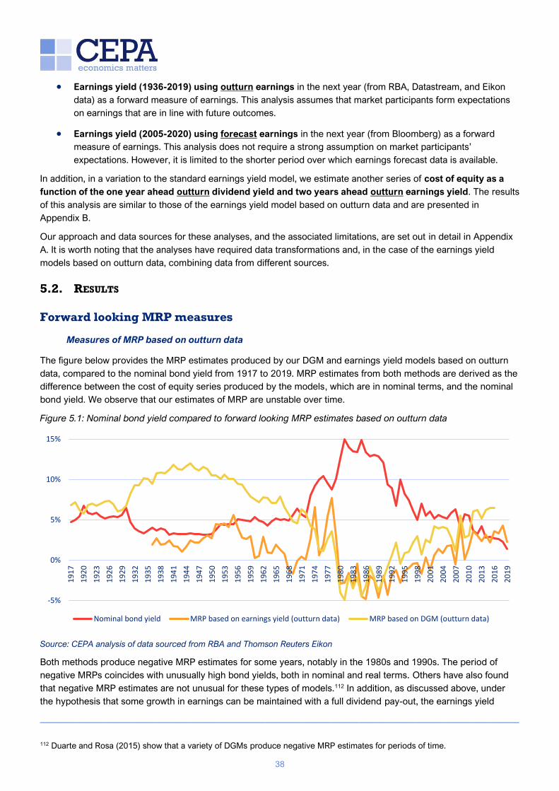
38
• Earnings yield (1936-2019) using outturn earnings in the next year (from RBA, Datastream, and Eikon
data) as a forward measure of earnings. This analysis assumes that market participants form expectations
on earnings that are in line with future outcomes.
• Earnings yield (2005-2020) using forecast earnings in the next year (from Bloomberg) as a forward
measure of earnings. This analysis does not require a strong assumption on market participants’
expectations. However, it is limited to the shorter period over which earnings forecast data is available.
In addition, in a variation to the standard earnings yield model, we estimate another series of cost of equity as a
function of the one year ahead outturn dividend yield and two years ahead outturn earnings yield. The results
of this analysis are similar to those of the earnings yield model based on outturn data and are presented in
Appendix B.
Our approach and data sources for these analyses, and the associated limitations, are set out in detail in Appendix
A. It is worth noting that the analyses have required data transformations and, in the case of the earnings yield
models based on outturn data, combining data from different sources.
5.2. RESULTS
Forward looking MRP measures
Measures of MRP based on outturn data
The figure below provides the MRP estimates produced by our DGM and earnings yield models based on outturn
data, compared to the nominal bond yield from 1917 to 2019. MRP estimates from both methods are derived as the
difference between the cost of equity series produced by the models, which are in nominal terms, and the nominal
bond yield. We observe that our estimates of MRP are unstable over time.
Figure 5.1: Nominal bond yield compared to forward looking MRP estimates based on outturn data
Source: CEPA analysis of data sourced from RBA and Thomson Reuters Eikon
Both methods produce negative MRP estimates for some years, notably in the 1980s and 1990s. The period of
negative MRPs coincides with unusually high bond yields, both in nominal and real terms. Others have also found
that negative MRP estimates are not unusual for these types of models.112 In addition, as discussed above, under
the hypothesis that some growth in earnings can be maintained with a full dividend pay-out, the earnings yield
———————————————————————————————————————————————————
112 Duarte and Rosa (2015) show that a variety of DGMs produce negative MRP estimates for periods of time.
-5%
0%
5%
10%
15%
19
17
19
20
19
23
19
26
19
29
19
32
19
35
19
38
19
41
19
44
19
47
19
50
19
53
19
56
19
59
19
62
19
65
19
68
19
71
19
74
19
77
19
80
19
83
19
86
19
89
19
92
19
95
19
98
20
01
20
04
20
07
20
10
20
13
20
16
20
19
Nominal bond yield MRP based on earnings yield (outturn data) MRP based on DGM (outturn data)

39
would be somewhat lower than the cost of equity – which might help explain the relatively low level of the MRP
based on the earnings yield model.
As part of these analyses, we are not claiming that the DGM and earnings yield model produce accurate measures
of the MRP, but merely that they can be used to provide a consistent estimate of the directional changes in MRP.
We would consider it suggestive of a potential relationship if several such specifications of forward-looking
measures of the MRP provided the same directional relationship when compared with the RfR.
We use the nominal bond yield as a proxy for the RfR. In the absence of a long historical data series of the “ex ante”
real RfR (i.e., the nominal bond yield minus expected inflation), we can compare MRP with either the nominal RfR or
the “ex post” real RfR (i.e., the nominal bond yield minus outturn inflation). The ex post real RfR is affected by
inflation shocks, i.e., unexpected swings in inflation that would not be factored in a forward-looking MRP estimate.
Therefore, we consider that a comparison with the nominal RfR is more appropriate.
To investigate the relationship between MRP and RfR, we fit a simple Ordinary Least Squares (OLS) regression
model:
𝑀𝑅𝑃𝑡 = 𝛼 + 𝛽𝑅𝐹𝑅𝑡 + 𝜀𝑡
We estimated the model over the whole length of the series as well as in the period from 1993 onwards, based on a
hypothesis that there is a change in the relationship at the advent of central bank inflation targeting. Even if no such
structural break is assumed, we observe that the strength of the relationship seems to change between the earlier
and latter periods of the data.
For the DGM-based estimate, over both time periods, we observe a strong negative relationship between MRP and
RfR. R-squared, a standard measure of model goodness of fit, is high in both cases. The negative coefficients in this
analysis, and all those presented in the remainder of this section, are statistically significant at the 1% level. This
finding is confirmed when computing standard errors that are robust to autocorrelation. Detailed statistical
information, including standard errors, levels of statistical significance, confidence intervals, and number of
observations are presented in Appendix B.
Figure 5.2: MRP (vertical axis) vs nominal bond yield (horizontal axis). MRP measured as DGM cost of equity
estimate (based on outturn data) minus nominal bond yield. DGM assumes long-term growth equal to 40-year
average of GDP growth.
Source: CEPA analysis of data sourced from RBA and Thomson Reuters Eikon
The results of the DGM appear to be sensitive to underlying assumptions. In particular, the relationship over the
whole series becomes weaker, with a considerably lower R-squared, when considering a DGM focused on shorter
term growth expectations, where the averaging period for the growth assumption is of five rather than 40 years (see
Figure 5.3 below). After 1993, the relationship also becomes weaker, but the model retains a relatively good fit.
In this case, a shorter averaging period results in a more volatile long-term growth assumption, leading to sharper
fluctuations in the cost of equity and MRP, which in turn obscures to some extent the relationship with the RfR.
y = -1.26x + 0.13R² = 0.79
-8%
-6%
-4%
-2%
0%
2%
4%
6%
8%
10%
12%
14%
2% 4% 6% 8% 10% 12% 14% 16%
1917-2016
y = -1.10x + 0.09R² = 0.91
-8%
-6%
-4%
-2%
0%
2%
4%
6%
8%
10%
12%
14%
2% 4% 6% 8% 10% 12% 14% 16%
1993-2016

40
While it could be argued that a short averaging period is too strongly driven by phases of the business cycle and (to
some extent unexpected) economic shocks to provide a long-term growth assumption, this result illustrates the
sensitivity of the DGM results to specific assumptions.
Figure 5.3: MRP vs nominal bond yield. MRP measured as DGM cost of equity estimate (based on outturn data)
minus nominal bond yield. DGM assumes long-term growth equal to 5-year average of GDP growth.
Source: CEPA analysis of data sourced from RBA and Thomson Reuters Eikon
For the earnings yield-based estimate of the MRP, over the whole series, we observe a relatively weak negative
relationship with the RfR, with a slope of -0.47 and a relatively low R-squared of 0.38. The negative relationship
becomes stronger and clearer in the period after 1993.
Figure 5.4: MRP vs nominal bond yield. MRP measured as earnings yield (based on outturn data) minus nominal
bond yield.
Source: CEPA analysis of data sourced from RBA and Thomson Reuters Eikon
Measures of MRP based on forecast data
As set out above, in addition to long time series based on outturn data, we have constructed estimates of the cost
of equity based on dividends and earnings forecasts sourced from Bloomberg. While these series are shorter, as
forecasts are only available from 2005 onwards, they allow us to relax the assumption of rational expectations
implicit in the analysis of outturn data.
The figure below provides the MRP estimates produced by our DGM and earnings yield models based on forecast
data, compared to the nominal bond yield from 2005 to 2020. MRP estimates from both methods are derived as the
difference between the cost of equity series produced by the models, which are in nominal terms, and the nominal
bond yield. Again, the estimates of MRP appear to be unstable over time.
y = -0.86x + 0.11R² = 0.28
-10%
-5%
0%
5%
10%
15%
20%
2% 4% 6% 8% 10% 12% 14% 16%
y = -0.47x + 0.04R² = 0.38
-6%
-4%
-2%
0%
2%
4%
6%
8%
10%
0% 2% 4% 6% 8% 10% 12% 14% 16%
1936-2019
1917-2016
y = -0.93x + 0.09R² = 0.61
-10%
-5%
0%
5%
10%
15%
20%
2% 4% 6% 8% 10% 12% 14% 16%
1993-2016
y = -0.88x + 0.06R² = 0.75
-6%
-4%
-2%
0%
2%
4%
6%
8%
10%
0% 2% 4% 6% 8% 10% 12% 14% 16%
1993-2019

41
Figure 5.5: Nominal bond yield compared to forward looking MRP estimates based on forecast data
Source: CEPA analysis of data sourced from Bloomberg
The figures below present the results of regression models of these MRP measures against the nominal RfR. In both
cases, we observe a strong negative relationship, although the R-squared is higher in the DGM analysis.
Figure 5.6: MRP vs nominal bond yield. MRP measured as DGM cost of equity estimate (based on forecast data)
minus nominal bond yield.
Source: CEPA analysis of data sourced from Bloomberg
0%
2%
4%
6%
8%
10%
2005 2006 2007 2008 2009 2010 2011 2012 2013 2014 2015 2016 2017 2018 2019 2020
MRP based on earnings yield (forecast data) MRP based on DGM (forecast data)
Nominal bond yield
y = -0.90x + 0.09R² = 0.78
0%
2%
4%
6%
8%
10%
0% 2% 4% 6% 8% 10%
2005-2020

42
y = -0.61x + 0.10R² = 0.25
0%
2%
4%
6%
8%
10%
12%
14%
16%
-5% 0% 5% 10% 15%
Figure 5.7: MRP vs nominal bond yield. MRP measured as earnings yield (based on forecast data) minus nominal
bond yield.
Source: CEPA analysis of data sourced from Bloomberg
Ex post assessment
While the appropriate measure of the cost of equity is an ex-ante one, we have also examined the relationship
between the measured returns on equity over 10-year periods and compared these to the 10-year return on an
investment in a risk-free instrument over the same time period. This is then a comparison of the returns that an
investor would get by investing in two different instruments. This is different from the Ibbotson or Dimson, Marsh,
Staunton type analysis which measures the average of returns on long term bonds held over a year; we measure
the long term bonds as if held to maturity.
The chart below shows these 10-year ex post returns over two time periods: 1892-2020, and 1993-2020. As with
our ex-ante return measures, there is a weak inverse relationship between the MRP and RfR over the longer period,
whereas since 1993, the relationship appears to be stronger.
Figure 5.8: Ex-post MRP vs RfR in 10-year rolling periods, 1892-2020 and 1993-2020
Source: CEPA analysis of data sourced from AER
y = -0.75x + 0.06R² = 0.53
0%
2%
4%
6%
8%
10%
0% 2% 4% 6% 8% 10%
y = -0.28x + 0.07R² = 0.09
0%
2%
4%
6%
8%
10%
12%
14%
16%
-5% 0% 5% 10% 15%
1892-2020 1993-2020
2005-2020

43
5.3. OTHER MARKETS
The motivation for our analysis of forward-looking estimates of the risk-free rate came from an analysis of US
markets. Damodaran publishes his estimate of the implied equity risk premium on an annual basis.113 The figure
below shows this estimate plotted against risk-free rates, both for his entire series of 1961-2020 and separately
from 1993-2020.
Over the full series there is no clear relationship with risk-free rates, but, similarly to Australia, over the last 25 to 30
years there is a strong negative relationship between expected equity returns and risk-free rates.
Figure 5.9: Damodaran’s implied ERP premium (FCFE) vs RfR
Source: CEPA analysis of Damodaran (2020)
5.4. OBSERVATIONS
We note that the analyses presented in this section are exploratory in nature and likely to be sensitive to input data
and assumptions. However, the models we estimated on Australian data suggest a negative relationship between
the MRP and the RfR across different measures of cost of equity, albeit with varying magnitude and goodness of fit.
The relationship appears to be stronger in more recent years, from the 1990s and possibly earlier. We have not
undertaken econometric testing to detect a statistically significant structural break, but it does appear that the
relationship is weaker in the earlier part of the dataset. It is possible that the action of central banks from the 1990s
to set monetary policy settings to drive out inflation had a material impact on asset returns and investor
expectations. Prior to this period, monetary policy was less disciplined, and less predictable. The move to a more
stable relationship between these variables from the 1990s is consistent with this hypothesis.
———————————————————————————————————————————————————
113 Damodaran provides the following description for his implied equity risk premium measure – “Risk premiums are estimated
based upon a simple 2-stage Augmented Dividend discount model and reflect the risk premium which would justify they [sic]
current level of the index, given the dividend yield, expected growth in earnings and the level of the long term bond rate.”
y = -0.01x + 0.04R² = 0.00
0%
1%
2%
3%
4%
5%
6%
7%
0% 5% 10% 15%
1961-2020 1993-2020
y = -0.67x + 0.07R² = 0.75
0%
1%
2%
3%
4%
5%
6%
7%
0% 2% 4% 6% 8% 10%
1993-2020

44
6. RECOMMENDATIONS AND FURTHER WORK
The AER interprets its duties under the NEO and NGO as that “we consider that an efficient return for risk should
be estimated through a forward-looking rate of return using relevant market data.”114
The analysis above addresses many fundamental issues about the MRP. In our discussion here, we comment
narrowly on the issues that we have been asked by the AER to address, i.e. whether there is relationship between
the MRP and the risk free rate. We do not consider the evidence on the weight to be placed on forward looking
return estimates.
Our assessment is that (i) there is acceptance that MRP is not stable and (ii) it is possible that there is an inverse
relationship between the forward looking MRP and the risk-free rate, (iii) there is no good evidence that the MRP
should be assumed to be independent of the RfR the current assumption of the AER, and (iv) there is no conclusive
theoretical basis for an assumption of independence or dependence.
Further empirical work could lead to a more robust assessment of the evidence. That could include alternative
formulations of MRP, and econometric analysis. Following such additional work, we suggest that the AER considers
three options for estimation of the MRP from historical data:
• Fixed MRP approach: Estimation of the MRP is based on the assumption that it is stable and can be
estimated from the premium observed in historical data. In Australia this is often referred to as the Ibbotson
approach. Under this approach a perfect positive correlation between the RfR and TMR is assumed.
• Fixed TMR approach: Estimation of the MRP is based on the assumption that the total market return (TMR)
is stable and can be estimated from historical data. In Australia this is often referred to as the Wright
approach. Under this approach a perfect negative correlation between the RfR and the MRP is assumed.
• Hybrid approach: This approach would place weight on both of the above approaches. It relies on an
assumption that there is a negative correlation between the RfR and the MRP but this correlation is not
perfect, so that a fall (/rise) in the risk free rate would lead to a rise (/fall) in the MRP, but the change in the
MRP would be smaller than that of the risk free rate. Analysis of historical data or alternative approaches
could be used to calibrate the model.
Our review of international regulators demonstrates that regulatory processes can accommodate any of these
approaches. The data to implement these for Australia is available. Each of them is subject to error, and potentially
reliability can be made acceptable by combining estimates. The fact that each approach has been adopted in some
respect by other regulators indicates that they are sufficiently simple to be accepted by stakeholders.
The evidence indicates that the second two alternatives cannot be ruled out, and may provide better estimates of
the forward looking MRP consistent with the AER’s duty. We suggest that consideration of these options, and the
evidence that would be necessary to decide between them is undertaken as part of the 2022 RORI process.
———————————————————————————————————————————————————
114 AER (2018), Draft Rate of return Guidelines – Explanatory Statement.

45
COST OF EQUITY MODEL SPECIFICATIONS AND DATA SOURCES
The table below presents the equations and assumptions underlying our analyses of the correlation between RfR and MRP using earnings yield and the DGM. It also
indicates data sources, data transformations required to carry out the analysis, and limitations.
Approach Earnings yield
(outturn)
Earnings yield
(forecast)
Earnings yield 2 years ahead
(outturn)
DGM
(outturn)
DGM
(forecast)
Measure of
Cost of Equity
Forward earnings yield based on
outturn earnings data.
Forward earnings yield based
on earnings forecasts.
Cost of equity as a function of
one year ahead dividend yield
and two years ahead earnings
yield. Based on outturn earnings
and dividend data.
The equations underlying this
approach are set out in
subsection A.1.
The DGM assumes that the share price is equal to the
discounted value of future dividend payments, using CoE
as the discount rate. We implement two versions of a two-
stage DGM, with a similar specification. One uses outturn
dividends (Div) and outturn GDP growth (g) as “ex post”
measures of expected dividend growth in the shorter term
(i.e., the first N years ahead plus the remaining fraction m
of the current year) and longer term, respectively. The
other model is based on forecast dividends and GDP
growth at time t.
Equation115
Data sources
(years
covered)
Note: all
Australian
stock
exchange data
are for the
ASX100, for
consistency
with RBA’s
Price:
• RBA: market cap (1936-72)
• Eikon: mkt value (1973-2019)
Earnings:
• RBA: P/E ratio (1937-73)
• Datastream (reported by RBA): P/E
ratio (1974-2018)
• Eikon: P/E ratio (2019-20)
• Bloomberg: current year and
year ahead expected P/E
ratios (2005-2020)
Price:
• RBA: mkt cap (1935-72)
• Eikon: mkt value (1973-2017)
• RBA: price index (1935-78)
• Datastream (reported by RBA):
price index (1979-2018)
Earnings:
• RBA: P/E ratio (1937-74)
• Datastream (reported by RBA):
P/E ratio (1975-2018)
Price:
• RBA: price index (1917-78)
• Datastream (reported by RBA):
price index (1979-2018)
Dividends:
• RBA: dividend yield (1936-73)
• Datastream (reported by RBA):
dividend yield (1974-2018)
GDP:
Dividend yield:
• Bloomberg: current year,
year ahead, and 2-years
ahead expected dividend
yields (2005-21)
GDP growth:
• Based on IMF’s World
Economic Outlook
(2005-21) 6-years ahead
forecasts of real GDP
growth and inflation.
———————————————————————————————————————————————————
115 The subscript t denotes a variable as at 31 December of year t. For earnings and dividends the subscript t denotes the quantity accrued between 31/12/t-1 and 31/12/t.
𝐶𝑜𝐸𝑡 =𝐸𝑎𝑟𝑛𝑖𝑛𝑔𝑠𝑡+1
𝑃𝑟𝑖𝑐𝑒𝑡 𝐶𝑜𝐸𝑡 =
𝐸(𝐸𝑎𝑟𝑛𝑖𝑛𝑔𝑠𝑡+1)
𝑃𝑟𝑖𝑐𝑒𝑡 𝐶𝑜𝐸𝑡 = 𝑓
𝐷𝑖𝑣𝑡+1
𝑃𝑡;𝐸𝑎𝑟𝑛𝑖𝑛𝑔𝑠𝑡+2
𝑃𝑡

46
Approach Earnings yield
(outturn)
Earnings yield
(forecast)
Earnings yield 2 years ahead
(outturn)
DGM
(outturn)
DGM
(forecast)
historical
dataset
Dividends:
• RBA: dividend yield (1936-73)
• Datastream (reported by RBA):
dividend yield (1974-2018)
• DFAT: nominal GDP (1901-
2017)
• After 2017, GDP is assumed to
grow by 5.6% p.a. (as per
assumption in AER’s 2013 and
2018 RORI)
Model
specification/
data
transformations
required
All sources report the trailing P/E
ratio (i.e., price divided by earnings in
previous 12 months), whereas we are
interested in comparing prices with
forward-looking 12-month earnings.
As the P/E ratio is the index market
cap divided by company earnings, we
can calculate earnings as market cap
divided by P/E. We then calculate the
forward earnings yield as earnings in
t+1 divided by market cap in t.
We want to consider forward
earnings yield as of 31/12 (for
consistency with AER’s
inflation and bond yield data).
However, Bloomberg only
provides expected earnings
by financial year (ending
30/06).
To resolve this mismatch, we
average Bloomberg’s
expected P/E ratio for the
current FY with the expected
P/E ratio for the next FY.
We then calculate the inverse
of this average P/E ratio to
obtain the earnings yield.
All sources report the trailing
dividend yield (i.e., dividends in
previous 12 months divided by
current price). We convert
dividend yield from trailing to
forward looking by dividing it by
the current price index and
multiplying it by the index 12
months prior.
We calculate the 2 years ahead
earnings yield as earnings in t+2
divided by market cap in t.
• Years of expected dividend
growth before model
converges to long-term
growth: N=2
• Long-term growth rate: g =
average nominal GDP
growth rate between t+N
and t+N+40 ( we also run a
sensitivity with an averaging
period of five years), minus
a 1% adjustment for the net
creation of new shares from
new companies and new
share issues (net of
buybacks) from existing
companies.
• The model is estimated as
at 31/12/t and assumes the
year ends on 31/12/t,
therefore dividends for the
remainder of the current
year are 0.
• A similar transformation as
described in the other
methods is required to
convert trailing dividend
yields into forward-looking
yields.
• N=2
• g = nominal GDP
growth rate (IMF 6yr
forecast) -1%.
• The model is
estimated as at 31/12/t
and assumes the year
ends on 30/06/t+1,
therefore the dividend
yield for the remainder
of the current year is
half the total dividend
yield expected for the
current year.

47
Approach Earnings yield
(outturn)
Earnings yield
(forecast)
Earnings yield 2 years ahead
(outturn)
DGM
(outturn)
DGM
(forecast)
MRP
calculation
MRP = earnings yield – nominal bond
yield
MRP = earnings yield –
nominal bond yield
MRP = earnings yield – nominal
bond yield
We calculate MRP as the nominal cost of equity (estimated
through the DGM, which uses nominal growth) minus the
nominal bond yield.
Notes and
data limitations
RBA notes that its market cap series
includes all companies for which
there is data, but the ratios (e.g. P/E)
include only companies for which
there is information for both the
numerator and the denominator,
which may result in small
discrepancies between ratios and
aggregates.116
Note: the transformation
described above may
introduce discrepancies if
earnings are not uniformly
distributed throughout each
FY.
RBA notes that its market cap
series includes all companies for
which there is data, but the ratios
(e.g. P/E, dividend yield) include
only companies for which there is
information for both the
numerator and the denominator.
What we tested is merely one of many possible
specifications of the DGM. DGM results are likely to be
sensitive to a range of assumption, including on: the
number of stages; the sources of estimates of growth and
whether there are biases in these estimates; how injections
and withdrawals of equity are taken account of; and the
relationship between long term dividend growth and
economic growth.
Other sources of data used in all models:
• Nominal bond yield – AER Historical Excess Returns model, where the bond yield is calculated as the one-year return on the 10-year Commonwealth Government
bond.
• Inflation – AER Historical Excess Returns model.
———————————————————————————————————————————————————
116 See Info in “Sydney Stock Exchange Historical Data.xlsx” published alongside Mathews, T. (RBA, 2019), A history of Australian equities, Research Discussion Paper 2019-04.

48
EARNINGS YIELD TWO YEARS AHEAD
The equations below describe how we derived our estimate of cost of equity based on the two years ahead
earnings yield.
Assuming:
𝐶𝑜𝐸 =𝐸𝑡+2
𝑃𝑡+1
and:
𝑃𝑡+1 = (1 + 𝐶𝑜𝐸)𝑃𝑡 − 𝐷𝑡+1
We obtain:
𝐶𝑜𝐸 =𝐸𝑡+2
(1 + 𝐶𝑜𝐸)𝑃𝑡 − 𝐷𝑡+1
𝐶𝑜𝐸(1 + 𝐶𝑜𝐸)𝑃𝑡 − 𝐷𝑡+1𝐶𝑜𝐸 = 𝐸𝑡+2
𝐶𝑜𝐸(1 + 𝐶𝑜𝐸) −𝐷𝑡+1
𝑃𝑡𝐶𝑜𝐸 =
𝐸𝑡+2
𝑃𝑡
𝐶𝑜𝐸2 + 1 −𝐷𝑡+1
𝑃𝑡 𝐶𝑜𝐸 −
𝐸𝑡+2
𝑃𝑡= 0
Let:
𝑏 = 1 −𝐷𝑡+1
𝑃𝑡
and:
𝑐 = −𝐸𝑡+2
𝑃𝑡
Then the cost of equity is equal to the positive solution of:
𝐶𝑜𝐸 =−𝑏 ± √𝑏2 − 4𝑐
2

49
REGRESSION RESULTS AND STATISTICAL TESTS
This section provides detailed results from the regression analyses presented in this report. For each model, a table
provides regression coefficients (with heteroskedasticity robust standard errors in parentheses below) and their
level of statistical significance (“***” indicates statistical significance at the 1% level). We provide 95% confidence
intervals based on the reported standard errors, as well as 95% confidence intervals based on Newey –West
standard errors robust to heteroskedasticity and autocorrelation up to a specified lag.117
REGRESSION RESULTS – OUTTURN DATA
Whole sample
Table A 1: MRP vs nominal bond yield. MRP based on DGM (outturn data) with long-term growth equal to 40-year
average of GDP growth.
Table A 2: MRP vs nominal bond yield. MRP based on DGM (outturn data) with long-term growth equal to 5-year
average of GDP growth.
———————————————————————————————————————————————————
117 We tested Newey-West regressions with the order of autocorrelation suggested by the results of the stata command “actest”.
Where actest did not indicate that autocorrelation of any order was statistically significant at a 5% level, we do not report
autocorrelation robust confidence intervals. Note, Newey-West regressions produce the same coefficients as the baseline OLS
regressions. All Newey-West regression coefficients are also statistically significant at the 1% level.
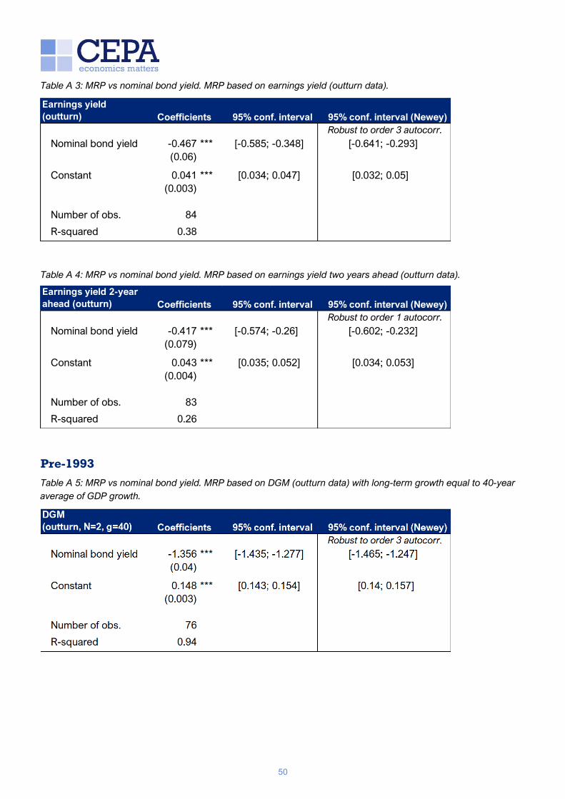
50
Table A 3: MRP vs nominal bond yield. MRP based on earnings yield (outturn data).
Table A 4: MRP vs nominal bond yield. MRP based on earnings yield two years ahead (outturn data).
Pre-1993
Table A 5: MRP vs nominal bond yield. MRP based on DGM (outturn data) with long-term growth equal to 40-year
average of GDP growth.
Earnings yield
(outturn) Coefficients 95% conf. interval 95% conf. interval (Newey)
Robust to order 3 autocorr.
Nominal bond yield -0.467 *** [-0.585; -0.348] [-0.641; -0.293]
(0.06)
Constant 0.041 *** [0.034; 0.047] [0.032; 0.05]
(0.003)
Number of obs. 84
R-squared 0.38
Earnings yield 2-year
ahead (outturn) Coefficients 95% conf. interval 95% conf. interval (Newey)
Robust to order 1 autocorr.
Nominal bond yield -0.417 *** [-0.574; -0.26] [-0.602; -0.232]
(0.079)
Constant 0.043 *** [0.035; 0.052] [0.034; 0.053]
(0.004)
Number of obs. 83
R-squared 0.26

51
Table A 6: MRP vs nominal bond yield. MRP based on DGM (outturn data) with long-term growth equal to 5-year
average of GDP growth.
Table A 7: MRP vs nominal bond yield. MRP based on earnings yield (outturn data).
Table A 8: MRP vs nominal bond yield. MRP based on earnings yield two years ahead (outturn data).
Earnings yield
(outturn) Coefficients 95% conf. interval 95% conf. interval (Newey)
Robust to order 3 autocorr.
Nominal bond yield -0.451 *** [-0.582; -0.32] [-0.648; -0.254]
(0.065)
Constant 0.042 *** [0.034; 0.05] [0.03; 0.058]
(0.004)
Number of obs. 57
R-squared 0.37
Earnings yield 2-year
ahead (outturn) Coefficients 95% conf. interval 95% conf. interval (Newey)
Robust to order 1 autocorr.
Nominal bond yield -0.408 *** [-0.58; -0.236] [-0.611; -0.204]
(0.086)
Constant 0.046 *** [0.036; 0.056] [0.033; 0.058]
(0.005)
Number of obs. 58
R-squared 0.26

52
Post-1993
Table A 9: MRP vs nominal bond yield. MRP based on DGM (outturn data) with long-term growth equal to 40-year
average of GDP growth.
Table A 10: MRP vs nominal bond yield. MRP based on DGM (outturn data) with long-term growth equal to 5-year
average of GDP growth.
Table A 11: MRP vs nominal bond yield. MRP based on earnings yield (outturn data).
Earnings yield
(outturn) Coefficients 95% conf. interval 95% conf. interval (Newey)
Nominal bond yield -0.883 *** [-1.092; -0.674] NA
(0.101)
Constant 0.056 *** [0.043; 0.068] NA
(0.006)
Number of obs. 27
R-squared 0.75

53
Table A 12: MRP vs nominal bond yield. MRP based on earnings yield two years ahead (outturn data).
REGRESSION RESULTS – FORECAST DATA
Whole sample
Table A 13: MRP vs nominal bond yield. MRP based on DGM (forecast data) with long-term growth based on IMF
forecasts.
Table A 14: MRP vs nominal bond yield. MRP based on earnings yield (forecast data).
Earnings yield 2-year
ahead (outturn) Coefficients 95% conf. interval 95% conf. interval (Newey)
Nominal bond yield -0.878 *** [-1.085; -0.671] NA
(0.1)
Constant 0.060 *** [0.048; 0.072] NA
(0.006)
Number of obs. 25
R-squared 0.71

54
INDEPENDENT EXPERT REPORTS REVIEWED
Target Expert MRP Date Evidence Risk-free rate
Focus
minerals
BDO 6-
8%
19 March
2013
• Capital
weighted
average of
ASX sample
minus risk-
free rate.
• Spot YTM
10-year
government
bond.
Blackwood Grant
Thornton
6% 26
November
2013
• Empirical
studies.
• Consistent
with
regulators
(ACCC and
other state
based
regulators).
• 5-year
average of
10-year
government
bond
yields.
Aquila
Resources
Grant
Samuel
6% 20 June
2014
• Long run
historical
data.
• Consistent
with other
analysts.
• Spot YTM
10-year
government
bond.
Gondwana
Resources
BDO 6-
8%
18 July
2014
• Capital
weighted
average of
ASX sample
minus risk-
free rate.
• Spot YTM
10-year
government
bond.
Country
Road
Lonergan
Edwards
6% 21 July
2014
• Consistent
with
empirical
studies, other
valuation
reports and
regulatory
precedent.
• 50 basis
points
higher than
spot TYM
of 20-year
government
bonds.118
Phoenix Gold BDO 6-
8%
3
September
2015
• Capital
weighted
average of
ASX sample
minus risk-
free rate.
• Spot YTM
10-year
government
bond.
Devine KPMG 6% 10
December
2015
• Consistent
with other
valuation
reports.
• Spot YTM
and long-
term
forecasts
on 10-year
———————————————————————————————————————————————————
118 This is due to their belief that current rates are unsustainably low.

55
Target Expert MRP Date Evidence Risk-free rate
government
bond.
Ethane
Pipeline
Income Fund
Lonergan
Edwards
6% 1 April 2016 • Empirical
studies
• Australian
regulators
• Other
valuation
reports
• 90 basis
points
higher than
spot TYM
of 20-year
government
bonds.119
UGL Limited Grant
Samuel
6% 7 November
2016
• Long run
historical
data.
• Consistent
with other
analysts.
• Spot YTM
10-year
government
bond.
CIMIC Group Lonergan
Edwards
6% 27 February
2017
• Historical
excess
returns.
• AER.
• Fernandez
survey.
• 20 basis
points
higher than
spot TYM
of 30-year
government
bonds.120
Lepidico BDO 6-
8%
28 March
2017
• Capital
weighted
average of
ASX sample
minus risk-
free rate.
• Spot YTM
10-year
government
bond.
AWE Limited Grant
Thornton
6% 21 February
2018
• Long run
historical
analysis.
• 10-year
average of
10-year
government
bond
yields.
Integral
Diagnostics
Lonergan
Edwards
6% 2 March
2018
• N/A • 60 basis
points
higher than
spot TYM
of 30-year
government
bonds.121
Primary Gold BDO 6-
8%
21 March
2018
• Capital
weighted
average of
ASX sample
• Spot YTM
3-year
government
bond.
———————————————————————————————————————————————————
119 This is due to their belief that current rates are unsustainably low.
120 This is due to their belief that current rates are unsustainably low.
121 This is due to their belief that current rates are unsustainably low.

56
Target Expert MRP Date Evidence Risk-free rate
minus risk-
free rate.
Atlas Irons BDO 6-
8%
16 July
2018
• Capital
weighted
average of
ASX sample
minus risk-
free rate.
• Spot YTM
2-year
government
bond.
Tilt
Renewables
Grant
Thornton
6% 25
September
2018
• Long run
historical
analysis.
• Consistent
with
regulators.
• Long term
yield on 10-
year
government
bonds.
Stanmore
Coal
BDO 6% 12
December
2018
• N/A • Spot YTM
15-year
government
bond.
AHG Limited KPMG 6% 16 May
2019
• N/A • Blend of
spot rate
YTM and
long-term
average.
Alliance
Resources
FTI 6% 10
September
2019
• N/A • Spot YTM
5-year
government
bond.
Macquarie
Media
PWC 6% 13
September
2019
• N/A • N/A
Stanmore
Coal
BDO 6% 29 April
2020
• N/A • 14 day
average on
15-year
government
bonds.
Australian
Power and
Gas
Company
Limited
Grant
Thornton
6% 23 August
2020
• Empirical
studies.
• Consistent
with regulators
(ACCC and
other state
based
regulators).
• 10 day
average on
10-year
government
bonds.
Spotless Deloitte 8.3% 1
September
2020
• N/A • 5 day
average of
zero
coupon 10-
year
government
bonds.

57
EXPERT WITNESS COMPLIANCE
I have read the Federal Court’s “Expert Evidence Practice Note” as published 25th October 2016. This report has
been prepared in accordance with the practice note and I agree to be bound by it. This report is based wholly or
substantially on specialised knowledge that has arisen from my training, study and experience and I attach my
qualifications below. In coming to my conclusions, I have made all the inquiries I believe are desirable and
appropriate and no matters of significance that I regard as relevant have, to my knowledge, been withheld from the
Court. This report was prepared to answer a set of questions asked by the Commonwealth of Australia (as
represented by the Australian Competition & Consumer Commission) and I also attach a copy of their instructions
below. I was assisted in my examinations by Benjamin Osenius-Eite, Tommaso Autorino and Jacob Peyton and
attach their qualifications below.
Signed
Jonathan Mirrlees-Black
58
CURRICULUM VITAE
Jonathan Mirrlees-Black
Summary of experience
Jonathan has over 30 years of experience as an economist and finance professional in infrastructure, as a sell-
side and buy-side investment analyst and as an advisor to global infrastructure companies, regulators,
international organisations, and private equity investors. He is a Director of CEPA’s Sydney office and has
directed cost of capital projects for a wide range of clients in Australian, New Zealand, UK and other jurisdictions.
From 2010-15 he was Senior Advisor then Head of Research at RARE Infrastructure, a Sydney-based specialist
investor in global listed infrastructure (energy networks, water, roads, rail, ports, airports, and communications
infrastructure) with a long-term value-based investment approach.
Selected recent project experience
• Australia: Use of infrastructure in recovery from COVID-19 Crisis, Global Infrastructure Hub, 2020
• Australia, Review of Port of Melbourne’s Rate of Return Methodology & Calculations, Essential Services
Commission (ESC), 2020
• Australia: due diligence for infrastructure asset, confidential client, 2019
• Australia: due diligence for infrastructure asset, confidential client, 2018
• Australia: advice on macroeconomics to an infrastructure fund, 2018-ongoing
• Australia: Chair of Investment Advisory Board (IAB), RARE Infrastructure, 2010-15
• UK, cost of capital and regulatory finance advice, Ofgem, 2019-20
• Ireland, cost of capital and regulatory finance advice, CER, 2019-20
• UK, cost of capital and regulatory finance advice, IAG, 2019-20
• UK, review of debt beta, UK Regulator’s Network, 2019
• New Zealand: Asset beta, leverage and credit rating, New Zealand Commerce Commission, 2019
• Malaysia: Weighted average cost of capital for a Malaysian Utility, TNB, 2019
• New Zealand: Asset beta in the dairy industry, New Zealand Commerce Commission, 2019.
• Malaysia: Weighted average cost of capital for a Malaysian Utility, Confidential, 2019
• Australia: Facilitator for expert evidence sessions, AER, 2018
• New Zealand. Asset beta in the dairy industry. New Zealand Commerce Commission, 2018.
• Australia: Inflation expectations, Energy Networks Australia, 2017
• Malaysia: Weighted average cost of capital for TNB, Tenaga Nasional Berhad, 2016-17
• New Zealand: Advice on cost of capital, New Zealand Commerce Commission, 2016
• UK: advice to CAA and Ofwat on the cost of debt, 2016
• UK: Regulatory advice, Heathrow Airport Operators Committee (AOC), 2013-2014
• Australia: Cost of capital for global listed infrastructure companies, RARE Infrastructure 2011-15
• Australia: Integrated System Plan (ISP) Financeability, AEMC, 2020-2021
• Australia: review of regimes for water regulation, IPART, 2020
• Australia: Incentives for capital investment, AEMC, 2018
• Australia: Coordination of generation and transmission investment, AEMC 2017-18
• Australia: Contestability of energy services. AEMC, 2016.
• Australia: Future regulatory options for electricity networks, ENA and CSIRO, 2016
• Australia: Assessing demand forecasting approaches, CitiPower / Powercor, 2016
• Australia: Efficiency sharing schemes, IPART, 2016
• Australia: Governance of market and system operators, Australian Energy Council and Energy Networks
Australia, 2020
• Australia: Regulation of energy markets. Australian regulatory authority, 2017

59
• Australia: energy market aggregator business planning, 2016
• Australia: Transition mechanisms for the reform of the Victorian Declared Wholesale Gas Market, The
Australian Energy Market Commission, 2016
• Australia: Sea Ports Research, RARE Infrastructure, 2011-15
• New Zealand: Fibre Regulation - Commerce Commission, 2018
Qualifications and training
1999 University of Oxford (St. John’s College), D.Phil. Economics
1987 University of Oxford (St. John’s College), M.Phil. Economics
1985 University of Sheffield, B.A. Pure Mathematics, First Class Honours
2013
2020
Fellow, Australian Institute of Energy
Member, Australian Institute of Company Directors
Employment history
2016 – Present Director, CEPA, Sydney, Australia
2013 – 2020 Honorary Professor / Visiting Professor, University College London
2011 – 2015 Head of Research, Chair of Investment Advisory Board, RARE Infrastructure, Sydney, Australia
2010 – 2011 Senior Advisor, Member of Investment Advisory Board, RARE Infrastructure, Sydney, Australia
2009 – 2015 Senior Advisor, CEPA
2004 – 2009 Head of Utilities Research (2004-07), Cross-sector analyst (2007-09), Exane BNP Paribas,
London, UK
2003 – 2004 Director, CEPA, London, UK
1999 – 2002 Executive Director, Head of European Utilities Research, Lehman Brothers, London, UK
1996 – 1999 Director, European Utilities Analyst, Dresdner Kleinwort Benson, London, UK
1995 – 1996 Assistant Director, European Utilities Research, Union Bank of Switzerland, London, UK
1990 – 1995 Principal Associate, Coopers & Lybrand, London, UK
1988 – 1990 Analyst, Corporate Planning, British Petroleum Company, London, UK
1986 – 1988 Lecturer in Economics, Exeter College Oxford, UK

60
Benjamin Osenius-Eite
Summary of experience
At CEPA he has contributed to several projects in the energy and infrastructure space focusing on regulated
utilities. This has included projects on cost of capital estimation and regulatory reform of access and pricing.
Prior to joining CEPA Australia he worked at the Department for Transport in the UK as an Economic Adviser on
EU Exit. Here he led a team examining transport impacts from potential changes at key UK ports. During his time
at the NAO he delivered a range of value for money studies with a focus on the health sector examining the
effectiveness of government expenditure. Before this Benjamin worked on the regulation of retail financial
products at HM Treasury in the UK.
Between 2012-2014 Benjamin was posted as an ODI Fellow to Vanuatu’s Ministry of Finance and Economic
Management. He advised the Vanuatu government on the effective use of funds in the health sector.
Selected project experience
• Malaysia: Weighted average cost of capital estimates and regulatory advice, TNB, 2019-2021
• Australia: Review of Port of Melbourne’s Rate of Return Methodology & Calculations, Essential Services
Commission (ESC), 2020
• Pacific Islands: Review of Global Investment Platforms, IFC (World Bank Group), 2020
• Australia: Governance of market and system operators, Australian Energy Council and Energy Networks
Australia, 2020
• Global: Post-COVID-19 economic recovery through infrastructure, Global Infrastructure Hub, 2020
• Australia: Economic regulation of water utilities – research, IPART, 2020
• UK, Ofgem, Time Value of Money, 2020.
• Singapore: Demand Side Management Review, Energy Market Authority, 2020.
• Australia: Access and pricing, Australian Energy Market Commission, 2020
• Australia: Review of Return Review, Queensland Competition Authority (QCA), 2020-2021
• Australia: Advice on an appropriate asset beta and other WACC parameters for GAWB 2020-2025,
Queensland Competition Authority (QCA), 2019-2020
• Ireland: Economic and Technical Consultancy Services to Review and Assess Electricity Interconnectors
Applications, CRU, 2019
• New Zealand: Asset beta, leverage and credit rating, New Zealand Commerce Commission, 2019
Qualifications and training
2012 MSc Development Economics (Merit), SOAS, University of London, London, United Kingdom
2011 BSc (Hons) Economics (2:1), SOAS, University of London, London, United Kingdom
Countries of experience
United Kingdom, Ireland, Singapore, Australia, Malaysia, Vanuatu
Employment history
2019 - Present Senior Consultant, CEPA, Sydney, Australia
2018-2019 Economic Adviser, EU Exit Transport Analysis, Department for Transport, HM Government,
United Kingdom
2015-2018 Analyst, Health Value for Money, National Audit Office, United Kingdom
2015-2015 Policy Advisor, Assets, Savings and Consumers, HM Treasury, HM Government, United
Kingdom
2012-2014 Expenditure Analyst, Overseas Development Institute / Ministry of Finance and Economic
Management, Port Vila, Vanuatu

61
Tommaso Autorino
Summary of experience
Tommaso joined CEPA in 2018. His key areas of expertise include economic regulation, regulatory finance, and
pricing arrangements in the energy, communications, and transport sectors.
Tommaso advises regulators in Australia and New Zealand on various components of the Weighted Average
Cost of Capital (WACC), including asset beta, leverage, and market risk premium. His experience also includes
developing financial and econometric models for use in both commercial and regulatory settings.
Selected project experience
• Australia: Advice on the financeability of Integrated System Plan (ISP) projects, Australian Energy Market
Commission (AEMC), 2021
• Australia: Review of Port of Melbourne’s Rate of Return Methodology & Calculations, Essential Services
Commission (ESC), 2020
• Australia: Distributed Energy Resources Integration Program (DEIP) – Access and Pricing, AEMC, 2020
• New Zealand: Advice on Weighted Average Cost of Capital, NZCC, 2019-2020
• Great Britain: RIIO-2 gas distribution price control, Ofgem, 2019-2020
• Australia: Research on best practice utility regulation, IPART, 2020
• Australia: Workshop on AER’s benchmarking and use of RIN data, Confidential client, 2019-2020
• Australia: Governance of market and system operators, Australian Energy Council and Energy Networks
Australia, 2020
• Australia: Due diligence for infrastructure asset, Confidential client, 2019
• Ireland: Network tariffs review, EirGrid, 2019
• Australia: Network pricing reform, Energy Networks Australia, 2019
• Australia: Customer engagement review, Sydney Water, 2019
• Ireland: Review of track access charges, Irish Rail Essential Functions Body (EFB), 2019
Qualifications and training
2017 Master in Economic and Social Sciences, Bocconi University, Milan, Italy
2014 Bachelor of Economics, University of Tor Vergata, Rome, Italy
Employment history
2018 – present Consultant, CEPA, Sydney, Australia
2017 Credit Analyst, REV, Rome, Italy
2016 Research Intern, United Nations Joint Inspection Unit, Geneva, Switzerland

62
Jacob Peyton
Summary of experience
Jacob joined CEPA in 2021. Prior to joining CEPA Australia he worked as an economist for the New Zealand
Commerce Commission. Here he provided economic advice assessing the impact on competition of merger and
acquisitions, in particular the Knauf USG Boral merger and the Cengage McGraw-Hill merger.
Before joining the New Zealand Commerce Commission Jacob worked as a reporter for leading private news
agency Select Committee News and tutored finance and economics at Victoria University of Wellington.
Selected project experience
• New Zealand: Support for implementation of fibre regulation, New Zealand Commerce Commission (NZCC),
2021 - ongoing
• Grocery Sector Market Study, New Zealand Commerce Commission, 2021.
• Motor Vehicle add-on Insurance, New Zealand Commerce Commission, 2020-2021.
• Glenninburgh Holdings and Wallace Group Section 47 Investigation, New Zealand Commerce Commission,
2020-2021.
• Heyden Farms Limited, Henergy Cage-Free Limited and Rasmusens Poultry Farms Limited Merger
Application, New Zealand Commerce Commission, 2020.
• Cengage McGraw-Hill Merger Application, New Zealand Commerce Commission, 2019-2020.
• Retail Fuel Market Study, New Zealand Commerce Commission, 2019.
• Knauf USG Boral Merger Application, New Zealand Commerce Commission, 2018-2019.
• Fletcher Building and Waikato Aggregates Limited Merger Application, New Zealand Commerce Commission,
2018.
• Infant Nutrition Council Authorisation, New Zealand Commerce Commission, 2018.
• Wilson Parking Section 47 Commerce Act Investigation, New Zealand Commerce Commission, 2017-2018.
Qualifications and training
2018-2020
2017
Passed level I and level II CFA exam.
Mcom Finance, Victoria University of Wellington, Wellington, New Zealand.
2016 Bcom (Hons) Finance & Economics, Victoria University of Wellington, Wellington, New Zealand.
Employment history
2021 - Present Consultant, CEPA, Sydney, Australia
2017-2021 Economist, New Zealand Commerce Commission, Wellington, New Zealand

63
TERMS OF REFERENCE
Background
The AER applies a ‘building block’ model to set regulated revenues for electricity and gas network service
providers. The building blocks—return on capital, return of capital, operating expenditure and tax —reflect the
expected costs that would be incurred by a benchmark efficient entity operating the network. This is a form of
incentive regulation, as building blocks are estimated in advance for a regulatory control period (typically five years)
and the networks retain any benefit (or bears any detriment) where it is able to reduce costs below the AER’s
estimates. Revealed costs are then used to inform building block estimates for the following control period, so that
efficiency gains are passed on to consumers. The AER also operates a number of incentive schemes in conjunction
with the building block framework.
The return on capital building block is set by applying a rate of return on capital to the regulatory asset base (RAB)
each year. The AER estimates the allowed rate of return for regulated businesses using the approach set out in the
2018 RoR Instrument. The Rate of Return Instrument is binding under the National Electricity Law and National Gas
Law. This means that the AER and network businesses are required to set the rate of return according to the
current Instrument. There is a four year cycle for the development of the next rate of return instrument (the 2022
instrument), which is to be published in December 2022.
The 2022 instrument is to be developed through a comprehensive consultation process, with consumers, investors
and businesses included throughout the process. The AER has already commenced its ‘Pathway to 2022’ work
program for the development of the 2022 instrument. The AER must be satisfied that the approach to setting the
allowed rate of return achieves the National Electricity Objective (NEO) and National Gas Objective (NGO), and the
related revenue and pricing principles (RPPs).
While the 2022 Instrument does not have to adopt the 2018 approaches, the 2018 RoR Instrument applies the
following key characteristics when estimating a businesses’ allowed rate of return:
• It use a nominal vanilla weighted average cost of capital (WACC) formulation (used in a post-tax revenue
model, i.e. effect of the interest tax shield is considered in cashflows)
• It assumes a 40% equity and 60% debt capital structure.
• It uses a domestic Capital Asset Pricing Model (CAPM) to estimate the Return on Equity (RoE). This is
estimated as:
o The risk free rate is estimated from the yield on 10 year to maturity Commonwealth Government
Securities (CGS) over a short averaging period prior to the commencement of the regulatory control
period (between 20 and 60 business days).
o Equity beta of 0.6 (fixed for the life of the 2018 instrument)
o Market risk premium of 6.1 per cent (also fixed for the life of the 2018 instrument)
o This means the RoE is the risk free rate plus a fixed premium of 3.66%.
• It uses a trailing average portfolio for the allowed return on debt, updating 10% of the portfolio estimate
annually (i.e. a ten year rolling window of annual return on debt observations).
• Annual return on debt are based on debt costs for the benchmark BBB+ credit rating at a 10 year term,
estimated by weighting A rated and BBB rated benchmark curves (from a number of providers) over an
averaging period.
• Market data for the return on debt and risk free rate is sourced from averaging periods nominated by the
network businesses in advance.
• It uses a gamma (assumed utilisation of imputation credits) value of 0.585, fixed for the life of the 2018
instrument.
The focus of this request for quote is to explore:
• Whether any relationship between the risk-free rate (RFR) and market risk premium (MRP) can be
identified with sufficient certainty and specificity for use when estimating the return on equity; and
• the merits or otherwise of using any relationship found between the RFR and the MRP when estimating the
required return on equity.

64
Project scope
Summary
The AER seeks advice on the return on equity approach for use in the AER’s regulatory framework to determine the
regulated rate of return that meets its legislated objectives—that is, setting a return on capital building block that
achieves the NEO and NGO. This means our rate of return instrument should promote—to the greatest degree—
efficient investment in, and efficient operation and use of, electricity or gas network services for the long term
interests of consumers. We consider efficient financing costs are reflected in the prevailing market cost of capital
(or WACC) for an investment with a similar degree of risk as that which applies to a service provider in respect of
the provision of regulated services.
The AER requires an expert advisor to explore whether the market risk premium (MRP) varies through time and, if
so, whether changes are correlated with changes in the risk-free rate of interest (RFR). To the extent that a
relationship with the RFR can be identified, the expert is required to advise us on how we might reflect this in our
2022 Instrument. At this point we are seeking a high level review of the key evidence and options we might
consider for reflecting any relationship (if identified). The advice does not need to comprehensively explore every
detail of the issue. We will publish the advice alongside a draft working paper which will allow us to explore the
issue further with stakeholders and help us develop initial views.
The expert advisor is requested to use the following criteria when evaluating the approach or any additional models
for use in the regulatory framework (noting the overarching objective is to estimate a return on equity that will
contribute to the achievement of the NEO and NGO):
• Reliability—produces estimates of the return on equity that reflect economic and finance principles,
empirical evidence, and market information; estimates have minimal error, and are free from bias.
• Relevance to the Australian benchmark—as the benchmark firm operates in Australia; this may include
ability to populate the model with Australian-relevant data.
• Suitability for use in regulated environment—this may include transparency, replicability, and consideration
of any incentive effects.
• Simplicity–avoids unnecessary complexity or spurious precision, is able to be understood by a broad
stakeholder set.
The expert may adopt alternative (or additional) criteria, though it should explain why it has adopted these criteria if
so.
The expert advisor is requested to consider:
• Key relevant academic literature on the cost of capital
• Methodologies adopted by overseas regulators for example Ofgem, namely the ‘Wright’ approach (also
called the Total Market Returns Approach), and the Federal Energy Regulatory Commission (FERC)
• Practice in financial markets, including (but not restricted to):
o approaches used by institutional investors
o valuation techniques used by equity brokers/analysts.
The expert should also be familiar with the following background documents (available on the AER website):
• the 2018 RoR Instrument
• the 2018 RoR Instrument final explanatory statement, particularly:
o section 1.3 sets out the AER’s position on the content for the next review
o section 5 sets out the AER’s framework for setting the return on equity
o section 5.2.5.1 sets out the regard had to the Wright approach in informing the overall return on equity
o section 5.4.5.5 sets out the different methodology’s used by international regulators.
o section 9.2.2 sets out other regulators decisions
o section 9.2.4 sets out AER’s position on the relationship between the market with the risk free rate
• an assessment by Associate Professor Graham Partington and Professor Stephen Satchell on submissions
to the draft 20218 ROR Instrument explanatory statement
65
The key deliverable is a written report that includes:
• An introductory section:
o outlining the assessment work undertaken by the expert
o describing the criteria used to assess any approach or model that might be used to explain the MRP
and any relationship it has with the the RFR
o summarising any important developments in academic literature on any observed or theorised
relationship between the RFR and the MRP (or lack of a relationship).
• A section that discusses the practical and theoretical basis for any possible relationship. This should
include:
o An assessment of whether the MRP moves through time
o Consideration of whether any relationship with the RFR estimated is likely to be genuine, robust and
stable through time
o Why the required return on equity may move more (or less) than the promised yields on long term
investment grade corporate debt with regard to movements in the long term Commonwealth
Government bond yields.
o If movements in the promised yields through time on long term investment grade corporate debt
relative to the Commonwealth Government bond yields appear to support (or refute) any potential
relationship and provide any evidence on its likely stability.
• For the methodologies adopted by overseas regulators:
o A brief summary of how they are used; the justification for their adoption, and how robust the empirical
evidence and theoretical justifications appears to be for their use.
o Your own assessment of any basis for the approaches in terms of finance theory (academic literature),
empirical evidence and financial market practice.
o An evaluation of the strengths and weakness of these approaches in the Australian domestic market
context, including in relative terms against any other models the expert has considered.
o Reviewing approaches employed by overseas regulators could be a large, time consuming task. In the
first instance we are seeking a high level assessment only. We direct to the consultant to work already
undertaken by the Brattle Group for the AER . The consultant may also draw on any material readily at
hand.
• A recommendation on:
o The merits or otherwise of whether a relationship between the RFR and MRP can be identified for the
Australian domestic market.
o To the extent that there is a relationship, how could we reflect this is in the 2022 Instrument
o The key reasoning supporting these recommendations
o Any limitations or requirements for further work
The report is to be written to the standard of the Federal Court Guidelines for Expert Witnesses, and the AER is to
be provided an opportunity to comment on the draft report.

UK
Queens House
55-56 Lincoln’s Inn Fields
London WC2A 3LJ
T. +44 (0)20 7269 0210
www.cepa.co.uk
Australia
Level 20, Tower 2 Darling Park
201 Sussex St
Sydney NSW2000
T. +61 2 9006 1307
www.cepa.net.au