Embed Size (px)
Citation preview

Reinforcement Learning: A Brief Tutorial
Doina PrecupReasoning and Learning Lab
McGill University
http://www.cs.mcgill.ca/∼dprecup
With thanks to Rich Sutton

Outline
• The reinforcement learning problem
• Markov Decision Processes
• What to learn: policies and value functions
• Dynamic programming methods
• Temporal-difference learning methods
• Some interesting, open research problems
September 2005 2 Reinforcement learning: A brief tutorial
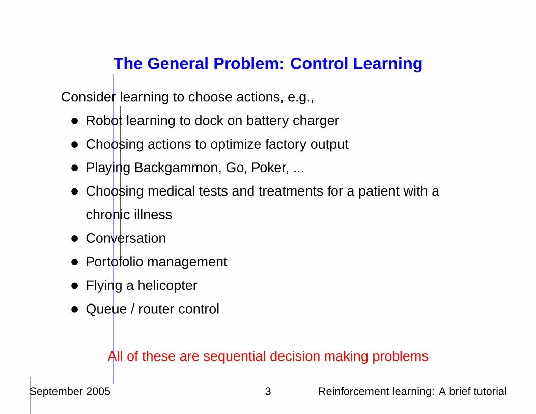
The General Problem: Control Learning
Consider learning to choose actions, e.g.,
• Robot learning to dock on battery charger
• Choosing actions to optimize factory output
• Playing Backgammon, Go, Poker, ...
• Choosing medical tests and treatments for a patient with a
chronic illness
• Conversation
• Portofolio management
• Flying a helicopter
• Queue / router control
All of these are sequential decision making problems
September 2005 3 Reinforcement learning: A brief tutorial

Reinforcement Learning Problem
Agent
Environment
actionatst
rewardrt
rt+1
st+1
state
• At each discrete time t, the agent (learning system) observes
state st ∈ S and chooses action at ∈ A
• Then it receives an immediate reward rt+1 and the state
changes to st+1
September 2005 4 Reinforcement learning: A brief tutorial

Example: Backgammon (Tesauro, 1992-1995)
white pieces move counterclockwise
1 2 3 4 5 6 7 8 9 10 11 12
18 17 16 15 14 13192021222324
black pieces move clockwise
• The states are board positions in which the agent can move
• The actions are the possible moves
• Reward is 0 until the end of the game, when it is ±1 depending
on whether the agent wins or loses
September 2005 5 Reinforcement learning: A brief tutorial

Key Features of RL
• The learner is not told what actions to take, instead it find finds
out what to do by trial-and-error search
• The environment is stochastic
• The reward may be delayed, so the learner may need to
sacrifice short-term gains for greater long-term gains
• The learner has to balance the need to explore its environment
and the need to exploit its current knowledge
September 2005 6 Reinforcement learning: A brief tutorial

The Power of Learning from Experience
• Expert examples are expensive and scarce
• Experience is cheap and plentiful!
September 2005 7 Reinforcement learning: A brief tutorial

Markov Decision Processes (MDPs)
• Set of states S
• Set of actions A(s) available in each state s
• Markov assumption: st+1 and rt+1 depend only on st, at and
not on anything that happened before t
• Rewards:
ra
ss′ = E˘
rt+1|st = s, at = a, st+1 = s′¯
• Transition probabilities
pa
ss′ = P`
st+1 = s′|st = s, at = a
´
September 2005 8 Reinforcement learning: A brief tutorial

Agent’s Learning Task
Execute actions in environment, observe results, and learn policy
(strategy, way of behaving) π : S ×A→ [0, 1],
π(s, a) = P (at = a|st = s)
If the policy is deterministic, we will write it more simply as
π : S → A, with π(s) = a giving the action chosen in state s.
• Note that the target function is π : S → A but we have
no training examples of form 〈s, a〉
Training examples are of form 〈〈s, a〉, r, s′, . . . 〉
• Reinforcement learning methods specify how the agent should
change the policy as a function of the rewards received over
time
September 2005 9 Reinforcement learning: A brief tutorial

The Objective: Maximize Long-Term Return
Suppose the sequence of rewards received after time step t is
rt+1, rt+2 . . . . We want to maximize the expected return E{Rt}
for every time step t
• Episodic tasks: the interaction with the environment takes placein episodes (e.g. games, trips through a maze etc)
Rt = rt+1 + rt+2 + · · ·+ rT
where T is the time when a terminal state is reached
September 2005 10 Reinforcement learning: A brief tutorial

The Objective: Maximize Long-Term Return
Suppose the sequence of rewards received after time step t is
rt+1, rt+2 . . . . We want to maximize the expected return E{Rt}
for every time step t
• Discounted continuing tasks :
Rt = rt+1 + γrt+2 + γ2rt+3 + · · · =
∞X
k=1
γt+k−1rt+k
where γ is a discount factor for later rewards (between 0 and 1,
usually close to 1)
The discount factor is sometimes viewed as an ”inflation rate” or
”probability of dying”
September 2005 11 Reinforcement learning: A brief tutorial

The Objective: Maximize Long-Term Return
Suppose the sequence of rewards received after time step t is
rt+1, rt+2 . . . . We want to maximize the expected return E{Rt}
for every time step t
• Average-reward tasks:
Rt = limT→∞
1
T(rt+1 + rt+2 + · · ·+ rT )
September 2005 12 Reinforcement learning: A brief tutorial

Example: Pole Balancing
Avoid failure: pole falling beyond a given angle, or cart hitting the
end of the track
• Episodic task formulation: reward = +1 for each step before
failure
⇒ return = number of steps before failure
• Continuing task formulation: reward = -1 upon failure, 0
otherwise, γ < 1
⇒ return = −γk if there are k steps before failure
September 2005 13 Reinforcement learning: A brief tutorial

Example: Pole Balancing
Avoid failure: pole falling beyond a given angle, or cart hitting the
end of the track
• Episodic task formulation: reward = +1 for each step before
failure
⇒ return = number of steps before failure
• Discounted continuing task formulation: reward = -1 upon
failure, 0 otherwise, γ < 1
⇒ return = −γk if there are k steps before failure
September 2005 14 Reinforcement learning: A brief tutorial
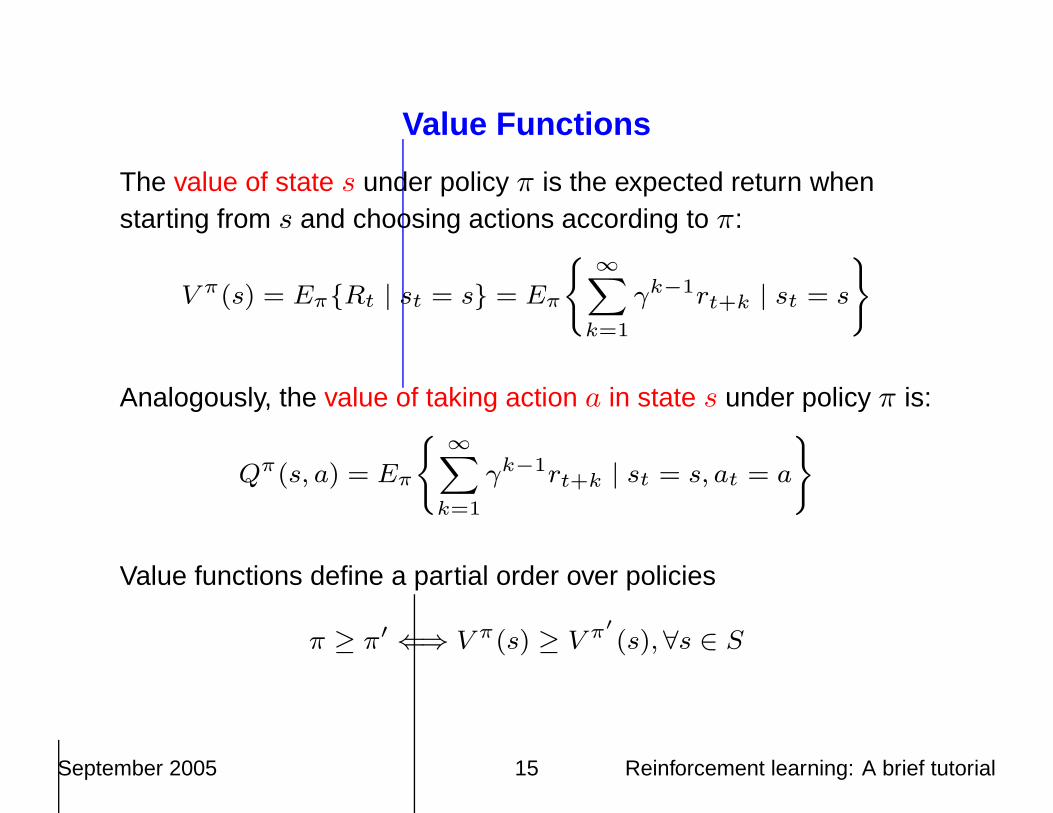
Value Functions
The value of state s under policy π is the expected return whenstarting from s and choosing actions according to π:
V π(s) = Eπ{Rt | st = s} = Eπ
(
∞X
k=1
γk−1rt+k | st = s
)
Analogously, the value of taking action a in state s under policy π is:
Qπ(s, a) = Eπ
(
∞X
k=1
γk−1rt+k | st = s, at = a
)
Value functions define a partial order over policies
π ≥ π′ ⇐⇒ V π(s) ≥ V π′
(s),∀s ∈ S
September 2005 15 Reinforcement learning: A brief tutorial

Optimal Policies and Optimal Value Functions
• In an MDP, there is a a unique optimal value function:
V ∗(s) = maxπ
V π(s)
This result was proved by Bellman in the 1950s
• There is also at least one deterministic optimal policy:
π∗ = arg max
πV
π
It is obtained by greedily choosing the action with the best value
at each state
• Note that value functions are measures of long-term
performance, so the greedy choice is not myopic
September 2005 16 Reinforcement learning: A brief tutorial

Markov Decision Processes
• A general framework for non-linear optimal control, extensively
studied since the 1950s
• In optimal control
– Specializes to Ricati equations for linear systems
– Hamilton-Jacobi-Bellman equations for continuous-time
• In operations research
– Planning, scheduling, logistics, inventory control
– Sequential design of experiments
– Finance, marketing, queuing and telecommunications
• In artificial intelligence (last 15 years)
– Probabilistic planning
• Dynamic programming is the dominant solution method
September 2005 17 Reinforcement learning: A brief tutorial

Bellman EquationsValues can be written in terms of successor values
E.g. Vπ(s) = Eπ
˘
rt+1 + γrt+2 + γ2rt+3 + · · · | st = s
¯
= Eπ{rt+1 + γV (st+1) | st = s}
=X
a∈A
π(s, a)X
s′∈S
pa
ss′
`
ra
ss′ + γVπ(s′)
´
This is a system of linear equations whose unique solution is V π .
Bellman optimality equations for the value of the optimal policy:
V∗(s) = max
a∈A
X
s′∈S
pa
ss′
`
ra
ss′ + γV∗(s′)
´
This produces a nonlinear system, but still with a unique solution
September 2005 18 Reinforcement learning: A brief tutorial

Dynamic Programming
Main idea: turn Bellman equations into an update rules.
For instance, value iteration approximates the optimal value function
by doing repeated sweeps through the states:
1. Start with some initial guess, e.g. V0
2. Repeat:
Vk+1(s)← maxa∈A
X
s′∈S
pa
ss′
`
ra
ss′ + γVk(s′)´
3. Stop when the maximum change between two iterations is
smaller than a desired threshold (the values stop changing)
In the limit of k →∞, Vk → V ∗, and any of the maximizing actions
will be optimal.
September 2005 19 Reinforcement learning: A brief tutorial

Illustration: Rooms Example
Four actions, fail 30% of the time
No rewards until the goal is reached, γ = 0.9.
Iteration #1 Iteration #2 Iteration #3
September 2005 20 Reinforcement learning: A brief tutorial

Policy Iteration
1. Start with an initial policy π0
2. Repeat:
(a) Compute V πi using policy evaluation
(b) Compute a new policy πi+1 that is greedy with respect to
V πi
until V πi = V πi+1
September 2005 21 Reinforcement learning: A brief tutorial

Generalized Policy Iteration
Any combination of policy evaluation and policy improvement steps,
even if they are not complete
π V
evaluation
improvement
V →Vπ
π→greedy(V)
*Vπ*
September 2005 22 Reinforcement learning: A brief tutorial

Model-Based Reinforcement Learning
• Usually, the model of the environment (rewards and transition
probabilities) is unknown
• Instead, the learner observes transitions in the environment and
learns an approximate model r̂a
ss′, p̂a
ss′
Note that this is a classical machine learning problem!
• Pretend the approximate model is correct and use it to compute
the value function as above
• Very useful approach if the models have intrinsic value, can be
applied to new tasks (e.g. in robotics)
September 2005 23 Reinforcement learning: A brief tutorial

Asynchronous Dynamic Programming
• Updating all states in every sweep may be infeasible for very
large environments
• Some states might be more important than others
• A more efficient idea: repeatedly pick states at random, and
apply a backup, until some convergence criterion is met
• Often states are selected along trajectories experienced by the
agent
• This procedure will naturally emphasize states that are visited
more often, and hence are more important
September 2005 24 Reinforcement learning: A brief tutorial

Dynamic Programming Summary
• In the worst case, scales polynomially in |S| and |A|
• Linear programming solution methods for MDPs also exist, and
have better worst-case bounds, but usually scale worse in
practice
• Dynamic programming is routinely applied to problems with
millions of states
• However, if the model of the environment is unknown,
computing it based on simulations may be difficult
September 2005 25 Reinforcement learning: A brief tutorial

The Curse of Dimensionality
• The number of states grows exponentially with the number of
state variables (the dimensionality of the problem)
• To solve large problems:
– We need to sample the states
– Values have to be generalized to unseen states using
function approximation
September 2005 26 Reinforcement learning: A brief tutorial

Reinforcement Learning: Using Experience instead of Dynam ics
Consider a trajectory, with actions selected according to policy π:
The Bellman equation is: V π(st) = Eπ [rt+1 + γV π(st+1)|st]
which suggests the dynamic programming update:
V (st)← Eπ [rt+1 + γV (st+1)|st]
In general, we do not know this expected value. But, by choosing
an action according to π, we obtain an unbiased sample of it,
rt+1 + γV (st+1)
In RL, we make an update towards the sample value, e.g. half-way
V (st)←1
2V (st) +
1
2(rt+1 + γV (st+1)
September 2005 27 Reinforcement learning: A brief tutorial

Temporal-Difference (TD) Learning (Sutton, 1988)
We want to update the prediction for the value function based on its
change from one moment to the next, called temporal difference
• Tabular TD(0):
V (st)← V (st)+α (rt+1 + γV (st+1)− V (st)) ∀t = 0, 1, 2, . . .
where α ∈ (0, 1) is a step-size or learning rate parameter
• Gradient-descent TD(0):
If V is represented using a parametric function approximator,
e.g. a neural network, with parameter θ:
θ ← θ+α (rt+1 + γVθ(st+1)− Vθ(st))∇θVθ(st), ∀t = 0, 1, 2, . . .
September 2005 28 Reinforcement learning: A brief tutorial

Eligibility Traces (TD( λ))
δtet etet
et
Time
stst+1
st-1
st-2
st-3
• On every time step t, we compute the TD error:
δt = rt+1 + γV (st+1)− V (st)
• Shout δt backwards to past states
• The strength of your voice decreases with temporal distance by
γλ, where λ ∈ [0, 1] is a parameter
September 2005 29 Reinforcement learning: A brief tutorial

Example: TD-Gammon
Vt+1− Vt
hidden units (40-80)
backgammon position (198 input units)
predicted probabilityof winning, Vt
TD error,
. . . . . .
. . . . . .
. . . . . .
• Start with random network
• Play millions of games against itself
• Value function is learned from this experience using TD learning
• This approach obtained the best player among people and
computers
• Note that classical dynamic programming is not feasible for this
problem!
September 2005 30 Reinforcement learning: A brief tutorial

RL Algorithms for Control
• TD-learning (as above) is used to compute values for a given
policy π
• Control methods aim to find the optimal policy
• In this case, the behavior policy will have to balance two
important tasks:
– Explore the environment in order to get information
– Exploit the existing knowledge, by taking the action that
currently seems best
September 2005 31 Reinforcement learning: A brief tutorial

Exploration
• In order to obtain the optimal solution, the agent must try all
actions
• ǫ-soft policies ensure that each action has at least probability ǫ
of being tried at every step
• Softmax exploration makes action probabilities conditional on
the values of different actions
• More sophisticated methods offer exploration bonuses, in order
to make the data acquisiton more efficient
• This is an area of on-going research...
September 2005 32 Reinforcement learning: A brief tutorial

A Spectrum of Solution Methods
• Value-based RL: use a function approximator to represent the
value function, then use a policy that is based on the current
values
– Sarsa: incremental version of generalized policy iteration
– Q-learning: incremental version of value iteration
• Actor-critic methods: use a function approximator for the value
function and a function approximator to represent the policy
– The value function is the critic, which computes the TD error
signal
– The policy is the actor; its parameters are updated directly
based on the feedback from the critic.
E.g., policy gradient methods
September 2005 33 Reinforcement learning: A brief tutorial

Function Approximation for Value Functions
Many methods from supervised learning have been tried:
• A table where several states are mapped to the same location -
state aggregation
• Gradient-based methods:
– Linear approximators
– Artificial neural networks
– Radial Basis Functions
• Memory-based methods:
– Nearest-neighbor
– Locally weighted regression
• Decision trees
September 2005 34 Reinforcement learning: A brief tutorial

But RL has Special Requirements!
• We need fast, incremental learning (so we can learn during the
interaction)
• As learning progresses, both the input distribution and the
target outputs change!
• So the function approximator must be able to handle
non-stationarity very well.
• As a result, a lot of RL applications use linear or memory-based
approximators.
September 2005 35 Reinforcement learning: A brief tutorial

Sparse, coarse coding
Main idea: we want linear function approximators (because they
have good convergence guarantees) but with lots of features, so
they can represent complex functions
a) Narrow generalization b) Broad generalization c) Asymmetric generalization
• Coarse means that the receptive fields are typically large
• Sparse means that just a few units are active ar any given time
E.g., CMACs, sparse distributed memories etc.
September 2005 36 Reinforcement learning: A brief tutorial

Summary: What RL Algorithms Do
Continual, on-line learning
Many RL methods can be understood as trying to solve the Bellman
optimality equations in an approximate way.
September 2005 37 Reinforcement learning: A brief tutorial

Success Stories
• TD-Gammon (Tesauro, 1992)
• Elevator dispatching (Crites and Barto, 1995): better than industry
standard
• Inventory management (Van Roy et. al): 10-15% improvement over
industry standards
• Job-shop scheduling for NASA space missions (Zhang and Dietterich,
1997)
• Dynamic channel assignment in cellular phones (Singh and Bertsekas,
1994)
• Robotic soccer (Stone et al, Riedmiller et al...)
• Helicopter control (Ng, 2003)
• Modelling neural reward systems (Schultz, Dayan and Montague, 1997)
September 2005 38 Reinforcement learning: A brief tutorial

On-going Research at McGill: Function Approximation
• Theoretical properties
• Learning about many policies simultaneously and efficiently,
from one stream of data; this is called off-policy learning
• How to create a good approximator automatically?
• Practical applications
September 2005 39 Reinforcement learning: A brief tutorial

On-going Research at McGill: Dealing with Partial Observab ility
• In realistic applications, the state of the MDP may not be
perfectly observable.
• Instead, we have noisy sensor readings, or observations
• POMDP model: MDP + a set of observations, and probabilities
of emission from each state
• Unfortunately, since the state is not observable, learning
becomes very difficult (one can use expectation maximization,
but it works poorly in this case)
• We explore:
– Active learning
– Predictive state representations
September 2005 40 Reinforcement learning: A brief tutorial

On-going Research at McGill: Temporal Abstraction
• Planning over courses of actions, called options, rather than just
primitive actions
• The focus is less on optimality and more on modeling the
environment at multiple time scales
• Off-policy learning is crucial for this task
September 2005 41 Reinforcement learning: A brief tutorial

Reference books
• For RL: Sutton & Barto, Reinforcement learning: An introduction
http://www.cs.ualberta.ca/∼sutton/book/the-book.html
• For MDPs: Puterman, Markov Decision Processes
• For theory on RL with function approximation: Bertsekas &
Tsitsiklis, Neuro-dynamic programming
September 2005 42 Reinforcement learning: A brief tutorial

![arXiv:1902.09996v1 [cs.AI] 26 Feb 2019 · 2019. 2. 27. · Anna Harutyunyan, Will Dabney, Diana Borsa, Nicolas Heess, Rémi Munos, Doina Precup ois to reach and terminate in state](https://img.dokumen.tips/doc/110x75/60ab54cafdc89a5852723fab/arxiv190209996v1-csai-26-feb-2019-2019-2-27-anna-harutyunyan-will-dabney.jpg)