Reference Manual - Geophysics at Georgia Techgeophysics.eas.gatech.edu/.../MGM/GAMIT/GLOBK_Ref_10.3.pdfinterface with GAMIT (for GPS) and CALC/SOLVE (for VLBI), there is little intrinsic

1

G L O B K Reference Manual

Global Kalman filter VLBI and GPS

analysis program

Release 10.3

T. A. Herring, R. W. King, S. C. McClusky Department of Earth, Atmospheric, and Planetary Sciences

Massachussetts Institute of Technology

28 September 2006

2

28 September 2006

iii

Table of Contents

1. Introduction.................................................................................................................1

1.1 Description and applications of the software......................................................1 1.2 Overview of globk processing ............................................................................3 1.3 Recent changes in the software...........................................................................4

2. Preparing the Input Files.............................................................................................5 2.1 htoglb ..................................................................................................................5 2.2 apr_file ..............................................................................................................12

3. Running glred, globk, and glorg ...............................................................................14 3.1 globk command file ..........................................................................................17 3.2 glorg command file ...........................................................................................33 3.3 Defining a reference frame for the analysis......................................................37

Station constraints ...........................................................................................37 Orbital constraints ...........................................................................................39 Earth orientation constraints............................................................................40

3.4 Examples for GPS analysis..............................................................................41 Testing coordinate repeatabilities....................................................................41 Estimating repeatabilities and velocities from several surveys.......................45 Use of stochastic noise for stations and orbits.................................................46 Use of apr files in globk and glorg ..................................................................48

3.5 Examples of globk and glorg output................................................................49 3.6 Error messages .................................................................................................62

globk/glred error messages..............................................................................62 glorg error messages........................................................................................64

4. GMT Plotting Utilities ..............................................................................................65 sh_plotcrd ........................................................................................................65 sh_globk_scatter ..............................................................................................66 multibase..........................................................................................................67 sh_plotvel ........................................................................................................68

5. Auxilliary Programs..................................................................................................71 5.1 glist....................................................................................................................71 5.2 glsave ................................................................................................................72 5.3 blsum, bcsum, ensum........................................................................................72 5.4 extract, exbrk ....................................................................................................76 5.5 getrel .................................................................................................................79 5.6 swaph, hfupd, htoh...........................................................................................79 5.7 glbtog ................................................................................................................81 5.8 glbtosnx.............................................................................................................82 5.9 corcom, cvframe, velrot ....................................................................................83 5.10 plate.................................................................................................................86

iv

1

1. INTRODUCTION 1.1 Description and applications of the software Globk is a Kalman filter whose primary purpose is to combine solutions from the processing of primary data from space-geodetic or terrestrial observations. It accepts as data, or "quasi-observations" the estimates and associated covariance matrices for station coordinates, earth-rotation parameters, orbital parameters, and source positions generated from analyses of the primary observations. These primary solutions should be performed with loose a priori uncertainties assigned to the global parameters, so that constraints can be applied uniformly in the combined solution. Although globk has been developed as an interface with GAMIT (for GPS) and CALC/SOLVE (for VLBI), there is little intrinsic to this pairing in its structure. We have used globk successfully to combine solution files generated by other GPS software (e.g. Bernese and GIPSY), as well as for terrestrial and SLR observations. There are three common modes, or applications, in which globk is used:

(1) Combination of individual sessions (e.g., days) of observations to obtain an estimate of station coordinates averaged over a multi-day experiment. For GPS analyses, orbital parameters can be treated as stochastic, allowing either short- or long-arc solutions.

(2) Combination of experiment-averaged (from (1)) estimates of station coordinates obtained from several years of observations to estimate station velocities.

(3) Independent estimation of coordinates from individual sessions or experiments to generate time series assessment of measurement precision over days (session combination) or years (experiment combination).

Some things globk cannot do.

(1) Globk assumes a linear model. Therefore any large adjustments to either station positions or orbital parameters (>10 m for stations and >100 m for satellite orbits) need to be iterated through the primary processing software to produce new quasi-observations.

(2) Globk cannot correct deficiencies in the primary (phase) analysis due to missed cycle slips, "bad" data, and atmospheric delay modeling errors. You cannot eliminate the effect of a particular satellite or station at the globk stage of processing, though globk can be useful in isolating a session which is not consistent with the ensemble and in some cases the effect of a station on the globk solution can be reduced.

(3) Globk cannot resolve phase ambiguities: the primary GPS solution must be strong enough on its own to accomplish this. The need to combine sessions for ambiguity resolution is the one reason you might want to perform a multi-session solution with primary observations.

The combination of quasi-observations to estimate station positions and velocities is described most completely in Dong, Herring, and King, Estimating regional deformation

GLOBK Documentation 1 Sat, Sep 30, 2006

2

from a combination of space and terrestrial geodetic data, J. Geodesy, 72, 200–214, 1998. The basic algorithms and a description of Kalman filtering are given in Herring, Davis, and Shapiro, Geodesy by Radio Interferometry: The Application of Kalman filtering to the analysis of very long baseline interferometry data, J. Geophys. Res, 95, 12561–12581, 1990. Application to recent analysis of GPS data is discussed McClusky et al., GPS constraints on plate kinematics and dynamics in the eastern Mediterranean and Caucaus, J. Geophys. Res.., 105, 5695–5719, 2000.. We use the name "globk" to refer loosely to the ensemble of programs collected in the /kf ("Kalman filter") directory of our software distribution. The most important of these are htoglb, which converts the solution files from analysis of primary observations into binary h-files used by the kf software; globk and its near twin glred, which use these h-files as input to a Kalman filter to produce a combined solution; and glorg, which applies generalized constraints to the combined solution Glred differs from globk only in treating the h-files from each day independently, providing a method for generating coordinate repeatabilities which is more efficient than a rigorous Kalman back solution performed by globk. Also included in the /kf suite are programs to plot coordinate or baseline repeatabilities, compare estimates of coordinates or velocities from different solutions, and relate velocities to plate rotations. In the next section we describe briefly the steps involved in obtaining a time series and/or velocities from quasi-observations using htoglb, glred, globk, and glorg. We then summarize for experienced users recent changes in the software. Chapter 2 gives details of file preparation using htoglb. Chapter 3 describes in depth the globk/glred and glorg commands and gives example command files for common applications. Chapter 4 describes the shell scripts and programs used to plot the time series, and Chapter 5 most of the auxiliary programs that might be useful in your analysis. Much of the documentation contained here is available on-line and will be displayed automatically when you type the name of the program with no arguments. To obtain help files in this way you need to set (e.g., in .login or .cshrc) an environment variable: % setenv HELP_DIR /mydir/help

Where mydir is the directory on your system containing com, libraries, kf, gamit, and help. Omission of this command will cause an error message of the form IOSTAT error 118 occurred opening <program name.hlp> when you attempt to invoke the help. If you intend to create SINEX files for distribution outside of your institution, you should also set a second environment variable % setenv INSTITUTE my-lab

where my-lab is the name, up to 4 characters, of your institution. 1.2 Overview of globk processing


3

At the start of processing the analyst has available an ensemble of quasi-observation (h- or SINEX) files from prior processing of primary data from GPS, VLBI, SLR, or terrestrial observations. The first step is to convert the ASCII quasi-observation files into binary h-files that can be read by globk. This is accomplished via the program htoglb., described in Chapter 2. As a by-product of this conversion, you can obtain in the appropriate format a file of coordinates for stations in your network. This "apr" file can be used along with a similar file of coordinates and velocities for global reference stations (e.g., itrf96.apr, available in pub/gps/updates/sites in the bowie.mit.edu ftp directory or web page) to define a reference frame for your analysis. For GPS processing (the main emphasis of this manual), the second step is usually to run glred for all of the (binary) h-files from a survey or period of continuous observations to obtain a time series of station coordinates, which can then be plotted and examined for outliers and the appropriate scaling to obtain reasonable uncertainties. When outliers are found, you may need to repeat your processing of the primary observations (e.g., using GAMIT) for certain days or to remove the h-files from these days from further analysis. Once you have obtained a clean data set, you repeat the processing, this time with globk instead of glred, to combine the daily h-files into a single h-file that represents your estimate of station positions for the survey. The globk estimates themselves are usually produced with loose constraints, but as part of this run (or separately) you can run glorg to define a reference frame by applying constraints on the coordinates of a selected group of stations. Once you have estimates (h-files) of station coordinates for several surveys spanning a year or more, you can run glred and globk again, using these combined ("survey") h-files as input to obtain a time series (from glred) and/or estimates of station velocities (from globk) for the entire period spanned by your data. As with the daily combinations, the globk estimates are usually obtained with loose constraints, and glorg is run to impose reference frame constraints. Globk does not require any particular directory structure, but one that we have found to work well is to create a globk directory at the same level as the day directories for your GPS data, and under globk create the following sub-directories:

glbf for the binary h-files; soln for running solutions, and containing the command files, lists of binary h-

files, and experiment list files, and globk output files; tables for files of a priori station coordinates and satellite Markov parameters.

Parallel or reprocessing of the same data can be accommodated by adding additional solution directories, e.g., fsoln, gsoln, ... If you are processing a series of campaigns then you may want to put this structure at the level of the campaign directories.


4

1.3 Recent changes in the software New features in Release 10.1 New features and parameters added to globk since Release 10.0 (globk version 5.06) have included the ability to both model and estimate a logarithmic function after an earthquake; an algorithm for estimating realistic uncertainties in the presence of time-correlated errors in continuous data; a refinement of the procedure for estimating rotation vectors between plates or crustal blocks; more flexible use of wildcards for site names in the globk and glorg command files; enhanced print options for glorg; and the ability to invoke different versions of a globk or glorg command file via a runstring command. See /help/globk.hlp for a detailed list of the changes introduced with each new version.


5

2. PREPARING THE INPUT FILES There are three classes of input to the software: 1) Quasi-observations, or solution files, are contained in a binary h- or global file which must be created from the output of the a primary processing program (GAMIT, FONDA, etc.). These are produced by program htoglb, described below. 2) A priori values for station coordinates, satellite initial conditions and parameters, and Earth orientation values are given in the tables whose formats are described below. 3) Each of the major programs uses a command file which specifies controls the type of solution, parameters estimated, and constraints applied. These are explained in detail in Chapter 3. 2.1 htoglb This is the program which converts to globk binary h-files the ASCII solution files from a variety of GPS, VLBI, and SLR analysis programs. The following file types are currently supported: (a) GAMIT h-files. (b) Solution Independent Exchange (SINEX) files for GPS (and other space-geodetic) analyses. (c) FONDA h-files. (d) JPL Stacov files. Note that these files may have no ancillary information associated with them and caution should be exercised in their use. In particular, it is not possible to rotate their coordinate system using the in_pmu command because they do not contain enough information about the time to which their polar motion/UT1 values (if present in the estimated parameters) are referred. When these files are converted, it is assumed that quantities are referred to 12:00 hrs UTC on the day given in the first line of the file. (e) SLR/GSFC files for station positions and velocities (e.g., SL8.6.cov files). We have no information about the stability of the formats of these files and again caution should exercised in there use. (f) VLBI/GSFC covariance files for station positions and velocities. Again we have no information about the stability of the format of these files. Runstring: htoglb [dir] [ephemeris file] <input files ..... >

where [dir] is the directory for the output files, [ephemeris file] is the name of the file for output of the satellite ephemerides, and <input files ... > is a list of input files with optional constraints of the form -C=<constraint> for SINEX files.


6

The output binary h-files are named with the time and date of the mid-point of the solution and a 4-character solution name, plus a 3-character extent that identifies the type of input solution: hyymmddhhmm_XXXX.[ext]

For GAMIT h-files, the solution name ( xxxx ) is the same as input h-file; for SINEX it is first 3 characters plus the character before the last '.' in the name. GAMIT files have extents which depend on the type of analysis—normally glr for biases-free or glx for biases-fixed from the loosely constrained solutions. Extents for constrained solutions and for h-files produced by GAMIT releases prior to 9.2 (Mar 92) are explained below. To replace the a priori constraints in SINEX files the -C=<new constraint> option may be used preceding the SINEX file name, where <new constraint> is the constraint in meters (only station coordinates are allowed at present). If -C=0 is used the constraints are left unchanged. This form may be used multiple times in the runstring and stays in effect until changed; .e.g., % htoglb svsinex -C=10 emr08177.snx emr08187.snx -C=0.1 cod08177.snx

replaces the constraints in the EMR files with 10 m, and the COD file with 0.1 m. For some SINEX files there can be numerical problems if the new constraint is made too large. Note also that constraints are changed only if they are smaller in the SINEX file. If the outputs are required in the current directory then the directory name can be given as '.' or './'. The / at the end of the directory name is optional. (It will added if it is omitted.) All of the binary files can be produced by htoglb in one run. If you have your directories set up as indicated in Section II, then to create binary files, for example, for days 51–59 of 1993 you could type from your soln directory % htoglb ../glbf ../tables/svs_myexp.svs ../../05[1-9]/h*a.9305[1-9]

where the first argument is the output directory, the second is the file for writing out ephemeris and a priori coordinate information, and third is the input file(s). All of the Unix wild cards work for the names of the files to be input to htoglb. The above case would put the globk binary files in directory ../glbf, and the ephemeris and station-coordinate information would be appended to ../tables/svs_myexp.svs, and the 'a' series h-files in directories 051,052,...,059 would be converted. If you not wish to extract ephemeris information—no longer needed by globk since the introduction of the make_svs command—and you don't need to extract coordinates for new stations, you can substitute /dev/null for the file name in the second argument. To see which files will be used by htoglb, you can just use 'ls ../05[1-9]/h*a.05[1-9]'. It is not critical if a non-h file is input to htoglb. The program can quickly detect if the file type is not correct Since GAMIT h-files can and usually do contain multiple solutions, globk files are produced for each solution by changing extents. H-files produced by solve prior to GAMIT release 9.03 (solve version 9.11) will contain both the standard (GAMIT)


7

solutions and the loosely constrained solutions. Thus, for a solve run which attempted ambiguity resolution, there will be 4 solutions in the h-file: (1) the biases-free solution with the user-specified constraints; (2) the biases-fixed solution with user constraints; (3) the biases-free solutions with very loose constraints (wanted by globk), and (4) the biases-fixed (to the same values as in the second solution) with loose constraints (also wanted by globk). With current versions of solve the default is to write into the h-file only the loosely constrained solutions. Htoglb creates a separate binary file for each solution, naming it with the date of the observations plus an extent identifying the solution (e.g. h88110706a.glx). Binary h-files produced by versions of htoglb prior to 3.1 or from solve versions prior to 9.21 will follow the extent sequence .glb, .glc, .gld, .gle, corresponding to the solutions performed by solve (in this scheme you must know the number and order of the solutions in order to identify the correct file). The current version of htoglb run on newer h-files assigns a unique name to the extent based on the solution name assigned in solve: gcr and gcx for the biases-free and biases-fixed solutions with the input GAMIT constraints, and glr and glx for biases-free and biases-fixed solutions with loose constraints. If the ambiguities were reliably resolved then the last binary h-files ( gle in the old scheme, glx in the new scheme) should be used in globk. If the bias fixing is of uncertain quality then .gld (old scheme) or . glr solutions should used. If no ambiguity resolution was attempted in solve, then the last solution will be written to gcr or glr. Any combination of the loose solutions can be used, but (for rigor) only one from each session of data. Although the nrms scatter of the double difference residuals from the solve run is passed in the h-file, this information is not used; that is, globk does not automatically scale the covariance matrix from solve during the processing. It is possible, however, to explicitly rescale the matrix by adding the scale factor to the input list of h-files as described in Chapter 3. In previous versions of globk, it was often necessary to create an a priori file of station coordinates using the ephemeris file generated by htoglb. With globk 4.0 if you have a standard apriori file (e.g. for ITRF96 stations), you do not need to add coordinates for new stations since these will now be read from the binary h-file, written there by htoglb from the a priori coordinates used by solve and stored on the GAMIT h-file. Updated coordinates can later be added to the a priori file from the globk or glorg output (print) files. If you do wish to create a complete station a priori file from the ephemeris file from htoglb, a convenient procedure is outlined below: Imbedded in the ephemeris file in the form of comments are the station coordinates which were used as apriori values in the solve run. If a station a priori coordinate file is not available, one can be made by editing a file by the name you want for this file (e.g., myexp.apr) and reading into it the ephemeris file (e.g., svs_myexp.svs). In the vi editor this is done by typing: :r svs_myexp.svs

Now you want to delete all of the ephemeris line using (again vi) :g/^ /:d

This command deletes all lines with a blank as the first character.


8

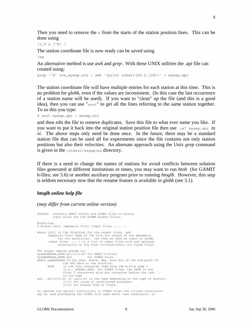
Then you need to remove the X from the starts of the station position lines. This can be done using :1,$ s /^X/ /

The station coordinate file is now ready can be saved using :wq

An alternative method is use awk and grep . With these UNIX utilities the .apr file can created using: grep '^X' svs_myexp.svs | awk '{print substr($0,2,128)}' > myexp.apr

The station coordinate file will have multiple entries for each station at this time. This is no problem for globk, even if the values are inconsistent. (In this case the last occurrence of a station name will be used). If you want to "clean" up the file (and this is a good idea), then you can use "sort" to get all the lines referring to the same station together. To so this you type: % sort myexp.apr > myexp.srt

and then edit the file to remove duplicates. Save this file to what ever name you like. If you want to put it back into the original station position file then use :w! myexp.apr in vi. The above steps only need be done once. In the future, there may be a standard station file that can be used all for experiments since the file contains not only station positions but also their velocities. An alternate approach using the Unix grep command is given in the /stdrel/examples directory. If there is a need to change the names of stations for avoid conflicts between solution files generated at different institutions or times, you may want to run htoh (for GAMIT h-files; see 5.6) or another auxiliary program prior to running htoglb. However, this step is seldom necessary now that the rename feature is available in globk (see 3.1). htoglb online help file (may differ from current online version) HTOGLB: Converts GAMIT hfiles and SINEX files to binary input files for the GLOBK kalman filter. Runstring: % htoglb [dir] [ephmeris file] <input files ..... > where [dir] is the directory for the output files, and [empheris file] Name of the file for output of the ephemeris for the satellites. Can then be used as input to GLOBK. <input files ... > is a list of input files with and optional constraints of the form -C=<constraint> for sinex files. The output naming scheme is: hyymmddhhmm_XXXX.g[l/c][r/x] for GAMIT h-files hyymmddhhmm_XXXX.gls for SINEX files where yymmddhhmm is the year, month, day, hour min of the mid-point of the GPS data in the solution, XXXX is the four character code from the m-file name i (i.e., mXXXXa.ddd). For SINEX files, the XXXX is the first 3 characters plus hte character before the last '.' in the name and .g[l/c][r/x] or .gc[r/x] is the type depending on the type of analyis. [l/c] for loose or constrained analyses; [r/x] for biases free or fixed. To replace the apriori constraints in SINEX files the -C=<new constraint> may be used preceeding the SINEX file name where <new constraint> is


9

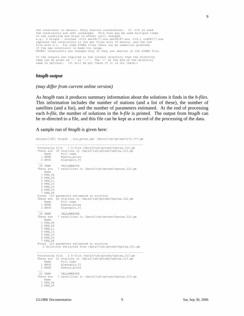
the constraint in meters. (Only station coordinates). If -C=0 is used the constraints are left unchanged. This form may be used multiple times in the runstring and stays in effect until changed. e.g., % htoglb . svsinex -C=10 emr08177.snx emr08187.snx -C=0.1 cod08177.snx replaces the constraints in the emr files with 10 meters, and the cod file with 0.1. For some SINEX files there can be numerical problems if the new constraint is made too large. NOTES: Constraints are changed only if they are smaller in the SINEX file. If the outputs are required in the current directory then the directory name can be given as '.' or './'. The '/' at the end of the directory name is optional. (It will be put there if it is not there.)

htoglb output (may differ from current online version) As htoglb runs it produces summary information about the solutions it finds in the h-files. This information includes the number of stations (and a list of these), the number of satellites (and a list), and the number of parameters estimated. At the end of processing each h-file, the number of solutions in the h-file is printed. The output from htoglb can be re-directed to a file, and this file can be kept as a record of the processing of the data. A sample run of htoglb is given here: meinesz[180] htoglb . svs_gotex.apr /data3/tah/gotexh/h*a.???.gm ---------------------------------------------------------------- Processing file 1 h-file /data3/tah/gotexh/hgotxa.312.gm There are 20 stations in /data3/tah/gotexh/hgotxa.312.gm Name Full name 1 ARGE Buenos_Aires 2 AROG Algonquin_TI ... 20 YKNF YELLOWKNIFE There are 7 satellites in /data3/tah/gotexh/hgotxa.312.gm Name 1 PRN_06 2 PRN_09 3 PRN_11 4 PRN_13 5 PRN_12 6 PRN_03 7 PRN_08 Found 123 parmeters estimated in solution There are 20 stations in /data3/tah/gotexh/hgotxa.312.gm Name Full name 1 ARGE Buenos_Aires 2 AROG Algonquin_TI ... 20 YKNF YELLOWKNIFE There are 7 satellites in /data3/tah/gotexh/hgotxa.312.gm Name 1 PRN_06 2 PRN_09 3 PRN_11 4 PRN_13 5 PRN_12 6 PRN_03 7 PRN_08 Found 123 parmeters estimated in solution 2 Solutions extracted from /data3/tah/gotexh/hgotxa.312.gm ---------------------------------------------------------------- Processing file 2 h-file /data3/tah/gotexh/hgotxa.313.gm There are 21 stations in /data3/tah/gotexh/hgotxa.313.gm Name Full name 1 AROG Algonquin_TI 2 ARGE Buenos_Aires ... 21 YKNF YELLOWKNIFE There are 7 satellites in /data3/tah/gotexh/hgotxa.313.gm Name 1 PRN_06 2 PRN_09


10

3 PRN_11 4 PRN_13 5 PRN_12 6 PRN_03 7 PRN_08 Found 126 parmeters estimated in solution There are 21 stations in /data3/tah/gotexh/hgotxa.313.gm Name Full name 1 AROG Algonquin_TI 2 ARGE Buenos_Aires ... 21 YKNF YELLOWKNIFE There are 7 satellites in /data3/tah/gotexh/hgotxa.313.gm Name 1 PRN_06 2 PRN_09 3 PRN_11 4 PRN_13 5 PRN_12 6 PRN_03 7 PRN_08 Found 126 parmeters estimated in solution 2 Solutions extracted from /data3/tah/gotexh/hgotxa.313.gm

The output continues in this fashion until all of the input files have been processed. The binary h-files produced to this point were h88110706a.glb h88110706a.glc h88110806a.glb h88110806a.glc

The empheris file from htoglb looks like this. The example below is from one of the TREX experiments. (The output has been modified slightly to fit on the page. Any line with a non-blank character in column one is treated as a comment.) * EPHEMERIS INFORMATION FROM /data3/mhm/gpsh/hsv5f7.265 X BLHL -2669008.5659 -4471671.5708 3670491.1942 0.00 0.00 0.00 1987.8 X CENT -2627155.4893 -4596024.6926 3546190.0445 0.00 0.00 0.00 1987.8 X CHUR -236417.0285 -3307611.9855 5430055.7005 0.00 0.00 0.00 1987.8 X FTOR -2697026.6796 -4354393.3301 3788077.5930 0.00 0.00 0.00 1987.8 X MOJA -2356214.5670 -4646734.0343 3668460.4064 0.00 0.00 0.00 1987.8 X OVRO -2410422.3635 -4477802.6741 3838686.7002 0.00 0.00 0.00 1987.8 X PLAT -1240708.0338 -4720454.3507 4094481.6430 0.00 0.00 0.00 1987.8 X PVER -2525452.7058 -4670035.6907 3522886.7474 0.00 0.00 0.00 1987.8 X SCRW -2637874.3720 -4584071.7860 3553275.8946 0.00 0.00 0.00 1987.8 X VNDN -2678071.5492 -4525451.7896 3597427.3893 0.00 0.00 0.00 1987.8 X WSFD 1492233.0781 -4458091.6469 4296045.8718 0.00 0.00 0.00 1987.8 X YKNF -1224064.4364 -2689833.2061 5633432.5576 0.00 0.00 0.00 1987.8 1987 9 22 19 PRN_03 -10842805.007 24243980.669 -3831150.136 -1760766.514 -269167.793 3395719.912 1. 0. 0. 1987 9 22 19 PRN_06 -26388532.444 -36870.803 -2515352.661 316091.153 -1697082.150 -3476692.138 1. 0. 0. 1987 9 22 19 PRN_08 -2360574.007 -16647057.910 20711471.760 2401791.966 -2486239.881 -1710717.332 1. 0. 0. 1987 9 22 19 PRN_09 -21900797.485 7386881.149 12962283.044 -2220086.711 -1310718.902 -2903249.941 1. 0. 0. 1987 9 22 19 PRN_11 -12163772.008 -2711902.697 23667026.292 1647771.210 -3451673.884 409341.317 1. 0. 0. 1987 9 22 19 PRN_12 -7079308.878 11797055.590 22974615.291 -3705252.412 -310016.283 -967240.583 1. 0. 0. 1987 9 22 19 PRN_13 -16347959.701 15918699.005 13536254.127 -235747.117 -2638855.996 2832298.920 1. 0. 0. * EPHEMERIS INFORMATION FROM /data3/mhm/gpsh/hsv5f7.265 X BLHL -2669008.5659 -4471671.5708 3670491.1942 0.00 0.00 0.00 1987.8 X CENT -2627155.4893 -4596024.6926 3546190.0445 0.00 0.00 0.00 1987.8 X CHUR -236417.0285 -3307611.9855 5430055.7005 0.00 0.00 0.00 1987.8 X FTOR -2697026.6796 -4354393.3301 3788077.5930 0.00 0.00 0.00 1987.8 X MOJA -2356214.5670 -4646734.0343 3668460.4064 0.00 0.00 0.00 1987.8 X OVRO -2410422.3635 -4477802.6741 3838686.7002 0.00 0.00 0.00 1987.8 X PLAT -1240708.0338 -4720454.3507 4094481.6430 0.00 0.00 0.00 1987.8 X PVER -2525452.7058 -4670035.6907 3522886.7474 0.00 0.00 0.00 1987.8 X SCRW -2637874.3720 -4584071.7860 3553275.8946 0.00 0.00 0.00 1987.8 X VNDN -2678071.5492 -4525451.7896 3597427.3893 0.00 0.00 0.00 1987.8 X WSFD 1492233.0781 -4458091.6469 4296045.8718 0.00 0.00 0.00 1987.8 X YKNF -1224064.4364 -2689833.2061 5633432.5576 0.00 0.00 0.00 1987.8 1987 9 22 19 PRN_03 -10842805.007 24243980.669 -3831150.136 -1760766.514 -269167.793 3395719.912 1. 0. 0. 1987 9 22 19 PRN_06 -26388532.444 -36870.803 -2515352.661 316091.153 -1697082.150 -3476692.138 1. 0. 0. 1987 9 22 19 PRN_08 -2360574.007 -16647057.910 20711471.760 2401791.966 -2486239.881 -1710717.332 1. 0. 0. 1987 9 22 19 PRN_09 -21900797.485 7386881.149 12962283.044 -2220086.711 -1310718.902 -2903249.941 1. 0. 0. 1987 9 22 19 PRN_11 -12163772.008 -2711902.697 23667026.292 1647771.210 -3451673.884 409341.317 1. 0. 0. 1987 9 22 19 PRN_12 -7079308.878 11797055.590 22974615.291 -3705252.412 -310016.283 -967240.583 1. 0. 0. 1987 9 22 19 PRN_13 -16347959.701 15918699.005 13536254.127 -235747.117 -2638855.996 2832298.920 1. 0. 0.

htoglb error messages


11

Htoglb generates only a few error messages. The most common of these is that it can't find a h file (if the name is explicitly given for example), or that a selected file is not a h file (in this case the first line in the file which did not match the expected pattern is printed). This error may be generated if the version of GAMIT producing the h file is inconsistent with the version of htoglb being used. File errors generated by htoglb (and most of the other programs in the suite) are of the form: <Type> error <nnn> occurred <action>ing <file> in <module name>

and then possibly, depending on the severity of the error, Program terminating in <module name> stop in report_error

where <Type> is the type of error. This will usually be: IOSTAT for standard fortran input/output errors, FmpOpen/Read/Write for binary file manipulation errors, and in some cases VREAD/VWRITE for large binary file manipulations. <nnn> is the error number. For IOSTAT errors, these can be found in the fortran

manuals. Some important ones to remember are -1 is EOF 118 is file not found.

For the other classes of errors, -1 means EOF, and -6 means file not found. In general (except for the -6 error) the Fmpxxxx class of errors are the negative of the fortran IOSTAT errors. A -1 error when a string is being decoded means that there were not enough items in the string to satisfy the read. (Usually because something has been forgotten.) The other class of error is 112 meaning illegal character in format which usually means that a non-numerical value was encountered when one was expected.

<action> is the action being carried out when the error occurred. These generally fall into the classes of opening, reading, writing, decoding with the last of these usually used only for string manipulation.

<file> is the name of the file being worked on at the time, or for decoding errors, the string (or part of it) which was being manipulated.

<module name> is the name of the subroutine where the error occurred. This is sometimes as general utility routine (such as read_line or multiread) and it could be difficult to determine exactly where the error occurred. In these cases either the string or the file name is useful for isolating the error.

2.2 apr_file Although the file of apriori station coordinates can be extracted from the htoglb output, most frequently we use a standard file of ITRF positions and velocities (available in the


12

updates/sites directory in the software distribution area). After an initial solution, the coordinates of new stations can be added to this file (or used as a supplementary file—see the apr_file command in Section 3.1) by extracting them from the print (.prt or .org) output of globk or glorg. Specifically the print file includes a listing of the estimated cartesian coordinates and velocities at the midpoint time of the solution in apr_file format but with the character string 'Unc.' in the first four columns; hence the command grep 'Unc.' [apr file name] > temp.apr will write these coordinates to the file temp.apr; to complete the task, you need to remove 'Unc.' from the first columns of the output. A new feature with version 5.03 is to allow non-secular terms to be added to the apriori coordinates of the stations. These terms are added using a additional lines in the apr_file, detected by EXTENDED being the first token on the line. The additional terms can be periodic, exponential, or logarithmic or changes in the postion and rate. The format of the new lines is as follows: EXTENDED <Site Name> <Type> <YY MM DD HR MN> <Parameter> <Coefficients for NEU> where EXTENDED should be preceeded by at least one blank. The line is not case sensitive. The following <Types> are allowed EXP Exponential variations: The exponential starts at the time given by <YY MM DD HR MN> and the <Parameter> is the decay time, in days, for the exponential (ie. exp[-dtime/Parameter] where dtime is time after the start time. The coefficients are the amplitudes for North, East and Up. Units meters. Example: EXTENDED JPLM_GPS EXP 1992 6 28 0 0 30.0 0.010 0.005 0.00 results in 30 day exponential with amplitude of 10 mm North, 5 mm East and zero for the height LOG Logarithm variations: The logarithmic function is applied after date <YY MM DD HR MN> and the <Parameter> is time normalization value in days (ie., log(dtime/Paramter) where dtime is time from the start time. The coefficients are the amplitudes for North, East and Up. Units meters. Note: No data should be included that is within the normalization parameter of the start time (i.e., log(0) = -infinity). Example EXTENDED JPLM_GPS LOG 1992 6 28 0 0 300.0 0.010 0.005 0.00 Results in 300 day logarithmic with amplitude of 10 mm North, 5 mm East and zero for the height PERIODIC periodic variations: Applied to all dates. The <YY MM DD HR MN> is the zero phase time of the periodic signals and the <Parameter> is the period in days (i.e., cos(2*pi*dtime/Parameter) where dtime is time from <YY MM DD HR MN>. The coefficients are paired as the cosine and sine coefficients for North, East and Up. Units meters. Example EXTENDED JPLM_GPS Periodic 2000 1 1 0 0 365.25 0.0 0.0 0.0 0.0 0.001 0.009 results in annual signal in height with cosine amplitude of 1 mm and Sine amplitude of 9 mm. OFFSET Episodic change in position and velocity. Applied after <YY MM DD HR MN> <Parameter> in this case is not used (value of 0.0 should be given). The coefficients are paired as offset and rate changes applied after the start date (i.e., offset + dtime*rate where dtime is time after start time. Units: offset meters, rate meters/year. Example: EXTENDED JPLM_GPS Offset 1992 6 28 0 0 0.0 0.003 0.001 0.004 0.004 0.000 0.000 results in north position and velocity change of 3 mm and 1 mm/yr, East position and velocity change fo 4 mm and 4 mm/yr. No change in height.


13

Each of the terms given should be unique. If duplicates (in terms of epoch, type and parameter) are given, the lastest one read will be used. This extended model is meant for use with time series analysis. The non-secular terms are saved in any out binary h-file. The position estimates and adjustment output by globk and glorg include these terms evaluated at the epoch of the output solution. Finally, notes that the EXTENDED feature of the apr_file differs in the way it handles position changes from hfupd (Section 5.6) and the eq_file rename feature (Section 3.1). The eq_file rename changes the "observed" station position in the input hfile whereas the EXTENDED feature in the apr_file changes the "modeled" position. Thus, the signs are opposite to acheive the same effect. To correct erroneous heights in h-files, hfupd is now the preferred means. the EXTENDED offset feature in the apr_file should only be used with glred for repeatability runs to account for coseismic offsets and rate changes, whereas the eq_file feature and hfupd are used in globk runs when velocities are to be estimated.


14

3. RUNNING GLRED, GLOBK, AND GLORG To run glred or globk you will need a file with a list of quasi-observation (binary h-) files to process, a file of a priori coordinates and velocities for the stations, a table of Earth orientation parameter values for the times of your data, and globk and glorg command files. The easiest method of generating the input global file list is to use the ls command. Conventionally the list files are given with a .gdl extent (global directory list) but the name is arbitrary. For example, to generate a gdl file for the biases-free h-files you have created (with htoglb) for the 1996 Eastern Mediterranean survey, you might use % ls ../glbf/h*.glr > emed96_free.gdl

To obtain an alternate list for the biases-fixed h-files, you might use % ls ../glbf/h*.glx > emed96_fxd.gdl

The .gdl file may optionally contain additional parameters following each h-file name to indicate reweighting and coupling; e.g. h9609061159_igs1.glr 1.0 + h9609061159_igs2.glr 1.0 + h9609061159_emed96.glx 4.0

where the numbers indicate the relative weighting of the estimates and covariance matrix in the solution (e.g., the third h-file is to be downweighted by 4.0 [a factor of 2 in uncertainty]); and the + specified for the first two files links all three together (applicable only for glred—see Testing coordinate repeatabilities in Section 3.4). There is an optional additional value that can be included on each line to rescale the diagonals terms of the covariance matrix. It is given in parts per million to be added to 1.0 and is useful primarily for stabilizing SINEX files which have had their constraints removed. An example of the use of this parameter is h980126_stan.glx 4. 2 +

which would scale the covariance matrix by 4.0 and the diagonal elements additionally by (1.0 + 2*1.d-6). The command file is either created with an editor or copied from a previous example (such as those given in Section 3.4). The command file controls the actions of globk through the use of commands of three types: (1) Names of files: the scratch files used by the program, and the files containing a priori

station positions, satellite ephemeris information, and earthquake/rename commands.

(2) Output options which can be used to tailor the output for a desired run. (This becomes a means for eliminating output that will not be needed.)

(3) Specification of the uncertainties and the stochastic nature of the parameters in the solution. These commands also determine which parameters are estimated, and how the information in h-files is treated.

For commands of types (1) and (2), if a file or option is not mentioned, it will not be used. Thus, for example, to invoke glorg from within globk, you must include org_cmd


15

with the name of the glorg command file; and to get a globk back solution, you must include bak_file with the name of the back solution print file. Commands of type (3) are more complicated since they depend on how the parameter was treated in the analysis that produced the h-file and in some cases on combination of parameters estimated. For parameters estimated in the previous analysis (i.e., present on the h-file) entering a non-zero value in the apr_ command assigns an a priori standard deviation of that value to the parameter. If the parameter has been constrained in the previous solution, that constraint is not removed or altered, but rather the new value is added to it. Thus, we recommend that you do not apply constraints any earlier than you need to—only at the very last stage (glorg) for station coordinates and at the time of daily combination for orbital and Earth orientation parameters. Markov command (mar_) add process noise with each new h-file, so that they have the effect of loosening the a priori (apr_) value over time. Station coordinate and orbital parameters must be present on the input h-file in order to be used in the solution or have constraints applied. For station velocities and Earth orientation parameters (EOPs), however, globk can generate partial derivatives and add these to the solution even if they were not on the h-file. If a value of zero is entered for a parameter or if the parameter is not mentioned in the command file (no apr_ command), the result depends on whether it was on the input h-file and whether it is coupled to other parameters that are estimated. In most cases (station parameters and velocities, orbital parameters) entering zero or omitting an entry means to ignore the parameter and take no action. This means that if a parameter is included in an input h-file and you don't mention it in the command file, it will implicitly retain the constraints that it had originally while not being listed explicitly in the solution. For example, if the h-file from the primary data analysis was created (e.g., by GAMIT) with loose constraints on orbital parameters and you omit the apr_svs command, the orbits remain implicitly loose in the globk solution; if the orbit was constrained in an earlier solution, those constraints implicitly remain (through the station coordinates and EOPs) even though the orbital parameters no longer appear in the solution. A special case arises when estimating EOPs since they are directly coupled to station coordinates. In this case, entering zero for any station coordinate will cause it to be fixed and used to determine the EOPs. In some cases, we want to explicitly fix a parameter without relying on the implicit rules used in globk. In these cases, the letter F can be used for the apriori uncertainty of a parameter. (Giving zero for the a priori sigma will not work because zero would generate the same action (or lack there of) as not saying anything about the parameter.) F for an uncertainty will be interpreted as zero uncertainty in the apriori value of the parameter (i.e., fixed) but the parameter will be given parameter space and included in the output of the program. (This latter feature is useful for keeping a record of the exact values of the parameter used in the solution.) In summary, the basic rules of globk’s interpreter are (consult the example command file below for commands): (1) The apriori values of parameters (station positions and velocities, and satellite orbit information) are taken from the files given by the apr_file and the svs_file. If some


16

quantity does not appear in these files, then the apriori value will be the apriori value from solve (post 3.2 versions of htoglb) or the estimate of the parameter from its last occurrence in the input global files. (If the parameter was originally fixed in solve, then this value will used.) (2) If any parameter that does not explicitly depend on other parameters is given zero uncertainty (either explicitly or by neglect), it will not be constrained at all, and it will not appear in the output of the solution. (Use of the all option for station and satellite names allows easy assignment of uncertainties to all parameters.) (3) If any parameter that does explicitly depend on other parameters that are being estimated, is given zero uncertainty (either explicitly or by neglect), it will be fixed to its apriori value (independent of where this value comes from, see 1). Even though it is fixed, its value will not appear in the output. If you want to explicitly control globk use the F option for the uncertainty of a parameter you wish to fix. If the three rules above are kept in mind, then it should not be difficult to get globk to do the solution you want. Since globk solutions usually take only a few minutes to run for a typical GPS campaign, and less than half an hour for a complete sequence of experiments, it is recommended that you play a little with the options and the implicit rules just to be sure that you understand them. Orbits are treated somewhat differently from other parameters in globk. The integration epoch of the orbit (i.e., the epoch to which the orbital elements refer) is passed from arc through the h-files to globk and globk keeps track of this quantity. While the IC epoch remains the same, the stochastic parameters associated with the orbital arcs are used. However, when the IC epoch changes, the uncertainties that were given for the apriori values of the orbital elements are reimposed on the estimates, thus effectively breaking the multiday orbital arc. Whenever, the IC epoch changes, globk prints a message to std out saying that it is updating the IC epoch. These messages should be checked when data is first processed to ensure that the correct multiday orbital arcs are being used. (For example, an incorrect reference to a t-file could cause a break in the middle of a multiday orbit arc.) The parameters representing satellite antenna offsets, though associated with the orbital parameters, are not treated on an arc-by-basis, but rather globally, so that that a single set of parameters is used for each satellite for a solution. To run globk you type: % GLOBK <std out> <print file> <log file> <experlist> <command file> <option>

where <std out> is a numerical value (if 6 is typed then output will be sent to current window,

any other numerical value will send output to a file fort.nn) <print file> is a numerical value or the name for the output print file with the solution

in it. If the print file already exists, then the solution will be appended to it unless ERAS is specified for prt_opt. For output to your current window, 6 may be used.

<log file> is a numerical value for the log file that contains the running time for the program and the prefit c2 per degree of freedom value for each input covariance


17

matrix file. If the log file already exists, then the new log will be appended to it. For output to your current window, 6 may be used.

<exper list> is a list of binary h-files to process. Any file name may be used but convention is to end it with .gdl.

<command file> is a list of commands controlling the solution. <option> designates a string that may appear in the first line of the command-file

indicating that this is the particular version of the command file to be executated. The string should begin in column 1 so that it is interpreted as a comment in reading the commands themselves.

The next two sections describe in detail the commands of the globk/glred and glorg command files. Following these, in Section 3.3, we describe in both theoretical and practical terms the various approaches you might take to defining a reference frame for GPS data analysis. Section 3.4 gives examples for analyzing daily solutions to obtain a time series for error analysis and for combining multi-year solutions to obtain a time series or velocities. The last two sections of this chapter give examples of glred/globk and glorg outputs and error messages. With GAMIT/GLOBK release 10.0 there is a new script sh_glred that allows you to combine efficiently large numbers of H-files from a global and/or regional analysis and plot the time series. Since the control files for this script are the same as for sh_gamit, it is described in the GAMIT manual. 3.1 globk command file ********************************************* * Annotated example of a GLOBK command file * * (used for the analysis of GPS Data). * ********************************************* * * General rules: * ------------------ * (1) All commands start with a blank in column one. All other lines, * including blank lines are considered comments and are ignored. * This also applies to apriori station and satellite position files. * Comments may also add at the end of any command line by using the * ! or # character as a delimiter. * (2) Only the minimum redundant set of characters for commands, site * names or satellite names are needed. For clarity, it is recommended * that the full command or name be given. This also avoids problems * with future releases of the software where the minimum redundant * sequences may change when new commands are introduced * (3) Satellite names are of the form PRN_nn where nn is the PRN number * of the satellite. These names are generated by htoglb. (Most of * the time individual satellite names are not needed.) * (4) In general the order in which commands are given has no effect ex- * cept that the second issuance of a command overwrites the effects * of the first (for the specific case given, see below for example * of the application of this feature with station coordinates). * However, There are three commands that will have no effect * unless they are issued before all others. They are the COM_FILE, * SRT_FILE, SRT_DIR, MAKE_SVS, and EQ_FILE commands, as described * below.


18

* (5) Blank lines are ignored, and may be used to structure the command * file. * (6) All file names may be absolute or relative (i.e,../tables/glb.apr) * and are limited in length to 128 characters. * (7) Case is not important. All strings (except file names and * descriptors are converted to upper case.) This does mean however * that station names passed to globk must be uppercase (this is * currently the case). * (8) Groups of commands that are shared between different globk (or * glorg) input files can be included via the SOURCE command, which * can be issued one or more times after the required initial files * describe in (4). For example, source site_constraints could be * used to insert a set of apr_site commands (see below) contained * in the file 'site_constraints'. * Start the command file * ====================== * * The following five commands, if present, must be issued before all * others or they will have no effect: * * Set the names for the "scratch files".

com_file glbcom.bin ! Contains the globk common blocks srt_file glbsrt.bin ! Contains direct access time-ordered list * ! of global files * These files do not need to exist before hand, they are simply used to * save intermediate results. The com_file is used to store information * that is needed to rerun the output program glout and the reference- * frame-fixing program glorg If you are not calling glorg from within * glred in performing daily solutions, you can save time by omitting * the com_file command and hence not writing out the solution. (Program * globk currently writes the com_file automatically whether you specify * a name or not, but this will be changed in the future.) Note that the * com file is not backward compatible between versions of the software. * If you want the data processed in reverse time order, then uncomment * the line below. If this is done the station coordinates, Earth * rotation parameters, and satellite orbit parameter will refer to the * first epoch of data and not the last as it does in the default case # srt_dir -1 * * The preferred method for generating the a priori values of satellite * parameters now is to read them from the input binary h-files and write * them to a file specified at the top of the command file: make_svs svs.apr [ Z ] * When h-files from the same day are combined, the elements from * the first hfile read will used. If the svs file already exists, it * will be overwritten. If the make_svs command is missing, globk will * look for the svs_file command which was formerly used to specify a * list of apriori* satellite parameters written by htoglb or unify_svs: * apr_svs <filename> * If the optional Z is specified after the file name then the radiation * parameters are set such that the direct radiation is 1.0 and all * the other radiation pressure parameters are zero. This option is * useful for stabilizing orbital solutions but can have adverse * consequences if you tightly constrain a parameter that has been * correctly adjusted to a non-zero value. When the rad_rese command is * used, it is recommended that the Z-option be invoked. The default is * not to invoke it.


19

* If you have an earthquake file, necessary for earthquake parameters * and station renames, it must be entered here: eq_file landers.eq * Additional commands in any order: * ================================= * Now start the commands which do not depend on order. (When the first * of these commands is issued, the program will first read all of the * input global files and build up the list of stations and satellites to * be used in the analysis. * One more scratch file is needed. This file contains the covariance * matrix for the solution, and if a back solution is to be run then * contains the covariance of each global file in the solution. (In * this latter case the file can get very large. Generally it is less * than 1 Mbyte per global file, but for VLBI with over 1000 experiments * is over a Gbyte.) sol_file glbsol.bin * Filtering input data * ==================== * You can have glred or globk automatically exclude from its solution * h-files that contain corrupted data or a station for which you have * no reasonable a priori coordinates using the command MAX_CHII <max chi**2 Increment> <max prefit difference> <max rotation> where the three arguments give tolerances on the chi-square increment, change in a priori parameter values, and allowable pre-solution rotations of a network before combining a new h-file. <max chi**2 Increment> gives the maximum allowable increment in the chi**2 when a new h-file is combined in the solution. In this version of globk these data will not be added to the solution and the solution will continue to run. The same procedure will happen with negative chi**2 increments (which result from numerical insatabilities and can be solved often by tightening the apriori constraints and reducing the magnitudes of process noise on the stochastic parameters. More detail diagonistic information is now output to the log file if a negative chi**2 increment occurrs. The default value of max_chii is 100.0. <max prefit difference> is maximum difference in the prefit residual for station coordinates. This value also sets the limits for other parameters in globk but with the input value internally scaled to provide comparably reasonable tolerances for the other parameters. For EOP, the prefit tolerance is 10 times the surface rotation implied by the station coordinates, and for orbital initial position and velocity, 1000 times the station tolerance. If the prefit difference exceeds this limit, then the estimate for this parameter is not included (row and column removed from the covariance matrix), or in the case of a station coordinate, all three coordinates are excluded. The default is 10,000, corrsponding to 10 km for a station position. When the aprioris are well known, this value can be set small (e.g., 0.1 for global networks with good orbits, corresponding to 10 cm for station position, 32 mas for EOP, and 100 in orbital initial position). <max rotation> sets the tolerance for a rotation of the prefit station coordinates before they are compared with the current solution. This check complements the new feature of globk in which an orientation


20

difference between the stations of the input h-file and the current is computed. If this value exceeds <max rotation>, then the rotation is removed from the station coordinates and added to the EOP parameter estimates and a message is written to the screen. The purpose of this feature is to avoid having to set the Markov values of the EOP parameters inordinately large to handle a few h-files for which the EOPs of the phase processing had large errors. For global networks, the rotation can be determined well from data, so setting a small <max rotation> value (e.g. 20 mas) is useful to maintain small Markov values. For regional networks, the rotation is poorly determined, so the tolerance should be kept large to avoid erroneous rotations that can cause numerical problems. The default is 10,000 mas. * Station coordinate file * ======================= * File containing a list of a priori station coordinates and velocities * to be used in the solution file (input). The file is free format, but * must contain: * * Site_name X Y Z Xdot Ydot Zdot Epoch * * where XYZ are Cartesian geocentric coordinates in meters, * Xdot Ydot Zdot are rates of change of these coordinates (m/yr) * and Epoch is year and fractional year (i.e., 1990.27) to which the * coordinates refer. apr_file grece.apr * Reissuing the apr_file will result in additional files being read, * with the coordinates for a station taken from the last file in which * that station appeared. * A priori Earth-rotation table * ============================== * Command to allow the polar motion/UT1 series used in the analysis to * updated. Form: * * in_pmu <file name> * * where <file name> is a file containing the new series. The pole * position and UT1 values must be uniformly spaced, and the UT1 should * NOT be regularized. The format of the file (matchs the IRIS format) * is * yyyy mm dd hh min X-pole +- Y-Pole +- UT1-AT +- * (asec) (asec) (tsec) 1980 1 1 0 0 0.1290 0.001 0.2510 0.001 -18.3556 0.0001 1980 1 6 0 0 0.1250 0.001 0.2420 0.001 -18.3682 0.0001 etc * * NOTE: The sigmas on the values are not used in globk. * NOTE: This command only works with post-9.10 releases of solve. * Performing a back solution * =========================== * * The bak_file command invokes a Kalman back solution, allowing you to * see the estimates for stochastic parameters, e.g., in testing * repeatability of coordinates or baselines. The name of the back- * solution file is arbitrary, but has .bak as an extent. If this file * exists, it will be appended by subsequent runs, so you should usally * delete previous versions before running. Running a back * solution will generally treble the run time for the solution, and is


21

* not needed unless you want to extract the values obtained for the * markov elements (e.g., orbits, polar motion, UT1-AT). It is not * necessary to run the back solution if you are only interested in * station positions and velocities for example. If the back solution * is to be run, then the DESCRIPT command should also be given so that * you don't get nulls as the first line of output file. When a back * solution is run, you have the option of generating post fit parameter * residuals using the comp_res command. For the very loose GPS * solutions used at the moment this is not a particularly useful feature * It also doubles the length of time needed to do the back solution. * Currently it is recommended that this command not be used. (The * command is commented out below) bak_file grece_fxd.bak descript Test run of network with orbits and station DDDD fixed. # comp_res yes * The form bak_file @.bak may also be used for the file name in which * case the @ is replaced by corresponding characters from the experiment * list file. i.e., for the case above, if grece_fxd.gdl was the * experiment list, the bak file name would be grece_fxd.bak. * * Print commands * ============== * * The output from globk is normally produced twice, once to your screen * and once to your print (prt) file specified in the runstring. If a * back solution has been commanded by specifying a bak_file, then a * second file output is produced. The quantities to be written to the * two files and the screen are specified separately with the prt_opt, * bak_opt, and crt_opt commands, respectively. The specification is * made with either a 4-character keyword or a binary-coded (bit mapped) * integer value. The keywords, corresponding bits, and their meanings are * as follows: * * CODE BIT Decimal Meaning * ---- --- ------- -------- * CORR 0 1 Output correlation matrix * BLEN 1 2 Output baseline lengths and components * BRAT 2 4 Output baseline lengths and components rates * of change. * CMDS 3 8 Write a summary of the globk command file to the * globk and glorg output files. * VSUM 4 16 Write the short version of the velocity field * information (one line per station) * 5-9 32-512 NO LONGER USED (see POS_ORG and RATE_ORG below. * RAFX 10 1024 Fix the Right ascension origin of the system. * MOUT 11 2048 Only output baselines if both stations are Markov. * (Used to limit output in large back solutions) * COVA 12 4096 Output full precision covariance matrix. * PSUM 13 8192 Output position adjustments in summary form * GDLF 14 16384 Output the contents of the GDL files used * DBUG 15 Output matrix details when there are negative * variances and negative chi**2 increments * ERAS 16 Erase the output file before writing solution * NOPR 17 Do not output the file (either crt, prt or org * depending on opt set). * * For example,to write to the print file baseline lengths, baseline rates, * and a summary velocity field, set prt_opt blen brat vsum * or, equivalently, prt_opt = 22


22

* A value of -1 will print everything. This is not recommended since * there are coordinate rank deficiency handling routines which are * invoked when all bits are set. If no command is given, then only the * parameter estimates, adjustments, and sigmas will be output. * * In the back solution, only printing of baseline length and components * is implemented. * bak_opt blen * * For back solutions there is an additional print command that allows * the user to specify which stations should always be printed in the * bak_file. It has the form * * bak_prts clear all <list of stations> * * where the CLEAR is optional and should normally not be used since * it will override the internal rules for outputting a station. ALL * will select all stations. The following rules apply for outputting: * * --Site positions--: * All and only sites that are Markov (i.e. mar_neu or mar_site command * * used) or are affected by an earthquake (see eq_file command) will be * output unless CLEAR is used in the bak_prts commands, in which case * only those sites listed in the bak_prts command will be printed * independently of whether they are Markov or affected by an earthquake. * In all cases, only sites that were observed on the day being output * will be printed. * --Baselines and baseline components--: * In general, for a baseline to be printed, both sites in the baseline * need to pass the criteria to be output. For baselines to be printed * bak_opt bit 1 (decimal value 2) must be set. If only bak_opts 2 is * set all baselines between sites observed on the day will be printed. * (This can become a long list). Restrictions can be placed on the * baselines printed using bak_opt 2050, where bits 2 and 11 have been * set to restrict the baselines to only those affected by an earthquake, * (including pre and post-seismic intervals extended by 2 days) or are * Markov. Use of bak_prts allows additional sites to be printed that do * not pass the earthquake or Markov rules. bak_prts eeee ffff ! Always output these two sites * * Creating a combined h-file * ========================== * * The OUT_GLB command allows a binary h-file to be generated with globk. * Thisfeature is typically used to combine all the data collected in a * single experiment into a single h-file for later processing * out_glb [email protected] * * where @ takes in the chanracters from the experiment list file, .e.g. * if the experiment list was exp_June92.gdl then the output global file * would be com_June92.GLX. If you forget to set out_glb in your globk * run, you can create an output binary h-file from the globk com_file * the new program glsave, described in section III.e. * * Selecting stations * ================== * * A station may be excluded from the analysis by name, geographical * region, or the number of times it appears in the input h-files. The * default is to include all stations that appear in the h-files. To * exclude by name, use the USE_SITE command, either starting with CLEAR


23

* to exclude all, and then adding the names of those you wish to include, * or starting with ALL (default) and subtracting those you wish to * exclude: * * use_site clear * use_site sit4 sit5 sit6 ...etc. * * or * * use_site -sit1 -sit2 -sit3 * * This command may include wildcards (@) to force use of renamed statins * (e.g. use_site gold@ would Include gold_gps, gold_1ps, gold_1la, etc.) * * To select by region, use the USE_POS command to define a box * within which you want to include or exclude stations: * * use_pos < +/- > <Lat LL> <Long LL> <Lat UR> <Long UR> * * where + indicates inclusion and - exclusion of stations within * the box defined by the latitude and longitude (postive east) of * its lower-left (LL), and upper-right (UR) corners. Thus the command * * use_pos - 30.0 -125 35.0 -115. * * specifies exclusion of stations between 30 and 35 degrees north * and 115 and 125 degrees west (i.e., southern California). This * command is used in conjunction with use_site. If use_site clear * is initially specified, the use_pos + can add stations within a * defined region; conversely, is use_site all is initially specified, * use_pos - can remove stations with a region. The use_site command * can be issued after use_pos to add or remove specific stations by * name. * * To select stations on the basis of the number of times they have * been observed, use the USE_NUM command followed by an integer * specifying the minimum number of times a station must appear in the * h-files in order to be included in the analysis. The command is * applied after all 'use' options have been processed, so that it * affects only stations that are otherwise included. * * Selecting and constraining parameters to be estimated * ===================================================== * * For each type of parameter in the solution there are commands * to specify the a priori sigmas. Since a Kalman filter requires * some level of a priori constraint, if these commands are omitted * for a particular group of parameters, these parameters will be * ignored in the the input binary h-files. This is equivalent to * allowing the parameter to freely vary between sessions of the data. * * You can also allow parameters to vary stochastically between * observations (i.e., h-files) by specifying Markov process noise to * be added. Specifically, the variations are modeled as random walks * with a specified power spectral density (PSD) of the white noise * noise process driving the random walk. Since the variance of the * difference between two values in a random walk is given by PSD*dT * where dT is the time difference in the units of the PSD time argument, * you can easily compute how a given value will affect the solution. * For example, a PSD value of 36500 m**2/yr for station coordinates * will constrain the station position to +-10 meters (one sigma) between * sessions separated by a day. Specifying stochastic variation of * of parameters is an effective way of absorbing errors due to * unmodeled behavior, such as the effects of non-gravitational forces * on satellites, errors in a priori Earth-rotation information, post-


24

* seismic motion of stations. It is also a useful way of handling * apparent changes in station position due to changes in instrumentation * or blunders in measuring antenna heights. Finally, allowing * stochastic variation of station coordinates and running a Kalman back * solution may be used to test the repeatability of the values in a set * of data, though for most data sets this can be done more efficiently * by treating each day (h-file) independently and ruuning glred instead * of globk (see section III.d below). * Station coordinates and velocities * ---------------------------------- * * Apriori constraints on site positions and velocities are expressed as * one-standard-deviation uncertainties. If an apr_file command has been * used then these refer to the values in that file, otherwise they are * are the estimated values found in the global files. The constraints * may be specified either in cartesian coordinates x, y, z, using the * command apr_site, or north, east, up, using apr_neu. The units are * meters for position and meters/year for velocities. In the case * below, there are no velocity sigmas given, so velocities will not be * estimated. An efficient way to enter the constraints is to first * set the default using "all", and then follow with overriding values * for specific stations. apr_neu all 100 100 100 0 0 0 apr_neu ssss .01 .01 .05 0 0 0 * Warning: If both apr_site and apr_neu are entered, the a priori * sigmas will be combined (added quadratically). This is true even * if "all" if used for one of the commands, so be careful. * * To absolutely fix a station (as opposed to heavily constraining * it, you can use "F" for the apriori sigma. This will set aside * parameter space for the site, but the site position will be given an * apriori position uncertainty of zero. Fixing with local coordinates * is not recommended since globk works internally it in Cartesian * coordinates, and the zero value can lead to (small) negative variances * at the end of the solution. apr_site dddd F F F 0 0 0 * To add (random) noise to the coordinates of individual stations, you * may use the command * sig_new <station> <hf code> <NEU sigmas> <start date> <end date> * where <station> is the leading 4- or or full 8-character site code, * <hfcode> is string of H-file names to be searched, <NEU sigmas> are * the noise sigmas in meters, and the last two entries give the calender * dates of the range, in YYYY MM DD HH MM. For example, to add 20 mm * of vertical noise to all Auckland (AUCK_) stations between 1 February * and 1 March, 1999, use sig_neu auck .0 .0 .02 1999 2 1 0 0 1999 3 1 0 0 * Both the H-file name and time span entries are optional. There is * a 1-minute (inclusive) tolerance on the time entires. You can apply

* noise to a group of renamed stations using @[string];* e.g., @_BAD * would match all stations renamed to end in _BAD. * All entries which apply to a station are used (in a variance sum)> * To add Markov (time-dependent) noise to the coordinates of stations, * the form is similar to the apr_ commands but with units of m**2./yr. * We turn off the Markov process at one station so that the system will * have a fixed origin: mar_site all 36500 36500 36500 0 0 0


25

mar_site dddd 0 0 0 0 0 0 mar_neu eeee 0 0 36500 0 0 0 ! Markov height only at * ! this station. * * Be careful not to trying estimating velocities for stations when * the coordinates have non-neglibile Markov process noise. Although we * do not usually input Markov constraints for velocities, this can be * done, with the result that the process is assumed to be a random walk * in velocity (as for all parameters) and therefore an integrated random * walk in position (see the discussion in Herring et al.[1990]). Wildcards * (@) can be used with these commands (e.g. mar_neu gold@, @_gla). * Satellite orbital parameters * ----------------------------- * * Satellite parmeters are defined in the same way as in GAMIT, but * the units for the initial conditions are different--here meters * and millimeters/second. The change in units (from GAMIT) is needed * because Kalman filters suffer fewer rounding error problems when all * the units generate similar size numerical values. apr_svs all 200 200 200 20 20 20 apr_rad all 1. 1. .02 .02 .02 .02 .02 .02 .02 .02 .02 .02 .02 .02 apr_svan all .01 .01 .01 * The second token in these commands can be ‘all’ to refer to all * satellites, or the name of an individual satellite, e.g., prn_01. * The constraints for non-gravitational parameters (dimensionless) refer * to the 14 parameters now allowed by GAMIT and must be in the following * order: DRAD YRAD ZRAD BRAD XRAD DCOS DSIN YCOS YSIN BCOS BSIN. * X1SN, X3SN, Z1SN (see gamit/arc/ertorb.f for definitions). Normally, * you would have used a consistent 3-, 6-, or 9-parameters model, so * that only subsets of these would be meaningful. For example, for the * Berne (1994) model (DRAD YRAD BRAD DCOS DSIN YCOS YSIN BCOS BSIN), apr_rad all 1. 1. 0 .02 0 .02 .02 .02 .02 .02 .02 * would set direct and y-bias sigmas at 100%, and the b-axis and once- * per-rev sigmas at 2%. The values for the unused z-axis and x-axis * parameters are set here to zero but would be ignored by globk * since they do not appear in the binary h-files. If differeent * sets of parameters are used in different solutions, you should set * realistic sigmas for all 14 parameters. The non-gravitational * parameter sigmas can also be added to the apr_svs command line * (after the 6 for position and velocity of the satellite). * The third set of satellite parameters are for SV antenna offsets and * have units of meters. * A priori values constraints for the Initial conditions, radiation * pressure, and SV antenna offset parameters can be entered on a single * line as apr_svs, an option that is more feasible with a new feature * that allows a short cut: apr_svs prn_09 10 10 10 1 1 1 1 0.01R 5A * where the first seven parameters (initial conditions and direct * radiation pressure are specified explicitly, the “R” appended to the * next entry indicates that all other radiation pressure parameters are * to have this constraint (1%), and the “A” appended to the last entry * indicates that all SV antenna offsets are to have this constraint (5m) * * If no apr_svs command is given, the effect is the same as specifying * zeroes for the a priori constraints; i.e., whatever constraints were * present in the input h-file will be used and the orbital parameters * will be suppressed in the output. This approach will produce a


26

* quicker solution than weakly contraining the orbits (as above) and * specifying large Markov variations (see below). To suppress the * orbital output while fixing the orbits (tight constraints), set * the values to F F F etc. * * For allowing random-walk variation of orbital parameters the units * are m**2/year for XYZ; (mm/sec)**2/year for Xdot, Ydot, and Zdot, * (dimless)**2/year for non-gravitational parameters, and m**2/yr for * SV antenna offsets. mar_svs all 365 365 365 3.65 3.65 3.65 mar_rad all 037 .037 0 .0004 0 .0004 .0004 .0004 .0004 .0004 .0004 mar_svan all .0365 .0365 .0365 * The case above constrains changes in orbital parameters over 1 day * (1/365 of a year) to * +- 1 m for XYZ, * +- 0.1 mm/sec for Xdot, Ydot, and Zdot, * +- 1% for the the direct and y-bias non-gravitational parameters, * +- 0.1% for the b-axis bias and once-per-rev parameters * +- 1 cm for SV antenna offsets * Except for the SV antenna offets, the Markov PSD's are not used across * ephemeris boundaries (i.e., where the orbit integration epoch * changes. In this case the apriori orbital element sigmas are * reimposed. As for a priori constraints, the non- gravitational and SV * antenna offset parameters may be set by adding them to the mar_svs * command. If initial condition but not radiation-pressure Markov * values are set with either the mar_svs or rad_svs commands, globk will * issue a warning. * * Associated with the mar_svs command is the svs_marf file which allows * the Markov process on a particular set of satellites to be experiment * dependent. The form of the command is svs_marf <file name> * where <file name> is the name of a file containing new Markov * information satellites (will be used instead of the values given in * the mar_svs command.) The format of the file is: * YY MM DD HR Dur PRN Mar X Y Z Mar Xdot Ydot Zdot Mar SRP Y- Z-bias * (days) (units as above) 90 10 12 6 2.5 PRN_12 36500 36500 36500 365 365 365 365 0 0 * where Dur is the duration in days over which this alternative set of * markov parameters should apply. As many as entries as desired can be * put into the file. * The rad_reset command allows you to link radiation parameters across * all days in the solution, estimating an average value for each * for each satellite from all the days combined in a solution. The * default is to estimate separate values, corresponding to each set of * initial conditions, but you can force common values by setting rad_reset no * This command normally used in conjunction with the Z option of the * make_svs command, which forces the direct radiation pressure parameter * to 1.0 and all others to zero. If the Z option is not specified, the * a priori value for each parameter will be taken from the values on the * first h-file read in, and the adjustments will be the average from * this value. * * The val_svan comman allows you to change the a priori values of the * antenna offsets: val_svan <prn/all> <x> <y> <z> * where <x>, <y>, <z> are the new offsets in meters. If DEF is used


27

* for a numeric value, then the default value (i.e., the value used in * GAMIT will be retained; e.g., val_svan prn_13 def def 2.0 would * change just the Z component to 2 meters. * Earth rotation parameters * -------------------------- * * To estimate Earth orientation parameters in the form of UT1 and pole * position and their rates of change, use the commands apr_wob 100 100 10 10 apr_ut1 100 10 * The entries for pole (wob) are x and y, x-dot and y-dot, and for * axial rotation, UT1 and its rate. Both pole and UT1 have units of * milli-arcseconds (mas) and mas/day. The need for pole position * estimates is dictated by how well you know the positions of any * heavily constrained stations coordinate system defined by the * a priori Earth rotation tables. Also note that if all orbital elements * are estimated, then UT1 can be arbitrarily given zero apriori sigma, * since any UT1 error will be absorbed in the longitudes of the nodes of * the satellite orbits (though we normally put a non-zero value in order * to monitor rotations of the orbits). * * The units of random-walk variations of Earth rotation parameters are * mas**2/yr for offsets and (mas/day)**2/yr for rates. The example * below allows +-1 mas between sessions separated by one day. mar_wob 365 365 365 365 mar_ut1 365 365 * The need for these parameters is determined by how well you think * your apriori Earth rotation series remains fixed to your system * of coordinates. The Markov constraints are implemented in such a way * that the coupling between angles and rates is accounted for; that is * the constraint applied to rates as a random walk (RW) becomes an * integrated random walk (IRW) constraint on angles, applied in addition * to the explicit random walk constraint applied for the angles * themselves. See the discussion in Herring et al. [1990]. Note that * in version 5.02 the formulation of the IRW was changed from one used * in earlier versions, which seemed to couple angles and their rates * too strongly, to one that is more statistically correct (and closer to * the one described in Herring et al. [1990]). If you wish to retain * temporarily, for consistency, the more strongly coupled model, you can * use the command 'irw_mod old' . * For global analyses in which you want to extract pole and UT1 * estimates for each day of a multiday analysis (for example, the * weekly SINEX combinations of the IGS Analysis Centers), you should * use the mul_pmu command: mul_pmu <number> <spacing> <start> <option> * where <number> is the number of entries to introduce * <spacing> is the spacing in days between the values * <start> is the start epoch for the values, entered either as * a calender date (year month day hr min) or a GPS * week and day-of-week * <option> specifies how the values are to be treated: * IND each day is independent; i.e., the apr_wob and * apr_ut1 values apply to each day and the mar_wob * and mar_ut1 values are not used;if omitted, * Markov values are used * NOUT ignore the UT1 entries in the input files * WARN print warning messages for h-file PMU epochs


28

* that do not fall on the mul_pmu boundaries * * Sometimes it is necessary to estimate rotations and rotation rates * independently of the pole and UT1 parameters. This can occur, for * example, with SINEX or h-files that have inconsistent EOP and no * EOP values in their headers (if EOP values are prsent, globk can * remove the inconsistency). The command syntax for the the arbitrary * rotation parameters is apr_rot <xig X> <sig Y> <sig Z> <sig Xrate> <sig Yrate> <sig Zrate> * where the first three entries are for rotations about the X, Y, and Z * axes in units of mas, and the second three for rate rates in mas/yr. mar_rot <RW X> <RW Y> <RW Z> <IRW X> <IRW Y> <IRW Z> <WN X> <WN Y> <WN Z> * where the first three entries are for the random walk process in units * of mas**2/yr, the second three for an integrated random walk process * in units of (mas/yr)**2/yr, and the last three for a white noise * process in units of mas**2. The white noise values, not available * with the mar_wob and mar_ut1 commands, allows you to specify a process * for which the noise level is not dependent on the spacing of the * observations. * Translation and change of scale * ------------------------------- * * In addition to estimating a change in orientation of your network * (though the Earth orientation parameters), you can allow a constant * or time-varying translation (for a global network a change in center- * of mass) and/or scale. apr_tran .01 .01 .01 .1 .1 .1 * where the first three values are the sigmas in x, y, and z, and the * last three sigmas of their rates in units of meters and meter/yr. apr_scale 1. 1.. * where the units are parts per billion (ppb) and ppb/yr. * Stochastic variation may be specified for both translation and scale: mar_tran 3.65 3.65 3.65 0 0 0 mar_scale 365 0 * in units of m**2/yr, (m/yr)**2/yr, ppb**2/yr, and (ppb/yr)**/yr, * respectively. The example show allows for 10 cm/day translation * and 1 ppb/day change in scale. * Correcting models * ------------------ * * In principle a number of effects omitted in the original processing * can be corrected at the globk stage, provided their signature can be * modeled by changes in the quasi-observations. Thus far, only the pole * tide, which has been omitted from much of the GAMIT processing, has * been added to globk To apply the pole tide * in globk, use the command app_ptid < list of h-file codes / ALL > * where < list of h-file codes > is a list of strings that should appear * in the h-file name for any data to which you wish the pole tide


29

* applied. For GAMIT-produced h-files, you may safely include this * command all the time since globk will detect from the headers whether * or not the pole tide was applied in the phase processing and apply * * Another "model" change that can be made is a station's antenna offset * from the monument. This change, accomlished along with corrections * to other receiver and antenna information, is performed by utility * hfupd by reading station.info (see Section 5.10). * Defining earthquakes and renaming stations * ========================================== * * The eq_file command given at the beginning of the command file * includes a series of commands that tell globk how to handle * earthquakes or other discontinuities in the observation series. * The eq_file command must be read first since the commands within * it affect the names of the stations that will be used in interpreting * subsequent commands. In this file is also a general command for * renaming stations (useful for un-doing htoh runs used in the past to * account for earthquakes). * * Within the eq_file the following commands may be used: (They can NOT * be used in the globk command file). An example of the eq_file is * given below. In the standard version (parameter max_eq in * kalman_param.h), parameters for 128 earthquakes can be specified in a * single run. eq_def <Code> <Lat> <Long> <Radius> <Depth> <epoch> * This command defines the earthquake. <Code> is a two letter code which * is used (optionally) in renaming sites and identifying this earthquake * in subsequent commands. The code cannot be the same as the last two * (7th and 8th) letters of any station affected by the earthquake. * Specifically PS can never be used as a code since _GPS forms the last * four characters of all GPS stationss. This command must be issued * BEFORE others referring to the Earthquake and the same code may not be * used twice. <Lat> and <Long> are the geodetic latitude and longitude * of the center of rupture plane (approximately) in decimal degrees for * the WGS84 ellipsoid. <Radius> is the radius in km over which the * Earthquake is*assumed to have some effect. Radii are computed as the * chord distance from the lat, long and depth of the Earthquake to the * station. For an earthquake to have an effect, the radius must be * greater than the depth. <Depth> is the "depth" in km to the earthquake. * No station will (in general) be closer to the earthquake than its *.depth. The depth is the negative of the ellipsoid height of the * Earthquake (i.e, the value is positive). The Depth is used for scaling * the spatially dependent quantities discussed below. <epoch> is the * time of the earthquake, entered as year month day hour min (all separ- * ated by blanks. The experiment epoch of the data is used to test if * the data are before or after the earthquake. (For one-day hfiles, the * experiment epoch is the middle of the data; for combined global files * it is usually the middle of the last day of data in the combined file. * If srt_dir -1 was used in the globk run generating the combined file, * the experiment epoch will be at the start of the data set.) eq_renam <Code> * This command tells globk to rename the stations affected by the earth- * quake by replacing the last two letters of the station name by the * code for the Earthquake. This command can be used in conjunction with * the stochastic options discussed below. For generating apriori * coordinate files, this is the preferred option. If no apriori * coordinate and velocity is in the apr_file for globk for the renamed * station, the values for the original station will be used. eq_cosei <Code> <Static Sigmas NEU> <Spatially dependent Sigmas NEU>


30

* The command specifies the stochastic treatment of sites affected by * the earthquake. If the command is not issued there will be no * stochastic variations at the time of the Earthquake. If the sites are * renamed then this command is not needed, but can still be used to * achieve the effect discussed below. <Code> is the 2-character code * for the earthquake (to get the parameters in the eq_def command. * <Static Sigmas NEU> are three values separated by spaces that give the * standard deviation of the displacements (in meters) expected at the * time of the earthquake (i.e., apriori standard deviation of the * coseismic displacements). These values will be applied to all sites. * <Spatially dependent Sigmas NEU> are three values separated by spaces * that give the spatially dependent standard deviations. The standard * deviation of a site is computed using Sig = SigSpatial*(depth/dist)^2 * where Sig is the computed sigma, SigSpatial is the sigma given in the * command, depth is the depth of the earthquake, and dist is the * distance the station is from the earthquake. The units on all sigmas * are meters. * * It is important to consider the consequences when the rename and * coseismic features are used together. In this case, the covariance * matrix elements and solution for the station name before the * earthquake (which itself may have been renamed from previous * earthquakes) are copied to the new station name before the coseismic * standard deviations are added. The coseismic sigmas are not applied * to the old station name. The apriori coordinates and velocities of * the two station names should be the same unless you are want to con- * strain the incremental adjustment, to a dislocation model for example. * If the renamed station does not appear in the apriori file, then globk * will automatically do this. For all sites used only after an earth- * quake,* a **NOTE** may be printed during the globk run saying that the * original station name of a renamed site could not be found. The note * can be ignored if you know this to be the case. eq_pre <Code> <dur> <Static Markov NEU> <Spatially dependent Markov NEU> * This command allows the specification of random walk parameters to be * applied before the earthquake. <Code> is the 2-character earthquake * code. <dur> is the number of days before the earthquake to start the * process noise. The estimates will be output for up to 2 days before * the start of the process when a back solution is run. * <Static Markov NEU> are three values that give the random walk process * noise (mm^2/day) in North, East and Up to be applied equally to all * stations. <Spatially dependent Markov NEU> are three values that give * the process noise parameters in North, East and Up to be applied in a * spatially dependent fashion. They have the same spatial dependence as * the coseismic displacements except squared since the variance is * specified in the process noise.) Note that when the rename feature is * the preseismic process noise is not applied to the new station name * (i.e., the station name used after the earthquake). eq_post <Code> <dur> <Static Markov NEU> <Spatially dependent Markov NEU> * This command allows the specification of random walk parameters to be * applied after the earthquake. The command and specifications are * exactly the same as eq_pre except this process is applied after the * earthquake. If the rename option is used then the process noise will * not be applied to the old station name. eq_log <Code> <tau (days)> <static NEU sigma (m)> <spatial sigma NEU> * This command allows the specification of a log parameter fit to the * position estiamtes after an earthquake with code <code>. the model * used Is the same as the one In enfit and tsview. The parametric * form Is ln(1+dt/tau) where dt is the time after the earthquake. The * Iinterpretation of the sigmas is the samea s for eq_cosei. The positions * output by globk have the log contribution Includeed (and therefore give)


31

* the instantaneous position). Log terms are extracted as part of the * apriori model when sh_exglk is used with the -apr option. Normally eq_post * would not be used when eq_log is used. The log terms can be extracted * with the sh_exglk with the -log option. (The log term lines In the globk * output all start with the string LOG. rename <Orig site name> <New site name> [hfile code] [epoch range] [Position change] * This command, which also goes in the *earthquake file*, NOT the globk * command file, simply renames stations in the solution. It is useful * for making binary h-files from different institutions or time periods * compatible or removing stations from the solution. Renaming a station * to end in _XCL will cause it to be automatically removed. * <Orig Site name>is the site name that appears in the binary h-files; * and <New site name> is the name you wish to use in the current * solution. It should not conflict other names in the binary h-files. * The following arguments are optional: * [hfile code] is a string that must appear in the name of * the h-file for the rename to be applied. This argument may be omitted * since globk can distinguish whether the third argument is a string or * a number (epoch range); however, you cannot use a string that is * entirely numerical. <epoch range> is range of time over which the * rename will be applied, specified as a pair of year month day hour min * values (all separated by spaces). Any hfile in which the start date * is after the first date and the end date in before the second date * given will have the station renamed. <Position change> is the change * in position to accompany the name change. It is given in either XYZ * or NEU (three values) followed by a type declaration (XYZ or NEU). If * no type is given, XYZ is assumed. Units are meters and the change * should movethe station from the original position to the new position. * North, East and Up (NEU) are defined as North along (the ellipsoidal) * meridian direction at the apriori coordinate of the new site name, * East along the East longitude direction, and ellipsoidal height. The * rotation matrix is defined by these directions and the NEU are rotated * to XYZ using this rotation matrix. NOTE: The renames are applied * before any earthquake processing, so names generated from earthquakes * use the new station name. *---------------------------------------------------------------------- * Example of earthquakes and renames * The following renames undo the htoh runs for Landers. rename mojave1b mojave12 rename ds1b_gps ds10_gps rename gold_gps ds10_gps rename jplb_gps jplm_gps rename sioc_gps sio2_gps rename vndo_gps vndp_gps rename pinb_gps pin1_gps * Example of moving a GPS site to a VLBI site location rename aron_gps algopark 92 5 1 0 0 92 8 30 0 0 -94.7630 -61.0170 -6.6660 XYZ * Example to show a height change. The height change is the dual- * frequency (LC) combination. (This correction would move from the * phase center to the ground mark, i.e, zero height was used in the * original processing.) rename hart_gps hart_gps 90 1 1 0 0 92 8 30 0 0 0.0 0.0 -9.8013 NEU * Example to allow heights to be estimated independently for a station * in the SOPAC and MIT solutions (horizontal coordinates to be equated) rename math_gps math_aps igs 93 4 14 0 0 94 11 10 00 rename math_gps math_aps pgga 93 4 14 0 0 94 11 10 00 * The Landers earthquake. Here are using the spatially dependent * versions. The coseismic displacement sigma 100 km from the earthquake * origin is 72 mm horizontal and 28 mm vertical in this case. For the * Markov process the values correspond to 1.6 mm^2/day for all three


32

* components. (The parameters here were computed approximately from * dislocation models of Landers). Landers/Big Bear has a moment of * 1x10^20 N-m, and Ms 7.5) * eq_def LA 34.45 -116.50 500 20 92 6 28 12 0 eq_renam LA eq_cosei LA 0.000 0.000 0.000 1.8 1.8 0.7 eq_pre LA 30 0.000 0.000 0.000 1000.0 1000.0 1000.0 eq_post LA 30 0.000 0.000 0.000 1000.0 1000.0 1000.0 * Other earthquakes could be defined here. If pre-seismic or * post-seismic process noise overlap from different earthquakes * then both sets of process noise are added. * * Running glorg from within globk or glorg * ========================================= * * A new feature has been added which allows glorg to be run directly * from with in globk. The feature is invoked using the org_cmd command * (given below) which gives the name of glorg command file. The * following commands are used with this feature: org_cmd <glorg command file name> * where <glorg command file name> is the name of the command file with * the glorg commands in it (see section III.f or online glorg.hlp). org_opt <options list> * where <options list> is the list of options to control the glorg * output. The most commonly used are PSUM (output NEU coordinate * adjustments), VSUM (output NEU velocities), BRAT (output baseline * component rates), CMDS (echo the globk and glorg command files), * GDLF (list the H-files and their chi-square increments), and FIXA (fix * differencs in a priori positions and velocities for equates). org_out <File name> * where <File name> is the name of the output file. If this is not * given then the output goes to file name generated by replacing the * characters after the last period (.) in the print file name with * 'org'. If there is no last period, then.org is appended.


33

3.2 glorg command file Glorg is the origin (translation and rotation) fixing program for the data analysis. It allows the reference frame of the solution to be specified after all of the data have been combined by globk (with loose constraints). Thus, many realizations of the frame may be tested quickly by fixing different combinations of coordinates and velocities. Translation, rotation, and scale may be estimated by a minimization of the deviations between horizontal positions and velocities given in the apriori station position file. Glorg also allows you impose other constraints such as forcing the velocity adjustments of nearby stations to be equal. The chi-square increment from each constraint is shown in the output file so that you may evaluate its affect on the solution. The apr_file used for glorg need not be the one used for globk. (In this way, for example, you could run globk with velocities which represent your best estimates, but then display differences to a standard plate motion model.) Glorg may be invoked from within globk/glred, as is typically done to generate daily solutions to examine repeatability, or executed as a separate program following combination of data from many days or years. Examples of each of these applications are given in Section 3.4. The run-string and commands used are documented below. A current version of this documentation may be found in the on-line help for glorg. GLORG: Origin resolution program for the GLOBK. Runstring: % glorg <output> <options> <command_file> <com_file> where <output> is the name of the output file (may be 6 for output to current window. <options> are the print options for the output file, specified by the same 4-character codes as for globk except that there are additional options specific to glorg: SDET : output the details of the stabilization calculations FIXA : automatically fix differences in a priori positions or velocities RNRP : report statistics of the differences In the positions and velocities of renamed sites; also generates equate lines that can be filtered with script sh_exeps. If glorg is invoked from within globk, the options are given by the org_opt command in the globk command file. If glorg is run alone, they must appear in the command line separated by colons or equal signs; e.g. glorg test.org blen:psum glorg.cmd test.com <command file> is the name of the command file for glorg. <com_file> is the name of globk common file used in the analysis. The commands are: APR_FILE Gives the name of the new apriori position and velocity file. The command may be issued multiple times, with the last values read for a station taking precedence EQUATE Forces adjustments to parameters to be made equal. The parameters may be listed by number equate n1 n2 n3 n4


34

in which case the numbers must be in ascending order; or for station names, the station-code and keywords for the parameters may be used, equate west_gps xdot hays_gps xdot. The exceptable parameter names are xpos, ypos, zpos, npos, epos, upos for postion and xdot, ydot, zdot, ndot,edot, udot for velocities. (Local_eq determines if global cartesian or local coordinates will be used for equates. If a station name is given which is not in the solution then error messages warning about decoding errors will be printed. These may be ignored. CONSTRA Similar to EQUATE except that the standard deviation of the constraint is specified: constrai <sigma> n1 n2 .. . where sigma is in units of the parameters. FORCE Will force the adjustment to a parameter to a specific values. Forms are similar to equate in that parameter numbers or station name and component may be used: force n1 <value> <sigma> force west_gps xdot value sigma where n1 is a parameter number, value is the value of the adjustment to which this parameter is to be forced, and sigma is the constraint level in mm. EQ_DIST Allows equates to be specified for all stations within the set distance. eq_dist <dist (m)> <equate type> where equate type is is defined under equate. e.g., eq_dist 2000 ndot equates the north velocity adjustments for all stations within 2 km of each other. UNEQUATE Is used to override the equates set with eq_dist. The form is same as equate, and any parameter specified in the equate will be removed from the equate lists. unequate gras_085 ndot gras_085 edot would remove gras_085 north and east velocity parameters from any from any equates in which they appeared. LOCAL_EQ Used in conjunction with EQUATE and FORCE. The default is now to apply these constraints in local (NEU) coordinates, but XYZ may be used by setting LOCAL_EQ N. Command may be issued only once and applies to all forces and equates. POS_ORG Sets the parameters to be used in setting the origin, rotation and scale of the coordinate system. Arguments are the parameters to be used: viz., xtran, ytran and ztran for translation; xrot, yrot, and zrot for rotations; and scale for scale factor. E.g., pos_org xrot yrot zrot would only allow rotations in setting the coordinate system.


35

Used with use_site to set which stations are used in the definition. RATE_ORG Similar to pos_org but for rates. Same arguments may be used. COND_SIG Sigmas to be assigned to the translation, rotation, and scale parameters in pos_org and rate_org commands. Six values are specified: translation sigma (m), rotation sigma (mas), scale sigma (ppb), translation rate (m/yr), rotation rate (mas/yr) and scale rate (ppb/yr). When the parameters are given, the origin of the system to defined to only within these sigmas. The command is useful for minimizing numerical stability problems and/or have the site position and rate sigmas account for uncertainties in realizing the reference frame. E.g., cond_sig 0.01 0.1 0.1 0.01 0.1 0.1 sets the origin to 10 mm, orientation to 0.1 mas, and scale to 0.1 ppb, the origin rates are 10 mm/yr, 0.1 mas/yr and 0.1 ppb/yr. STAB_SITE List of candidate stations to be used in the origin definition. Default is ALL so usually start with with CLEAR to avoid using bad or weak stations or set the tolerances sufficiently tight with the cnd_hgtv, stab_min, and stab_ite commands to have these elimin- ated automatically. Stab_site may be invoked multiple times. It was called use_site until version 5.01 and may still be invoked with this name. Wild cards (@) are allowed to get multiple renames of a site. CND_HGTV Used to determine from the height sigmas which of the stations in the stab_site list are retained defining the reference frame. Four values are given. The first two are the variance factors applied to heights and height rates relative to the horizontal components in estimating the origin position and velocity. The second two set limits on the sigmas of the height and height rates of station to be used. They are meant to exclude stations with large uncertainties and are specified in terms of heights because an indeterminate reference frame will cause the uncertainties of the horizontal coordinates to be artificially large. Specifically they set a limit on the following ratio: (h-hmed)/(hmed-hbest) where h is the variance of the height or height rate of a station, hmed is the median variance for all stations used for the origin definition, and hbest is the best (smallest) variance of the stations being used. Default values of cnd_hgtv are 10. 10. 3. 3.. An alternative way to apply the height-sigma criteria is now available with the stab_min command described below. STAB_ITE Sets characteristics of coordinate system stabalization. The command format is: stab_ite [# iterations] [Site Relative weight] [n-sigma] [# iterations] is the number of iterations. The default is 2, which works fine in well behaved cases but the iterations are quick, so allowing 4, e.g., is usually safer. [Site Relative weight] indicates how the site sigmas are used in stabilization. If it is set to 0.0, all sites are weighted equally throughout all interations of the stabilization process; if set to 1.0, the weight is determined by the coordinate sigmas in the previous iteration; if set to an intermediate value, say 0.5 (default), the coordinate sigmas from the previous iteration are allowed only 50% weight (vs constant). The number of iterations must be > 1 for this feature to be invoked. In this computation,


36

as in the overall stabilization, height sigmas are downweighted with respect to the horizontal sigmas by CND_HGTV (1st two arguments). [n-sigma] is an editing condition to eliminate sites that are discordant with the aprioris. (Iterations must be greater than 1 for this to be used). The value applies to the ratio of the root- sum-square of the north, east, up residual (calculated with up downweighted) to the site's relative weight (displayed in the output) times the overall rms of the stabilization fit (also displayed). The default is 4.0. STAB_MIN Allows the user to set the minimum values for the cnd_hgtv limits on heights sigmas of sites to be used in the stabilization, and on the minimum RMS to be used in postfit rms editing. The command format is: stab_min [dHsig min pos] [Min RMS pos] [dHsig min rates] [Min RMS rate] [dHsig min pos] is minimum difference between best and median height sigma for position (default 0.005 m) [Min RMS pos] is minimum postfit RMS in position to be used. (default 0.003 m) [dHsig min rates] is same as [dHsig min pos] except for rates (default 0.005 mm/yr) [Min RMS rate] is same as [Min RMS pos] except for for rates (default 0.003 m/yr). If only two arguments are given then these values will be used for both position and velocity. Example: stab_min 0.005 0.003 0.005 0.003 FIRST_EQ Sets mode in which the equates and forces will be applied before the origin fixing constraints (as discussed above) are appied. No arguments. PLATE Allows Euler poles to estimated using a selection of stations. The velocity residuals in the glorg output are then given relative to these new poles of rotation. plate <plate name> <..list of stations ... > where <plate name> is the 8 character name of the plate and the list of stations is the list of station whose velocities will be used to determine the Euler pole. The command may be issuued multiple times with the same plate name to build a complete list of stations and to specify different plates, but a station should not be named multiple times). The estimation is done for all plates simultaneously using the full velocity covariance matrix.


37

3.3 Defining a reference frame for the analysis Globk offers a variety of tools and approaches for defining the reference frame used to estimate positions and velocities—so many, in fact, that users have been easily confused about which to employ. In this section we offer descriptions and prescriptions of how to use constraints on station coordinates, orbital parameters, and Earth orientation values to define the frame consistently for global and regional analyses. The most general and robust method for defining the reference frame is to include in your analysis h-files from processing of a large global network. For GAMIT users, these would normally be the igs1, igs2, and igs3 h-files from the SOPAC global analysis and would include station coordinates, orbital parameters, and Earth orientation parameters (EOPs). If the orbits (T-file) for your regional analysis were generated using the same models (i.e., same version of arc), then combining the global and regional h-files for the same day provides a rigorous estimate of the orbital motion and Earth orientation using both the global and regional data. For regional analyses, more care must be exercised in the command files because of the interaction between the EOPs, orbits, and station coordinates and velocities. Strictly, the a priori coordinate file, the a priori EOP (in_pmu) file, and the orbits form an integral set which must be self-consistent. The only frame in which this is directly possible is the NUVEL-1A No-net-rotation (NNR) frame as realized by the ITRF system used by the IERS for EOP and IGS for orbits. With this type of analysis, discontinuities in time series can be expected whenever new ITRF frames are introduced though they should now be centimeter-level globally and often negligible regionally. The orbit interaction is two-fold. Since the IGS orbits are given in an Earth fixed frame, the same EOPs must be used to transform these orbits to inertial space as are used in the globk analysis (for GAMIT users, by program ngstot invoked by script sh_sp3fit). Also, the nodes of the orbits, if tightly constrained, define an origin for UT1 values and therefore the UT1 tables and longitudes of the sites must be self-consistent. The level of consistency can be relaxed a bit if some process noise is allowed in the representation of the EOPs. If the systems are fully consistent then process noise should not be needed. Station constraints Whether you have combined global and regional data in your own analysis (estimating orbital parameters) or are analyzing global SINEX files (without orbits) from an IGS Analysis Center, the best approach for an analysis with global data included is to use the features of glorg that allow you to define the reference frame by minimizing the departure from a priori values of the positions and/or velocities of a set of well determined stations, usually globally distributed but for some applications concentrated within the region of interest. To accomplish this you should include in your globk or glred command file the name of the glorg command file (e.g., org_cmd glorg.cmd ) which includes the following commands: * Define the frame using the 13 pre-96 IGS core stations stab_site clear onsa_gps kosg_gps wtzr_gps trom_gps yell_gps gold_gps


38

stab_site kokb_gps tidb_gps yar1_gps algo_gps madr_gps hart_gps sant_gps * Estimate orientation and translations in position and velocity pos_org xrot yrot zrot xtran ytran ztran rate_org xrot yrot zrot xtran ytran ztran

The stations used for reference frame definition ("stabilization", in glorg parlance) for this case are the IGS stations with the longest history and designated "core" prior to 1997. For an analysis that includes substantial data from the last 2–3 years (along with earlier data), a better list would include all 50 of the IGS stations well determined in ITRF97. With glorg 4.04 the iterated scheme for stabilization will eliminate automatically stations for which the horizontal coordinates don't fit well, so you do not need to be as careful as before to choose exactly the right set of stations for stab_site (see the example of glorg output in Section 3.5). General criteria for evaluating the quality of the stabilization include the rms of the fit (5-10 mm in position, 1–2 mm/yr in velocity is typical using the default downweighting of heights by a factor of 10) and number and distribution of stations remaining after the automatic editing (at least 5, ideally 20 or more for robustness in global networks). Strictly speaking, global GPS measurements are sensitive to the Earth's center of mass (i.e., the frame is not free to translate), suggesting that one should use only the orientation parameters (xrot yrot zrot) in defining the origin. The uncertainty in center-of-mass, however, is larger than for relative coordinates, and estimating a translation may reduce the sensitivity of coordinate estimates to deficiencies in modeling the orbits of the GPS satellites. You can account for these modeling deficiencies by estimating a translation of the frame for each day, using the apr_tran command in glred or the apr_tran and mar_tran commands in globk. When these commands are used with loose constraints, the baseline lengths and their sigmas will be unaffected by the glorg origin constraint. If the apr_tran and mar_tran commands are not included, then the baseline lengths and sigmas will be affected by glorg because the origin of the coordinate system is being forced to a specific location (See the Appendix C of Dong et al. [1998] for an example). Similarly, GPS measurements are sensitive to scale but mismodeling of the antenna phase-center variations, the troposphere and/or orbital motion may introduce errors that can be effectively removed by estimating a scale change daily or for a longer span using the apr_scale and mar_scale parameters with loose constraints in glred or globk.. If scale is not estimated explicitly in glred or globk, then the pos_org scale option in glorg will introduce more than just a simple scale change, so it is important in the case of scale to be consistent: use apr_scale in globk and pos_org scale in glorg or omit both. It not clear at this time whether more accurate results are generated when translations and scale changes are estimated. Our current practice is not to estimate a daily translation or scale change when combining daily h-files for a survey. Sometimes, but not usually, we allow a translation when combining h-files from several surveys to estimate velocities. It is relatively easy at this stage to perform the analysis both ways and assess the results. For analyses in which only regional data are included, the stability of the solution can be maintained by applying a priori constraints on the orbits and Earth orientation parameters (EOPs), but you can still define a local, regional, or plate specific frame using glorg stabilization. The procedures to use for both time series (repeatabilities) and estimating velocities are described in Section 3.4.


39

It is important to remember that a reference frame for a velocity field may be defined independently of the coordinate frame; that is, the quality of the velocity stabilization in glorg can be excellent even if good a priori positions are not available for many of the stations. This also means that you have considerable freedom to choose the reference frame for your velocity estimates in a way that makes the most sense for the goals of your analysis. For example, if you want the most robust geodetic solution to compare with estimates by other analysts, the no-net-rotation frame of ITRF97 would be the logical choice. With a good data set (e.g. the SOPAC global analyses) you can expect to obtain an rms fit of horizontal components for the IGS core stations at the level of 1 mm/yr. If, on the other hand, you are studying deformation within or around a plate or crustal block, you can include in your stabilization list only stations within the non-deforming region of the plate or block, and create an a priori file in which the velocities of these stations are set to zero (see Kogan et al., Geophys. Res. Lett., 27, 2041 [2000]; McClusky et al., J. Geophys. Res., 105, 5695 [2000]). An alternative approach to defining the global frame is to put specific and realistic constraints on the a priori positions and/or velocities of a subset of stations using the apr_neu commands of globk or glred. This approach has the advantage of allowing you to vary the weights given to individual stations but the disadvantage of allowing errors in one of the constrained stations (from either the a priori coordinates or the input data) to map into the estimates of the other stations and distort the frame. When the number of stations used is large, the generalized constraints of glorg usually provide a more consistent approach since different realizations of the frame are related simply by rotation and translation, with no internal distortion. In using finite constraints, you want to constrain the translation of your network with respect to the satellite constellation only at the level necessary to avoid inflating the uncertainties in relative positions; e.g., if your network is 100 km in extent and you expect the observations to determine baselines with uncertainties of 1 mm (10 parts per billion [ppb]), you need to constrain the coordinates of one station at the level of 20 cm (10 ppb of 20,000 km, the satellites' altitude). You can determine the appropriate constraint empirically by starting with a small value and increasing it until your baseline uncertainties begin to increase and chi-square no longer decreases, or until you reach a value that you are sure is safe given your a priori knowledge of the station's coordinates. Orbital constraints If you have not included in your analysis h-files from a global network of stations, then you need to define the reference frame, at least in part, using constraints on the GPS satellite orbits obtained from a global analysis elsewhere. This approach is less rigorous than performing the entire solution yourself, but with current IGS orbits introduces negligible error for small regional networks. With older data, however, discontinuities can arise because the orbits were determined in a different Earth fixed frame. Specifically, ITRF93 is not a NNR frame so there are rotational differences (of order 0.5 mas/yr) between the ITRF93 and later frames.


40

The typical accuracy of the IGS combined orbits is 2–3 ppb, implying that constraints at the level of 10 cm in orbital position and .01 mm/s in velocity are appropriately conservative; non-gravitational force parameters may be fixed or very tightly constrained: apr_svs all .1 .1 .1 .01 .01 .01 apr_rad all F F F F F F F F F

Once the orbital constraints are applied by globk in combining daily h-files into a single h-file for the survey, subsequent runs, (e.g., to combine daily solutions into longer spans) can omit mention of the orbits, thereby maintaining the orbital constraint through the station-coordinate and EOP estimates and covariances but saving the storage overhead required to carry the orbital parameters explicitly. If you do have global h-files in your analysis and are defining your frame via station constraints, then the orbital parameters should be kept loose whenever they are mentioned in the command files: apr_svs all 100 100 100 10 10 10 apr_rad all 1. 1. .02 .02 .02 .02 .02 .02 .02 .02 .02

Earth orientation constraints The treatment of the Earth rotation parameters (EOPs) through the apr_wob, mar_wob, apr_ut1, mar_ut1 and the in_pmu commands also depends on whether you have data from a global network or only a small region. For global analyses, the EOPs are usually left relatively unconstrained because most of the information about polar motion/UT1 comes from the global data themselves. For regional analyses you would normally want to constrain the EOPs, thus defining the orientation of the network by the polar motion/UT1 tables input to globk . For global analyses you should provide glred or globk with only weak constraints for polar motion and UT1 (100 mas in orientation and 10 mas/day in its rate of change): apr_wob 100 100 10 10 apr_ut1 100 10

for glred, and these plus mar_wob 36500 36500 365 365 mar_ut1 36500 365

for globk combinations of data from more than one day. In the case of a global analysis, the accuracy of the priori values of EOP is not critical, but you should use an in_pmu table to ensure that the estimates from more than one h-file from the same day (e.g., global h-files from SOPAC combined with a regional h-file generated locally) refer to a common set of a priori values. If the GPS satellite orbits are loosely constrained then the


41

first argument for apr_ut1 can be set to a small number (e.g., 0.01 mas) or fixed because any UT1 errors will absorbed in the nodes of the satellites. However, if you are not interested in comparing orbits generated with similar orientation constraints, there is nothing wrong with leaving UT1 free as shown above; this is our recommendation so as to avoid hidden and potentially confusing constraints in h-files that are expected to be "loose". When running globk (rather than glred) for multiday solutions, you must also specify a loose Markov process to allow the EOPs to change with time. The following values allow 10 mas/day and 1 (mas/day)/day (actual units are mas2/yr and [mas/day]2/yr) For regional analyses with tight constraints on orbits and EOPs, it is important that you perform the analysis in globk with a priori values of EOPs that are consistent with those used to produce the orbits. Fortunately, the script sh_sp3_fit which generates a GAMIT orbit from an external sp3 file estimates terrestrial rotation parameters (x- and y- pole position), so that if you use the same EOP tables in GAMIT and GLOBK, any inconsistencies are accounted for; that is, you may use IERS Bulletin A or B EOP tables with an IGS orbit without causing a problem. The apr_wob, apr_ut1, mar_wob, and mar_ut1 values should be consistent with the uncertainties of the in_pmu file. For the IGS polar motion tables, you should set the apriori values to 0.25 mas, 0.1 mas/day, and the Markov values to similar variations per day (units are [mas/day]**2/yr) : apr_wob .25 .25 .1 .1 apr_ut1 .25 .1 mar_wob 22.8 22.8 3.65 3.65 mar_ut1 22.8 3.65

3.4 Examples for GPS analysis Although quasi-observations from a variety of geodetic measurements can be analyzed by globk, by far the most common use is for the combination of solution files from GPS surveys to estimate station coordinates and velocities. In this section we present examples of the glred, globk , and glorg runs needed to obtain a successful analysis. The most important files and control structures used to drive the software are included in simple form, with reference to Sections 3.1 and 3.2 for details. For the most current examples of these files, see the .cmd and run_ files in the /templates directory. Testing coordinate repeatabilities The first step in GPS post-processing is usually to generate a time series of station coordinates using glred to identify and remove any surveys or stations which are outliers. For a global analysis, the reference frame may be constrained on each day using in glorg a stabilization list that includes a reliable set of IGS stations. For a regional analysis in which you include in globk only a few IGS stations, obtaining the best time series usually requires an interative process. First you generate time series (with glred ) using the IGS stations to define the frame. Then remove obvious outliers and perform a combined


42

(globk) solution to obtain a consistent set of coordinates for all of the stations. Finally, run glred again, this time using all of the stations in the glorg stabilization. This procedure effectively defines a regional frame of reference, allowing you to remove common-mode errors without choosing a single reference station. For an analysis using both global and regional data the .gdl file will have the form h9609061159_igs1.glr 1.0 + h9609061159_igs2.glr 1.0 + h9609061159_emed96.glx 1.0 h9609071159_igs1.glr 1.0 + h9609071159_igs2.glr 1.0 + h9609071159_emed96.glx 1.0 ...

where the h-file names for each day indicate the two global subnetworks analyzed by SOPAC and an h-file from an analysis of regional data from the 1996 Eastern Mediterranean survey. Glred treats each input h-file independently, but adding the + symbol to the first two of each triplet of h-files for each day forces the parameters to be the same for the three solutions, thus tying together the orbital and Earth orientation parameters, as well as any common stations, from the global and regional solutions. The number following the h-file name is a variance factor (relative weight) for the file. Then run glred glred 6 globk_rep.prt globk_rep.log emed96.gdl globk_rep.cmd

with the command file * Globk command file for daily repeatabilities and combination * * Required files (usually temporary) make_svs ../tables/sat.apr com_file globk_rep.com srt_file globk_rep.srt sol_file globk_rep.sol * Optional additional command file eq_file rename.eq * * A priori station coordinates and Earth orientation table apr_file ../tables/emed96.apr apr_file /ftp/pub/gps/updates/sites/itrf96.apr in_pmu /ftp/pub/gps/updates/tables/pmu.bull_b * * Input data filter - chi2 and a.p. tolerances high to pass most data max_chii 20. 10000. 10000 * * Commands to estimate parameters apr_neu all 20 20 20.0 0 0 apr_svs all 100 100 100 10 10 10 1 1 .02 .02 .02 .02 .02 .02 .02 .02 .02 apr_wob 100 100 10 10 apr_ut1 100 10 * * Print options - minimal for globk since using glorg output prt_opt GDLF * glorg command file, print options, and output file org_cmd glorg_rep.cmd org_opt BLEN CMDS PSUM org_out globk_rep.org


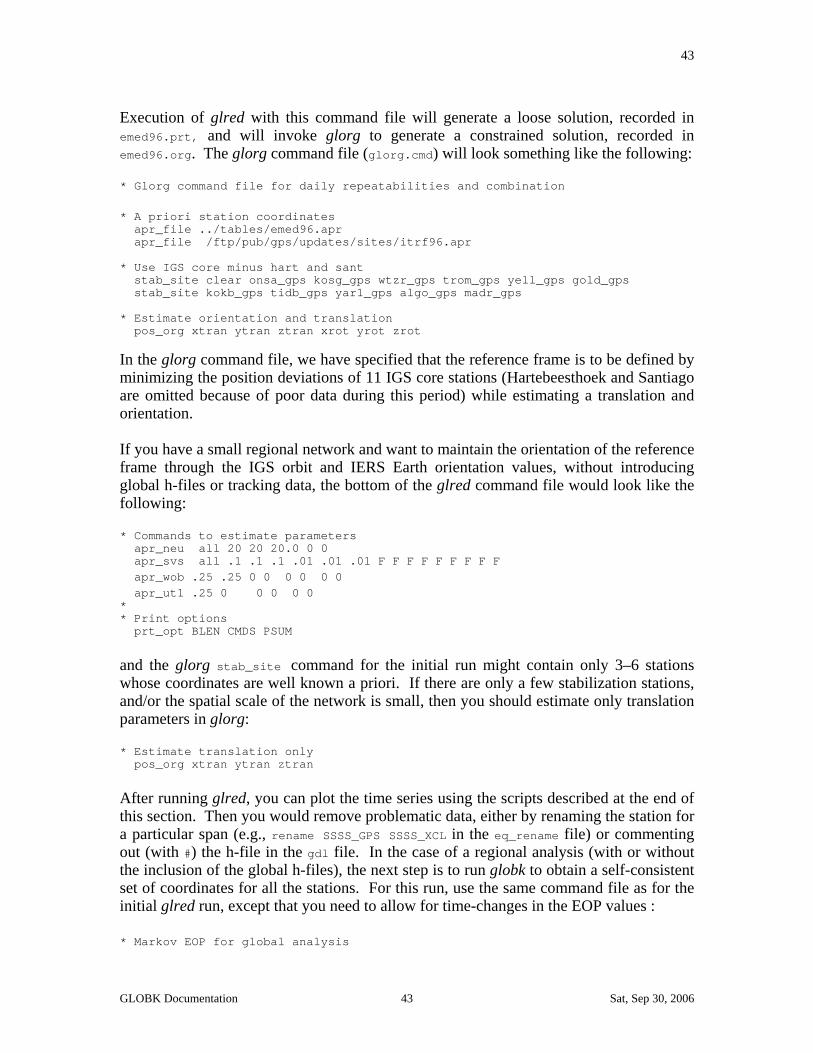
43

Execution of glred with this command file will generate a loose solution, recorded in emed96.prt, and will invoke glorg to generate a constrained solution, recorded in emed96.org. The glorg command file (glorg.cmd) will look something like the following: * Glorg command file for daily repeatabilities and combination

* A priori station coordinates apr_file ../tables/emed96.apr apr_file /ftp/pub/gps/updates/sites/itrf96.apr * Use IGS core minus hart and sant stab_site clear onsa_gps kosg_gps wtzr_gps trom_gps yell_gps gold_gps stab_site kokb_gps tidb_gps yar1_gps algo_gps madr_gps * Estimate orientation and translation pos_org xtran ytran ztran xrot yrot zrot

In the glorg command file, we have specified that the reference frame is to be defined by minimizing the position deviations of 11 IGS core stations (Hartebeesthoek and Santiago are omitted because of poor data during this period) while estimating a translation and orientation. If you have a small regional network and want to maintain the orientation of the reference frame through the IGS orbit and IERS Earth orientation values, without introducing global h-files or tracking data, the bottom of the glred command file would look like the following: * Commands to estimate parameters apr_neu all 20 20 20.0 0 0 apr_svs all .1 .1 .1 .01 .01 .01 F F F F F F F F F apr_wob .25 .25 0 0 0 0 0 0 apr_ut1 .25 0 0 0 0 0 * * Print options prt_opt BLEN CMDS PSUM

and the glorg stab_site command for the initial run might contain only 3–6 stations whose coordinates are well known a priori. If there are only a few stabilization stations, and/or the spatial scale of the network is small, then you should estimate only translation parameters in glorg: * Estimate translation only pos_org xtran ytran ztran After running glred, you can plot the time series using the scripts described at the end of this section. Then you would remove problematic data, either by renaming the station for a particular span (e.g., rename SSSS_GPS SSSS_XCL in the eq_rename file) or commenting out (with #) the h-file in the gdl file. In the case of a regional analysis (with or without the inclusion of the global h-files), the next step is to run globk to obtain a self-consistent set of coordinates for all the stations. For this run, use the same command file as for the initial glred run, except that you need to allow for time-changes in the EOP values : * Markov EOP for global analysis


44

x mar_wob 36500 36500 365 365 0 0 0 0 x mar_ut1 36500 365 0 0 0 0 * Markov EOP for regional analysis mar_wob 22.8 22.8 3.65 3.65 0 0 0 0 mar_ut1 22.8 3.65 0 0 0 0

If time span is longer than a single survey, you may also need to estimate a velocity for each of the stations: apr_neu all 20 20 20 1 1 1

After inspecting the globk run for consistency (chi-square values in the log file and rms of the glorg stabilization), you should now extract the coordinates for a new apr file from the glorg print file using grep 'Unc.' as described in Section 2.2. This new apr file will become the sole reference in glorg for the glred runs to generate the final time series (it doesn't matter what apr file you use in the glred command file). For this run, the glred command file will be the same as before, but the glorg command file will look like the following: * Glorg command file for daily repeatabilities and combination

* A priori station coordinates apr_file ../tables/soln_emed96.apr * Use IGS core minus hart and sant stab_site all stab_site -marm * Estimate translation only pos_org xtran ytran ztran

To plot coordinate repeatabilities from your glred solutions for a single survey using GMT, execute sh_plotcrd -f globk_rep.org

This script scans the solution file (globk_rep.org) for the north, east, and up coordinates estimated for each day and produces time series for each of the stations and a pair of histograms showing the distribution of weighted and normalized rms repeatabilities. If the data extend over several years, then you should specify -s long to have a trend removed and the horizontal axis labled in years rather than days. The programs and shell scripts called by sh_plotcrd, and that you can run individually to customize your time-series plots, are described in Chapter 4. Since the script creates a large number of files (one per station), you may want to execute it in a seperate (e.g., ../plots) directory and reference the input file by path (e.g., -f ../soln/globk_rep.org.) Estimating repeatabilities and velocities from several surveys Multi-year solutions are best accomplished by first combining the h-files from individual sessions into a single h-file. This is not only more efficient in terms of processing time


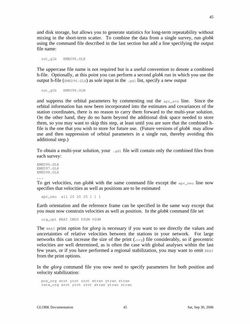
45

and disk storage, but allows you to generate statistics for long-term repeatability without mixing in the short-term scatter. To combine the data from a single survey, run globk using the command file described in the last section but add a line specifying the output file name: out_glb EMED96.GLX

The uppercase file name is not required but is a useful convention to denote a combined h-file. Optionally, at this point you can perform a second globk run in which you use the output h-file (EMED96.GLX) as sole input in the .gdl list, specify a new output out_glb EMED96.GLN

and suppress the orbital parameters by commenting out the apr_svs line. Since the orbital information has now been incorporated into the estimates and covariances of the station coordinates, there is no reason to carry them forward to the multi-year solution. On the other hand, they do no harm beyond the additional disk space needed to store them, so you may want to skip this step, at least until you are sure that the combined h-file is the one that you wish to store for future use. (Future versions of globk may allow use and then suppression of orbital parameters in a single run, thereby avoiding this additional step.) To obtain a multi-year solution, your .gdl file will contain only the combined files from each survey: EMED96.GLX EMED97.GLX EMED98.GLX . . . To get velocities, run globk with the same command file except the apr_neu line now specifies that velocities as well as positions are to be estimated apr_neu all 20 20 20 1 1 1

Earth orientation and the reference frame can be specified in the same way except that you must now constrain velocities as well as position. In the globk command file set org_opt BRAT CMDS PSUM VSUM

The BRAT print option for glorg is necessary if you want to see directly the values and uncertainties of relative velocities between the stations in your network. For large networks this can increase the size of the print (.org) file considerably, so if geocentric velocities are well determined, as is often the case with global analyses within the last few years, or if you have performed a regional stabilization, you may want to omit BRAT from the print options. In the glorg command file you now need to specify parameters for both position and velocity stabilization: pos_org xrot yrot zrot xtran ytran ztran rate_org xrot yrot zrot xtran ytran ztran


46

To create a velocity map from your solution ( e.g. globk_vel.org ), execute sh_plotvel -f globk_vel.org -maxsigma 5

where maxsigma gives maximum uncertainty in millimeters of sites to plot. Chapter 4 and the on-line help describe additional options for sh_plotvel that will allow you to produce journal-quality velocity maps including topography, tectonic features, and customized labels. Use of stochastic noise for stations and orbits There are a variety of reasons why you may want to treat station coordinates, orbital parameters, and Earth orientation parameters stochastically in your globk analysis. The classic method for analyzing the day-to-day or year-to-year variability of station coordinates or baseline components is to treat a subset of them stochastically and run both a forward and backward Kalman filter with the data. By performing both the forward and back solution, you obtain the best estimates of the coordinates and velocities of the stations treated deterministically at the same time as obtaining the variability of the stations treated stochastically. This approach has several disadvantages, however. The most obvious is the difficulty of deciding which stations to make deterministic and which to make stochastic. To retain nearly the full strength of the velocity solution, you would want to make only a few stations stochastic at a time, requiring many runs to see all of the repeatabilities. On the other hand, making deterministic a station for which there are outliers corrupts the solution and the apparent repeatability of other stations. A better approach to determining repeatabilities is to use glred to estimate all coordinates independently for each session or survey, with the reference frame maintained by glorg stabilization with as many stations as possible, as discussed in the previous section. With this approach the network can translate and rotate from solution to solution, but any internal distortions represent real problems with the stations exhibiting them. A more common current use of stochastic station coordinates is to account for time-correlated sources of error in the estimates of station position, including monument instability and signatures in global time series that may be due to errors in modeling the orbits or atmosphere. For example, to include random-walk noise at the level of 2 mm⎟yr in the horizontal coordinates, the globk command file entry would be mar_neu all 4.e-6 4.e-6 0 0 0 0

Prior to globk 5.05, Markov noise was also used to decouple erratic fluctuations in the estimates of vertical coordinates due to tropospheric noise, antenna changes, or blunders in entering the height of the antenna. The time-dependent nature of Markov noise makes it a poor proxy for these fluctuations, however. A better approach is to add random noise to the height estimates via the (new) neu_sig command. For example, to allow for 10 cm fluctuations in the vertical component for Kokee Park, the entry would be neu_sig kokb 0 0 .10


47

(If there are identifiable steps in the estimate of heights, you should rename the station at the time of the step [e.g., rename KOKB_GPS KOKB_APS] then equate the horizontal but not the vertical coordinate adjustments in glorg.) UT1 and pole position are defined as single (global) parameters in globk, so to allow day-to-day variation you must specify for them a Markov process. The level of constraint depends on the precision and stability of your a priori Earth rotation series as described in Section 3.3. For orbital parameters, stochastic variations are used in conjunction with multi-day arcs, most valuable prior to 1994 when the global tracking network was not strong enough to produce few part-per-billion orbital accuracy from a single day's observations. There is considerable flexibility in globk's use of stochastic parameters for orbits, allowing different levels of Markov constraint for each element of each satellite for each survey period. The difficulty, however, is determining in an efficient and objective manner what level to use. The analyst is forced to experiment with different values, using the chi-square increments between days from a globk non-stochastic forward solution and the day-to-day variations of the parameter estimates from a glred or back solution as a guide to choosing the optimal values. As a starting point, we discuss three levels, which we will designate "loose", "moderate", and "tight" orbital Markov constraints. "Loose" constraints would allow about 10 m/day (36500 m2/yr) variation in satellite initial position and 1 mm/s/day ( 365 (mm/s)2/yr) variation in initial velocity, and 2–100 %/day (0.15–365 /yr) variation in non-gravitational ("radiation-pressure") parameters: mar_svs all 36500 36500 36500 365 365 365 mar_rad all 365 365 .15 .15 .15 .15 .15 .15 .15

Remember that "loose" is defined with respect to the uncertainties you would obtain with a single-day's data with your actual data set, so these values can only be considered a guide. More study is needed to determine the relative weighting of initial conditions and non-gravitational-acceleration parameters to absorb a given degree of mis-modeling of the satellites' motion. In the example shown, we have allowed a relatively large "reset" of initial conditions each day, a large adjustment of the direct-radiation and y-bias parameters, and only a small (2%) change in the other non-gravitational acceleration parameters (the constant along the "B" axis and the once-per-rev coefficients in the Berne model; see Section 7.2 of the GAMIT manual). An alternate strategy would be to keep the initial condition variations small but allow large variations in all of the non-gravitational acceleration parameters. Values of the Markov constraints much looser than the ones shown here would completely decouple the orbits from day to day, effectively estimating the orbital motion in single-day arcs even though you have formally used a multi-day T-file with a single set of initial conditions. With loose Markov parameters for the orbits, if you are combining more than one h-file for each day (e.g., with regional and global observations), it is essential in this case to have the centers of the h-file data spans (the center of the X-file) match. Otherwise, you will decouple the orbital parameters estimated from the two h-files.


48

An example of "moderate" constraints would allow variations of 1 m/day (365 m2/yr), 0.1 m/s/day (3.65 (mm/s)2/yr), and 2–10 %/day (0.15–3.65 /yr) in initial position, initial velocity, and non-gravitational acceleration: mar_svs all 365 365 365 3.65 3.65 3.65 mar_rad all 3.65 3.65 .15 .15 .15 .15 .15 .15 .15 An example of "tight" constraints would allow variations of 0.1 m/day (3.65 m2/yr), .01 mm/s/day (0.0365 (mm/s)2/yr), and 1 %/day (.0365 /yr) in the orbital parameters: mar_svs all 3.65 3.65 3.65 .0365 .0365 .0365 mar_rad all .04 .04 .04 .04 .04 .04 .04 .04 .04

To invoke the Markov process for an individual satellite the command is, e.g., mar_svs prn_02 3.65 3.65 3.65 .0365 .0365 .0365 mar_rad prn_02 .04 .04 .04 .04 .04 .04 .04 .04 .04

You can allow different values to be applied for different period of time by specifying in the globk command file an auxiliary file: svs_marf svs.emed_markov

where svs.emed_markov is the name of file, and it contains, e.g., * YY MM DD HR Dur PRN * (days) 94 9 12 6 5 PRN_02 3.65 3.65 3.65 .04 .04 .04 .04 .04 .04 .04 .04 .04 .04 .04 .04 94 10 1 0 10 PRN_02 365 365 365 3.65 3.65 3.65 3.65 3.65 .04 .04 .04 .04 .04 .04 .04 94 10 2 0 5 PRN_05 365 365 365 3.65 3.65 3.65 3.65 3.65 .04 .04 .04 .04 .04 .04 .04

where Dur is the duration in days over which this alternative set of Markov parameters should apply. As many as entries as desired can be put into the file. Use of apr files in globk and glorg The rules and requirements for setting a priori coordinates and velocities in GAMIT and GLOBK analyses can be quite confusing because the needs are different at different stages and in different contexts. The most important concept to keep in mind is that reliable estimation of precise coordinates from both the phase data (GAMIT/solve) and loosely constrained coordinates and their covariances (globk or glorg) assumes that the adjustment from the (original, GAMIT) a priori is “small”, that is that there is insignificant non-linearity in the adjustments. Just how small the adjustment of a particular parameter needs to be depends on the functional dependence of the parameter and its correlation with other parameters. A conservative assumption for station coordinates is a convergence rate of 1:1000; that is., the adjustments need to be less than 0.5 m to achieve 0.5 mm precision in the estimated value. Hence, it is imperative that you iterate your phase solution (using, for example, the AUTCLN Postfit = R option in the GAMIT sestbl.) so that the a priori used for the solution written into the H-file differs from the final estimate by no more than a few decimeters.


49

If you use decimeter-level coordinates in GAMIT and are performing a straightforward globk/glorg solution from single-day H-files, it should not be necessary to include an apr file in the command files until you define your final coordinate frame, usually in glorg, and then the only sites that need to be included are those used in definiing the frame: if no a priori coordinates are input for a site, globk and glorg will use those passed from GAMIT via the h-file. However, there are several circumstances in which it is necessary to use an apr file. One of these occurs when you are combining daily h-files spanning many to average out the short-term noise before generating time series or estimating velocities. If a station has significant motion over this period, it is important to account for it in estimating the average position. You can do this by including an apr file that has a good a priori velocity for the station. Another time an apr file is helpful is when you plan to equate the positions of a station before and after an earthquake, after applying a model for the displacement. The glorg feature that assigns coordinates for a renamed site from the original site name, and the (new) FIXA option that forces the values of equated parameters to be the same, together make the explicit inclusion of an apr file usually not necessary, but there are circumstances when the logic may not work completely as you expect. Including an apr file can keep things clean. There are two utilities that are quite helpful in handling a priori coordinates. The first is glist (see Section 5.1) which will check the a priori coordinates for sites in each h-file in a gdl list with those from the first file in which the site appears, or with thosse from a specified apr file. For (and many other reasons) you should always run glist before running glred or globk. The second helpful utility is unify_apr, which alllows you to merge apr files while reconciling velocities of renamed or nearby sites so that they are all the same in an output apr file. 3.5 Examples of globk and glorg output There are two types of output produced in running globk/glred. The first is the "log" file, which contains the effect on the solution (usually loosely constrained) as each new h-file is added. The second is the "print" file, generated also by glorg, which contains the estimated parameter values. To illustrate the interpretation of these output files, we use as examples first the combination of regional and global data for a 10-day survey in the Salton Trough / Riverside County ("STRC") region of southern California from March, 1991, and then its combination with data from other GPS surveys and VLBI observations acquired between 1984 and 1997. The log file for the STRC91 survey is shown below. Because the global tracking network was sparse in 1991, it is particularly advantageous to estimate initial conditions and parameters of the GPS orbits by combining the data from several days. In this case, we estimated parameters for three overlapping arcs, each using data from 4 or 5 (24-hr) days. Within each arc we allowed the initial conditions and radiation-pressure parameters to have stochastic (Markov) variations from day to day. This scheme is illustrated by the grouping of h-files in the log file below, in which we have combined h-files representing 24 hrs of global data and 10 hrs (20:44-08:40 UTC) of regional data. The first orbital arc


50

(GAMIT T-file) spanned days 66–69 (7–11 March) with IC epoch 12h UTC on day 67 (year 91.1814). Data used to estimate the initial conditions and parameters included global data (h-files named _glob with the mid-point time 11:59) from days 66–69 and 10-hr regional data (h-files named _strc with mid-point time 02:43) from days 66–68 (the latter ending at 08:40 on day 69). Updating SV ephemeris epoch by 91.1814 years Global 1 using 3.7 Mb. Running time 2.00 Scaling by 1.000 1.00000000 For mgloba.066 Glbf ../glbf/glob1/h9103071159_glob.glr Chi**2 NP 249 is 0.370 Orient_adj. (mas) 1991 3 7 0.50 91.25 -0.46 92.29 0.8 94.48 Global 2 using 2.9 Mb. Running time 8.00 Scaling by 1.000 1.00000000 For mstrca.066 Glbf ../glbf/local/h9103080243_strc.glx Chi**2 NP 177 is 0.293 Orient_adj. (mas) 1991 3 8 -1.95 88.15 -3.07 84.33 2.2 91.33 Global 3 using 3.7 Mb. Running time 11.00 Scaling by 1.000 1.00000000 For mgloba.067 Glbf ../glbf/glob1/h9103081159_glob.glr Chi**2 NP 249 is 1.094 Orient_adj. (mas) 1991 3 8 -3.39 86.86 6.81 82.66 -4.2 90.48 Global 4 using 3.0 Mb. Running time 17.00 Scaling by 1.000 1.00000000 For mstrca.067 Glbf ../glbf/local/h9103090243_strc.glx Chi**2 NP 183 is 0.603 Orient_adj. (mas) 1991 3 9 0.91 85.37 -6.22 78.47 -2.3 89.08 Global 5 using 3.8 Mb. Running time 21.00 Scaling by 1.000 1.00000000 For mgloba.068 Glbf ../glbf/glob1/h9103091159_glob.glr Chi**2 NP 258 is 0.902 Orient_adj. (mas) 1991 3 9 1.55 83.62 -4.13 77.46 -8.0 88.43 Global 6 using 2.9 Mb. Running time 26.00 Scaling by 1.000 1.00000000 For mstrca.068 Glbf ../glbf/local/h9103100243_strc.glx Chi**2 NP 168 is 1.110 Orient_adj. (mas) 1991 3 10 1.10 82.96 -5.79 75.64 -11.2 87.87 Global 7 using 3.8 Mb. Running time 30.00 Scaling by 1.000 1.00000000 For mgloba.069 Glbf ../glbf/glob1/h9103101057_glob.glr Chi**2 NP 258 is 0.696 Updating SV ephemeris epoch by 0.0082 years Global 8 using 3.8 Mb. Running time 36.00 Scaling by 1.000 1.00000000 For mgloba.069 Glbf ../glbf/glob2/h9103101159_glob.glr Chi**2 NP 258 is 0.428 Orient_adj. (mas) 1991 3 10 0.19 81.73 -4.11 74.75 -5.8 84.78 Global 9 using 2.9 Mb. Running time 41.00 Scaling by 1.500 1.00000000 For mstrca.069 Glbf ../glbf/local/h9103110243_strc.glx Chi**2 NP 171 is 0.836 Orient_adj. (mas) 1991 3 11 -0.16 77.23 -4.98 70.60 -6.8 73.90 ... Global 14 using 3.5 Mb. Running time 66.00 Scaling by 1.000 1.00000000 For mgloba.072 Glbf ../glbf/glob2/h9103131057_glob.glr Chi**2 NP 234 is 0.756 Orient_adj. (mas) 1991 3 13 -0.45 75.35 -0.30 66.68 -12.4 72.16 Updating SV ephemeris epoch by 0.0110 years Global 15 using 3.5 Mb. Running time 71.00 Scaling by 1.000 1.00000000 For mgloba.072 Glbf ../glbf/glob3/h9103131159_glob.glr Chi**2 NP 237 is 0.375 Orient_adj. (mas) 1991 3 13 -4.27 74.06 -1.72 66.06 -4.4 68.84 Global 16 using 2.8 Mb. Running time 76.00 Scaling by 2.000 1.00000000 For mstrca.072 Glbf ../glbf/local/h9103140243_strc.glx Chi**2 NP 162 is 1.687 Orient_adj. (mas) 1991 3 14 -3.56 73.97 -1.19 65.76 -7.9 68.84 ... Global 23 using 3.1 Mb. Running time 109.00 Scaling by 1.000 1.00000000 For mgloba.076 Glbf ../glbf/glob3/h9103171159_glob.glr Chi**2 NP 198 is 1.884 Orient_adj. (mas) 1991 3 17 -2.08 72.17 3.15 62.62 1.0 66.71

There are three lines for each h-file used in the solution. The first gives the sequence number, size, run-time, and scale factors for the file. The second line is the most useful for evaluating the solution. It includes the GAMIT m-file name (which includes, conveniently, the day number), the binary h-file name (constructed from the GAMIT file name but with the date given as year, month, day, hour, minute), the number of parameters (NP) and the chi-square increment per degree of freedom when the data are added to the solution. If no tight constraints have been placed on the a priori values of the parameters, the first file should have a small chi-square value. As subsequent data are added, the values will increase to reflect the level of incompatibility between the newly added data and the solution from data previously included (see Dong et al., [1998] for the formulas used and a detailed discussion). An anomalously large chi-square increment in the log file is the most obvious indication that you have included erratic or poorly modeled data in your solution. If this occurs you should either omit the h-file (by commenting it out in the .gdl file) or return to the phase processing to find the source of the problem. If there is a consistent incompatibility between the global and regional h-files, there may be a model inconsistency between the two analyses (e.g., different antenna heights or antenna phase-


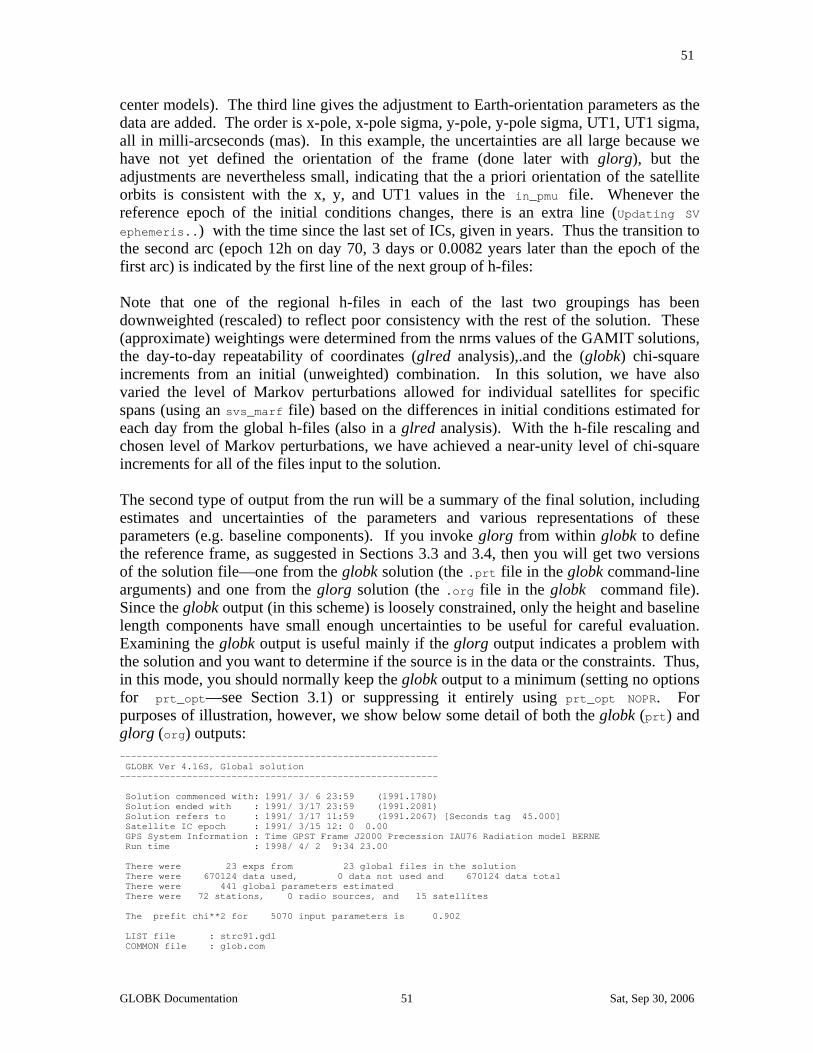
51

center models). The third line gives the adjustment to Earth-orientation parameters as the data are added. The order is x-pole, x-pole sigma, y-pole, y-pole sigma, UT1, UT1 sigma, all in milli-arcseconds (mas). In this example, the uncertainties are all large because we have not yet defined the orientation of the frame (done later with glorg), but the adjustments are nevertheless small, indicating that the a priori orientation of the satellite orbits is consistent with the x, y, and UT1 values in the in_pmu file. Whenever the reference epoch of the initial conditions changes, there is an extra line (Updating SV ephemeris..) with the time since the last set of ICs, given in years. Thus the transition to the second arc (epoch 12h on day 70, 3 days or 0.0082 years later than the epoch of the first arc) is indicated by the first line of the next group of h-files: Note that one of the regional h-files in each of the last two groupings has been downweighted (rescaled) to reflect poor consistency with the rest of the solution. These (approximate) weightings were determined from the nrms values of the GAMIT solutions, the day-to-day repeatability of coordinates (glred analysis),.and the (globk) chi-square increments from an initial (unweighted) combination. In this solution, we have also varied the level of Markov perturbations allowed for individual satellites for specific spans (using an svs_marf file) based on the differences in initial conditions estimated for each day from the global h-files (also in a glred analysis). With the h-file rescaling and chosen level of Markov perturbations, we have achieved a near-unity level of chi-square increments for all of the files input to the solution. The second type of output from the run will be a summary of the final solution, including estimates and uncertainties of the parameters and various representations of these parameters (e.g. baseline components). If you invoke glorg from within globk to define the reference frame, as suggested in Sections 3.3 and 3.4, then you will get two versions of the solution file—one from the globk solution (the .prt file in the globk command-line arguments) and one from the glorg solution (the .org file in the globk command file). Since the globk output (in this scheme) is loosely constrained, only the height and baseline length components have small enough uncertainties to be useful for careful evaluation. Examining the globk output is useful mainly if the glorg output indicates a problem with the solution and you want to determine if the source is in the data or the constraints. Thus, in this mode, you should normally keep the globk output to a minimum (setting no options for prt_opt—see Section 3.1) or suppressing it entirely using prt_opt NOPR. For purposes of illustration, however, we show below some detail of both the globk (prt) and glorg (org) outputs: --------------------------------------------------------- GLOBK Ver 4.16S, Global solution --------------------------------------------------------- Solution commenced with: 1991/ 3/ 6 23:59 (1991.1780) Solution ended with : 1991/ 3/17 23:59 (1991.2081) Solution refers to : 1991/ 3/17 11:59 (1991.2067) [Seconds tag 45.000] Satellite IC epoch : 1991/ 3/15 12: 0 0.00 GPS System Information : Time GPST Frame J2000 Precession IAU76 Radiation model BERNE Run time : 1998/ 4/ 2 9:34 23.00 There were 23 exps from 23 global files in the solution There were 670124 data used, 0 data not used and 670124 data total There were 441 global parameters estimated There were 72 stations, 0 radio sources, and 15 satellites The prefit chi**2 for 5070 input parameters is 0.902 LIST file : strc91.gdl COMMON file : glob.com


52

MARKOV file : globk_cmb.cmd GLORG CMD file : glorg.cmd APRIORI file : /data8/rwk/scec_pre/soln/preland_nafd.apr NUTATION file : PLANETARY file : SD ORIENT file : PMU file : /data3/tah/tables/vlbi_84.1_95.11.dat BACK SOLN file : OUTGLOBAL file : strc91.glx SVS EPHEM file : ../../tables/sat.apr:A SVS MARKOV file: ../gsoln/svs.mar EARTHQUAKE file: /data9/ftp/pub/gps/scec/scec_eq_v1.5 There were 205 site renames applied # Orig New Specific Period from -----> To Position change (m) Type 1 WETT_GPS->WETI_GPS 1987/11/12 0: 0 1989/ 7/23 0: 0 0.0000 0.0000 0.0000 XYZ 2 RIC1_GPS->RICM_GPS 1989/ 2/ 5 0: 0 1992/12/31 0: 0 0.0000 0.0000 0.0000 XYZ 3 WES1_GPS->WSFM_GPS 1989/ 2/ 5 0: 0 1999/12/31 0: 0 0.0000 0.0000 0.0000 XYZ 4 TSUK_GPS->TSU1_GPS 1988/ 7/10 0: 0 1991/12/17 0: 0 0.0000 0.0000 0.0000 XYZ 5 TSU0_GPS->TSU1_GPS 1989/11/ 9 0: 0 1989/11/28 0: 0 0.0000 0.0000 0.0000 XYZ ... 204 MAYO_GPS->MAYR_GPS 1997/ 3/ 3 0: 0 1997/ 3/20 0: 0 0.0000 0.0000 0.0000 XYZ 205 USUD_GPS->USUD_DUP 1997/ 1/ 6 0: 0 1997/ 8/24 0: 0 0.0000 0.0000 0.0000 XYZ There were 2 earthquakes # CODE Lat (deg) Long (deg) Radius (km) Depth (km) Date Rename? 1 LA 34.4500 243.5000 500.0000 20.0000 1992/ 6/28 12: 0 YES 2 NR 34.2800 241.4400 150.0000 9.7200 1994/ 1/17 12:31 YES COSEISMIC characteristics # CODE Static sigma Spatial Sigma (Depth/Dist)^2 North East Height (m) North East Height (m) 1 LA 1.0000 1.0000 1.0000 1.8000 1.8000 0.7000 2 NR 1.0000 1.0000 1.0000 1.8000 1.8000 0.7000 PRE-SEISMIC characteristics # CODE Dur Static Process Spatial Process (Depth/Dist)^2 (days) North East Height North East Height (mm^2/day) (mm^2/day) 1 LA 0.0 0.0000 0.0000 0.0000 0.0000 0.0000 0.0000 2 NR 0.0 0.0000 0.0000 0.0000 0.0000 0.0000 0.0000 POST-SEISMIC characteristics # CODE Dur Static Process Spatial Process (Depth/Dist)^2 (days) North East Height North East Height (mm^2/day) (mm^2/day) 1 LA 0.0 0.1000 0.1000 0.1000 1.8000 1.8000 0.7000 2 NR 0.0 0.1000 0.1000 0.1000 1.8000 1.8000 0.7000 SITES WITH NO UPDATED APRIORI COORDINATES: ENDD_GPS 1109_GPS SAND_GPS DS40_GPS ANKT_GPS Summary of Markov file globk_cmb.cmd ------------------------------------------------------------------------------- * GLOBK command file for combining STRC regionals with multiday orbits * This version uses loose constraints all stations to get output combined file make_svs ../../tables/sat.apr * earthquake and site rename eq_file /data9/ftp/pub/gps/scec/scec_eq_v1.5 com_file glob.com srt_file glob.srt out_glb strc91.glx * Station apr files apr_file /data8/rwk/scec_pre/soln/preland_nafd.apr in_pmu /data3/tah/tables/vlbi_84.1_95.11.dat max_chii 100. 10000. desc STRC91 combination with multi-day stochastic orbits prt_opt CMDS GDLF * select the stations you want to retain in the solution * keep all for these solutions use_site clear all *Loose here--for combination apr_neu all 20.0 20.0 20.0 0 0 0 * Markov height for mojm and wetm to accout for 10 cm / 1.5 m height error between GIG ties and strc * --allow 4 m**2/0.1 yr or 40 m**2/yr mar_neu mojm 0 0 40 0 0 0 mar_neu wetm 0 0 40 0 0 0 * Estimate translation and scale explicitly -- not needed: see notes 970826 * Loosely constrain all satellite initial condition parameters * X Y Z XDOT YDOT ZDOT DRAD YRAD ZRAD BRAD XRAD DCOS DSIN YCOS YSIN BCOS BSIN apr_svs all 100 100 100 10 10 10 1. 1. F 1.0 F 0.05 0.05 0.05 0.05 0.05 0.05 mar_svs all 3.65 3.65 3.65 .0365 .0365 .0365 mar_rad all .01 .01 .01 .01 .01 .01 .01 .01 .01 svs_marf ../gsoln/svs.mar * For a small network, constrain EOP with the IERS values to 0.25 mas, 0.1 mas/day * Network is global but weak, so keep tight constraints


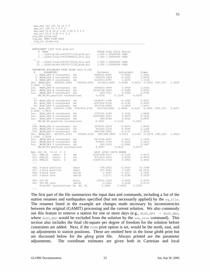
53

apr_wob 100 100 10 10 0 0 apr_ut1 100 10 0 0 0 0 mar_wob 22.8 22.8 3.65 3.65 0 0 0 0 mar_ut1 22.8 3.65 0 0 0 0 org_cmd glorg.cmd org_opt CMDS PSUM GDLF org_out glred.org ------------------------------------------------------------------------------- EXPERIMENT LIST from glob.srt # Name SCALE Diag Scale Status 1 ../glbf/glob1/h9103071159_glob.glr 1.000 1.00000000 USED 2 ../glbf/local/h9103080243_strc.glx 1.000 1.00000000 USED ... 22 ../glbf/local/h9103170243_strc.glx 1.000 1.00000000 USED 23 ../glbf/glob3/h9103171159_glob.glr 1.000 1.00000000 USED PARAMETER ESTIMATES FROM GLOBK Vers 4.16S # PARAMETER Estimate Adjustment Sigma 1. MADR_GPS X coordinate (m) 4849202.4060 -0.0849 1.3602 2. MADR_GPS Y coordinate (m) -360329.5954 -0.3645 2.0938 3. MADR_GPS Z coordinate (m) 4114913.4997 0.4670 1.7218 Unc. MADR_GPS 4849202.4060 -360329.5954 4114913.4997 0.0096 0.0219 -0.0034 1991.207 1.3602 2.0938 1.7218 Loc. MADR_GPS N coordinate (m) 4500553.9009 0.3929 2.2526 Loc. MADR_GPS E coordinate (m) 30144706.2943 -0.3698 2.0295 Loc. MADR_GPS U coordinate (m) 829.7021 0.2589 0.0746 NE,NU,EU position correlations 0.6318 0.1334 0.0530 ... 43. BLAC_GPS X coordinate (m) -2306307.1398 -0.1456 0.4557 44. BLAC_GPS Y coordinate (m) -4787914.6736 -0.3193 0.9200 45. BLAC_GPS Z coordinate (m) 3515736.8095 0.3829 1.5413 Unc. BLAC_GPS -2306307.1398 -4787914.6736 3515736.8095 0.0008 0.0107 -0.0045 1991.207 0.4557 0.9200 1.5413 Loc. BLAC_GPS N coordinate (m) 3747431.5165 0.1242 1.8469 Loc. BLAC_GPS E coordinate (m) 22632945.3672 0.0074 0.1222 Loc. BLAC_GPS U coordinate (m) 489.9158 0.5043 0.0597 NE,NU,EU position correlations -0.0021 0.1126 -0.0001 ... 208. WETM_GPS X coordinate (m) 4075551.8219 -0.6872 1.8916 209. WETM_GPS Y coordinate (m) 931825.2518 -0.4090 2.1268 210. WETM_GPS Z coordinate (m) 4801588.9993 -0.1141 1.4156 Unc. WETM_GPS 4075551.8219 931825.2518 4801588.9993 0.0012 0.0193 -0.0079 1991.207 1.8916 2.1268 1.4156 Loc. WETM_GPS N coordinate (m) 5470746.8267 0.5011 2.1440 Loc. WETM_GPS E coordinate (m) 937807.2799 -0.2456 2.3413 Loc. WETM_GPS U coordinate (m) 659.3243 -0.5842 0.1647 NE,NU,EU position correlations 0.4957 0.0610 0.0173 Eph. #IC 91 74 12 0 0 GPST J2000 IAU76 BERNE 211. PRN_02 Inert. X (m) 22367188.9177 -0.1123 2.8273 212. PRN_02 Inert. Y (m) 9712914.6475 0.2035 6.4919 213. PRN_02 Inert. Z (m) 11050733.3763 0.6933 0.3662 ... 436. X-pole position (mas) -199.2422 -2.0837 72.1698 437. Y-pole position (mas) 227.0541 3.1497 62.6152 438. X-pole rate (ms/d) -1.9267 -0.1917 0.1982 439. Y-pole rate (ms/d) 3.2171 -0.0188 0.2018 440. UT1-AT (mts) -25551.1550 0.0692 4.4475 441. UT1-AT rate (ms/d) -3.0222 0.0238 0.0733 Pole/UT1 correlations: XY, XU, YU 0.1664 0.4639 0.2534 ...

The first part of the file summarizes the input data and commands, including a list of the station renames and earthquakes specified (but not necessarily applied) by the eq_file. The renames listed in the example are changes made necessary by inconsistencies between the original (GAMIT) processing and the current solution. We also commonly use this feature to remove a station for one or more days (e.g., ALGO_GPS -> ALGO_BAD, where ALGO_BAD would be excluded from the solution by the use_site command). This section also includes the final chi-square per degree of freedom for the solution before constraints are added. Next, if the PSUM print option is set, would be the north, east, and up adjustments to station positions. These are omitted here in the loose globk print but are discussed below for the glorg print file. Always printed are the parameter adjustments. The coordinate estimates are given both in Cartesian and local


54

representation. Both here and in the station or baseline summary sections, the north and up adjustments are computed conventionally; i. e., north is the product of the adjustment in geodetic latitude by the semi-major axis of the ellipsoid (see kf/includes/const_param.h for ellipsoid definition) and up is the adjustment in geodetic height. The east adjustment, however, is unconventional: the adjustment in longitude (measured east from Greenwich) is multiplied by the radius of the small circle at the nearest 1 degree latitude line of the station. This scheme keeps the adjustment in the east value from being affected by changes in latitude. The estimates of orbital and Earth rotation parameters (EOPs) are self-explanatory, but note that in a globk solution to combine many days of data, in which new initial conditions and EOPs are estimated for each day, the estimates represent the solution from only the last day and are therefore of limited value. The final sections of the print file express the coordinate estimates in terms of baseline length and components. These appear only if BLEN has been set in prt_opt and are again omitted in this example.

Shown below is the glorg print file for the same run. It begins with a report of application of generalized constraints to establish the reference frame ("stabilization"). Recall that glorg is minimizing, in an iterative scheme, the departure from a priori values of the coordinates of a selected set of stations while estimating a rotation and translation of the frame. The first four lines echo the parameters used to decide whether a station is retained at each iteration of the stabilization scheme. The first line indicates that only 50% of the weight for a station may be altered in iteration, thus preventing the ratio of weights from becoming too high. The third line indicates that heights are downweighted by a factor of 10 relative to horizontal coordinates. The second line and the second column of the fourth line indicate that a station is removed if its residual becomes more than 4 times the rms of the fit (after application of relative weights) but not if its residual is within 12 mm (4 times the Min Position value of 3 mm). The first column of the fourth line establishes a floor for the ratio tolerance (2.0 here) used to remove a station which has a larger-than-average height uncertainty (see the cnd_hgtv command). Height sigma is used as the primary condition at the first iteration since the horizontal coordinates will not be well determined until after initial stabilization. STRC91 combination with multi-day stochastic orbits +++++++++++++++++++++++++++++++++++++ + GLORG Version 4.04S + +++++++++++++++++++++++++++++++++++++ Stabilization with 50.0% constant, 50.0% site dependent weighting. Delete sites with 4.0-sigma condition. Height variance factor 10.00 Position, 10.00 Velocity Min dH sigma Position 0.0050 m; Min Position RMS 0.0030 m Min dH sigma Velocity 0.0050 m/yr; Min Velocity RMS 0.0030 m/yr ========================================================================================================== Starting stabilization iteration 1 For 8 sites in origin, min/max height sigma 59.16 87.33 mm; Median 67.11 mm, Tol 7.94 mm Removing YELL_GPS from orgin condition, height sigma 87.33 mm, Ratio Tol 2.000 Position system stabilization results --------------------------------------- X Rotation (mas) 6.48985 +- 1.76907 Iter 1 Y Rotation (mas) 5.51514 +- 2.83950 Iter 1 Z Rotation (mas) -2.78903 +- 0.61673 Iter 1 X Translation (m) 0.04711 +- 0.04285 Iter 1 Y Translation (m) -0.40873 +- 0.05498 Iter 1 Z Translation (m) 0.30527 +- 0.04604 Iter 1 Condition Sigmas used 0.0000 0.0000 0.0000 0.0000 0.0000 0.0000 Sites and relative sigmas used in stabilization MADR_GPS 1.00 BLAC_GPS 1.00 OCOT_GPS 1.00 MONU_GPS 1.00 PIN2_GPS 1.00 MOJM_GPS 1.00


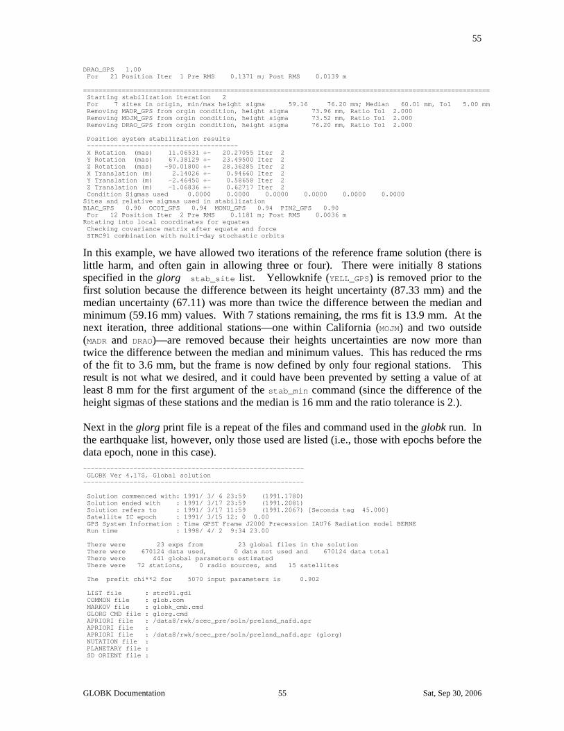
55

DRAO_GPS 1.00 For 21 Position Iter 1 Pre RMS 0.1371 m; Post RMS 0.0139 m ========================================================================================================= Starting stabilization iteration 2 For 7 sites in origin, min/max height sigma 59.16 76.20 mm; Median 60.01 mm, Tol 5.00 mm Removing MADR_GPS from orgin condition, height sigma 73.96 mm, Ratio Tol 2.000 Removing MOJM_GPS from orgin condition, height sigma 73.52 mm, Ratio Tol 2.000 Removing DRAO_GPS from orgin condition, height sigma 76.20 mm, Ratio Tol 2.000 Position system stabilization results --------------------------------------- X Rotation (mas) 11.06531 +- 20.27055 Iter 2 Y Rotation (mas) 67.38129 +- 23.49500 Iter 2 Z Rotation (mas) -90.01800 +- 28.36285 Iter 2 X Translation (m) 2.14026 +- 0.94660 Iter 2 Y Translation (m) -2.46450 +- 0.58658 Iter 2 Z Translation (m) -1.06836 +- 0.62717 Iter 2 Condition Sigmas used 0.0000 0.0000 0.0000 0.0000 0.0000 0.0000 Sites and relative sigmas used in stabilization BLAC_GPS 0.90 OCOT_GPS 0.94 MONU_GPS 0.94 PIN2_GPS 0.90 For 12 Position Iter 2 Pre RMS 0.1181 m; Post RMS 0.0036 m Rotating into local coordinates for equates Checking covariance matrix after equate and force STRC91 combination with multi-day stochastic orbits

In this example, we have allowed two iterations of the reference frame solution (there is little harm, and often gain in allowing three or four). There were initially 8 stations specified in the glorg stab_site list. Yellowknife (YELL_GPS) is removed prior to the first solution because the difference between its height uncertainty (87.33 mm) and the median uncertainty (67.11) was more than twice the difference between the median and minimum (59.16 mm) values. With 7 stations remaining, the rms fit is 13.9 mm. At the next iteration, three additional stations—one within California (MOJM) and two outside (MADR and DRAO)—are removed because their heights uncertainties are now more than twice the difference between the median and minimum values. This has reduced the rms of the fit to 3.6 mm, but the frame is now defined by only four regional stations. This result is not what we desired, and it could have been prevented by setting a value of at least 8 mm for the first argument of the stab_min command (since the difference of the height sigmas of these stations and the median is 16 mm and the ratio tolerance is 2.). Next in the glorg print file is a repeat of the files and command used in the globk run. In the earthquake list, however, only those used are listed (i.e., those with epochs before the data epoch, none in this case). --------------------------------------------------------- GLOBK Ver 4.17S, Global solution --------------------------------------------------------- Solution commenced with: 1991/ 3/ 6 23:59 (1991.1780) Solution ended with : 1991/ 3/17 23:59 (1991.2081) Solution refers to : 1991/ 3/17 11:59 (1991.2067) [Seconds tag 45.000] Satellite IC epoch : 1991/ 3/15 12: 0 0.00 GPS System Information : Time GPST Frame J2000 Precession IAU76 Radiation model BERNE Run time : 1998/ 4/ 2 9:34 23.00 There were 23 exps from 23 global files in the solution There were 670124 data used, 0 data not used and 670124 data total There were 441 global parameters estimated There were 72 stations, 0 radio sources, and 15 satellites The prefit chi**2 for 5070 input parameters is 0.902 LIST file : strc91.gdl COMMON file : glob.com MARKOV file : globk_cmb.cmd GLORG CMD file : glorg.cmd APRIORI file : /data8/rwk/scec_pre/soln/preland_nafd.apr APRIORI file : APRIORI file : /data8/rwk/scec_pre/soln/preland_nafd.apr (glorg) NUTATION file : PLANETARY file : SD ORIENT file :


56

PMU file : /data3/tah/tables/vlbi_84.1_95.11.dat BACK SOLN file : OUTGLOBAL file : strc91.glx SVS EPHEM file : ../../tables/sat.apr:A SVS MARKOV file: ../gsoln/svs.mar EARTHQUAKE file: /data9/ftp/pub/gps/scec/scec_eq_v1.5 There were 205 site renames listed. Renames used are: # Orig New Specific Period from -----> To Position change (m) Type 6 TSUK_GPS->TSU2_GPS 1991/12/17 0: 0 1993/12/15 0: 0 0.0000 0.0000 0.0000 XYZ 14 DS42_GPS->TIDB_GPS 1989/12/10 0: 0 1999/12/31 0: 0 0.0000 0.0000 0.0000 XYZ 22 JPL1_GPS->JPLM_GPS 1990/ 4/ 2 0: 0 1999/12/31 0: 0 0.0000 0.0000 0.0000 XYZ ... 182 MAYO_GPS->MAYR_GPS 1995/ 2/ 7 0: 0 1995/ 2/20 0: 0 0.0000 0.0000 0.0000 XYZ There were 2 earthquakes listed. Earthquakes used are: # CODE Lat (deg) Long (deg) Radius (km) Depth (km) Date Rename? SITES WITH NO UPDATED APRIORI COORDINATES: ENDD_GPS 1109_GPS SAND_GPS DS40_GPS ANKT_GPS Summary of Markov file globk_cmb.cmd ------------------------------------------------------------------------------- * GLOBK command file for combining STRC regionals with multiday orbits .. ------------------------------------------------------------------------------- EXPERIMENT LIST from glob.srt # Name SCALE Diag PPM Forw Chi2 Back Chi2 Status 1 ../glbf/glob1/h9103071159_glob.glr 1.000 0.000 0.375 -1.000 USED 2 ../glbf/local/h9103080243_strc.glx 1.000 0.000 0.293 -1.000 USED 3 ../glbf/glob1/h9103081159_glob.glr 1.000 0.000 1.077 -1.000 USED ... 23 ../glbf/glob3/h9103171159_glob.glr 1.000 0.000 1.884 -1.000 USED

For the glorg print we have specified PSUM as an option, so we get a more readable table of the adjustments and uncertainties of the east, north, and up coordinates for each station. This table is the most useful for evaluating the solution and contains the values later extracted by ensum (invoked by sh_globk_scatter) in order to generated statistics and plot station-coordinate repeatabilities. The column marked RHO in the coordinate adjustments (Rne in the baseline component estimates) gives the correlation between the north and east estimates; this is necessary to compute horizontal uncertainty ellipses. As elsewhere in globk, the stations are ordered by longitude, so that (usually) nearby stations are grouped together in the list: SUMMARY POSITION ESTIMATES FROM GLOBK Ver 4.17S Long. Lat. dE adj. dN adj. dE +- dN +- RHO dH adj. dH +- SITE (deg) (deg) (mm) (mm) (mm) (mm) (mm) (mm) 355.750 40.429 295.7 214.8 120.1 149.2 0.894 -182.4 48.7 MADR_GPS 288.507 42.613 3.3 329.1 13.1 109.0 0.125 -131.4 25.6 WSFM_GPS 279.616 25.614 105.6 308.3 40.5 90.8 0.954 5.2 19.2 RICM_GPS 245.519 62.481 -314.4 44.2 89.4 10.2 -0.468 -180.7 26.9 YELL_GPS 245.519 34.044 313.5 -147.7 5.3 5.9 -0.286 201.7 13.7 ENDD_GPS 245.193 30.931 18.1 3.7 10.9 4.9 0.614 81.4 16.1 SFBC_GPS 244.280 33.664 -2.4 3.5 0.8 1.6 0.128 21.5 2.4 BLAC_GPS* 244.236 33.834 -57.0 47.6 1.3 1.8 -0.104 290.3 7.2 JTRE_GPS 244.204 32.790 -2.3 -1.3 3.2 2.8 -0.438 -27.2 3.1 OCOT_GPS* 243.590 33.039 -49.1 38.9 3.5 2.7 0.123 315.9 12.9 SD16_GPS 243.577 32.892 0.0 2.3 2.7 1.9 -0.043 32.6 3.7 MONU_GPS* 243.569 33.870 -61.0 38.8 1.3 1.6 0.043 281.0 7.6 EDOM_GPS 243.542 33.612 4.5 -4.4 0.9 1.4 -0.527 -26.6 2.9 PIN2_GPS* 243.511 33.839 -60.8 34.3 1.2 1.7 0.016 284.5 6.5 PSAR_GPS ... 18.938 69.663 457.0 159.4 141.2 113.7 0.910 -270.5 50.1 TROM_GPS 12.879 49.145 494.5 202.6 144.6 127.7 0.877 -1082.8 151.8 WETM_GPS

The stations marked by an asterisk (*) are those used in stablization. Note that since the reference frame stabilization used only stations within California, only stations in this region (longitudes 243–245) have small horizontal uncertainties. Following the position summary is a list of all the parameter adjustments, as in the globk print file: PARAMETER ESTIMATES FROM GLOBK Vers 4.17S # PARAMETER Estimate Adjustment Sigma 1. MADR_GPS X coordinate (m) 4849202.2333 -0.2576 0.0881 2. MADR_GPS Y coordinate (m) -360328.9148 0.3161 0.1266


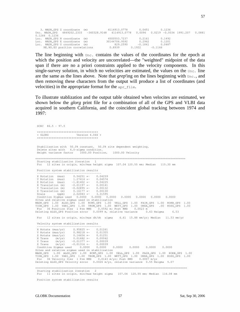
57

3. MADR_GPS Z coordinate (m) 4114913.0778 0.0451 0.1236 Unc. MADR_GPS 4849202.2333 -360328.9148 4114913.0778 0.0096 0.0219 -0.0034 1991.207 0.0881 0.1266 0.1236 Loc. MADR_GPS N coordinate (m) 4500553.7237 0.2161 0.1492 Loc. MADR_GPS E coordinate (m) 30144706.9592 0.2962 0.1201 Loc. MADR_GPS U coordinate (m) 829.2590 -0.1841 0.0487 NE,NU,EU position correlations 0.8939 0.1922 -0.1166

The line beginning with Unc. contains the values of the coordinates for the epoch at which the position and velocity are uncorrelated—the "weighted" midpoint of the data span if there are no a priori constraints applied to the velocity components. In this single-survey solution, in which no velocities are estimated, the values on the Unc. line are the same as the lines above. Note that grep'ing on the lines beginning with Unc., and then removing these characters from the output will produce a list of coordinates (and velocities) in the appropriate format for the apr_file. To illustrate stablization and the output table obtained when velocites are estimated, we shown below the glorg print file for a combination of all of the GPS and VLBI data acquired in southern California, and the coincident global tracking between 1974 and 1997: SCEC 86.5 - 97.5 +++++++++++++++++++++++++++++++++++++ + GLORG Version 4.04S + +++++++++++++++++++++++++++++++++++++ Stabilization with 50.0% constant, 50.0% site dependent weighting. Delete sites with 4.0-sigma condition. Height variance factor 1000.00 Position, 1000.00 Velocity =========================================================================================== Starting stabilization iteration 1 For 12 sites in origin, min/max height sigma 107.04 120.55 mm; Median 115.30 mm Position system stabilization results --------------------------------------- X Rotation (mas) 0.56251 +- 0.04259 Y Rotation (mas) 1.27414 +- 0.04574 Z Rotation (mas) -1.81402 +- 0.04225 X Translation (m) -0.01197 +- 0.00141 Y Translation (m) -0.02895 +- 0.00132 Z Translation (m) 0.16177 +- 0.00130 Scale (ppb) 2.02083 +- 3.31595 Condition Sigmas used 0.0000 0.0000 0.0000 0.0000 0.0000 0.0000 0.0000 Sites and relative sigmas used in stabilization MADR_GPS 1.00 ALGO_GPS 1.00 RCM5_GPS 1.00 YELL_GPS 1.00 FAIR_GPS 1.00 KOKB_GPS 1.00 TIDB_GPS 1.00 YAR1_GPS 1.00 TROM_GPS 1.00 WETT_GPS 1.00 ONSA_GPS .00 KOSG_GPS 1.00 For 36 Position Iter 1 Pre RMS 0.0592 m; Post RMS 0.0023 m Deleting ALGO_GPS Position error 0.0099 m, relative variance 0.43 Nsigma 6.53 For 12 sites in origin, min/max dh/dt sigma 6.61 15.88 mm/yr; Median 11.53 mm/yr Velocity system stabilization results --------------------------------------- X Rotate (mas/yr) 0.95825 +- 0.01261 Y Rotate (mas/yr) 0.98218 +- 0.01355 Z Rotate (mas/yr) 0.14656 +- 0.01251 X Trans (m/yr) 0.01682 +- 0.00042 Y Trans (m/yr) -0.01377 +- 0.00039 Z Trans (m/yr) -0.01316 +- 0.00039 Condition Sigmas used 0.0000 0.0000 0.0000 0.0000 0.0000 0.0000 Sites and relative sigmas used in stabilization MADR_GPS 1.00 ALGO_GPS 1.00 RCM5_GPS 1.00 YELL_GPS 1.00 FAIR_GPS 1.00 KOKB_GPS 1.00 TIDB_GPS 1.00 YAR1_GPS 1.00 TROM_GPS 1.00 WETT_GPS 1.00 ONSA_GPS 1.00 KOSG_GPS 1.00 For 36 Velocity Iter 1 Pre RMS 0.0143 m/yr; Post RMS 0.0007 m/yr Deleting ALGO_GPS Velocity error 0.0026 m/yr, relative variance 0.55 Nsigma 5.07 ============================================================================================ Starting stabilization iteration 2 For 11 sites in origin, min/max height sigma 107.04 120.55 mm; Median 116.08 mm Position system stabilization results


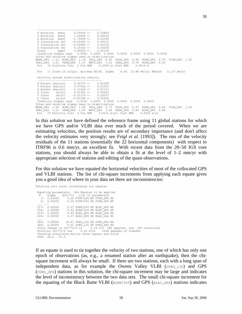
58

--------------------------------------- X Rotation (mas) 0.55654 +- 0.03806 Y Rotation (mas) 1.24449 +- 0.04249 Z Rotation (mas) -1.75096 +- 0.03390 X Translation (m) -0.01094 +- 0.00131 Y Translation (m) -0.02846 +- 0.00118 Z Translation (m) 0.16182 +- 0.00105 Scale (ppb) 3.90049 +- 2.62134 Condition Sigmas used 0.0000 0.0000 0.0000 0.0000 0.0000 0.0000 0.0000 Sites and relative sigmas used in stabilization MADR_GPS 1.12 RCM5_GPS 1.19 YELL_GPS 0.63 FAIR_GPS 0.94 KOKB_GPS 0.76 TIDB_GPS 1.25 YAR1_GPS 1.21 TROM_GPS 1.13 WETT_GPS 1.12 ONSA_GPS 0.78 KOSG_GPS 0.93 For 33 Position Iter 2 Pre RMS 0.0599 m; Post RMS 0.0019 m For 11 sites in origin, min/max dh/dt sigma 6.60 15.88 mm/yr; Median 11.67 mm/yr Velocity system stabilization results --------------------------------------- X Rotate (mas/yr) 0.95797 +- 0.01208 Y Rotate (mas/yr) 0.97666 +- 0.01353 Z Rotate (mas/yr) 0.13164 +- 0.01101 X Trans (m/yr) 0.01652 +- 0.00042 Y Trans (m/yr) -0.01376 +- 0.00037 Z Trans (m/yr) -0.01299 +- 0.00034 Condition Sigmas used 0.0000 0.0000 0.0000 0.0000 0.0000 0.0000 Sites and relative sigmas used in stabilization MADR_GPS 1.06 RCM5_GPS 1.09 YELL_GPS 0.73 FAIR_GPS 0.97 KOKB_GPS 0.84 TIDB_GPS 1.24 YAR1_GPS 1.21 TROM_GPS 1.07 WETT_GPS 1.06 ONSA_GPS 0.86 KOSG_GPS 0.98 For 33 Velocity Iter 2 Pre RMS 0.0131 m/yr; Post RMS 0.0006 m/yr

In this solution we have defined the reference frame using 11 global stations for which we have GPS and/or VLBI data over much of the period covered. When we are estimating velocities, the position results are of secondary importance (and don't affect the velocity estimates very strongly; see Feigl et al. [1993]). The rms of the velocity residuals of the 11 stations (essentially the 22 horizontal components) with respect to ITRF96 is 0.6 mm/yr, an excellent fit. With recent data from the 20–50 IGS core stations, you should always be able to obtain a fit at the level of 1–2 mm/yr with appropriate selection of stations and editing of the quasi-observations. For this solution we have equated the horizontal velocities of most of the collocated GPS and VLBI stations. The list of chi-square increments from applying each equate gives you a good idea of where in your data set there are inconsistencies: Rotating into local coordinates for equates Equating parameters: 384 Equates to be applied # Sigma dChi**2 List of parameters 1: 0.02000 0.00 FTOR7266 NP FTOR_GPS NP 2: 0.02000 0.30 FTOR7266 EP FTOR_GPS EP ... ... 217: 0.00000 0.37 BLKB7269 ND BLAC_GPS ND 218: 0.00000 0.42 BLKB7269 ED BLAC_GPS ED 219: 0.00000 0.42 BLAC_GPS ND BLAC_GLA ND 220: 0.00000 3.57 BLAC_GPS ED BLAC_GLA ED ... 383: 0.00000 18.61 OVRO_130 ND OVRO_GPS ND 384: 0.00000 0.01 OVRO_130 ED OVRO_GPS ED Total change in Chi**2/f is 2.19 for 384 equates, and 392 conditions Solution chi**2/f now 0.44 with 2228 degrees of freedom Checking covariance matrix after equate and force SCEC 86.5 - 97.5

If an equate is used to tie together the velocity of two stations, one of which has only one epoch of observations (as, e.g., a renamed station after an earthquake), then the chi-square increment will always be small. If there are two stations, each with a long span of independent data, as for example the Owens Valley VLBI (OVRO_130) and GPS (OVRO_GPS) stations in this solution, the chi-square increment may be large and indicates the level of inconsistency between the two data sets. The small chi-square increment for the equating of the Black Butte VLBI (BLKB7209) and GPS (BLAC_GPS) stations indicates


59

that the estimates are consistent (though the GPS estimate in this solution is relatively weak). There is an apparent inconsistency between the pre-Landers velocity (now representing both the VLBI and GPS data) and the velocity estimated from only post-Landers GPS data (BLAC_GLA, renamed from BLAC_GPS automatically as a result of the eq_def command). At the bottom of the equate list is the chi-square per degree of freedom for the solution after the equates have been applied. If your noise model is correct, this value should be close to unity. The next section of the print file is again the globk solution summary: --------------------------------------------------------- GLOBK Ver 4.16S, Global solution --------------------------------------------------------- Solution commenced with: 1980/ 4/12 16:20 (1980.2811) Solution ended with : 1997/ 8/23 23:58 (1997.6434) Solution refers to : 1992/ 5/28 18:22 (1992.4073) [Seconds tag 8.000] Satellite IC epoch : 1992/ 5/26 20:30 7.00 GPS System Information : Time GPST Frame J2000 Precession IAU76 Radiation model BERNE Run time : 1998/ 4/21 14: 9 53.00 There were 4090 exps from 3 global files in the solution There were 101934748 data used, 353912 data not used and 102288660 data total There were 2778 global parameters estimated There were 499 stations, 481 radio sources, and 32 satellites The prefit chi**2 for 2228 input parameters is 0.444 LIST file : combined.gdl COMMON file : combined.com MARKOV file : globk_vel.cmd GLORG CMD file : glorg_vel.cmd APRIORI file : scec_nafd.apr APRIORI file : APRIORI file : scec_nafd.apr (glorg) NUTATION file : PLANETARY file : SD ORIENT file : PMU file : BACK SOLN file : OUTGLOBAL file : SVS EPHEM file : SVS MARKOV file: EARTHQUAKE file: scec_eq_v1.5 There were 210 site renames applied # Orig New Specific Period from -----> To Position change (m) Type 1 WETT_GPS->WETI_GPS 1987/11/12 0: 0 1989/ 7/23 0: 0 0.0000 0.0000 0.0000 XYZ 2 RIC1_GPS->RICM_GPS 1989/ 2/ 5 0: 0 1992/12/31 0: 0 0.0000 0.0000 0.0000 XYZ ... 210 USUD_GPS->USUD_DUP 1997/ 1/ 6 0: 0 1997/ 8/24 0: 0 0.0000 0.0000 0.0000 XYZ There were 3 earthquakes # CODE Lat (deg) Long (deg) Radius (km) Depth (km) Date Rename? 1 JT 33.9600 243.7000 60.0000 14.4000 1992/ 4/23 4:50 YES 2 LA 34.4500 243.5000 500.0000 20.0000 1992/ 6/28 12: 0 YES 3 NR 34.2800 241.4400 150.0000 9.7200 1994/ 1/17 12:31 YES COSEISMIC characteristics # CODE Static sigma Spatial Sigma (Depth/Dist)^2 North East Height (m) North East Height (m) 1 JT 0.1000 0.1000 0.1000 0.1000 0.1000 0.1000 2 LA 1.0000 1.0000 1.0000 1.8000 1.8000 0.7000 3 NR 1.0000 1.0000 1.0000 1.8000 1.8000 0.7000 PRE-SEISMIC characteristics # CODE Dur Static Process Spatial Process (Depth/Dist)^2 (days) North East Height North East Height (mm^2/day) (mm^2/day) 1 JT 0.0 0.0000 0.0000 0.0000 0.0000 0.0000 0.0000 2 LA 0.0 0.0000 0.0000 0.0000 0.0000 0.0000 0.0000 3 NR 0.0 0.0000 0.0000 0.0000 0.0000 0.0000 0.0000 POST-SEISMIC characteristics # CODE Dur Static Process Spatial Process (Depth/Dist)^2 (days) North East Height North East Height (mm^2/day) (mm^2/day)


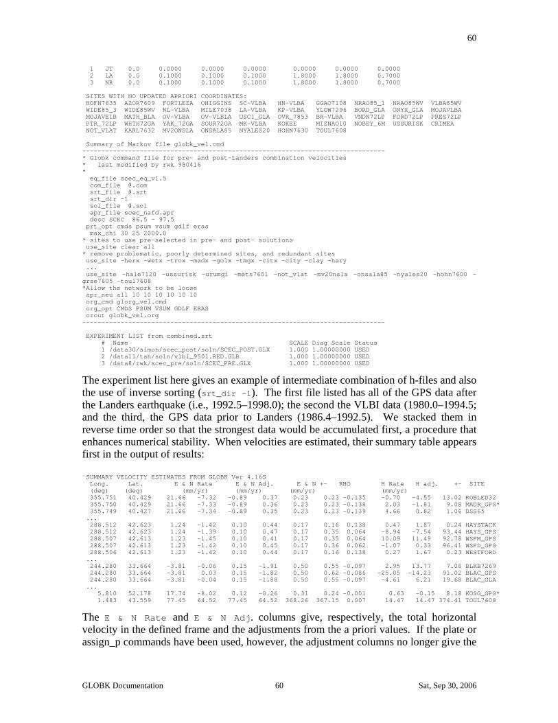
60

1 JT 0.0 0.0000 0.0000 0.0000 0.0000 0.0000 0.0000 2 LA 0.0 0.1000 0.1000 0.1000 1.8000 1.8000 0.7000 3 NR 0.0 0.1000 0.1000 0.1000 1.8000 1.8000 0.7000 SITES WITH NO UPDATED APRIORI COORDINATES: HOFN7635 AZOR7609 FORTLEZA OHIGGINS SC-VLBA HN-VLBA GGAO7108 NRAO85_1 NRAO85WV VLBA85WV WIDE85_3 WIDE85WV NL-VLBA MILE7038 LA-VLBA KP-VLBA YLOW7296 BORD_GLA ONYX_GLA MOJAVLBA MOJAVE1B MATH_BLA OV-VLBA OV-VLBLA USC1_GLA OVR_7853 BR-VLBA VNDN72LP FORD72LP PRES72LP PTR_72LP WHTH72GA YAK_72GA SOUR72GA MK-VLBA KOKEE MIZNAO10 NOBEY_6M USSURISK CRIMEA NOT_VLAT KARL7632 MV2ONSLA ONSALA85 NYALES20 HOHN7630 TOUL7608 Summary of Markov file globk_vel.cmd ------------------------------------------------------------------------------- * Globk command file for pre- and post-Landers combination velocities * last modified by rwk 980416 * eq_file scec_eq_v1.5 com_file @.com srt_file @.srt srt_dir -1 sol_file @.sol apr_file scec_nafd.apr desc SCEC 86.5 - 97.5 prt_opt cmds psum vsum gdlf eras max_chi 30 25 2000.0 * sites to use pre-selected in pre- and post- solutions use_site clear all * remove problematic, poorly determined sites, and redundant sites use_site -herx -wetx -trox -madx -golx -tmgx -citx -city -clay -hary ... use_site -hale7120 -ussurisk -urumqi -mets7601 -not_vlat -mv20nsla -onsala85 -nyales20 -hohn7600 -grse7605 -toul7608 *Allow the network to be loose apr_neu all 10 10 10 10 10 10 org_cmd glorg_vel.cmd org_opt CMDS PSUM VSUM GDLF ERAS orout globk_vel.org ------------------------------------------------------------------------------- EXPERIMENT LIST from combined.srt # Name SCALE Diag Scale Status 1 /data30/simon/scec_post/soln/SCEC_POST.GLX 1.000 1.00000000 USED 2 /data11/tah/soln/vlbi_9501.RED.GLB 1.000 1.00000000 USED 3 /data8/rwk/scec_pre/soln/SCEC_PRE.GLX 1.000 1.00000000 USED

The experiment list here gives an example of intermediate combination of h-files and also the use of inverse sorting (srt_dir -1). The first file listed has all of the GPS data after the Landers earthquake (i.e., 1992.5–1998.0); the second the VLBI data (1980.0–1994.5; and the third, the GPS data prior to Landers (1986.4–1992.5). We stacked them in reverse time order so that the strongest data would be accumulated first, a procedure that enhances numerical stability. When velocities are estimated, their summary table appears first in the output of results: SUMMARY VELOCITY ESTIMATES FROM GLOBK Ver 4.16S Long. Lat. E & N Rate E & N Adj. E & N +- RHO H Rate H adj. +- SITE (deg) (deg) (mm/yr) (mm/yr) (mm/yr) (mm/yr) 355.751 40.429 21.66 -7.32 -0.89 0.37 0.23 0.23 -0.135 -0.70 -4.55 13.02 ROBLED32 355.750 40.429 21.66 -7.33 -0.89 0.36 0.23 0.23 -0.138 2.03 -1.81 9.08 MADR_GPS* 355.749 40.427 21.66 -7.34 -0.89 0.35 0.23 0.23 -0.139 4.66 0.82 1.06 DSS65 ... 288.512 42.623 1.24 -1.42 0.10 0.44 0.17 0.16 0.138 0.47 1.87 0.24 HAYSTACK 288.512 42.623 1.24 -1.39 0.10 0.47 0.17 0.35 0.064 -8.94 -7.54 93.44 HAYS_GPS 288.507 42.613 1.23 -1.45 0.10 0.41 0.17 0.35 0.064 10.09 11.49 92.78 WSFM_GPS 288.507 42.613 1.23 -1.42 0.10 0.45 0.17 0.36 0.062 -1.07 0.33 96.41 WSFD_GPS 288.506 42.613 1.23 -1.42 0.10 0.44 0.17 0.16 0.138 0.27 1.67 0.23 WESTFORD ... 244.280 33.664 -3.81 -0.06 0.15 -1.91 0.50 0.55 -0.097 2.95 13.77 7.06 BLKB7269 244.280 33.664 -3.81 0.03 0.15 -1.82 0.50 0.62 -0.086 -25.05 -14.23 91.02 BLAC_GPS 244.280 33.664 -3.81 -0.04 0.15 -1.88 0.50 0.55 -0.097 -4.61 6.21 19.68 BLAC_GLA ... 5.810 52.178 17.74 -8.02 0.12 -0.26 0.31 0.24 -0.001 0.63 -0.15 8.18 KOSG_GPS* 1.483 43.559 77.45 64.52 77.45 64.52 368.26 367.15 0.007 14.47 14.47 374.41 TOUL7608

The E & N Rate and E & N Adj. columns give, respectively, the total horizontal velocity in the defined frame and the adjustments from the a priori values. If the plate or assign_p commands have been used, however, the adjustment columns no longer give the


61

adjustments with respect to the values (frame) of the apr_file, but rather residuals with respect to the plate defined for that site. SUMMARY POSITION ESTIMATES FROM GLOBK Ver 4.16S Long. Lat. dE adj. dN adj. dE +- dN +- RHO dH adj. dH +- SITE (deg) (deg) (mm) (mm) (mm) (mm) (mm) (mm) 355.751 40.429 -26.9 14.5 13.7 13.5 -0.003 7.6 109.5 ROBLED32 355.750 40.429 1.2 -1.5 1.5 1.3 0.023 7.6 44.7 MADR_GPS* 355.749 40.427 14.4 -11.7 13.5 13.4 0.013 -10.9 14.0 DSS65 ... 288.512 42.623 7.2 -3.7 10.2 10.0 -0.007 -13.3 13.4 HAYSTACK 288.512 42.623 290.2 152.4 34.8 22.1 0.196 -859.2 829.6 HAYS_GPS 288.507 42.613 43.6 11.9 3.8 2.3 0.052 -2.0 17.7 WSFM_GPS 288.507 42.613 100.5 46.8 21.8 15.3 -0.172 -343.2 970.4 WSFD_GPS 288.506 42.613 5.7 -3.7 10.2 10.0 -0.007 -5.4 13.4 WESTFORD ... 244.280 33.664 -2.8 -12.6 1001.6 1001.6 0.000 74.1 1001.1 BLKB7269 244.280 33.664 62.2 -27.8 2.9 2.0 0.023 -81.4 130.6 BLAC_GPS 244.280 33.664 100.6 -43.7 2.7 2.8 -0.052 67.4 98.3 BLAC_GLA ... 5.810 52.178 -1.7 0.8 1.2 0.9 -0.002 20.0 33.6 KOSG_GPS* 1.483 43.559 -681.0 244.6 21.6 21.4 0.014 -14.3 28.9 TOUL7608

The small adjustments (< 0.5 mm/yr) away from the a priori (ITRF96) values for the Westford/Haystack stations, which were not used in stabilization, is a comforting check on the reference frame and the solution as a whole. Note that all of the stations for which horizontal velocities were equated have the same adjustments and estimated values. If this is not true, then most likely you have failed to make the a priori values of velocity the same in the apr_file. In this multiyear solution we have allowed the heights of some of the stations to be stochastic in order to render the estimates of horizontal positions and velocities insensitive to blunders in recording the heights of antennas. This causes the sigmas on height rates to be large (~90 mm/yr in the example). Allowing stochastic heights compromises your ability to detect problems in the solution but does not weaken significantly the estimates of horizontal positions and velocities. It should be avoided if possible but used if necessary.


62

3.6 Error messages globk/glred error messages Several categories of error messages are generated by globk. The first are system errors associated with missing or incorrectly formatted files. These have the form GLOBK/update_glorg_apr: IOSTAT error opening file /data1/sites/itrf96.apr ERROR 1018

and can usually be traced to an incorrect path or filename in the command file. The second type of error results from the inability of the program to decode an entry in the command file; e.g., GLOBK/multiread: IOSTAT error decoding file apr_wob 100 100 10 10 0 0 ERROR -1

This highly generic message generated by multiread can indicate a misspelling of the command, a station mentioned in the command not being present in the solution, or an unexpectedly short list of tokens. In the example, shown the problem is the last of these—the apr_wob command requires 8 arguments and has only 6. In this case, no harm is done since the last two are unused and can be ignored. In some cases, there are traps coded that prevent the multiread message from occurring. For example, if you do not include a priori constraints for all the possible radiation pressure parameters (9) in the apr_svs or mar_svs command, globk recognizes that you might have entered them separately with the apr_rad or mar_rad commands: **WARNING** 11 arguments missing from MAR_SVS command. OK if MAR_RAD used **WARNING** 2 arguments missing from APR_RAD command. OK if APR_SVS used

All of the errors mentioned so far are most likely to occur at the beginning of a run, when globk scans the command file and the input h-files. One other potential problem can also be detected at this stage—a station included in the h-files for which you have no entry in the apr_file: **WARNING** ENDD_GPS not in apr_files

If a station is missing from the apr_file, globk will use as a priori values of the coordinates those on the first h-file, so this message need not cause alarm. However, if you plan to equate adjustments of the coordinates or velocities with those of another station, or use the station in glorg to define the reference frame, then you should make sure that the apr_file has correct and matching entries for the station(s). Once the filtering of the data has started, there are warnings, sometimes accompanied by action, whenever the h-file being read is inconsistent with the Kalman filter estimates up to that point or with the a priori values of the parameters. Before adding the new data, globk first compares the estimated values of the parameters in the h-file with the a priori. If they differ by more than the tolerance set by the second argument of max_chii (see Section 3.1), globk will print a message of the form BAD PREFIT coordinates for site HART_GPS Diffs from apriori -14.911 7.236 -2.139 m


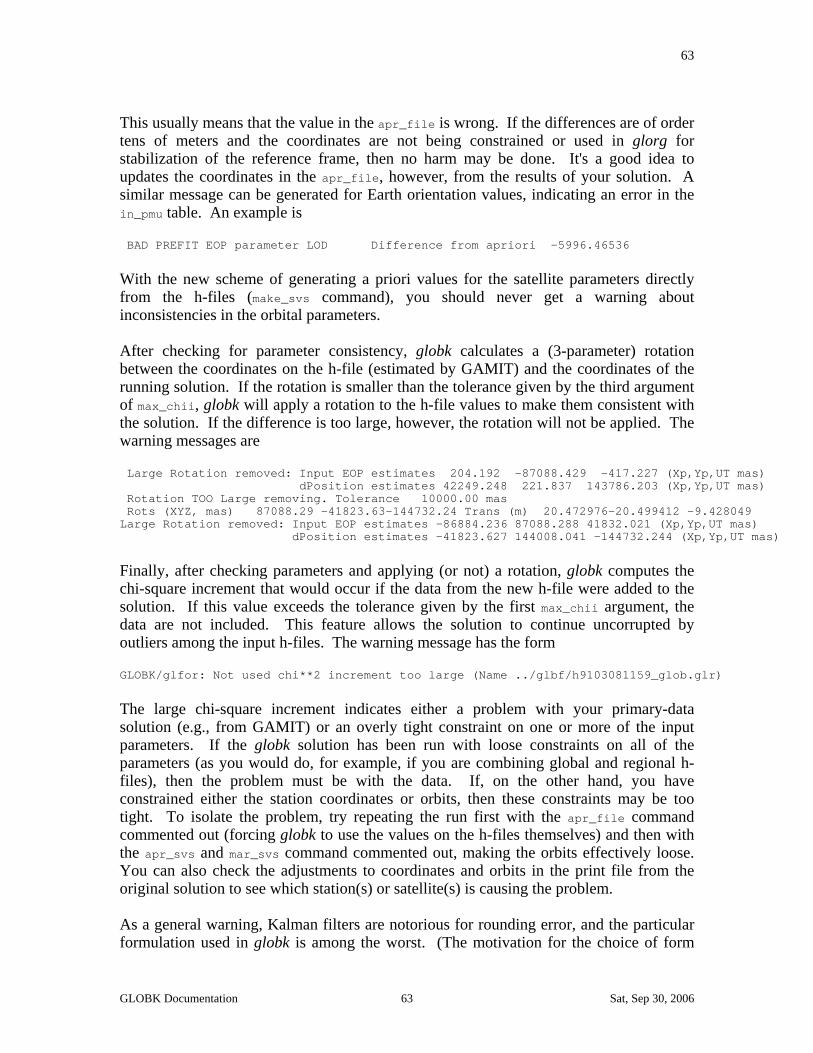
63

This usually means that the value in the apr_file is wrong. If the differences are of order tens of meters and the coordinates are not being constrained or used in glorg for stabilization of the reference frame, then no harm may be done. It's a good idea to updates the coordinates in the apr_file, however, from the results of your solution. A similar message can be generated for Earth orientation values, indicating an error in the in_pmu table. An example is BAD PREFIT EOP parameter LOD Difference from apriori -5996.46536

With the new scheme of generating a priori values for the satellite parameters directly from the h-files (make_svs command), you should never get a warning about inconsistencies in the orbital parameters. After checking for parameter consistency, globk calculates a (3-parameter) rotation between the coordinates on the h-file (estimated by GAMIT) and the coordinates of the running solution. If the rotation is smaller than the tolerance given by the third argument of max_chii, globk will apply a rotation to the h-file values to make them consistent with the solution. If the difference is too large, however, the rotation will not be applied. The warning messages are Large Rotation removed: Input EOP estimates 204.192 -87088.429 -417.227 (Xp,Yp,UT mas) dPosition estimates 42249.248 221.837 143786.203 (Xp,Yp,UT mas) Rotation TOO Large removing. Tolerance 10000.00 mas Rots (XYZ, mas) 87088.29 -41823.63-144732.24 Trans (m) 20.472976-20.499412 -9.428049 Large Rotation removed: Input EOP estimates -86884.236 87088.288 41832.021 (Xp,Yp,UT mas) dPosition estimates -41823.627 144008.041 -144732.244 (Xp,Yp,UT mas)

Finally, after checking parameters and applying (or not) a rotation, globk computes the chi-square increment that would occur if the data from the new h-file were added to the solution. If this value exceeds the tolerance given by the first max_chii argument, the data are not included. This feature allows the solution to continue uncorrupted by outliers among the input h-files. The warning message has the form GLOBK/glfor: Not used chi**2 increment too large (Name ../glbf/h9103081159_glob.glr)

The large chi-square increment indicates either a problem with your primary-data solution (e.g., from GAMIT) or an overly tight constraint on one or more of the input parameters. If the globk solution has been run with loose constraints on all of the parameters (as you would do, for example, if you are combining global and regional h-files), then the problem must be with the data. If, on the other hand, you have constrained either the station coordinates or orbits, then these constraints may be too tight. To isolate the problem, try repeating the run first with the apr_file command commented out (forcing globk to use the values on the h-files themselves) and then with the apr_svs and mar_svs command commented out, making the orbits effectively loose. You can also check the adjustments to coordinates and orbits in the print file from the original solution to see which station(s) or satellite(s) is causing the problem. As a general warning, Kalman filters are notorious for rounding error, and the particular formulation used in globk is among the worst. (The motivation for the choice of form


64

used was driven by the ease of vectoring the computations. On the original computer on which globk was developed this was critical for generating timely solutions.) The effects of rounding error can be greatly minimized by not underconstraining parameters (i.e., do not make the uncertainties of the apriori values of the parameters too large). As discussed in Herring et al. [1990] and Dong et al. [1998], when a priori constraints are applied, the critical quantity is the ratio of the a posteriori to a priori variances of a parameter estimate. The error in adjustment to a parameter value due to the constraint is given approximately by the adjustment times this variance ratio if the correlations among the parameters are small. Thus, if station position is determined to 0.01 m and the a priori constraint was 10 m, then the error in the adjustment due to the constraint is approximately 10-6 times the adjustment. Thus even a kilometer error in the apriori position will only bias the estimate by 1 mm in this case. In practice, the sensitivity is somewhat larger due to correlations, but is probably bounded at n times larger, where n is the number of parameters estimated. The easiest way to assess the effects is just to apply different constraints and see what happens. Files containing a priori values can also be updated if the adjustments are large. glorg error messages Error messages are usually associated with not finding files. If a VREAD -1 (premature end-of-file found) error occurs it usually means that either globk did not complete successfully or that the file containing the solution has been overwritten by another solution. Like globk, the glorg command interpreter will issue a generic warning whenever it does not understand a command, and again this can occur because of a misspelling, missing station, or too few tokens. The most situation is a command file with equates or renames for stations that are not present in the current data set. This situation will be noted by the message ** Error decoding parameter token MONP . Either non-existent station or parameter ** Error decoding parameter token NPOS . Either non-existent station or parameter


65

4. GMT Plotting Utilities Among the shell-scripts of /com are a suite that make use of the public domain GMT plotting package to create various plots from GAMIT and GLOBK output files. The most important of these are sh_plotcrd, which generate time series from glred output, and sh_plotvel, which creates a velocity map from a globk or glorg output. Use of these two scripts is documented briefly in Section 3.4 and more extensively here. These scripts also have online help built into them; by typing the script name you will receive information on what the script does, the input files required and the options that may be selected. sh_plotcrd This script is new with release 10.0 and combines the functions previously performed by ensum (see Section 5.2), sh_histogram , multibase, and sh_baseline, all of which it calls. Basic usage: sh_plotcrd -f <files>

<files> : One or more Glred/globk/glorg print files containing repeated coordinate estimates

Additional options:

-s[pan] (short/long) : Short will set a scale in days and remove only a mean from the time series; long will use years and remove a velocity (but see -o below to override) [default short]

-o[rder] (0 / 1) : Overrides -span for order of polynonial to fit to data

-v[ert] : Overrides -o and -s, forcing no rate estimate for the vertical component

-r[es] : Plot timeseries as residuals [default no]

-e[xpt] name : Experiment name used for naming files and labeling plots; if omitted, the plot files will have generic names related to the program that created them.

-k[ill] sites : One or more sites to remove from plotting.

-b[ase] name : Name of file containing sites to be used; format is a single column, with the 4- or 8-character site name beginning in column 2 [Default: all].

-u[scale] value : Scale uncertainties by this value

-c[ols] (1 or 2) : Number of stations per page [default 2]

Example: sh_plotcrd -f *.org -res -expt emed98


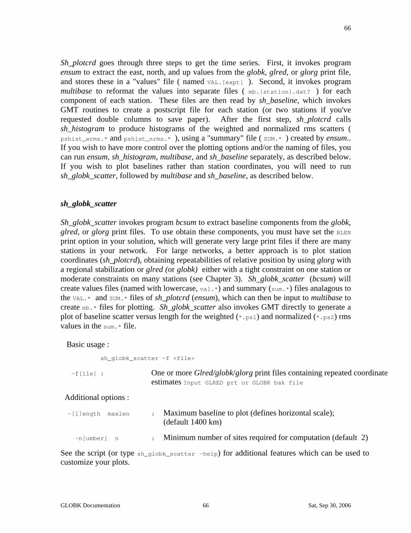
66

Sh_plotcrd goes through three steps to get the time series. First, it invokes program ensum to extract the east, north, and up values from the globk, glred, or glorg print file, and stores these in a "values" file ( named VAL.[expt] ). Second, it invokes program multibase to reformat the values into separate files ( mb.[station].dat? ) for each component of each station. These files are then read by sh_baseline, which invokes GMT routines to create a postscript file for each station (or two stations if you've requested double columns to save paper). After the first step, sh_plotcrd calls sh_histogram to produce histograms of the weighted and normalized rms scatters ( pshist_wrms.* and pshist_nrms.* ), using a "summary" file ( SUM.* ) created by ensum.. If you wish to have more control over the plotting options and/or the naming of files, you can run ensum, sh_histogram, multibase, and sh_baseline separately, as described below. If you wish to plot baselines rather than station coordinates, you will need to run sh_globk_scatter, followed by multibase and sh_baseline, as described below. sh_globk_scatter Sh_globk_scatter invokes program bcsum to extract baseline components from the globk, glred, or glorg print files. To use obtain these components, you must have set the BLEN print option in your solution, which will generate very large print files if there are many stations in your network. For large networks, a better approach is to plot station coordinates (sh_plotcrd), obtaining repeatabilities of relative position by using glorg with a regional stabilization or glred (or globk) either with a tight constraint on one station or moderate constraints on many stations (see Chapter 3). Sh_globk_scatter (bcsum) will create values files (named with lowercase, val.*) and summary (sum.*) files analagous to the VAL.* and SUM.* files of sh_plotcrd (ensum), which can then be input to multibase to create mb.* files for plotting. Sh_globk_scatter also invokes GMT directly to generate a plot of baseline scatter versus length for the weighted (*.ps1) and normalized (*.ps2) rms values in the sum.* file. Basic usage : sh_globk_scatter -f <file>

-f[ile] : One or more Glred/globk/glorg print files containing repeated coordinate estimates Input GLRED prt or GLOBK bak file

Additional options :

-[l]ength maxlen : Maximum baseline to plot (defines horizontal scale); (default 1400 km)

-n[umber] n : Minimum number of sites required for computation (default 2)

See the script (or type sh_globk_scatter -help) for additional features which can be used to customize your plots.


67

multibase

Multibase reads the "values" file created by ensum or bcsum (called by sh_globk_scatter) and creates separate (mb.*) files for each component of each station so that sh_baseline can direct them easily to the GMT plotting scripts. To avoid creating plots for stations you don't want to see (though this is dangerous!) or to keep the number of baseline plots to a reasonable level, you can specify the stations you want using a list, specified in a "sites" file. The stations are simply listed, singly or in pairs (case-independent, with column one blank): SITE1 | plot all combinations with SITE1 SITE2 SITE3 | plot SITE2-SITE3 SITE3 SITE6 | plot SITE3-SITE6 For example, if the sites file is named baselines, and you want to plot the output of sh_baseline_scatter: multibase val.* -s baselines -d

where -d indicates that the time argument is days (-y selects years). The output files are named mb_[SITE].datn, where n is 1, 2, 3, 4 for north, east, up, and length, respectively.

sh_baseline

Sh_baseline reads the mb.* files created by multibase and calls GMT programs to create time-series plots. Basic usage : sh_baseline -f mb*

-f files : Files from multibase to be plotted; all begin with mb_

or -F filename : where filename is a file containing a list of specific mb_ files

The following additional options are available for producing custom plots:

-erase : Erase all psbase files in the directory (default is to overwrite only those that match the names of new ones)

-res : Plot residuals to polynomial fit

-u : Scale factor for uncertainties; default = 1.

-com file Creates length file from bcsum output com-file (component) and gets baseline lengths. If not issued, the value from values-file is passed to the plot.


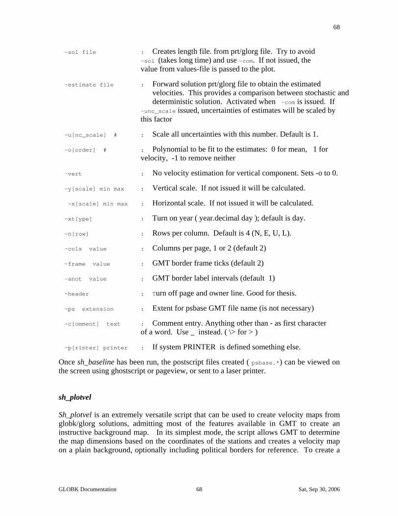
68

-sol file : Creates length file. from prt/glorg file. Try to avoid -sol (takes long time) and use -com. If not issued, the value from values-file is passed to the plot.

-estimate file : Forward solution prt/glorg file to obtain the estimated velocities. This provides a comparison between stochastic and deterministic solution. Activated when -com is issued. If -unc_scale issued, uncertainties of estimates will be scaled by this factor

-u[nc_scale] # : Scale all uncertainties with this number. Default is 1.

-o[order] # : Polynomial to be fit to the estimates: 0 for mean, 1 for velocity, -1 to remove neither

-vert : No velocity estimation for vertical component. Sets -o to 0.

-y[scale] min max : Vertical scale. If not issued it will be calculated.

-x[scale] min max : Horizontal scale. If not issued it will be calculated.

-xt[ype] : Turn on year ( year.decimal day ); default is day.

-n[row] : Rows per column. Default is 4 (N, E, U, L).

-cols value : Columns per page, 1 or 2 (default 2)

-frame value : GMT border frame ticks (default 2)

-anot value : GMT border label intervals (default 1)

-header : Turn off page and owner line. Good for thesis.

-ps extension : Extent for psbase GMT file name (is not necessary)

-c[omment] text : Comment entry. Anything other than - as first character of a word. Use _ instead. ( \> for > )

-p[rinter] printer : If system PRINTER is defined something else.

Once sh_baseline has been run, the postscript files created ( psbase.*) can be viewed on the screen using ghostscript or pageview, or sent to a laser printer. sh_plotvel Sh_plotvel is an extremely versatile script that can be used to create velocity maps from globk/glorg solutions, admitting most of the features available in GMT to create an instructive background map. In its simplest mode, the script allows GMT to determine the map dimensions based on the coordinates of the stations and creates a velocity map on a plain background, optionally including political borders for reference. To create a


69

more eleaborate background, you invoke the sh_plotvel with the name of another script that you have customized for your area of study. Basic usage : sh_plotvel -f <file> -s <site> -ps <filename>

where <file> is the input globk/glorg print file or getrel output <site> is the 4-char station id of reference site for velocities (if omitted, plot absolute velocities); and <filename> is the name given to the output postscript file. The most important options for specifying the velocities are the following: -maxsigma value : Limits stations to those with sigmas less than this value -u value : Scale the uncertainties by this value -i[interval] value : Confidence interval for error ellipses (default 95%) -factor value : Scale the physical size of the velocity arrow by this value -d site1 site2 .. : Remove the sites listed (case insenstive) -D file : Remove the sites listed in the file (single column) Other options, detailed in the script, allow you to site labels, page orientation, error ellipses, and arrow scale. Sh_plotvel will also allow you to superimposed, in different colors, velocity fields from several solutions. To underlay the velocity field with topographic or tectonic features, you can specify inclusion of one or more specific maps (-map <map1> <map2> . , or -maplist <file>) or create for yourself a script that will generate all of the features you need: -mapscript file : Execute the shell script [file] to produce the map Templates for this shell script can be found in /com as sh_map_calif, sh_map_china, sh_map_tien, and sh_map_turk. Within these scripts you prescribe the topography file, whether or not you want color or a gray-scale, and files for tectonic features and labels. Separately, for maximum flexibility, you can specify the range (lat/lon) for the map: -maprange type

which tells sh_plotvel to call script sh_map_elements with the keyword <type> to select a pre-set region (e.g. europe) There are 13 regions already defined, and you can as


70

many of your own as you wish. You can also specify a region explicitly using the GMT range command in the calling sequence; e.g, -R130/170/40/80. Finally, you can also add to your map specialized features such as an Euler pole and small-circle describing relative plate motion; and the epicenter, focal mechanism, and/or slip vector from an earthquake. Examples : sh_plotvel -f turkey.prt -s yigi -mapscript sh_map_turk

sh_plotvel -f tibet_001115b.org -ps 000115b -mapscript sh_map_chinatopo -maprange yunnan2 -maxsigma 10 -u 1 -factor 0.40 -page P -sitefont 8 -arrow_value 20 -D remsite.yunnan


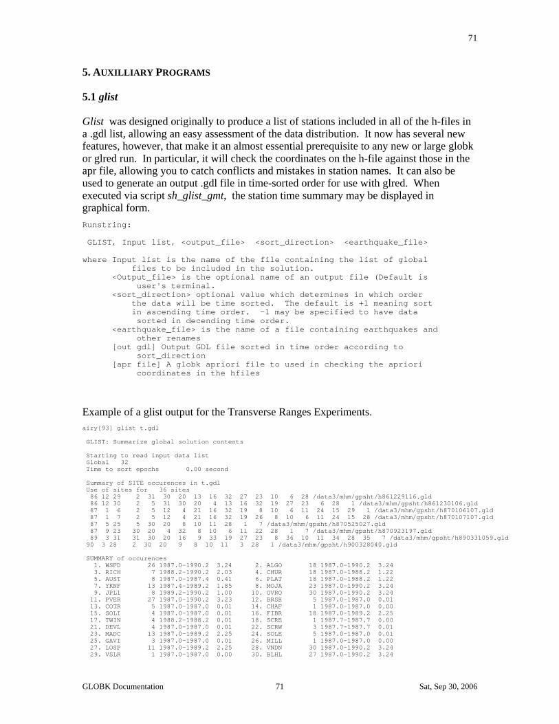
71

5. AUXILLIARY PROGRAMS 5.1 glist Glist was designed originally to produce a list of stations included in all of the h-files in a .gdl list, allowing an easy assessment of the data distribution. It now has several new features, however, that make it an almost essential prerequisite to any new or large globk or glred run. In particular, it will check the coordinates on the h-file against those in the apr file, allowing you to catch conflicts and mistakes in station names. It can also be used to generate an output .gdl file in time-sorted order for use with glred. When executed via script sh_glist_gmt, the station time summary may be displayed in graphical form. Runstring: GLIST, Input list, <output_file> <sort_direction> <earthquake_file> where Input list is the name of the file containing the list of global files to be included in the solution. <Output_file> is the optional name of an output file (Default is user's terminal. <sort_direction> optional value which determines in which order the data will be time sorted. The default is +1 meaning sort in ascending time order. -1 may be specified to have data sorted in decending time order. <earthquake_file> is the name of a file containing earthquakes and other renames [out gdl] Output GDL file sorted in time order according to sort_direction [apr file] A globk apriori file to used in checking the apriori coordinates in the hfiles

Example of a glist output for the Transverse Ranges Experiments. airy[93] glist t.gdl GLIST: Summarize global solution contents Starting to read input data list Global 32 Time to sort epochs 0.00 second Summary of SITE occurences in t.gdl Use of sites for 36 sites 86 12 29 2 31 30 20 13 16 32 27 23 10 6 28 /data3/mhm/gpsht/h861229116.gld 86 12 30 2 5 31 30 20 4 13 16 32 19 27 23 6 28 1 /data3/mhm/gpsht/h861230106.gld 87 1 6 2 5 12 4 21 16 32 19 8 10 6 11 24 15 29 1 /data3/mhm/gpsht/h870106107.gld 87 1 7 2 5 12 4 21 16 32 19 26 8 10 6 11 24 15 28 /data3/mhm/gpsht/h870107107.gld 87 5 25 5 30 20 8 10 11 28 1 7 /data3/mhm/gpsht/h870525027.gld 87 9 23 30 20 4 32 8 10 6 11 22 28 1 7 /data3/mhm/gpsht/h870923197.gld 89 3 31 31 30 20 16 9 33 19 27 23 8 36 10 11 34 28 35 7 /data3/mhm/gpsht/h890331059.gld 90 3 28 2 30 20 9 8 10 11 3 28 1 /data3/mhm/gpsht/h900328040.gld SUMMARY of occurences 1. WSFD 26 1987.0-1990.2 3.24 2. ALGO 18 1987.0-1990.2 3.24 3. RICH 7 1988.2-1990.2 2.03 4. CHUR 18 1987.0-1988.2 1.22 5. AUST 8 1987.0-1987.4 0.41 6. PLAT 18 1987.0-1988.2 1.22 7. YKNF 13 1987.4-1989.2 1.85 8. MOJA 23 1987.0-1990.2 3.24 9. JPL1 8 1989.2-1990.2 1.00 10. OVRO 30 1987.0-1990.2 3.24 11. PVER 27 1987.0-1990.2 3.23 12. BRSH 5 1987.0-1987.0 0.01 13. COTR 5 1987.0-1987.0 0.01 14. CHAF 1 1987.0-1987.0 0.00 15. SOLI 4 1987.0-1987.0 0.01 16. FIBR 18 1987.0-1989.2 2.25 17. TWIN 4 1988.2-1988.2 0.01 18. SCRE 1 1987.7-1987.7 0.00 21. DEVL 4 1987.0-1987.0 0.01 22. SCRW 3 1987.7-1987.7 0.01 23. MADC 13 1987.0-1989.2 2.25 24. SOLE 5 1987.0-1987.0 0.01 25. GAVI 3 1987.0-1987.0 0.01 26. MILL 1 1987.0-1987.0 0.00 27. LOSP 11 1987.0-1989.2 2.25 28. VNDN 30 1987.0-1990.2 3.24 29. VSLR 1 1987.0-1987.0 0.00 30. BLHL 27 1987.0-1990.2 3.24


72

31. BLAN 13 1987.0-1989.2 2.25 32. FTOR 19 1987.0-1988.2 1.22 33. KOKE 4 1989.2-1989.2 0.01 34. TROM 7 1988.2-1989.2 1.04 35. WETT 4 1989.2-1989.2 0.01 36. ONSA 4 1989.2-1989.2 0.01

The error mesages associated with glist are usually file related. Warnings about the apriori values not matching will also be printed when this program is run. 5.2 glsave This program creates a combined binary h-file from the com_file output of a globk run. It provides an alternative to the out_glb command in globk. glsave <com file> [out global name] [description]

where <com file> is the globk common file name (given in the com_file command). [out global name] is an optional output file name. [description] is an optional description for the solution. If there are blanks the description must be enclosed in single quotes (e.g., 'Week 819 run') 5.3 xysum,blsum, bcsum, ensum, enfit These five programs provide a convenient means for extracting coordinate and baseline information from the print files for globk (usually produced by glred runs) and from back solution output files. (See also extract and exbrk for more general extraction software, and multiplot and plot for display software). The program xysum is a utility for getting or updating coordinate values for the .apr file and and the time-distribution of the stations; bcsum, blsum, and ensum generate files for plotting; enfit allows you to estimate functions describing post-seismic behavior and plot the residuals. Specifically: xysum — extracts and averages the cartesian estimates of station coordinates and

velocities, producing an apr file, a values file for plotting, and a summary file giving the time distribution of each station in the solution.

blsum — extracts baselines lengths only and produces a summary file with baselines, wrms scatters about the means, rates of changes and wrms scatters about the rates; and a values file which contains all baselines length determinations (sorted by baseline). This latter file may be used in multiplot to produce plots of the time evolutions of all baseline lengths.

bcsum — extracts baselines and the north, east and up components of the baselines and produces a summary file, similar to blsum, for each baseline with four entries per baselines, one each for baseline length, north component, east component, and up component; and values file which contains the time evolution of baseline lengths and the baseline components. This file may be used as input to multiplot.-

ensum — extracts the North, East and Up components of station positions and produces a summary file and values file similar to blsum. The values file can be input to multiplot and all components will be plotted.


73

enfit— extracts the North, East, and Up component of station positions and performs a fit to the time series for each station, allowing estimation of an offset, rate, and one or more exponential and periodic functions. This program is useful for error analysis and also for studying post-seismic relaxation.

For these programs to be used, output options with bit 1 set (i.e, 2 decimal) must be used during the globk runs. NOTE: The summary files and values files are overwritten by these programs if they already exist. The runstrings for each of these programs is shown below from on-line help files. XYSUM: Generate globk apriori, summary, and a file containing all site XYZ values sorted by site and possibly time. Runstring: xysum <options> <apriori_file> <summary_file> <values_file> <Input solution files> where <options> There are two options that may be passed: (1) controls the sorting and limits on the number of values needed for an output to be made. If option contains a numerical value, then this gives the minimum number of estimates need to produce an output. If this numerical value is negative then the baseline entries will be time sorted before being output to the values file. (The default value is 0 i.e. all entries are output to summary file) <apriori_file> is the name of a globk style apriori file. <summary_file> is the name of the summary file (one line per site and component) <values_file> is the name of file where all the individual site components are written sorted by site and component, and optionally by time. <Input solution files> is a list of input files. These may be generated by globk, glbak, solvk or may be previously obtained values files with the line: VALUES_FILE as the first line of the file. BLSUM: Generate summary and a file containing all the baseline length values sorted by baseline and possibly time. Runstring: blsum <option> <summary_file> <values_file> <Input solution files.> where <option> controls the sorting and limits on the number of values needed for an output to be made. If option contains a numerical value, then this gives the minimum number of estimates need to produce an output. If this numerical value is negative then the baseline entries will be time sorted before being output to the values file. (The default value is 0 i.e. all entries are output to summary file) <summary_file> is the name of the summary file (one line per baseline) <values_file> is the name of file where all the individual baseline lengths are written, sorted by baseline and optionally


74

by time. <Input solution files> is a list of input files. These may be generated by globk, glbak, solvk or may be previously obtained values files with the line: VALUES_FILE as the first line of the file.

The help file for ensum is similar to that for blsum, and will not be given. Bcsum has an extra output file: BCSUM: Generate summary and a file containing all the baseline length values sorted by baseline and possibly time. Runstring: % bcsum <option> <summary_file> <values_file> <component summary> \ <Input solution files.> where <option>, <summary_file>, <values_file>, and <input solution files> are the same as for blsum, and <component summary> is the file containing the summaries for length (L), North (N), East (E) and height (U).

ENFIT: Generate multiparameter fits to time series data generated with globk/glred or from values files produced by ensum Runstring: enfit <option> <-f cmd_file> <summary_file> <values_file> <Input solution files> where <option> has the same meaning as in ensum. A positive numeric value sets the minimum number of measurements needed for a time series to be included. <-f cmd_file> specifies name of command file used to set the parameters to be estimated <summary_file> is summary output file <values_file> is list of input values, residuals and model values from parameter estimates <Input solution files> are globk/glred output files or values files from ensum (name must start with va). The cmd_file contains the commands for the parameter estimates. Exponential function -------------------- EXP <date> <tau> <apriori sigma> [tau sigma] where <date> is yy mm dd hh min for start of exponential, <tau> is the decay time in days <apriori sigma> is apriori contraint to apply to estimate in mm. This command may be issued multiple times to generate results for multiple decay times. [tau sigma] is an optional apriori standard deviation for the time constant. If this argument is included, the time constant will be estimated in a iterative solution. Periodic function ----------------- PER <Period> <apriori sigma> where <Period> is the period in days. The terms have


75

zero time at 2000/01/01 <apriori sigma> is apriori contraint to apply to estimate in mm. This command may be issued multiple times to generate results for multiple periodic terms. Output at specific times ------------------------ OUT <name> <times....> where <name> is name of output file. If the form xx@ is used then the @ is replaced by the coresponding characters from the summary file name. <times....> is a list of days after the epoch of first exponential function to output values. Values can be specfied in form <nn>x<dd> where <nn> is a number of values to output and <dd> is a spacing in days, e.g., 10x100.0 would output values100,200,300...1000 days after the epoch of the first


76

5.4 extract, exbrk Extract and exbrk are general utility programs for extracting information which have some type of repeating structure. They allow information to be obtained from multiple lines in the input and then output on a single line. The two programs are the same except that exbrk will output a status report if any key on your terminal is touched while it is running. In response to this status, you have the option of continuing if everything looks good or aborting the run so that the input control file to extract can be modified. Since extract/exbrk can extract a number of different types of information for each run, you also have the option of skipping to next classs of information to be extracted. These features are very useful when new extract commands file are being developed. They quickly let you see if the commands are working OK, and which lines the program is having trouble finding. Because of this key press sensitity, exbrk cannot be run in background (the program will immediately stop in state waiting for input from your terminal). Even when run in foreground, the feature also poses a problem if the program is executed under script control, since any key pressed at any time during the script execution will cause the status to be printed and the program to wait for response when exbrk is executed. For these reasons, it is recommened that exbrk be used to check the extract command files, and then when you want to use these commands in general processing that extract be used. EXTRACT : Program to extract information from ASCII files Runstring: CI> EXTRACT <command file> [input file] [output file] where <command file> is the name of a file or LU with commands for extract. (See below) [Input file] is an optional name of a file to be decoded. If not given the runstring then name should be given in the command file (see INPUT command) [Output file] is an optional name for the output file. If not given here or in the command file (See OUTPUT command) then LU 1 will be the output device. EXTRACT Commands ---------------- (Note: all commands may be truncated to minimum unique length, and all commands must be preceeded by at least one blank) END -- Tells program to stop reading the command file (EOF has the same effect) INPUT -- Name of the input file. Must be given here or in the runstring. Usage: INPUT my_input_file.txt OUTPUT -- Name of the output file. Defaults to users terminal. Multiple input files may be read for output to the same output file by giving new INPUT commands betweem RUN commands (see below) without re-giving the OUTPUT command. DESCRIPT-- Allows the specification of the header record describing each each of the fields extracted. Note: the description is enclosed in double quotes ("). Usage: DESCRIPT <field #> "<description>" or where field # is the number of the field to which the description applies. (See field command below) TITLE -- Allows a title to be given to the output file. This line will appear as the first line in the output file. Usage: TITLE "<title>" OR TITLE <nn> where <title> is the string to be output and must be encloded in double quotes. <nn> is an alternive form and line NN of the input file will be used as the title. NOTE: No field information will extract until after the <nn> line of the input file is read. FIELD -- Tells the program about the information to be extracted from the data file. This is a complex command which gives the user a great deal of flexibility in the information extracted.


77

The format of the command is: FIELD # "<descriptor>" #_args type {Format 0/1 "(format)" or {Readline 0/1 <entries> OR FIELD # CLEAR. where: # is the field number. EXTRACT allows the user to specify upto to 10 fields of information to be extracted. There three types of field (See type below also). CHaracter -- only one string per field (upto 64 characters long) Integer*2 -- Upto 32 integer values per field Real*8 -- Upto 8 real*8 number per field. If these numbers of arguments are not large enough then you can extract the information using a number of fields. <descriptor> is an Ascii string which tells extract the EXACT string which must be found in the input file for it to extract the field data from the rest of the string. #_args is the number of arguments in the field to be extracted (see above for limits) type is the type of field. Type may CH for charater, I2 for integer*2, R8 for real*8. (see restrictions on number of arguments given above). The next string may be either: FORMAT to extract the field data using a FTN77 format statement OR READLINE to extract the field data using free format reads Indepenent of the use of Format or Readline, the next argument 0/1 tells extract whether to get the data from the line imediately following the <descriptor> (option 0), or from the start of the line (option 1). When FORMAT is used the 0/1 is followed by the FTN77 format enclosed in double quotes(don't forget the parentheses around the format, When READLINE is used the 0/1 is followed by #_args values which tell EXTRACT which values for the rest of the line should be used. For expample, if your input line looked like: string 120 baseline 200 10 20 0.110 -- Line 1 2 3 4 5 6 7 -- Item numbers then Items 2 4 5 6 and 7 could be read with R8 or I2 (although item 7 would be zero in I2 format). Any of the items 1-7 could be extracted with a character field (although only one item per field.) [If you wanted a character field with the complete line above, then FORMAT would be the only choice. The other option for the field command is CLEAR which will clear the information about the field. Thus this field will no longer be searched for. BEGIN -- Allows the specfication of strings which must be found before a field will be searched for. Usage: BEGIN # number "<string>" where # is the field number to which the begin applies, number is the number of the begin when more than one string must be found. Number is currently limited to two ie. upto two different string can be specified before the field will be extracted. <string> is the EXACT string to be found (enclosed in double quotes. FINISH -- Allows the specifiction of a string which will cause EXTRACT to to stop seaching for a field and to reset the field as being no yet found. Usage: FINISH # "<string>" where # is the field number and <string> is the EXTRACT string to be found( again enclosed in double quoutes. NOTE: Since extract will only output the field data when all fields have been found, the FINISH strings should all appear after all of the FIELD strings in the input file. NORESET -- Allows the specifications of fields which should not have there found status set False after the field data has been output. Useage: NORESET nn nn nn OR NORESET CLEAR where nn are a list of field numbers to not be reset, the CLEAR option will clear all previously set NORESET values. OUTFORM -- Allows the user to specify the output format for each of the fields. Usage: OUTFORM # "(format)" where # is the field field number, and (format) is the FTN77 format to be used. (Enclosed in double quotes.) NOTE: when strings are output trailing


78

blanks will be deleted during the output. RUN -- Tells extract to process the input file with the current field information. THIS COMMAND MUST BE GIVEN OR ELSE EXTRACT WILL DO NOTHING. NOTES: ------ EXTRACT defaults to field 1 searching for EXPERIMENT DATE: with the date read with a format. This is used for extracting information from the SOLVK and GLBAK solution files. This field is also set for NORESET so that the same exeriment date can be used for many items from a SOLVK solution. EXTRACT will resond to a break issued from a system prompt, by summaring its progress so far i.e., number of lines read and written, and current status of fields and begins being found. (NOTE: usually a field will appear as not found, since it is reset after each output). The user then has the option of Aborting (stopping EXTRACT immediately), of stopping the processing of the current run, or continuing with the current processing. EXAMPLE: The following extract command file will extract the statistics . form a SOLVK solution file. NOTE: Any character in column one will . cause the line to be treated as a comment . Line below is a comment but could be used to get pre-fit statistics . instead of postfit. If we wanted to we could do both together. .field 2 "pre-fit Chi**2/f is" 1 CH readline 0 1 . Note we are extracting two things from the same line. field 2 "All baselines" 1 CH format 0 "(7x,a20)" field 3 "All baselines" 1 CH format 0 "(34x,a20)" . This will get total number of data (see SOLVK output) field 4 "From" 1 R8 readline 0 1 field 5 "DATA file" 1 CH Readline 0 1 outform 2 "(a20)" outform 3 "(2x,a20)" outform 4 "(1x,I5)" outform 5 "(2x,a12)" run ! NOTE COMMAND NEEDED . There are a number of other examples in the /SOLUTIONS/ directory . which contain extract command files. (All have .EXT extensions)

In response to pressing a key exbrk will respond as follows. (The text below shows the program run line as well.) In this example, the program was allowed to continue after the first break, and then aborted. chandler[52] exbrk UT1.ext /data5/tah/soln/sk901120.prt UT1_901120.dat EXTRACT STATUS: Line 422 in input, Line 2 in output Field 1 Label EXPERIMENT date : Field found T Starts found Field 2 Label UT1 Diurnal Cosine Field found F Starts found Field 3 Label UT1 Diurnal Sine Field found F Starts found Field 4 Label UT1 SemiDiurnal Cosi Field found F Starts found Field 5 Label UT1 SemiDiurnal Sine Field found F Starts found Field 6 Label Solution Field found T Starts found T Field 7 Label DATA file Field found T Starts found Last line written to output 1985 1 4 6 3 -1.120 41.303 0.267 41.714 -0.557 75.160 -0.734 75.160 1 ../ko_eor/k850103i.kal Option: A-Abort EXTRACT, S-stop this search, C-continue ? c EXTRACT STATUS: Line 764 in input, Line 3 in output Field 1 Label EXPERIMENT date : Field found T Starts found Field 2 Label UT1 Diurnal Cosine Field found F Starts found Field 3 Label UT1 Diurnal Sine Field found F Starts found Field 4 Label UT1 SemiDiurnal Cosi Field found F Starts found Field 5 Label UT1 SemiDiurnal Sine Field found F Starts found Field 6 Label Solution Field found T Starts found T Field 7 Label DATA file Field found T Starts found Last line written to output 1985 1 9 5 57 -0.693 41.299 0.018 41.712 -0.525 75.160 -0.443 75.160 1 ../ko_eor/k850108i.kal Option: A-Abort EXTRACT, S-stop this search, C-continue ? a STOP: EXTRACT Terminated : At break chandler[53]

5.5 getrel


79

Getrel is a program which allows the relative velocities of stations to be extacted from a globk solution in such a way that they can be plotted using plot with error ellipses. To use getrel, velocities must be be estimated and glorg run with the output options brat:svel set . This output will produce the summary of station velocities and the velocities of the baseline components. Since the baseline components are output for the western directed baselines only, getrel will reverse the direction on the baseline to make the velocity components relative to station specified in the input runstring to to the program. The instructions for using getrel are given in the online help file. Any example of a plot control file to plot the output from getrel is also given below. GETREL: Program to extract station specific relative velocites This program will get the relative velocities of a group of stations and print the results in a format comparable to the standard NE velocity output from GLOBK. Runstring is: % getrel <site> <input file> <max_sigma> where <site> is the name of the station the velocities are to be given relative to. <input file> in the name of the file output from GLOUT or GLORG. Output options brat:svel should be set <max_sigma> is the size of the maximum sigma to be output. (Default is to output all)

5.6 swaph, hfupd, htoh These three programs alter existing h-files to achieve binary byte-order compatibility or to change incorrect information. The first program, swaph, is used to change from BIG-ENDIAN (HP, Sun) binary to little-endian (PC, DEC) binary: swaph < h-files >

where < h-files > is the names of the files to be changed, with standard Unix wild-cards allowed (i.e., swaph h* ). The program will sense the type of machine you are on and change the bytes only if necessary to be compatible with that machine's architecture. The files are rewritten in place, and the version number of the h-file, stored internally, is changed to indicate the te bytes have been swapped. Program hfupd compares the entries on an h-file with those on a current GAMIT station.info file or a SINEX file and changes all that do not agree. Because of the high cost in storage and cpu to read and write a large number of h-files, hfupd is designed to make the changes in place (taking advantage of a direct-access read/write), overwriting the old h-file. Since the results of hfupd are non easily reversible, you can/should run it initially without the -u (update) option to be sure that you know what changes will be made. . hfupd <options> <list of hfile names> Options: -s <sinex file/station.info> Use the named sinex file or station.info file to check antenna type and eccentricities. The program reads the complete station.info file so expect the program to stop for any errors in station.info.


80

(A Gamit standard routine is used which generates a fatal error, so you will need to find the problems one-at-a-time). When station.info is used, antmod.dat and rcvant.dat must be available, either in the local directory or $HOME/gs/tables. -e <edit file> Edit the site/satellites based on list contained in <edit file>. This option is the equivalent to use_site -<name> is globk. Sites may be restored later provided the a new hfile has not been generated with the edited h-file. The renames are applied before checking the headers. So when station.info is used, sites can be renames to end in _GPS which are the only ones checked when station.infois used. -r Report the contents of the sinex/station.info file given with the -s option -u Update the hfile. This option must be given for the hfile to be updated. The hfile is re-written in place so the changes are permanent. -d Report only the differences between the hfile and sinex/station.info file headers. -p <hf/pmu file> Apply the pole-tide correction. The file will be marked as having the pole tide applied and so it will not be reapplied in globk. If -p hf used then the hfile values for pole position will used. The reccommended form is -p <pmu file name> which will used pmu file values for pole positions. -h [list:] Update headers only and not the solution vector. The [list:] includes a : separated list of quanities to be updated. ant -- Antenna information ptd -- Mark file as having pole tide applied without actually applying the pole tide. These features are useful for correcting inconsistent information, especially from sinex files (rather than ascii hfiles which contain information consistent with the solution). With the pole tide, the sinex file has no information to indicate that it has been applied. Analysis center reports must be relied upon for this information. EDIT FILE options: The following entries may be included in the edit file. All entries start with at least one blank character. All options are optional except the site name (and rename site for rename command). UNWEIGHT <NAME> <HF code> <Epoch range> RESTORE <NAME> <HF code> <Epoch range> RENAME <OLD NAME> <NEW NAME> <HF code> <Epoch range> where <NAME> is the full name of the site <HF code> is a character string that must appear in the hfile name (16 characters max, optional, must not be all numeric) <Epoch range> specified as start yr, mth, day, hr, min and end yr, mth, day, hr, min <OLD NAME> is the old name of a site <NEW NAME) is the new name of a site The edit file does not allow positions to be changed directly. Such changes should be made through the appropriate sinex header antenna information.


81

Program htot changes the names of the stations in a GAMIT ASCII h-file. This program is used to allow the station codes to be changed to those used in a particular local analysis. Htoh is rarely used now that the rename command is available in globk. HTOH: Change station names in hfiles This program will read an h-file and change the names of the stations listed in the key file to the new name given there. The history entries will be appended below the GAMIT Datum line in the file. The runstring for the program is % htoh <key file> <list of hfiles ....> where <key file> is the list of stations names to change with optional comment lines in the file. (The comment lines denoted by a non-blank character in column 1 are ignored.) The format of the key file is: OLDN NEWN with OLDN the old name of the station and NEWN the new name. The Names must 4 characters long and spacing is not critical except column 1 must be blank. and <list of hfiles ....> is a list of hfiles to change. The new h-files are written out with the same name as the old ones. The old hfiles be deleted as each new hfile is sucessfully written. While the new files are being generated the original hfile is named <name>.org. Any pre-existing .org file will be overwritten. The list of hfiles can use UNIX wild cards.

5.7 glbtog This program will read a globk print file or bak file and generate a series of g-files that can be used in GAMIT processing. glbtog: Make g-files from GLOBK/GLBAK output -------------------------------------------- PROGRAM GLBTOG: make G-files from Globk output This program will read either globk output files or glbak output files and generate GAMIT G-files for all the epheremis elements that it finds. The runstring is: % glbtog <globk/glbak file> [4-5 character code] ['Comment line'] where <globk/glbak file> is the name of the globk output or glbak file and [4-5 character code] is an optional 4 or 5 character code to be used in the G-file name. If four characters are given the fifth will be the last digit of the year. If no name is given then 'glbkY' will be used where Y is the last digit of the year. ['Comment line'] is an optinal comment line. If the comment includes blanks then it must be enclosed in single quotes (') ** WARNINGS **


82

+ This program will overwrite existing gfiles with the same name as those generated by the program + If multiple G-files will be produced then an end numerical value will be added to the name. + Since GLOBK/GLBAK only output orbital elements for those SV's with data, the gfile produced here may need to be edited to add those satellites in the xfile headers for which there is no data. + Be careful with multiday, stochastic orbits. When these g-files are used again in GAMIT and globk used to processes the output files, globk will not know that the orbits are not fully dynamic. + This program produces warnings if the radiation parameters deviations are greater than 30%. It is not recommended for these orbits to be re-integrated. + In addition to the IC values, the sigmas from the Globk solution are also added to the file. The units of the sigmas are the same as globk units (meters, mm/sec and unitless). The sigma units are different to the orbital element units. The runstring is: % glbtog <globk/glbak file> [4-5 character code] ['Comment line']

5.8 glbtosnx This program will read globk ver 1.0 and greater binary h-files and write out IGS standard Solution INdependent EXchange (SINEX) files. The runstring is glbtosnx <dir> <comments file> <input binary hfile> <output file name> where <dir> is the directory to write files to (use . for the current directory. <comments files> is a file containing comments for SINEX file. If no name is given (i.e., ' ' is used) then a default name head.snx will be tried. If the file is not available no comments will be written to the sinex file. (The file will still be valid). <input binary hfile> is the input binary file. <output file name> is the output file name or root. If nothing is specifed then the name will be <owner><gps week><gps day of week>.snx if one character is given <gps day of week> is replaced with that character. In the full name: #### will be replaced by <gps week><gps day of week> and ### will be replaced by <gps week>.

The format of the comments file is similar to the SINEX itself. An example is given in head.snx in the $(HELP_DIR) directory. We have augmented the current SINEX format by entries to allow the DOMES numbers to be defined. These are also given in head.snx.


83

5.9 corcom, cvframe, velrot There are three programs available to compare coordinates or velocities estimated in different reference frames. Corcom uses the cartesian coordinates and velocities in an apr file transforms them between pairs of frames related by an Euler vector. Transformations built into the program include those relating the ITRF or NUVEL-1A no-net-rotation frame to frames attached to each of the major plates, using the NUVEL-1A Euler poles and rates. Cvframe does the same thing but uses the velocity summary (vel file) in east, north, and up from a globk or glorg print file. Velrot reads a pair of vel files and estimates transformation parameters relating them. Hence it can be used to bring into a single reference frame velocity solutions from different analyses, even those provided by outside groups. In all three programs, it is possible to exclude or downweight height in performing the transformation. CORCOM: Program for the comparison of station coordinates estimated by difference systems. The runstring of the program is: corcom <sys1> <frame1> <sys2> <frame2> <outname> <out_frame> \ <ties> <fundamental sites> <height wght> <scale> where <sys 1> is the name of the file containing the stations and their coordinates and velocity in system 1 <frame 1> is the frame for this first system. (See frames below.) <sys 2> is the second (comparison) system. Sys 1 will be rotated and translated into this frame. Differences will be given between sys1 and sys2 in this frame. <frame 2> is the frame for this second system. Same choices as above. Default NAFD_1990.0 where the end characters are the epoch of the frame to be used. (Only used for the out_frame) <outname> is name of file for output of frame (overwritten) <out_frame> is the frame for the output field (as above) <ties> if the file containing station ties. The file is interpretted as using the second station name in the tie to generate the position of the first tie. The ties are only applied to the stations in sys 1. (May be neglected in runstring---no ties will be used) <fundamental sites> names of stations to be used for rotation and translation (names after ties have been applied) If not given then all stations are used. ALL may be given as name and all common stations will be used. A '-' in front of name will stop it being used. <height wght> Weight to be given to heights in the transformation determination. If 1 then equal weight given. If 0 then no weight is given (default is not to used heights) <scale> indicates that scale should be estimated (Y will cause sacle to be estimated, unless height weight is zero, in which case scale can not be estimated. is zero, in which case scale can not be estimated. The following frame names are supported: PCFC, COCO, NAZC, CARB, SAFD, ANTA, INDI, AUST, AFRC, ARAB, EURA, NAFD, JUAN, PHIL, NUV-NNR, AM-02, ITRF93, ITRF94. E.g. NAFD_1993.4 for the output frame would North America fixed with coordinates aligned at 1993.4. The rates are calculated using NUVEL-1A unless a ":0" is added to the name (e.g. NAFD:0), in which case NUVEL-1 will be used. CVFRAME: Program to change velocity reference frame in .vel files


84

The runstring of the program is cvframe <in vel> <out vel> <inframe> <outframe> where <in vel> is the input velocity field file <out vel> is the output velocity field generated by this program <inframe> is the reference frame for the input field <outframe> is the reference frame for the output field or an Euler pole vector passed as three values for wx, wy, wz (deg/Myr units). Values must be enclosed in ' '. The Frame names follow the PLATE program convention. VELROT: Program to combine velocity fields Usage: velrot <sys1> <frame1> <sys2> <frame2> <outname> <out_frame> \ <link file> <height weight> <param_opt> where <sys1> Globk velocity file for System 1 <frame1> Reference frame for system 1. See corcom help for list of available frames. <sys2> Globk velocity file for System 2. System 1 will transformed into System 2 (reference system) <frame2> Reference frame for System 2 <outname> Output file name containing the combined velocity field <out_frame> Reference frame for output system <link file> File containing options for sites to be used in linking the velocity fields. If the option is not given, all sites with the same name will be used. <height weight> Weight to be given to the height velocity <param_opt> Options for parameters to be estimated to transform the two fields. They are: T - Translation R - Rotation S - Scale L - Local 2-parameter transformation (should only be by itself) The option is specified as single string. The default is TR) Only the first two arguments are required. Program operation and output ---------------------------- The two input systems are transformed to the output frame and, based on the options given in the link file, "common" stations are used to transform System 1 to best match System 2. The options in the link file are (all lines start with at least one blank.: eq_dist <distance (m)> Finds all sites separated by less than the distance given and uses these sites to align the frames. Sites can occur multiple times in these lists. Normally, this command is given first. cp_dist <distance (m)> For comparison/evaluation purposes, can be set so that all sites separated by less than this distance are marked in the output with an * at the end of the site name. If option is not used, eq_dist is used. +-site_name +-site_name Lines of this type allow specific sites to be included or excluded from the list of sites used in the


85

alignment. Preceding a site name with a - will exclude it from the list, a + or no symbol will cause it be included. If only one site name appears, then the second site name is assumed to be the same. Nominally, the first name applies to system 1 sites, and the second name to system 2. The comparison of names is done with casefolded strings. Example link_file: * Set the nominal separation of sites to be 1 km. eq_dist 1000 * * Exclude list * Any occurrence of g005_gps in the alignment sites from * system 1 will be removed -g005_gps * Any occurrence of c100_bas in System 1 alignment sites, and * newp_gps in System 2 aligment sites are removed -c100_bas -newp_gps * Include list * If jplm_gps occurs in both systems include in the alignment * sites (note: in this file this will result in the site being * used twice) jplm_gps * If e200_bas and egan_gps occur in both files, add to the * aligment list. (+ at beginning of name is not needed) +e200_bas +egan_gps Height_weight - The weight of the height velocities to be used in transforming between the systems can be specified with this argument. Default is height_weight = 1 (weight is applied to velocity covariance matrix based on the sigmas in the velocity files. Setting the weight to 0 will cause the height velocities not to be used at all in the alignment. Param_opt - Options for the parameters to be estimated in transforming between the systems. If this argument is not given the default TR parameters are used. To have no parameters estimated, use a values other then TRSL, e.g., X. Output ------ The output file first contains the statistics of the alignment of the systems and the residuals of the sites used in the alignment. These residual lines start with the letter A (for grepping).and contain the residual velocities at the alignment sites (dN, dE, dU), the combined sigma of the pairs of velocity estimates in the residuals (sN, sE, sU), and the contributions of the transformations uncertainties at these sites (sTN, sTE, sTU). The second block of the output contains the velocities from System 1 given in the System 2 frame. The sigmas given here include the contribution from the uncertainty in the trans-formation parameters. The final block gives the velocities of the sites in System 2. If a site name here matches exactly a name from System 1, 3. the entry has a - symbol in the first column (thus is 4. made a comment). In both outputs, sites in different systems which are separated by less than cp_dist will be marked with a * for System 1 and a '+' for System 2 at the end of the site name. To see which sites will be used for alignment, the following sequence can be used: comb.list contains cp_dist 10000 Then % velrot sys1,vel nafd sys2.vel nuv-nnr sysout.vel pcfc comb.list


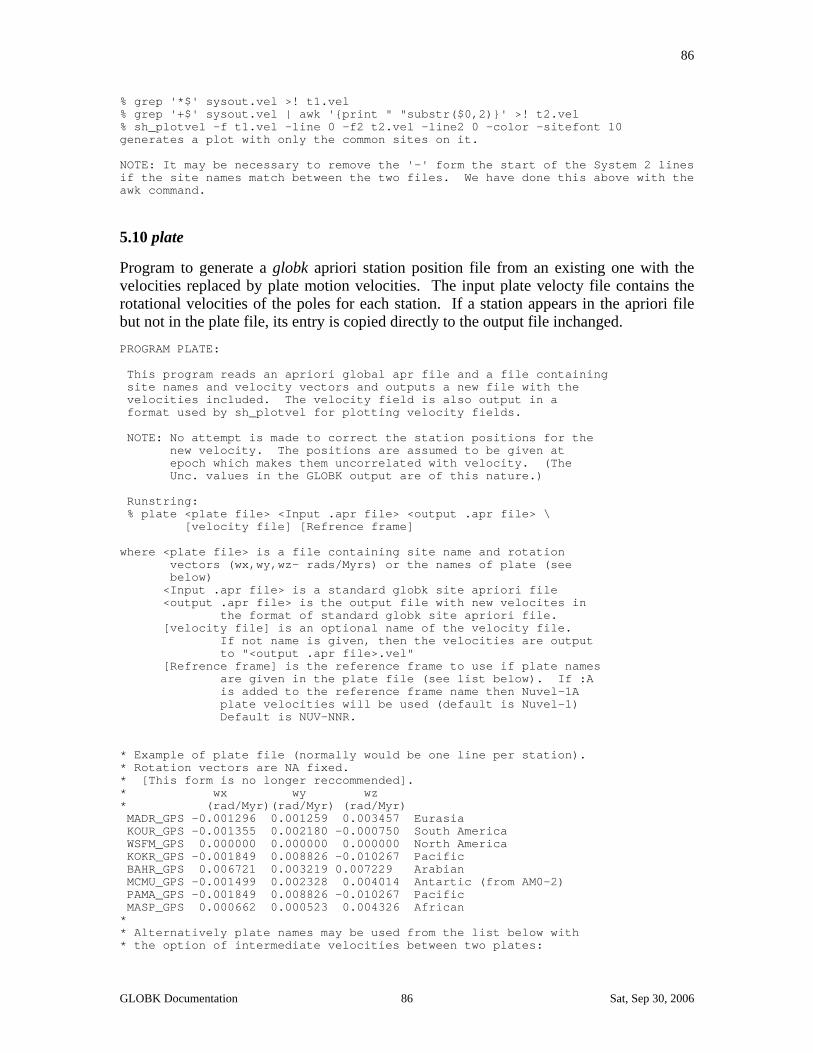
86

% grep '*$' sysout.vel >! t1.vel % grep '+$' sysout.vel | awk '{print " "substr($0,2)}' >! t2.vel % sh_plotvel -f t1.vel -line 0 -f2 t2.vel -line2 0 -color -sitefont 10 generates a plot with only the common sites on it. NOTE: It may be necessary to remove the '-' form the start of the System 2 lines if the site names match between the two files. We have done this above with the awk command.

5.10 plate

Program to generate a globk apriori station position file from an existing one with the velocities replaced by plate motion velocities. The input plate velocty file contains the rotational velocities of the poles for each station. If a station appears in the apriori file but not in the plate file, its entry is copied directly to the output file inchanged. PROGRAM PLATE: This program reads an apriori global apr file and a file containing site names and velocity vectors and outputs a new file with the velocities included. The velocity field is also output in a format used by sh_plotvel for plotting velocity fields. NOTE: No attempt is made to correct the station positions for the new velocity. The positions are assumed to be given at epoch which makes them uncorrelated with velocity. (The Unc. values in the GLOBK output are of this nature.) Runstring: % plate <plate file> <Input .apr file> <output .apr file> \ [velocity file] [Refrence frame] where <plate file> is a file containing site name and rotation vectors (wx,wy,wz- rads/Myrs) or the names of plate (see below) <Input .apr file> is a standard globk site apriori file <output .apr file> is the output file with new velocites in the format of standard globk site apriori file. [velocity file] is an optional name of the velocity file. If not name is given, then the velocities are output to "<output .apr file>.vel" [Refrence frame] is the reference frame to use if plate names are given in the plate file (see list below). If :A is added to the reference frame name then Nuvel-1A plate velocities will be used (default is Nuvel-1) Default is NUV-NNR. * Example of plate file (normally would be one line per station). * Rotation vectors are NA fixed. * [This form is no longer reccommended]. * wx wy wz * (rad/Myr)(rad/Myr) (rad/Myr) MADR_GPS -0.001296 0.001259 0.003457 Eurasia KOUR_GPS -0.001355 0.002180 -0.000750 South America WSFM_GPS 0.000000 0.000000 0.000000 North America KOKR_GPS -0.001849 0.008826 -0.010267 Pacific BAHR_GPS 0.006721 0.003219 0.007229 Arabian MCMU_GPS -0.001499 0.002328 0.004014 Antartic (from AM0-2) PAMA_GPS -0.001849 0.008826 -0.010267 Pacific MASP_GPS 0.000662 0.000523 0.004326 African * * Alternatively plate names may be used from the list below with * the option of intermediate velocities between two plates:


87

pie1_gps nafd mojm_gps nafd 0.25 pcfc * The latter form using NAFD velocity plus 25% of the difference * between PCFC and NAFD. (nafd 1.0 pcfc is the same as pcfc) The following frame names are supported: PCFC, COCO, NAZC, CARB, SAFD, ANTA, INDI, AUST, AFRC, ARAB, EURA, NAFD, JUAN, PHIL, NUV-NNR, AM-02, ITRF93 Adding a :A to the name will scale the rate to the NUVEL_1A model.


Documents

Reference Manual - Geophysics at Georgia Techgeophysics.eas.gatech.edu/.../MGM/GAMIT/GLOBK_Ref_10.3.pdfinterface with GAMIT (for GPS) and CALC/SOLVE (for VLBI), there is little intrinsic