1

RECOUP Working Paper No. 38

Economic Returns to Schooling and Skills – An Analysis of India and Pakistan

Monazza Aslam, Department of Economics, University of Oxford Geeta Kingdon, Institute of Education, University of London Anuradha De and Rajeev Kumar, Collaborative Research and Dissemination (CORD), India

December 2010

2

Economic Returns to Schooling and Skills - An analysis of India and Pakistan

by

Monazza Aslam*, Anuradha De, Geeta Kingdon and Rajeev Kumar

Abstract

This paper investigates the economic (i.e. labour market) outcomes of education for individuals in India and Pakistan. The labour market benefits of education accrue both from education/skills promoting a person’s entry into the more lucrative occupations and by raising earnings within any given occupation. Our research looks at both these channels of effect from education onto economic well-being. This is done using data from two unique purpose-designed comparative surveys of more than 1000 households in India and Pakistan, collected in 2007 and 2008. Multinomial Logit estimates of occupational attainment reveal how years of education and the quality of education determine occupational choice. We estimate the returns to the ‘quantity’ and the ‘quality’ of schooling in different occupations (wage employment, self-employment and agricultural self-employment). The paper also examines the shape of the education-earnings relationship as a way of testing the poverty reducing potential of education. Much of the analysis is done by gender and we ask whether education lowers the gender gap in earnings. Finally, the paper estimates the returns to knowing ‘English’ in the labour markets of the two countries.

Key Words: rates of return, schooling, cognitive skills, English language skills, gender, India, Pakistan

JEL codes: I21, J16, J24.

*Corresponding Author: Department of Economics, University of Oxford, Manor Road, Oxford, OX1 3UQ, United Kingdom, Telephone: +44-1865-271089. monazza.aslam@economics.ox.ac.uk

Geeta Kingdon – Institute of Education, University of London, UK.

Anuradha De – Collaborative Research and Dissemination, India

Rajeev Kumar – Collaborative Research and Dissemination, India

This paper forms part of the Research Consortium on Educational Outcomes and Poverty (RECOUP). Neither DFID nor any of the partner institutions are responsible for any of the views expressed here.For details of the objectives, composition and work of the consortium see: www.educ.cam.ac.uk/RECOUP

3

1. Introduction

This study investigates the economic outcomes of education and skills in India and Pakistan. The

two countries started life as one - the Indian Subcontinent - until Partition in 1947. Since then, the

development trajectories of the two countries have been dramatically different. Some basic statistics from

the World Bank1 for the period around 2002 to 2008 highlight the different paths the two countries have

taken in recent years. India's average annual growth rate of GDP in 2007 was an impressive 9.1 per cent

compared to a more modest 5.7 per cent for Pakistan in the same year. The proportion of the adult

population (aged 15 and above) deemed literate was 66 per cent in India compared to 54 per cent in

Pakistan and compared to a South Asian average of 63 per cent. In many respects, India appears to be

performing well above the regional average while Pakistan's performance has been consistently poorer.

This is most apparent in schooling – the gross primary enrolment rate in India was 113 percent compared

to only 85 per cent in Pakistan and compared to a South Asian average of 108 per cent. However, the

similarities between the two countries are far greater than the differences. For one, the countries share a

common culture. Both India and Pakistan are highly polarized along economic, gender, geographic,

religious, and ethnic lines. These fragmentations are more apparent in the labour market than elsewhere.

For instance, women's access to the labour market is consistently limited in both countries. When in the

labour market, their choices are limited to certain occupations. It is therefore not surprising that women's

earnings are substantially less than men's in both countries. In spite of an overall Indian advantage, several

Indian states are very similar to those in Pakistan in terms of development indicators.

As mentioned before, the key objective of this study is to investigate economic outcomes of

education and skills in India and Pakistan. The labour market benefits of education and skills may accrue

both via promoting a person’s entry into lucrative occupations and, conditional on occupation, via raising

earnings. This association is investigated by analyzing the relationship between schooling and cognitive

skills on the one hand, and occupational choice and earnings on the other. We also go one step further and

analyze the role of English knowledge on occupational attainment and economic return in the case of male

and female wage workers in the two countries.

The study is motivated by three major questions that have not been answered satisfactorily so far

about the effects of education on people’s economic outcomes in developing countries. Firstly, while

many studies estimate economic rates of return to education in order to examine how much education is

rewarded in the labour market, almost all these studies have been on the profitability of education among

wage workers (see for instance Aslam, 2009b; or Aslam, Bari and Kingdon, 2008). Earnings regressions

have not been attempted for self employment mainly because large scale data sources usually do not

collect information on earnings of the self employed. And even when earnings are available it is “difficult

1 Available from www.worldbank.org

4

to separate the contribution due to physical capital, human capital and the reward for risk and uncertainty

bearing” (Duraisamy, 2002, p 610). In Pakistan, Kingdon and Soderbom’s (2007) work is one of the first

attempts to estimate earnings functions for the self employed and agricultural workers; they used the

Pakistan Integrated Household Survey (PIHS) data, though data on all key variables (such as capital stock)

were not available. One recent study by Bhandari and Bordoloi (2006) in India looked at waged and self-

employed workers but the analysis was done for all workers together and not separately for these

categories. This is important because wage work is a small and often shrinking part of the labour market in

developing countries. As a result, the question: 'does education play a productivity-enhancing and

poverty-reducing role in the expanding sectors of the labour market?' often remains unaddressed. In this

survey we have collected data on earnings of individuals in all occupations. So we are able to estimate

how rewarding education is not only in wage employment but also in self-employment and in agriculture.

Secondly, it is increasingly thought that it is not mere completion of years of schooling but what is

learnt at school that matters to productivity and earnings. There is considerable evidence in developed

countries, and to some extent in developing countries, to substantiate the claim that cognitive skills are

important determinants of increased earnings (this literature is summarized in Hanushek, 20052 and more

recently in Hanushek and Woessmann, 2007). In this paper we have added to this body of evidence

through a similar exercise, where we have estimated the economic returns to cognitive skills and

compared these with the economic returns to years of schooling.

Thirdly, while there is anecdotal evidence in both India and Pakistan that there are sizeable

economic returns to English Language3, lack of data has meant that this has not been empirically tested,

particularly in Pakistan. Our rich data allow us to look at the impact of English Language on earnings in

wage work for both males and females. Both India and Pakistan have a rich Colonial heritage. The British

rule between 1757-1947 left a strong legacy. While Hindi and Urdu are the national languages of India

and Pakistan respectively, English remains the 'official' language in Pakistan and India (for

communication between the states/provinces and the federal government), and is used much in the skilled

part of business and industry. From an individual's perspective English language knowledge remains

advantageous as it is considered a necessary tool for improved economic prospects. There are two studies

by Bhandari and Bordoloi (2006, p 3899) and Azam, Chin and Prakash (2010) on India, both of which

find that knowledge of the English language has a significant association with earnings. Incomes are 2 Hanushek (2005) cites 3 US studies showing quite consistently that a one standard deviation increase in mathematics test performance at the end of high school translates into 12 per cent higher annual earnings. Hanushek also cites three studies from the UK and Canada showing strong productivity returns to both numeracy and literacy skills. Other studies cited indicate substantial returns to cognitive skills in developing countries such as Ghana, Kenya, Tanzania, Morocco, Pakistan and South Africa. 3 Aslam (2006) in her study of schools in (Lahore) Pakistan found numerous parents suggesting that they were opting for the pricier private schools as they are 'English Medium' and would give their children the opportunity to learn English and get ahead in life.

5

between 13 and 34% higher among workers that speak English, depending on the level of fluency. To our

knowledge, there has not been a basic descriptive analysis of knowledge of English skills in Pakistan let

alone any estimates of economic returns4. The RECOUP data allows us to estimate for the first time the

association of English Language skills with occupational attainment and economic returns for wage

workers in Pakistan.

In addition to the aforementioned, we also (a) consider the pattern of returns to different levels of

education – is the pattern concave as is conventionally believed? (b) compare the labour market rewards

of education for men and women in wage work; in particular, whether education lowers the gender gap in

earnings, and how (via increasing women’s chances of participation in more lucrative work or via higher

returns to education for women).

The paper is structured as follows: section 2 discusses the empirical methodology used and

section 3 describes the data and its key features. Section 4 discusses results and is divided into three

subsections: the first part focuses on a graphical analysis of how education and cognitive skills determine

occupational outcomes; the second examines the relationship between earnings and education; and the

third section discusses the relationship between earnings and cognitive skills. Section 5 concludes.

2. Empirical Methodology

The effect of education on earnings may operate through several channels such as through improving

access to lucrative occupations or, conditional on occupational attainment, by raising earnings within any

given occupation (Kingdon and Söderbom 2007, Aslam, Kingdon and Söderbom 2008, Aslam, Bari and

Kingdon 2008). In this study, we explore the relationship between education and occupational attainment

as well as the total effect of education on earnings. This is done by estimating Multinomial Logit (MNL)

models of occupational attainment and Mincerian earnings functions.

The analysis begins by estimating MNL models. All individuals in the labour market in both countries

are classified into one of seven occupational categories: out of the labour force (OLF), unemployed,

unpaid family workers, agricultural self-employed, non-farm self-employed, casual wage employees and

regular wage employees. Unemployed individuals are those who seek employment and are available for it,

while OLF individuals are those who do not seek employment, such as housewives, full-time students and

the retired. In South Asia, often more than one family member of a household may work in their family

farm or non-farm household enterprise. In this case, we define the person reported to be the primary

worker/decision maker to be self-employed. If any other family member reports getting separate earnings

from the work, they are considered wage workers and the rest are considered unpaid family labour. The

5 Annual ASER Reports (2007 onwards) report English skills of school going children in India

6

questionnaire used in both countries allows us to distinguish between the two types of wage work on the

basis of how wages are received: regular wage workers are defined as those who report receiving monthly

earnings while casual workers report a daily or weekly wage.

The second part of the study estimates standard Mincerian earnings functions:

LnYi = β0 + β1Si + β2Xi + εi (1)

In the empirical analysis, earnings regressions are based on data from three labour market sub-

sectors, namely wage employment, self employment, and agriculture. Amongst the wage employed, we

have individual data on earnings as well as on the explanatory variables. So in (1), LnYi is the natural log

of annual earnings of individual i, Si measures years of completed schooling (or literacy, numeracy or

English language test scores), Xi is a vector of observed characteristics of individual i (such as age and its

square) and εi is an individual-specific error term. In this specification, β1 reflects a return to schooling,

skills or English Language depending on whether Si measures years of completed schooling or test scores.

However self employment and agriculture are often 'household enterprises' in South Asia and

several individuals in a family may contribute their time and effort and the earnings from these enterprises

may be shared. Because the social norm in South Asia is to report the oldest male family member as the

‘primary’ worker, it was difficult to identify the main worker/decision-maker in our data. Therefore,

earnings functions have been estimated at the household level, and household-level characteristics are

averaged for estimating Mincerian earnings for these activities. As a household may engage in more than

one self employment activity, each self employment activity in the sample households is considered a

single observation5. In order to identify the parameters in (1) the explanatory variables were aggregated so

that they were defined at the same level of aggregation as the dependent variable. For the dependent

variable, earnings were averaged over the number of family workers. Similarly, mean values were

calculated for the other explanatory variables (age and education of members employed in that enterprise)

within the household. Thus, variables of equation (1) are reinterpreted in the case of self-employment –

LnYi is the natural log of average annual earnings per person of the unpaid family labour and main self

employed in observation i, Si measures their average years of completed schooling, Xi is a vector of

observed characteristics in observation i and εi is an observation-specific error term. In this specification,

β1 reflects marginal return to schooling among self-employed persons.

As the primary objective of the paper is to estimate the total returns to education, the variables

included as regressors in MNL and earnings function models are selected accordingly. The basic 5 It is important to note that about 6 (8) percent of households report more than one self employment activity in India (Pakistan). In some of these households, unpaid labour may be working in more than one of these. So a small amount of incorrect assignment of self employment to unpaid family workers couldn’t be avoided.

7

regressions contain a very small set of control variables. In MNL models the vector of regressors is similar

for India and Pakistan. It contains age (and the quadratic of age), years of completed schooling, dummies

for state, and location, number of individuals in the household aged less than 15, number of adults in the

household aged more than 60 and a dummy variable measuring whether the individual is married or not.

Religion and caste are additional controls used in the India regressions. As we intend to determine the

effects of both years of schooling and that of cognitive skills on occupational attainment we also include

cognitive test scores in some MNL models.

The regressors of baseline earnings functions differ slightly depending on the country of

estimation: in both countries we include age, age squared, gender, and regional and provincial fixed

effects. In India, we also control for religion and caste as they are particularly important fault-lines in the

labour market. With respect to the effect of these variables on earnings we allow for a degree of flexibility

by estimating the earnings regressions for waged employees separately for men and women and pooled

estimates for all persons. Education is measured by years of completed education or alternatively by the

cognitive test scores.

We start by estimating Ordinary Least Squares (OLS) models of earnings functions to provide

some baseline results. OLS estimates potentially suffer from two major biases - sample selectivity and

endogeneity (omitted variable) bias. Sample selectivity bias arises due to estimating the earnings function

on separate sub-samples of workers, each of whom may not be a random draw from the population. This

violates a fundamental assumption of the least squares regression model. While modelling occupational

outcomes can be a useful exercise in its own right – suggesting the way in which education, skills and

household demographics influence people’s decisions to participate in different types of employment – it

is also needed for the consistent estimation of earnings functions. Modelling participation in different

occupations is the first step of the Heckman procedure to correct for sample selectivity: probabilities

predicted by the occupational choice model are used to derive the selectivity term that is used in the

earnings function. Following Heckman (1979), the earnings equations can be corrected for selectivity by

including the inverse of Mills ratio λi as an additional explanatory variable in the earnings function.

The problem of endogenous sample selection is akin to the problem of endogeneity bias. Endogeneity

bias arises if workers’ unobserved traits, which are in the error term, are systematically correlated both

with included independent variables and with the dependent variable (earnings). For instance, if worker

ability is positively correlated with both education/cognitive skills and with earnings then any positive

coefficient on education (or cognitive skills) in the earnings function may simply reflect the cross-

sectional correlation between ability on the one hand and both education/skills and earnings on the other,

rather than representing a causal effect from education/skills onto earnings. There are several approaches

to addressing endogeneity bias such as including 'ability' measures in earnings functions, instrumental

8

variable approaches and household fixed effect methods (see Aslam, Bari and Kingdon 2008 for this

analysis on Pakistan).

In this study, we use household fixed-effects in a bid to address potential endogeneity of schooling.

The idea is to use observations from different individuals within the same family to estimate a ‘household

fixed effects’ earnings equation. To the extent that unobserved traits are shared within the family, their

effect will be netted out in a family differenced model. For instance, the error term ‘difference in ability

between members’ will be zero if it is the case that ability is equal among members. While it is unlikely to

be the case that unobserved traits are identical across family members, it is likely that they are much more

similar within a family than across families and, as such, family fixed-effects estimation reduces

endogeneity bias without necessarily eliminating it entirely. The key problem in using this approach is that

it imposes quite stringent requirements on the data. In our case, this estimation of earnings functions is

also possible only for waged workers as agriculture and non-farm self employment are considered as

household enterprises. Hence, while we report and discuss endogeneity-corrected results, our main

findings in this paper are based on OLS estimates and we recognize while these estimates may not be

error-free, they do present a lower bound on returns estimates.

3. Data and Descriptive Statistics

This study primarily uses data from two comparative household surveys conducted in Pakistan

(November 2006 to March 2007) and in India (October 2007 to January 2008). The surveys were part of a

larger five-year DFID-funded project - the Research Consortium on Educational Outcomes and Poverty

(RECOUP). As part of a multi-country study, the survey instruments used in the household surveys were

almost identical with very minor differences to allow for cultural and institutional variations across the

two countries.

In Pakistan, the purpose-designed household survey was administered to 1194 urban and rural

households. Households were selected randomly through stratified sampling from 9 districts in two

provinces – Punjab and the-then North West Frontier Province (NWFP)6. In India, information was

collected from more than 1000 households in 18 villages and 6 towns, selected through stratified sampling

from 6 districts in two states - Madhya Pradesh (MP) and Rajasthan.

The RECOUP survey collected rich information on previously unavailable variables. While the roster

captured basic demographic, anthropometric, education and labour market status information on all

6 This province is now called Khyber-Pakhtunkhwah (KP). The districts sampled in Punjab included: Rahimyar Khan, Khanewal, Sargodha, Kasur, Attock and Chakwal and Swat, Charsadda and Haripur were sampled from KP. The surveyed districts in India were Alwar, Pali and Dhaulpur in Rajasthan, and Dewas, Ratlam and Shajapur in M.P.

9

resident household members in the sampled households (more than 8000 individuals in Pakistan and more

than 6000 in India), detailed individual-level questionnaires were administered only to those aged between

15 and 60 years. Some 4907 individual-level questionnaires were filled in Pakistan and 3588 in India.

These individuals were also administered tests of literacy, numeracy, health knowledge and English

language. For literacy and numeracy two types of instruments were used to capture ‘basic order’ skills and

‘higher order’ skills. In our analysis we have used scores of ‘short literacy test’ and ‘short numeracy test’,

each consisting of 5 questions. The English Language skills test consisted of 19 questions.

Table 1 shows summary statistics for labour market status by gender. Workers may have multiple

occupations and are classified by their self- reported principal work status7. The extent of gender

asymmetry in the distribution of the labour force is striking in both countries but more so in Pakistan than

in India. A significant majority of women are not economically active. In Pakistan, about 70 per cent

women are out of the labour force compared to 18 per cent men. This asymmetry is considerably smaller

in India – about 40 per cent women are out of the labour force compared to about 12 per cent men. Even

among women who are in the labour force in India, very few are in remunerative occupations. Nearly two

thirds of the economically active women in India work as unpaid family labour in family based agriculture

or enterprise and about a fifth are casual workers. In Pakistan, a large proportion of women report being

unemployed. However, interestingly, when women are in the labour market in Pakistan, they are more

likely to be engaged in self-employment activities and regular work compared to women in India. This

difference cannot be generalized across the two countries because while in Pakistan the sample chose a

highly progressive province (Punjab), in India two of the poorest and relatively more backward states

were selected. Finally, among men who are economically active, wage employment absorbs the largest

share in both countries, though a larger share of men report doing regular (as opposed to casual) waged

work in Pakistan than in India.

Table 2 summarizes some key statistics for different occupational groups in the two countries. The

table has two alternative sets of statistics – the upper part gives the average education levels for all

occupational groups where the reported principal worker in the household is considered to be the non-farm

self employed or in agriculture. An alternate calculation is attempted in the lower part of the table where

unpaid family workers are included in the occupation they work in (agriculture or non-farm self

employment). Education levels and cognitive skills scores are averaged over them. Average earnings are

also calculated similarly – the unpaid family workers are assigned an earnings value of zero instead of

missing earnings and the total earnings of everyone in this new category are averaged over the total

number of workers. Both for India and Pakistan we find high education levels (and test scores) in both 7 Those who are self employed or report agricultural work with low earnings or are unpaid family workers in household farm or enterprise, and who also have to do wage work in lean or off season, may be categorized as wage workers in this analysis.

10

regular work and non-farm self employment. It is much lower in agriculture and casual work, in both

countries. Education levels are low for unpaid family workers as well. The high level of education of

individuals reportedly out of the labour force in India is also remarkable, suggesting ‘queuing up’ in the

absence of good work opportunities. Males are seen to dominate in all paid work. Another notable feature

in both countries is urban dominance in lucrative types of work namely, regular work and non-farm self-

employment.

In the lower portion of the table the calculations are differently done and education levels are now

much lower for those in non-farm self employment and agriculture. The earnings in all occupations are

mirrored by completed years of schooling and by literacy and numeracy skills, and the only exception are

casual workers in Pakistan whose earnings are relatively quite high given their education levels. The mean

earnings in agriculture are low, even lower than that of casual wage workers in both India and Pakistan.

This hierarchy in earnings across occupation-types shows a close correspondence with years of education.

However, given the very low level of education among casual workers, their earnings seem to be

unusually high in Pakistan. Regular work and non-farm self employment, two of the more remunerative

occupations, also notably have the highest proportion of male workers in India.

Table 3 summarises key statistics by gender. As noted before, women's participation in the labour

force is generally low in both countries, but the gender difference is particularly stark in agriculture and in

non-farm self employment. In Pakistan, women simply do not report agricultural work and in India they

primarily work in agriculture as unpaid family labour. The gender gap in education and in literacy and

numeracy skills remains very sharp in all occupation groups in both India and Pakistan – the only

exception is in regular wage work. Similarly when we look at differences in earnings of wage workers we

note that women's wages in casual work in India are abysmally low – a matter of grave concern as casual

work is the main income earning occupation for women in the sampled regions. In contrast, regular waged

work is one occupation where women are fairly equal to males in terms of education, skills and earnings

in both India and in Pakistan. But very few women are in this sector. Clearly education and skills have

some association with occupational choice and earnings. However, this is an empirical question and we

turn to this in the next section.

4. Empirical Findings

4.1 Years of Schooling and Skills and Occupational Attainment

This sub-section investigates whether one of the ways in which the labour market benefits of

human capital accrue is via promoting entry into more lucrative occupations. This is done by looking at

11

the effect of education and of literacy, numeracy and English language skills on occupational outcomes8.

As discussed before, we define seven 'occupations' using the data. Because social norms and work

opportunities are likely to be very different in rural and urban areas, the analysis is done separately by

gender in both locations.

The analysis in this subsection is undertaken by means of simple, parsimoniously specified

Multinomial Logit (MNL) models (see section 3). While MNL models are clearly appropriate tools for

modeling multiple occupational choices, the coefficients are hard to interpret. Hence, while we report

some key marginal effects from MNL regressions in the Appendix, we largely discuss results from the

graphical analysis that is based on underlying MNL regressions. The regression results are suppressed due

to space constraints (see Appendix P4 for example).

We begin by modeling occupational outcomes by gender and by region on years of education. The

partial effects presented in Table I1 and P1 indicate the strong impact of education on probabilities of

being in particular occupations, more so in India than in Pakistan.9

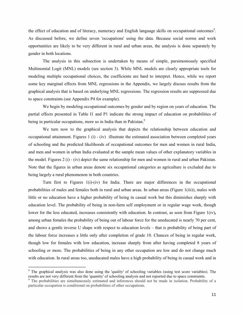
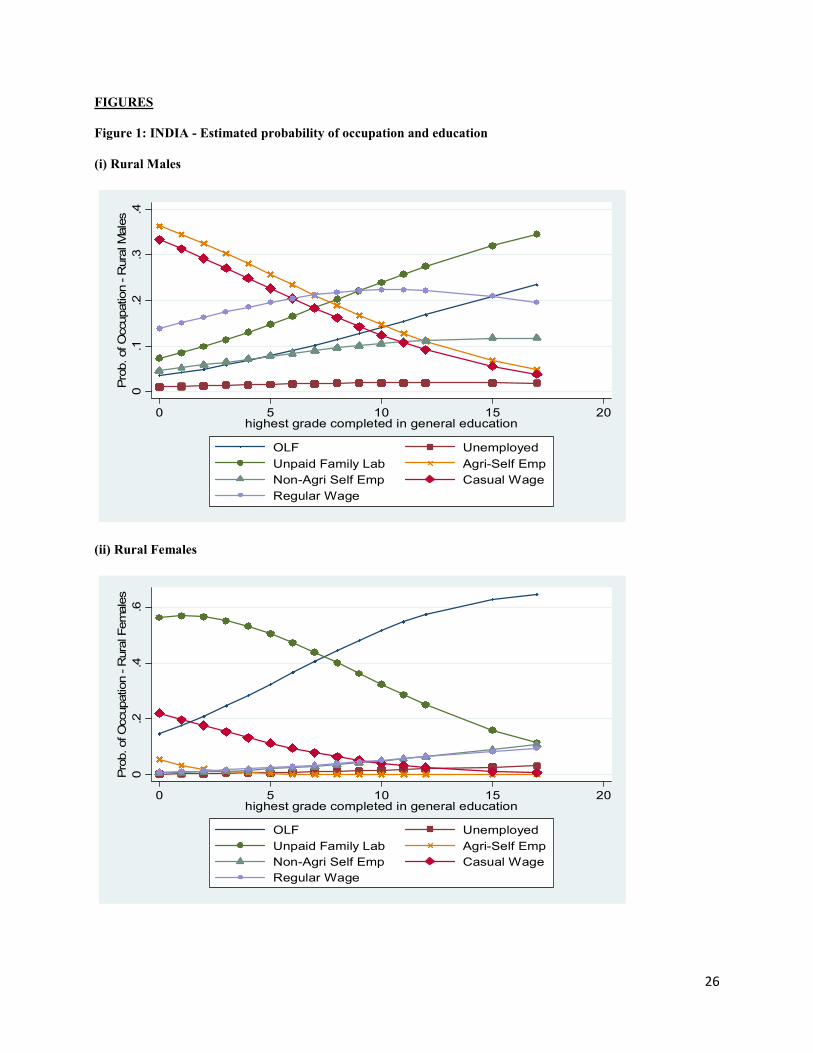
We turn now to the graphical analysis that depicts the relationship between education and

occupational attainment. Figures 1 (i) - (iv) illustrate the estimated association between completed years

of schooling and the predicted likelihoods of occupational outcomes for men and women in rural India,

and men and women in urban India evaluated at the sample mean values of other explanatory variables in

the model. Figures 2 (i) - (iv) depict the same relationship for men and women in rural and urban Pakistan.

Note that the figures in urban areas denote six occupational categories as agriculture is excluded due to

being largely a rural phenomenon in both countries.

Turn first to Figures 1(i)-(iv) for India. There are major differences in the occupational

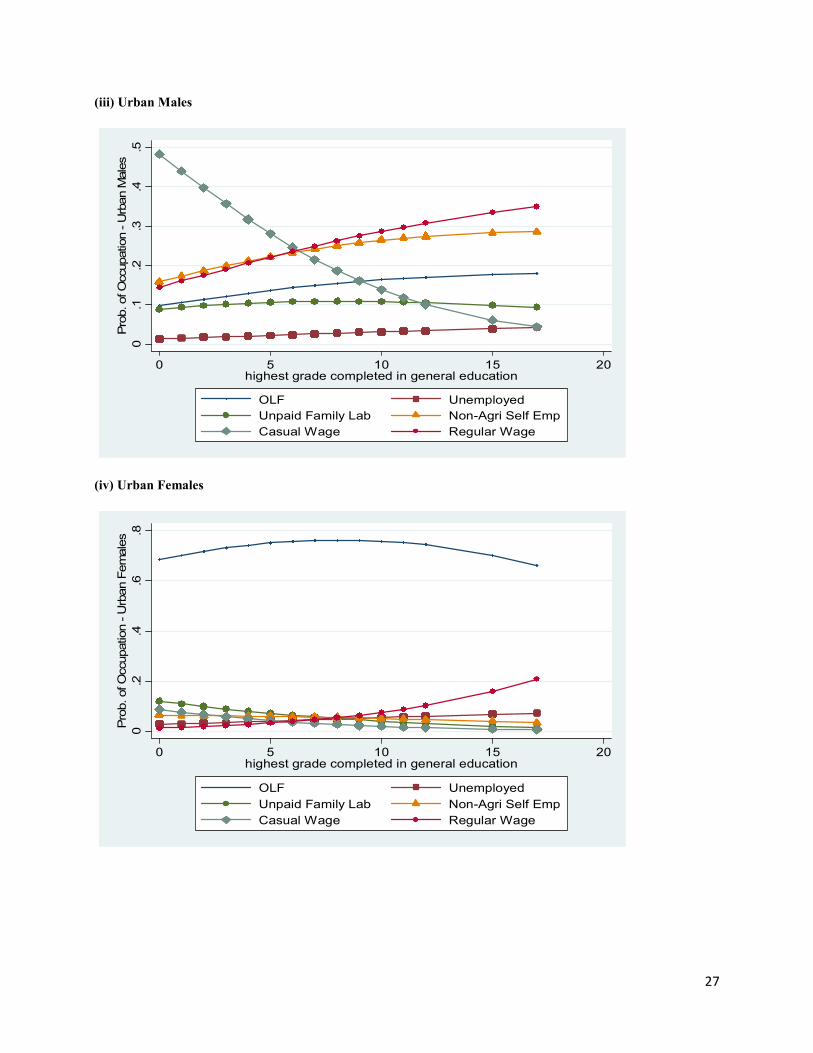
probabilities of males and females both in rural and urban areas. In urban areas (Figure 1(iii)), males with

little or no education have a higher probability of being in casual work but this diminishes sharply with

education level. The probability of being in non-farm self employment or in regular wage work, though

lower for the less educated, increases consistently with education. In contrast, as seen from Figure 1(iv),

among urban females the probability of being out of labour force for the uneducated is nearly 70 per cent,

and shows a gentle inverse U shape with respect to education levels – that is probability of being part of

the labour force increases a little only after completion of grade 10. Chances of being in regular work,

though low for females with low education, increase sharply from after having completed 8 years of

schooling or more. The probabilities of being in any other occupation are low and do not change much

with education. In rural areas too, uneducated males have a high probability of being in casual work and in

8 The graphical analysis was also done using the 'quality' of schooling variables (using test score variables). The results are not very different from the 'quantity' of schooling analysis and not reported due to space constraints. 9 The probabilities are simultaneously estimated and inferences should not be made in isolation. Probability of a particular occupation is conditional on probabilities of other occupations.

12

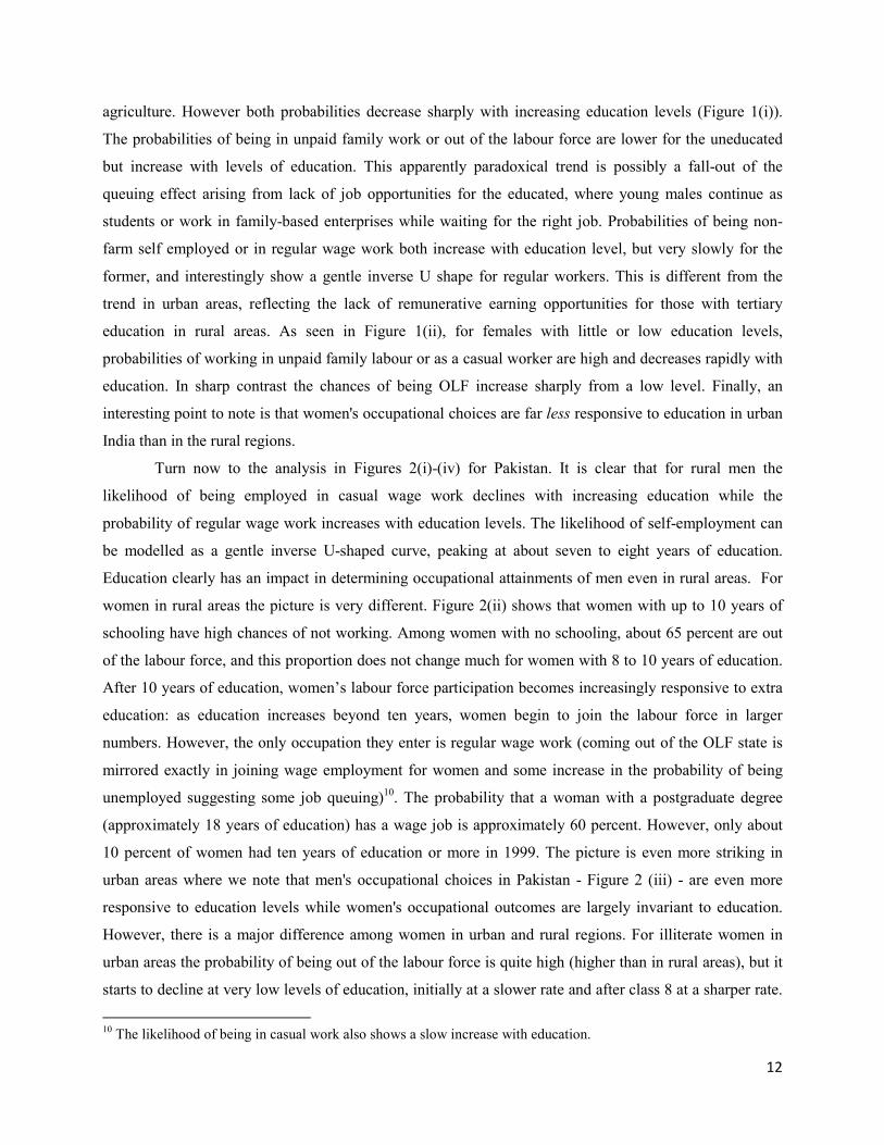
agriculture. However both probabilities decrease sharply with increasing education levels (Figure 1(i)).

The probabilities of being in unpaid family work or out of the labour force are lower for the uneducated

but increase with levels of education. This apparently paradoxical trend is possibly a fall-out of the

queuing effect arising from lack of job opportunities for the educated, where young males continue as

students or work in family-based enterprises while waiting for the right job. Probabilities of being non-

farm self employed or in regular wage work both increase with education level, but very slowly for the

former, and interestingly show a gentle inverse U shape for regular workers. This is different from the

trend in urban areas, reflecting the lack of remunerative earning opportunities for those with tertiary

education in rural areas. As seen in Figure 1(ii), for females with little or low education levels,

probabilities of working in unpaid family labour or as a casual worker are high and decreases rapidly with

education. In sharp contrast the chances of being OLF increase sharply from a low level. Finally, an

interesting point to note is that women's occupational choices are far less responsive to education in urban

India than in the rural regions.

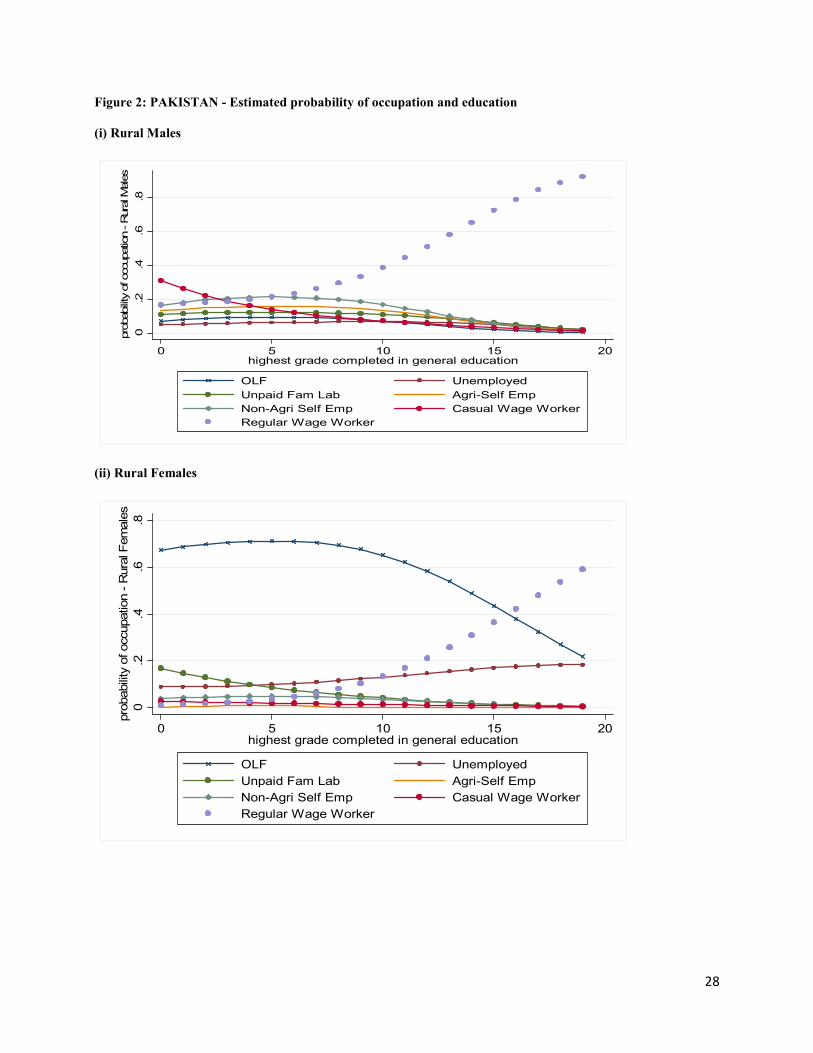
Turn now to the analysis in Figures 2(i)-(iv) for Pakistan. It is clear that for rural men the

likelihood of being employed in casual wage work declines with increasing education while the

probability of regular wage work increases with education levels. The likelihood of self-employment can

be modelled as a gentle inverse U-shaped curve, peaking at about seven to eight years of education.

Education clearly has an impact in determining occupational attainments of men even in rural areas. For

women in rural areas the picture is very different. Figure 2(ii) shows that women with up to 10 years of

schooling have high chances of not working. Among women with no schooling, about 65 percent are out

of the labour force, and this proportion does not change much for women with 8 to 10 years of education.

After 10 years of education, women’s labour force participation becomes increasingly responsive to extra

education: as education increases beyond ten years, women begin to join the labour force in larger

numbers. However, the only occupation they enter is regular wage work (coming out of the OLF state is

mirrored exactly in joining wage employment for women and some increase in the probability of being

unemployed suggesting some job queuing)10. The probability that a woman with a postgraduate degree

(approximately 18 years of education) has a wage job is approximately 60 percent. However, only about

10 percent of women had ten years of education or more in 1999. The picture is even more striking in

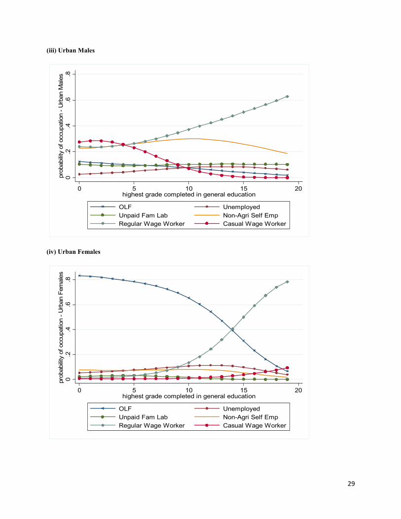
urban areas where we note that men's occupational choices in Pakistan - Figure 2 (iii) - are even more

responsive to education levels while women's occupational outcomes are largely invariant to education.

However, there is a major difference among women in urban and rural regions. For illiterate women in

urban areas the probability of being out of the labour force is quite high (higher than in rural areas), but it

starts to decline at very low levels of education, initially at a slower rate and after class 8 at a sharper rate.

10 The likelihood of being in casual work also shows a slow increase with education.

13

But for women in rural areas the probability of being out of labour force is noticeable only after 10 years

of education.

That occupational outcomes of education are so different for men and women suggests the strong

influence of culture, conservative attitudes, and gender division-of-labour norms in Pakistan. Only

education beyond ten years in rural areas (and about 6-8 years in urban areas) begins to counter the effects

of culture, but barely 18 percent of women in 2007 are fortunate enough to have at least ten years of

education. This provides one element of the answer to one of the key questions in this study: education has

only limited potential to effect gender equality in the labour market because, as a result of cultural norms,

occupational choices are invariant with respect to education up to the end of lower secondary education,

and only a small minority of Pakistani women have greater than ten years of education.

Summarizing, the graphical analysis in India and in Pakistan reveals that the quantity of education

is a critical determinant of occupational choice – higher education usually increases the probability of

being in more remunerative occupation. But the influence of education is modified by labour market

constraints – as seen in a weaker relationship in rural areas, and by social norms as seen from the changes

in the probability of females being out of labour force in both areas. The constraints to women's

participation are particularly pronounced in Pakistan where we observe women's occupational choices

being highly limited and largely invariant to education levels. These differences by gender across the two

countries and by region within them are perhaps most striking from a policy perspective.

Appendix Tables I3 and P3 present the marginal effects of literacy, numeracy and English

language skills by gender on the likelihood of being in different labour market states in a bid to understand

how they impact occupational choice. The results are not discussed here due to space constraints. The key

finding in both countries is that skills appear to be important determinants of occupational choice. A better

understanding of what is happening in the labour market is possible only by looking at how the rewards to

schooling and skills differ in India and in Pakistan and we turn to this in the next sub-section.

4.2 Years of Schooling and Earnings

In this sub-section we start by investigating how the wage increment from each extra year of

schooling compares across the different occupations - agriculture, self employment and wage work and,

when possible, by gender. This is done by estimating and comparing the marginal rate of return using the

familiar Mincerian earnings function approach where the coefficient on ‘years of schooling’ measures the

rate of return to each additional year of schooling acquired. Unless otherwise stated, we always control for

age, age squared and region (urban dummy, except for agricultural workers) and province fixed effects.

The regressions in India always control for religion and caste. The dummy variable for religion is defined

as Hindu having a value 1 and 0 otherwise. For general caste and other backward caste persons, the caste

14

dummy takes the value of 1 and for scheduled caste and scheduled tribe individuals it takes the value of 0.

In the next sub-section, measures of skills – literacy and numeracy – as well as English Language test

scores are included rather than years of schooling in a bid to estimate any potential returns to skills.

As explained earlier, the Mincerian function is estimated at the individual level for wage

workers11. Regressions for male-female pooled models for wage workers always include the gender

dummy (MALE, equals 1 if male, 0 otherwise). Separate regressions for males and females are also

estimated for wage workers to allow for the vector of coefficients to differ by gender. For persons reported

to be working as farmers and as self employed, the earnings functions are modified and estimated at the

household level. Thus, average monthly earnings, average years of education and average age of all

household members working in the enterprise (unpaid family labour and main self employed) are used for

the Mincerian estimations. This does not allow for analysis by gender. Importantly, our data allows us to

control for log of value of fixed capital stock used in both types of self employment, as well as work

intensity measured as average of hours worked per day. In the case of agriculture, we also control for size

of cultivated land. The inclusion of these variables enriches our study as lack of data in the past has meant

these crucial variables have not been controlled for in extant analyses.

Table 4 presents base-line OLS estimates of the Mincerian returns to education for the different

occupations (without and with capital stock and landsize for agriculture and without and with capital stock

for the self employed) in India and Pakistan. Focus first on the India estimates. In all earning regressions

the coefficients of most of the dummy variables are significant (’Hindu’ is the only exception). Average

earnings of SCs and STs are lower in all types of employment. Earnings are also lower for rural workers

as compared to urban workers. The coefficient of state dummy indicates that average earnings in

agriculture are much lower (around 30 percent) in Rajasthan as compared to MP. Controlling for capital

and land size brings this difference down to 14 percent (and makes it insignificant), implying that much of

the earlier difference was due to larger land size and capital investment in MP. In this model the state

dummy also becomes insignificant. Higher returns to agriculture in Madhya Pradesh are not surprising in

this data as the sample areas in the state have more profitable agriculture; average quality of land is better

and cropping pattern is more commercial. In Rajasthan in the absence of profitable farming options and

successive years of drought, people appear to have opted for non-farm sector employment. Average

earnings are higher in Rajasthan for the non-farm self employed and for those in wage work. Among the

casual workers too a larger proportion in MP work in the agricultural sector. As wages in agriculture are

lower than non-farm wages, the average wage earnings in MP is lower than in Rajasthan.

11 Because the number of observations is limited when we disaggregate by gender and by regular/casual wage work, wage earnings functions are estimated only by gender but a wage-work dummy variable is included in Table 4a to determine the impact of casual/regular work.

15

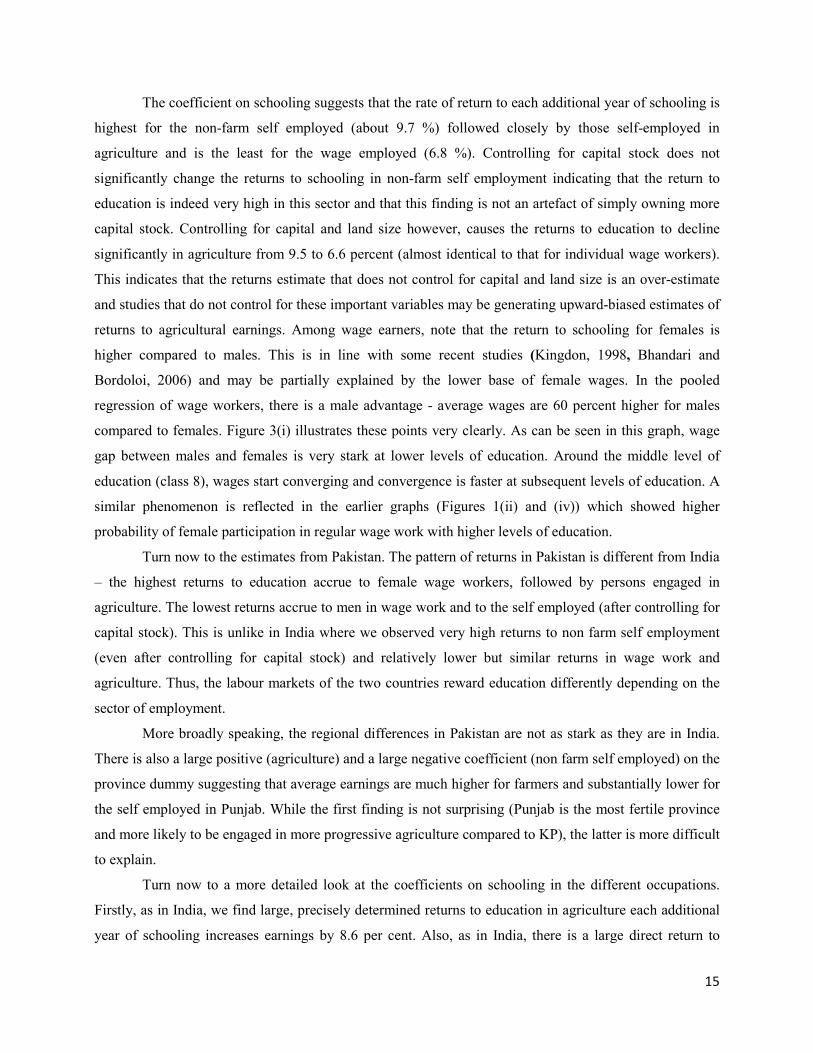
The coefficient on schooling suggests that the rate of return to each additional year of schooling is

highest for the non-farm self employed (about 9.7 %) followed closely by those self-employed in

agriculture and is the least for the wage employed (6.8 %). Controlling for capital stock does not

significantly change the returns to schooling in non-farm self employment indicating that the return to

education is indeed very high in this sector and that this finding is not an artefact of simply owning more

capital stock. Controlling for capital and land size however, causes the returns to education to decline

significantly in agriculture from 9.5 to 6.6 percent (almost identical to that for individual wage workers).

This indicates that the returns estimate that does not control for capital and land size is an over-estimate

and studies that do not control for these important variables may be generating upward-biased estimates of

returns to agricultural earnings. Among wage earners, note that the return to schooling for females is

higher compared to males. This is in line with some recent studies (Kingdon, 1998, Bhandari and

Bordoloi, 2006) and may be partially explained by the lower base of female wages. In the pooled

regression of wage workers, there is a male advantage - average wages are 60 percent higher for males

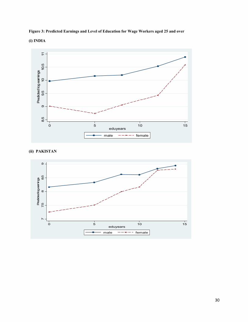
compared to females. Figure 3(i) illustrates these points very clearly. As can be seen in this graph, wage

gap between males and females is very stark at lower levels of education. Around the middle level of

education (class 8), wages start converging and convergence is faster at subsequent levels of education. A

similar phenomenon is reflected in the earlier graphs (Figures 1(ii) and (iv)) which showed higher

probability of female participation in regular wage work with higher levels of education.

Turn now to the estimates from Pakistan. The pattern of returns in Pakistan is different from India

– the highest returns to education accrue to female wage workers, followed by persons engaged in

agriculture. The lowest returns accrue to men in wage work and to the self employed (after controlling for

capital stock). This is unlike in India where we observed very high returns to non farm self employment

(even after controlling for capital stock) and relatively lower but similar returns in wage work and

agriculture. Thus, the labour markets of the two countries reward education differently depending on the

sector of employment.

More broadly speaking, the regional differences in Pakistan are not as stark as they are in India.

There is also a large positive (agriculture) and a large negative coefficient (non farm self employed) on the

province dummy suggesting that average earnings are much higher for farmers and substantially lower for

the self employed in Punjab. While the first finding is not surprising (Punjab is the most fertile province

and more likely to be engaged in more progressive agriculture compared to KP), the latter is more difficult

to explain.

Turn now to a more detailed look at the coefficients on schooling in the different occupations.

Firstly, as in India, we find large, precisely determined returns to education in agriculture each additional

year of schooling increases earnings by 8.6 per cent. Also, as in India, there is a large direct return to

16

capital stock and cultivated land for in agriculture Moreover, as in India, the return to education declines

through inclusion of capital and land size variables for agriculture. The return to agriculture is almost

identical in magnitude to that in India. This finding of a large positive return to agricultural work is

contrary to the notion (hitherto untested in India and Pakistan) that the rewards of education must be lower

in agriculture than in wage employment. These notions are shaped by the small amount of research done

in the early 1980s e.g. by Jamison and Lau in Nepal and by some researchers in the late 1990s in Africa

(Weir and Knight 2006) which suggests very low returns to education agriculture. But the pattern of

agriculture may have changed in recent years in the two countries to more skill-rewarding agriculture as

indeed our findings suggest. Agriculture in the two countries appears to be of a modernising variety12.

The evidence also suggests large positive returns to education among the non-farm self employed

in Pakistan though the returns are not as high as in India. Controlling for capital stock causes the returns to

decline from about 6 per cent to about 4 per cent. As before, this finding clearly highlights the need to

control for capital and suggests that past estimates may have been biased by their failure to control for this

key variable. Moreover, the existence of substantial returns to education in self employment in both India

and Pakistan is welcome news because it suggests that education plays a productivity-enhancing and

poverty reducing role not just in wage employment.

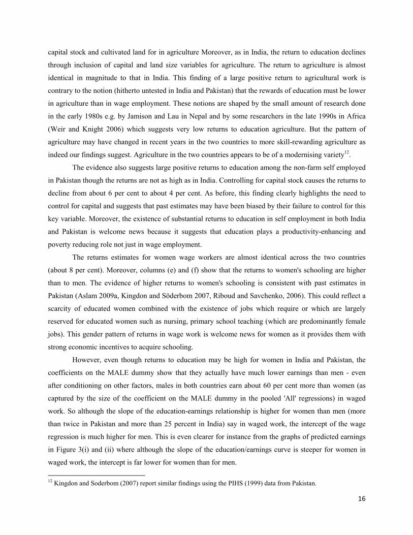
The returns estimates for women wage workers are almost identical across the two countries

(about 8 per cent). Moreover, columns (e) and (f) show that the returns to women's schooling are higher

than to men. The evidence of higher returns to women's schooling is consistent with past estimates in

Pakistan (Aslam 2009a, Kingdon and Söderbom 2007, Riboud and Savchenko, 2006). This could reflect a

scarcity of educated women combined with the existence of jobs which require or which are largely

reserved for educated women such as nursing, primary school teaching (which are predominantly female

jobs). This gender pattern of returns in wage work is welcome news for women as it provides them with

strong economic incentives to acquire schooling.

However, even though returns to education may be high for women in India and Pakistan, the

coefficients on the MALE dummy show that they actually have much lower earnings than men - even

after conditioning on other factors, males in both countries earn about 60 per cent more than women (as

captured by the size of the coefficient on the MALE dummy in the pooled 'All' regressions) in waged

work. So although the slope of the education-earnings relationship is higher for women than men (more

than twice in Pakistan and more than 25 percent in India) say in waged work, the intercept of the wage

regression is much higher for men. This is even clearer for instance from the graphs of predicted earnings

in Figure 3(i) and (ii) where although the slope of the education/earnings curve is steeper for women in

waged work, the intercept is far lower for women than for men.

12 Kingdon and Soderbom (2007) report similar findings using the PIHS (1999) data from Pakistan.

17

As Aslam (2009a) shows, a large part of the gender gap in earnings in Pakistan is not explained by

differences in men's and women's productivity endowments such as education and experience but is due to

potential discrimination in the labour market. However, education of women helps to reduce that earnings

gap. Thus, although women earn less than men and particularly so at low levels of education, at higher

levels of education women’s earnings are almost equal to the men’s as seen in Figure 3(i) and (ii).

Table 4a extends Table 4 for wage workers to distinguish between any possible differential effects

of regular versus casual work. A regular worker dummy interacted with years of education and regular

dummy are introduced as additional variables. In India, introduction of the interaction term drastically

reduces the coefficient of education for all regressions. The coefficient on 'REGULAR' for males suggests

that wage premium to being in a regular job is 15.6% for men with no education. No such effect is

observed for Pakistan. The findings suggest that unlike in Pakistan, the labour market for wage workers in

India is very different for regular and casual wage workers, both males and females. It also suggests that

earnings are not very sensitive to the level of education for casual wage workers. A study (Dutta, 2006)

based on large National Sample Survey Organization (NSSO) samples for 1983, 1993-4 and 1999-2000

also observes that human capital characteristics are not significant determinants of earnings of casual

workers.

Table 5 extends the baseline estimates by including hours worked. This is particularly useful for

agriculture and self employment as degree of involvement of unpaid family labour may vary across

households. In some cases, productivity of unpaid labour may be quite low as they are under employed in

the absence of other productive work opportunities. We find that while introduction of work intensity in

the regressions doesn’t affect the estimates of returns to education, except for non-farm self employed in

India, it does explain a part of variations in earnings in all three occupations in both countries. Agriculture

in India and in Pakistan is one sector where underemployment is quite prevalent. Therefore average work

intensity in agriculture to some extent captures degree of under employment. For the self employed in

India, the coefficient of intensity is significant and high as hours of work do matter for own account

workers which constitute a big portion of the non-farm self employed. For wage work in India, one hour

of additional work per day raises annual earnings by 7.1, 9.9 and 7.6 percent for males, females and all

wage workers respectively. Thus, in India, the effect of work intensity on earnings is somewhat higher for

female wage workers. This could be because the incidence of part time work is usually higher for women

and average wages in such jobs are likely to be low. In Pakistan, the size of intensity is small though we

do note that each hour worked matters more to agricultural work than to self employment or wage work.

18

Extensions on the Education-Earnings Relationship

Correcting for Endogeneity

As stated in Section 2, OLS estimates of returns to education potentially suffer from sample

selectivity and endogeneity biases. We attempted to address the former by employing the Heckman two-

step procedure (explained in Section 2). The underlying MNL regressions on which the graphical analysis

is based were used to calculate the selectivity terms. In all instances, the selectivity-corrected term was not

significant suggesting that sample selection is not a critical problem for agricultural workers, self

employed or wage workers represented in this sample in both India and in Pakistan. Due to space

constraints we do not present any of the sample-selectivity-corrected results nor discuss them further.

As discussed in Section 2, endogeneity bias can also substantially bias estimates of returns to

education. While there are several approaches available in the literature, in this paper we used only one

(discussed below) largely because the objective of this study is to provide a more 'descriptive' bound to the

pattern of returns to different occupations rather than attempt causal estimates. We approached

endogeneity bias by estimating household fixed-effects earnings functions for wage workers. The results

in Table 6 report the fixed-effects estimates. Comparing the coefficient on education in column (g) for 'all'

wage workers in Table 4, we find that while the returns to education fall marginally in both countries

(from about 6.8 per-5.4 per cent in India and from 4.4 per cent to 3.3 per cent in Pakistan). This suggests

the existence of some ability bias.

The household fixed-effects approach is a powerful way to address endogeneity since the

identification of the effect of education on earnings is only due to within-family variation among members

in earnings and in education, and as such it nets out the effect of shared ability in a way similar to the

twin-differencing approach. The fact that the household fixed-effects estimates are not very different from

our baseline OLS estimates gives us confidence in interpreting the OLS estimates.

Shape of the Education-Earnings relationship

So far we have imposed a linear relationship between years of schooling and earnings. This is a

restrictive model as it assumes that the return to each additional year of schooling is the same across each

year. Table 7 relaxes the implicit presumption of linearity by introducing a quadratic term for education.

In India, the education term becomes insignificant in all types of employment, except agriculture where it

has a negative sign, and the quadratic term becomes significant for all occupations. This indicates a

convex education-earnings relationship exists for all occupations in India. The picture is different in

Pakistan. While the education-earnings relationship is definitely quadratic for agricultural self employed,

the relationship appears to be linear for wage workers and the self employed. This finding is inconsistent

19

with recent work in Pakistan (Aslam 2009a). One explanation is that the education-earnings relationship

may be cubic rather than linear. While the results are not reported, when a cubic education term is

introduced, we find that indeed the education-earnings profile is cubic for wage workers and for the self

employed. These findings are consistent with recent work in Pakistan (Aslam 2009a and Kingdon and

Söderbom 2007) and in other developing countries which challenge the previous notion of concave returns

to education and have some critical policy implications (Colclough, Kingdon and Patrinos 2009).

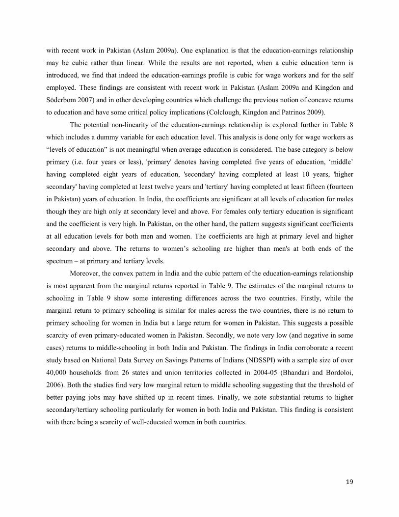
The potential non-linearity of the education-earnings relationship is explored further in Table 8

which includes a dummy variable for each education level. This analysis is done only for wage workers as

“levels of education” is not meaningful when average education is considered. The base category is below

primary (i.e. four years or less), 'primary' denotes having completed five years of education, ‘middle’

having completed eight years of education, 'secondary' having completed at least 10 years, 'higher

secondary' having completed at least twelve years and 'tertiary' having completed at least fifteen (fourteen

in Pakistan) years of education. In India, the coefficients are significant at all levels of education for males

though they are high only at secondary level and above. For females only tertiary education is significant

and the coefficient is very high. In Pakistan, on the other hand, the pattern suggests significant coefficients

at all education levels for both men and women. The coefficients are high at primary level and higher

secondary and above. The returns to women’s schooling are higher than men's at both ends of the

spectrum – at primary and tertiary levels.

Moreover, the convex pattern in India and the cubic pattern of the education-earnings relationship

is most apparent from the marginal returns reported in Table 9. The estimates of the marginal returns to

schooling in Table 9 show some interesting differences across the two countries. Firstly, while the

marginal return to primary schooling is similar for males across the two countries, there is no return to

primary schooling for women in India but a large return for women in Pakistan. This suggests a possible

scarcity of even primary-educated women in Pakistan. Secondly, we note very low (and negative in some

cases) returns to middle-schooling in both India and Pakistan. The findings in India corroborate a recent

study based on National Data Survey on Savings Patterns of Indians (NDSSPI) with a sample size of over

40,000 households from 26 states and union territories collected in 2004-05 (Bhandari and Bordoloi,

2006). Both the studies find very low marginal return to middle schooling suggesting that the threshold of

better paying jobs may have shifted up in recent times. Finally, we note substantial returns to higher

secondary/tertiary schooling particularly for women in both India and Pakistan. This finding is consistent

with there being a scarcity of well-educated women in both countries.

20

4.3 Cognitive Skills, English Language and Earnings

It has been persuasively argued that the 'quality' of schooling matters more than the 'quantity' of

schooling acquired. The estimates so far are based on returns to the 'quantity' of schooling a person has

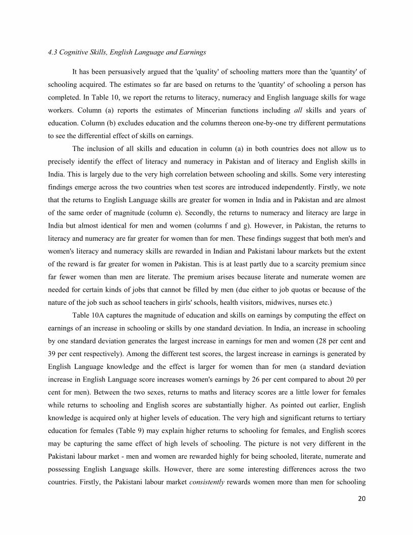
completed. In Table 10, we report the returns to literacy, numeracy and English language skills for wage

workers. Column (a) reports the estimates of Mincerian functions including all skills and years of

education. Column (b) excludes education and the columns thereon one-by-one try different permutations

to see the differential effect of skills on earnings.

The inclusion of all skills and education in column (a) in both countries does not allow us to

precisely identify the effect of literacy and numeracy in Pakistan and of literacy and English skills in

India. This is largely due to the very high correlation between schooling and skills. Some very interesting

findings emerge across the two countries when test scores are introduced independently. Firstly, we note

that the returns to English Language skills are greater for women in India and in Pakistan and are almost

of the same order of magnitude (column e). Secondly, the returns to numeracy and literacy are large in

India but almost identical for men and women (columns f and g). However, in Pakistan, the returns to

literacy and numeracy are far greater for women than for men. These findings suggest that both men's and

women's literacy and numeracy skills are rewarded in Indian and Pakistani labour markets but the extent

of the reward is far greater for women in Pakistan. This is at least partly due to a scarcity premium since

far fewer women than men are literate. The premium arises because literate and numerate women are

needed for certain kinds of jobs that cannot be filled by men (due either to job quotas or because of the

nature of the job such as school teachers in girls' schools, health visitors, midwives, nurses etc.)

Table 10A captures the magnitude of education and skills on earnings by computing the effect on

earnings of an increase in schooling or skills by one standard deviation. In India, an increase in schooling

by one standard deviation generates the largest increase in earnings for men and women (28 per cent and

39 per cent respectively). Among the different test scores, the largest increase in earnings is generated by

English Language knowledge and the effect is larger for women than for men (a standard deviation

increase in English Language score increases women's earnings by 26 per cent compared to about 20 per

cent for men). Between the two sexes, returns to maths and literacy scores are a little lower for females

while returns to schooling and English scores are substantially higher. As pointed out earlier, English

knowledge is acquired only at higher levels of education. The very high and significant returns to tertiary

education for females (Table 9) may explain higher returns to schooling for females, and English scores

may be capturing the same effect of high levels of schooling. The picture is not very different in the

Pakistani labour market - men and women are rewarded highly for being schooled, literate, numerate and

possessing English Language skills. However, there are some interesting differences across the two

countries. Firstly, the Pakistani labour market consistently rewards women more than men for schooling

21

and skills. Secondly, for both men and women in Pakistan, highest rewards accrue from schooling,

followed closely by literacy for both genders. Finally, a standard deviation increase in English Language

skills increases women's earnings by 32 per cent and men's earnings by far less but by a substantial 13 per

cent. Possession of English Language skills seems to be rewarded among Indian men far more than their

Pakistani counterparts and this could have something to do with the types of jobs available. Summarising,

both men's and women's schooling, literacy and English language skills are very highly rewarded in wage

work in India and Pakistan. The Pakistani labour market in particular appears to reward women

substantially for being educated, literate, having knowledge of English and for being numerate. It could be

that English scores are capturing some aspects of the 'quality' of schooling attended and women from

better quality schools engage in more rewarding wage activities compared to women from poorer quality

schools.

5. Conclusions

This study has focussed on some very topical issues regarding the education-earnings relationship

in India and Pakistan in recent years. It has sought to examine (a) the role of education in occupational

attainment; (b) the role of education in raising earnings conditional on occupation; (c) the role of cognitive

skills (literacy and numeracy) in both occupational attainment and earnings determination and (d) the role

of English Language skills in determining earnings. The richness and uniqueness of the survey data

allowed us to go beyond earlier studies in these two countries. For instance, we are able to provide

comparative earnings estimates across different occupations (including agriculture and non-farm self-

employment) for both countries. This is useful as wage-labour is a shrinking part of labour markets across

the developing world. We are also able to control for key variables (such as hours worked, capital stock

and cultivated-land size) that allow a more consistent and nuanced estimation of earnings functions.

Finally, our data allow us to estimate and compare the returns to schooling and skills - literacy, numeracy

and English Language for wage workers that adds a new dimension to an earnings analysis.

The labour market benefits of education accrue both from education promoting a person's entry

into the lucrative occupations and, conditional on occupation, by raising earnings. We find that though

education is seen to be an important determinant of occupation, its effect differs for males and females,

and for urban and rural areas. In India, for males in rural areas, the educated are more likely to move out

of casual work and agriculture, and go for non-farm self employment and regular work. Unexpectedly, the

likelihood of being an unpaid family worker or out of labour force also increases with education. This and

the fact that chances of being in regular work stagnate at higher levels of education suggest unavailability

of suitable jobs for the better educated in rural areas. This phenomenon is not seen in urban areas – the

educated are able to access decent regular work. The trend of the educated being in more lucrative

22

occupation is much clearer. The majority of female workers in rural areas are unpaid family worker or

casual wage earners. With education there is a high likelihood of them withdrawing from the labour force.

In urban areas work participation among females are low and does not vary much with education.

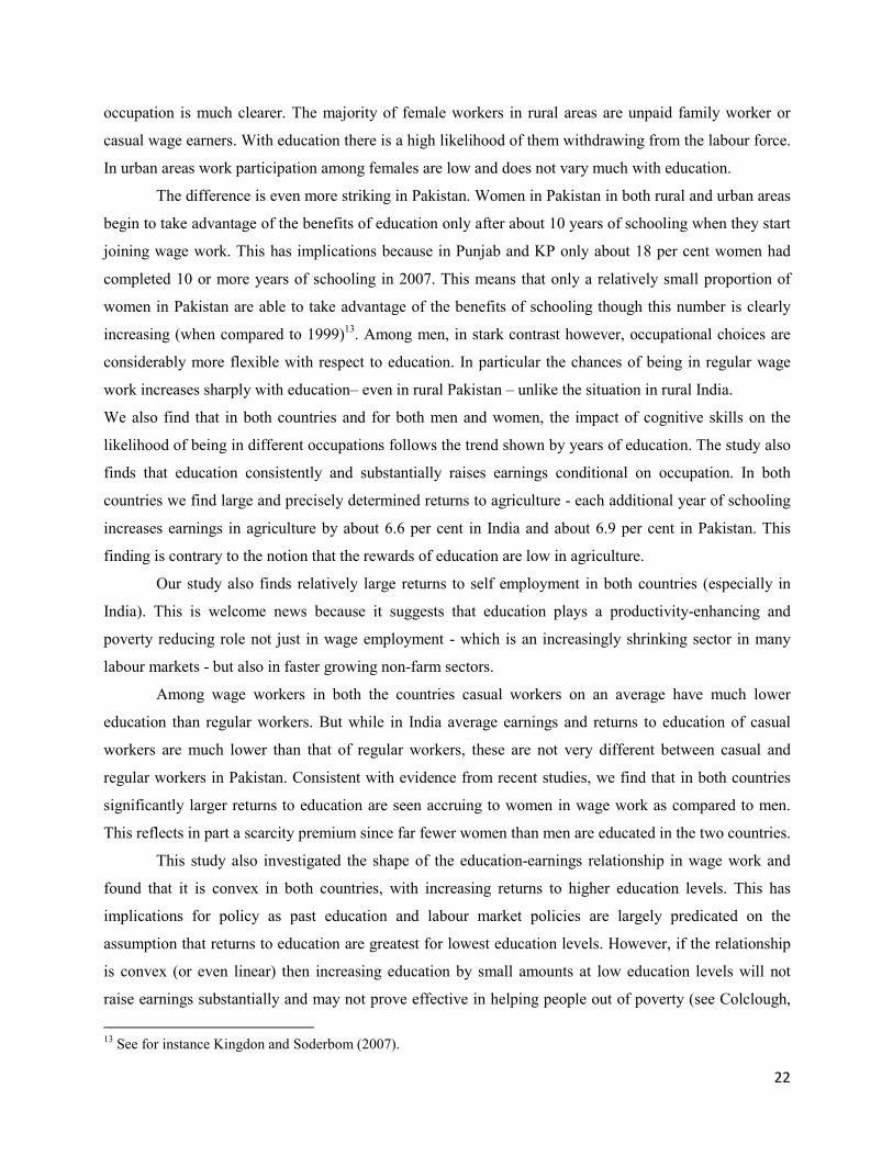
The difference is even more striking in Pakistan. Women in Pakistan in both rural and urban areas

begin to take advantage of the benefits of education only after about 10 years of schooling when they start

joining wage work. This has implications because in Punjab and KP only about 18 per cent women had

completed 10 or more years of schooling in 2007. This means that only a relatively small proportion of

women in Pakistan are able to take advantage of the benefits of schooling though this number is clearly

increasing (when compared to 1999)13. Among men, in stark contrast however, occupational choices are

considerably more flexible with respect to education. In particular the chances of being in regular wage

work increases sharply with education– even in rural Pakistan – unlike the situation in rural India.

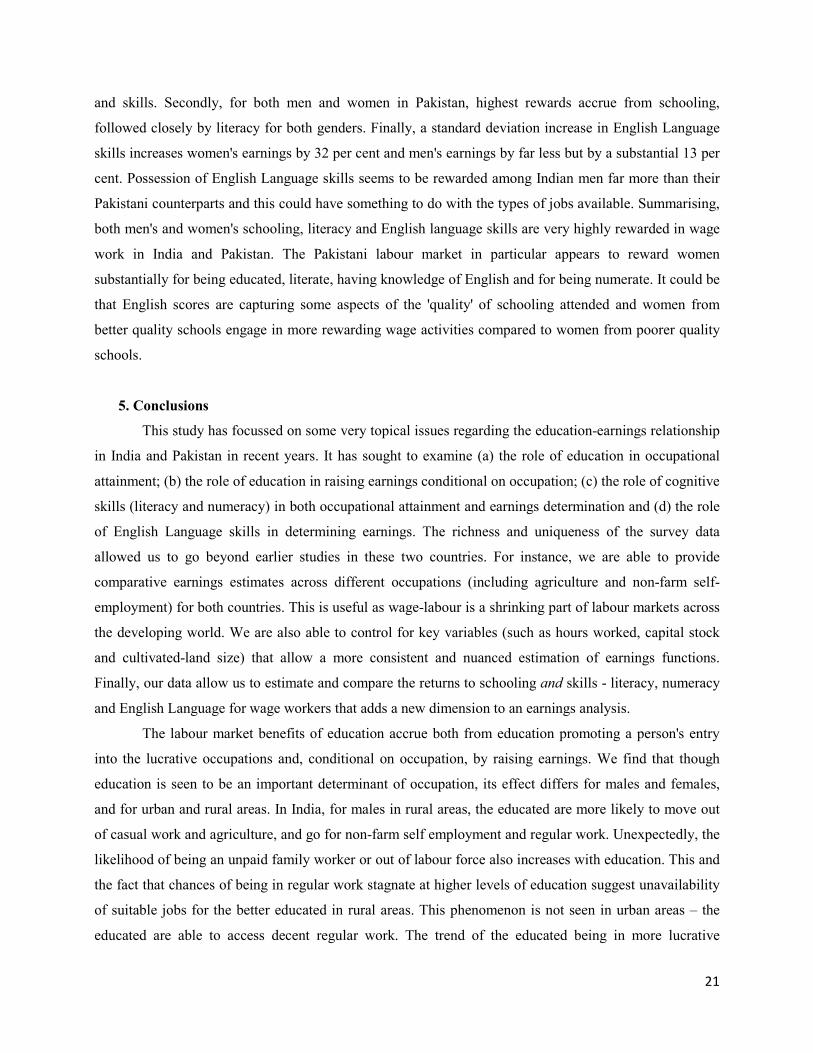
We also find that in both countries and for both men and women, the impact of cognitive skills on the

likelihood of being in different occupations follows the trend shown by years of education. The study also

finds that education consistently and substantially raises earnings conditional on occupation. In both

countries we find large and precisely determined returns to agriculture - each additional year of schooling

increases earnings in agriculture by about 6.6 per cent in India and about 6.9 per cent in Pakistan. This

finding is contrary to the notion that the rewards of education are low in agriculture.

Our study also finds relatively large returns to self employment in both countries (especially in

India). This is welcome news because it suggests that education plays a productivity-enhancing and

poverty reducing role not just in wage employment - which is an increasingly shrinking sector in many

labour markets - but also in faster growing non-farm sectors.

Among wage workers in both the countries casual workers on an average have much lower

education than regular workers. But while in India average earnings and returns to education of casual

workers are much lower than that of regular workers, these are not very different between casual and

regular workers in Pakistan. Consistent with evidence from recent studies, we find that in both countries

significantly larger returns to education are seen accruing to women in wage work as compared to men.

This reflects in part a scarcity premium since far fewer women than men are educated in the two countries.

This study also investigated the shape of the education-earnings relationship in wage work and

found that it is convex in both countries, with increasing returns to higher education levels. This has

implications for policy as past education and labour market policies are largely predicated on the

assumption that returns to education are greatest for lowest education levels. However, if the relationship

is convex (or even linear) then increasing education by small amounts at low education levels will not

raise earnings substantially and may not prove effective in helping people out of poverty (see Colclough,

13 See for instance Kingdon and Soderbom (2007).

23

Kingdon and Patrinos). In Pakistan the returns are high at primary level and then again from higher

secondary level onwards. In India the returns are very high at tertiary level for both males and females. In

both countries the gender gaps in earnings diminish at higher levels of education. From a policy

perspective, women acquiring education above secondary level not only has the potential of raising their

earnings but also to take it to a level similar to men.

Finally, this study has compared returns to years of schooling and to numeracy, literacy and

English Language skills for wage workers. We find that years of schooling are most well rewarded for

men and women in wage work in India followed closely by English Language knowledge. The fact that

schooling is so well rewarded compared to literacy and numeracy skills may suggest some credentialism

in the Indian labour market. Also, very close correspondence between returns to years of schooling and

English knowledge indicates that very high returns at tertiary level of education may be getting reflected

in English knowledge as unlike our literacy and numeracy tests which are at a basic level, English

knowledge is acquired at relatively higher levels of schooling. In Pakistan we find larger rewards to

literacy and numeracy but also substantial rewards to schooling. In particular, the rewards to women's

schooling, and cognitive skills are always far greater than for men in Pakistan.

This study has addressed some highly pertinent issues for India and Pakistan. It has found that

both education and skills promote entry into more lucrative occupations and increase earnings among

workers in different occupations in both countries. It also notes large premiums to education and skills

particularly among women in both countries. However, the constraints imposed by similar conservative

cultures are most apparent in labour market outcomes and these constraints are even more apparent in

Pakistan than they are in India.

24

References

Aslam, M. (2006). Gender and Education in Pakistan, Unpublished DPhil. thesis, University of Oxford. Aslam, M. & Kingdon, G. (2010). Can Education be a Path to Gender Equality in the Labour Market? An

Update on Pakistan, University of Oxford (Mimeo). Aslam, M., De, A., Kingdon, G. & Kumar, R. (2010). Economic Returns to Schooling and Skills – An

Analysis of Pakistan, Working Paper Version, University of Oxford (Mimeo). Aslam, M., Bari, F. & Kingdon, G. (2008). Returns to Schooling, Ability and Skills in Pakistan,

RECOUP Working Paper 20. Aslam, M., Kingdon, G. & Söderbom, M. (2008). Is Female Education a Pathway to Gender Equality in

the Labor Market? Some Evidence from Pakistan. In Tembon, M. (eds) Girls’ Education in the 21st Century: Gender Equality, Empowerment and Growth, The World Bank.

Aslam, M. (2009a). Education Gender Gaps in Pakistan: Is the Labour Market to Blame? Economic

Development and Cultural Change, 57 (4), 747-784. Aslam, M. (2009b) .The Relative Effectiveness of Public and Private Schools in Pakistan: Are Girls

Worse Off? Education Economics, 17 (3), 329-354. Azam, M., Chin, A. & Prakash, N. (2010). The Returns to English Language Skills in India, Centre for

Research and Analysis of Migration Discussion Paper Series, CDP No. 02/10, Department of Economics, University College London.

Bhandari, L. & Bordoloi, M. (2006). Income Differentials and Returns to Education, Economic and

Political Weekly September 9, 2006, 3893-3900. Colclough, C., Kingdon, G. & Patrinos, H. (2009). The Pattern of Returns to Education and its

Implications, Policy Brief No. 4, Centre for Education and International Development, University of Cambridge.

Duraisamy, P. (2002). Changes in the returns to education in India, 1983–94: by gender, age-cohort and

location, Economics of Education Review, 21(6), 609–622. Dutta, P. V. (2006). Returns to Education: New Evidence for India, 1983-1999, Education Economics, 14

(4), 431–451. Hanushek, E.A. & Woessmann, L. (2007), The Role of School Improvement in Economic Development,

Working Paper PEPG 07-01, Program of Education Policy and Governance, Kennedy School of Government, Harvard University.

Hanushek, E.A. (2005). The Economics of School Quality, German Economic Review, 6 (3), 269-286. Heckman, J. (1979). Sample Selection Bias as a Specification Error, Econometrica 47 (1), 153-61. Jamison, D.T. & Lau, L. (1982). Farmer Education and Farm Efficiency, Baltimore: Johns Hopkins.

25

Kingdon, G.G. & Söderbom, M. (2007). Education, Skills and Labor Market Outcomes: Evidence from Pakistan, University of Oxford (Mimeo).

Kingdon, G. G. (1998). Does the Labour Market Explain Lower Female Schooling in India? Journal of

Development Studies, 35 (1), 39-65. Riboud, M., Savchenko, Y. & Tan, H. (2006). The Knowledge Economy and Education and Training in

South Asia: A Mapping Exercise of Available Survey Data, World Bank Working Paper, South Asia Region.

Weir, S. and Knight, J. (2006). Production Externalities of Education: Evidence from Rural Ethiopia,

Journal of African Economies, 16, 134-165.

26

FIGURES

Figure 1: INDIA - Estimated probability of occupation and education

(i) Rural Males

0.1

.2.3

.4Pro

b. o

f Occ

upat

ion

- Rur

al M

ales

0 5 10 15 20highest grade completed in general education

OLF UnemployedUnpaid Family Lab Agri-Self EmpNon-Agri Self Emp Casual WageRegular Wage

(ii) Rural Females

0.2

.4.6

Pro

b. o

f Occ

upat

ion

- Rur

al F

emal

es

0 5 10 15 20highest grade completed in general education

OLF UnemployedUnpaid Family Lab Agri-Self EmpNon-Agri Self Emp Casual WageRegular Wage

27

(iii) Urban Males

0.1

.2.3

.4.5

Pro

b. o

f Occ

upat

ion

- Urb

an M

ales

0 5 10 15 20highest grade completed in general education

OLF UnemployedUnpaid Family Lab Non-Agri Self EmpCasual Wage Regular Wage

(iv) Urban Females

0.2

.4.6

.8Pro

b. o

f Occ

upat

ion

- Urb

an F

emal

es

0 5 10 15 20highest grade completed in general education

OLF UnemployedUnpaid Family Lab Non-Agri Self EmpCasual Wage Regular Wage

28

Figure 2: PAKISTAN - Estimated probability of occupation and education

(i) Rural Males 0

.2.4

.6.8

prob

ability of o

ccup

ation - Rural M

ales

0 5 10 15 20highest grade completed in general education

OLF UnemployedUnpaid Fam Lab Agri-Self EmpNon-Agri Self Emp Casual Wage WorkerRegular Wage Worker

(ii) Rural Females

0.2

.4.6

.8pr

obab

ility

of o

ccup

atio

n - Rur

al F

emal

es

0 5 10 15 20highest grade completed in general education

OLF UnemployedUnpaid Fam Lab Agri-Self EmpNon-Agri Self Emp Casual Wage WorkerRegular Wage Worker

29

(iii) Urban Males

0.2

.4.6

.8pr

obab

ility

of o

ccup

atio

n - Urb

an M

ales

0 5 10 15 20highest grade completed in general education

OLF UnemployedUnpaid Fam Lab Non-Agri Self EmpRegular Wage Worker Casual Wage Worker

(iv) Urban Females

0.2

.4.6

.8pr

obab

ility

of o

ccup

atio

n - Urb

an F

emal

es

0 5 10 15 20highest grade completed in general education

OLF UnemployedUnpaid Fam Lab Non-Agri Self EmpRegular Wage Worker Casual Wage Worker

30

Figure 3: Predicted Earnings and Level of Education for Wage Workers aged 25 and over

(i) INDIA

8.5

99.

510

10.5

11Pre

dicted

log

earn

ings

0 5 10 15eduyears

male female

(ii) PAKISTAN

77.5

88.5

9

Predicted

log ea

rnings

0 5 10 15eduyears

male female

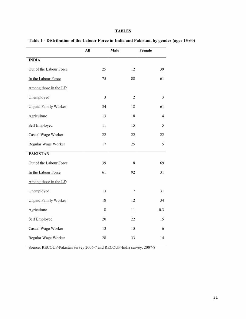
31

TABLES

Table 1 - Distribution of the Labour Force in India and Pakistan, by gender (ages 15-60)

All Male Female

INDIA

Out of the Labour Force 25 12 39

In the Labour Force 75 88 61

Among those in the LF:

Unemployed 3 2 3

Unpaid Family Worker 34 18 61

Agriculture 13 18 4

Self Employed 11 15 5

Casual Wage Worker 22 22 22

Regular Wage Worker 17 25 5

PAKISTAN

Out of the Labour Force 39 8 69

In the Labour Force 61 92 31

Among those in the LF:

Unemployed 13 7 31

Unpaid Family Worker 18 12 34

Agriculture 8 11 0.3

Self Employed 20 22 15

Casual Wage Worker 13 15 6

Regular Wage Worker 28 33 14

Source: RECOUP-Pakistan survey 2006-7 and RECOUP-India survey, 2007-8

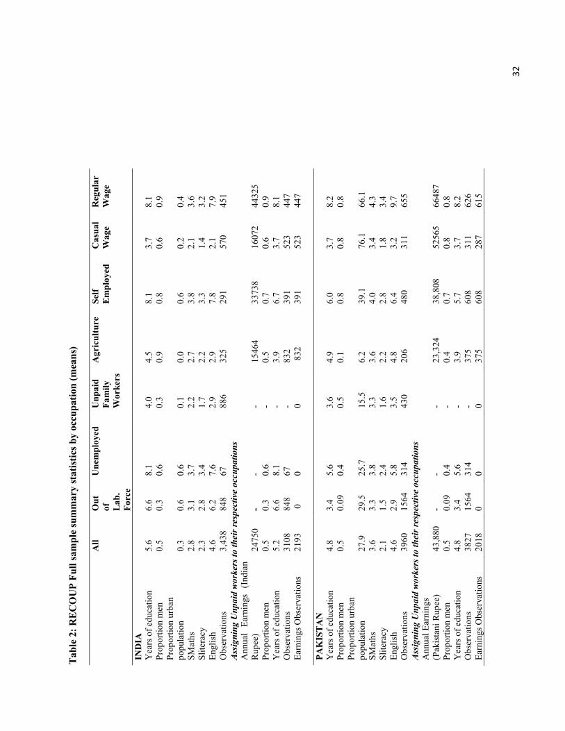
3

2

Tab

le 2: R

ECOUP Full sam

ple summary statistics by occu

pation

(means)

All

Out

of

Lab

. Force

Une

mploy

ed

Unp

aid

Fam

ily

Workers

Agriculture

Self

Employ

ed

Casua

l W

age

Regular

Wag

e

INDIA

Y

ears

of e

duca

tion

5.6

6.6

8.1

4.0

4.5

8.1

3.7

8.1

Prop

ortio

n m

en

0.5

0.3

0.6

0.3

0.9

0.8

0.6

0.9

Prop

ortio

n ur

ban

popu

latio

n 0.

3 0.

6 0.

6 0.

1 0.

0 0.

6 0.

2 0.

4 SM

aths

2.

8 3.

1 3.

7 2.

2 2.

7 3.

8 2.

1 3.

6 Sl

itera

cy

2.3

2.8

3.4

1.7

2.2

3.3

1.4

3.2

Eng

lish

4.6

6.2

7.6

2.9

2.9

7.8

2.1

7.9

Obs

erva

tions

3,

438

848

67

886

325

291

570

451

Assigning Unpaid workers to their respective occupations

A

nnua

l E

arni

ngs

(Ind

ian

Rup

ee)

2475

0 -

- -

1546

4 33

738

1607

2 44

325

Prop

ortio

n m

en

0.5

0.3

0.6

- 0.

5 0.

7 0.

6 0.

9 Y

ears

of e

duca

tion

5.2

6.6

8.1

- 3.

9 6.

7 3.

7 8.

1 O

bser

vatio

ns

3108

84

8 67

-

832

391

523

447

Ear

ning

s O

bser

vatio

ns

2193

0

0

0

8

32

391

52

3 44

7

PAKISTAN

Yea

rs o

f edu

catio

n 4.

8 3.

4 5.

6 3.

6 4.

9 6.

0 3.

7 8.

2 Pr

opor

tion

men

0.

5 0.

09

0.4

0.5

0.1

0.8

0.8

0.8

Prop

ortio

n ur

ban

popu

latio

n 27

.9

29.5

25

.7

15.5

6.

2 39

.1

76.1

66

.1

SMat

hs

3.6

3.3

3.8

3.3

3.6

4.0

3.4

4.3

Slite

racy

2.

1 1.

5 2.

4 1.

6 2.

2 2.

8 1.

8 3.

4 E

nglis

h 4.

6 2.

9 5.

8 3.

5 4.

8 6.

4 3.

2 9.

7 O

bser

vatio

ns

3960

15

64

314

430

206

480

311

655

Assigning Unpaid workers to their respective occupations

A

nnua

l Ear

ning

s (P

akis

tani

Rup

ee)

43,8

80

- -

- 23

,324

38

,808

52

565

6648

7 Pr

opor

tion

men

0.

5 0.

09

0.4

- 0.

4 0.

7 0.

8 0.

8 Y

ears

of e

duca

tion

4.8

3.4

5.6

- 3.

9 5.

7 3.

7 8.

2 O

bser

vatio

ns

3827

15

64

314

- 37

5 60

8 31

1 62

6 E

arni

ngs

Obs

erva

tions

20

18

0 0

0 37

5 60

8 28

7 61

5

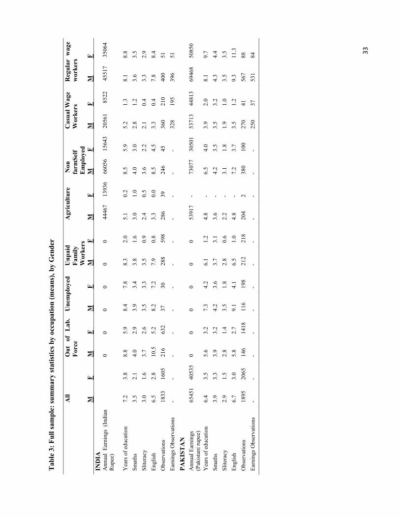
3

3

Tab

le 3: F

ull sam

ple: sum

mary statistics by occu

pation

(means), by

Gen

der

All

Out of Lab

. Force

Une

mploy

ed

Unp

aid

Fam

ily

Workers

Agriculture

Non

farm

Self

Employ

ed

Casua

l Wag

e W

orkers

Regular w

age

workers

M

F

M

F

M

F

M

F

M

F

M

F

M

F

M

F

INDIA

Ann

ual

Ear

ning

s (I

ndia

n R

upee

)

0 0

0 0

0 0

4446

7 13

936

6605

6 15

643

2056

1 85

22

4551

7 35

064

Yea

rs o

f edu

catio

n

7.2

3.8

8.8

5.9

8.4

7.8

8.3

2.0

5.1

0.2

8.5

5.9

5.2

1.3

8.1

8.8

Smat

hs

3.

5 2.

1 4.

0 2.

9 3.

9 3.

4 3.

8 1.

6 3.

0 1.

0 4.

0 3.

0 2.

8 1.

2 3.

6 3.

5

Slite

racy

3.0

1.6

3.7

2.6

3.5

3.3

3.5

0.9

2.4

0.5

3.6

2.2

2.1

0.4

3.3

2.9

Eng

lish

6.

5 2.

8 10

.5

5.2

8.2

7.2

7.9

0.8

3.3

0.0

8.5

4.5

3.3

0.4

7.8

8.4

Obs

erva

tions

18

33

1605

21

6 63

2 37

30

28

8 59

8 28

6 39

24

6 45

36

0 21

0 40

0 51

Ear

ning

s O

bser

vatio

ns

- -

- -

- -

- -

- -

- -

328

195

396

51

PAKISTAN

Ann

ual E

arni

ngs

(Pak

ista

ni ru

pee)

6545

1 40

535

0 0

0 0

0 0

5391

7 -

7307

7 30

501

5371

3 44

813

6946

8 50

850

Yea

rs o

f edu

catio

n

6.4

3.5

5.6

3.2

7.3

4.2

6.1

1.2

4.8

- 6.

5 4.

0 3.

9 2.

0 8.

1 9.

7

Smat

hs

3.

9 3.

3 3.

9 3.

2 4.

2 3.

6 3.

7 3.

1 3.

6 -

4.2

3.5

3.5

3.2

4.3

4.4

Slite

racy

2.9

1.5

2.8

1.4

3.5

1.8

2.8

0.6

2.2

- 3.

1 1.

8 1.

9 1.

0 3.

5 3.

5

Eng

lish

6.

7 3.

0 5.

8 2.

7 9.

1 4.

1 6.

5 1.

0 4.

8 -

7.2

3.7

3.5

1.2

9.3

11.3

Obs

erva

tions

1895

20

65

146

1418

11

6 19

8 21

2 21

8 20

4 2

380

100

270

41

567

88

Ear

ning

s O

bser

vatio

ns

-

- -

- -

- -

- -

- -

- 25

0 37

53

1 84

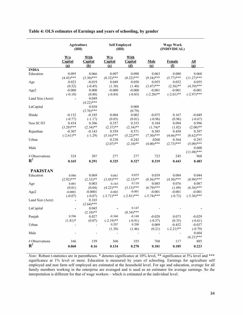
34

Table 4: OLS estimates of Earnings and years of schooling, by gender

Agriculture (HH)

Self Employed

(HH)

Wage Work (INDIVIDUAL)

W/o Capital

(a)

With Capital (b)

W/o Capital

(c)

With Capital (d)

Male (e)

Female (f)

All (g)

INDIA Education 0.095 0.066 0.097 0.098 0.063 0.080 0.068 (4.43)*** (3.30)*** (8.32)*** (8.22)*** (9.34)*** (5.77)*** (11.27)*** Age 0.022 -0.019 0.049 0.050 0.055 0.052 0.055 (0.52) (-0.45) (1.38) (1.40) (3.47)*** (2.56)** (4.39)*** Age2 -0.000 0.000 -0.000 -0.000 -0.001 -0.001 -0.001 (-0.10) (0.88) (-0.84) (-0.85) (-2.20)** (-2.01)** (-2.97)*** Land Size (Acre) - 0.049 (4.22)*** LnCapital 0.038 0.008 (3.76)*** (0.79) Hindu -0.132 -0.185 0.004 0.002 -0.075 0.167 -0.049 (-0.77) (-1.17) (0.03) (0.01) (-0.96) (0.96) (-0.67) Non SC/ST 0.434 0.306 0.357 0.353 0.104 0.094 0.996 (3.29)*** (2.34)** (2.37)** (2.34)** (1.74)* (1.02) (2.00)** Rajasthan -0.307 -0.143 0.559 0.571 0.385 0.450 0.397 (-2.61)** (-1.29) (5.16)*** (5.22)*** (7.30)*** (4.66)*** (8.62)*** Urban 0.238 0.242 .0260 0.364 0.293 (2.07)** (2.10)** (4.00)*** (2.73)*** (5.09)*** Male 0.600 (11.08)*** # Observations 324 307 277 277 723 245 968 R2 0.165 0.291 0.325 0.327 0.319 0.443 0.483 PAKISTAN

Education 0.086 0.069 0.061 0.035 0.039 0.084 0.044 (2.92)*** (2.33)** (3.45)*** (2.15)** (8.56)*** (4.30)*** (8.99)*** Age 0.001 0.003 0.165 0.110 0.085 0.076 0.087 (0.01) (0.04) (4.22)*** (3.13)*** (6.79)*** (1.09) (6.36)*** Age2 -0.0001 -0.0001 -0.002 -0.001 -0.001 -0.001 -0.001 (-0.07) (-0.07) (-3.71)*** (-2.81)*** (-5.74)*** (-0.73) (-5.36)*** Land Size (Acre) - 0.103 (2.64)*** LnCapital - 0.045 - 0.147 - - - (2.10)** (8.34)*** Punjab 0.596 0.027 -0.360 -0.148 -0.028 0.073 -0.029 (1.81)* (0.07) (-2.19)** (-0.91) (-0.57) (0.35) (-0.61) Urban - - 0.207 0.200 0.009 -0.452 -0.037 (1.38) (1.46) (0.21) (-2.21)** (-0.79) Male - - - - - - 0.604 (6.21)*** # Observations 166 159 360 355 768 117 885 R2 0.060 0.16 0.134 0.270 0.181 0.185 0.223

Note: Robust t-statistics are in parentheses. * denotes significance at 10% level, ** significance at 5% level and *** significance at 1% level or more. Education is measured by years of schooling. Earnings for agriculture self employed and non farm self employed are estimated at the household level. For age and education, average for all family members working in the enterprise are averaged and is used as an estimator for average earnings. So the interpretation is different for that of wage workers – which is estimated at the individual level.

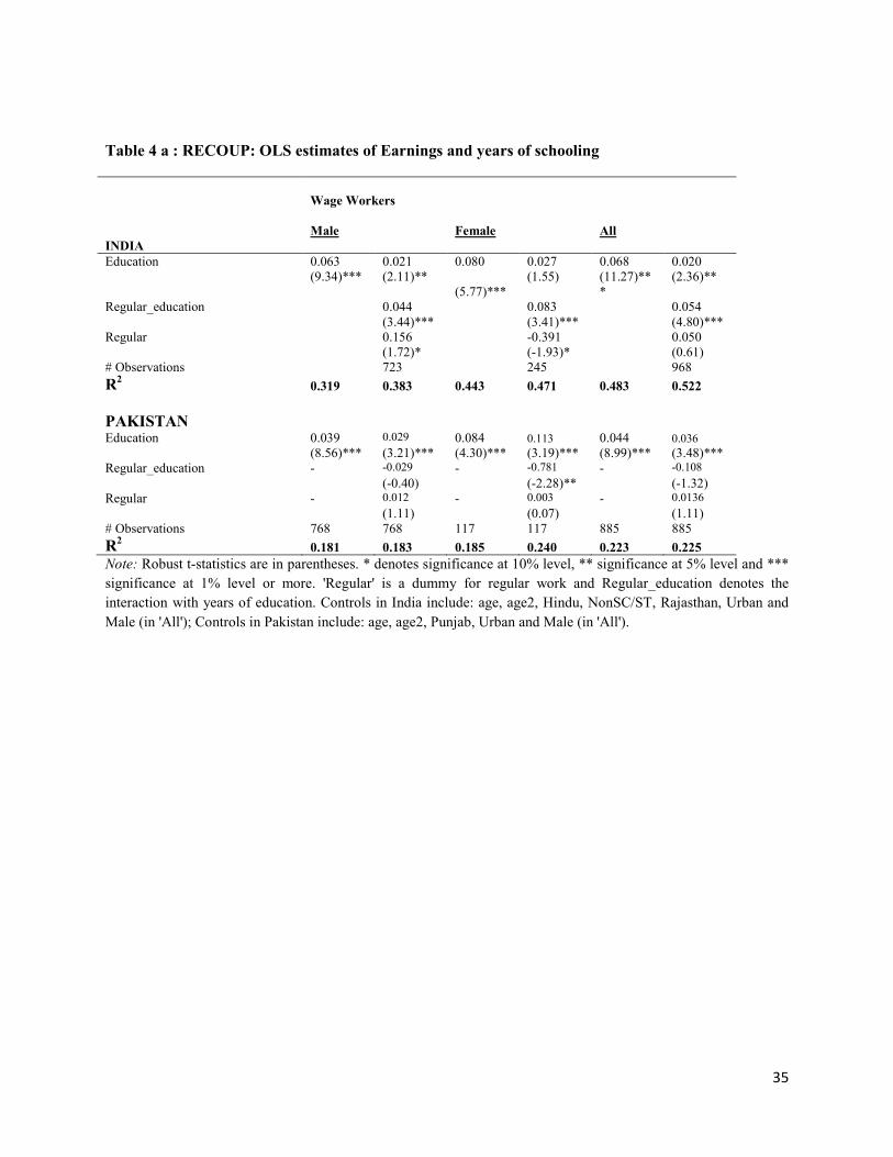
35

Table 4 a : RECOUP: OLS estimates of Earnings and years of schooling

Wage Workers

INDIA Male

Female

All

Education 0.063 0.021 0.080 0.027 0.068 0.020

(9.34)*** (2.11)**

(5.77)*** (1.55) (11.27)**

* (2.36)**

Regular_education 0.044 0.083 0.054 (3.44)*** (3.41)*** (4.80)*** Regular 0.156 -0.391 0.050 (1.72)* (-1.93)* (0.61) # Observations 723 245 968 R2 0.319 0.383 0.443 0.471 0.483 0.522 PAKISTAN Education 0.039 0.029 0.084 0.113 0.044 0.036 (8.56)*** (3.21)*** (4.30)*** (3.19)*** (8.99)*** (3.48)*** Regular_education - -0.029 - -0.781 - -0.108 (-0.40) (-2.28)** (-1.32) Regular - 0.012 - 0.003 - 0.0136 (1.11) (0.07) (1.11) # Observations 768 768 117 117 885 885 R2 0.181 0.183 0.185 0.240 0.223 0.225 Note: Robust t-statistics are in parentheses. * denotes significance at 10% level, ** significance at 5% level and *** significance at 1% level or more. 'Regular' is a dummy for regular work and Regular_education denotes the interaction with years of education. Controls in India include: age, age2, Hindu, NonSC/ST, Rajasthan, Urban and Male (in 'All'); Controls in Pakistan include: age, age2, Punjab, Urban and Male (in 'All').

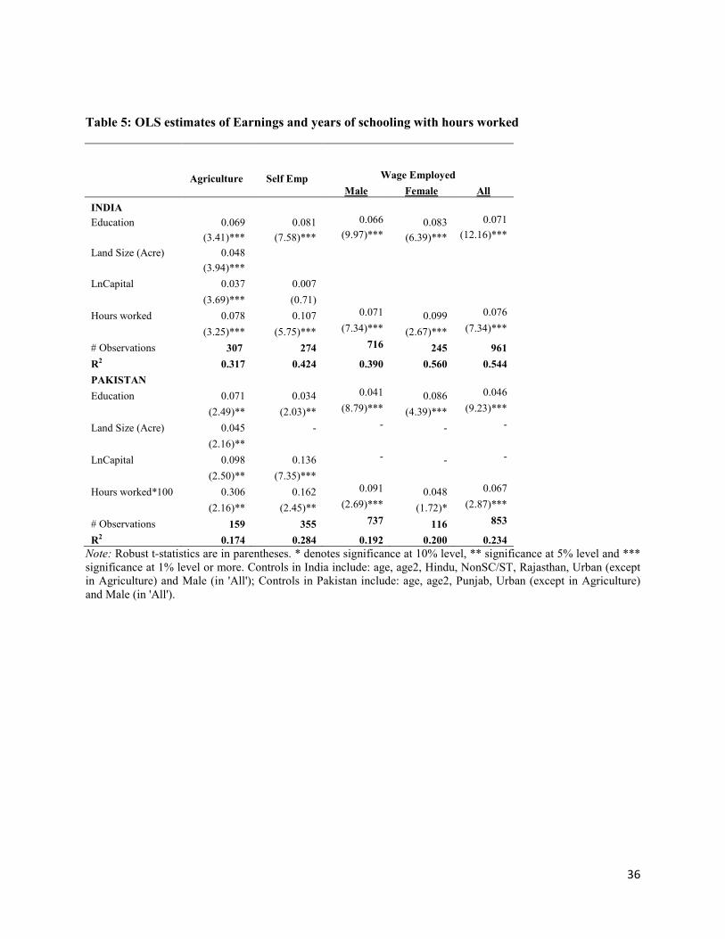
36

Table 5: OLS estimates of Earnings and years of schooling with hours worked

Agriculture

Self Emp

Wage Employed Male Female All

INDIA Education 0.069 0.081 0.066 0.083 0.071

(3.41)*** (7.58)*** (9.97)*** (6.39)*** (12.16)***

Land Size (Acre) 0.048

(3.94)***

LnCapital 0.037 0.007 (3.69)*** (0.71)

Hours worked 0.078 0.107 0.071 0.099 0.076

(3.25)*** (5.75)*** (7.34)*** (2.67)*** (7.34)***

# Observations 307 274 716 245 961

R2 0.317 0.424 0.390 0.560 0.544 PAKISTAN Education 0.071 0.034 0.041 0.086 0.046

(2.49)** (2.03)** (8.79)*** (4.39)*** (9.23)***

Land Size (Acre) 0.045 - - - -

(2.16)**

LnCapital 0.098 0.136 - - -

(2.50)** (7.35)***

Hours worked*100 0.306 0.162 0.091 0.048 0.067

(2.16)** (2.45)** (2.69)*** (1.72)* (2.87)***

# Observations 159 355 737 116 853

R2 0.174 0.284 0.192 0.200 0.234 Note: Robust t-statistics are in parentheses. * denotes significance at 10% level, ** significance at 5% level and *** significance at 1% level or more. Controls in India include: age, age2, Hindu, NonSC/ST, Rajasthan, Urban (except in Agriculture) and Male (in 'All'); Controls in Pakistan include: age, age2, Punjab, Urban (except in Agriculture) and Male (in 'All').

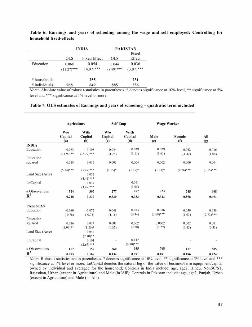
37

Table 6: Earnings and years of schooling among the wage and self employed: Controlling for household fixed-effects

INDIA PAKISTAN

OLS Fixed Effect OLS Fixed Effect

Education 0.068 0.054 0.044 0.036 (11.27)*** (4.97)*** (8.99)*** (3.07)*** # households 255 231 # individuals 968 649 885 536 Note: Absolute value of robust t-statistics in parentheses. * denotes significance at 10% level, ** significance at 5% level and *** significance at 1% level or more.

Table 7: OLS estimates of Earnings and years of schooling – quadratic term included

Agriculture

Self Emp

Wage Worker

W/o Capital

(a)

With Capital (b)

W/o Capital

(c)

With Capital (d)

Male (e)

Female (f)

All (g)

INDIA Education -0.083 -0.108 0.044 0.039 0.029 -0.042 0.016 (-1.99)** (-2.79)*** (1.26) (1.11) (1.61) (-1.42) (1.04) Education squared 0.018 0.017 0.003 0.004 0.002 0.009 0.004

(5.14)*** (5.47)*** (1.65)*

(1.85)*

(1.83)* (4.26)*** (3.15)*** Land Size (Acre) 0.052 (4.41)*** LnCapital 0.034 0.011 (3.49)*** (1.05) # Observations 324 307 277 277 723 245 968 R2 0.216 0.339 0.330 0.333 0.323 0.598 0.491

PAKISTAN Education -0.080 -0.072 0.048 0.013 0.036 0.059 0.038 (-0.78) (-0.74) (1.11) (0.34) (2.69)*** (1.03) (2.73)*** Education squared 0.016 0.014 0.001 0.002 0.0002 0.002 0.001 (1.96)** (1.80)* (0.35) (0.70) (0.29) (0.45) (0.51) Land Size (Acre) 0.044 (2.10)** LnCapital 0.101 - 0.147 - - - (2.67)*** (8.30)*** # Observations 167 159 360 355 768 117 885

R2 0.075 0.168 0.134 0.271 0.181 0.186 0.224 Note: Robust t-statistics are in parentheses. * denotes significance at 10% level, ** significance at 5% level and *** significance at 1% level or more; LnCapital denotes the natural log of the value of business/farm equipment/capital owned by individual and averaged for the household; Controls in India include: age, age2, Hindu, NonSC/ST, Rajasthan, Urban (except in Agriculture) and Male (in 'All'); Controls in Pakistan include: age, age2, Punjab, Urban (except in Agriculture) and Male (in 'All').

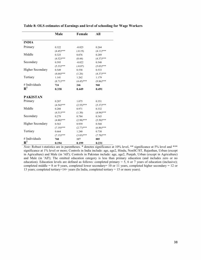
38

Table 8: OLS estimates of Earnings and level of schooling for Wage Workers

Male

Female

All

INDIA

Primary 0.322 -0.025 0.264 (4.45)*** (-0.19) (4.11)*** Middle 0.325 0.076 0.289 (4.52)*** (0.44) (4.37)*** Secondary 0.595 -0.022 0.548 (5.33)*** (-0.07) (5.03)*** Higher Secondary 0.549 0.558 0.533 (4.64)*** (1.26) (4.37)*** Tertiary 1.141 1.262 1.179 (8.71)*** (4.45)*** (9.86)*** # Individuals 724 246 968

R2 0.338 0.449 0.491 PAKISTAN Primary 0.287 1.075 0.351 (4.54)*** (2.55)*** (5.37)*** Middle 0.288 0.971 0.332 (4.51)*** (1.30) (4.94)*** Secondary 0.279 0.784 0.343 (4.80)*** (2.98)*** (5.50)*** Higher Secondary 0.563 0.939 0.568 (7.19)*** (2.77)*** (6.86)*** Tertiary 0.664 1.240 0.730 (7.15)*** (3.83)*** (7.70)*** # Individuals 768 117 885

R2 0.194 0.199 0.231 Note: Robust t-statistics are in parentheses. * denotes significance at 10% level, ** significance at 5% level and *** significance at 1% level or more; Controls in India include: age, age2, Hindu, NonSC/ST, Rajasthan, Urban (except in Agriculture) and Male (in 'All'); Controls in Pakistan include: age, age2, Punjab, Urban (except in Agriculture) and Male (in 'All'); The omitted education category is less than primary education (and includes zero or no education). Education levels are defined as follows: completed primary = 5, 6 or 7 years of education (inclusive); completed middle = 8 or 9 years, completed lower secondary= 10 or 11 years, completed higher secondary = 12 or 13 years; completed tertiary=14+ years (In India, completed tertiary = 15 or more years).

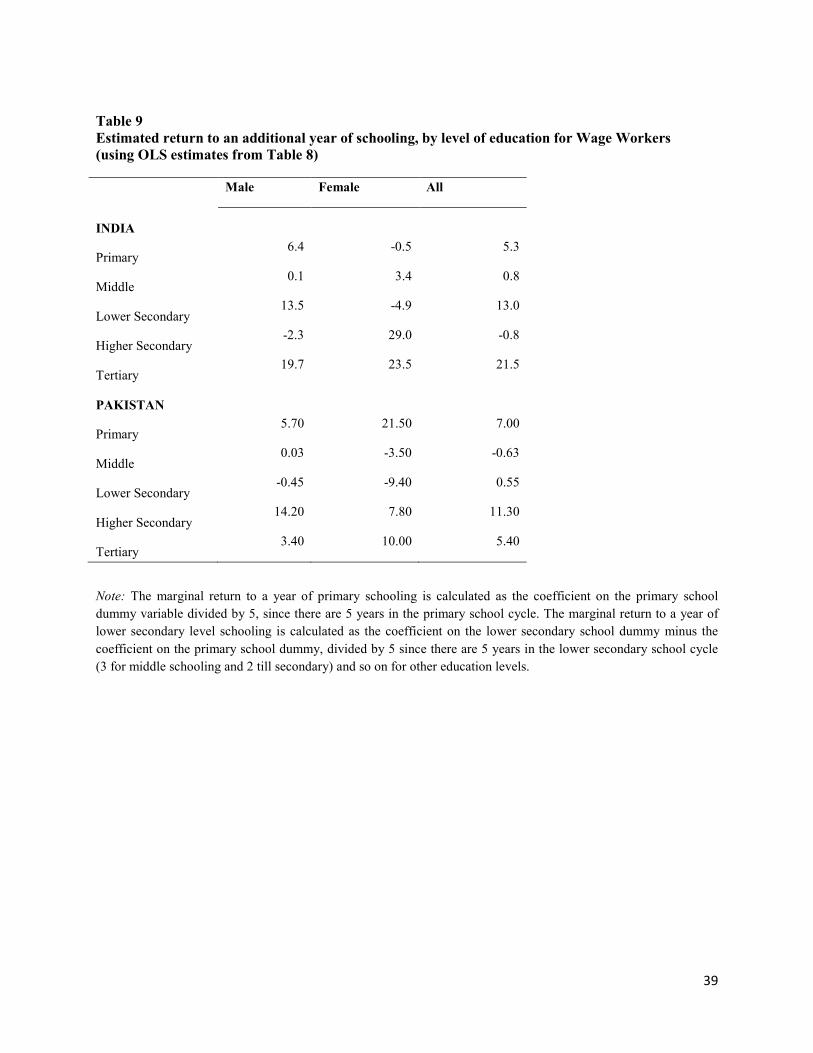
39

Table 9 Estimated return to an additional year of schooling, by level of education for Wage Workers (using OLS estimates from Table 8)

Note: The marginal return to a year of primary schooling is calculated as the coefficient on the primary school dummy variable divided by 5, since there are 5 years in the primary school cycle. The marginal return to a year of lower secondary level schooling is calculated as the coefficient on the lower secondary school dummy minus the coefficient on the primary school dummy, divided by 5 since there are 5 years in the lower secondary school cycle (3 for middle schooling and 2 till secondary) and so on for other education levels.

Male Female All

INDIA

Primary 6.4 -0.5 5.3

Middle 0.1 3.4 0.8

Lower Secondary 13.5 -4.9 13.0

Higher Secondary -2.3 29.0 -0.8

Tertiary 19.7 23.5 21.5

PAKISTAN

Primary 5.70 21.50 7.00

Middle 0.03 -3.50 -0.63

Lower Secondary -0.45 -9.40 0.55

Higher Secondary 14.20 7.80 11.30

Tertiary 3.40 10.00 5.40

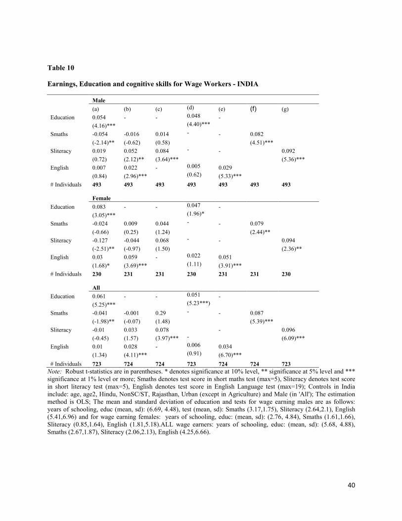
40

Table 10

Earnings, Education and cognitive skills for Wage Workers - INDIA

Male (a) (b) (c) (d) (e) (f) (g) Education 0.054 - - 0.048 - (4.16)*** (4.40)*** Smaths -0.054 -0.016 0.014 - - 0.082 (-2.14)** (-0.62) (0.58) (4.51)*** Sliteracy 0.019 0.052 0.084 - - 0.092 (0.72) (2.12)** (3.64)*** (5.36)*** English 0.007 0.022 - 0.005 0.029 (0.84) (2.96)*** (0.62) (5.33)*** # Individuals 493 493 493 493 493 493 493

Female

Education 0.083 - - 0.047 - (3.05)*** (1.96)* Smaths -0.024 0.009 0.044 - - 0.079 (-0.66) (0.25) (1.24) (2.44)** Sliteracy -0.127 -0.044 0.068 - - 0.094 (-2.51)** (-0.97) (1.50) (2.36)** English 0.03 0.059 - 0.022 0.051 (1.68)* (3.69)*** (1.11) (3.91)*** # Individuals 230 231 231 230 231 231 230

All

Education 0.061 - - 0.051 - (5.25)*** (5.23***) Smaths -0.041 -0.001 0.29 - - 0.087 (-1.98)** (-0.07) (1.48) (5.39)*** Sliteracy -0.01 0.033 0.078 - 0.096 (-0.45) (1.57) (3.97)*** - (6.09)*** English 0.01 0.028 - 0.006 0.034 (1.34) (4.11)*** (0.91) (6.70)***

# Individuals 723 724 724 723 724 724 723 Note: Robust t-statistics are in parentheses. * denotes significance at 10% level, ** significance at 5% level and *** significance at 1% level or more; Smaths denotes test score in short maths test (max=5), Sliteracy denotes test score in short literacy test (max=5), English denotes test score in English Language test (max=19); Controls in India include: age, age2, Hindu, NonSC/ST, Rajasthan, Urban (except in Agriculture) and Male (in 'All'); The estimation method is OLS; The mean and standard deviation of education and tests for wage earning males are as follows: years of schooling, educ (mean, sd): (6.69, 4.48), test (mean, sd): Smaths (3.17,1.75), Sliteracy (2.64,2.1), English (5.41,6.96) and for wage earning females: years of schooling, educ: (mean, sd): (2.76, 4.84), Smaths (1.61,1.66), Sliteracy (0.85,1.64), English (1.81,5.18).ALL wage earners: years of schooling, educ: (mean, sd): (5.68, 4.88), Smaths (2.67,1.87), Sliteracy (2.06,2.13), English (4.25,6.66).

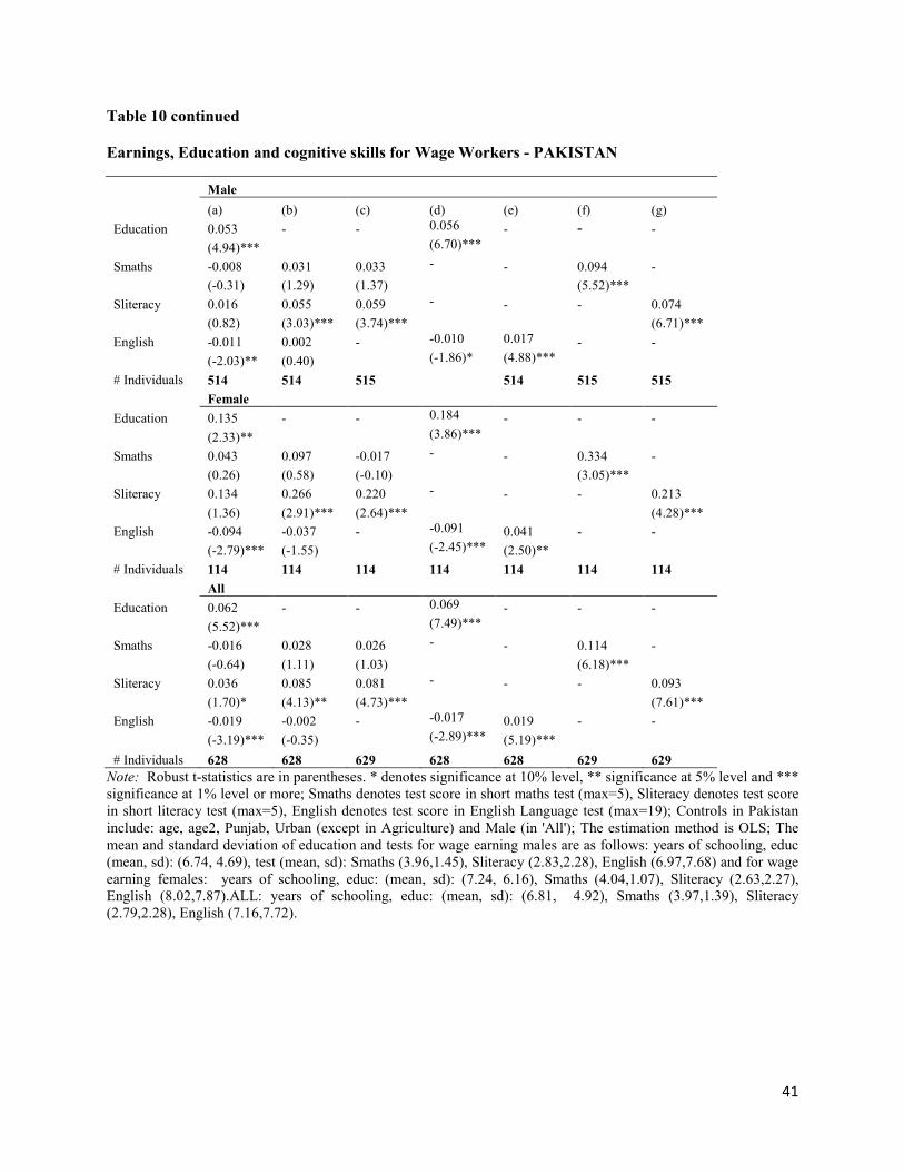
41

Table 10 continued

Earnings, Education and cognitive skills for Wage Workers - PAKISTAN

Male (a) (b) (c) (d) (e) (f) (g)

Education 0.053 - - 0.056 - - - (4.94)*** (6.70)*** Smaths -0.008 0.031 0.033 - - 0.094 - (-0.31) (1.29) (1.37) (5.52)*** Sliteracy 0.016 0.055 0.059 - - - 0.074 (0.82) (3.03)*** (3.74)*** (6.71)*** English -0.011 0.002 - -0.010 0.017 - - (-2.03)** (0.40) (-1.86)* (4.88)*** # Individuals 514 514 515 514 515 515 Female Education 0.135 - - 0.184 - - - (2.33)** (3.86)*** Smaths 0.043 0.097 -0.017 - - 0.334 - (0.26) (0.58) (-0.10) (3.05)*** Sliteracy 0.134 0.266 0.220 - - - 0.213 (1.36) (2.91)*** (2.64)*** (4.28)*** English -0.094 -0.037 - -0.091 0.041 - - (-2.79)*** (-1.55) (-2.45)*** (2.50)** # Individuals 114 114 114 114 114 114 114 All Education 0.062 - - 0.069 - - - (5.52)*** (7.49)*** Smaths -0.016 0.028 0.026 - - 0.114 - (-0.64) (1.11) (1.03) (6.18)*** Sliteracy 0.036 0.085 0.081 - - - 0.093 (1.70)* (4.13)** (4.73)*** (7.61)*** English -0.019 -0.002 - -0.017 0.019 - - (-3.19)*** (-0.35) (-2.89)*** (5.19)*** # Individuals 628 628 629 628 628 629 629 Note: Robust t-statistics are in parentheses. * denotes significance at 10% level, ** significance at 5% level and *** significance at 1% level or more; Smaths denotes test score in short maths test (max=5), Sliteracy denotes test score in short literacy test (max=5), English denotes test score in English Language test (max=19); Controls in Pakistan include: age, age2, Punjab, Urban (except in Agriculture) and Male (in 'All'); The estimation method is OLS; The mean and standard deviation of education and tests for wage earning males are as follows: years of schooling, educ (mean, sd): (6.74, 4.69), test (mean, sd): Smaths (3.96,1.45), Sliteracy (2.83,2.28), English (6.97,7.68) and for wage earning females: years of schooling, educ: (mean, sd): (7.24, 6.16), Smaths (4.04,1.07), Sliteracy (2.63,2.27), English (8.02,7.87).ALL: years of schooling, educ: (mean, sd): (6.81, 4.92), Smaths (3.97,1.39), Sliteracy (2.79,2.28), English (7.16,7.72).

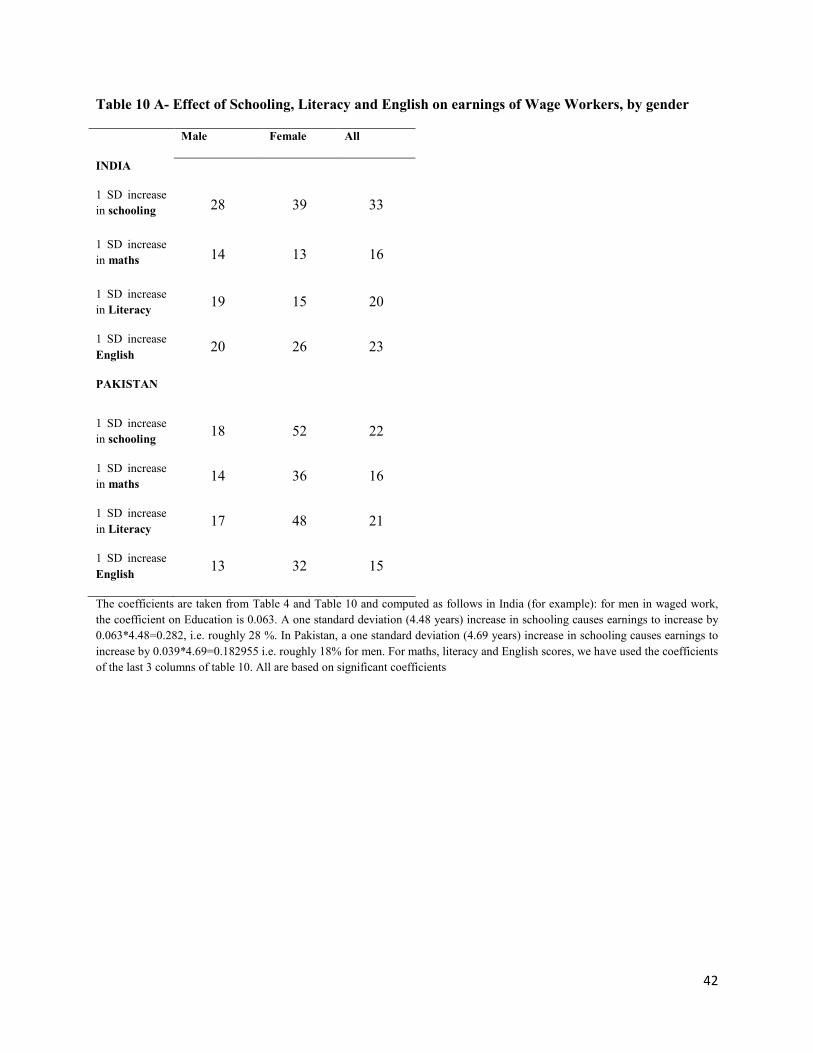
42

Table 10 A- Effect of Schooling, Literacy and English on earnings of Wage Workers, by gender

Male Female All

INDIA

1 SD increase in schooling 28 39 33

1 SD increase in maths 14 13 16

1 SD increase in Literacy

19 15 20

1 SD increase English

20 26 23

PAKISTAN

1 SD increase in schooling

18 52 22

1 SD increase in maths

14 36 16

1 SD increase in Literacy

17 48 21

1 SD increase English

13 32 15

The coefficients are taken from Table 4 and Table 10 and computed as follows in India (for example): for men in waged work, the coefficient on Education is 0.063. A one standard deviation (4.48 years) increase in schooling causes earnings to increase by 0.063*4.48=0.282, i.e. roughly 28 %. In Pakistan, a one standard deviation (4.69 years) increase in schooling causes earnings to increase by 0.039*4.69=0.182955 i.e. roughly 18% for men. For maths, literacy and English scores, we have used the coefficients of the last 3 columns of table 10. All are based on significant coefficients

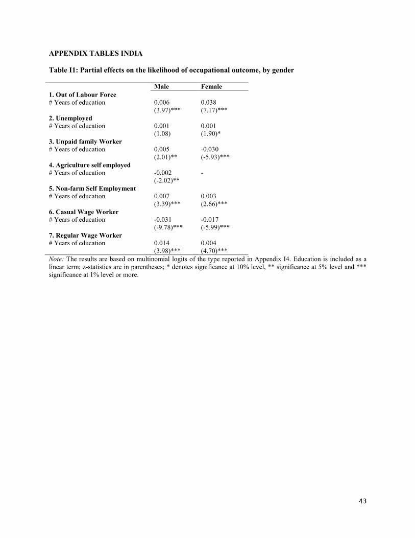
43

APPENDIX TABLES INDIA

Table I1: Partial effects on the likelihood of occupational outcome, by gender

Male Female 1. Out of Labour Force # Years of education 0.006 0.038 (3.97)*** (7.17)*** 2. Unemployed # Years of education 0.001 0.001 (1.08) (1.90)* 3. Unpaid family Worker # Years of education 0.005 -0.030 (2.01)** (-5.93)*** 4. Agriculture self employed # Years of education -0.002 - (-2.02)** 5. Non-farm Self Employment # Years of education 0.007 0.003 (3.39)*** (2.66)*** 6. Casual Wage Worker # Years of education -0.031 -0.017 (-9.78)*** (-5.99)*** 7. Regular Wage Worker # Years of education 0.014 0.004 (3.98)*** (4.70)*** Note: The results are based on multinomial logits of the type reported in Appendix I4. Education is included as a linear term; z-statistics are in parentheses; * denotes significance at 10% level, ** significance at 5% level and *** significance at 1% level or more.

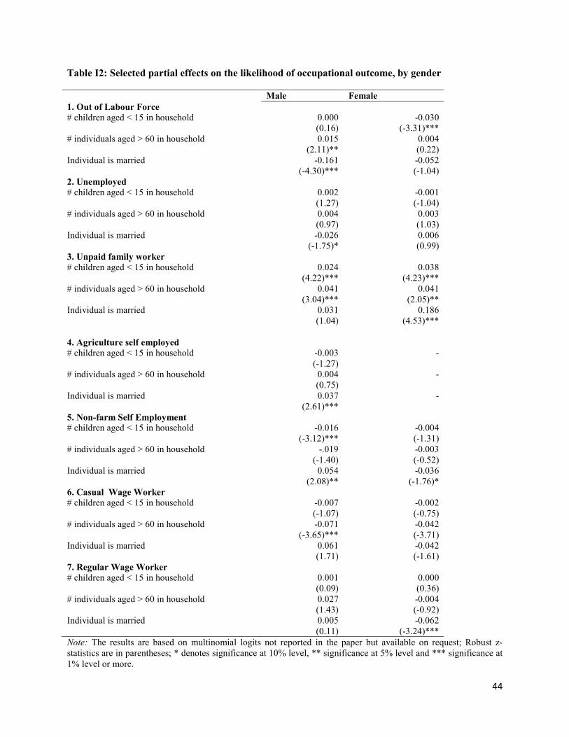
44

Table I2: Selected partial effects on the likelihood of occupational outcome, by gender

Male Female 1. Out of Labour Force # children aged < 15 in household 0.000 -0.030 (0.16) (-3.31)*** # individuals aged > 60 in household 0.015 0.004 (2.11)** (0.22) Individual is married -0.161 -0.052 (-4.30)*** (-1.04) 2. Unemployed # children aged < 15 in household 0.002 -0.001 (1.27) (-1.04) # individuals aged > 60 in household 0.004 0.003 (0.97) (1.03) Individual is married -0.026 0.006 (-1.75)* (0.99) 3. Unpaid family worker # children aged < 15 in household 0.024 0.038 (4.22)*** (4.23)*** # individuals aged > 60 in household 0.041 0.041 (3.04)*** (2.05)** Individual is married 0.031 0.186 (1.04) (4.53)*** 4. Agriculture self employed # children aged < 15 in household -0.003 - (-1.27) # individuals aged > 60 in household 0.004 - (0.75) Individual is married 0.037 - (2.61)*** 5. Non-farm Self Employment # children aged < 15 in household -0.016 -0.004 (-3.12)*** (-1.31) # individuals aged > 60 in household -.019 -0.003 (-1.40) (-0.52) Individual is married 0.054 -0.036 (2.08)** (-1.76)* 6. Casual Wage Worker # children aged < 15 in household -0.007 -0.002 (-1.07) (-0.75) # individuals aged > 60 in household -0.071 -0.042 (-3.65)*** (-3.71) Individual is married 0.061 -0.042 (1.71) (-1.61) 7. Regular Wage Worker # children aged < 15 in household 0.001 0.000 (0.09) (0.36) # individuals aged > 60 in household 0.027 -0.004 (1.43) (-0.92) Individual is married 0.005 -0.062 (0.11) (-3.24)*** Note: The results are based on multinomial logits not reported in the paper but available on request; Robust z-statistics are in parentheses; * denotes significance at 10% level, ** significance at 5% level and *** significance at 1% level or more.

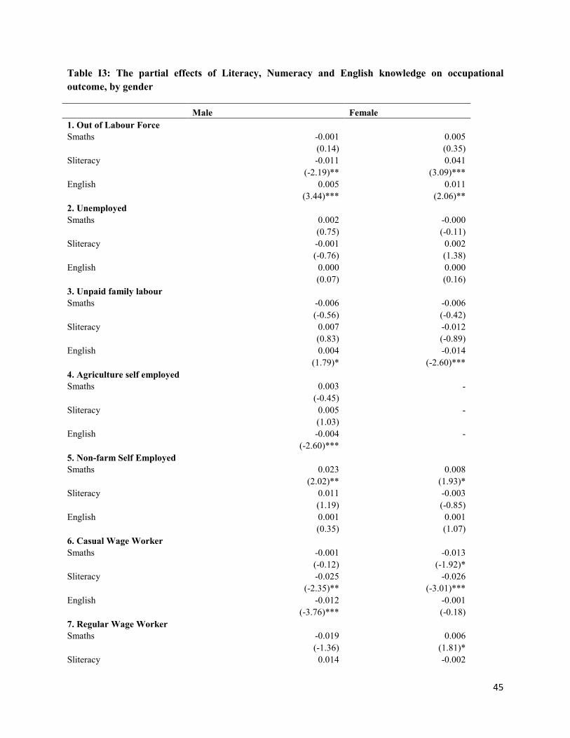
45

Table I3: The partial effects of Literacy, Numeracy and English knowledge on occupational outcome, by gender

Male Female 1. Out of Labour Force Smaths -0.001 0.005 (0.14) (0.35) Sliteracy -0.011 0.041 (-2.19)** (3.09)*** English 0.005 0.011 (3.44)*** (2.06)** 2. Unemployed Smaths 0.002 -0.000 (0.75) (-0.11) Sliteracy -0.001 0.002 (-0.76) (1.38) English 0.000 0.000 (0.07) (0.16) 3. Unpaid family labour Smaths -0.006 -0.006 (-0.56) (-0.42) Sliteracy 0.007 -0.012 (0.83) (-0.89) English 0.004 -0.014 (1.79)* (-2.60)*** 4. Agriculture self employed Smaths 0.003 - (-0.45) Sliteracy 0.005 - (1.03) English -0.004 - (-2.60)*** 5. Non-farm Self Employed Smaths 0.023 0.008 (2.02)** (1.93)* Sliteracy 0.011 -0.003 (1.19) (-0.85) English 0.001 0.001 (0.35) (1.07) 6. Casual Wage Worker Smaths -0.001 -0.013 (-0.12) (-1.92)* Sliteracy -0.025 -0.026 (-2.35)** (-3.01)*** English -0.012 -0.001 (-3.76)*** (-0.18) 7. Regular Wage Worker Smaths -0.019 0.006 (-1.36) (1.81)* Sliteracy 0.014 -0.002

46

(1.27) (-0.75) English 0.006 0.002 (1.81)* (2.46)** Note: The results are based on multinomial logits of the type reported in I4; z-statistics are in parentheses; * denotes significance at 10% level, ** significance at 5% level and *** significance at 1% level or more. Smaths denotes the test score on the short maths test (max=5) and Sliteracy denotes the test score on the short literacy test (max=5), English denotes the test score on the English test (max = 19).

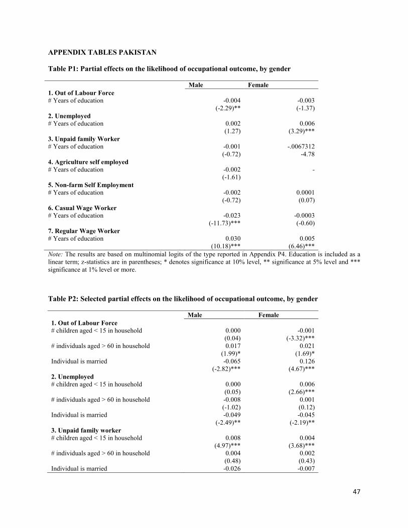
47

APPENDIX TABLES PAKISTAN

Table P1: Partial effects on the likelihood of occupational outcome, by gender

Male Female 1. Out of Labour Force # Years of education -0.004 -0.003 (-2.29)** (-1.37) 2. Unemployed # Years of education 0.002 0.006 (1.27) (3.29)*** 3. Unpaid family Worker # Years of education -0.001 -.0067312 (-0.72) -4.78 4. Agriculture self employed # Years of education -0.002 - (-1.61) 5. Non-farm Self Employment # Years of education -0.002 0.0001 (-0.72) (0.07) 6. Casual Wage Worker # Years of education -0.023 -0.0003 (-11.73)*** (-0.60) 7. Regular Wage Worker # Years of education 0.030 0.005 (10.18)*** (6.46)*** Note: The results are based on multinomial logits of the type reported in Appendix P4. Education is included as a linear term; z-statistics are in parentheses; * denotes significance at 10% level, ** significance at 5% level and *** significance at 1% level or more.

Table P2: Selected partial effects on the likelihood of occupational outcome, by gender

Male Female 1. Out of Labour Force # children aged < 15 in household 0.000 -0.001 (0.04) (-3.32)*** # individuals aged > 60 in household 0.017 0.021 (1.99)* (1.69)* Individual is married -0.065 0.126 (-2.82)*** (4.67)*** 2. Unemployed # children aged < 15 in household 0.000 0.006 (0.05) (2.66)*** # individuals aged > 60 in household -0.008 0.001 (-1.02) (0.12) Individual is married -0.049 -0.045 (-2.49)** (-2.19)** 3. Unpaid family worker # children aged < 15 in household 0.008 0.004 (4.97)*** (3.68)*** # individuals aged > 60 in household 0.004 0.002 (0.48) (0.43) Individual is married -0.026 -0.007

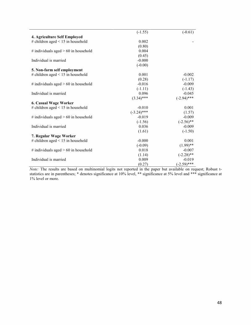
48

(-1.55) (-0.61) 4. Agriculture Self Employed # children aged < 15 in household 0.002 - (0.80) # individuals aged > 60 in household 0.004 (0.45) Individual is married -0.000 (-0.00) 5. Non-farm self employment # children aged < 15 in household 0.001 -0.002 (0.28) (-1.17) # individuals aged > 60 in household -0.016 -0.009 (-1.11) (-1.43) Individual is married 0.096 -0.045 (3.34)*** (-2.94)*** 6. Casual Wage Worker # children aged < 15 in household -0.010 0.001 (-3.24)*** (1.57) # individuals aged > 60 in household -0.019 -0.009 (-1.56) (-2.56)** Individual is married 0.036 -0.009 (1.61) (-1.50) 7. Regular Wage Worker # children aged < 15 in household -0.000 0.001 (-0.09) (1.99)** # individuals aged > 60 in household 0.018 -0.007 (1.14) (-2.28)** Individual is married 0.009 -0.019 (0.27) (-2.59)*** Note: The results are based on multinomial logits not reported in the paper but available on request; Robust t-statistics are in parentheses; * denotes significance at 10% level, ** significance at 5% level and *** significance at 1% level or more.

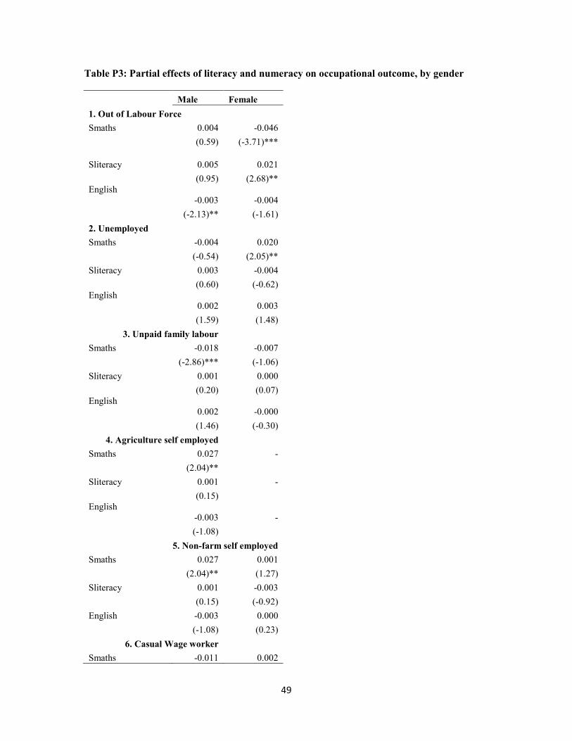
49

Table P3: Partial effects of literacy and numeracy on occupational outcome, by gender

Male Female

1. Out of Labour Force

Smaths 0.004 -0.046

(0.59) (-3.71)***

Sliteracy 0.005 0.021

(0.95) (2.68)** English -0.003 -0.004

(-2.13)** (-1.61)

2. Unemployed

Smaths -0.004 0.020

(-0.54) (2.05)**

Sliteracy 0.003 -0.004

(0.60) (-0.62) English 0.002 0.003

(1.59) (1.48)

3. Unpaid family labour

Smaths -0.018 -0.007

(-2.86)*** (-1.06)

Sliteracy 0.001 0.000

(0.20) (0.07) English 0.002 -0.000

(1.46) (-0.30)

4. Agriculture self employed

Smaths 0.027 -

(2.04)**

Sliteracy 0.001 -

(0.15) English -0.003 -

(-1.08)

5. Non-farm self employed Smaths 0.027 0.001

(2.04)** (1.27)

Sliteracy 0.001 -0.003

(0.15) (-0.92)

English -0.003 0.000

(-1.08) (0.23)

6. Casual Wage worker

Smaths -0.011 0.002

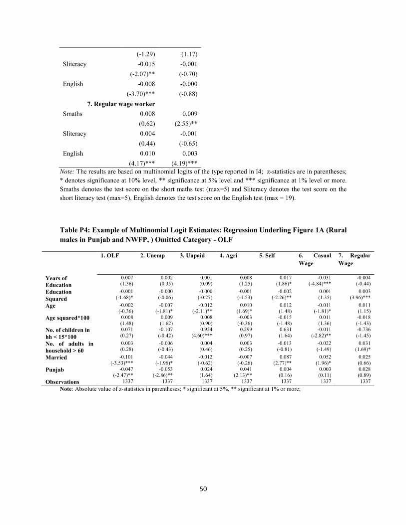
50

(-1.29) (1.17)

Sliteracy -0.015 -0.001

(-2.07)** (-0.70)

English -0.008 -0.000

(-3.70)*** (-0.88)

7. Regular wage worker

Smaths 0.008 0.009

(0.62) (2.55)**

Sliteracy 0.004 -0.001

(0.44) (-0.65)

English 0.010 0.003

(4.17)*** (4.19)*** Note: The results are based on multinomial logits of the type reported in I4; z-statistics are in parentheses; * denotes significance at 10% level, ** significance at 5% level and *** significance at 1% level or more. Smaths denotes the test score on the short maths test (max=5) and Sliteracy denotes the test score on the short literacy test (max=5), English denotes the test score on the English test (max = 19).

Table P4: Example of Multinomial Logit Estimates: Regression Underling Figure 1A (Rural males in Punjab and NWFP, ) Omitted Category - OLF

1. OLF 2. Unemp 3. Unpaid 4. Agri 5. Self 6. Casual Wage

7. Regular Wage

Years of Education

0.007 (1.36)

0.002 (0.35)

0.001 (0.09)

0.008 (1.25)

0.017 (1.86)*

-0.031 (-4.84)***

-0.004 (-0.44)

Education Squared

-0.001 (-1.68)*

-0.000 (-0.06)

-0.000 (-0.27)

-0.001 (-1.53)

-0.002 (-2.26)**

0.001 (1.35)

0.003 (3.96)***

Age -0.002 (-0.36)

-0.007 (-1.81)*

-0.012 (-2.11)**

0.010 (1.69)*

0.012 (1.48)

-0.011 (-1.81)*

0.011 (1.15)

Age squared*100 0.008 (1.48)

0.009 (1.62)

0.008 (0.90)

-0.003 (-0.36)

-0.015 (-1.48)

0.011 (1.36)

-0.018 (-1.43)

No. of children in hh < 15*100

0.071 (0.27)

-0.107 (-0.42)

0.954 (4.60)***

0.299 (0.97)

0.631 (1.64)

-0.011 (-2.82)**

-0.736 (-1.45)

No. of adults in household > 60

0.003 (0.28)

-0.006 (-0.43)

0.004 (0.46)

0.003 (0.25)

-0.013 (-0.81)

-0.022 (-1.49)

0.031 (1.69)*

Married -0.101 (-3.53)***

-0.044 (-1.96)*

-0.012 (-0.62)

-0.007 (-0.26)

0.087 (2.77)**

0.052 (1.96)*

0.025 (0.66)

Punjab -0.047 (-2.47)**

-0.053 (-2.86)**

0.024 (1.64)

0.041 (2.13)**

0.004 (0.16)

0.003 (0.11)

0.028 (0.89)

Observations 1337 1337 1337 1337 1337 1337 1337 Note: Absolute value of z-statistics in parentheses; * significant at 5%, ** significant at 1% or more;