Recommendation WG 2.99.052 (Supersedes Rec. WG …nsma.org/wp-content/uploads/2016/05/WG2-99-052.pdf · October 2000 Source: Working Group 2 Recommendation WG 2.99.052 (Supersedes

October 2000 Source: Working Group 2

Recommendation WG 2.99.052(Supersedes Rec. WG 2.89.023)

OHLOSS PATH LOSS COMPUTATIONwith

OHLOSS TUTORIAL(formerly Rep. WG 2.95.010)

www.nsma.org

http://www.nsma.org/

RECOMMENDATION

Subject Area: OHLOSS

Title: OHLOSS Path Loss Computation

Recommendation:

The NSMA Working Group 2 OHLOSS TUTORIAL of 1999 should be utilized in the construction of newversions of Over-the-Horizon Loss (OHLOSS) programs or to bring existing programs into compliance.Use of the OHLOSS TUTORIAL should result in OHLOSS calculations that yield answers with a highdegree of agreement with other members of the Association. This recommendation supersedes theNSMA recommendation entitled “OHLOSS Path Loss Computation Flowchart”* that was approved onApril 25, 1989.

Recommended: WG2.99.052

Approved: August 6, 1999

Note: The OHLOSS TUTORIAL (REP.WG2.95.010) is now part of this Recommendation WG2.99.052

* Recommendation WG2.89.023

National Spectrum Managers Association OHLOSS TUTORIAL

INTRODUCTION................................................................................................................................................................. 1

PROPAGATION MECHANISMS INCORPORATED IN THE OHLOSS COMPUTATION ....................................... 2

Diffraction Loss...................................................................................................................................................... 2

Terrain Models ....................................................................................................................................................... 3

Single Knife Edge ............................................................................................................................................ 3

Isolated Obstacle (Single Knife Edge with Radius) ........................................................................................ 3

Effective Knife Edge........................................................................................................................................ 4

Double Knife Edge........................................................................................................................................... 4

Multiple Knife Edge......................................................................................................................................... 4

Irregular Terrain ............................................................................................................................................... 5

NSMA OHLOSS Terrain Models ......................................................................................................................... 5

Tropospheric Scatter Loss...................................................................................................................................... 6

OHLOSS CALCULATION PROCEDURE........................................................................................................................ 6

INPUT PARAMETERS ....................................................................................................................................................... 6

TERRAIN DATA EXPANSION......................................................................................................................................... 7

PATH PARAMETERS......................................................................................................................................................... 7

Transhorizon Path Geometry ................................................................................................................................. 7

Effective Earth Radius............................................................................................................................................ 8

Earth Curvature....................................................................................................................................................... 9

Horizon Elevation Angles ...................................................................................................................................... 9

Cross Over Angle of Horizon Rays ..................................................................................................................... 10

Effective Antenna Heights ................................................................................................................................... 10

FREE SPACE PATH LOSS............................................................................................................................................... 11

REFERENCE DIFFRACTION LOSS............................................................................................................................... 12

Single Knife Edge Diffraction Loss (SKE) ......................................................................................................... 12

Isolated Obstacle Diffraction Loss (ISOL).......................................................................................................... 13

Obstacle Radius .............................................................................................................................................. 13

Double Knife Edge Diffraction Loss (DKE)....................................................................................................... 14

Height Gain Terms ............................................................................................................................................... 15

Rough Earth Diffraction....................................................................................................................................... 15

REFERENCE TROPOSPHERIC SCATTER LOSS......................................................................................................... 17

nsma October 2000 i WG 2.95.010

REFERENCE COMBINED LOSS .................................................................................................................................... 17


MEDIAN TOTAL TRANSMISSION LOSS .................................................................................................................... 18

ATMOSPHERIC ABSORPTION LOSS........................................................................................................................... 19

LONG TERM TIME VARIABILITY FACTORS............................................................................................................ 20

Diffraction Type - Single Knife Edge, Single Rounded Obstacle, and Double Knife Edge............................................. 20

Troposcattering Type - Irregular Terrain or Troposcatter .................................................................................................. 21

95 Percent Confidence Factor Adjustment .......................................................................................................... 22

Variability Limitation Referenced to Free Space ................................................................................................ 22

TERRAIN DATA BASES.................................................................................................................................................. 22

OHLOSS SAMPLE CALCULATIONS............................................................................................................................ 23

OHLOSS REPORT FORMAT........................................................................................................................................... 23

nsma October 2000 ii WG 2.95.010


INTRODUCTION

The primary purpose of “Over the Horizon Loss” (OHLOSS) computations is to more accurately predict the loss between an interfering transmitter antenna and a victim receiver antenna. This tutorial discusses various factors that affect point-to-point propagation and describes the related calculation procedures and algorithms.

The terrain and other obstacles have a bearing on the propagation of radio energy from one point to another, particularly at microwave frequencies, where the ground wave is not important. When a radio path is obstructed by mountains, trees, buildings, etc., the field intensity obtained at the receiving point is affected by a variety of factors that cause electromagnetic waves to be redirected. The effects on propagation depend upon many things, including the position, shape and height of obstacles, and the nature of the underlying terrain. The standard approach in estimating radio transmission loss is to calculate the expected line-of-sight transmission attenuation between two points, and then include additional effects caused by over-the-horizon propagation.

Three mechanisms propagate microwave energy beyond the radio horizon (the first point of grazing or blockage on the line between the transmitter and receiver): reflections, atmospheric (tropospheric) scattering, and diffraction over obstacles. The additional loss above free-space loss caused by these propagation mechanisms can be used to predict the signal level arriving at a receiver from an interfering transmitter.

It is useful to discuss the effect of some commonly experienced obstacles to illustrate the nature of obstruction losses. Trees for example, cause dispersion of energy and affect the vertical clearance. At grazing, they look similar to a knife edge in diffraction theory, and such a single obstacle along the path will result in about a 6 dB additional loss. When trees are obstructions, they are normally considered to be totally blocking. The effect of man-made obstacles depends entirely upon their shape and position. Few objects are microwave-transparent, but those that are can be ignored.1

NSMA Working Group 2 establishes guidelines under which an expected obstruction loss, known as OHLOSS, may be calculated and added to the free space loss to clear interference cases. Any radio path that has less clearance than 60% of its first Fresnel zone anywhere along its entire length, caused by any obstruction including buildings, trees, terrain and the curvature of the Earth, is a candidate for OHLOSS analysis. Graphs and computer programs have been developed to aid in the calculation of OHLOSS. The OHLOSS computation takes available terrain and obstruction data into account and will report if the path is line-of-sight or blocked, the height of the possible obstructions, and if a single or double knife edge exists on the path. In many cases, the OHLOSS is adequate to improve the calculated line-of-sight Carrier-to-Interference (C/I) ratio enough to meet objectives.2 It is important that the methodology behind an OHLOSS analysis is a uniform one that is recognized by all frequency coordinators.

1 Propagation on point-to-point microwave paths (both desired and interfering) longer than a few miles is typically studied for various degrees of atmospheric refraction, which is represented in the computations as different apparent earth curvatures (using the variable K, which represents the ratio of apparent to actual Earth radius). A grazing path is one where one or more obstructions just touch the line between the end point antennas, taking into account the apparent Earth curvature (value of K) used in a particular study. In a blocked path, one or more obstructions intersects and crosses this line.

2 Since large numbers of microwave receivers are potentially affected by a proposed new transmitter installation (for example, at 6 GHz the coordination distance, within which paths to all potential victim receivers must be studied, ranges from 125 to 250 miles), common practice is to initially study interference assuming a line-of-sight (LOS) path loss. This simplified analysis typically will clear most potential interference cases. For those cases remaining, the more complex OHLOSS analysis is invoked; additional loss predictions from that analysis are then added to the LOS loss figure to determine if the case can be cleared.

nsma October 2000 Page 1 of 25 WG 2.95.010


A uniform standard for OHLOSS calculations will reduce contention among coordinators and allow a greater sense of stability within the frequency coordination process. If frequency coordinators use an OHLOSS tool that is too conservative, frequency utilization will be poor. If frequency coordinators use an OHLOSS tool that over estimates loss, cases of interference will become prevalent.

Uniformity in the results from OHLOSS computations made by different coordinators, using the same input data, is a key goal of NSMA Working Group 2. While the OHLOSS computation processes are developed by WG-2, the computer programs employed by each user to calculate results may be unique. Therefore the working group efforts are directed at (1) achieving consensus on the computational process and (2) providing a structure where the results of various mechanized coordination systems can be compared for uniformity. Since a wide variety of telecommunication companies are represented in the consensus building process, NSMA has the ability to produce a recommendation that will be widely accepted and will serve the spectrum management industry well. This process benefits all users by fostering efficient use of the spectrum and minimizing the probability of harmful interference.

PROPAGATION MECHANISMS INCORPORATED IN THE OHLOSS COMPUTATION

Transmission beyond the horizon is controlled by three propagation mechanisms: diffraction, tropospheric scatter and reflection. Of the three, reflection is the least common and least predictable and is not currently included in OHLOSS analysis. Diffraction and tropospheric scatter are included and are treated as independent phenomena. Tropospheric scatter is usually the controlling factor on paths longer than 70 miles, whereas on shorter paths, the overall loss is most often controlled by diffraction.

Diffraction and tropospheric scatter loss are first calculated under average atmospheric conditions. This calculation requires the value of the atmospheric refractivity at sea level for the path. This can be determined through the use of a surface refractivity map. Once the two path end points are found on the map and the corresponding contours are chosen, the higher of the two values is used for the path refractivity.

After both the diffraction and scatter losses are computed, they are combined by considering the losses as two resistors in parallel. If the tropospheric scatter loss is much greater than the diffraction loss, then the combined loss will nearly equal the diffraction loss. Conversely, if the diffraction loss is much greater than the tropospheric scatter loss, then the result will be approximately the tropospheric scatter loss. In the case of equal diffraction and tropospheric scatter loss, the combined loss is 3 dB less than either value. This combined loss will vary as atmospheric conditions change, therefore once the median combined loss is found, the next step is to determine the expected loss for various percentages of time. This is accomplished using empirical statistics based on measured data, as described in the section of this tutorial on long term variability.

Diffraction Loss

The concept of diffraction is illustrated in Figure 1. A wave front from a transmitter strikes an obstruction on the path and creates a secondary radiation source at the peak of the obstruction. This new wave is called a Huygens's source or a diffraction wave. The diffraction wave propagates into the geometric shadow region behind the obstruction and also into the unobstructed region. In the shadow region, the diffracted wave amplitude decreases as the angle of the wave extends deeper into the shadow region. In the unobstructed region, the diffraction wave and the initial wave source combine to produce positive and negative receive signal reinforcement.



Directedcone of energy

from atransmittingantenna

Wave crests Wave troughs

Positive and negativereinforcement

Diffractionwave front

(unobstructedregion)

Diffractionwave front(apparent

shadow region)

Field strength ifno obstructionpresent

Fieldenergy

1.0

Apparentshadow region El

evation

Figure 1 Diffraction Loss

Terrain Models

Unfortunately, a general solution for diffraction loss over irregular terrain is not available. Exact solutions have been developed for the two limiting cases of a path obstructed by an ideal knife edge and a path obstructed by a smooth spherical Earth. The smooth Earth diffraction is calculated by a residue series which converges rapidly for paths well beyond the horizon and very slowly for paths that are nearly line of sight. Due to the complex nature of this series, many algorithms use only the first term of the series.

Most real terrain profiles fall somewhere in between these two limiting cases. A diffraction loss calculation starts by characterizing the terrain so as to apply the two basic algorithms to different portions of the profile.

Single Knife Edge

Figure 2 Single Knife Edge

Figure 3 Knife Edge with Radius

A path can be characterized as a knife edge if the transmit and receive horizons share a common point. In this case, the diffraction loss is calculated as an ideal knife edge.

Isolated Obstacle (Single Knife Edge with Radius)

A path consisting of single obstruction, with a relatively small distance between the transmit and receive horizons, can be treated as an ideal knife edge with an additional factor to account for the finite size of the obstruction. In this model, an estimate of the obstacle radius is required. This model is valid if the obstacle is isolated from the transmit and receive sites. An obstruction formed by the bulge of a smooth Earth profile is not isolated.



Figure 4 Effective Knife Edge

Figure 4 Effective Knife Edge

Effective Knife Edge

In this model, the transmit and receive horizon rays are extended to their intersection. Diffraction loss is calculated as an ideal knife edge at the intersection of the horizons.

Double Knife Edge

Figure 5 Double Knife Edge (Epstein - Peterson)

Figure 6 Double Knife Edge (Deygout)

Figure 7 Multiple Knife Edge

The diffraction loss is calculated as the sum of two ideal knife edges in this model. There are two models for calculating a double knife edge.

Epstein-Peterson model

In this model, the individual knife edges calculations are referenced to the horizons of the knife edge under consideration.

Deygout Model

In the Deygout model, the knife edge diffraction of the major obstacle is first calculated as if the second obstacle did not exist. The contribution of the secondary obstacle is calculated referenced to its horizons. The two knife edge losses are added to produce the total loss.

Multiple Knife Edge

In this model the terrain is treated as a succession of knife edges using the Epstein - Peterson method. An upper limit is usually imposed on the number of knife edges.



Irregular Terrain

Figure 8 Irregular Terrain

If the terrain cannot be characterized by any of the knife edge models, a default irregular terrain is used. Two common irregular terrain models are described below.

Rough Earth Diffraction

The path is divided into the following four regions:

• Transmit site to its horizon

• Transmit horizon to the crossover point of the horizon rays.

• Crossover point of the horizon rays to the receive horizon

• Receive horizon to the receive site.

Effective Earth radii are then determined for each of these regions. The smooth Earth diffraction loss is calculated for each region and the results are combined to produce the overall diffraction loss.

Longley and Rice

In the Longley and Rice model, the path is characterized by the effective antenna heights, horizon elevation angles and the terrain roughness. Two distances are empirically determined beyond the line of sight.

At each distance, smooth Earth and double knife edge diffraction loss are calculated and combined using an empirical weighting factor. The weighting factor is a function of the terrain roughness. On relatively smooth paths, the smooth Earth diffraction loss will control and the double knife edge value will control on paths with large elevation changes.

A linear relationship between distance and diffraction loss is determined using the loss values at the two distances. The diffraction loss is calculated by interpolating this line at the actual path length.

NSMA OHLOSS Terrain Models

The following terrain models are used in the current NSMA recommendation for OHLOSS calculations:

• Single knife edge

• Single knife edge with radius

• Double knife edge using the Epstein-Peterson model

• Rough Earth diffraction



Tropospheric Scatter Loss

As the wave passes through the troposphere, both refraction and reflection will occur. The bending of the radio wave is determined by the atmosphere refractivity gradient. The reflections are due to the interaction of the wave with the molecules of air within the troposphere. If the wave encounters an atmospheric layer with different refractivity than its surroundings, specular reflection may occur; however, for the most part, the reflections are diffuse. The aggregate sum of these reflections constitute the tropospheric scatter energy.

Tropospheric scatter is a phenomena that depends on the region of the atmosphere that the transmitter can illuminate and the receiver can see. Therefore, tropospheric scatter loss depends only on the locations of the transmit and receive horizons and the overall path length. No other terrain parameters are involved. The directivity of the transmit and receive antennas are taken into account by their gains. The calculations assume that the antenna boresights are essentially horizontal.

FrequencyPolarizationAntenna HeightsAntenna GainsK or Surface Refractivity NsGround characteristicsClimatic region

Horizon anglesCross Over AngleEffective Antenna Heights

InputParameters

TerrainProfile

ExpandTerrainData

Calculate Path Parameters

ReferenceDiffractionLoss

ReferenceTroposphericScatter Loss

Reference Combined Loss

Median Combined Loss

Free Space Loss

Atmospheric Adsorption Loss

Total Median Loss

Time Variability

Figure 9 OHLOSS Calculation Procedure

OHLOSS CALCULATION PROCEDURE

Figure 9 shows the basic components and the sequence of calculations in an OHLOSS analysis. Each step is described in the following sections.

The reference diffraction and tropospheric scatter loss are calculated and combined. This combined loss is adjusted for regional geographic effects to produce a median value of the combined loss.

The total median loss is calculated as the sum of the combined median loss, free space loss and the atmospheric absorption loss.

The time variability is calculated as a cumulative probability distribution of loss as a function of time using 50% and 95% confidence factors.

INPUT PARAMETERS

The following input parameters are required in an OHLOSS calculation:

Frequency Polarization

Antenna Heights Antenna Gains

Surface refractivity (Ns) or effective Earth radius factor (K)

Ground characteristics (conductivity and dielectric constant)

Climate Region



TERRAIN DATA EXPANSION

0.1 mile minimum

User pointsExpanded points

Figure 10 Terrain Profile Expansion

In order to accurately calculate the location of the transmit and receive horizons, a maximum spacing between terrain data points of 0.1 mile is required.

The actual distance between the transmit and receive horizons determines if the obstacle radius is to be included in single knife edge cases.

Figure 10 shows a section of a terrain profile with intermediate points spaced at 0.1 mile increments. These intermediate points are determined by linear interpolation of the adjacent input profile data points.

PATH PARAMETERS

Figure 11 Transhorizon Path Geometry

Transhorizon Path Geometry

Figure 11 shows the basic geometry of a transhorizon path. By convention, the transmit site is on the left and the receive site on the right side of the diagram. The terminology is defined below and is used throughout this section.

hts TX antenna height AMSL (Above Mean Sea Level)

hrs RX antenna height AMSL



dLt TX horizon distance

dSt TX horizon to cross-over point distance

hLt TX horizon elevation level

Θet TX horizon elevation angle

dLr RX horizon distance

dSr RX horizon to cross-over point distance

hLr RX horizon elevation

Θer RX horizon elevation angle

d great circle arc path length

Θ cross over angle of the horizon rays

dS horizon to horizon distance

d1 distance from the TX site to the cross over point of the horizon rays

d2 distance from the RX site to the cross over point of the horizon rays

a0 Earth radius (6370 km)

a effective Earth radius

All distances and elevations are expressed in the same units, usually kilometers. All angles are expressed in radians and it is assumed that all angles are small so that tan( )Θ Θ≈ . In addition, the following relationships hold between the various distances:

d d d d d d d d d d d d dLt St Lr Sr S St Sr Lt S Lr1 2= + = + = + = + +

Effective Earth Radius

Due to the normally decreasing index of refraction of the atmosphere with increasing elevation, microwave radiation traveling over the surface of the Earth tends to propagate in a slightly downward heading arc instead of a straight line. This slight bending of the microwave rays can be accounted for by assuming the radius of the Earth is larger than its actual value and that the rays travel in a straight line. This assumed larger radius of the Earth is called the effective Earth radius.



The effective Earth radius, a, is calculated as the actual Earth radius, (ao = 6370 km) times the Earth radius factor K. This K factor is typically about 4/3. (The K factor should not be confused with the K parameter used later in this tutorial.)

a K ao= ⋅ (1)

Alternately, a, can be expressed in terms of the surface refractivity, Ns, as:

a a1 0.04665 e

o0.005577 N s

=− ⋅ ⋅

(2)

Refractivity is a measure of how much the index of refraction exceeds one. It is defined as where n is the index of refraction. The surface refractivity N

N n= − ×( )1 106

s is defined as the refractivity of the atmosphere at ground level. A nominal value for Ns in a continental temperate climate is 301, however surface refractivity can vary from about 250 to 400 in different regions of the world. Section 4 in Tech Note 101[1] discusses the K factor and surface refractivity in more detail than this tutorial.

Earth Curvature

When examining a path profile to determine the horizon points the effective curvature of the Earth must be taken into account. This can be done by adding a parabolic approximation of the effective Earth curvature to the path profile terrain data before finding horizons. One such parabolic function that can be used is:

hd d

ad d d

ad d d

aEt r t t r r= =

−=

−2 2 2

( ) ( ) (3)

where

hE effective Earth curvature in kilometers

dt distance from the transmit site in kilometers

dr distance from the receive site in kilometers

a effective Earth radius in kilometers

The effective Earth curvature, hE, should be added to all terrain elevation points along the path profile before determining horizon points or Fresnel zone clearances. It is important the path profile points are not spaced too far apart in order to properly account for the effects of the effective Earth curvature, and is the reason for adding the interpolated terrain points described in the TERRAIN DATA EXPANSION section of this tutorial.

Horizon Elevation Angles

These angles are defined to be positive if the horizon ray leaves the antenna in an upward direction and negative if the horizon ray leaves in a downward direction. The elevation angles shown in Figure 11 have negative values. The transmit and receive elevation angles can be calculated by:



etLt ts

Lt

Lt

erLr rs

Lr

Lr

h hd

da

h hd

da

≈Θ

Θ

−−

≈−

−

2

2

[

[

radians]

radians]

(4)

where all heights and distances are expressed in the same units of measure. h h h hLt Lr ts rs, , , d d aLt Lr, ,

The angles, α and , are calculated as: o βo

o etts rs

o errs tsh h

dd2a

h hd

d2a

β≈ +−

+ ≈ +α−

+Θ Θ (5)

Cross Over Angle of Horizon Rays

The cross over angle of the horizon rays, Θ, is sometimes referred to as the scatter angle and is always positive for a transhorizon path.

Θ Θ Θ= + = + +

≈−

+−

++

+

o o et er

Lt ts

Lt

Lr rs

Lr

Lt Lr S

da

h hd

h hd

d da

da

α β

2

(6)

The distances, and , from the cross over point of the horizon rays to the transmit and receive sites are given by: d1 d2

1 2d d do o≈ ≈dβ αΘ Θ

(7)

Effective Antenna Heights

80% dlr

dlrdlt80% dlt

hrs hre

hts

hte

Average

Figure 12 Effective Antenna Heights

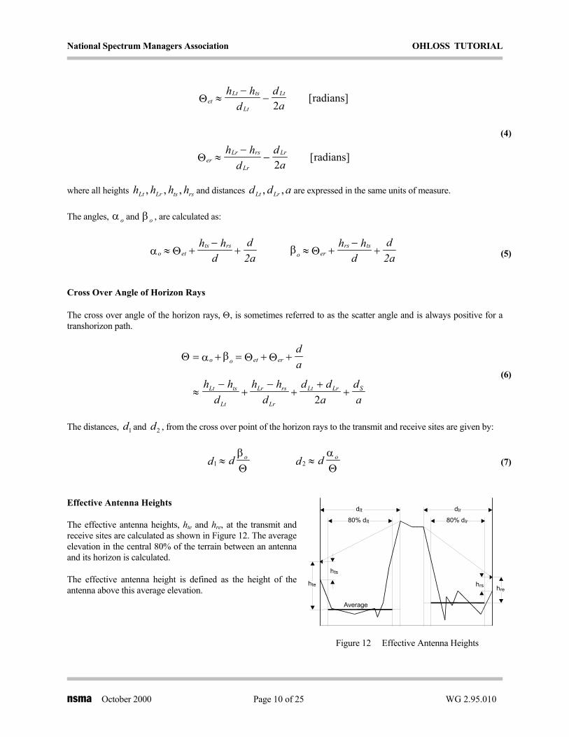
The effective antenna heights, hte and hre, at the transmit and receive sites are calculated as shown in Figure 12. The average elevation in the central 80% of the terrain between an antenna and its horizon is calculated.

The effective antenna height is defined as the height of the antenna above this average elevation.



FREE SPACE PATH LOSS

The free space path loss in dB between two isotropic radiators is given by:

L ff MHz= d+ +32 45 20 20. log( ) log( ) (8)

where fMHz frequency in MHz d path length in kilometers

or alternatively:

(9) L ff = d+ +96 6 20 20. log( ) log( )

where f frequency in GHz d path length in miles



REFERENCE DIFFRACTION LOSS

Figure 13 shows a logic diagram used to analyze the terrain profile and to determine the required algorithm(s) to calculate the reference diffraction loss. The criteria used for each branch of the logic diagram are described below.

N Y

N Y

CalculateHG 1/2

CalculateA = ISOLd

CalculateHG 1/2

CalculateA = SKEd

ISOL?

DKE?

SKE?

CalculateA = DKEd

CalculateHG 1/2

A = RED A = A + HG 1/2d

N Y

Figure 13 Reference Diffraction Loss

In Figure 13 the terms are defined as follows:

SKE single knife edge

ISOL isolated obstacle

DKE double knife edge

HG 1/2 height gain terms used with SKE, ISOL and DKE to account for lack of clearance between a site and its horizon.

RED rough Earth diffraction

Single Knife Edge Diffraction Loss (SKE)

The path is classed as a single knife edge if the transmit and receive horizons are at the same point on the profile. Diffraction loss is calculated using the Fresnel-Kirchhoff knife edge formula given in equation (10).

A A

+ +

+

+

d

2

2= ≈

− ≤ <

− ≤ <

≤

( , )

. . . ; .

. . . ; .

. log( ) ; .

ν

ν ν ν

ν ν ν

ν ν

0

6 02 9 00 165 0 8 0

6 02 911 127 0 2 4

12 953 20 2 4

(10)

The term is given by: ν

v = d

f d dd

0 0

MHz

2

2 583 1 2

tan( ) tan( )

.

α β λ

≈ ⋅⋅

Θ

(11)

where the distances and the wavelength d d d, ,1 2 λ are in kilometers.



Isolated Obstacle Diffraction Loss (ISOL)

If the distance between the transmit and receive horizons is greater than zero and less than or equal to 0.3 miles, the effects of the obstacle radius are considered. In this case, additional terms are added to the basic knife edge diffraction formula in equation (10) to account for the finite radius of the obstruction.

The isolated obstacle diffraction loss is given by:

A A , = A , + A , + Ud = ( ) ( ) ( ) ( )ν ρ ν ρ νρ0 0 (12)

where

A , 2 3( ) . . . .0 6 02 5556 3418 0 256ρ ρ ρ ρ≈ + + + (13)

U x

x x x x

x x x x

x x

( )

. . . . ;

. . . . ;

. ;

≈

+ − − ≤

+ − − < ≤

− <

1145 219 0 206 6 02 3

1347 1058 0 048 6 02 3 5

20 18 2 5

2 3

2 3 (14)

ρ ≡ ⋅ ⋅ ⋅⋅

0 676 1 3 1 6. / /R f dd dMHz

-

1 2 (15)

and R is the radius of the obstacle in kilometers.

Obstacle Radius

If the horizons are symmetric about the rounded obstacle so that d dSt Sr= then the radius of the rounded obstacle can be computed as in equation 7.10 from Tech Note 101[1]:

RdS≈Θ

(16)

If the horizons are not symmetric so that dSt Srd≠ then equation 7.11 from Tech Note 101[1] suggests that the radius of the rounded obstacle can be computed as:

Rd d d

d dS St Sr

St Sr≈ ⋅

+Θ2

2 2 (17)

Notice that equation (17) reduces to equation (16) if d dSt Sr= . Unfortunately equation (17) can yield very small values for the radius if the horizons are quite asymmetric. It has been found that a weighted average of the symmetric and asymmetric equations for the radius will produce better results than either equation by itself. Based on sample paths



that have been tested, a good compromise is to use 1/3 of the symmetric equation and 2/3 of the asymmetric equation to compute the radius of the obstacle. This results in:

( )Rd d d d

d dS S St Sr

St Sr

≈ ⋅+

+Θ

2

2 2

23

(18)

Double Knife Edge Diffraction Loss (DKE)

B1 Segmentst

2 Segmentnd

Figure 14 Double Knife Edge

A DCA path is classified as a double knife edge if line of sight exists between the transmit and receive horizons. There are no clearance criteria for the terrain between the two horizons.

The diffraction loss is calculated as a double knife edge using the Epstein- Peterson method. The obstacle radius is not calculated on a double knife edge path.

The diffraction loss is taken as the sum of the two individual knife edges.

The method is shown in Figure 14. The diffraction loss of each knife edge is calculated over the profile segment formed by the horizons of the knife edge. In Figure 14, the knife edge located at B, is calculated over the profile segment from A to C. The knife edge located at C, is calculated over the segment from B to D.

The double knife edge diffraction loss can be computed as:

A A Ad = +( , ) ( , )ν ν1 20 0 (19)

where

1 1 2 2+ +d d d dMHzLt S

MHzLr S

ν ν2 583 2 583≈ ⋅ ≈ ⋅. .Θ Θfd d

fd dLt S Lr S

(20)

Θ Θ Θ Θ1 22 2

2 2

≈ +−

− ++

≈ +−

− ++

≈−

+−

++

≈−

+−

++

etLt Lr

S

S Lt Ser

Lr Lt

S

S Lr S

Lt ts

Lt

Lt Lr

S

Lt S Lr rs

Lr

Lr Lt

S

Lr S

h hd

da

d da

h hd

da

d da

h hd

h hd

d da

h hd

h hd

d da

(21)

and all heights and distances are in kilometers. h h h hLt Lr ts rs, , , d d d aLt S Lr, , ,



Height Gain Terms

If the propagation path has been classified as a single knife edge, double knife edge or an isolated obstacle, then a clearance test is required between the transmit and receive sites and their respective horizons to complete the reference diffraction loss calculation. A first Fresnel zone (100% F1) reference is constructed between the antenna and its horizon for both the transmitter and receiver. If more than 50% of the terrain in this region is above the first Fresnel zone reference, then the additional loss due to this lack of clearance is calculated and added to the diffraction loss. This additional loss is referred to as the height gain terms; however the result is always a loss and does not consider signal enhancement due to foreground reflections.

The first Fresnel zone is defined as the volume of a prolate spheroid whose major axis lies on the horizon ray and whose focii are located at the antenna and horizon point. The distance from the antenna to the surface of the first Fresnel zone and then to the horizon point is one half wavelength greater than the distance between the antenna and horizon point. The radius of the Fresnel zone, that is the required clearance around the horizon ray is a function of the distance from the antenna. The first Fresnel zone radius can be computed in kilometers as:

Fd d d

dF

d d dd

d d df d

d d df d

t Lt t

Lt

r Lr r

Lr

t Lt t

MHz Lt

r Lr r

MHz Lr

1 1

0 5475 0 5475

≈−

≈−

≈−⋅

≈−⋅

λ λ( ) ( )

.( )

.( )

or (22)

A A G h G h d= − −( ) ( )1 2

1 3 1 3/ /

where dt is the distance from the transmitter and dr is the distance from the receiver. All distances dt, dLt, dr, dLr and the wavelength λ are in kilometers.

The reference diffraction loss is calculated using two height gain terms, one for the transmitting antenna and a second for the receiving antenna as:

(23)

where

( ) ( )h f a h h f a hMHz te MHz re12

1 22

25 74 5 74= =. . (24)

a dh a d

hLt

te

Lr

re1

2

2

2

2 2= = (25)

If more than 50% of the terrain between the antenna and its horizon has first Fresnel zone clearance, that height gain term , , is taken to be zero. Otherwise the numerical data and approximate parametric formulas presented in Annex 1 of this tutorial can be used to compute the height gain terms. Details of this calculation are presented in Tech Note 101[1] sections 7.2 and 7.4

G h( )

Rough Earth Diffraction

If the path cannot be classified as a single knife edge, double knife edge or an isolated obstacle, the irregular terrain algorithm is used as a default to calculate the diffraction loss.



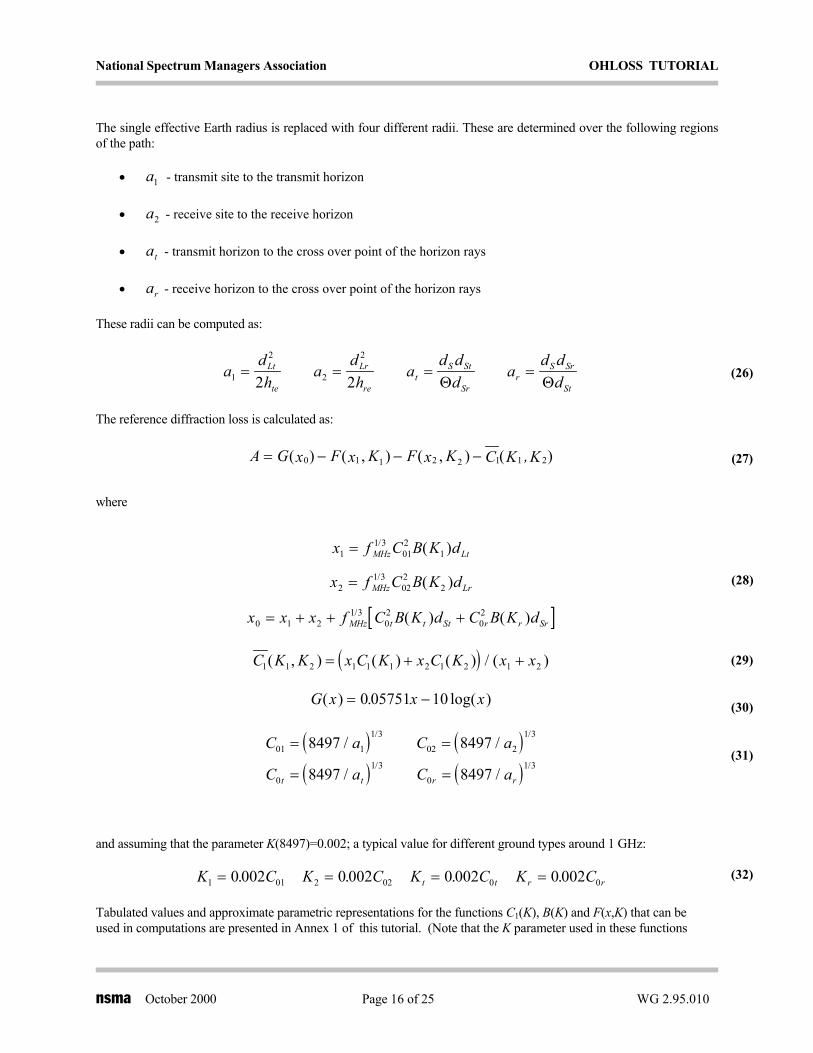
The single effective Earth radius is replaced with four different radii. These are determined over the following regions of the path:

• - transmit site to the transmit horizon a1

at

ar

• - receive site to the receive horizon a2

• - transmit horizon to the cross over point of the horizon rays

• - receive horizon to the cross over point of the horizon rays

These radii can be computed as:

adh

adh

ad d

da

d dd

Lt

te

Lr

ret

S St

Srr

S Sr

St1

2

2

2

2 2= = = =

Θ Θ

[ ]x f C B K d

x x x f C B K d C B K d

MHz Lr

MHz t t St r r Sr

2 02 2

0 1 21 3

02

02= + + +/

( )

( ) ( )

(26)

The reference diffraction loss is calculated as:

A G x F x K F x K C K ,K= − − −( ) ( , ) ( , ) ( )0 1 1 2 2 1 1 2

G x x x( ) . log( )= −0 05751 10

(27)

where

x f C B K dMHz Lt11 3

012

1

1 3 2

=

=

/

/

( )

(28)

( ) ( )C a C at t r r0 08497 8497= =/ /

K C K C K C K002 0 002 0 002 0= = = =. . .

( )C K K x C K x C K x x1 1 2 1 1 1 2 1 2 1 2( , ) ( ) ( ) / ( )= + + (29)

(30)

( ) ( )C a C a01 11 3

02 21 3

1 3 1 3

8497 8497= =/ // /

/ /

Ct t r r1 01 2 02 0 00 002

(31)

and assuming that the parameter K(8497)=0.002; a typical value for different ground types around 1 GHz:

(32) .

Tabulated values and approximate parametric representations for the functions C1(K), B(K) and F(x,K) that can be used in computations are presented in Annex 1 of this tutorial. (Note that the K parameter used in these functions



should not be confused with the effective Earth radius K factor.) Section 8.2 in Technical Note 101[1] discusses these calculations along with figures 8.1 through 8.12.

REFERENCE TROPOSPHERIC SCATTER LOSS

The reference tropospheric scatter loss, Ls, is given by:

( ) ( )[ ]sdL L N e+ = − −36 301 40/θ

x x x

0 ( ) . . . log( );

. . log( );

+ + ≤ <

+ + ≤

129 5 0 212 37 5 10 70

119 2 0157 45 70

f MHz sf d F d+ − + −20 20 010log log( ) ( ) .Θ (33)

where

F x

x x x

x x x

. . log( ); .

= + + ≤ <

13582 0 33 30 0 01 10

(34)

and

Ns surface refractivity

d path length in kilometers

Θ cross over angle of the horizon rays (scatter angle) in radians

Note that equation (33) represents the total transmission loss between the transmit and receive sites due to tropospheric scatter and includes the free space loss.

REFERENCE COMBINED LOSS

Diffraction and tropospheric scatter are treated as two independent transmission mechanisms. Tropospheric scatter loss represents the limiting value of the transmission loss. The combined loss, Lc, is calculated as:

[ ]cA LL = S− +− −10 10 1010 10log / / (35)

where

A reference diffraction loss

Ls reference tropospheric scatter loss



MEDIAN TOTAL TRANSMISSION LOSS

The median transmission loss, Ln(0.5), is obtained by applying a climatic adjustment factor to the reference combined loss. The climatic adjustment factor is defined as:

( )n c n eL L - V ,d( . ) .0 5 0 5= (36)

where

n denotes a particular climatic region.

de effective distance

The effective distance in Km is given by:

d

dd d

d d d

d d d d d de L S

L S

L S L S

= +≤ +

+ − + > +

130

130

11

1 1

;

( ) ;(37)

where

SMHz

d f1

1 3

65100

=

/

(38)

[f d C d f de en( )2 1= + −

L te red h h = +3 2000 3 2000 (39)

and

hte

] ( )V d

Y dC d

n e

n ee e

n( . , )

( . , )( ) exp

0 5

012 3

1 3

−

transmit effective antenna height in kilometers

hre receive effective antenna height in kilometers

d path length in kilometers

Vn(0.5, de) is given by the following general parametric expression. The constants to evaluate Vn are given in Table I.

where (40)

( ) ( )f d f f f C de m en

2 22( ) exp= + − −∞ ∞

The term Yn(0.1, de) will be used later in this tutorial.



Table I Vn(0.5, de) Evaluation Constants

Region C1 C2 C3 n1 n2 n3 fm f∞

Continental Temperate 1.59e-05 1.56e-11 2.77e-08 2.32 4.08 3.25 3.90 0.00

Maritime Temperate Overland

1.12e-04 1.26e-20 1.17e-11 1.68 7.30 4.41 1.70 0.00

Maritime Temperate Overseas

1.18e-04 3.33e-13 3.82e-09 2.06 4.60 3.75 7.00 3.20

ATMOSPHERIC ABSORPTION LOSS

Atmospheric Absorption is the sum of the specific absorption of oxygen and water vapor. The specific attenuation of oxygen, γo, in dB/Km is given by the equation:

γ

w-= + + + f dB / kmγ ρ0 067

3 9 4 3102 4.

. ⋅ ⋅ ⋅

3

f - + f - f - +

for f < 350 GHz and < 12gm

ρ

22 3 7 3 1833 6 3238 102 2 2( . ) . ( . ) ( . )+

o

2 + f +

+ f - +

f f <

+f - +

+f - +

f + f >

=

⋅

⋅

⋅

⋅

− −

− −

719 106 09

0 2274 81

57 15010 57

379 100 26563 159

0 028118 147

198 10 63

32

2 3

72 2

2 3

..

..

( ) .;

..

( ) ..

( ) .( ) ;

GHz

GHz(41)

where f is the frequency in GHz

Note that in the frequency range 57 to 63 GHz, equation (41) is not defined due to the complicated spectrum structure of γo around the quantum resonance of oxygen.

The specific attenuation of water vapor, γw, in dB/Km is given by the equation:

(42)

where



f frequency in GHz

ρ water vapor density in gm / m3 at ground level and at a temperature of 15°C ( usually 7.5 gm / m3 )

LONG TERM TIME VARIABILITY FACTORS

The propagation loss of any terrestrial microwave path will vary with time. Long term variability refers to the variability of the long term observed median propagation loss of a path. In this context, long term means on the order of an hour. If one were to collect data on the median propagation loss observed every hour on a path over the course of a few years, that data would exhibit a distribution that could be described by the variability factor Yn(q, de).

Furthermore if the quantity Ln(q) is introduced as the propagation loss not exceeded for q fraction of the time, then the time variability factor is defined by:

( )n n n eL q = L - Y q,d( ) ( . )0 5 (43)

where

n denotes a particular climatic region

q fraction of time that the predicted loss will not be exceeded

The variability factor Yn (q,de) calculation varies if the dominant path is of the diffraction type or of the troposcattering type. We define a path to be diffraction type if its mode of propagation is a: Single Knife Edge, Single Rounded Obstacle, or Double Knife Edge. We define a path to be troposcattering type if its mode of propagation is: Irregular Terrain or Troposcatter. To find out if the path belongs to the diffraction type or to the troposcattering type, we compare the median diffraction loss with the median troposcatter loss; and we select the one that has the least loss.

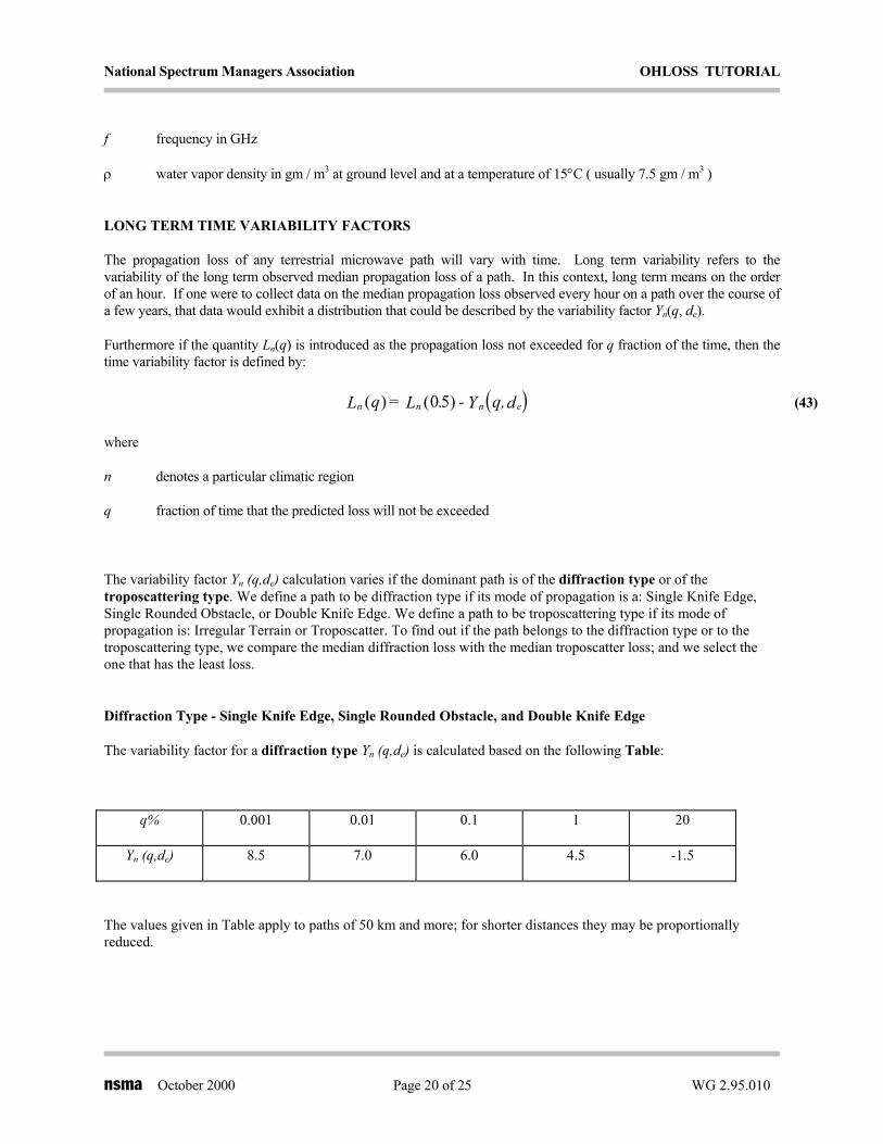
Diffraction Type - Single Knife Edge, Single Rounded Obstacle, and Double Knife Edge

The variability factor for a diffraction type Yn (q,de) is calculated based on the following Table:

q% 0.001 0.01 0.1 1 20

Yn (q,de) 8.5 7.0 6.0 4.5 -1.5

The values given in Table apply to paths of 50 km and more; for shorter distances they may be proportionally reduced.



Troposcattering Type - Irregular Terrain or Troposcatter

The variability factor for a troposcattering type Yn (q,de) is calculated as follows: notice that by definition Yn (0.5,de) is zero. The variability factor Yn (0.1,de) can be calculate for different climatic regions using the general parametric expression given in equation (40) with the constants in Table II. The quantity Ln(0.1) represents the transmission loss which will be exceeded for 90% of the time. In analyzing radio interference, one is concerned with predicted loss values that will be exceeded for percentages of time near 100%, which corresponds to small values of q.

Table II Yn(0.1, de) Evaluation Constants

Region C1 C2 C3 n1 n2 n3 fm f∞

Continental Temperate 1.50e-02 7.40e-06 1.50e-11 1.33 2.10 4.95 13.30 6.10

Maritime Temperate Overland

6.28e-04 3.19e-08 6.06e-12 1.92 2.96 5.05 13.00 12.50

Maritime Temperate Overseas

1.82e-02 2.40e+00 6.92e-15 1.29 0.00 5.78 19.00 14.00

In the continental temperate climatic region, (region number 1), values for other time percentages can be determined by the following multipliers of Y1(0.1, de):

% time loss exceeded q Y1(q, de)

50.0000% 0.5 0.0

80.0000% 0.2 0.6567⋅Y1(0.1, de)

90.0000% 0.1 1.00 ⋅ Y1(0.1, de)

99.0000% 0.01 2.00 ⋅ Y1(0.1, de)

99.9000% 0.001 2.73 ⋅ Y1(0.1, de)

99.9900% 0.0001 3.33 ⋅ Y1(0.1, de)

99.9950% 0.00005 3.45 ⋅ Y1(0.1, de)

99.9975% 0.000025 3.61 ⋅ Y1(0.1, de)

Unfortunately in the other climatic regions there are no simple relationships between Yn(0.1, de) and the other Yn(q, de) values. In these climatic regions one must use the graphs in Tech Note 101[1] to determine the values of Yn(q, de). Figure 10.27 should be used for the maritime overland region and figure 10.28 for the maritime overseas region.



95 Percent Confidence Factor Adjustment

In addition to time variability, propagation paths with similar path parameters can have different median losses. This uncertainty is a result of the limitations of the models used to predict the propagation loss. This variability between different paths with similar parameters tends to follow a log normal distribution with a variance that is a function of q. In order to be 95% confident that the propagation loss on any particular path is at least as large as predicted by Ln(q), then 1.64 standard deviations must be subtracted from Ln(q).

Therefore, the adjustment for a 95 percent confidence level is given by:

L qnn

n− ( )29 10

( ) ( )n n eL q + Y q d− 164 12 73 012 2. . . , (44)

Variability Limitation Referenced to Free Space

Sometimes when computing time variability losses Ln(q), particularly for very small values of q and at a 95% confidence level, these values are negative. This implies that the propagation loss has some probability of being less than the free space loss. Indeed the propagation loss can become less than free space during unusual events such as atmospheric ducting, however it is extremely rare that the loss becomes significantly less than free space. Therefore an adjustment is made to negative time variability losses that limits how quickly they can become less than the free space loss. This adjusted loss is defined as:

L q

L q L q

L qL q

L qn

n n

n′ =

≥

−<

( )

( ); ( )

( )( )

; ( )

0

290

(45)

This free space referenced variability adjustment has been taken from the ITS irregular terrain model[2][3].

TERRAIN DATA BASES

There are various sources for terrain data that may be used as input to the OHLOSS program. The most elementary of these is the extraction of data from topographic maps and manually entering the data into the program. Although this method is time consuming, the resulting terrain profile represents the most accurate representation if small scale maps (1:24,000) are used.

There are several digitized data bases that also may be used. The most crude of these is the 30 second data, which is based on 1:250,000 scale maps. There are data bases of 3 second data, also based on 1:250,000 scale maps. Either of these may be used, but care must be exercised in the use of the output of the program, especially in situations that indicate a marginal loss to resolve interference cases. Several common problems are given below.

• In mountainous regions, the contour interval may be 500 feet on a 1:250,000 scale map. The terrain data base may not provide any additional resolution other than the contour information on these maps and the data assumes a constant elevation over the area of the highest contour. This can result in an elevation error approaching 500 feet on a critical point on the path.

• On paths which are controlled by tropospheric scatter, it is always advisable to verify the elevations at the transmit and receive horizons.



OHLOSS SAMPLE CALCULATIONS

Annex 2 of this tutorial gives a series of profiles which illustrate the concepts described in this tutorial. Calculated results are provided with sufficient detail to permit a comparison of OHLOSS programs in Annex 3.

OHLOSS REPORT FORMAT

A standard OHLOSS report format is proposed to allow a simple comparison of the results produced by various programs. The following format represents an amalgamation of all entries currently used in OHLOSS reports.



Site 1 Site 2

Latitude

Longitude

Bearing (deg)

Elevation AMSL (ft/m)

Antenna Height AGL (ft/m)

Antenna Gain (dB)

Effective Antenna Height (ft/m)

Horizon Distance (mi/km)

Horizon Elevation (ft/m)

Horizon Angle (deg/mr)

Ray Cross Over Angle (deg/mr)

Ray Cross Over Distance (mi/km)

Frequency (MHz)

Polarization

Path Length (mi/km)

Effective Path Length (mi/km)

Terrain Elevation Range (ft/m)

K or Surface Refractivity

Climate Region

Ground Type

Type of Path

Reference Diffraction Loss (dB)

Reference Scatter Loss (dB)

Reference Combined Loss (dB)

Median Combined Loss (dB)

Free Space Loss (dB)

Atmospheric Absorption Loss (dB)

Total Median Loss (dB)




Time Variability

Probability Total Loss Exceeds

% 50% Confidence Factor 95% Confidence Factor

50.0000

80.0000

90.0000

99.9900

99.9950

99.9975

99.9999

Most of the OHLOSS reports provide a listing of the terrain data under the following headings:

• distance

• elevation

• obstruction

• clearance at K = ∞

• clearance at K = 1.33

1 Transmission Loss Predictions for Tropospheric Communication Circuits; P. L. Rice, A. G. Longley, K. A. Norton, A. P. Barsis; NBS Technical Note 101, Revised Vols I and II; U.S. Department of Commerce National Bureau of Standards - National Technical Information Service, Springfield, VA; 1967; Reports AD-687-820 and AD-687-821

2 The ITS Irregular Terrain Model, version 1.2.2 - The Algorithm; G. A. Hufford; National Telecommunications and Information Administration - Institute for Telecommunication Sciences; Boulder, CO; (http://elbert.its.bldrdoc.gov/itm.html)

3 A Guide to the Use of the ITS Irregular Terrain Model in the Area Prediction Mode; G. A. Hufford, A. G. Longley, W. A. Kissick; U.S. Department of Commerce - National Technical Information Service, Springfield, VA; Apr 1982; NTIA Report 82-100 / PB82-217977

OHLOSS ANNEX 1 TUTORIAL

nsma October 2000 A1-1

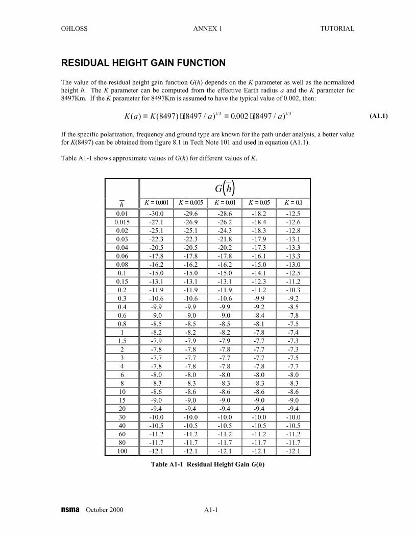
RESIDUAL HEIGHT GAIN FUNCTION

The value of the residual height gain function G(h) depends on the K parameter as well as the normalizedheight h. The K parameter can be computed from the effective Earth radius a and the K parameter for8497Km. If the K parameter for 8497Km is assumed to have the typical value of 0.002, then:

K a K a a( ) ( ) ( / ) . ( / )/ /= ⋅ = ⋅8497 8497 0 002 84971 3 1 3

If the specific polarization, frequency and ground type are known for the path under analysis, a better valuefor K(8497) can be obtained from figure 8.1 in Tech Note 101 and used in equation (A1.1).

Table A1-1 shows approximate values of G(h) for different values of K.

(A1.1)

( )G hh K = 0001. K = 0 005. K = 0 01. K = 0 05. K = 01.

0.01 -30.0 -29.6 -28.6 -18.2 -12.50.015 -27.1 -26.9 -26.2 -18.4 -12.60.02 -25.1 -25.1 -24.3 -18.3 -12.80.03 -22.3 -22.3 -21.8 -17.9 -13.10.04 -20.5 -20.5 -20.2 -17.3 -13.30.06 -17.8 -17.8 -17.8 -16.1 -13.30.08 -16.2 -16.2 -16.2 -15.0 -13.00.1 -15.0 -15.0 -15.0 -14.1 -12.5

0.15 -13.1 -13.1 -13.1 -12.3 -11.20.2 -11.9 -11.9 -11.9 -11.2 -10.30.3 -10.6 -10.6 -10.6 -9.9 -9.20.4 -9.9 -9.9 -9.9 -9.2 -8.50.6 -9.0 -9.0 -9.0 -8.4 -7.80.8 -8.5 -8.5 -8.5 -8.1 -7.51 -8.2 -8.2 -8.2 -7.8 -7.4

1.5 -7.9 -7.9 -7.9 -7.7 -7.32 -7.8 -7.8 -7.8 -7.7 -7.33 -7.7 -7.7 -7.7 -7.7 -7.54 -7.8 -7.8 -7.8 -7.8 -7.76 -8.0 -8.0 -8.0 -8.0 -8.08 -8.3 -8.3 -8.3 -8.3 -8.3

10 -8.6 -8.6 -8.6 -8.6 -8.615 -9.0 -9.0 -9.0 -9.0 -9.020 -9.4 -9.4 -9.4 -9.4 -9.430 -10.0 -10.0 -10.0 -10.0 -10.040 -10.5 -10.5 -10.5 -10.5 -10.560 -11.2 -11.2 -11.2 -11.2 -11.280 -11.7 -11.7 -11.7 -11.7 -11.7

100 -12.1 -12.1 -12.1 -12.1 -12.1

Table A1-1 Residual Height Gain G(h)



Equation (A1.2) along with the co-efficient parameters in Table A1-2 and Table A1-3 can be used tocompute G(h) for certain values of K. This functional representation of G(h) was determined by empiricalcurve fitting and is certainly not the only possible representation of G(h), however it is a reasonablyaccurate approximation. When G(h) is needed for a value of K between those defined in equation (A1.2),the values of G(h) for K less than the desired value and G(h) for K greater than the desired value should becomputed. These two values should then be interpolated to determine the value of G(h) at the desiredvalue of K.

G h

A A h A h A h h

Q Q h Q h Q h Q h h

h h h

h h

( )

log( ) log ( ) log ( ); . .

log( ) log ( ) log ( ) log ( ); . .

log( ) log ( ); .

. . log( );

≈

− − − − ≤ <

− − − − − ≤ <

− − − ≤ <

− − ≤

0 1 22

33

0 1 22

33

44

2

0 01 01

01 6 0

6 0 100

4 9 36 100

6.683294 1.044877 0.8317378

A plot of the curves defined by equation (A1.2) is shown in Figure A1-1 along with values specified inTable A1-1.

(A1.2)

K = 01. K = 0 05. K = 0 01. K = 0 005. K ≤ 0 001.A0

-13.62594 -2.64703 7.260619 11.38374 9.752453

A1-52.92282 -23.07055 -2.109046 7.338009 3.179422

A2-33.66384 -6.323515 6.980349 13.68546 10.20234

A3-6.866956 0.0 1.350013 2.731197 1.775372

Table A1-2 G(h) A Co-efficients

K = 01. K = 0 05. K ≤ 0 01.Q0 7.346936 7.861696 8.24355Q1 -1.3225 -1.75399 -2.534023Q2 4.12942 3.659145 3.375534Q3 -0.8458644 -1.211522 -0.747357Q4 -1.14472 -0.3863533 0.09953648

Table A1-3 G(h) Q Co-efficients



Figure A1-1 Residual Height Gain Function

R e s i d u a l H e i g h t G a i n F u n c t i o n

h

G(

h)

[

dB

]

O . O 1 O . O 2 O . O 5 O . 1 O . 2 O . 5 1 2 5 1 O 2 O 5 O 1 O O

- 3 O

- 2 5

- 2 O

- 1 5

- 1 O

- 5

O



IRREGULAR TERRAIN FUNCTIONS

The F(x,K) Function

Approximate values for F(x,K) are shown in Table A1-4 for various values of x and K. Furthermore, afunctional representation of F(x,K) empirically determined by curve fitting is given by equations (A1.3)and (A1.4). A plot of this functional representation and the tabulated values of F(x,K) is shown in. FigureA1-2.

( )F x K

K xx

xK x

x

G x x x x

( , )

log ;

log log ;

( ) . log( );

≈

+

≤

+ +

< ≤

= − <

1010 10 800

200

1010 10 800

200 2000

0 05751 10 2000

2 4

2 4

∆

where

∆( )z z z z≡ + +-1258.95 1557.105 - 643.3046 88.820852 3

F x K( , )x K = 0 0001. K = 0 001. K = 0 01. K = 01.1 -95.0 -75.0 -55.0 -35.0

1.5 -94.5 -75.0 -55.0 -35.02 -94.0 -75.0 -55.0 -35.03 -93.0 -75.0 -55.0 -35.04 -90.5 -75.0 -55.0 -35.06 -85.0 -74.5 -55.0 -35.08 -80.5 -73.5 -55.0 -35.0

10 -76.0 -72.5 -55.0 -35.015 -69.5 -68.0 -55.0 -35.020 -64.5 -64.0 -54.5 -35.030 -57.5 -57.5 -53.0 -35.040 -52.5 -52.5 -50.5 -34.560 -45.5 -45.5 -45.0 -34.080 -40.5 -40.5 -40.5 -33.5100 -36.5 -36.5 -36.5 -32.0150 -29.5 -29.5 -29.5 -27.5200 -24.0 -24.0 -24.0 -23.0300 -16.5 -16.5 -16.5 -16.0400 -10.0 -10.0 -10.0 -10.0600 1.5 1.5 1.5 1.5800 13.5 13.5 13.5 13.5

1000 25.0 25.0 25.0 25.01500 53.5 53.5 53.5 53.5

Table A1-4 The F(x,K) Function

(A1.3)

(A1.4)



I r r e g u l a r T e r r a i n F ( x )

x

F(

x)

[

dB

]

1 2 5 1 O 2 O 5 O 1 O O 2 O O 5 O O 1 O O O 2 O O O

- 1 O O

- 9 O

- 8 O

- 7 O

- 6 O

- 5 O

- 4 O

- 3 O

- 2 O

- 1 O

O

1 O

2 O

3 O

4 O

5 O

6 O

7 O

Figure A1-2 The Irregular Terrain F(x,K) Function



The C1(K) FunctionApproximate values for C1(K) are shown in Table A1-5 for various values of K. Furthermore, a functionalrepresentation of C1(K) empirically determined by curve fitting is given by equation (A1.5). A plot of thisfunctional representation and the tabulated values of C1(K) is shown in Figure A1-3.

C K

K

. . K K K

K K K

K

1

2

2

20 03 0 01

20 08597 5 63597 39 0 01 1

15 1 100

20 94 100

( )

. ; .

. ; .

. ;

. ;

≈

<

− + ≤ <

− + ≤ <

≤

20.98116 4.131162

K C K b o1 90( ); =

0.01 20.030.02 19.950.03 19.920.04 19.900.06 19.850.08 19.750.1 19.640.2 19.150.3 18.700.4 18.350.6 18.100.8 18.151 18.352 19.303 19.754 20.056 20.308 20.45

10 20.5520 20.7530 20.8040 20.8560 20.8880 20.91

100 20.94

Table A1-5 C1(K) Function

(A1.5)



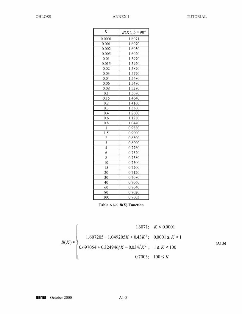
The B(K) Function

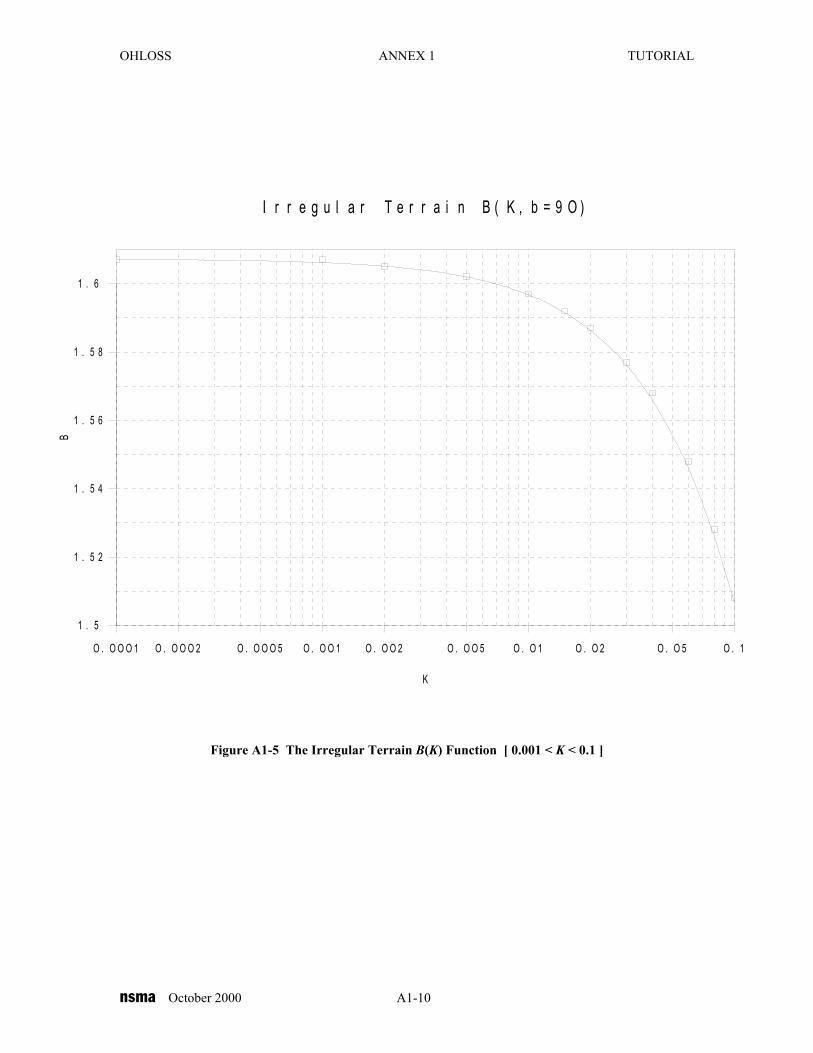
Approximate values for B(K) are shown in Table A1-6 for various values of K. Furthermore, a functionalrepresentation of B(K) empirically determined by curve fitting is given by equation (A1.6). A plot of thisfunctional representation and the tabulated values of B(K) is shown in Figure A1-4 and Figure A1-5.

I r r e g u l a r T e r r a i n C 1 ( K , b = 9 O )

K

C1

[

dB

]

O . O 1 O . O 2 O . O 5 O . 1 O . 2 O . 5 1 2 5 1 O 2 O 5 O 1 O O

1 5

1 6

1 7

1 8

1 9

2 O

2 1

2 2

Figure A1-3 The Irregular Terrain C1(K) Function



B K

K

K K K

. . K K K

K

( )

. ; .

. ; .

. ;

. ;

≈

<

− + ≤ <

+ − ≤ <

≤

16071 0 0001

0 43 0 0001 1

0 697054 0 324946 0 034 1 100

0 7003 100

2

2

1.607205 1.049205

K B K b o( ); = 900.0001 1.60710.001 1.60700.002 1.60500.005 1.60200.01 1.5970

0.015 1.59200.02 1.58700.03 1.57700.04 1.56800.06 1.54800.08 1.52800.1 1.5080

0.15 1.46400.2 1.41600.3 1.33600.4 1.26000.6 1.12800.8 1.04401 0.9880

1.5 0.90002 0.85003 0.80004 0.77606 0.75208 0.7380

10 0.730015 0.720020 0.712030 0.708040 0.706060 0.704080 0.7020

100 0.7003

Table A1-6 B(K) Function

(A1.6)



I r r e g u l a r T e r r a i n B ( K , b = 9 O )

K

B

O . 1 O . 2 O . 5 1 2 5 1 O 2 O 5 O 1 O O

O . 6

O . 7

O . 8

O . 9

1

1 . 1

1 . 2

1 . 3

1 . 4

1 . 5

1 . 6

Figure A1-4 The Irregular Terrain B(K) Function [ 0.1 < K < 100 ]



I r r e g u l a r T e r r a i n B ( K , b = 9 O )

K

B

O . O O O 1 O . O O O 2 O . O O O 5 O . O O 1 O . O O 2 O . O O 5 O . O 1 O . O 2 O . O 5 O . 1

1 . 5

1 . 5 2

1 . 5 4

1 . 5 6

1 . 5 8

1 . 6

Figure A1-5 The Irregular Terrain B(K) Function [ 0.001 < K < 0.1 ]

Documents

Recommendation WG 2.99.052 (Supersedes Rec. WG …nsma.org/wp-content/uploads/2016/05/WG2-99-052.pdf · October 2000 Source: Working Group 2 Recommendation WG 2.99.052 (Supersedes