Receptor modeling of C2–C7 hydrocarbon sources at an urban

Atmos. Chem. Phys., 8, 2313–2332, 2008www.atmos-chem-phys.net/8/2313/2008/© Author(s) 2008. This work is distributed underthe Creative Commons Attribution 3.0 License.

AtmosphericChemistry

and Physics

Receptor modeling of C2–C7 hydrocarbon sources at an urbanbackground site in Zurich, Switzerland: changes between1993–1994 and 2005–2006

V. A. Lanz1, C. Hueglin1, B. Buchmann1, M. Hill 1, R. Locher2, J. Staehelin3, and S. Reimann1

1Empa, Swiss Federal Laboratories for Materials Testing and Research, Laboratory for Air Pollution and EnvironmentalTechnology, 8600 Duebendorf, Switzerland2ZHAW, School of Engineering, Institute of Data Analysis and Process Design IDP, 8401 Winterthur, Switzerland3Institute for Atmospheric and Climate Science, ETH Zurich, 8092 Zurich, Switzerland

Received: 28 November 2007 – Published in Atmos. Chem. Phys. Discuss.: 18 January 2008Revised: 7 April 2008 – Accepted: 14 April 2008 – Published: 5 May 2008

Abstract. Hourly measurements of 13 volatile hydrocar-bons (C2–C7) were performed at an urban background sitein Zurich (Switzerland) in the years 1993–1994 and againin 2005–2006. For the separation of the volatile organiccompounds by gas-chromatography (GC), an identical chro-matographic column was used in both campaigns. Changesin hydrocarbon profiles and source strengths were recoveredby positive matrix factorization (PMF). Eight and six factorscould be related to hydrocarbon sources in 1993–1994 and in2005–2006, respectively. The modeled source profiles wereverified by hydrocarbon profiles reported in the literature.The source strengths were validated by independent mea-surements, such as inorganic trace gases (NOx, CO, SO2),methane (CH4), oxidized hydrocarbons (OVOCs) and mete-orological data (temperature, wind speed etc.). Our analysissuggests that the contribution of most hydrocarbon sources(i.e. road traffic, solvents use and wood burning) decreasedby a factor of about two to three between the early 1990sand 2005–2006. On the other hand, hydrocarbon losses fromnatural gas leakage remained at relatively constant levels(−20%). The estimated emission trends are in line with theresults from different receptor-based approaches reported forother European cities. Their differences to national emissioninventories are discussed.

Correspondence to:V. A. Lanz([email protected])

1 Introduction

Air pollutants can have adverse impacts on human health,most notably on the respiratory system and circulation (Nel,2005), acidify and eutrophicate ecosystems (Matson et al.,2002), diminish agricultural yields, corrode materials andbuildings (Primerano et al., 2000), and decrease atmosphericvisibility (Watson, 2002). Organic gases and particles canboth be directly emitted into the atmosphere, e.g. by fos-sil fuel combustion, or secondarily formed and decomposedthere by chemical reactions and/or gas-to-particle conver-sions (Fuzzi et al., 2006). Volatile organic compounds(VOCs) have several important impacts: while only someof them are toxic to humans, e.g. benzene (WHO, 1993),or relevant greenhouse gases, e.g. methane (Forster et al.,2007), all VOCs are oxidized in the atmosphere and most arethereby involved in the formation of secondary pollutants,such as ozone (O3), and secondary organic aerosol (SOA).Ambient VOC measurements became important since the1950s (Eggertsen and Nelsen, 1958) due to summer smogphenomena, first and foremost due to high O3 levels in theLos Angeles basin. The identification and quantification ofVOC sources is therefore a necessary step to mitigate air pol-lution.

Receptor models were developed to attribute measuredambient air pollutants to their emission sources. Dependingon the degree of prior knowledge of the sources, a chemicalmass balance (CMB; composition of the emission sources isknown), a multivariate receptor model (no a priori knowl-edge) or a hybrid model in between these extreme cases ismost appropriate (Hopke, 1988; Wahlin, 2003; Christensen

Published by Copernicus Publications on behalf of the European Geosciences Union.

http://creativecommons.org/licenses/by/3.0/

2314 V. A. Lanz et al.: Source apportionment of volatile hydrocarbons

Table 1. Mean concentrations and standard deviations [ppb] of the 13 considered hydrocarbon species for the years 2005–2006 (n=8912)and values for 1993–1994 (n=7606) in brackets. Detection limits (DL, in ppt) and the relative measurement error (coefficient of variation,CV) for each hydrocarbon species as used for PMF are also given.∗Ethane and ethyne concentrations in 1993–1994 were partially imputed.∗∗ Please consider the paragraph on nomenclature in Sect. 2.1.1.

species synonym formula mean conc. [ppb] std. dev. [ppb]DL [ppt] CV [rel.]

ethane dimethyl C2H6 2.34 (3.03)∗ 1.32 (2.17) 10 (15) 0.02 (0.05)ethene ethylene C2H4 1.85 (3.03) 1.38 (2.54) 10 (15) 0.02 (0.05)propane n-propane C3H8 1.25 (1.43) 0.87 (0.89) 7 (10) 0.02 (0.05)propene propylene C3H6 0.42 (0.90) 0.32 (0.76) 7 (10) 0.02 (0.05)ethyne acetylene C2H2 1.13 (3.87)∗ 0.74 (3.09) 10 (8) 0.03 (0.05)isobutane 2-methylpropane C4H10 0.59 (0.94) 0.44 (0.72) 5 (8) 0.02 (0.10)butane n-butane C4H10 0.99 (2.76) 0.78 (2.04) 5 (8) 0.03 (0.10)isopentane 2-methylbutane C5H12 1.24 (2.96) 1.02 (2.32) 5 (7) 0.03 (0.10)pentane n-pentane C5H12 0.48 (0.94) 0.35 (0.68) 4 (7) 0.03 (0.10)isohexanes (sum) ∗∗ C6H14 0.86 (1.17) 0.68 (0.96) 3 (7) 0.03 (0.08)hexane n-hexane C6H14 0.13 (0.29) 0.16 (0.23) 3 (6) 0.03 (0.10)benzene benzol C6H6 0.38 (0.95) 0.27 (0.68) 3 (5) 0.03 (0.05)toluene methylbenzene C7H8 1.37 (2.57) 1.15 (2.37) 3 (4) 0.03 (0.05)

et al., 2006). The first multivariate source apportionmentstudies were based on the elemental composition of partic-ulate matter (e.g. Blifford and Meeker, 1967). In contrastto organic species, element concentrations (e.g. of airbornemetals) do not change because of degradation or secondaryformation in the atmosphere. Given that their sources emitthose elements in constant proportions over time, the cal-culated receptor profiles can directly be related to sources.More recently, receptor models have also been applied to or-ganic compounds since detailed chemical information aboutthe organic gas- and aerosol-phase is available (e.g. usinghigh-resolution gas-chromatography, Schauer et al., 1996,or aerosol mass spectrometry, Lanz et al., 2007). However,the fundamental assumption of non-reactivity or mass con-servation (Hopke, 2003) can be violated and the calculatedfactors may not always be directly related to emission pro-files but have to be interpreted as aged profiles (dependingon the selected species and measurement location). There-fore, a flexible model such as positive matrix factorization(PMF; Paatero and Tapper, 1994) is favorable to model VOCconcentration matrices. Furthermore, PMF modeling allowsfor any changes (e.g. local differences) in the nature of theVOC sources. The PMF2 program (Paatero, 1997) uses a sta-ble algorithm to estimate source strengths and profiles frommultivariate data sets (bilinear receptor-model). Miller etal. (2002) concluded for simulated data that PMF was su-perior in recovering VOC sources compared to other recep-tor models based on standard CMB (Winchester and Nifong,1971), principal component analysis (Blifford and Meeker,1967) or UNMIX, a multivariate receptor model developedby Henry (2003). Also Jorquera and Rappengluck (2004)found PMF resolved VOC profiles more reliable than profilesresolved by UNMIX, while Anderson et al. (2002) found the

results of the two models to be in good agreement. Fur-ther evidence that bilinear unmixing by PMF2 can be usedto model VOC data was provided for the Texas area (Buzcuand Frazier, 2006), where for certain emission situations(e.g. wind directional dependencies of point sources etc.) anenhanced PMF was favorable (Zhao et al., 2004).

Due to the environmental problems mentioned above, ab-atement strategies have been developed and implemented forthe reduction of VOC emissions. In fact, the sum of non-methane VOCs at the urban background location in Zurich(Switzerland), as studied in this article, decreased by -50%between 1986 and 1993 and again by -30% from the early1990s to today (Fig. 1). For 1993–1994, about 20 volatilehydrocarbon species were determined at Zurich-Kaserne byhourly resolved gas-chromatography (GC-FID). For 2005–2006, more than 20 hydrocarbons were measured again atthe same site (13 of them were measured during both peri-ods and are summarized in Table 1 and Fig. 2). The samechromatographic column was used for both campaigns. ByPMF modeling of hydrocarbon observations in 1993–1994and in 2005–2006 we describe the underlying factors of eachdata set. The factors recovered by multivariate PMF mod-eling are related to hydrocarbon source profiles and sourcestrengths. This attribution needs to be verified by meansof collocated measurements (inorganic trace gases, oxidizedhydrocarbons, meteorology), by time series analysis of thesource strengths as well as by published VOC profiles andemission factors from the literature. The decrease in ambi-ent VOC concentrations between the early 1990s and today(2005–2006) is explained by comparing the factor analyticalresults for both data sets. The contribution of different emis-sion sources to this trend is discussed.

Atmos. Chem. Phys., 8, 2313–2332, 2008 www.atmos-chem-phys.net/8/2313/2008/

V. A. Lanz et al.: Source apportionment of volatile hydrocarbons 2315


0.40

0.35

0.30

0.25

0.20

0.15

0.10

ppm

C

2005200019951990

t-NMVOC, Zürich-Kaserne (1986-2006)

2005-06

1993-94

Fig. 1. Total concentrations [ppmC] of non-methane volatile or-ganic compounds (t-NMVOC) at an urban background site (Zurich,Switzerland) measured by a standard FID (flame ionization detec-tor). Speciated VOC data is available for 1993–1994 and since 2005(red and blue points).

Fig. 1. Total concentrations [ppmC] of non-methane volatile or-ganic compounds (t-NMVOC) at an urban background site (Zurich,Switzerland) measured by a standard FID (flame ionization detec-tor). Speciated VOC data is available for 1993–1994 and since 2005(red and blue points).

2 Methods

2.1 Measurements

2.1.1 Hydrocarbon measurements

The measurements at Zurich-Kaserne (410 m a.s.l.) are rep-resentative for an urban background site in Zurich, Switzer-land. The sampling site is located in a public backyard nearthe city center. The earlier VOC measurements in 1993–1994were presented by Staehelin et al. (2001). The time spans inthis study included 4 June 1993 to 6 October 1994 and 4 June2005 to 6 October 2006.

18 hydrocarbons were measured quasi-continuously inZurich between 1993 and 1994: first, ambient air waspassed through a Nafion Dryer to minimize its water con-tent and then hydrocarbons were trapped on an adsorption-desorption unit (VOC Air Analyzer, Chrompack) by usinga multi-stage adsorption tube held at−25◦C. The flow ofair through the trap was at 10 ml min−1 and the trappingtime was 30 min, yielding a total volume of 300 ml of sam-pled air. Then the trap was heated to 250◦C for transfer-ring the VOCs to a cryo-focussing trap (PoraPLOT Q), heldat −100◦C. Finally, concentrated VOCs were passed ontothe analytical PLOT column (Al2O3/KCl, 50 m×0.53 mm,Chrompack) by heating to 125◦C. The analysis was per-formed by gas chromatography-flame ionization detection(GC-FID, Chrompack). Calibration was performed regularlyby diluting a commercial standard with zero air to the lowerppb (parts per billion by volume) range.

22 hydrocarbons were measured quasi-continuously in2005–2006: First, ambient air was passed through a NafionDryer to minimize its water content and was then ex-tracted from hydrocarbons using an adsorption-desorptionunit (Perkin-Elmer, TD), equipped with a multi-stage micro-


5

4

3

2

1

0

etha

ne*

ethe

ne

prop

ane

prop

ene

ethy

ne*

isob

utan

e bu

tane

is

open

tane

pe

ntan

e S

-isoh

exan

es

hexa

ne

benz

ene

tolu

ene

1993-1994 2005-2006

ppb

Fig. 2. Averaged values for the 13 hydrocarbons measured in 1993–1994 (red) and in 2005–2006 (blue) at Zurich-Kaserne. *Ethaneand ethyne measurements in 1993–1994 were partially imputed(see text, Sect. 2.2.3). A definition of “S-isohexanes” is given inSect. 2.1.1.

Fig. 2. Averaged values for the 13 hydrocarbons measured in 1993–1994 (red) and in 2005–2006 (blue) at Zurich-Kaserne. *Ethaneand ethyne measurements in 1993–1994 were partially imputed(see text, Sect. 2.2.3). A definition of “S-isohexanes” is given inSect. 2.1.1.

trap held at−30◦C by means of a Peltier element. The flowof air through the trap was 20 ml min−1 and the trapping timewas 15 min, yielding a total volume of 300 ml of sampled air.After flushing with helium to reduce the water vapor contentthe trap was rapidly heated to 260◦C for desorption of thehydrocarbons onto the analytical PLOT column (Al2O3/KCl,50 m×0.53 mm, Varian). The analysis was performed by gaschromatography-flame ionization detection (GC-FID, Agi-lent 6890). Calibrations were performed regularly using astandard which contains the analyzed hydrocarbons in thelower ppb range (National Physical Laboratory, UK).

13 hydrocarbon species were measured in both data sets(summarized in Table 1 and Fig. 2) and used for the statisti-cal analysis. The chromatographic column for separation ofthe VOCs is identical for the two measurement periods. Thisis an advantage for the comparison of the two data sets, al-though newest developments use two-dimensional gas chro-matography (GC×GC) to separate overlapping peaks (e.g.Bartenbach et al., 2007). Trapping efficiency was below100% for the C2 hydrocarbons, which however was correctedby a specific calibration factor.

The hydrocarbon species in this article are named based onIUPAC. As an exception, the term “sum of isohexanes” (S-isohexanes) is used, which refers to the added concentrationsof 2-methylpentane and 3-methylpentane (1993–1994), butfor 2005–2006 the sum includes 2,2-dimethylbutane and 2,3-dimethylbutane as well.

2.1.2 Ancillary data

In addition to the hydrocarbons, about 20 different,hourly resolved OVOCs are available at Zurich-Kaserne for

www.atmos-chem-phys.net/8/2313/2008/ Atmos. Chem. Phys., 8, 2313–2332, 2008


campaigns in summer 2005 and winter 2005/2006. Themeasurements were performed by GC-MS (gas chromato-graph with mass spectrometer) and summarized in Legreid etal. (2007a). Inorganic trace gases (NOx, CO, SO2), meteoro-logical parameters (temperature, wind speed etc.), methane(CH4), and total non-methane VOCs (t-NMVOC) were mea-sured by standard methods (Empa, 2006). Measurements oft-NMVOCs are performed continuously by a flame ioniza-tion detector (FID) (APHA 360, Horiba). For separation be-tween CH4 and t-NMVOCs the air sample is divided into twoparts. One part is directly introduced into the FID, while thesecond part is lead through a catalytic converter to removethe NMVOCs. The outcome of both lines is measured al-ternately and the t-NMVOC concentration is calculated fromthe difference of the two measurements.

2.2 Data analysis and preparation

2.2.1 Unmixing multivariate observations

Linear mixing of observable quantities is the basis to all re-ceptor models and can be represented by the following equa-tion (Henry, 1984):

xi=giF+ei, (1)

wherexi represents thei-th multivariate observation (vec-tor of m variables) and is approximated by linear combi-nations of the loadings or source profiles,F, and scores orsource strengths,gi , up to an error vector,ei . Chemicalmass balance models were designed for estimation of sourcestrengths,gi (a p-dimensional vector), for given numericalvalues ofF, representing ap×m-matrix of the source pro-files, and a specified number of assumed factors or sourcesp.Bilinear receptor models, on the other hand, are most usefulwhen very little or no prior knowledge about the sources isassumed. In such a case, bothgi andF have to be estimated,andp has to be determined by exploratory means. Paateroand Tapper (1994) have proposed to solve Eq. (1) by a least-square algorithm minimizing the uncertainty weighted error(“scaled residuals”):

eij/sij=(xij−yij )/sij , yij=

p∑k=1

gikfkj , (2)

The associated software PMF2 (Paatero, 1997) minimizesthe sum of(eij/sij )

2 (calledQ) for all samplesi=1. . .n andall variablesj=1. . .m. In practice, an enhancedQ is to beminimized, accounting e.g. for penalty terms that ensure anon-negative solution to Eq. (1). This approach implicitlyassumes that uncertainties,sij , for each element of the multi-variate data set,xij , are known. For VOC species, an ad hocmeasurement uncertainty, s

′

ij , has been suggested by Anttilaet al. (1995) and was used in many studies (e.g. Fujita et al.,2003, and Hellen et al., 2006):

s′

ij=

√4(DL)2

j+((CV )jxij )2, (3)

whereDL represents the detection limit (as an absolute con-centration value) and the coefficient of variation,CV, ac-counts for the relative measurement error determined by cal-ibration of the instruments. TheDLs equal five times thebaseline noise of the species’ chromatograms, whereas theCVs are the relative standard deviations of six repeated mea-surements of a real-air standard in the range of ambient con-centrations. Following this method, bothDL and CV arespecies-specific and given in Table 1 for the present hydro-carbon data sets. The total uncertainties,sij , in Eq. (2) cal-culate as

sij=s′

ij+d(max〈xij , yij 〉), (4)

where parameterd symbolizes the relative modeling uncer-tainty andyij the model for xij .

2.2.2 Model specifications and reactivity

For the presented results, the PMF2 program was run withdefault settings (robust mode, central rotation induced byfpeak=0.0, outlier thresholds for the scaled residuals of−4and 4), but the error model (EM=−14) was adjusted for am-bient data. Two-dimensional scatter plots of factor contribu-tions showed edges parallel to the coordinate axes, which isindicating that the chosen rotation has low ambiguity (heuris-tic approach by Paatero et al., 2005). A modeling uncer-taintyd>0% is needed as two basic assumptions about PMFare likely to be violated in this study (constant source pro-files over time and non-reactivity of the species). The resultsshown here were calculated by settingd=10%, which rep-resents an arbitrary but non-critical choice as will be shownbelow. We further assumed that the VOC variability at the ur-ban site Zurich-Kaserne is generally driven by source activi-ties rather than by ageing of the compounds (see Sects. 3.3.2and 3.3.3); VOC transport time from source to receptor wasassumed to be less than 0.5 day on average, which is smallerthan the lifetime of propene, the most reactive compound an-alyzed in the study.

2.2.3 Missing values

In 1993–1994, missing ethane and ethyne concentrationshad to be imputed forn=3450 andn=1500 samples, respec-tively (∼5% of data matrix). These values were missing dueto data acquisition problems. Row-wise deletion of thosemissing values (i.e. a sample is excluded when at least onespecies is not available) would have caused a loss of 50%of the data. We instead have used the k-nearest neighbor(knn) method to estimate those missing values (functionknnof the EMV package in R, The R Foundation for Statisti-cal Computing;www.r-project.org). Additional VOCs wereconsidered for the nearest-neighbor calculations (e.g. 2,2,4-trimethylpentane, 2-methylpropene, and heptane). Advan-tages of data imputation by multivariate nearest neighbormethods in the field of atmospheric research were evaluated


www.r-project.org


by Junninen et al. (2004): they are particularly important forpractical applications as they are fast, perform well, and donot generate new values in the data. We calculated (by repet-itively and randomly assigning missing values to known val-ues) that the relative uncertainty of this imputational methodis about 48% (1σ ) for ethane and about 32% (1σ ) for ethyne.Calculating the uncertainty matrix, the imputed concentra-tion values of ethane and ethyne were multiplied by 0.96(2σ ) and 0.64 (2σ ), respectively, and the square of this prod-uct was added to the error as stated by Eq. (3):

s′

ij=

√4(DL)2

j+(CV )2jx

2ij+(2σxij )2, xij imputed (5)

In summary, this additional term down-weights the imputedvalues by a factor of about 10. Even though the imputedvalues have a minor weight in the minimization algorithmof PMF2, factors characterized by ethane or ethyne for the1993–1994 data should nevertheless be carefully interpreted.

2.2.4 Outliers in the data (contamination-type)

Propane peaks up to 400 ppb (2005–2006) and 200 ppb(1993–1994) could be observed and were most probablycaused by local barbecue events. We have defined extremeobservations to be larger thanµ+σ (2005–2006) andµ+2σ

(1993–1994): About 70 samples were identified and ex-cluded from both data sets in order to not distort the factoranalysis. A detailed inspection of the deleted samples re-vealed that these propane peaks mostly occurred on/beforeweekends and holidays during the summery season, support-ing the hypothesis of local barbecue emissions in the publicbackyard surrounding the measurement site. In 2005–2006,a threshold ofσ rather than 2σ was needed to identify a sim-ilar fraction (∼1%) of outliers. These contamination-typepropane outliers were excluded prior to PMF analysis.

3 Results and discussion

3.1 Determination of the number of factors (p)

The determination of the number of factorsp is a criticalstep for receptor-based source apportionment methods, es-pecially for bilinear models, where very little prior knowl-edge about the sources is assumed. Mathematically perfectmatrix decompositions into scores and loadings do not guar-antee that the solutions are physically meaningful and can beinterpreted. Here, we followed the philosophy that an appro-priate number of factors has to be determined by means ofinterpretability and physical meaningfulness as already pro-posed earlier (e.g. by Li et al., 2004; Buset et al., 2006; Lanzet al., 2007, 2008). Mathematical diagnostics are howeverindispensable to corroborate the chosen solution and to de-scribe the mathematical aspect of its explanatory power.

For the recently (2005–2006) measured VOCs,p=6 fac-tors can be interpreted and are discussed in Sects. 3.4 and 3.5.

Choosing less factors,p<6, coerces two profiles (attributedto “solvent use” and “gasoline evaporation”; see Sect. 3.4).On the other hand, by choosing more factors,p>6, a fac-tor splits from the “gasoline evaporation” factor (the sum oftwo split contributions is very similar,R=0.97, to the gaso-line source contributions retrieved withp=6). We thereforeconsider the 6-factor PMF solution for further analyses ofthe VOC sources in 2005–2006. For the earlier VOC series(1993–1994), we have most confidence in the 8-factor PMFsolution: when assuming 8 factors, for each of the 6 factorsfound in 2005–2006 a similar factor is found as in the ear-lier measurements (plus a toluene source and an additional,combustion-related source). This can not be observed for so-lutions where more than 8 factors or less than 8 factors wereimposed.

The data sets from 1993–1994 and 2005–2006 had tobe described by a different number of factors each (eightand six, respectively) in order to account for the differentemission situations: two factors were absent in the 2005–2006 data, which can be explained by policy regulations (seeSects. 3.5 and 4).

3.2 Mathematical diagnostics

More than 93% and 96% of the variability of the VOCspecies could be explained on average by the 6-factor PMFmodel (2005–2006) and the 8-factor PMF model (1993–1994), respectively (see concept of explained variation;Paatero, 2007). Using the proposed model we can furtherexplain on average 97% and 99% of the total concentrationof the 13 hydrocarbons (in ppb) measured in 2005–2006 and1993–1994, respectively. These latter ratios represent an av-erage modeled to measured hydrocarbon concentration:

ratio = (1/n)

n∑i=1

(

p∑k=1

gik/

m∑j=1

xij ), (6)

wherexij are the observed concentration values,gik repre-sents concentrations modeled byk=1...p factors (note that thefactor profiles were normalized to unity,

∑mj=1 fkj=1), and

n is the number of samples consisting ofm species. Thismeasure is only meaningful, if

∑p

k=1 gik−∑m

j=1 xij≤0 isapproximately fulfilled for virtually all samples and if thereis little scatter in the data, which is the case here. We addi-tionally calculated theR2 of the linear regression,lm, dataversus modeled values

lm(

m∑j=1

xij ∼

p∑k=1

gik), (7)

yielding R2=0.99 in both cases (2005–2006 and 1993–1994,respectively). Thus, almost all variance in the total concen-tration of the 13 hydrocarbons can be explained by the PMFbased model.

For both models, less than 1% of all data points (about100 000 for both data sets) exceeded the model outlier



thresholds for the scaled residuals,|eij/sij |>4, and weredown-weighted (Sect. 2.2). TheQ-value, the total sum ofscaled residuals, equals 11 275 in the robust-mode for the1993–1994 data (n=7606, p=8). For 2005–2006 (n=8912,p=6), this value is 70 018. Thus, for both data sets the calcu-latedQ is in the order of the expectedQ, estimated bymn-p(m+n) as a rule of thumb: The value ofQ should approx-imately equal the degrees of freedoms (e.g. Li et al., 2004),which can be estimated by the number of independent ob-servations,mn, minus the number of estimated parameters,p(m+n). The scaled residuals for each species and both datasets are approximately normally distributedN(0, σj ).

3.3 Robustness of the PMF-solutions

3.3.1 Hydrocarbon species

In order to test the robustness of the presented results, wemade additional PMF runs with 21 hydrocarbons availablesince 2005 (the sum of butenes was deleted column-wisefrom the data matrix due to its abundant missing values).Isoprene and 1,3-butadiene were found to determine two ad-ditional factors almost alone due to their distinct temporalbehavior in ambient air: both VOCs are rapidly removed byradical reactions. Their atmospheric lifetime is in the order ofminutes to hours and these compounds therefore change thevariability structure of the data matrix. However, isopreneand 1,3-butadiene accounted for less than 1% of the total con-centration (in ppb) given by the 22 hydrocarbons retrievedsince 2005 at Zurich-Kaserne. Therefore, the exclusion ofthese latter compounds does not influence the representative-ness, but leads to more robust results. On the other side,aromatic C8 hydrocarbons (m/p-xylene, o-xylene, and ethyl-benzene), which were highly correlated (R>0.97), summedup to considerable concentrations, but did not alter the vari-ability pattern in the data (see Sect. 3.5.1).

3.3.2 Reactivity and modeling uncertainty

Following the idea of Latella et al. (2005), photochemicallyreactive compoundsj can be down-weighted depending on[Ox]l , the oxidant level (i.e. number concentrations of OH,O3, Cl and NO3 radicals), individual rate constants,kj,l

[cm3 molec−1 s−1], and photochemical age,t [s], resultingin a vectorrj

rj = e−t∑

l ([Ox]lkj,l), (8)

which incorporates in the total uncertainty estimates (seeEq. 4) as follows

sij=s′

ij r−1j +d(max〈xij , yij 〉). (9)

Note that for measurements close to sources (t is small) orinert species (kj,l is small), this vector isrj≈1 and Eq. (9)simplifies to the uncertainty model postulated earlier (Eq. 4;

e.g. Lee et al., 1999). The correction factors for the hydr-carbon reactivity (Eq. 8; sticking to the idea of Latella et al.,2005) were calculated assuming an average transport timefrom source to receptor oft=4 h and a typical OH radicalconcentration of 0.8×106 molec cm−3 (Seinfeld and Pandis,1998). The rate constants were derived from Atkinson andArey (2003). The correction factors inr j in the case of theZurich-Kaserne site lie between 0.89 and 1.00 (except forpropene, where a factor of 0.66 has been calculated). Di-viding the analytical uncertainty (Eq. 3) by these correctionfactors and allowing a modeling uncertainty of 10% yieldschanges in the relative mean SCEs (source contribution esti-mates) that are smaller than 1% for each factor in 2005–2006and less than 4% for the factors in 1993–1994. In fact, inthe earlier Zurich data the strongest trend (+3.98%) in therelative mean SCEs can be observed for the “fuel combus-tion” source (factor 6), as its loading of propene (clearly themost reactive compound in our study) was almost as high asethene (the highest peak in factor 6). This is different for the2005–2006 data, where the propene loading in factor 6 ac-counted only half of the ethene intensity. Finally, it shouldbe pointed out that the calculated profiles for the receptor siteZurich-Kaserne could be directly related to measured sourceprofiles from the literature (Sect. 3.4). Thus, the assump-tion that the typical transport time from source to receptoris smaller than the atmospheric lifetime of the most reactivespecies (Sect. 2.2.2) seems to be justified. As shown for or-ganic aerosols (Lanz et al., 2007), it can actually be mean-ingful to interpret PMF factors as secondary and differentlyaged profiles. The same could hold true for more volatileorganics (VOCs) as well, but was not necessary here as wemeasured close to the VOC emission sources (and the chosensubstances are not formed secondarily in the atmosphere).

Generally, the PMF solutions of the presented data werefound to be stable with respect to different uncertainty spec-ifications. In particular, the SCEs are rather insensitive todifferent modeling uncertainties,d. This can be shown byincreasingd from 5% up to 35%, whiler j is kept fixed atunity: For the recent Zurich data (2005–2006), the largestchange due to increasing the modeling uncertainty from 5%to 35% is observed for the relative mean SCEs of factor 2,namely−2.6%. For the earlier data, the SCEs are not verysensitive to modeling uncertainties neither: in analogy to thecase described above, the largest change can be observed forfactor 4 (1993–1994), namely +5.6%. Note that factor 4 isdominated by ethane (and ethyne), both of which were par-tially imputed. It is plausible that imputed species are moresensitive to increases ofd, as the case discrimination in un-certainty levels for missing (Eq. 5) and available data points(Eq. 3) relative to their total uncertainty estimates is down-weighted.




0.25

0.20

0.15

0.10

0.050.00

0.30

0.20

0.10

0.00

0.4

0.3

0.2

0.1

0.0

0.6

0.4

0.2

0.0

0.30

0.20

0.10

0.30

0.20

0.10

0.00

etha

ne

ethe

ne

prop

ane

prop

ene

ethy

ne

isob

utan

e

n-bu

tane

isop

enta

ne

n-pe

ntan

e

S-is

ohex

anes

n-he

xane

benz

ene

tolu

ene

factor 1 ("gasoline evaporation")

factor 2 ("solvents")

factor 3 ("propane")

factor 4 ("ethane")

factor 5 ("wood burning")

factor 6 ("fuel combustion")

PMF factors (2005-06)

Fig. 3. The profiles of the 6-factor PMF solution calculated for therecently measured hydrocarbon data (2005–2006). Each profile’sloadings were normalized to a sum of unity. Here, S-isohexanescomprises 2-methylpentane, 3-methylpentane, 2,2-dimethylbutane,and 2,3-dimethylbutane.

Fig. 3. The profiles of the 6-factor PMF solution calculated for therecently measured hydrocarbon data (2005–2006). Each profile’sloadings were normalized to a sum of unity. Here, S-isohexanescomprises 2-methylpentane, 3-methylpentane, 2,2-dimethylbutane,and 2,3-dimethylbutane.

3.3.3 Down-mixing of aged air masses

An aged profile was determined by averaging gas-phase mea-surements at a rural site (Rigi-Seebodenalp, 1031 m a.s.l.,40 km Southeast of Zurich) during a week-long high-pressure episode in 2005. This profile was fixed and im-posed on the factor analytical solution for the urban data fromZurich-Kaserne (410 m a.s.l.) spanning the same time inter-val.

While the aged profile was frozen during the iterative (hy-brid) model fit, n=1, 2, . . . factors were allowed to evolvefreely within a non-negative subspace. The computationswere carried out using the multilinear engine program, ME-2, designed by Paatero (1999). We have lately described thetechnical details of such an approach (Lanz et al., 2008). Theresulting scores of the imposed profile (enriched with sta-ble and secondary species) did however not show the typical,strong increase during early morning hours as expected forchemically stable and secondary pollutants. Such increases


0.60.40.20.0

0.60.50.40.30.20.10.0

0.200.150.100.050.00

0.6

0.4

0.2

0.0

0.4

0.3

0.2

0.1

0.0

0.30

0.20

0.10

0.00

etha

ne

ethe

ne

prop

ane

prop

ene

ethy

ne

isob

utan

e

n-bu

tane

isop

enta

ne

n-pe

ntan

e

S-is

ohex

anes

n-he

xane

benz

ene

tolu

ene

0.4

0.3

0.2

0.1

0.0

0.250.200.150.100.050.00

factor 4 ("ethane")

factor 3 ("propane")

factor 6 ("fuel combustion")

factor 5 ("wood burning")

factor 1 ("gasoline evaporation")

factor 7 ("earlier traffic source")

factor 2a ("non-toluene solvents")

factor 2b ("toluene")

PMF factors (1993-94)

Fig. 4. The profiles of the 8-factor PMF solution calculated for theearlier hydrocarbon data (1993–1994). Each profile’s loadings werenormalized to a sum of unity. Here, S-isohexanes equals the sum of2-methylpentane and 3-methylpentane.

Fig. 4. The profiles of the 8-factor PMF solution calculated for theearlier hydrocarbon data (1993–1994). Each profile’s loadings werenormalized to a sum of unity. Here, S-isohexanes equals the sum of2-methylpentane and 3-methylpentane.

were ascribed to vertical down-mixing of air from the noctur-nal residual layer to the surface air of the planetary boundarylayer (e.g. McKendry et al., 1997). We therefore concludedthat highly aged and processed air masses do not signifi-cantly influence the variability in the VOC profiles studiedat Zurich-Kaserne.

3.4 Hydrocarbon profiles

In this section, the factor profiles as retrieved by PMF for1993–1994 and 2005–2006 are summarized (Table 2) anddiscussed. We introduce a tentative attribution of PMF fac-tors to emission sources based on a priori knowledge suchas published source profiles. The factors underlying the re-cent measurements (Fig. 3) and the ones explaining the ear-lier VOC data (Fig. 4) are compared with each other, withreference profiles found in the literature, and with profilesreported in Staehelin et al. (2001).

The factors for the recent data (2005–2006) were sorted onthe basis of explained variance (Paatero, 2007). The factors



Table 2. Comparison of the 8-factor PMF (1993–1994 data) with the 6-factor PMF solution for 2005–2006. A total of 13 hydrocar-bons (n=13) were considered for the PMF analysis. The comparison is based on the correlation coefficient: 0.7≤R<0.8, 0.8≤R<0.9, and0.9≤R≤1.0.

PMF factors 1993–1994

fact

or1

(“ga

solin

eev

apor

atio

n”)

fact

or2a

(“no

n-to

luen

eso

lven

ts”)

fact

or2b

(“to

luen

e”)

fact

or3

(“pr

opan

e”)

fact

or4

(“et

hane

”)

fact

or5

(“w

ood

burn

ing”

)

fact

or6

(“fu

elco

mbu

stio

n”)

fact

or7

(“ea

rlier

traf

ficso

urce

”)

factor 1 (“gasoline evaporation”) 0.92 0.38 −0.14 −0.20 −0.16 −0.20 −0.31 0.71factor 2 (“solvents”) 0.42 0.78 −0.20 −0.14 −0.22 −0.21 −0.20 0.34

2005

–200

6P

MF

fact

ors

factor 3 (“propane”) 0.13 −0.40 −0.14 0.94 0.03 −0.08 −0.08 −0.16factor 4 (“ethane”) −0.15 −0.27 −0.06 0.10 0.94 −0.05 0.17 −0.17factor 5 (“wood burning”) −0.28 −0.19 −0.13 −0.09 0.22 0.97 0.43 0.10factor 6 (“fuel combustion”) −0.24 −0.28 0.12 −0.09 −0.25 0.42 0.90 −0.36

calculated for the earlier data (1993–1994) were rearrangedaccording to the order of the factors retrieved from the recentdata (2005–2006).

3.4.1 Profiles for the years 2005–2006

The variability described by factor 1 is dominated by con-tributions of (iso-)pentane, S-isohexanes, (iso-)butane andit includes toluene and benzene (Fig. 3). This feature isshared by gasoline evaporation as well as gasoline combus-tion as can be deduced from the VOC profiles reported inTheloke and Friedrich (2007). In fact, the first PMF com-puted factor correlates well with the following reference pro-files found therein: two-stroke engine, urban mode, warmphase (R=0.94,n=13,n: number of individual hydrocarbons)and cold start phase (R=0.94,n=13) as well as with gasolineevaporation (R=0.97, n=7). Thus, based on its fingerprintalone factor 1 could be related to gasoline combustion and/orgasoline evaporation. A more specific interpretation of thisfirst factor is given in Sect. 3.5.1.

In factor 2, prominent toluene, S-isohexanes and isopen-tane contributions can be observed and most of the toluene(61%), S-isohexanes (52%), hexane (48%), pentane (40%)and isopentane (40%) variability is explained by the secondfactor. This factor is only weakly influenced by the variabil-ity of combustion related C2–C4 hydrocarbons (<10%). Wetherefore attribute this factor to solvent use.

Given the hydrocarbon fingerprint only, factor 3 (propaneand butane) and factor 4 (ethane) could be related to manydifferent sources (natural gas distribution and/or combustion,gas grill emissions, petrol gas vehicles, propellants etc.). Be-cause benzene and toluene do not influence this third fac-tor, we tend to attribute these factors to gas leakage or a

“clean” combustion source. Furthermore, factor 4 is domi-nated by ethane and potentially could also represent an agedbackground profile; ethane is the longest lived species con-sidered in this study. In the Northern Hemisphere, ethaneand propane are principally related to natural gas exploita-tion (Borbon et al., 2004), but the presence of backgroundethane needs to be considered as well. Additional analysesof the source strengths are necessary for further interpreta-tions (Sect. 3.5.3).

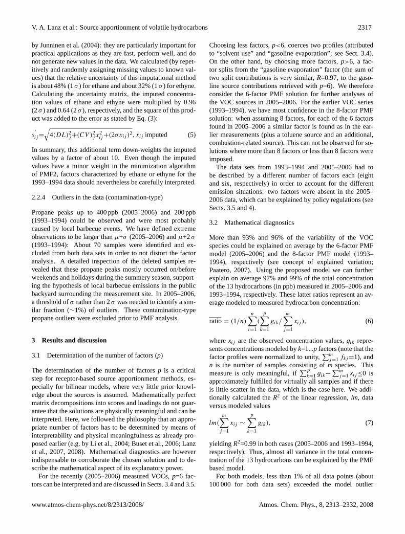
The hydrocarbon profile of factor 5 is similar to a woodburning profile from a flaming stove fire, which is character-ized by ethene and ethyne as can be derived from Barreforsand Petersson (1995) (Fig. 5). Further, factor 5 is also corre-lated (R=0.75,n=9) with the one reference profile for woodcombustion provided in Theloke and Friedrich (2007). Ac-cording to both studies, more benzene than toluene is emit-ted by wood fires ranging from 3:1 ppb/ppb to 8:1 ppb/ppb.This latter value is close to a ratio of 6:1 ppb/ppb in factor 5(2005–2006). Further, the sum of isohexanes is enhanced infactor 5, which is possibly due to furan derivates. Furan is re-leased by wood smoke (Olsson, 2006). Note that the isohex-anes measured in 1993–1994 only included 2-methylpentaneand 3-methylpentane, which are not likely to interfere withfuran derivates. This would explain the absence of the sumof isohexanes in the wood burning profile computed for theancient data (Fig. 4). All these findings suggest that factor 5can be related to wood burning.

Factor 6 is closest (R=0.82, n=13) to the profile mea-sured for diesel vehicles in the urban mode and warm phasewithin the database compiled by Theloke and Friedrich(2007; source profiles representing 87 different anthro-pogenic emission categories in Europe). As observed for



Table 3. Comparison of the 8-factor PMF (1993–1994 data) with factors reported in literature (Staehelin et al., 2001). A total of 12hydrocarbons (n=12) were considered in both studies. The comparison is based on the correlation coefficient: 0.7≤R<0.8, 0.8≤R<0.9, and0.9≤R≤1.0.

PMF factors 1993–1994

fact

or1

(“ga

solin

eev

apor

atio

n”)

fact

or2a

(“no

n-to

luen

eso

lven

ts”)

fact

or2b

(“to

luen

e”)

fact

or3

(“pr

opan

e”)

fact

or4

(“et

hane

”)

fact

or5

(“w

ood

burn

ing”

)

fact

or6

(“fu

elco

mbu

stio

n”)

fact

or7

(“ea

rlier

traf

ficso

urce

”)

factor 1 (“Comb”) −0.10 −0.22 −0.07 −0.15 0.61 0.97 0.51 0.24factor 2 (“Evap”) 0.95 0.39 −0.12 −0.18 −0.02 −0.2 −0.25 0.77

1993

–199

4S

taeh

elin

etal

.

factor 3 (“SO2”) 0.16 −0.48 0.01 0.29 0.86 0.74 −0.03 0.32factor 4 (“Tol”) −0.05 0.00 0.97 −0.16 −0.19 −0.13 0.06 −0.03factor 5 (“NM”) 0.29 −0.06 0.02 0.00 0.84 0.40 −0.28 0.73factor 6 (“Pr”) −0.16 −0.31 0.07 0.99 −0.02 −0.13 0.09 −0.23

wood fires, gasoline and diesel powered vehicles typicallyrelease more alkenes than alkanes as well, but the lattersources emit more toluene than benzene (Staehelin et al.,1998). Increasing toluene-to-benzene ratios during the lastdecade can be derived from emission factors as calculatedfrom a nearby tunnel study: while this ratio was 16:10[mg km−1/mg km−1] in 1993 (Staehelin et al., 1998), a ra-tio of 5:2 [mg km−1/mg km−1] was reported for the year2004 (Legreid et al., 2007a). Let both species be emittedinto an air volume of unity at a distance of unity: we thencan also say that the ratio toluene:benzene increased fromabout 1:1 ppb/ppb to 2:1 ppb/ppb from the early 1990s un-til today. This change is perfectly represented by factor 6(comp. 1993–1994 vs. 2005–2006) and has been caused byrestriction of benzene content in car fuel. The large ratioisopentane-to-pentane as found in factor 6 (namely 10:1) isshared with diesel reference profiles, where a ratio up to 7:1can be calculated (Theloke and Friedrich, 2007). All in all,we interpret factor 6 as fuel combustion with significant con-tributions from diesel vehicles.

3.4.2 Profiles for the years 1993–1994

In this section, the PMF retrieved hydrocarbon profiles fromthe 1993–1994 data are compared first with the factors forthe recently measured data (2005–2006). Then, our PMFsolution for the earlier data is compared to the factors analyt-ical results of a precedent study carried out by Staehelin etal. (2001).

Comparison with recent data (2005–2006)

Five very similar factors (R>0.90,n=13) as found for 2005–2006 (Sect. 3.4.1) can be recovered from the 1993–1994 data(both data sets analyzed by bilinear PMF2). Based on thecorrelation coefficient,R, factors 2a, 2b, and 7 seem to bemissing in the recent data (2005–2006) and the most dra-matic change can be observed for the organic solvents thatwere separated in the earlier data (1993–1994; representedby factor 2a and factor 2b) (Table 2 and Fig. 4).

In 1993, toluene showed a different temporal variabilitythan the other potential organic solvents (isopentane, pen-tane, S-isohexanes, and hexane) and emerges as a distinctfactor. Both factor 2a and 2b virtually only explain the vari-ability of potential solvents (Fig. 6). The distinct temporalbehavior of toluene (with increased concentrations at night)is probably due to the local printing industry that was ac-tive in the 1990s but was not continued after or uses othersolvents. Also Staehelin et al. (2001) identified a distincttoluene source (see Sect. 3.5). It is possible that asphaltworks are represented by factor 2b as well. The addition offactor 2a and 2b (1993–1994) however yields a factor withsimilar loading proportions of toluene, S-isohexanes andisopentanes as found for solvents in the recent data (2005–2006).

In terms ofR, factor 7 is closest to two stroke-engines(R=0.74,n=13) within the reference data base provided byTheloke and Friedrich (2007). However, relatively promi-nent ethyne and S-isohexanes contributions (compared withother types of engines found in Theloke and Friedrich, 2007)point to gasoline driven vehicles without catalytic convert-ers, which still accounted for about 30% of the Swiss fleet in1993–1994 (Staehelin et al., 1998).



Table 4. Correlation of measured trace gases (NOx, CO, CH4, and SO2) and total non-methane VOC, (t-NMVOC), with the PMF calculatedfactors for 2005–2006 (n∼8900 samples) and 1994–1995 (n∼7600 samples). 0.7≤R<0.8, 0.8≤R<0.9, and 0.9≤R≤1.0.

NOx CO SO2 CH4 t-NMVOC

PMF factors 2005–2006factor 1 (“gasoline evaporation”) 0.64 0.63 0.24 0.39 0.72factor 2 (“solvents”) 0.69 0.64 0.22 0.47 0.80factor 3 (“propane”) 0.75 0.77 0.67 0.67 0.65factor 4 (“ethane”) 0.29 0.42 0.54 0.46 0.21factor 5 (“wood burning”) 0.66 0.80 0.58 0.64 0.56factor 6 (“fuel combustion”) 0.76 0.84 0.59 0.53 0.71

PMF factors 1993–1994factor 1 (“gasoline evaporation”) 0.55 0.58 0.32 0.32 0.65factor 2a (“non-toluene solvents”) 0.71 0.76 0.45 0.45 0.77factor 2b (“toluene”) 0.67 0.64 0.44 0.43 0.73factor 3 (“propane”) 0.59 0.54 0.60 0.64 0.45factor 4 (“ethane”) 0.64 0.64 0.72 0.60 0.42factor 5 (“wood burning”) 0.87 0.89 0.75 0.64 0.71factor 6 (“fuel combustion”) 0.88 0.91 0.64 0.58 0.83factor 7 (“earlier traffic source”) 0.61 0.66 0.28 0.31 0.76

Comparison to Staehelin et al. (2001)

Staehelin et al. (2001) also analyzed the Zurich-Kaserne1993–1994 data by non-negatively constraint matrix factor-ization. All six factors mentioned therein correlate well(R>0.80, n=12) with the PMF computed profiles for the1993–1994 data (Table 3). Sources dominated by singleVOC species (toluene and propane source) are here also rep-resented by one single PMF factor. The relation of the otherfactors is however more ambiguous, but for the reasons dis-cussed below it can not be expected that the results of the twostudies are in perfect agreement:

Unlike PMF2, the algorithm used in the precedent studywas based on alternating regression. Similar to the consid-erations by Henry (2003), it was also assumed by Staehe-lin et al. (2001) that the VOC sources can be identified bythe geometrical implications of the receptor model Eq. (1),i.e. there are samples in the data matrix that represent single-source emissions, defining the vertices of the solution spaceprojected onto a plane (and thereby providing starting pointsfor the unmixing algorithm). Contrary to this proceeding, thePMF2 algorithm is started from random initial values by de-fault. In contrast to the present study, Staehelin et al. (2001)included inorganic gases and t-NMVOC in the data matrix.By expanding the data matrix its variability structure was al-tered and factors dominated by inorganic SO2 and NOx aswell as t-NMVOC were identified. Different sources mayhave been coerced as e.g. SO2 is emitted by several sourcetypes (wood burning, diesel fuel combustion etc.), and as ac-tivities of non-SO2 emitting sources can be correlated withthe SO2 time series by coincidence or due to strong meteo-rological influence. Instead, we suggest using the inorganic

gases and sum parameters (t-NMVOC) as independent trac-ers to validate our factor interpretation. Furthermore, woodburning was not considered as potentially important emissionsource by Staehelin et al. (2001).

3.5 Source activities

In this section, the hydrocarbon factors are attributed to emis-sion sources based on comparisons with other, indicativecompounds and meteorological data measured at the samesite. Before the factors are discussed individually, we willfirst give a brief overview of the correlation of computedsource activities with independently measured trace gases atthe same location. The correlation coefficients are summa-rized in Table 4. A positive correlation between a hydrocar-bon and a trace gas can occur because they were emitted bythe same source or because they were released by differentsources showing similar time evolution (e.g. as both may re-flect human activities). However, an evaporative source, asan example, may also be correlated with tracers of combus-tion (e.g. NOx) by coincidence; this clearly impairs the ex-planatory power of interpretations that are exclusively basedon correlation.

Most evident is the high correlation of both the fuel com-bustion and wood burning factor with both nitrogen oxides(NOx) and carbon monoxide (CO) found for both data sets(1993–1994 and 2005–2006). The factor interpreted as gaso-line evaporation shows higher correlations with t-NMVOCthan with combustion tracers, supporting that factor 1 repre-sents a non-combustion source. Also factors that have beenassociated mainly with solvent use (factor 2 in 2005–2006;factors 2a and 2b in 1993–1994, see Sect. 3.4) are more




25

20

15

10

5

0

etha

ne

ethe

ne

prop

ane

prop

ene

ethy

ne

isob

utan

e

buta

ne

pent

ane

hexa

ne

benz

ene

tolu

ene

flaming stove fire (Barrefors and Petersson, 1995)

0.35

0.30

0.25

0.20

0.15

0.10

0.05

"wood burning" factor, Zurich 2005-06 (calculated, PMF)

0.4

0.3

0.2

0.1

0.0

"wood burning" factor, Zurich 1993-94 (calculated, PMF)

Fig. 5. Wood burning profiles calculated by PMF (1993–1994,2005–2006) and from the literature (Barrefors and Petersson, 1995).The PMF loadings are normalized to unity. The measured profilesare given in % volume of total VOC (no isohexanes were deter-mined).

Fig. 5. Wood burning profiles calculated by PMF (1993–1994,2005–2006) and from the literature (Barrefors and Petersson, 1995).The PMF loadings are normalized to unity. The measured profilesare given in % volume of total VOC (no isohexanes were deter-mined).

strongly correlated with t-NMVOC than with the combustiontracers CO, NOx, and SO2. The factors dominated by ethane(factor 4) show activities that are closest to sulphur dioxide(SO2), which may point to a source active in winter, com-bustion of sulphur-rich fuel or long-range transport. Methane(CH4) is strongest correlated with the “propane” factors; thisdiscussion will be continued in more detail (Sect. 3.5.3).

3.5.1 Traffic-related sources

Gasoline evaporation

Modeled gasoline evaporation sources (factor 1) in 1993–1994 and in 2005–2006 are positively correlated with tem-peratureR=0.45 andR=0.30 (Fig. 7), respectively, whilethe other factors (related to road traffic) show a different sea-sonal behavior, typically anti- or uncorrelated with temper-ature. In several cases, positive deviations from the linearregression slope (scores vs. temperature) coincide with lowwind speed (Fig. 7), which is indicative for thermal inver-


100

80

60

40

20

0

etha

ne

ethe

ne

prop

ane

prop

ene

ethy

ne

isob

utan

e

n-bu

tane

isop

enta

ne

n-pe

ntan

e

S-is

ohex

anes

n-he

xane

benz

ene

tolu

ene

non-solvents potential organic solvents

Explained variance [%] by factor 2a and factor 2b (1993-1994)

Fig. 6. Explained variance by factor 2a (“non-toluene solvents”)and factor 2b (“toluene”) for the 13 hydrocarbons considered forthis study. Non-solvents comprise C2–C4 hydrocarbons ethane,ethene, propane, propene, ethyne, isobutene and butane. C5–C7 hy-drocrabons isopentane, n-pentane, S-isohexanes, n-hexane, benzeneand toluene are potential organic solvents. S-isohexanes includes 2-methylpentane and 3-methylpentane

Fig. 6. Explained variance by factor 2a (“non-toluene solvents”)and factor 2b (“toluene”) for the 13 hydrocarbons considered forthis study. Non-solvents comprise C2–C4 hydrocarbons ethane,ethene, propane, propene, ethyne, isobutene and butane. C5–C7 hy-drocrabons isopentane, n-pentane, S-isohexanes, n-hexane, benzeneand toluene are potential organic solvents. S-isohexanes includes 2-methylpentane and 3-methylpentane

sions and pollutant accumulation (e.g. in February 1994, Oc-tober 2005, and November 2005). This general dependencesuggests that factor 1 in both data sets represents gasoline re-lease via evaporation, during cold starts and re-fueling ratherthan by warm-phase combustion. A positive correlation withtemperature might also be due to a combustion-related gaso-line source that is active in summer (e.g. from ship traffic orfrom engines used at road works), but is rather unlikely dueto relatively low correlations with the inorganic combustiontracers (Table 4).

The comparison of the PMF calculated gasoline factorwith methyl-tert-buthyl-ether (MTBE) measured during twocampaigns in 2005–2006 (Legreid et al., 2007b) providesfurther evidence for an evaporative gasoline loss. Poulopou-los and Philippopoulos (2000) reported MTBE exhaust emis-sion particularly during cold start and from evaporation. Thisis in agreement with other studies (e.g. MEF, 2001). Further,MTBE is neither synthesized in Switzerland nor formed sec-ondarily in the atmosphere, but exclusively used as a gaso-line additive with concentrations between 2% and 8% pervolume (BAFU, 2002). The gasoline factor is strongly corre-lated with MTBE in summer as well as in winter (Fig. 8) and,therefore, likely represents evaporative gasoline loss and coldstart phases. The slightly higher correlation found in sum-mer (R=0.81) compared to winter (R=0.71) is most probablydue to larger temperature differences between day and night,which determine the amplitude of evaporative gasoline loss.

Gasoline and diesel fuel combustion

As for gasoline evaporation, factors representing fuel com-bustion were also found in both data sets (factor 6). They ex-hibit a bimodal daily cycle with peaks in the morning around




5

4

3

2

1

020151050

3.02.82.62.42.22.01.8

wind speed, m

/s

February 1994

factor 1 ("gasoline evaporation"), 1993-94

temperature

R = 0.45

ppb

3.0

2.0

1.0

0.020151050

October 2005

March 2006

R = 0.30

factor 1 ("gasoline evaporation"), 2005-06

temperature

November 2005

ppb

2.4

2.2

2.0

1.8

1.6

wind speed, m

/s

Fig. 7. Monthly median scores of the gasoline factors (PMF re-trieved), temperature and wind speed for the years 1993–1994 (bot-tom) and 2005–2006 (top). Positive deviations from the regres-sion slope scores vs. temperature represent months characterizedby frequent thermal inversions: February 1994, October 2005,and January 2006. Regression slopes (coefficient value ± 1σ):0.043±0.027 (1993–94, n=12) and 0.018±0.018 (2005-06, n=12)for the monthly values presented above, 0.116±0.006 (1993–94,n=7606) and 0.032±0.002 (2005–06, n=8912) for all data points.

Fig. 7. Monthly median scores of the gasoline factors (PMF re-trieved), temperature and wind speed for the years 1993–1994(bottom) and 2005–2006 (top). Positive deviations from theregression slope vs. temperature represent months characterizedby frequent thermal inversions: February 1994, October 2005,and January 2006. Regression slopes (coefficient value±1σ ):0.043±0.027 (1993–1994,n=12) and 0.018±0.018 (2005–2006,n=12) for the monthly values presented above, 0.116±0.006 (1993–1994,n=7606) and 0.032±0.002 (2005–2006,n=8912) for all datapoints.

07:00 a.m. and in the evening at 09:00 p.m. in both data sets,as shown in Fig. 9 for the recent case (2005–2006). Typ-ically, this temporal behavior is much more prominent onworking days. A very similar pattern as found here wasalso reported for organic aerosol emissions from incompletefuel combustion and NOx at Zurich-Kaserne (Lanz et al.,2007). The pronounced diurnal variation of this factor duringweekdays indicates that other fossil fuel combustion sources(e.g., off-road vehicles and machines) have a minor impor-tance at this site. On the other hand, the strong dependenceof the day of the week further supports findings based onthe hydrocarbon fingerprint of this factor (Sect. 3.4), namelythat diesel exhaust is a major contributor. A large fraction(∼66%, deduced from BAFU, 2000) of diesel-related totalhydrocarbons in 2000 was caused by the heavy-duty fleet(transport of goods), which is not allowed to drive on week-ends in Switzerland. Also commuter traffic is at a minimum,but the share of diesel passenger cars was and is still com-paratively low in Switzerland (∼10%, HBEFA, 2004) com-pared to its neighboring states, as diesel taxes are relatively


Winter: 19 December 2005 - 1 February 2006 (n=594)

Summer: 1 July - 1 August 2005 (n=340)

0.6

0.4

0.2

11.07.2005 21.07.2005 31.07.2005

6543210

R = 0.81ppb

ppb

0.40.30.20.1

27.12.2005 06.01.2006 16.01.2006 26.01.2006

8

6

4

2

0

factor 1 ("gasoline evaporation") MTBE (measured)

R = 0.71ppb ppb

Fig. 8. Scores of factor 1 (“gasoline”; black) versus measuredmethyl-tert-butyl-ether (MTBE, red) for the summer 2005 (bottom)and winter 2005/2006 (top). MTBE was measured at the same timeduring two campaigns.

Fig. 8. Scores of factor 1 (“gasoline”; black) versus measuredmethyl-tert-butyl-ether (MTBE, red) for the summer 2005 (bottom)and winter 2005/2006 (top). MTBE was measured at the same timeduring two campaigns.

high and petroleum taxes rather low (Kunert and Kuhfeld,2007). Note that the same diurnal behavior was also foundfor other factors (e.g. solvents use; Sect. 3.5.4), but neitherfor ethane and propane sources (Sect. 3.5.3) nor for woodburning (Sect. 3.5.2).

Other traffic-related sources

In 1993–1994, a similar factor to the gasoline evaporationand cold start source can be found (see Sect. 3.4.2), but dueto the absence in 2005–2006 we hypothesize that this fac-tor represents gasoline combustion by cars without catalyticconverters (factor 7, 1993–1994). Recall that the fraction ofnon-catalyst vehicles was still in the order of one third of allpassenger cars in the early 1990s (Sect. 3.4.2) and emissionswere higher than from engines equipped with a catalytic con-verter. Today, this fraction is negligible: a large decrease int-NMVOC (as well as in NOx) was found in measurementsof the Gubrist tunnel, which is located in the surroundings ofZurich (Colberg et al., 2005, Legreid et al., 2007a). Such tun-nel studies do not cover cold start emissions and the large de-crease was mainly attributed to the introduction of catalyticconverters in the Swiss gasoline fleet. Therefore, no suchfactor could be resolved for the recently measured hydrocar-bons (2005–2006). We will label this factor “earlier trafficsource”.

3.5.2 Wood burning

Unlike the evaporative gasoline loss described in Sect. 3.5.1,factors representing wood burning activities are typicallyanti-correlated with temperature (i.e. increased domes-tic heating when outdoor temperatures are lower) and




0 3 6 9 12 16 20

01

23

4

weekdays

hour of the day

ppb

0 3 6 9 12 16 20

01

23

4

weekend

hour of the day

ppb

Fig. 9. Hourly boxplots of the modeled “fuel combustion” factor(2005–2006) for weekdays (Monday–Friday; left) and weekends(Saturday and Sunday; right).

Fig. 9. Hourly boxplots of the modeled “fuel combustion” factor (2005–2006) for weekdays (Monday–Friday; left) and weekends (Saturdayand Sunday; right).

accumulate strongest during winter months that frequentlyare associated with temperature inversions (November toFebruary; Ruffieux et al., 2006) (Fig. 10). In fact, the woodburning (and ethane) contributions were comparatively highin November 1993 and February 1994, which can be ex-plained by low wind speed and temperature that prevailedduring those months. For the wood burning source strengths,no significant difference between daily emission pattern onworking and non-working days can be observed (also whenthe data of different seasons are analyzed separately). It hasbeen suspected that wood is mainly used for private, supple-mentary room heating in winter (Lanz et al., 2008), which isnot connected to working days.

It is interesting to note that the modeled maximum woodburning emission in winter (January 2006 vs. February 1994)decreased by less than a factor 1.5, while modeled annualemissions decreased by a factor of 2.0. Therefore, the de-crease of wood burning VOCs mainly results from reducedemissions in spring, summer, and autumn, potentially causedby changes in agricultural and horticultural management.

3.5.3 Ethane and propane sources

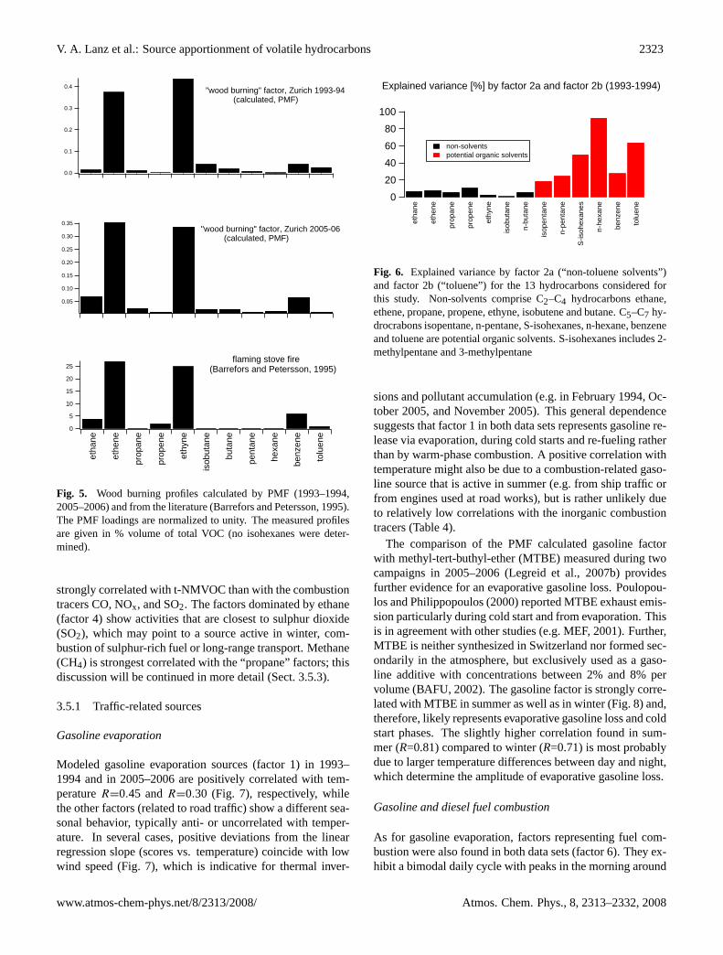
The ethane (2005–2006) and propane (1993–1994 and 2005–2006) dominated factors generally exhibit a diurnal patterndifferent from other hydrocarbon sources, i.e. a bimodaldaily cycle with maxima in the morning and late eveningas found for fuel combustion (Sect. 3.5.1). In contrast, thediurnal patterns of the propane and ethane dominated fac-tors are generally characterized by an early morning max-

imum and a mid-afternoon minimum, which was observedfor measured methane as well. This behavior is shown for the1993–1994 and 2005–2006 data in Fig. 11. Generally sucha behavior is interpreted as accumulation during the nightunder a shallow inversion layer followed by reducing con-centrations as the boundary layer expands during the morn-ing and early afternoon (e.g. Derwent et al., 2000). Con-centrations are therefore highest when the boundary layeris smallest and lowest when the boundary layer is highest.This implies that these emission rates must be reasonablyconstant between day and night. The medians between mid-night and 04:00 a.m. (small traffic contribution) increase lin-early for the propane and ethane factor, but also for mea-sured methane in 2005–2006 (Fig. 11): an emission ratiofor methane:“ethane”:“propane” of about 180:3:1 can be de-duced. Natural gas leakage is an obvious candidate for themain urban source of these hydrocarbons, especially as acompositional ratio (per volume) of 190(±129):3.7(±0.8):1(methane:ethane:propane) can be deduced for transportednatural gas in Zurich (Erdgas Ostschweiz AG, Zurich,2005/2006, unpublished data). These large uncertaintiesmainly reflect the variable gas mix, and might explain whygas leakage is represented by two factors rather than by onefactor. Natural gas consumption in [GWh] increased by 50%from 1992 to 2005 in Switzerland; it is typically more thanfour times higher in winter than in summer, which wouldexplain its correlation with SO2. For the early data (1993–1994), the presence of ethyne (Fig. 6) and a weak bimodaldaily cycle (Fig. 11) point to the possibility that the ethane




20

15

10

5

0

12108642

3.0

2.8

2.6

2.4

2.2

2.0

1.8

1.612108642

10

8

6

4

2

"ethane" 1993-94 (factor 4) 2005-06 (2.5 • factor 4)

temperature, °C 1993-94 2005-06

Month of the year

ppb

wind speed, m/s 1993-94 2005-06

"wood burning" 1993-94 (factor 5) 2005-06 (2.5 • factor 5)

Fig. 10. Factors representing wood burning (brown) and the“ethane” factors (orange), measured temperature (red) and windspeed (green) as monthly medians in 1993–1994 and 2005–2006(dashed).

Fig. 10. Factors representing wood burning (brown) and the“ethane” factors (orange), measured temperature (red) and windspeed (green) as monthly medians in 1993–1994 and 2005–2006(dashed).

factor was then also influenced by incomplete combustion,possibly from residential (gas or oil) heating due to its yearlytrend similar to that of wood burning (Fig. 10). It finally hasto be noticed that factors 3 and 4 in both data sets predomi-nantly explain the variability (>60%) of ethane and propane,respectively. The normalized loadings of other hydrocarbonsthan ethane and propane (e.g. butane in the “propane” factorfrom 2005–2006) do not represent their explained variability,but are, in other words, partially floating species within thementioned factors.

Due to their relatively long atmospheric lifetimes (days toweeks), propane and ethane (also from other sources thangas leakage) tend to accumulate in the air. Therefore, wecan not completely rule out that the factors “ethane” and“propane” may also represent aged VOC emissions as sus-pected by Buzcu and Fraser (2006). However, given theseasonal and diurnal patterns of those factors (Fig. 10 andFig. 11) the contribution of processed VOC source emis-sions can not be of a major importance. For aged and sec-ondary organic aerosols (SOA) with similar lifetimes (daysto weeks as the considered hydrocarbons) Lanz et al. (2007and 2008) have calculated increasing concentrations in theearly after-noon (due to elevated photochemical activity) andonly a slight enhancement of their mean concentrations inthe winter (5.3µg m−3) compared to summer (4.4µg m−3),as stronger accumulation and partitioning of volatile precur-sors outweigh less solar radiation in wintertime (Strader etal., 1999). Furthermore, ethane and propane concentrationsreported for European background air exhibit different levelsand time trends than the factors as calculated for the urbansite here (also see Sect. 4). Firstly, the ethane factors, as an

example, showed 3–8 times higher concentrations than re-ported for ethane in Finnish background air (Hakola et al.,2006). Note that ethane is decomposed faster at mid lati-tudes than in Polar air (due to the temperature dependence ofthe ethane-OH reaction rate constant and [OH] levels). Sec-ondly, we estimated that ethane and propane dominated fac-tors, most likely representing natural gas leakage, slightlydecreased by a factor of 1.3 from 1993–1994 to 2005–2006,whereas background ethane and propane showed increasingtrends between 1994 and 2003 (Hakola et al., 2006). Wetherefore conclude again that the hydrocarbon concentrationsmeasured at the urban background of Zurich-Kaserne can notbe significantly influenced by aged background air (also seeSects. 2.2.2 and 3.3.2).

3.5.4 Solvent usage

Acetates (belonging to the class of OVOCs) are commonlyused solvents in industry (Legreid et al., 2007b). Also Niedo-jadlo et al. (2007) measured elevated acetate concentrationsclose to industries in Wuppertal (Germany). A strong corre-lation was found between the sum of acetates (methyl-, ethyl,and butyl-) measured during two campaigns in 2005–2006and the calculated solvent factor for 2005–2006 (Fig. 12).Lower correlation of acetates in summertime (R=0.61) thanin wintertime (R=0.70) is possibly due to secondary forma-tion of acetates in the atmosphere, which is triggered by pho-tochemistry. Further note that factor 2 was derived for twoyears of data; it nevertheless seems representative of weeklyto daily variability of this hydrocarbon source.

3.6 Source contributions

Average source contributions as absolute concentrations[ppb] and relative [%] to the total mixing ratio of the 13 hy-drocarbons were calculated for both data sets and summa-rized in Table 5.

3.6.1 Representativeness of the 13 hydrocarbons

The concentrations of the 13 hydrocarbons considered in thisstudy accounted on average for 80–90% ppbC/ppbC of thesum of all 22 NMHC species measured at this site since 2005.Aromatic C8 hydrocarbons (m,p-xylene,o-xylene, and ethyl-benzene) represent a major fraction of that difference, ac-counting for more than 6% of the total concentration [ppb]of the 22 NMHCs. They were not measured continuouslyin 1993 and 1994. A PMF analysis of the extended dataset (2005–2006; comp. Sect. 3.3.1) revealed that those latteraromatics will be attributed to solvent use (60%), fuel com-bustion (30%), gasoline evaporation (5%), and wood burning(3%).

The 22 NMHCs plus the 22 oxidized VOCs compounds(∼20%; measured during four seasonal campaigns in 2005and 2006, Sect. 2.1.2) sum up to 78%-85% of the t-NMVOCconcentrations (in ppbC) determined by FID. For the earlier




0 3 6 9 12 16 20

02

46

8

factor 4 (’ethane’): 1993−94

Hour of the day

ppb

0 3 6 9 12 16 20

01

23

45

factor 3 (’propane’): 1993−94

Hour of the daypp

b0 3 6 9 12 16 20

1.7

1.8

1.9

2.0

2.1

2.2

2.3

2.4

methane (measured): 1993−94

Hour of the day

ppm

0 3 6 9 12 16 20

02

46

8

factor 4 (’ethane’): 2005−06

Hour of the day

ppb

0 3 6 9 12 16 20

01

23

45

factor 3 (’propane’): 2005−06

Hour of the day

ppb

0 3 6 9 12 16 20

1.7

1.8

1.9

2.0

2.1

2.2

2.3

2.4

methane (measured): 2005−06

Hour of the day

ppm

Fig. 11. Hourly boxplots of factors dominated by ethane (left) andpropane (middle), measured methane (right) for 1993–1994 (top)and 2005–2006 (bottom).

Fig. 11. Hourly boxplots of factors dominated by ethane (left) and propane (middle), measured methane (right) for 1993–1994 (top) and2005–2006 (bottom).

data (1993–1994), the 18 NMHCs (measured by GC-FID)accounted for 63% of t-NMVOC (FID) on average. In thelatter campaign, OVOCs were not determined directly, butvia the subtraction of non-oxidized NMHCs (retrieved byGC-FID and measurements of passive samplers) from thet-NMVOC signal we can say that about 20% or less VOCswere oxidized. Unlike the hydrocarbons used in this study,most OVOCs can be both directly released into the atmo-sphere or formed there secondarily. Furthermore they canbe of anthropogenic as well as biogenic origin (Legreid etal., 2007b). We therefore conclude that the 13 hydrocarbonsused in the present study are representative for primary andanthropogenic hydrocarbon emissions in Zurich.

3.7 Hydrocarbon emission trends (1993–1994 vs. 2005–2006)

For most hydrocarbon sources (road traffic, solvent use, andwood combustion) decreasing contributions by a factor of2–3 between 1993–1994 and 2005–2006 were modeled (Ta-ble 5 and Fig. 13). This trend is also reflected by the de-cline of t-NMVOC measurements (Fig. 1) and vice versa.However, for ethane and propane sources (mainly natural gasleakage), no such strong negative trend was found. In con-trast, propane and ethane sources only decreased by a fac-tor of 1.3 (but its consumption increased about 1.5 times).In Switzerland, steering taxes of about 2 Euro per kg VOCwere enforced in 1998. They are based on a black listof about 70 VOC species (e.g. toluene) or VOC classes(e.g. aromatic mixtures). Unlike most VOCs used in or assolvents, propane and ethane are not part of the black list(VOCV, 1997). The relatively constant ethane and propane



Table 5. Summary of hydrocarbon (sum of 13 C2 through C7 species) source apportionments for both periods 1993–1994 and 2005–2006and all factors. Factor grouping to classes of hydrocarbon sources.

mean rel. contr. median contr. 1. quart. 3. quart. mean conc.[%] [%] [%] [%] [ppb]

PMF factors2005–2006factor 1 “gasoline evaporation” 13 13 8 18 1.7factor 2 “solvents” 20 20 13 27 2.7factor 3 “propane” 14 14 10 18 1.9factor 4 “ethane” 21 19 13 27 2.7factor 5 “wood burning” 16 15 10 20 2.1factor 6 “fuel combustion” 13 13 9 17 1.7total explained mass conc. 97%average total conc. 13.2 ppb1993–1994factor 1 “gasoline evaporation” 15 13 9 18 3.7factor 2a “non-toluene solvents” 10 9 8 11 2.4factor 2b “toluene” 8 7 5 10 2.0factor 3 “propane” 8 7 4 10 1.9factor 4 “ethane” 17 15 9 23 4.1factor 5 “wood burning” 17 17 12 22 4.2factor 6 “fuel combustion” 11 11 8 13 2.6factor 7 “earlier traffic source” 15 14 9 19 3.6total explained mass conc. 99%average total conc. 24.8 ppb

Source groups2005–2006factor 1, 6 road traffic 26 26 20 33 3.5factor 2 solvent use 20 20 13 27 2.7factor 5 wood burning 16 15 10 20 2.1factor 3, 4 gas leakage 35 33 25 43 4.61993–1994factor 1, 6, 7 road traffic 40 38 26 50 9.9factor 2a, 2b solvent use 18 17 13 21 4.4factor 5 wood burning 17 17 12 22 4.2factor 3, 4 gas leakage 24 22 13 33 6.0

levels from gas leakage are in agreement with relatively con-stant methane concentrations measured in 1993–1994 and2005–2006: ethane (1%–6%) and propane (∼1%) are minorcomponents of natural gas, which predominantly consists ofmethane (>90%). On the other hand, methane has a life-time of years and is emitted by other sources as well (e.g. in-complete combustion of fossil and non-fossil materials) andtherefore no perfect correlation can be expected.

3.7.1 Traffic-related sources and solvent use

The EMEP (Cooperative Programme for Monitoring andEvaluation of the Long-range Transmission of Air Pollutantsin Europe) emission inventory for Switzerland (1993 versus2004) suggests that the most dominant VOC sources, i.e. sol-vent use (115×106 kg or 55% of t-NMVOC in 1993) and

road transport (63×106 kg or 30% of t-NMVOC in 1993) de-creased by a factor of two and three, respectively (Vestrenget al., 2006). Roughly the same relative decrease for roadtraffic and solvent use can be deduced from the data pre-sented in Table 5 and Fig. 13. However, we estimate thattraffic is still an important VOC emission source accountingon average for 40% ppb/ppb (1993–1994) and 26% ppb/ppb(2005–2006) of the total mixing ratio of the 13 hydrocar-bons (or 43%µg m−3/µg m−3 and 27%µg m−3/µg m−3,respectively). In contrast, solvent usage contributed on av-erage only to about 20% ppb/ppb (and about 5%–10% moreif based onµg m−3/µg m−3) of the ambient levels of the 13hydrocarbons measured at Zurich-Kaserne. For the 1993–1994 data Staehelin et al. (2001) (details in Sect. 3.4.2) havealso found that road traffic contributes at least twice as muchto ambient hydrocarbon concentrations than solvents, which




Winter: 19 December 2005 - 1 February 2006 (n=594)

Summer: 1 July - 1 August 2005 (n=340)

2.0

1.5

1.0

0.5

27.12.2005 06.01.2006 16.01.2006 26.01.2006

6

4

2

0

sum of acetates (measured) factor 2 ("solvents")

R=0.70ppb ppb

1.2

0.8

0.4

11.07.2005 21.07.2005 31.07.2005

16

12

8

4

0

R = 0.61

ppbppb

Fig. 12. Scores of factor 2 (“solvent use”) and the sum of mea-sured organic acetates (green) for the summer 2005 (bottom) andwinter 2005/2006 (top). The sum of measured acetates comprisesmethylacetate, ethylacetate and butylacetate, measured during twocampaigns.

Fig. 12. Scores of factor 2 (“solvent use”) and the sum of mea-sured organic acetates (green) for the summer 2005 (bottom) andwinter 2005/2006 (top). The sum of measured acetates comprisesmethylacetate, ethylacetate and butylacetate, measured during twocampaigns.

is in line with our findings. From the EMEP emission inven-tory for Switzerland, the emission ratio of “road transport” to“solvent and other production use” approximates 1:1.8 kg/kg(data for the year 1993; Vestreng et al., 2006), whereas aratio of 2.2:1 ppb/ppb (or 1.7:1µg m−3/µg m−3) road traf-fic:solvent use can be derived from our calculations. Thefact that we did not include OVOC species can not accountfor this discrepancy, as OVOCs measured at Zurich-Kaserneamounted to. 20% ppbC/ppbC of t-NMVOCs. In addi-tion, a considerable fraction of ambient OVOCs quantified atZurich-Kaserne is biogenic or secondarily formed (Legreidet al., 2007b). However, the comparability of the two ap-proaches (emission inventory and receptor modeling) is lim-ited by other instances, which are discussed in Sect. 4.

Vehicle emissions were limited by law since the 1980s,propagating the use of catalyst converters. Generally, road-traffic sources diminished by a factor of nearly three be-tween 1993–1994 and 2005–2006 (Fig. 13). However, thefuel combustion factor (strongly influenced by diesel contri-butions) only decreased by a factor of 1.5. A full catalystpenetration for gasoline driven passenger cars has been en-forced. For the diesel fleet, however, this is different and thismight also explain the rather similar hydrocarbon fingerprintfor the fuel combustion factor found in 1993–1994 and in2005–2006 (Sect. 3.4). On the other hand, gasoline evapo-ration showed a decrease by a factor of 2.2. We can explainthis reduction of evaporative loss by the introduction of va-por recovery systems at Swiss gasoline stations during thelate 1990s.


20

15

10

5

01993-94 2005-06

natural gas road traffic solvent usage wood burning other sources

35%

18%

17%20%

16%

26%

ppb

6.0 ppb

9.9 ppb

4.5 ppb

4.2 ppb2.1 ppb

2.7 ppb

3.5 ppb

4.6 ppb

40%

24%

0.8x

0.4x

0.6x

0.5x

Fig. 13. Bar chart showing the relative [%] and absolute [ppb]source contributions for 13 hydrocarbons at Zurich-Kaserne (urbanbackground) for 1993–1994 and 2005–2006. Factors were groupedto source classes as listed in Table 5.

Fig. 13. Bar chart showing the relative [%] and absolute [ppb]source contributions for 13 hydrocarbons at Zurich-Kaserne (urbanbackground) for 1993–1994 and 2005–2006. Factors were groupedto source classes as listed in Table 5.

4 Conclusions

Underlying factors of two year-long data sets of 13 volatilehydrocarbons (C2–C7) were described by bilinear receptormodeling (PMF) and related to different source categories:gasoline and diesel fuel combustion, gasoline evaporation,solvent use, wood burning, and natural gas leakage. Withdifferent numbers of factors for the 1993–1994 (p=8) and2005–2006 (p=6) data we accounted for the different emis-sion situations prevailing in the two periods and thereby com-parability between the factor analytical results was achieved.In contrast to a traditional CMB based analysis, no sourceprofiles are imposed within the PMF approach to calculatethe source activities, and the profiles are estimated as well.Consequently, we allowed for any changes in the nature andnumber of VOC source profiles, which obviously representsan advantage of an analysis based on PMF. We furthermorehave provided evidence that yearly PMF factors are repre-sentative for short-term source variability (days to weeks) bycomparing factor scores to tracer OVOCs (methyl-tert-butyl-ether and acetates). To our knowledge it was not reported be-fore that the number of dominating emission sources changedover time, which is however plausible due to large emissionreductions. The disappearance of a factor representing ex-haust emissions of gasoline road traffic is in accordance withthe measurements in a nearby road tunnel (Gubrist tunnel)showing the successful introduction of catalytic convertersin the Swiss road traffic fleet.

The emissions of the 13 hydrocarbons from combustionsources (road traffic and wood burning) as well as solventuse decreased by a factor of two to three, while factors thatmostly represent natural gas leakage remained at relativelyconstant levels between 1993–1994 and 2005–2006. Thisgeneral result is in line with conclusions drawn by Dollard etal. (2007) for similar sites (urban background) in the United



Kingdom: while ethane concentrations pointing to naturalgas leakage remained at constant levels between 1993 and2004, a yearly decrease by−15% and−28% could be ob-served for vehicle exhaust tracing ethene and propene, re-spectively. A decrease of road traffic emissions by a factorof 2.8 during 12 years as estimated in this study is thereforealso in line with findings from other European urban back-ground locations. Note that the loss of natural gas relative toits transported amount also decreased by more than a factorof two as its consumption increased by 50% between 1992and 2005.

In agreement with Niedojadlo et al. (2007; CMB anal-ysis of ambient hydrocarbons in a German city), we alsofound that there is inconsistency between national emissioninventories (such as the EMEP inventory; Vestreng et al.,2006) and source apportionment based on multivariate re-ceptor modeling: according to emission inventories, solventuse is a more important VOC source than road traffic, but theopposite is concluded from the receptor models. We hypoth-esize that solvent VOCs used for industrial purposes havebeen being substituted by less toxic and oxidized VOCs forthe last 30 years. In fact, oxidized compounds make up morethan 80% of Switzerland’s imported solvent VOCs nowadays(R. Weber, FOEN, personal comm.). However, the fact that acertain amount of VOCs used in solvents are oxidized species(which are not covered in this study) is not sufficient to ex-plain the disagreement between bottom-up (i.e. emission in-ventories) and top-down approaches (i.e. modeling sourcesfrom field measurements); the OVOCs’ apportioned share inambient t-NMVOC is too low (≤20% ppbC/ppbC) and, ad-ditionally, a major fraction of these OVOCs in turn could berelated to biogenic release, secondary formation and com-bustion sources (Legreid et al., 2007b). More importantly,this comparison is inherently difficult as emission inventoriesprovide average data valid on a national scale, while the spa-tial representativeness of data from a single measurement siteis typically much smaller. Many city centers in Europe andNorth-America today predominantly harbor service sectors,while manufacturing industries moved to suburban or remoteplaces, which means that Zurich might be biased towardstraffic emissions. Correspondingly, we can expect that VOCsused as solvents for industrial purposes are more likely to belost (due to degradation, interception, etc.) during transportfrom source to the urban receptor site, explaining the moreprominent importance of solvent sources reported in nationalemission inventories. A minor issue is the reduced transmis-sion efficiencies for long-chained and oxidized hydrocarbonsthat may adsorb on the surface of the inlet tubes to a greaterextend. It should further be noted that source categories inemission inventories may not fully match the source groupsrepresented by PMF factors in all cases, adding uncertaintyto this comparison as well. Future applications of the pre-sented approach to data from more industrialized regions areexpected to clarify the differences between the results ob-tained by the two methodologies.

Acknowledgements.The OVOC measurements were supportedby the Swiss Federal Office for the Environment (FOEN). Wethank U. Lohmann (ETH), A. Prevot (PSI), H. Hellen (FMI) andR. Weber (FOEN) for their critical comments and suggestionswhich improved this paper. The earlier hydrocarbon data wereprovided by AWEL (Kanton Zurich’s Department for Waste, Water,Energy, and Air). The current VOC data are measured withinthe National Air Pollution Monitoring Network (NABEL). Manythanks to Bo Larsen, Stephane Sauvage, and an anonymous referee.

Edited by: J. Abbatt

References

Anttila, P., Paatero, P., Tapper, U., and Jarvinen, O.: Source iden-tification of bulk wet deposition in Finland by positive matrixfactorization, Atmos. Environ., 29, 1705–1718, 1995.

Atkinson, R. and Arey, J.: Atmospheric degradation of volatile or-ganic compounds, Chem. Rev., 103, 4605–4638, 2003.

BAFU: Luftschadstoff-Emissionen des Stassenverkehrs 1950–2020. Nachtrag. Schriftenreihe UMWELT Nr. 225, Swiss Fed-eral Office for the Environment FOEN, Bern, 2000.

BAFU: Abschatzung der Altlastenrelevanz von Methyl-tert-butylether (MTBE). Swiss Federal Office for the Environ-ment FOEN, Bern, available at:http://www.bafu.admin.ch/php/modules/shop/files/pdf/phpyeb9SE.pdf, 2002.

BAFU: Anthropogene VOC-Emissionen Schweiz 1998, 2001 und2004, Swiss Federal Office for the Environment FOEN, Bern,available at:http://www.bafu.admin.ch/voc/03756/03758/index.html?lang=de, 2007.

Barrefors, G. and Petersson, G.: Volatile hydrocarbons from do-mestic wood burning, Chemosphere, 30, 1551–1556, 1995.

Bartenbach, S., Williams, J., Plass-Duelmer, C., Berresheim, H.,and Lelieveld, J.: In-situ measurement of reactive hydrocarbonsat Hohenpeissenberg with comprehensive two-dimensional gaschromatography (GCxGC-FID): use in estimating HO and NO3,Atmos. Chem. Phys., 7, 1-14, 2007,http://www.atmos-chem-phys.net/7/1/2007/.

Blifford, I. H. and Meeker, G. O.: A factor analysis model of largescale pollution, Atmos. Environ., 1, 147–157, 1967.

Borbon, A., Coddeville, P., Locoge, N., and Galloo, J.-C.: Char-acterising sources and sinks of rural VOC in eastern France,Chemosphere, 57, 931–942, 2004.

Buset, K. C., Evans, G. J., Leaitch, W. R., Brook, J. R., Toom-Sauntry, D.: Use of advanced receptor modelling for analysis ofan intensive 5-week aerosol sampling campaign, Atmos. Envi-ron., 40, Suppl 2, 482–499, 2006.

Buzcu, B. and Frazier, M. P.: Source identification and apportion-ment of volatile organic compounds in Houston, TX, Atmos. En-viron., 40, 2385–2400, 2006.

Christensen, W. F., Schauer, J. J., and Lingwall, J. F.: Iterated con-firmatory factor analysis for pollution source apportionment, En-vironmetrics, 17, 663–681, 2006.

Colberg, C. A., Tona, B., Stahel, W. A., Meier, M., and Staehelin,J.: Comparison of a road traffic emission model (HBEFA) withemissions derived from measurements in the Gubrist road tunnel,Switzerland, Atmos. Environ., 39, 4703–4714, 2005.

Derwent, R. G., Davies, T. J., Delaney, M., Dollard, G. J., Field,R. A., Dumitrean, P., Nason, P. D., Jones, B. M. R., and Pepler,


http://www.bafu.admin.ch/php/ modules/shop/files/pdf/phpyeb9SE.pdf

http://www.bafu.admin.ch/php/ modules/shop/files/pdf/phpyeb9SE.pdf

http://www.bafu.admin.ch/voc/03756/03758/index.html?lang=de

http://www.bafu.admin.ch/voc/03756/03758/index.html?lang=de

http://www.atmos-chem-phys.net/7/1/2007/


S. A.: Analysis and interpretation of the continuous hourly mon-itoring data for 26 C2–C8 hydrocarbons at 12 United Kingdomsites during 1996, Atmos. Environ., 34, 297–312, 2000.

Dollard, G. J., Dumitrean, P., Telling, S., Dixon, J., and Derwent,R. G: Observed trends in ambient concentrations of C2–C8 hy-drocarbons in the United Kingdom over the period from 1993 to2004, Atmos. Environ., 41, 2559–2569, 2007.

Eggertsen, F. T. and Nelsen, F. M.: Gas chromatographic analysisof engine exhaust and atmopshere. Determination of C2–C5 hy-drocarbons, Anal. Chem., 30, 1040–1043, 1958.

Empa: Technischer Bericht zum Nationalen Beobachtungsnetz furLuftfremdstoffe (NABEL), available at:http://www.empa.ch/nabel, Dubendorf, Switzerland, 2006.

Forster, P., Ramaswamy, V., Artaxo, P., Berntsen, T. , Betts, R.,Fahey, D.W., Haywood, J., Lean, J., Lowe, D. C., Myhre, G.,Nganga, J., Prinn, R., Raga, G., Schulz, M., and Van Dorland, R.:Changes in atmospheric constituents and in radiative forcing, in:Climate Change 2007: The Physical Science Basis. Contributionof Working Group I to the Fourth Assessment Report of the In-tergovernmental Panel on Climate Change, edited by: Solomon,S., Qin, D., Manning, M., Chen, Z., Marquis, M., Averyt, K.B., Tignor, M., and Miller, H. L., Cambridge University Press,Cambridge, United Kingdom and New York, NY, USA, 2007.

Fujita, E. M., Campbell, D. E., Zielinska, B., Sagebiel, J. C.,Bowen, J. L., Goliff, W. S., Stockwell, W. S., and Lawson, D.R.: Diurnal and weekday variations in the source contributionsof ozone precursors in California’s South Coast Air Basin, J. AirWaste Manage., 53, 844–863, 2003.

Fuzzi, S., Andreae, M. O., Huebert, B. J., Kulmala, M., Bond,T. C., Boy, M., Doherty, S. J., Guenther, A., Kanakidou, M.,Kawamura, K., Kerminen, V.-M., Lohmann, U., Russell, L. M.,and Poschl, U.: Critical assessment of the current state of scien-tific knowledge, terminology, and research needs concerning therole of organic aerosols in the atmosphere, climate, and globalchange, Atmos. Chem. Phys., 6, 2017–2038, 2006,http://www.atmos-chem-phys.net/6/2017/2006/.

Hakola, H., Hellen, H., and Laurila, T.: Ten years of light hydrocar-bons (C2–C6) concentration measurements in background air inFinland, Atmos. Environ., 40, 3621–3630, 2006.

HBEFA: Handbuch fur Emissionsfaktoren des Strassenverkehrs(handbook of emission factors for road traffic), Umweltbun-desamt Berlin, Bundesamt fur Umwelt, Wald und LandschaftBern, Infras AG, Bern (published on CD-ROM, also availableat: www.hbefa.net), 2004.

Hellen, H., Hakola, H., Pirjola, L., Laurila, T., and Pystynen, K.-H.:Ambient air concentrations, source profiles, and source appor-tionment of 71 Different C2–C10 volatile organic compounds inurban and residential areas of Finland, Environ. Sci. Technol.,40, 103–108, 2006.

Henry, R. C., Lewis, C. W., Hopke, P. K., and Williamson, H. J.:Review of receptor model fundamentals, Atmos. Environ., 18,1507–1515, 1984.

Henry, R. C.: Multivariate receptor modelling by N-dimensionaledge detection, Chemometr. Intell. Lab., 65, 179–189, 2003.

Hopke, P. K.: Target transformation factor analysis as an aerosolmass apportionment method: A review and sensitivity analysis,Atmos. Environ., 22, 1777-1792, 1988.

Hopke, P. K.: Recent developments in receptor modeling,Chemometr. Intell. Lab., 17, 255–265, 2003.

Jorquera, H. and Rappengluck, B.: Receptor modeling of ambientVOC at Santiago, Chile, Atmos. Environ., 38, 4243–4263, 2004.

Junninen, H., Niska, H., Tuppurainen, K., Ruuskanen, J., andKolehmainen, M.: Methods for imputation of missing values inair quality data sets, Atmos. Environ., 38, 2895–2907, 2004.

Kunert, U. and Kuhfeld, H.: The diverse structures of passenger cartaxation in Europe and the EU Commissions proposal for reform,Transp. Policy, 14, 306–316, 2007.

Lanz, V. A., Alfarra, M. R., Baltensperger, U., Buchmann, B.,Hueglin, C., and Prevot, A. S. H.: Source apportionment of sub-micron organic aerosols at an urban site by factor analytical mod-elling of aerosol mass spectra, Atmos. Chem. Phys., 7, 1503-1522, 2007,http://www.atmos-chem-phys.net/7/1503/2007/.

Lanz, V. A., Alfarra, M. R., Baltensperger, U., Buchmann, B.,Hueglin, C., Szidat, S., Wehrli, M. N., Wacker, L., Weimer, S.,Caseiro, A., Puxbaum, H., and Prevot, A. S. H.: Source attribu-tion of submicron organic aerosols during wintertime inversionsby advanced factor analysis of aerosol mass spectra, Environ.Sci. Technol., 42, 214–220, 2008.

Latella, A., Stani, G., Cobelli, L., Duane, M., Junninen, H., As-torga, C., and Larsen, B. R.: Semicontinuous GC analysis andreceptor modelling for source apportionment of ozone precursorhydrocarbons in Bresso, Milan, 2003, J. Chrom. A, 39, 29–39,2005.

Lee, E., Chan, C., and Paatero, P.: Application of positive matrixfactorization in source apportionment of particulate pollutants inHong Kong, Atmos. Environ., 33, 3201–3212, 1999.

Legreid, G., Reimann, S., Steinbacher, M., Staehelin, J., Young, D.,and Stemmler, K.: Measurements of OVOCs and NMHCs in aSwiss highway tunnel for estimation of road transport emissions,Environ. Sci. Technol., 41, 7060–7066, 2007a.

Legreid, G., Balzani Loov, J., Staehelin, J., Hueglin, C., Hill, M.,Buchmann, B., Prevot, A. S. H., and Reimann, S.: Oxygenatedvolatile organic compounds (OVOCs) at an urban backgroundsite in Zurich (Europe): Seasonal variation and source allocation,Atmos. Environ., 41, 8409–8423, 2007b.

Li, Z., Hopke, P. K., Husain, L., Qureshi, S., Dutkiewicz, V. A.,Schwab, J. J., Drewnick, F., and Demerjian, K. L.: Sources offine particle composition in New York City, Atmos. Environ., 38,6521–6529, 2004.

Matson, P., Lohse, K. A., and Hall, S. J.: The globalization of nitro-gen deposition: Consequences for terrestrial ecosystems, Ambio,31, 113–119, 2002.

McKendry, I. G., Steyn, D. G., Lundgren, J., Hoff, R. M., Strapp,W., Anlauf, K., Froude, F., Martin, J. B., Banta, R. M., andOlivier, L. D.: Elevated ozone layers and vertical down-mixingover the Lower Fraser Valley, BC, Atmos. Environ., 31, 2135-2146, 1997.

MEF: MEF, Risk assessment of methyl tertiary-butyl ether(MTBE), EINECS No 216-653-1, carried out in the frameworkof European Council Regulation (EEC) 793/93 on the evaluationand control of the risks of existing substances, Ministry of theEnvironment Finland, Helsinki, Final Draft 06/2001, 328, 2001.

Miller, S. L., Anderson, M. J., Daly, E. P., and Milford, J. B.: Sourceapportionment of exposures to volatile organic compounds. I.Evaluation of receptor models using simulated exposure data, At-mos. Environ., 36, 3629–3641, 2002.

Nel, A.: Air pollution-related illness: effects of particles, Science,


http://www.empa.ch/nabel

http://www.empa.ch/nabel


www.hbefa.net



308, 804–806, 2005.Niedojadło, A., Becker, K. H., Kurtenbach, R., and Wiesen, P.: The

contribution of traffic and solvent use to total NMVOC emissionin a German city derived from measurements and CMB mod-elling, Atmos. Environ., 41, 7108–7126, 2007.

Olson, M.: Wheat straw and peat fuel pellets - organic compoundsfrom combustion, Biomass Bioenerg., 30, 555–564, 2006.

Paatero, P. and Tapper, U.: Positive matrix factorization: a non-negative factor model with optimal utilization of error estimatesof data values, Environmetrics, 5, 111–126, 1994.

Paatero, P.: Least squares formulation of robust non-negative factoranalysis, Chemometr. Intell. Lab., 37, 23–35, 1997.

Paatero, P.: User’s guide for positive matrix factorization programsPMF2 and PMF3, part 1: tutorial, University of Helsinki, Fin-land, 2007.

Paatero, P., Hopke, P. K., Begum, B. A., and Biswas, S. K.: Agraphical diagnostic method for assessing the rotation in factoranalytical models of atmospheric pollution, Atmos. Environ., 39,193–201, 2005.

Poulopoulos, S. and Philippopoulos, C.: Influence of MTBE addi-tion into gasoline on automotive exhaust emissions, Atmos. En-viron., 34, 4781–4786, 2000.

Primerano, P., Marino, G., Di Pasquale, S., Mavilia, L., andCorigliano, F.: Possible alteration of monuments caused by parti-cles emitted into the atmosphere carrying strong primary acidity,Atmos. Environ., 34, 3889–3896, 2000.

Ruffieux, D., Nash, J., Jeannet, P., and Agnew, J. L.: The COST720 temperature, humidity, and cloud profiling campaign: TUC,Meteorol. Z., 15, 5-10, 2006.

Schauer, J. J., Rogge, W. F., Hildemann, L. M., Mazurek, M. A.,and Cass, G. R.: Source apportionment of airborne particulatematter using organic compounds as tracers, Atmos. Environ., 30,3837–3855, 1996.

Seinfeld, J. H. and Pandis, S. N.: Atmospheric chemistry andphysics, John Wiley and Sons, Inc., New York, 1998.

Staehelin, J., Keller, C., Stahel, W., Schlapfer, K., and Wunderli, S.:Emission factors from road traffic from a tunnel study (Gubristtunnel, Switzerland), Part III: Results of organic compounds,SO2, and speciation of oranic exhaust emission, Atmos. Envi-ron., 32, 999–1009, 1998.

Staehelin, J., Locher, R., Monkeberg, S., and Stahel, W. A.: Con-tribution of road traffic emissions to ambient air concentrationsof hydrocarbons: the interpretation of monitoring measurementsin Switzerland by Principal Component Analysis and road tunnelmeasurements, Int. J. Vehicle Des., 27, 161–172, 2001.

Strader, R., Lurmann, F., and Pandis, S. N.: Evaluation of secondaryorganic aerosol formation in winter, Atmos. Environ., 33, 4849–4863, 1999.

Theloke, J. and Friedrich, R.: Compilation of a database on thecomposition of anthropogenic VOC emissions for atmosphericmodeling in Europe, Atmos. Environ., 41, 4148–4160, 2007.

Vestreng, V., Rigler, E., Adams, M., Kindbom, K., Pacyna, J. M.,Denier van der Gon, H., Reis, S., and Travnikov, O.: Inventoryreview 2006, Emission data reported to LRTAP and NEC Direc-tive, Stage 1, 2 and 3 review and Evaluation of inventories ofHM and POPs. EMEP/MSC-W Technical Report 1/2006 ISSN1504-6179, available at:http://www.emep.int, 2006.

VOCV: http://www.admin.ch/ch/d/sr/c814018.html, 1997.Wahlin, P.: COPREM – A multivariate receptor model with a phys-

ical approach, Atmos. Environ., 37, 4861-4667, 2003.Watson, J. G.: Visibility: science and regulation, J. Waste Air Man-

age., 52, 628–713, 2002.WHO: Benzene (Environmental Health Criteria, No. 150), Geneva,

World Health Organization, 1993.Winchester, J. W. and Nifong, G. D.: Water pollution in Lake

Michigan by trace elements from pollution aerosol fallout, WaterAir Soil Poll., 1, 51–64, 1971.

Zhao, W., Hopke, P. K., and Karl, T.: Source Identification ofvolatile organic compounds in Houston, TX, Environ. Sci. Tech-nol., 38, 1338–1347, 2004.


http://www.emep.int

http://www.admin.ch/ch/d/sr/c814_018.html

Documents

Receptor modeling of C2–C7 hydrocarbon sources at an urban