The University of Southern Mississippi The University of Southern Mississippi

The Aquila Digital Community The Aquila Digital Community

Dissertations

Fall 2017

Radial Basis Function Differential Quadrature Method for the Radial Basis Function Differential Quadrature Method for the

Numerical Solution of Partial Differential Equations Numerical Solution of Partial Differential Equations

Daniel Watson University of Southern Mississippi

Follow this and additional works at: https://aquila.usm.edu/dissertations

Part of the Numerical Analysis and Computation Commons, and the Partial Differential Equations

Commons

Recommended Citation Recommended Citation Watson, Daniel, "Radial Basis Function Differential Quadrature Method for the Numerical Solution of Partial Differential Equations" (2017). Dissertations. 1468. https://aquila.usm.edu/dissertations/1468

This Dissertation is brought to you for free and open access by The Aquila Digital Community. It has been accepted for inclusion in Dissertations by an authorized administrator of The Aquila Digital Community. For more information, please contact Joshua.Cromwell@usm.edu.

The University of Southern MississippiThe Aquila Digital Community

Dissertations

Fall 2017

Radial Basis Function Differential QuadratureMethod for the Numerical Solution of PartialDifferential EquationsDaniel Watson

Follow this and additional works at: https://aquila.usm.edu/dissertations

Part of the Numerical Analysis and Computation Commons, and the Partial DifferentialEquations Commons

The University of Southern Mississippi

RADIAL BASIS FUNCTION DIFFERENTIAL QUADRATURE METHOD FOR THE

NUMERICAL SOLUTION OF PARTIAL DIFFERENTIAL EQUATIONS

by

Daniel Wade Watson

Abstract of a DissertationSubmitted to the Graduate School

and the Department of Mathematicsof The University of Southern Mississippiin Partial Fulfillment of the Requirements

for the Degree of Doctor of Philosophy

December 2017

RADIAL BASIS FUNCTION DIFFERENTIAL QUADRATURE METHOD FOR THE

NUMERICAL SOLUTION OF PARTIAL DIFFERENTIAL EQUATIONS

by

Daniel Wade Watson

A DissertationSubmitted to the Graduate School

and the Department of Mathematicsat The University of Southern Mississippiin Partial Fulfillment of the Requirements

for the Degree of Doctor of Philosophy

Approved:

Dr. Ching-Shyang Chen, Committee ChairProfessor, Mathematics

Dr. Haiyan Tian, Committee MemberProfessor, Mathematics

Dr. Zhifu Xie, Committee MemberProfessor, Mathematics

Dr. Huiqing Zhu, Committee MemberAssociate Professor, Mathematics

Dr. Karen S. CoatsDean of the Graduate School

December 2017

COPYRIGHT BY

DANIEL WADE WATSON

2017

ABSTRACT

RADIAL BASIS FUNCTION DIFFERENTIAL QUADRATURE METHOD FOR THE

NUMERICAL SOLUTION OF PARTIAL DIFFERENTIAL EQUATIONS

by Daniel Wade Watson

December 2017

In the numerical solution of partial differential equations (PDEs), there is a need for

solving large scale problems. The Radial Basis Function Differential Quadrature (RBF-

DQ) method and local RBF-DQ method are applied for the solutions of boundary value

problems in annular domains governed by the Poisson equation, inhomogeneous biharmonic

equation, and the inhomogeneous Cauchy-Navier equations of elasticity. By choosing the

collocation points properly, linear systems can be obtained so that the coefficient matrices

have block circulant structures. The resulting systems can be efficiently solved using matrix

decomposition algorithms (MDAs) and fast Fourier transforms (FFTs). For the local RBF-

DQ method, the MDAs used are modified to account for the sparsity of the arrays involved in

the discretization. An adjusted Fasshauer estimate is used to obtain a good shape parameter

value in the applied radial basis functions (RBFs) for the global RBF-DQ method while

the leave-one-out cross validation (LOOCV) algorithm is employed for the local RBF-DQ

method using a sample of local influence domains. A modification of the kdtree algorithm

is used to select the nearest centers for each local domain. In several numerical experiments,

it is shown that the proposed algorithms are capable of solving large scale problems while

maintaining high accuracy.

iii

ACKNOWLEDGMENTS

I would like to thank my advisor, Dr. C.S. Chen. He is an amazing mathematician who

makes the most difficult concepts appear simple. His passion of scientific computing and

problem solving has inspired me beyond measure. Without his continuous support, this

work would not have come to fruition.

I would also like to extend my sincere thanks to Dr. Karageorghis for sharing his expert

knowledge in the field. Though we have never officially met, our email correspondence has

been very valuable. I am also deeply grateful to my committee members Drs. Tian, Zhu,

and Xie for their continuous support, encouragement, and useful feedback in this work. I

am very fortunate to have support of my committee members.

I would like to express special thanks to my family. Without the unwavering support, en-

couragement, and sacrifice of my beautiful wife, Melinda, this would not have been possible.

Thank you to my wonderful children Linda Rose, Isaac, and Eli, for your understanding and

encouragement. I hope this shows you that you can do anything that you put your mind to.

Finally, my thanks goes to all of my friends at USM, my research group members Thir

R Dangal, Lei-Hsin Kuo, Balaram K Ghimire, and Anup R Lamichhane who were always

ready to help me out at any time. I especially thank Shannon Ryle. We have walked through

this journey together and I would not have made it without you my friend.

iv

TABLE OF CONTENTS

ABSTRACT . . . . . . . . . . . . . . . . . . . . . . . . . . . . . . . . . . iii

ACKNOWLEDGMENTS . . . . . . . . . . . . . . . . . . . . . . . . . . . . . i

LIST OF ILLUSTRATIONS . . . . . . . . . . . . . . . . . . . . . . . . . . iv

LIST OF TABLES . . . . . . . . . . . . . . . . . . . . . . . . . . . . . . . v

LIST OF ABBREVIATIONS . . . . . . . . . . . . . . . . . . . . . . . . . vii

NOTATION AND GLOSSARY . . . . . . . . . . . . . . . . . . . . . . . . viii

1 INTRODUCTION . . . . . . . . . . . . . . . . . . . . . . . . . . . . . . 11.1 Background 11.2 Literature Review 21.3 Synopsis 4

2 STATE-OF-THE-ART IN MESHLESS METHOD . . . . . . . . . . . . . 62.1 Radial Basis Function (RBF) Interpolation 62.2 The Collocation (Kansa) Method 72.3 The Method of Particular Solutions 82.4 Radial Basis Function Differential Quadrature Method 92.5 Local Radial Basis Function Differential Quadrature Method 112.6 Shape Parameter 13

3 MATRIX DECOMPOSITION ALGORITHM . . . . . . . . . . . . . . . 183.1 Matrix Decomposition 183.2 Circulant Matrices 223.3 Properties of Circulant Matrices 24

4 Global and Local RBF-DQ MDA . . . . . . . . . . . . . . . . . . . . . . 314.1 RBF-DQ MDA 314.2 Circulant Matrix Transform 454.3 Matrix Decomposition Algorithm for Cauchy-Navier 494.4 LRBF-DQ MDA 51

5 NUMERICAL RESULTS . . . . . . . . . . . . . . . . . . . . . . . . . . 575.1 Poisson Equation RBF-DQ 58

v

5.2 Biharmonic Equation RBF-DQ 635.3 Cauchy-Navier RBF-DQ 675.4 Poisson Equation LRBF-DQ 695.5 Biharmonic Equation LRBF-DQ 735.6 Cauchy-Navier LRBF-DQ 76

6 CONCLUSIONS AND FUTURE WORKS . . . . . . . . . . . . . . . . . 796.1 Conclusions 796.2 Future Works 81

INDEX . . . . . . . . . . . . . . . . . . . . . . . . . . . . . . . . . . . . 82

BIBLIOGRAPHY . . . . . . . . . . . . . . . . . . . . . . . . . . . . . . . 82

vi

LIST OF ILLUSTRATIONS

Figure

2.1 Choosing r0 in each local influence domain. . . . . . . . . . . . . . . . . . . . 17

3.1 Annulus Domain . . . . . . . . . . . . . . . . . . . . . . . . . . . . . . . . . 193.2 Discretization of the annuluar domain with (a) no rotation of the collocation

points and (b) with rotation of the collocation points. The crosses (+) denotethe collocation points. . . . . . . . . . . . . . . . . . . . . . . . . . . . . . . . 20

3.3 Distribution of collocation points on domain . . . . . . . . . . . . . . . . . . . 21

4.1 Distribution of collocation points in local domains. The four neighboring pointsfor the two centers (X) are highlighted. . . . . . . . . . . . . . . . . . . . . . . 53

5.1 Example 1: Profile of the Exact Solution. . . . . . . . . . . . . . . . . . . . . 585.2 Example 1: Profile of Relative Error. . . . . . . . . . . . . . . . . . . . . . . . 595.3 Example 1, Multiquadric (MQ): Maximum relative error vs. shape parameter,

M = 100,N = 100. . . . . . . . . . . . . . . . . . . . . . . . . . . . . . . . 605.4 Example 1, Inverse Multiquadric (IMQ): Maximum relative error vs. shape

parameter, M = 100,N = 100. . . . . . . . . . . . . . . . . . . . . . . . . . 605.5 Example 1, Gaussian (GA): Maximum relative error vs. shape parameter,

M = 100,N = 100. . . . . . . . . . . . . . . . . . . . . . . . . . . . . . . . 605.6 Example 1, Gaussian (GA): Maximum relative error versus shape parameter

with M = 100,N = 100. . . . . . . . . . . . . . . . . . . . . . . . . . . . . 615.7 Example 1, Poisson Dirichlet problem: Maximum relative error versus mx using

MQ. . . . . . . . . . . . . . . . . . . . . . . . . . . . . . . . . . . . . . . . . 615.8 Example 2: Profile of Relative Error. . . . . . . . . . . . . . . . . . . . . . . . 645.9 Example 2, First Biharmonic Problem: Maximum relative error versus shape

parameter with M = 100,N = 100 using MQ. . . . . . . . . . . . . . . . . 655.10 Example 3: Profile of the Exact Solutions, u1 and u2, respectively. . . . . . . . 685.11 Example 3, Cauchy Navier Dirichlet problem: Maximum relative error versus

shape parameter with M = 100,N = 100 using MQ RBF. . . . . . . . . . . 695.12 Example 4, Poisson Dirichlet problem: Maximum relative error versus dimen-

sionless shape parameter with M = N = 100 using MQ RBF. . . . . . . . . . . 715.13 Example 5: First Biharmonic problem: Error versus shape parameter for the

cases M = N = 80,200,n = 30 using MQ RBF. . . . . . . . . . . . . . . . . . 745.14 Example 6: Cauchy Navier problem. Maximum relative error versus shape

parameter for M = N = 100,n = 9 using MQ RBF. . . . . . . . . . . . . . . . 77

vii

LIST OF TABLES

Table

2.1 Globally supported RBFs. . . . . . . . . . . . . . . . . . . . . . . . . . . . . 7

5.1 Example 1, Optimal Shape Parameter c and Max Rel Error for MQ, IMQ, andGuassian RBFs . . . . . . . . . . . . . . . . . . . . . . . . . . . . . . . . . . 59

5.2 Example 1, Poisson Dirichlet Problem: Max Rel Error and shape parameterusing MQ. . . . . . . . . . . . . . . . . . . . . . . . . . . . . . . . . . . . . . 62

5.3 Example 1, Poisson Dirichlet problem: Max Rel Error and shape parameterusing MQ up to 1 million points . . . . . . . . . . . . . . . . . . . . . . . . . 62

5.4 Example 1, Poisson Dirichlet problem: Max Rel Error with c = 90 usingGaussian RBF. . . . . . . . . . . . . . . . . . . . . . . . . . . . . . . . . . . 62

5.5 Example 1, Poisson Neumann problem: Max Rel Error and shape parameterusing MQ RBF. . . . . . . . . . . . . . . . . . . . . . . . . . . . . . . . . . . 63

5.6 Example 1, Poisson Dirichlet problem: Comparison of Errors, E, and CPUtimes for full RBF-DQ and RBF-DQ MDA solutions for various M = N withinitial search interval [0,8]. . . . . . . . . . . . . . . . . . . . . . . . . . . . . 64

5.7 Example 2, First Biharmonic Problem: Max Rel Error and shape parameterusing MQ. . . . . . . . . . . . . . . . . . . . . . . . . . . . . . . . . . . . . . 65

5.8 Example 2, First Biharmonic problem: Max Rel Error with c = 60 usingGaussian RBF. . . . . . . . . . . . . . . . . . . . . . . . . . . . . . . . . . . 66

5.9 Example 2, Second Biharmonic problem: Max Rel Error and shape parameterusing MQ RBF. . . . . . . . . . . . . . . . . . . . . . . . . . . . . . . . . . . 66

5.10 Example 2, Second Biharmonic problem: Max Rel Error for c = 60 usingGaussian RBF. . . . . . . . . . . . . . . . . . . . . . . . . . . . . . . . . . . 66

5.11 Example 3, Cauchy Navier Dirichlet problem: Max Rel Error and shape param-eter using MQ RBF. . . . . . . . . . . . . . . . . . . . . . . . . . . . . . . . . 67

5.12 Example 3, Cauchy Navier Neumann/Dirichlet problem: Max Rel Error andshape parameter using MQ RBF. . . . . . . . . . . . . . . . . . . . . . . . . . 68

5.13 Example 3, Cauchy Navier Dirichlet problem: Max Rel Error with c = 90 usingGaussian RBF. . . . . . . . . . . . . . . . . . . . . . . . . . . . . . . . . . . 68

5.14 Example 3, Cauchy Navier Neumann/Dirichlet problem: Max Rel Error withc = 90 using Gaussian RBF. . . . . . . . . . . . . . . . . . . . . . . . . . . . 69

5.15 Example 4, Poisson Dirichlet problem: Max Rel Error and optimal shapeparameter with various search intervals of LOOCV for M = N = 200 usingMQ RBF. . . . . . . . . . . . . . . . . . . . . . . . . . . . . . . . . . . . . . 70

5.16 Example 4, Poisson Dirichlet problem: Max Rel Error and optimal shapeparameter via LOOCV for n = 9 using MQ RBF. . . . . . . . . . . . . . . . . 70

viii

5.17 Example 4, Poisson Neumann problem: Max Rel Error and optimal shapeparameter via LOOCV for n = 9 using MQ RBF. . . . . . . . . . . . . . . . . 71

5.18 Example 4, Poisson Dirichlet problem M = N = 200: Max Rel Error for dimen-sionless shape parameter using MQ RBF. . . . . . . . . . . . . . . . . . . . . 72

5.19 Example 4, Poisson Dirichlet problem: Max Rel Error with c=MN/1000 usingMQ RBF. . . . . . . . . . . . . . . . . . . . . . . . . . . . . . . . . . . . . . 72

5.20 Example 4, Poisson Neumann problem: Max Rel Error with c = MN/1000using MQ RBF. . . . . . . . . . . . . . . . . . . . . . . . . . . . . . . . . . . 73

5.21 Example 4, Poisson Dirichlet problem: Influence Domain for M=N=500 usingMQ RBF. . . . . . . . . . . . . . . . . . . . . . . . . . . . . . . . . . . . . . 73

5.22 Example 5, First Biharmonic problem: Max Rel Error and optimal shapeparameter via LOOCV for M = N = 80 using MQ RBF. . . . . . . . . . . . . 75

5.23 Example 5, Second Biharmonic problem: Max Rel Error and optimal shapeparameter via LOOCV for M = N = 80 using MQ RBF. . . . . . . . . . . . . 75

5.24 Example 5, First Biharmonic problem: Max Rel Error versus shape parameterwith various LOOCV initial search intervals for M = N = 200 using MQ RBF. 75

5.25 Example 5, Second Biharmonic problem: Max Rel Error versus shape parameterwith various LOOCV initial search intervals for M = N = 200 using MQ RBF. 76

5.26 Example 5, Second Biharmonic Problem: Shape parameters and correspondingerrors obtained using dimensionless shape parameter. . . . . . . . . . . . . . . 76

5.27 Example 6, Cauchy Navier Dirichlet problem: Shape parameters and corre-sponding errors obtained with various search intervals of LOOCV; M =N = 100,n = 9 using MQ RBF. . . . . . . . . . . . . . . . . . . . . . . . . . . . . . . . 77

5.28 Example 6, Cauchy Navier Dirichlet problem: Shape parameters and corre-sponding errors obtained using LOOCV with local domain size n = 9 using MQRBF. . . . . . . . . . . . . . . . . . . . . . . . . . . . . . . . . . . . . . . . . 77

5.29 Example 6, Cauchy Navier Neumann problem: Shape parameters and corre-sponding errors obtained using various search intervals of LOOCV; M = N =100,n = 9 using MQ RBF. . . . . . . . . . . . . . . . . . . . . . . . . . . . . 78

5.30 Example 6, Cauchy Navier Neumann problem: Shape parameters and cor-responding errors obtained using dimensionless shape parameter using MQRBF. . . . . . . . . . . . . . . . . . . . . . . . . . . . . . . . . . . . . . . . . 78

ix

LIST OF ABBREVIATIONS

BEM - Boundary Element MethodCFD - Computational Fluid Dynamics

CS-RBF - Compactly Supported Radial Basis FunctionDEM - Discrete Element Method

DQ - Differential QuadratureFDM - Finite Difference MethodFEM - Finite Element MethodFVM - Finite Volume MethodIMQ - Inverse Multiquadric

LOOCV - Leave-one-out Cross ValidationLRBF-DQ - Local Radial Basis Function Differential Quadrature

MAE - Maximum Absolute ErrorMDA - Matrix Decomposition AlgorithmMFS - Method of Fundamental SolutionsMPS - Method of Particular SolutionsMQ - Multiquadric

NMQ - Normal MultiquadricPDE - Partial Differential EquationRBF - Radial Basis Functions

RBFCM - Radial Basis Function Collocation MethodRBF-DQ - Radial Basis Function Differential Quadrature

RMSE - Root-Mean-Square ErrorSVD - Singular Value DecompositionTPS - Thin Plate Spline

x

NOTATION AND GLOSSARY

General Usage and Terminology

The notation used in this dissertation represents fairly standard mathematical and compu-tational usage. Standard fonts are used to denote sets of numbers: R for the field of realnumbers, C for the complex field, Z for the integers, and Q for the rationals. Functions inboldface type represent vector valued functions. The caligraphic letters L and B denotepartial differential operators and the capital letters, A,B, · · · are used to denote matrices.

It is common to denote u as a function of several variables, u(x,y, t). Functions aregenerally defined on some region Ω of R2. A partial differential equation (PDE) involvesone or more partial derivatives of an unknown function of several variables. If all partialderivatives of u = u(x,y) are continuous in a region Ω of R2, the Laplacian of u is,

∆u =∂ 2u∂x2 +

∂ 2u∂y2 .

Generally, norms are represented by using double pairs of lines, i.e., || · ||, and the absolutevalue of numbers is denoted using a single pairs of lines, i.e., | · |. The determinant of thematrix is denoted by single pairs of lines around the matrices.

xi

1

Chapter 1

INTRODUCTION

1.1 Background

Partial Differential Equations (PDEs) are mathematical equations that are significant inmodeling physical phenomena that occur in nature. Applications can be found in physics,engineering, mathematics, and finance. Examples include modeling mechanical vibration,heat, sound vibration, elasticity, and fluid dynamics, just to name a few. Although PDEshave a wide range of applications to real world problems in science and engineering, themajority of PDEs do not have analytical solutions. It is, therefore, important to be able toobtain an accurate solution numerically.

The advancements of high-speed computers have made it possible to find numericalsolutions to complex PDEs while minimizing the time it requires to perform the computa-tions. Many computational methods have been developed and implemented to successfullyapproximate solutions. Traditionally, mesh methods such as the finite difference method(FDM), finite element method (FEM), and boundary element method (BEM) have beenused [4, 43, 44]. These methods require a mesh to connect nodes inside the computationaldomain or on the boundary. Complications of these methods include a slow rate of con-vergence, spatial dependence, instability, low accuracy, and difficulty of implementationin complex geometries. However, meshless approximation techniques using radial basisfunctions (RBFs) have been developed over the last several decades. These techniques areeasy to implement, highly accurate, and truly meshless, which avoids troublesome meshgeneration for high-dimensional problems.

Edward Kansa [26, 27] first introduced the original radial basis function collocationmethod (RBFCM) in 1990 also known as the Kansa method. While the mesh based methodsrequire every node to be connected to its neighboring nodes, the nodes in the RBFCM has nonodal connectivity and thus can easily handle complex geometries. Additional advantagesinclude stability with a high rate of convergence, spatial independence, and infinitely differ-entiable. Many RBFs have been used in the meshless literature including multiquadric (MQ),inverse multiquadric (IMQ), Gaussian, and thin plate splines being the most commonly usedglobally supported RBFs [7, 26, 27, 18]. Polynomials and trigonometric functions can alsobe used as basis functions [36].

2

1.2 Literature Review

Over recent decades, meshless methods using RBFs have evolved, and a number of differenttechniques have been developed for solving partial differential equations, such as the Kansamethod, method of approximate particular solutions, method of fundamental solutions, andsingular boundary method, just to name a few. In addition to these well known methods, theradial basis function differential quadrature method (RBF-DQ) is a significant and effectivemethod. Bellman [1] first proposed the differential quadrature (DQ) method when searchingfor a method that only required a few grid points in order to obtain accurate numericalresults. Borrowing from the integral quadrature where an integral on a closed domain isapproximated by a linear combination of functional values at all nodes, the differentialquadrature approximates a derivative of a function with respect to a coordinate at a nodeusing a linear combination in the whole domain in that coordinate direction. Wu and Shu[54] combined this differential quadrature method with radial basis functions and referred toit as the RBF-DQ method. This method is simple to implement, ensures non-singularity,and is appropriate for both linear and non-linear problems.

While this method along with other methods have been proven to be effective, a sig-nificant disadvantage to these methods is that they are not able to handle the solution ofproblems on a large scale. In this case, the matrices can become dense and are often poorlyconditioned. Not only is stability an issue, but the computational cost and memory allocationbecome very high thereby rendering the method ineffective. Furthermore, the solution isvery sensitive to the choice of the shape parameter in the RBFs. To circumvent these issues,a number of efforts have been made in the literature including a domain decomposition in-troduced by Main-Duy and Tran-Cong [40], a multi-grid approach in [50], compact supportradial basis functions by Chen et al. [9], the greedy algorithm [46, 24], extended precisionarithmetic [25], the improved truncated singular value decomposition method [38], and localmethods such as the local Kansa method [35] and local Method of Approximate ParticularSolutions [50].

In the local approach, instead of solving the problem using all of the collocation points,a local influence domain is created for each point where only a small number of neighboringpoints is used to approximate the solution. By repeatedly solving for the coefficients usingthe small local domains, the resultant coefficient matrix becomes sparse, which allows for theuse of a large number of collocation points. Also, since a low number of collocation pointsis used, the shape parameter naturally will become more stable. While the shape parameterfor each local domain theoretically is different, this difference will not be signficiant, andusing one shape parameter for all local domains yields acceptable results. While this method

3

does not achieve the same accuracy as the global method, it allows a large scale problemto be solved while still resulting in an acceptable approximation [5, 6]. As an alternativeto these methods, a matrix decomposition algorithm (MDA) can be used to resolve theissues that arise with large scale problems. This MDA has the ability of reducing thesolution of an algebraic problem to the solution of a set of independent systems of lowerdimension. Further, by appropriately choosing the collocation points lying on concentriccircles in the domain, linear systems can be obtained in which the coefficient matrices willhave block circulant structures. By utilizing the properties of circulant matrices, additionalcomputational time savings can be realized.

Another disadvantage to RBF methods is that the determination of an optimal shapeparameter is often problem-dependent and continues to be an area of research. While theleave-one-out cross validation (LOOCV) method is effective in finding a sub-optimal shapeparameter, the computational time is an issue and becomes a burden for large scale problems.In this dissertation, a modification of the Fausshauer estimate is explored, which can beeffective in estimating a good value for the shape parameter without requiring a significantcomputational cost. An additional parameter that can affect the outcome is the selection ofthe radial basis function. Different RBFs will also be considered to determine which is mosteffective.

In this dissertation, a matrix decomposition algorithm (MDA) is implemented in orderto reduce the dense collocation matrix to a diagonal matrix. This will in effect reduce thesolution of the PDE to the solution of a set of independent systems of lower dimension.The decomposition can be implemented efficiently using fast Fourier Transforms (FFTs).Since the global structure is maintained in this scheme, the same high accuracy is ableto be achieved in the numerical results. Such MDAs have been implemented in a varietyof methods, including the Kansa method and the method of fundamental solutions (MFS)[29, 30]. MDA leads to substantial savings in computational cost and memory and can befurther coupled with the local method to further improve time and memory savings.

Finally, this dissertation will:

• address the problem of solving large scale problems by implementing a matrix decom-position algorithm.

• examine the attractive properties of circulant matrices and explore how these propertiescan contribute to computational savings.

• explore the selection of the radial basis function and the effect it has on the accuracyof the solution.

4

• test methods for selecting an appropriate shape parameter that minimizes the error ofthe RBF-DQ method.

• explore the pairing of the local radial basis function differential quadrature methodwith the matrix decomposition algorithm.

1.3 Synopsis

The purpose of this study is to pair a matrix decomposition algorithm with the radial basisfunction differential quadrature method for solving elliptic PDEs:

Lu = f (x,y), (x,y) ∈Ω,

Bu = g(x,y), (x,y) ∈ ∂Ω,(1.1)

where L and B are linear partial differential operators, Ω is a bounded domain in R2, and∂Ω is the boundary of the domain Ω.

In this dissertation, a numerical scheme Radial Basis Function Differential Quadraturemethod (RBF-DQ) is combined with a matrix decomposition algorithm (MDA) for solvingvarious types of PDEs, which is applied both globally and locally. This numerical schemeis direct, less ill-posed, easy to implement, and highly accurate. Also, this can be easilyextended to higher order elliptic PDEs and in higher dimensions as well.

Chapter 2 begins with a review of state-of-the-art meshless methods focusing particularlyon the methods and techniques used in this dissertation. The RBF collocation method,known as Kansa method, is introduced. The method of particular solutions (MPS) is alsobriefly discussed. The RBF-DQ method is then introduced along with the local scheme. Adiscussion of the techniques for choosing an appropriate shape parameter follows, includingthe Leave-one-out cross validation (LOOCV) and other techniques, such as the adjustedFausshauer estimate and dimensionless shape parameter.

Chapter 3 introduces the matrix decomposition algorithm (MDA) in detail. The relation-ship between similar matrices and their eigenvalues is first introduced followed by a strategyfor choosing collocation points, which is necessary in order for a circulant structure to beachieved. Circulant matrices are then defined along with important properties and theormesthat is necessary for the matrix decomposition algorithm. Once the circulant structure isestablished, the fast Fourier transform is then applied to decompose the matrices.

In Chapter 4, the RBF-DQ method is combined with the MDA to solve partial differentialequations along using both the global and local scheme. Examples include the Poissonequation, Biharmonic equation, and the Cauchy-Navier problem of elasticity. Details will be

5

given to transform a matrix with a non-circulant structure to one that is circulant as requiredfor the Cauchy-Navier problem.

Chapter 5 consists of numerical results utilizing the global and local RBF-DQ MDAschemes. Various numerical experiments are performed to test the numerical accuracy of theproposed methods on the problems governed by the Poisson equation, Biharmonic equation,and the Cauchy Navier problem with different types of boundary conditions including theDirichlet and Neumann boundary conditions. The time, memory, accuracy, and selection ofthe shape parameter are of particular interest.

Conclusions from the numerical results and possible future works are listed in Chapter6.

6

Chapter 2

STATE-OF-THE-ART IN MESHLESS METHOD

2.1 Radial Basis Function (RBF) Interpolation

Radial basis functions have been widely used in applications for solving a variety of scienceand engineering problems including function interpolation and solving PDEs. The RBFcollocation method for interpolation was created by making an extension of the piecewisepolynomial interpolation using a function of Euclidean distance which is defined as follows[4]:

Definition 2.1.1. Given a set of N distinct data points x1,x2, . . . ,xN, and corresponding datavalues f1, . . . , fN , the RBF interpolant is given by

u(x) =N

∑i=1

αiϕ(‖ x−xi ‖)

where ϕ is some radial basis function, ‖ . ‖ represents the Euclidean norm, and coefficientsαiN

i=1 are determined by using the interpolation condition u(xi) = fi, i = 1,2, . . . ,N,which leads to the following linear system:

Aα = f,

where the entries of A are Ai j = ϕ(‖ xi−xj ‖), i, j = 1,2, ...,N, α = [α1,α2, . . . ,αN ]T and

f = [ f1, f2, . . . , fN ]T .

There are a number of globally supported radial basis functions that are widely used inthe literature including those in Table 2.1.

In this chapter, several basic meshless methods are briefly introduced, such as the radialbasis function collocation method (RBFCM), also referred to as the Kansa method, themethod of particular solutions (MPS), the RBF Differential Quadrature method (RBF-DQ),and the local RBF-DQ method (LRBF-DQ). The RBF-DQ and LRBF-DQ are the mainfocus of the chapter. The intent is to combine both the global and local approaches with amatrix decomposition algorithm in the remaining chapters, so that this method can be usedfor solving large scale problems.

7

Table 2.1: Globally supported RBFs.Types of basis function ϕ(r),(r ≥ 0)

Multiquadric (MQ)√

r2 + c2

Normal Multiquadric (NMQ)√

1+(rc)2

Inverse multiquadric (IMQ) 1√r2+c2

Thin plate spline (TPS) r2 ln(r)Gaussian e−cr2

Conical r2n−1

2.2 The Collocation (Kansa) Method

The Kansa method, the original radial basis function collocation method (RBFCM), is awell-known meshless method. First developed by Kansa [26] in 1990, the method usesRBFs to solve both linear and nonlinear PDEs. The Kansa method has become very populardue to its simplicity and effectiveness. The method has been applied to physics, materialscience, and a variety of engineering problems [4]. The novelty of the Kansa method is thatit does not require any mesh, making it flexible in the geometrical sense. The only geometricproperty used is the distance between points in the computational domain. This allows theextension to higher order dimensions without the method increasing in difficulty. While theKansa method has a high-order accuracy, issues still remain such as stability for complextime dependent problems [34].

To demonstrate the Kansa method, consider the following boundary value problem:

Lu(x) = f (x),x ∈Ω, (2.1)

Bu(x) = g(x),x ∈ ∂Ω, (2.2)

where L, B are differential operators, f and g are known functions, Ω is a computationaldomain, and ∂Ω is the boundary of Ω. Let (xi, f (xi))ni

i=1 be ni distinct interior collocationpoints in Ω and (xi,g(xi))N

i=ni+1 boundary points such that nb are the number of boundarynodes and N = ni +nb.

The collocation technique reduces the boundary value problem to a discrete problem byimposing finitely many conditions [10]:

Lu(x j) = f (x j), j = 1,2, · · · ,ni, (2.3)

Bu(x j) = g(x j), j = ni +1,ni +2, · · · ,N. (2.4)

8

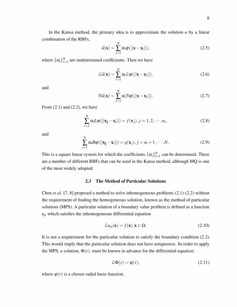
In the Kansa method, the primary idea is to approximate the solution u by a linearcombination of the RBFs,

u(x) =N

∑i=1

αiϕ(||x−xi||), (2.5)

where αiNi=1 are undetermined coefficients. Then we have

Lu(x) =N

∑i=1

αiLϕ(||x−xi||), (2.6)

and

Bu(x) =N

∑i=1

αiBϕ(||x−xi||). (2.7)

From (2.1) and (2.2), we have

N

∑i=1

αiLϕ(||xj−xi||) = f (x j), j = 1,2, · · · ,ni, (2.8)

andN

∑i=1

αiBϕ(||xj−xi||) = g(x j), j = ni +1, · · · ,N. (2.9)

This is a square linear system for which the coefficients αiNi=1 can be determined. There

are a number of different RBFs that can be used in the Kansa method, although MQ is oneof the most widely adopted.

2.3 The Method of Particular Solutions

Chen et al. [7, 8] proposed a method to solve inhomogeneous problems (2.1)-(2.2) withoutthe requirement of finding the homogeneous solution, known as the method of particularsolutions (MPS). A particular solution of a boundary value problem is defined as a functionup which satisfies the inhomogeneous differential equation

Lup(x) = f (x),x ∈Ω. (2.10)

It is not a requirement for the particular solution to satisfy the boundary condition (2.2).This would imply that the particular solution does not have uniqueness. In order to applythe MPS, a solution, Φ(r), must be known in advance for the differential equation:

LΦ(r) = ϕ(r), (2.11)

where ϕ(r) is a chosen radial basis function.

9

We can construct a particular solution up(x) in (2.10) by interpolating the forcing termf (x) using RBFs, ϕ(r),

f (x) =ni

∑i=1

αiϕ(||x−xi||). (2.12)

By (2.11), an approximate particular solution of (2.10) can be written as

up(x) =ni

∑i=1

αiΦ(||x−xi||). (2.13)

The coefficients αiNi=1 can then be determined by the same collocation technique described

in the previous section.Since the differential operator and the RBFs are radially invariant, the solutions Φ(r)

must also be radially invariant. Thus, the MPS is a special kind of RBF collocation method.Unlike the Kansa method using ϕ(r), the MPS uses Φ(r). This is an important tool forevaluating solutions of PDEs. The primary difference between the MPS and Kansa methodis the utilization of the RBF, ϕ(r), as a basis for the Kansa method, while the MPS uses thesolution of (2.11) as the basis function. While it is necessary to find the closed form of Φ

for different operators, deriving Φ(r) for higher order differential operators has proved to bea challenge. Also, this closed form depends on the dimension of the domain space.

2.4 Radial Basis Function Differential Quadrature Method

In this section, the radial basis function differential quadrature (RBF-DQ) method is pre-sented. The differential quadrature (DQ) method is a numerical discretization techniquethat approximates the derivative of a function f (x) with respect to a coordinate using alinear combination of function values in the domain of that coordinate direction as shownin [1]. The idea of the DQ method came from the integral quadrature, where the integralover a closed domain is approximated by a linear combination of function values at allnodes, such as the well known Trapezoidal Rule and Simpson’s Rule that students learnin an introductory Calculus course. A variety of methods have been developed based onthe DQ method, including the polynomial-based differential quadrature (PDQ) and theFourier-expansion-based differential quadrature (FDQ) [51, 49]. In the PDQ, the coeffi-cients are determined by a simple algebraic formulation or a recurrence relationship that isindependent of the selection of the nodal points. In a similar approach, the FDQ uses theFourier series expansion to approximate the function. While the PDQ and FDQ methods areable to obtain accurate results using only a small number of grid points, they are mesh-basedmethods. Moreover, the distribution of the nodes has limitations, and the mesh must beclustered close to the boundary limiting its usefulness.

10

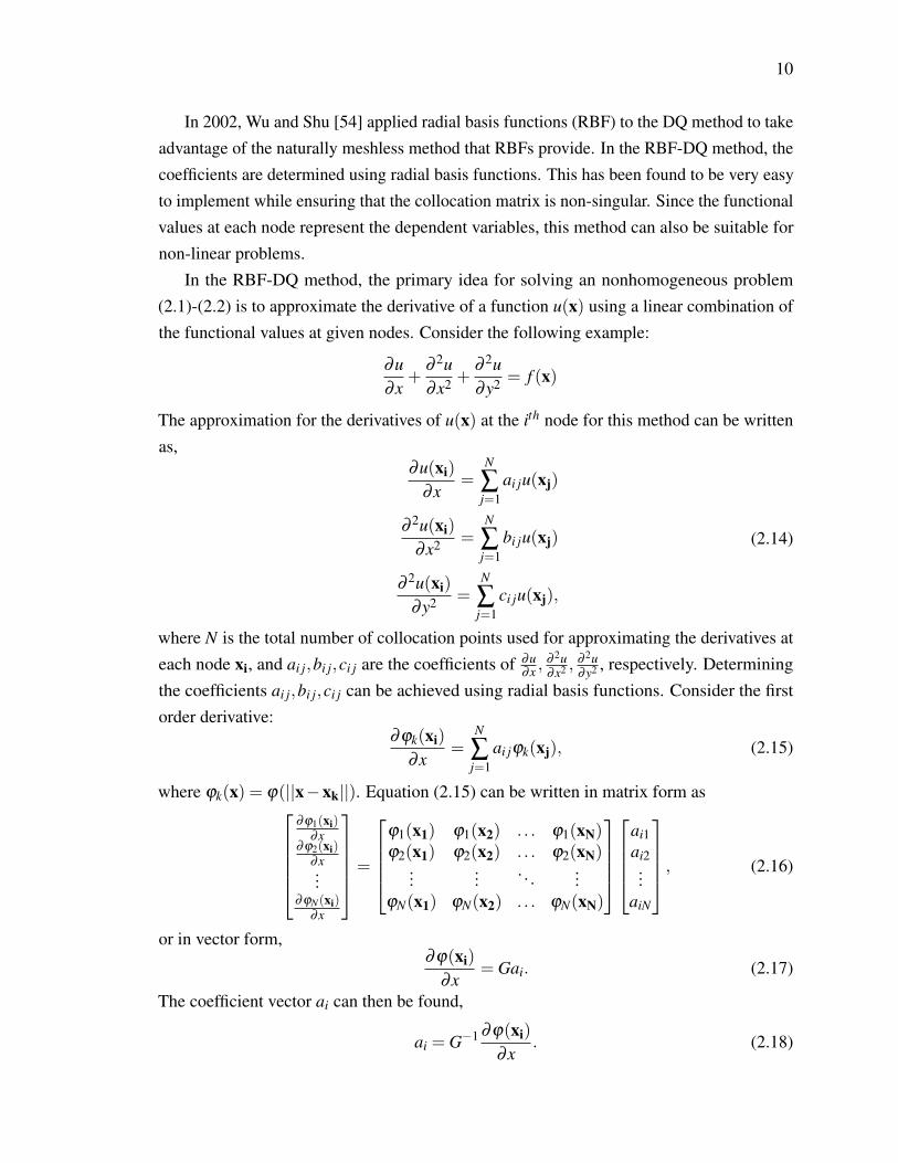
In 2002, Wu and Shu [54] applied radial basis functions (RBF) to the DQ method to takeadvantage of the naturally meshless method that RBFs provide. In the RBF-DQ method, thecoefficients are determined using radial basis functions. This has been found to be very easyto implement while ensuring that the collocation matrix is non-singular. Since the functionalvalues at each node represent the dependent variables, this method can also be suitable fornon-linear problems.

In the RBF-DQ method, the primary idea for solving an nonhomogeneous problem(2.1)-(2.2) is to approximate the derivative of a function u(x) using a linear combination ofthe functional values at given nodes. Consider the following example:

∂u∂x

+∂ 2u∂x2 +

∂ 2u∂y2 = f (x)

The approximation for the derivatives of u(x) at the ith node for this method can be writtenas,

∂u(xi)

∂x=

N

∑j=1

ai ju(xj)

∂ 2u(xi)

∂x2 =N

∑j=1

bi ju(xj)

∂ 2u(xi)

∂y2 =N

∑j=1

ci ju(xj),

(2.14)

where N is the total number of collocation points used for approximating the derivatives ateach node xi, and ai j,bi j,ci j are the coefficients of ∂u

∂x ,∂ 2u∂x2 ,

∂ 2u∂y2 , respectively. Determining

the coefficients ai j,bi j,ci j can be achieved using radial basis functions. Consider the firstorder derivative:

∂ϕk(xi)

∂x=

N

∑j=1

ai jϕk(xj), (2.15)

where ϕk(x) = ϕ(||x−xk||). Equation (2.15) can be written in matrix form as∂ϕ1(xi)

∂x∂ϕ2(xi)

∂x...

∂ϕN(xi)∂x

=

ϕ1(x1) ϕ1(x2) . . . ϕ1(xN)ϕ2(x1) ϕ2(x2) . . . ϕ2(xN)

...... . . . ...

ϕN(x1) ϕN(x2) . . . ϕN(xN)

ai1ai2...

aiN

, (2.16)

or in vector form,∂ϕ(xi)

∂x= Gai. (2.17)

The coefficient vector ai can then be found,

ai = G−1 ∂ϕ(xi)

∂x. (2.18)

11

The RBF-DQ method inherits the attractive quality from ϕ(||x−x j||) that G will alwaysbe invertible, so there is no question whether or not G is singular. Also, it is important toobserve that the matrix G is independent of xi so the coefficients at each center can easily befound by simply changing the vector ∂ϕ(xi)

∂x . Also, since G is fixed, it is only necessary tocompute this collocation matrix once and then use it to solve for the remaining coefficients,bi j and ci j. Once the coefficients have been computed using Eq. (2.14)-(2.18), it is nowpossible to solve for u,

N

∑j=1

ai ju(xj)+N

∑j=1

bi ju(xj)+N

∑j=1

ci ju(xj) = f (xi). (2.19)

By rearranging this can be written as

N

∑j=1

(ai j +bi j + ci j)u(xj) = f (xi) (2.20)

or in vector form,Au = f , (2.21)

where

A =

a11 +b11 + c11 a12 +b12 + c12 · · · a1N +b1N + c1Na21 +b21 + c21 a22 +b22 + c22 · · · a2N +b2N + c2N

......

...aN1 +bN1 + cN1 aN2 +bN2 + cN2 · · · aNN +bNN + cNN

.

By solving the above system, u can now be found.The coefficients are dependent only on the chosen RBFs, which means that it is necessary

to compute them only once. Furthermore, the RBF-DQ scheme does not require a mesh andis not sensitive to the spatial dimension, making it a multi-dimensional meshless method forsolving PDEs.

2.5 Local Radial Basis Function Differential Quadrature Method

In the global RBF-DQ method, the RBFs are used to obtain the coefficients so that thederivatives of a function f (x) can be written as a linear combination of the functional valuesat the predetermined nodes. This numerical scheme is simple and effective. However,the approximation can become unstable as the number of collocation points become largeresulting in dense matrices. This leads to ill-conditioning and sensitivity to the shapeparameters in the RBF formulation. We can alleviate these issues by using a localizedformulation. A number of RBF collocation methods have been localized, including the Kansa

12

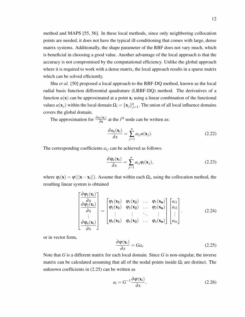
method and MAPS [55, 56]. In these local methods, since only neighboring collocationpoints are needed, it does not have the typical ill-conditioning that comes with large, densematrix systems. Additionally, the shape parameter of the RBF does not vary much, whichis beneficial in choosing a good value. Another advantage of the local approach is that theaccuracy is not compromised by the computational efficiency. Unlike the global approachwhere it is required to work with a dense matrix, the local approach results in a sparse matrixwhich can be solved efficiently.

Shu et al. [50] proposed a local approach to the RBF-DQ method, known as the localradial basis function differential quadrature (LRBF-DQ) method. The derivatives of afunction u(x) can be approximated at a point xi using a linear combination of the functionalvalues u(x j) within the local domain Ωi = x jn

j=1. The union of all local influence domainscovers the global domain.

The approximation for ∂uk(xi)∂x at the ith node can be written as:

∂uk(xi)

∂x=

n

∑j=1

ai ju(x j). (2.22)

The corresponding coefficients ai j can be achieved as follows:

∂ϕk(xi)

∂x=

n

∑j=1

ai jϕi(x j), (2.23)

where ϕi(x) = ϕ(||x−xi||). Assume that within each Ωi, using the collocation method, theresulting linear system is obtained

∂ϕ1(xi)

∂x∂ϕ2(xi)

∂x...

∂ϕn(xi)

∂x

=

ϕ1(x1) ϕ1(x2) . . . ϕ1(xn)ϕ2(x1) ϕ2(x2) . . . ϕ2(xn)

...... . . . ...

ϕn(x1) ϕn(x2) . . . ϕn(xn)

ai1ai2...

ain

. (2.24)

or in vector form,∂ϕ(xi)

∂x= Gai. (2.25)

Note that G is a different matrix for each local domain. Since G is non-singular, the inversematrix can be calculated assuming that all of the nodal points inside Ωi are distinct. Theunknown coefficients in (2.25) can be written as

ai = G−1 ∂ϕ(xi)

∂x, (2.26)

13

where

ai =

ai1ai2...

ain

and

∂ϕ(xi)

∂x=

∂ ϕ1(xi)

∂x∂ ϕ2(xi)

∂x...

∂ ϕn(xi)

∂x

.

The vectors ai, i = 1, ...,N, contain all of the required coefficients for the approximationsu(xi)N

i=1 in the global system. However, it is necessary to distribute ai appropriatelyin the global matrix. This can be accomplished by padding ai with zero entries at theappropriate positions yielding the vector α [57]. For example, suppose that N = 100, n = 3,and Ωi = x18,x26,x32. Then 97 zeros are inserted into the n-vector, ai, given in (2.26).This will pad the vector at all positions except 18, 26, and 32, as shown in

α(x) = [0,0, · · · , a1︸︷︷︸18th

,0,0, a2︸︷︷︸26th

,0,0,0, a3︸︷︷︸32nd

,0, · · · , 0︸︷︷︸100th

]. (2.27)

In (2.27) there are 17 zeros before a1 and 68 zeros after a3. This zero padding keeps trackof the original position at each local point so that α can be easily obtained from ai. This canbe repeated to solve for any of the remaining coefficients as necessary, such as bi j,ci j. Theassembly of all equations for the N centers xi will yield the N×N system

Au = f , (2.28)

where the global matrix A is sparse. The above sparse system can now be solved toapproximate u(x).

This local method is effective for solving large-scale problems. By pairing this methodwith the matrix decomposition algorithm, additional computational savings can be realizedas will be demonstrated in Chapter 5.

2.6 Shape Parameter

In the previous sections, the global and local RBF-DQ schemes were described in detail.It is important to note that this scheme is appropriate only if the collocation matrix, G,is invertible in (2.17) so that the coefficients ai can be obtained. Schoenberg [47] proved

14

the invertibility of the collocation matrix for positive definite RBFs, Gaussian, and InverseMultiquadric (IMQ). Multiquadric (MQ) is only conditionally positive definite. However, itis conditionally positive definite of order one, which Micchelli established the invertibilityof G for this class of RBFs [42]. He further proved the invertibility of the collocation matrixfor conditionally positive definite functions of order m given certain requirements, suchas polyharmonic splines. The interpolation matrix of this class of RBFs can be singulareven for non-trivial sets of distinct centers. To guarantee invertibility, it is necessary to addpolynomial terms to the RBF interpolation problem.

Among the RBFs, the multiquadric (MQ) is perhaps the most popular that is used inapplications. This is due to its high convergence rate and accuracy. Perhaps a disadvantagethat the MQ has, compared to the polyharmonic splines, is that the accuracy depends onthe correct choice of the shape parameter. This same disadvantage applies to the inversemultiquadric (IMQ) and the Gaussian (GA) RBF as well. Finding the appropriate shapeparameter that minimizes the approximation error is not trivial and is an ongoing researchproblem. In 2001, Main-Duy and Tran-Cong [40] claimed that the shape parameter relatesto the grid distance. However, other researchers such as Zhang et al. in [58] argue that theoptimal shape parameter is dependent upon the problem itself. In 2003, Lee et al. [35]claimed that the numerical solution is less sensitive to the selection of the shape parameterin the local collocation methods than the global methods. A number of different techniqueshave been developed throughout RBF literature for finding an optimal shape parameter. Ofcourse, the simplest strategy is the trial and error method where the best value of the shapeparameter is found by performing a number of experiments with different shape parametervalues. This method is certainly not sophisticated and can only be used with certainty if weknow the original function. In one of the earliest papers on the topic of RBFs, Hardy [20]suggested the value c = 1/(0.815d), where d = 1/N ∑

Nj=1 d j and d j is the distance of the jth

data value from its nearest neighbor. Franke, in 1982, [19] recommended an alternative valueof c = 0.8

√N/D, where D is the diameter of the smallest circle containing the data points

xNj=1, for the MQ RBF. Both approaches yielded satisfactory approximations. However, at

that time, only single precision computers were used. Today, double precision computationhas caused these shape parameter estimates to become obsolete.

More recently, Fasshauer [16] proposed the value c = 2√

N for interpolation in a regulardomain two dimensional problem. Fasshauer later suggested a "safe" shape parameter basedon Schaback’s uncertainty principle [15], which states that it is impossible to achieve bothgood stability and small errors simultaneously. As the shape parameter approaches zero,the coefficient matrix’s condition number grows exponentially. In this strategy, Fasshauerused the smallest value of the shape parameter without MATLAB issuing a warning of

15

ill-conditioning. While this strategy will not result in an optimal shape parameter, it does atleast guarantee that the system will not be near-singular. Rippa [45] used the Leave-One-Out-Cross-Validation (LOOCV) method to find a sub-optimal shape parameter that resultsin an accurate approximation while maintaining matrix stability. LOOCV is a techniquethat has been used extensively in RBF literature. In a large scale global scheme, LOOCVbecomes ineffective due to the great computational burden it causes. However, it can stillpresent usefulness in a local scheme, such as the local RBF-DQ. The next sections thesetechniques for calculating the shape parameter in more detail.

2.6.1 Fasshauer Estimate

For a large scale problem, the LOOCV is not a practical tactic for finding an optimalshape parameter in a global scheme. Therefore, a more sophisticated method for the shapeparameter is desired that will produce high accuracy while being able to handle a largenumber of collocation points. After extensive experimentation, Karageorghis et al. [29]observed that the value c = 4

√n/5, where n is the number of collocation points, yielded

the most accurate results when using the normalized MQ RBF. Taking this formula a stepfurther, we can allow the denominator to be adjustable, c = 4

√n/mx, where mx depends on

the density of the collocation points. As we will observe in the numerical results, as thenumber of collocation points increases, the proper value of mx decreases. Not only does thisformula yield accurate results, it is computationally simple and works well for large scaleproblems as will be shown in Chapter 5, in addition to a detailed description of how mx ischosen in the formula.

2.6.2 Leave-One-Out Cross Validation

Cross validation is a statistical technique that tests the accuracy of a method by separatinggiven data into two sections. The first section of the data set is used to calculate anapproximation of the data. The error is then measured by finding the difference between theapproximation and the actual data in the second section of the data. Leave-one-out crossvalidation (LOOCV) uses n−1 of the available n data points for the approximation. Theremaining data point is then used to calculate the error. This procedure is then repeated foreach data point, and the set of errors resulting from the n procedures are used to estimate therelative accuracy. This can be accomplished without the need of computing all of the partialinterpolants.

In order to use LOOCV to calculate the optimal shape parameter, first, define the vectorof data points with the kth data point removed x[k] = [x1,x2, ...,xk−1,xk+1, ...,xn]

T . The

16

approximation of the deleted point xk can then be found,

u[k](x) =n−1

∑i=1

αiϕi(x[k]). (2.29)

The error between the approximation and the actual value at xk can be calculated as

ek = |u(xk)− u[k](xk)|. (2.30)

The accuracy for the entire data can then be found as the norm of the vector of errorse = [e1,e2, ...,en]

T by removing each of the data points and comparing the approximationwith the exact value at the removed data point. The norm of the error vector ||e|| is the costfunction of the shape parameter. We can then choose the appropriate shape parameter thatminimizes ||e||.

This procedure would not be efficient if these n linear systems had to be solved andwould, in fact, increase the computational complexity of the RBF-DQ algorithm. However,this can be done efficiently without the need of calculating the error at every point. Rippa[45] showed that the error can be calculated using the formula

ek =αk

A−1k

, (2.31)

where αk is the kth coefficient of u for the entire data set and A−1k is the kth diagonal element

of the inverse of the corresponding interpolation matrix. Once e is calculated using the aboveformula, the relative minimum of the cost function for c can be found using the MATLABfunction fminbnd. The calling sequence for the cost function is

c = f minbnd(@(c) costeps(c,rb f ,DM,rhs),minc,maxc), (2.32)

where DM is the distance matrix of A, minc, maxc is the interval used to search for thesub-optimal shape parameter c and rhs represents the right-hand side of the equation Ax = b.While this technique provides good results, the shape parameter is not necessarily optimalbecause of its dependence on the chosen search interval (minc, maxc). The LOOCV isshown to be effective for the local RBF-DQ method, however, for the global case of largescale problems, this algorithm proves to be computationally complex. Thus, it is necessaryto present other techniques for finding an effective shape parameter.

2.6.3 Dimensionless Shape Parameter

While using a single shape parameter value for each local domain is acceptable, a secondapproach for calculating the shape parameter involves choosing a fixed value and multiplying

17

by the maximal distance in each local domain, allowing a tailored shape parameter for eachdomain. In [35], the authors found the choice of the shape parameter of MQ in the localcollocation method to be less sensitive than in the global method. The optimal shapeparameter seems to depend on the density of nodes, the number of nodes, and the functionalvalue of the nodes in the influence domain. In the LRBF-DQ method, the number of nodesin the local domain is fixed. Assigning different values of the shape parameter for eachlocal domain proves to be very difficult. In [53], the author adopted a dimensionless shapeparameter for a local collocation method to reduce this difficulty. This technique producedexcellent results using MQ. Let

r0 = max1≤ j≤n||x0−x j||, (2.33)

where r0 is the maximum distance from the center x0 to all nodal points among all localdomains Ωi, i = 1,2, ...,N as shown in Figure 2.1.

Figure 2.1: Choosing r0 in each local influence domain.

By using the dimensionless shape parameter, the MQ RBF is changed to the followingform

ϕ(r) =√

r2 +(cr0)2. (2.34)

When r0 is small, a large value for c is chosen. Overall, the desire is to select the value c

such that cr0 is a fixed number for various values of r0. This approach is also appropriate forother RBFs, such as the normalized MQ (NMQ). The NMQ RBF would then be convertedto the form

ϕ(r) =√

1+(cr0)2r2, (2.35)

Choosing the dimensionless shape parameter c becomes less critical due to the widerrange of values that will result in an accurate estimation. This makes it easier to choose ashape parameter without sacrificing accuracy. A comparison of the dimensionless shapeparameter with the LOOCV for the LRBF-DQ method will be presented in Chapter 5.

18

Chapter 3

MATRIX DECOMPOSITION ALGORITHM

In this section, the matrix decomposition algorithm (MDA) is presented. An MDA [3] is adirect method that can be used to reduce the solution of an algebraic problem into the solutionof a set of independent systems having lower dimension, leading to significant memoryand computational cost savings. For large scale problems, it is necessary to diagonalizethe coefficient matrix to alleviate the computational burden. The fact that the coefficientmatrix, as well as the right hand side matrix, are circulant yields the ability to use a FastFourier Transform to complete the diagonalization. MDAs have been successfully appliedin a variety of RBF techniques [28, 30, 31, 39].

3.1 Matrix Decomposition

Two matrices having the same eigenvalues are known as similar matrices. The eigenvaluesof an n×n matrix A are the zeros of its characteristic polynomial P(x) = det(A− xI). Ann×n matrix B such that B = S−1AS, where S is a nonsingular n×n matrix, will have thesame characteristic polynomial as A. This implies that A and B have the same eigenvalues,in other words, A and B are similar. The computational time for solving a matrix equation,such as Ax = b, can be reduced if we can diagonalize the matrix A due to the sparsity of adiagonal matrix.

If A is diagonalizable, instead of using the full matrix to solve the equation

Ax = b, (3.1)

A can be diagonalized, and (3.1) can be rewritten as

(S−1AS)(S−1x) = S−1b (3.2)

Ax = b, (3.3)

where A = S−1AS, x = S−1x, b = S−1b. The new equation (3.3) can now be solved, and thesolution to the original equation (3.1) can be recovered:

x = A−1b (3.4)

19

x = Sx. (3.5)

As the size of matrix A gets large, significant computational time can be saved using thediagonalization process. As mentioned earlier, it is necessary to possess a diagonalizablematrix in order for this process to work. In this dissertation, the matrices that are being usedare circulant. The next sections will demonstrate how to construct a circulant matrix andwill prove that all circulant matrices are diagonalizable. Details for finding the matrix S willalso be provided.

3.1.1 The domain

The domain that is being studied for the elliptic boundary value problems in this dissertationis the annulas Ω defined by

Ω =

x ∈ R2 : γ1 < ||x||< γ2. (3.6)

The boundary is ∂Ω = ∂Ω1∪∂Ω2, ∂Ω1∩∂Ω2 = /0, where ∂Ω1 =

x ∈ R2 : ||x||= γ1

and∂Ω2 =

x ∈ R2 : ||x||= γ2

. The outward unit normal vector to the boundary is denoted by

n = (nx,ny).

Figure 3.1: Annulus Domain

3.1.2 Distribution of Collocation Points

The collocation points xmnM,Nm=1,n=1 will be placed on concentric circles in the domain Ω.

First, define the M angles on each concentric circle

θm =2π(m−1)

M, m = 1, . . . ,M, (3.7)

and the radii for the N concentric circles

rn = γ1 +(γ2− γ1)n−1N−1

, n = 1, . . . ,N. (3.8)

20

For the two-dimensional case, xmnM,Nm=1,n=1 = (xmn,ymn)M,N

m=1,n=1 are then defined asfollows:

xmn = rn cos(

θm +2παn

M

), ymn = rn sin

(θm +

2παn

M

), m = 1, . . . ,M, n = 1, . . . ,N.

(3.9)The parameters αnN

n=1 ∈ [−1/2,1/2] correspond to rotations of the collocation points andmay be used to produce more uniform distributions. Typical distributions of collocationpoints without rotation (αn = 0,n = 1, ...,n) and with rotation are given in Figure 3.2.

Figure 3.2: Discretization of the annuluar domain with (a) no rotation of the collocationpoints and (b) with rotation of the collocation points. The crosses (+) denote the collocationpoints.

With the distribution of collocation points, the RBF interpolation matrix can then beconstructed. First define ϕim(r jn)=ϕ(||x jn−xim||), where i, j are the concentric circle indexand m,n are the collocation point index on each concentric circle. Then the interpolationmatrix of each ith, jth concentric circle is

Ai j =

ϕi1(r j1) ϕi1(r j2) · · · ϕi1(r jM)ϕi2(r j1) ϕi2(r j2) · · · ϕi2(r jM)

......

...ϕiM(r j1) ϕiM(r j2) · · · ϕiM(r jM)

, i, j = 1, ...,N. (3.10)

To study the effect the distribution of points will have on the interpolation matrix,

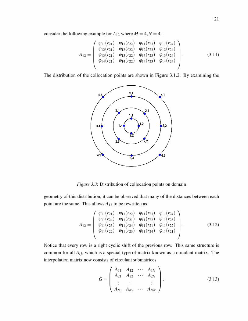
21

consider the following example for A12 where M = 4,N = 4:

A12 =

ϕ11(r21) ϕ11(r22) ϕ11(r23) ϕ11(r24)ϕ12(r21) ϕ12(r22) ϕ12(r23) ϕ12(r24)ϕ13(r21) ϕ13(r22) ϕ13(r23) ϕ13(r24)ϕ14(r21) ϕ14(r22) ϕ14(r23) ϕ14(r24)

. (3.11)

The distribution of the collocation points are shown in Figure 3.1.2. By examining the

Figure 3.3: Distribution of collocation points on domain

geometry of this distribution, it can be observed that many of the distances between eachpoint are the same. This allows A12 to be rewritten as

A12 =

ϕ11(r21) ϕ11(r22) ϕ11(r23) ϕ11(r24)ϕ11(r24) ϕ11(r21) ϕ11(r22) ϕ11(r23)ϕ11(r23) ϕ11(r24) ϕ11(r21) ϕ11(r22)ϕ11(r22) ϕ11(r23) ϕ11(r24) ϕ11(r21)

. (3.12)

Notice that every row is a right cyclic shift of the previous row. This same structure iscommon for all Ai j, which is a special type of matrix known as a circulant matrix. Theinterpolation matrix now consists of circulant submatrices

G =

A11 A12 · · · A1NA21 A22 · · · A2N

......

...AN1 AN2 · · · ANN

. (3.13)

22

In the next section, the circulant matrix will be discussed in further detail and its importancein the matrix decomposition algorithm.

3.2 Circulant Matrices

A circulant matrix occurs when every row of the matrix is a right cyclic shift of the previousrow:

CM =

c1 c2 c3 . . . cMcM c1 c2 . . . cM−1

cM−1 cM c1 . . . cM−2...

...... . . . ...

c2 c3 c4 . . . c1

(3.14)

Circulant matrices and their properties have been well documented in [13]. One advan-tage of circulant matrices is that they can be completely described by the first row of thematrix due to its cyclic permutations of the row. By strategically choosing the collocationpoints so that they lie on concentric circles, the collocation matrix will then consist ofcirculant submatrices. These circulant matrices come with special inherent properties thatcan be utilized in simplifying the process of the numerical solution to the partial differentialequation.

First, a circulant matrix can be diagonalized by a discrete Fourier transform. Letω = e2πi/M,M ≥ 1, i2 =−1. Note that ω is a primitive Mth root of unity, meaning ωM = 1.We can then construct the Fourier matrix of order M:

UM =1√M

1 1 1 · · · 11 ω ω2 · · · ωM−1

1 ω2 ω4 · · · ω2(M−1)

......

......

1 ωM−1 ω2(M−1) · · · ω(M−1)(M−1)

. (3.15)

Theorem 1. The Discrete Fourier matrix, UM, is unitary, i.e. UMU∗M = IM, where U∗M isthe conjugate transpose of UM.

Proof. Consider an element ui j of UMU∗M,

ui j =M−1

∑k=0

1√M

ωki 1√

Mω−k j =

1M

M−1

∑k=0

ωk(i− j) =

1M

(1−ωM(i− j)

1−ω i− j

). (3.16)

For i = j,

ui j =1M

(1+ω

(i− j)+ω2(i− j)+ ...+ω

(M−1)(i− j))= 1 (3.17)

23

For i 6= j,

ui j =1M

(1−ωM(i− j)

1−ω i− j

)= 0 (3.18)

Therefore, UMU∗M = IM.The eigenvalues and eigenvectors of a circulant matrix can be found by the following

equation c1 c2 c3 . . . cMcM c1 c2 . . . cM−1

cM−1 cM c1 . . . cM−2...

...... . . . ...

c2 c3 c4 . . . c1

1

ω i

ω2i

...ω(M−1)i

= λi

1

ω i

ω2i

...ω(M−1)i

, (3.19)

where i = 0, ...,M−1.

Definition 3.2.1. λi = c1 + c2ω i + ...+ cMω(M−1)i is an eigenvalue of CM.xi = [1,ω i,ω2i, ...,ω(M−1)i] is an eigenvector of CM.

Note that the columns of xiM−1i=0 of the discrete Fourier matrix, UM, are the eigenvec-

tors of CM and are independent of the entries c1, ...,cM. Hence, UM can now be used todiagonalize CM along with Λ, which is the diagonal matrix consisting of the eigenvaluesλiM−1

i=0 as the diagonal entriesCM =U∗MΛUM. (3.20)

Since UM is unitary, Λ can be written as

Λ =UMCMU∗M. (3.21)

In MATLAB, the diagonalization process can be achieved using the functions fft (fastFourier Transform) and ifft (inverse fast Fourier Transform). The fast Fourier Transform is avery efficient algorithm that is used to compute the discrete Fourier Transform by factorizingthe DFT matrix into a product of sparse factors. Using these commands not only addssavings in computational cost, but it also provides considerable savings in storage since theeigenvalues can be found using only the first row of the matrix [c1,c2, ...,cn].

To apply the diagonalization to each submatrix in the interpolation matrix (3.13), thetensor product can be applied:

A⊗B =

a11B a12B · · · a1nBa21B a22B · · · a2nB

......

...am1B am2B · · · amnB

, (3.22)

24

where A and B are m× n and p× q matrices, respectively. The resultant matrix will bemp×nq. By multiplying G, consisting of circulant submarices, by IN⊗UM on the left handside and IN⊗U∗M on the right hand side, each circulant block will be diagonalized

Λ = (IN⊗UM)G(IN⊗U∗M)

=

UM 0 · · · 00 UM · · · 0...

......

0 0 · · · UM

A11 A12 · · ·A1NA21 A22 · · ·A2N

......

...AM1 AM2 · · ·AMN

U∗M 0 · · · 00 U∗M · · · 0...

......

0 0 · · · U∗M

=

Λ11 Λ12 · · · Λ1NΛ21 Λ22 · · · Λ2N

......

...ΛM1 ΛM2 · · · ΛMN .

(3.23)

Λ is a sparse matrix consisting of diagonal submatrices.

3.3 Properties of Circulant Matrices

The following theorems will present additional properties of circulant matrices that arenecessary for the implementation of the matrix decomposition algorithm in the RBF-DQmethod.

Theorem 2. Consider the system

BA =C, (3.24)

where the MN×MN matrices B and C are block circulant, each consisting of N2 circulant

submatrices Bn1,n2,Cn1,n2,n1,n2 = 1, . . . ,N, respectively, each of order M. Assume that the

matrix B is nonsingular. Then the MN×MN matrix A will also be block circulant consisting

of N2 circulant submatrices An1,n2,n1,n2 = 1, . . . ,N, each of order M.

Proof. It is first necessary to prove that if an MN×MN matrix B is block circulant then sois its inverse. Since B is block circulant, B can be rewritten as

B = (IN⊗U∗M)D(IN⊗UM) , (3.25)

where the matrix D is block diagonal and nonsingular, consisting of N2 diagonal submatricesDn1,n2,n1,n2 = 1, . . . ,N, each of order M. The inverse of the matrix B will be

B−1 = (IN⊗U∗M)D−1 (IN⊗UM) . (3.26)

25

Next, it must be proven that since D is block diagonal, so is D−1. Let D−1 consist of N2

submatrices Dn1,n2 ,n1,n2 = 1, . . . ,N, each of order M. ThenD1,1 D1,2 · · · D1,ND2,1 D2,2 · · · D2,N

......

...DN,1 DN,2 · · · DN,N

D1,1 D1,2 · · · D1,ND2,1 D2,2 · · · D2,N

......

...DN,1 DN,2 · · · DN,N

=

IM 0 · · · 00 IM · · · 0...

......

0 0 · · · IM

,

(3.27)where each diagonal submatrix Dn1,n2 = diag

(dn1,n2

1 ,dn1,n22 , . . . ,dn1,n2

M). Assume that each

submatrix Dn1,n2 =(dn1,n2

m1,m2

)Mm1,m2=1, is full.

Consider the system created by multiplying D by the first column of D−1D1,1 D1,2 · · · D1,ND2,1 D2,2 · · · D2,N

......

...DN,1 DN,2 · · · DN,N

D1,1D2,1

...DN,1

=

IM0...0

. (3.28)

This system can be broken to M independent systems of order Nd1,1

1 d1,21 · · · d1,N

1d2,1

1 d2,21 · · · d2,N

1...

......

dN,11 dN,2

1 · · · dN,N1

d1,11,1 d1,1

1,2 · · · d1,11,M

d2,11,1 d2,1

1,2 · · · d2,11,M

......

...dN,1

1,1 dN,11,2 · · · dN,1

1,M

=

1 0 · · · 00 0 · · · 0...

......

0 0 · · · 0

,

d1,1

2 d1,22 · · · d1,N

2d2,1

2 d2,22 · · · d2,N

2...

......

dN,12 dN,2

2 · · · dN,N2

d1,12,1 d1,1

2,2 · · · d1,12,M

d2,12,1 d2,1

2,2 · · · d2,12,M

......

...dN,1

2,1 dN,12,2 · · · dN,1

2,M

=

0 1 · · · 00 0 · · · 0...

......

0 0 · · · 0

,

up tod1,1

M d1,2M · · · d1,N

Md2,1

M d2,2M · · · d2,N

M...

......

dN,1M dN,2

M · · · dN,NM

d1,1M,1 d1,1

M,2 · · · d1,1M,M

d2,1M,1 d2,1

M,2 · · · d2,1M,M

......

...dN,1

M,1 dN,1M,2 · · · dN,1

M,M

=

0 0 · · · 10 0 · · · 0...

......

0 0 · · · 0

,

Similarly, the systemD1,1 D1,2 · · · D1,ND2,1 D2,2 · · · D2,N

......

...DN,1 DN,2 · · · DN,N

D1,2D2,2

...DN,2

=

0

IM0...0

, (3.29)

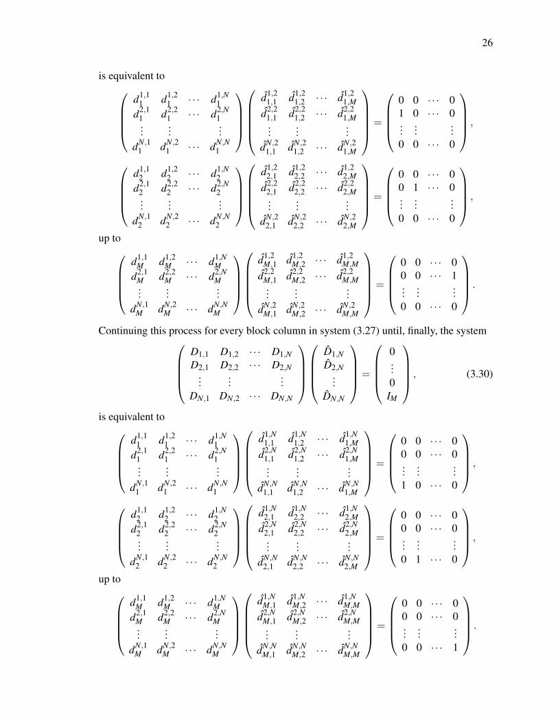
26

is equivalent tod1,1

1 d1,21 · · · d1,N

1d2,1

1 d2,21 · · · d2,N

1...

......

dN,11 dN,2

1 · · · dN,N1

d1,21,1 d1,2

1,2 · · · d1,21,M

d2,21,1 d2,2

1,2 · · · d2,21,M

......

...dN,2

1,1 dN,21,2 · · · dN,2

1,M

=

0 0 · · · 01 0 · · · 0...

......

0 0 · · · 0

,

d1,1

2 d1,22 · · · d1,N

2d2,1

2 d2,22 · · · d2,N

2...

......

dN,12 dN,2

2 · · · dN,N2

d1,22,1 d1,2

2,2 · · · d1,22,M

d2,22,1 d2,2

2,2 · · · d2,22,M

......

...dN,2

2,1 dN,22,2 · · · dN,2

2,M

=

0 0 · · · 00 1 · · · 0...

......

0 0 · · · 0

,

up tod1,1

M d1,2M · · · d1,N

Md2,1

M d2,2M · · · d2,N

M...

......

dN,1M dN,2

M · · · dN,NM

d1,2M,1 d1,2

M,2 · · · d1,2M,M

d2,2M,1 d2,2

M,2 · · · d2,2M,M

......

...dN,2

M,1 dN,2M,2 · · · dN,2

M,M

=

0 0 · · · 00 0 · · · 1...

......

0 0 · · · 0

.

Continuing this process for every block column in system (3.27) until, finally, the systemD1,1 D1,2 · · · D1,ND2,1 D2,2 · · · D2,N

......

...DN,1 DN,2 · · · DN,N

D1,ND2,N

...DN,N

=

0...0

IM

, (3.30)

is equivalent tod1,1

1 d1,21 · · · d1,N

1d2,1

1 d2,21 · · · d2,N

1...

......

dN,11 dN,2

1 · · · dN,N1

d1,N1,1 d1,N

1,2 · · · d1,N1,M

d2,N1,1 d2,N

1,2 · · · d2,N1,M

......

...dN,N

1,1 dN,N1,2 · · · dN,N

1,M

=

0 0 · · · 00 0 · · · 0...

......

1 0 · · · 0

,

d1,1

2 d1,22 · · · d1,N

2d2,1

2 d2,22 · · · d2,N

2...

......

dN,12 dN,2

2 · · · dN,N2

d1,N2,1 d1,N

2,2 · · · d1,N2,M

d2,N2,1 d2,N

2,2 · · · d2,N2,M

......

...dN,N

2,1 dN,N2,2 · · · dN,N

2,M

=

0 0 · · · 00 0 · · · 0...

......

0 1 · · · 0

,

up tod1,1

M d1,2M · · · d1,N

Md2,1

M d2,2M · · · d2,N

M...

......

dN,1M dN,2

M · · · dN,NM

d1,NM,1 d1,N

M,2 · · · d1,NM,M

d2,NM,1 d2,N

M,2 · · · d2,NM,M

......

...dN,N

M,1 dN,NM,2 · · · dN,N

M,M

=

0 0 · · · 00 0 · · · 0...

......

0 0 · · · 1

.

27

The solution of system (3.27) is equivalent to solving the systems

EmFmn = Imn, m = 1, . . . ,M, n = 1, . . . ,N,

where

Em =

d1,1

m d1,2m · · · d1,N

m

d2,1m d2,2

m · · · d2,Nm

......

...dN,1

m dN,2m · · · dN,N

m

,m = 1, ...,M,

(Fmn)i, j =(

di,nm, j

), i,n = 1, . . . ,N, j,m = 1, . . . ,M,

and Imn,m = 1, . . . ,M, n = 1, . . . ,N, are zero matrices with 1 at the position (n,m). This canbe written more compactly as M systems with MN right hand sides,

Em (Fm1|Fm2| . . . |FmN) =(Im1|Im2| . . . |ImN

), m = 1, . . . ,M. (3.31)

Since the matrix D−1 is nonsingular, each matrix Em is nonsingular, and from (3.31), foreach n = 1, . . . ,N, the only nonzero column in matrix Fmn is column m. This means thatin each submatrix Dn1,n2,n1,n2 = 1, . . . ,N, the only nonzero elements are the elements(dn1,n2

m,m)M

m=1, which implies that each submatrix Dn1,n2 is diagonal, and hence D−1 is blockdiagonal. Therefore,

B−1 = (IN⊗U∗M)D−1 (IN⊗UM) =

U∗MD1,1UM U∗MD1,2UM · · · U∗MD1,NUMU∗MD2,1UM U∗MD2,2UM · · · U∗MD2,NUM

......

...U∗MDN,1UM U∗MDN,2UM · · · U∗MDN,NUM

(3.32)

and from [13, Theorem 3.2.3] each of the matrices U∗MDn1,n2UM, n1,n2 = 1, . . . ,N, is circu-lant. Therefore B−1 is block circulant.

From (3.24),A = B−1C, (3.33)

where B−1 and C are block circulant, each consisting of N2 circulant matrices of order M.Since from [13, Theorem 3.2.4] the sum and the product of circulant matrices is circulant,it easily follows that the matrix A is block circulant, consisting of N2 circulant matrices oforder M.

Corollary 1. Consider the system

BA =C, (3.34)

28

where the MN×MN matrix B is block circulant, consisting of N2 circulant submatrices

Bn1,n2,n1,n2 = 1, . . . ,N, each of order M, and the MN ×M matrix C is block circulant,

consisting of N circulant submatrices Cn,n = 1, . . . ,N, each of order M. Assume that the

matrix B is nonsingular. Then the MN×N matrix A will also be block circulant consisting

of N circulant submatrices An,n = 1, . . . ,N, each of order M.

Proof. From Theorem 2 it follows that the inverse of matrix B in (3.34) is block circulant,consisting of N2 circulant matrices of order M. Since C is also block circulant, consisting ofN circulant submatrices Cn,n = 1, . . . ,N, each of order M, since the sum and the product ofcirculant matrices is circulant, it follows that the matrix A is block circulant, consisting of N

circulant matrices of order M.The following theorem and corollary will be necessary for solving the Cauchy Navier

elasticity problem.

Theorem 3. Consider the system(B11 B12B21 B22

)(A11 A12A21 A22

)=

(C11 C12C21 C22

), (3.35)

where the MN×MN matrices Bi j,Ci j, i, j = 1,2, are block circulant, each consisting of

N2 circulant submatrices Bi jn1,n2,C

i jn1,n2,n1,n2 = 1, . . . ,N, i, j = 1,2, respectively, each of

order M. Assume that the matrices Bi j, i, j = 1,2, are nonsingular. Then the MN×MN

matrices Ai j, i, j = 1,2, will also be block circulant consisting of N2 circulant submatrices

Ai jn1,n2,n1,n2 = 1, . . . ,N, i, j = 1,2, each of order M.

Proof. It is first necessary to prove that if the inverse of the coefficient matrix in system(3.35) is (

B11 B12B21 B22

)=

(B11 B12B21 B22

)−1

,

then each of the matrices Bi j, i, j = 1,2, is block circulant consisting of N2 circulant subma-trices of order M.

From the properties of circulant matrices it follows that(B11 B12B21 B22

)= (I2⊗ IN⊗U∗M)

(D11 D12D21 D22

)(I2⊗ IN⊗UM) , (3.36)

where each of the matrices Di j, i, j = 1,2, is block diagonal and nonsingular, consisting ofN2 diagonal submatrices each of order M. The inverse of(

B11 B12B21 B22

)

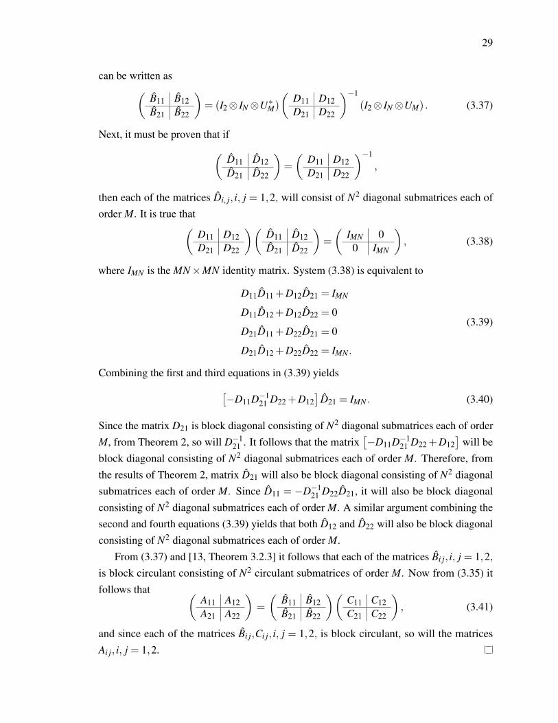
29

can be written as(B11 B12B21 B22

)= (I2⊗ IN⊗U∗M)

(D11 D12D21 D22

)−1

(I2⊗ IN⊗UM) . (3.37)

Next, it must be proven that if(D11 D12D21 D22

)=

(D11 D12D21 D22

)−1

,

then each of the matrices Di, j, i, j = 1,2, will consist of N2 diagonal submatrices each oforder M. It is true that(

D11 D12D21 D22

)(D11 D12D21 D22

)=

(IMN 0

0 IMN

), (3.38)

where IMN is the MN×MN identity matrix. System (3.38) is equivalent to

D11D11 +D12D21 = IMN

D11D12 +D12D22 = 0

D21D11 +D22D21 = 0

D21D12 +D22D22 = IMN .

(3.39)

Combining the first and third equations in (3.39) yields[−D11D−1

21 D22 +D12]

D21 = IMN . (3.40)

Since the matrix D21 is block diagonal consisting of N2 diagonal submatrices each of orderM, from Theorem 2, so will D−1

21 . It follows that the matrix[−D11D−1

21 D22 +D12]

will beblock diagonal consisting of N2 diagonal submatrices each of order M. Therefore, fromthe results of Theorem 2, matrix D21 will also be block diagonal consisting of N2 diagonalsubmatrices each of order M. Since D11 = −D−1

21 D22D21, it will also be block diagonalconsisting of N2 diagonal submatrices each of order M. A similar argument combining thesecond and fourth equations (3.39) yields that both D12 and D22 will also be block diagonalconsisting of N2 diagonal submatrices each of order M.

From (3.37) and [13, Theorem 3.2.3] it follows that each of the matrices Bi j, i, j = 1,2,is block circulant consisting of N2 circulant submatrices of order M. Now from (3.35) itfollows that (

A11 A12A21 A22

)=

(B11 B12B21 B22

)(C11 C12C21 C22

), (3.41)

and since each of the matrices Bi j,Ci j, i, j = 1,2, is block circulant, so will the matricesAi j, i, j = 1,2.

30

Corollary 2. Consider the system(A11 A12A21 A22

)(B11 B12B21 B22

)=

(C11 C12C21 C22

), (3.42)

where the MN×MN matrices Bi j, i, j = 1,2, are block circulant, each consisting of N2

circulant submatrices Bi jn1,n2,n1,n2 = 1, . . . ,N, i, j = 1,2, each of order M, and now the

MN×M matrices Ci j, i, j = 1,2, are block circulant, each consisting of N circulant subma-

trices Ci jn ,n = 1, . . . ,N, i, j = 1,2, each of order M. Assume that the MN×MN matrices

Bi j, i, j = 1,2 are nonsingular. Then the MN×M matrices Ai j, i, j = 1,2, are also block

circulant, each consisting of N circulant submatrices Ai jn ,n = 1, . . . ,N, i, j = 1,2, each of

order M.

Proof. From (3.42) it follows that(A11 A12A21 A22

)=

(B11 B12B21 B22

)(C11 C12C21 C22

)where, from Theorem 2, each of the matrices Bi j, i, j = 1,2, is block circulant consistingof N2 circulant submatrices of order M. Since each of the matrices Ci j, i, j = 1,2, is alsoblock circulant consisting of N circulant submatrices of order M, and since the sum andthe product of circulant matrices is circulant, it follows that the matrices Ai j, i, j = 1,2, areblock circulant, each consisting of N circulant matrices of order M.

31

Chapter 4

Global and Local RBF-DQ MDA

4.1 RBF-DQ MDA

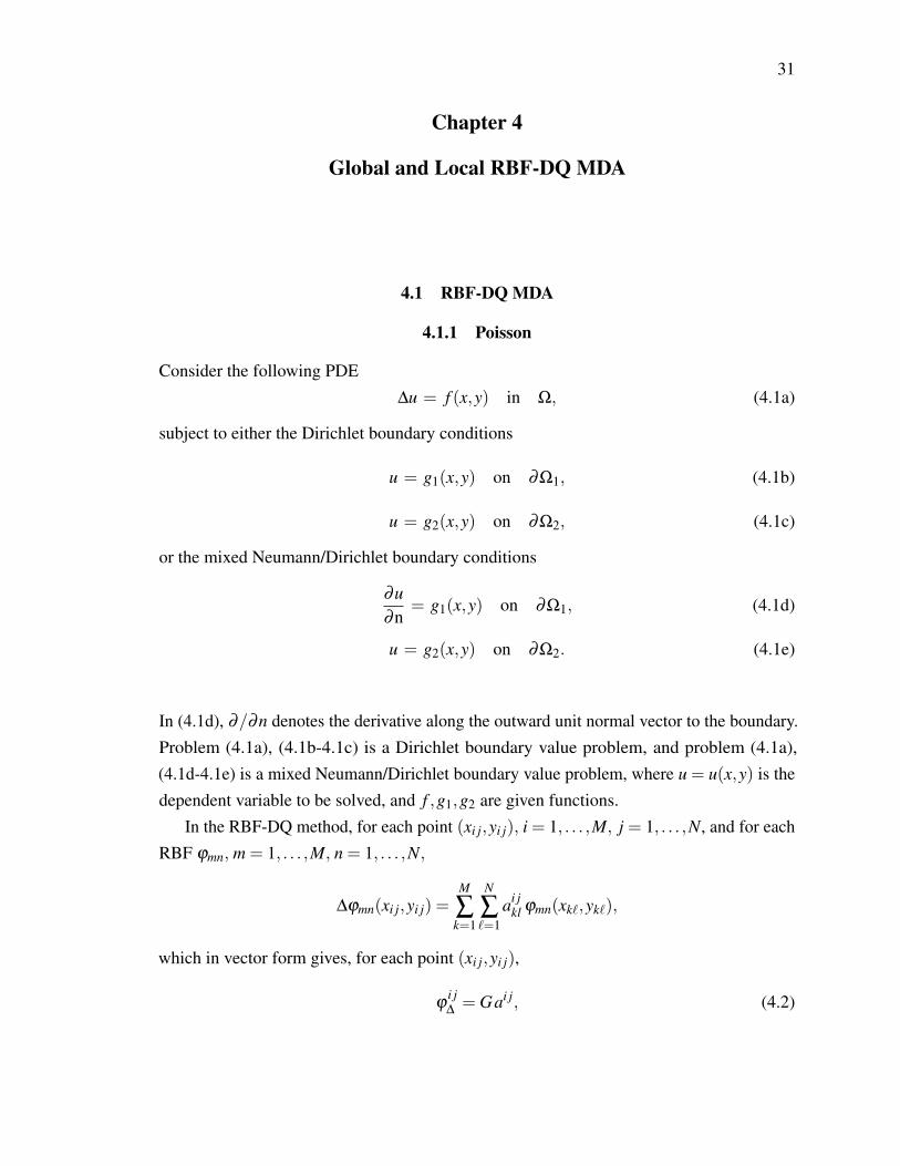
4.1.1 Poisson

Consider the following PDE∆u = f (x,y) in Ω, (4.1a)

subject to either the Dirichlet boundary conditions

u = g1(x,y) on ∂Ω1, (4.1b)

u = g2(x,y) on ∂Ω2, (4.1c)

or the mixed Neumann/Dirichlet boundary conditions

∂u∂n

= g1(x,y) on ∂Ω1, (4.1d)

u = g2(x,y) on ∂Ω2. (4.1e)

In (4.1d), ∂/∂n denotes the derivative along the outward unit normal vector to the boundary.Problem (4.1a), (4.1b-4.1c) is a Dirichlet boundary value problem, and problem (4.1a),(4.1d-4.1e) is a mixed Neumann/Dirichlet boundary value problem, where u = u(x,y) is thedependent variable to be solved, and f ,g1,g2 are given functions.

In the RBF-DQ method, for each point (xi j,yi j), i = 1, . . . ,M, j = 1, . . . ,N, and for eachRBF ϕmn, m = 1, . . . ,M, n = 1, . . . ,N,

∆ϕmn(xi j,yi j) =M

∑k=1

N

∑`=1

ai jkl ϕmn(xk`,yk`),

which in vector form gives, for each point (xi j,yi j),

ϕi j∆= Gai j, (4.2)

32

where

G =

ϕ11(r11) ϕ11(r12) ϕ11(r13) · · · ϕ11(rMN)ϕ12(r11) ϕ12(r12) ϕ12(r13) · · · ϕ12(rMN)

......

...ϕMN(r11) ϕMN(r12) ϕMN(r13) · · · ϕMN(rMN)

, (4.3)

ϕi j∆= [∆ϕ(ri j

11) ∆ϕ(ri j12) · · ·∆ϕ(ri j

MN)]T , and ai j = [ai j

11 ai j12 · · · ai j

MN ]T .

Due to the circular distribution of the collocation points, the (MN×MN) matrix G consistsof N2 circulant submatrices An1,n2,n1,n2 = 1, . . . ,N, each of order M, and is therefore blockcirculant. Moreover, the MN×MN matrix Φ =

[ϕ11

∆|ϕ12

∆|ϕ13

∆| . . . |ϕMN

∆

]also consists of

N2 circulant [13] submatrices Φn1,n2,n1,n2 = 1, . . . ,N, each of order M, and is thereforealso block circulant. It follows that, by Theorem 2 in Chapter 3, the MN×MN matrixA = [a11|a12|...aMN ] will also be block circulant, consisting of N2 circulant submatricesAn1,n2,n1,n2 = 1, ...,N, each of order M.

Equation (4.2) can be written more compactly as

GA = Φ. (4.4)

Once A = [a11|a12|...aMN ] is computed, for each point (xi j,yi j),

∆u(xi j,yi j)≈M

∑k=1

N

∑l=1

ai jklukl, (4.5)

where the ukl are approximations of u(xkl,ykl). Substitution in the differential equationyields

M

∑k=1

N

∑l=1

ai jklukl = f (xi j,yi j), i = 1, ...,M, j = 2, ...,N−1. (4.6)

In the case of the Dirichlet boundary condition,

ui1 = g1(xi1,yi1) and uiN = g2(xiN ,yiN), i = 1, ...,M. (4.7)

In the case of the Neumann/Dirichlet boundary condition, for each point (xi1,yi1), i =

1, ...,M, on the boundary ∂Ω1, and for each RBF ϕmn,m = 1, ...,M,n = 1, ...,N,

∂ϕmn

∂n(xi1,yi1) =

M

∑k=1

N

∑l=1

bi1klϕmn(xkl,ykl), (4.8)

which in vector form gives, for each boundary point (xi1,yi1) on ∂Ω1,

ϕi1n = Gbi1. (4.9)

33

The MN×M matrix Ψ = [ϕ11n |ϕ21

n |...|ϕM1n ] now consists of N circulant submatrices Φn,n =

1, ...,N, each of order M, and is therefore block circulant. It follows from Corollary 1 thatthe matrix B = [b11

n |b21n |...|bM1

n ] will also have the same block circulant structure. Equation(4.9) can be written more compactly as

GB = Ψ. (4.10)

Once B = [b11|b12|...|bMN ] is computed, for each boundary point (xi1,yi1) on ∂Ω1,

∂u∂n

(xi1,yi1)≈M

∑k=1

N

∑l=1

bi1klukl. (4.11)

So now in addition to (4.6), instead of (4.7), the equations corresponding to the boundaryconditions is written as

M

∑k=1

N

∑`=1

bi1kl uk` = g1(xi1,yi1) and uiN = g2(xiN ,yiN), i = 1, . . . ,M. (4.12)

The system can now be effectively solved using the Matrix Decomposition Algorithm asdetailed below.

4.1.2 Matrix Decomposition Algorithm

As shown in section 3.1, the system (4.2) can be premultiplied by the matrix IN⊗UM. Totake advantage of the fact that the right hand side is block circulant, the system can also bepost multiplied by the matrix IN⊗U∗M in order to diagonalize the submatrices on the righthand side for additional computational savings. The system then becomes

(IN⊗UM)G(IN⊗U∗M)(IN⊗UM)A(IN⊗U∗M) = (IN⊗UM)Φ(IN⊗U∗M) , (4.13)

orGA = Φ, (4.14)

where

G=(IN⊗UM)G(IN⊗U∗M) , A=(IN⊗UM)A(IN⊗U∗M) , Φ=(IN⊗UM)Φ(IN⊗U∗M) .

34

The matrices G and Φ are sparse block diagonal and can be calculated using the fast Fouriertransform (FFT). More specifically,

G = (IN⊗UM)G(IN⊗U∗M) =

UMG1,1U∗M UMG1,2U∗M · · · UMG1,NU∗MUMG2,1U∗M UMG2,2U∗M · · · UMG2,NU∗M

......

...UMGN,1U∗M UMGN,2U∗M · · · UMGN,NU∗M

=

G1,1 G1,2 · · · G1,NG2,1 G2,2 · · · G2,N

......

...GN,1 GN,2 · · · GN,N

, (4.15)

A = (IN⊗UM)A(IN⊗U∗M) =

UMA1,1U∗M UMA1,2U∗M · · · UMA1,NU∗MUMA2,1U∗M UMA2,2U∗M · · · UMA2,NU∗M

......

...UMAN,1U∗M UMAN,2U∗M · · · UMAN,NU∗M

=

A1,1 A1,2 · · · A1,NA2,1 A2,2 · · · A2,N

......

...AN,1 AN,2 · · · AN,N

, (4.16)

and

Φ = (IN⊗UM)Φ(IN⊗U∗M) =

UMΦ1,1U∗M UMΦ1,2U∗M · · · UMΦ1,NU∗MUMΦ2,1U∗M UMΦ2,2U∗M · · · UMΦ2,NU∗M

......

...UMΦN,1U∗M UMΦN,2U∗M · · · UMΦN,NU∗M

=

Φ1,1 Φ1,2 · · · Φ1,NΦ2,1 Φ2,2 · · · Φ2,N

......

...ΦN,1 ΦN,2 · · · ΦN,N

. (4.17)

From the properties of circulant matrices, the matrices G and Φ both consist of N2 blocks oforder M, each of which is diagonal. It follows that the matrix A will also be diagonal.

The coefficient matrix A can therefore be obtained by decomposing system (4.2) intothe M independent systems of order N

(Gn1,n2)m(An1,n2)m = (Φn1,n2)m, n1,n2 = 1, ...,N, m = 1, ...,M. (4.18)

For the mixed Neumann/Dirichlet problem, the corresponding coefficients,B = (In⊗UM)B(In⊗U∗M) can be obtained in a similar fashion. By pre-multiplying system

35

(4.9) by the matrix IN⊗UM and post-multiplying it by the matrix U∗M, the system becomes

(IN⊗UM)G(IN⊗U∗M)(IN⊗UM)BU∗M = (IN⊗UM)ΨU∗M, (4.19)

orGB = Ψ, (4.20)

where the matrix Ψ is sparse block diagonal and can be calculated using FFT. More specifi-cally,

B = (IN⊗UM)BU∗M =

UMB1U∗MUMB2U∗M

...UMBNU∗M

=

B1B2...

BN

, (4.21)

and

Ψ = (IN⊗UM)ΨU∗M =

UMΨ1U∗MUMΨ2U∗M

...UMΨNU∗M

=

Ψ1Ψ2...

ΨN

. (4.22)

The matrix G consists of N2 diagonal blocks of order M and from the properties of circulantmatrices, the matrix Ψ will consist of N blocks of order M, each of which is diagonal.In addition, since the coefficient matrix B is block circulant, consisting of N circulantsubmatrices of order M, B will consist of N diagonal blocks of order M. B can therefore beobtained by decomposing system (4.20) into solving the M independent systems of order N

(Gn1,n2)m(Bn)m = (Ψn)m, n = 1, ...,N, m = 1, ...,M. (4.23)

By appropriately arranging the matrices B (for the Neumann boundary condition) and A (forthe differential equation), the matrix A1 can be obtained to be used in the folllowing system

A1u = f , (4.24)

where u = (IN⊗UM)u and f = (IN⊗UM) f .System (4.24) is sparse block diagonal and may be solved efficiently to yield u. Finally,

u is obtained from u = (IN⊗U∗M) u. Note that all operations involving multiplication by thematrices IN⊗UM and IN⊗U∗M are carried out using the MATLAB c© [41] FFT commandsifft and fft, respectively.

36

4.1.3 Biharmonic

Consider the following biharmonic equation

∆2u = f (x,y) in Ω, (4.25a)

subject to the boundary conditions

u = g1(x,y) and∂u∂n

= h1(x,y) on ∂Ω1, (4.25b)

andu = g2(x,y) and

∂u∂n

= h2(x,y) on ∂Ω2, (4.25c)

or the boundary conditions

u = g1(x,y) and ∆u = h1(x,y) on ∂Ω1, (4.25d)

andu = g2(x,y) and ∆u = h2(x,y) on ∂Ω2. (4.25e)

Problem (4.25a),(4.25b)-(4.25c) is known as the first biharmonic problem whereas theproblem (4.25a),(4.25d)-(4.25e) is known as the second biharmonic problem.

The collocation points are defined in the same way as the previous case for the Poissonproblem. However, the interior points are defined as (xi j,yi j)

Mi=1, j = 3, · · · ,N−2, while the

boundary points are defined as (xi1,yi1)Mi=1 and (xiN ,yiN)M

i=1. Fewer interior points aretaken than in the previous case due to the fact that it is necessary to impose two boundaryconditions on the boundary instead of one in the biharmonic case. Hence, there are (N−4)Minterior points while there are 4M boundary points for a total of MN collocation points.

In the RBF-DQ method, for each point (xi j,yi j), i = 1, . . . ,M, j = 1, . . . ,N, and for eachRBF ϕmn, m = 1, . . . ,M, n = 1, . . . ,N,

∆2ϕmn(xi j,yi j) =

M

∑k=1

N

∑`=1

ai jkl ϕmn(xk`,yk`),

which in vector form, gives for each point (xi j,yi j),

ϕi j∆2 = Gai j. (4.26)

As was the case in the Poisson equation, due to the circular distribution of the collo-cation points, the matrix G is block circulant of size (MN ×MN). The matrix Φ =[ϕ11

∆2 |ϕ12∆2 |ϕ13

∆2 | . . . |ϕMN∆2

]consists of N2 circulant submatrices of order M and is therefore

37

also block circulant. This means that the matrix A =[a11|a12|a13| . . . |aMN] will also be

block circulant. Equation (4.26) can be written more compactly as

GA = Φ. (4.27)

Once A = [a11|a12|...|aMN ] is computed, for each point (xi j,yi j),

∆2u(xi j,yi j)≈

M

∑k=1

N

∑l=1

ai jklukl, (4.28)

where the ukl are approximations of u(xkl,ykl). Substitution in the differential equationyields

M

∑k=1

N

∑l=1

ai jklukl = f (xi j,yi j), i = 1, ...,M, j = 3, ...,N−2. (4.29)

In the case of the first biharmonic problem, for each boundary point (xis,yis), i= 1, . . . ,M,s = 1,N, on ∂Ω and for each RBF ϕmn, m = 1, . . . ,M, n = 1, . . . ,N,

∂ϕmn

∂n(xis,yis) =

M

∑k=1

N

∑`=1

biskl ϕmn(xk`,yk`), (4.30)

which in vector form gives for each boundary point (xis,yis),

ϕisn = Gbis. (4.31)

By observing that the MN ×M matrix Ψ =[ϕ1s

n |ϕ2sn | . . . |ϕMs

n], s = 1,N, consists of N

circulant submatrices of order M, B =[b1s|b2s| . . . |bMs], s = 1,N, is also block circulant.

Equation (4.31) can be written more compactly as

GB = Ψ. (4.32)

Once B = [b1s|b2s|...|bMs], s = 1, ...,N, is computed, for each boundary point (xis,yis), i =

1, ...,M,s = 1,N,∂u∂n

(xis,yis)≈M

∑k=1

N

∑l=1

bisklukl, (4.33)

.In the case of the second biharmonic problem, instead of (4.30), for each boundary point

(xis,yis), i = 1, . . . ,M, s = 1,N, and for each RBF ϕmn, m = 1, . . . ,M, n = 1, . . . ,N,

∆ϕmn(xis,yis) =M

∑k=1

N

∑`=1

biskl ϕmn(xk`,yk`), (4.34)

38

which in vector form gives for each boundary point (xis,yis),

ϕis∆ = Gbis. (4.35)

As in the first biharmonic problem, by observing that the matrix Ψ =[ϕ1s

∆|ϕ2s

∆| . . . |ϕMs

∆

],

s= 1,N, consists of N circulant submatrices of order M, B=[b1s|b2s| . . . |bMs], s= 1,N, will

also be block circulant. Equation (4.35) can be written more compactly as Equation (4.32).Once B = [b1s|b2s|...|bMs] is computed, for each boundary point (xis,yis), i = 1, ...,M,s =

1,N,

∆u(xis,yis)≈M

∑k=1

N

∑l=1

bisklukl. (4.36)

So now, in addition to Equation (4.29), the boundary condition (4.25b) or (4.25d) is writtenas

ui1 = g1(xi1,yi1),M

∑k=1

N

∑l=1

bi1klukl = h1(xi1,yi1), i = 1, ...,M, (4.37)

and boundary conditions (4.25c) or (4.25e) is written as

uiN = g2(xin,yin),M

∑k=1

N

∑l=1

biNkl ukl = h1(xiN ,yiN), i = 1, ...,M. (4.38)

The system can then effectively be solved using the same MDA technique as in the Poissonproblem described in the previous section.

In this dissertation, the selection of the collocation points must be determined strate-gically to achieve a circulant structure. The collocation points, (xi j,yi j), are determinedby

xmn = rn cos(

θm +2παn

M

), ymn = rn sin

(θm +

2παn

M

), m = 1, . . . ,M, n = 1, . . . ,N,

(4.39)where rn = γ1 +(γ2− γ1)

n−1N−1 is the radius of each of the N concentric circles, θm is the

angle of each of the m collocation points on a circle, and αn is the rotation of the collocatoinpoints, which is used to produce more uniform distributions. For the Poisson equation,αn = (−1)n/4,n = 1, ...,N, is used for selecting the collocation points. However, whenusing this same value for the biharmonic equation, possible singularities may occur as shownin the following theorem.

Theorem 4. For the biharmonic problems (4.25) considered, in the case αn =(−1)n/4,n=1, . . . ,N, and M = 2m is even, the global matrix G in (4.26) resulting from the proposed

discretization is singular.

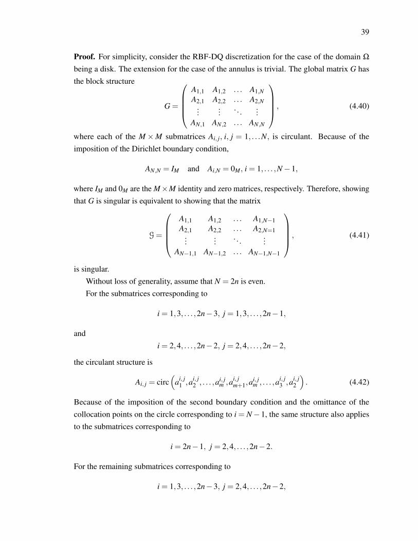
39

Proof. For simplicity, consider the RBF-DQ discretization for the case of the domain Ω

being a disk. The extension for the case of the annulus is trivial. The global matrix G hasthe block structure

G =

A1,1 A1,2 . . . A1,NA2,1 A2,2 . . . A2,N

...... . . . ...

AN,1 AN,2 . . . AN,N

, (4.40)

where each of the M×M submatrices Ai, j, i, j = 1, . . .N, is circulant. Because of theimposition of the Dirichlet boundary condition,

AN,N = IM and Ai,N = 0M, i = 1, . . . ,N−1,

where IM and 0M are the M×M identity and zero matrices, respectively. Therefore, showingthat G is singular is equivalent to showing that the matrix

G=

A1,1 A1,2 . . . A1,N−1A2,1 A2,2 . . . A2,N=1

...... . . . ...

AN−1,1 AN−1,2 . . . AN−1,N−1

, (4.41)

is singular.Without loss of generality, assume that N = 2n is even.For the submatrices corresponding to

i = 1,3, . . . ,2n−3, j = 1,3, . . . ,2n−1,

andi = 2,4, . . . ,2n−2, j = 2,4, . . . ,2n−2,

the circulant structure is

Ai, j = circ(

ai, j1 ,ai, j

2 , . . . ,ai, jm ,ai, j

m+1,ai, jm , . . . ,ai, j

3 ,ai, j2

). (4.42)

Because of the imposition of the second boundary condition and the omittance of thecollocation points on the circle corresponding to i = N−1, the same structure also appliesto the submatrices corresponding to

i = 2n−1, j = 2,4, . . . ,2n−2.

For the remaining submatrices corresponding to

i = 1,3, . . . ,2n−3, j = 2,4, . . . ,2n−2,

40

andi = 2,4, . . . ,2n−2, j = 1,3, . . . ,2n−1,

and alsoi = 2n−1, j = 1,3, . . . ,2n−1,

the circulant structure is

Ai, j = circ(

ai, j1 ,ai, j

2 , . . . ,ai, jm ,ai, j

m , . . . ,ai, j2 ,ai, j

1

). (4.43)

First, consider the submatrices possessing the structure (4.42). The sum of the odd rowsof these matrices yields a row of the form(

αi, j,β i, j,α i, j,β i, j, . . . ,α i, j,β i, j) ,

while the sum of the even rows yields a row of the form(β

i, j,α i, j,β i, j,α i, j, . . . ,β i, j,α i, j) .Subtracting the sum of columns from the sum of odd rows from the sum of even rows willgive one row of the form

γi, j =

(γ

i, j,−γi, j,γ i, j,−γ

i, j, . . . ,γ i, j,−γi, j) , (4.44)

where γ i, j = β i, j−α i, j. Next, consider the submatrices possessing structure (4.43). In thiscase, the sum of the odd rows of these matrices is equal to the sum of the even rows. As aresult, subtracting the sum of columns from the sum of odd rows from the sum of even rowswill give one row of zeros.

The matrix (4.41) is thus equivalent to a matrix in which each submatrix with structure(4.44) has a row (say the last row) of type (4.44) while each submatrix with structure (4.43)has a corresponding zero row denoted by 0. Considering the last rows of the matrices inblocks i = 2,4, . . . ,2n−2 and 2n−1, the n×MN matrix is defined as

T =

0 γ2,2 0 γ2,4 . . . 0 γ2,2n−2 00 γ4,2 0 γ4,4 . . . 0 γ4,2n−2 0...

......

......

......

0 γ2n−2,2 0 γ2n−2,4 . . . 0 γ2n−2,2n−2 00 γ2n−1,2 0 γ2n−1,4 . . . 0 γ2n−1,2n−2 0

.

By subtracting appropriate multiples of the first row of matrix T from the remaining rows, amatrix is obtained where the row vectors γ4,2, . . . ,γ2n−1,2 are replaced by zero row vectors.In a similar subsequent step, subtracting appropriate multiples of the second row from the

41

third row through the nth row yields zero row vectors in place of row vectors γ6,4, . . . ,γ2n−1,4.Repeating this will eventually yield a full zero row in place of row n of matrix T . Thusmatrix G and hence G is singular.

Structure (4.43) in some of the submatrices is due to the relationship between any twoconsecutive circles in the RBF discretization, say circles j−1 and j with radii r j−1 and r j,respectively. Without loss of generality, assume that j is odd. From (4.39), the first point ofcircle j will be the point A =

(r j cos(− π

2M ), r j sin(− π

2M )). Similarly, the first point of circle

j− 1 will be the point B =(r j−1 cos( π

2M ), r j−1 sin( π

2M ))

and the last (Mth) point of circlej−1 will be the point C =

(r j−1 cos(− 3π

2M ), r j−1 sin(− 3π

2M )). The distances |AB| and |AC|

are equal and are given by

|AB|= |AC|=√

r2j + r2j−1−2r jr j−1 cos(π

M).

For similar reasons, the distance of A from the second point of circle j−1 is equal to thedistance of A from the point M−1 of circle j−1 and so on. This yields the first circulantstructure in (4.43). In a similar way, the distance sof point B on circle j−1 from the firstand second points on circle j are also equal, leading to the second structure in (4.43).

To avoid possible singularities, αn =(−1)n

5 will be used for the biharmonic equations.

4.1.4 Cauchy Navier

Finally, consider the Cauchy–Navier system in R2 for the displacements (u1,u2) in the form(see, e.g. [21])

L1(u1,u2)≡ L11u1 +L12u2 ≡ µ∆u1 +µ

1−2ν

(∂ 2u1∂x2 + ∂ 2u2

∂x∂y

)= f1,

in Ω,

L2(u1,u2)≡ L21u1 +L22u2 ≡ µ

1−2ν

(∂ 2u1∂x∂y +

∂ 2u2∂y2

)+µ∆u2 = f2,

(4.45a)

subject to the Dirichlet boundary conditions

u1 = g1 and u2 = h1 on ∂Ω1, (4.45b)

andu1 = g2 and u2 = h2 on ∂Ω2, (4.45c)

or the mixed Neumann/Dirichlet boundary conditions

t1 = g1 and t2 = h1 on ∂Ω1, (4.45d)

andu1 = g2 and u2 = h2 on ∂Ω2. (4.45e)

42

In (4.45a) the constant ν ∈ [0,1/2) is Poisson’s ratio, and µ > 0 is the shear modulus. Also,in (4.45a) the operators L11,L12,L21, and L22 are defined by

L11 ≡ µ∆+µ

1−2ν

∂ 2

∂x2 , L12 ≡µ

1−2ν

∂ 2

∂x∂y

L21 ≡ L12, L22 ≡ µ∆+µ

1−2ν

∂ 2

∂y2 .

In (4.45d), t1 and t2 are the tractions [21] defined by

t1 = 2µ

[(1−ν

1−2ν

)∂u1

∂x+

(ν

1−2ν

)∂u2

∂y

]nx +µ

[∂u1

∂y+

∂u2

∂x

]ny,

t2 = µ

[∂u1

∂y+

∂u2

∂x

]nx +2µ

[(ν

1−2ν

)∂u1

∂x+

(1−ν

1−2ν

)∂u2

∂y

]ny.

Problem (4.45a), (4.45b)-(4.45c) is a Dirichlet boundary value problem whereas problem(4.45a), (4.45d)-(4.45e) is a mixed Neumann/Dirichlet boundary value problem.

In the RBF-DQ method, for each point (xi j,yi j), i = 1, . . . ,M, j = 1, . . . ,N, and for eachRBF ϕmn, m = 1, . . . ,M, n = 1, . . . ,N,

L11ϕmn(xi j,yi j) =M

∑k=1

N

∑`=1

ai jkl ϕmn(xk`,yk`), L12ϕmn(xi j,yi j) =

M

∑k=1

N

∑`=1

bi jkl ϕmn(xk`,yk`),

L21ϕmn(xi j,yi j) =M

∑k=1

N

∑`=1

ci jkl ϕmn(xk`,yk`), L22ϕmn(xi j,yi j) =

M

∑k=1

N

∑`=1

di jkl ϕmn(xk`,yk`),

which in vector form gives for each point (xi j,yi j),

ϕi jL11

= Gai j, ϕi jL12

= Gbi j, ϕi jL21

= Gci j, ϕi jL22

= Gdi j. (4.46)

The matrix G is block circulant due to the distribution of the collocation points, but unlikethe Poisson and Biharmonic problems, this is the only matrix having a block circulantstructure. However, it is possible to transform the matrices to a block circulant matrix byusing an appropriate transformation which will be introduced in the next section. Equations(4.46) can be written more compactly as(

G 00 G

)(A BC D

)=

(Φ11 Φ12Φ21 Φ22

), (4.47)

where the matrix G is defined in (4.3) and

A =[a11|a12|a13| . . . |aMN] , B =

[b11|b12|b13| . . . |bMN] ,

C =[c11|c12|c13| . . . |cMN] , D =

[d11|d12|d13| . . . |dMN] ,

43

andΦ11 =

[ϕ

11L11|ϕ12

L11|ϕ13

L11| . . . |ϕMN

L11

], Φ12 =

[ϕ

11L12|ϕ12

L12|ϕ13

L12| . . . |ϕMN

L12

],

Φ21 =[ϕ

11L21|ϕ12

L21|ϕ13

L21| . . . |ϕMN

L21

], Φ22 =

[ϕ

11L22|ϕ12

L22|ϕ13

L22| . . . |ϕMN

L22

],

are MN×MN matrices. Each of the MN×MN matrices A,B,C,D consists of N2 subma-trices An1,n2,Bn1,n2,Cn1,n2,Dn1,n2,n1,n2 = 1, . . . ,N, each of order M, respectively. Similarly,each of the MN×MN matrices Φi j consists of N2 submatrices Φi jn1,n2

,n1,n2 = 1, . . . ,N, oforder M, respectively.

Once A,B,C,D are computed, for each point (xi j,yi j),

L11u1(xi j,yi j)≈M

∑k=1

N

∑`=1

ai jkl u1k`, L12u2(xi j,yi j)≈

M

∑k=1

N

∑`=1

bi jkl u2k`,

L21u1(xi j,yi j)≈M

∑k=1

N

∑`=1

ci jkl u1k`, L22u2(xi j,yi j)≈

M

∑k=1

N

∑`=1

di jkl u2k`,

where the u1k` and u2k` are approximations of u1(xk`,yk`) and u2(xk`,yk`), respectively.In the Dirichlet problem, substitution in the differential equations yields

M

∑k=1

N

∑`=1

ai jklu1k` +

M

∑k=1

N

∑`=1

bi jkl u2k` = f1(xi j,yi j),

M

∑k=1

N

∑`=1

ci jklu1k` +

M

∑k=1

N

∑`=1

di jkl u2k` = f2(xi j,yi j), i = 1, . . . ,M, j = 2, . . . ,N−1,(4.48)

and the Dirichlet boundary conditions yield

u1i1 = g1(xi1,yi1), u2i1 = h1(xi1,yi1), i = 1, . . . ,M. (4.49)

u1iN = g2(xiN ,yiN), u2iN = h2(xiN ,yiN), i = 1, . . . ,M. (4.50)

In the case of the mixed Neumann/Dirichlet problem, for each boundary point (xi1,yi1), i =

1, . . . ,M on ∂Ω1, and for each RBF ϕmn, m = 1, . . . ,M, n = 1, . . . ,N,

T11ϕmn(xi1,yi1)=

[2µ

(1−ν

1−2ν

)∂ϕmn

∂xnx +µ

∂ϕmn

∂yny

](xi1,yi1)=

M

∑k=1

N

∑`=1

ei1kl ϕmn(xk`,yk`),

T12ϕmn(xi1,yi1)=

[2µ

(ν

1−2ν

)∂ϕmn

∂ynx +µ

∂ϕmn

∂xny

](xi1,yi1)=

M

∑k=1

N

∑`=1

f i1kl ϕmn(xk`,yk`),

T21mn(xi1,yi1) =

[µ

∂ϕmn

∂ynx +2µ

(ν

1−2ν

)∂ϕmn

∂xny

](xi1,yi1) =

M

∑k=1

N

∑`=1

gi1kl ϕmn(xk`,yk`),

44

T22ϕmn(xi1,yi1)=

[µ

∂ϕmn

∂xnx +2µ

(1−ν

1−2ν

)∂ϕmn

∂yny

](xi1,yi1)=

M

∑k=1

N

∑`=1

hi1kl ϕmn(xk`,yk`),

which in vector form gives for each boundary point (xi1,yi1) on ∂Ω1,

ϕi1T11

= Gei1, ϕi1T12

= G f i1, ϕi1T21

= Ggi1, ϕi1T22

= Ghi1. (4.51)

Similarly, we can transform the matrices to block circulant using an appropriate transforma-tion. Equation (4.51) can be written more compactly as(

G 00 G

)(A BC D

)=

(Φ11 Φ12Φ21 Φ22

), (4.52)

whereA =

[e11|e21| . . . |eM1] , B =

[f 11| f 21| . . . | f M1] ,

C =[g11|g21| . . . |gM1] , D =

[h11|h21| . . . |hM1] ,

andΦ11 =

[ϕ

11T11|ϕ21

T11| . . . |ϕM1

T11

], Φ12 =

[ϕ

11T12|ϕ21

T12| . . . |ϕM1

T12

],

Φ21 =[ϕ

11T21|ϕ21

T21| . . . |ϕM1

T21

], Φ22 =

[ϕ

11T22|ϕ21

T22| . . . |ϕM1

T22

],

are MN×M matrices. Each of the MN×M matrices A, B, C, D consists of N submatricesAn,Bn,Cn,Dn,n= 1, . . . ,N, of order M, respectively. Similarly, each of the MN×M matricesΦi j consists of N submatrices Φi jn,n = 1, . . . ,N, of order M, respectively.

Once A, B, C, D is computed, for each boundary point (xi1,yi1) on ∂Ω1,

T11u1(xi j,yi j)≈M

∑k=1

N

∑`=1

ei1kl u1k`, T12u2(xi j,yi j)≈

M

∑k=1

N

∑`=1

f i1kl u2k`,

T21u1(xi j,yi j)≈M

∑k=1

N

∑`=1

gi1kl u1k`, T22u2(xi j,yi j)≈

M

∑k=1

N

∑`=1

hi1kl u2k`.

In this case, equations (4.49) are replaced by

M

∑k=1

N

∑`=1

ei1kl u1k` +

M

∑k=1

N

∑`=1

f i1kl u2k` = g1(xi1,yi1),

M

∑k=1

N

∑`=1

gi1kl u1k` +

M

∑k=1

N

∑`=1

hi1kl u2k` = h1(xi1,yi1), i = 1, . . . ,M. (4.53)

45

4.2 Circulant Matrix Transform

This section presents a transformation which creates a block circulant structure for anymatrix. This is necessary for problems such as the Cauchy-Navier system since the righthand side does not possess the block circulant structure that is required for the MDA to beapplied [39]. Begin by rewriting system (4.47) as

GA= Θ, (4.54)

where the 2MN × 2MN matrix G consists of N2, 2M× 2M submatrices Gn1,n2,n1,n2 =

1, . . . ,N, where each 2×2 array

(Gn1,n2)m1,m2=

((Gn1,n2)m1,m2

00 (Gn1,n2)m1,m2

),

and (Gn1,n2)m1,m2= ϕm2n2(xm1n1,ym1n1). The 2MN×2MN matrix A consists of N2, 2M×

2M submatrices An1,n2,n1,n2 = 1, . . . ,N, where each 2×2 array

(An1,n2)m1,m2=

((An1,n2)m1,m2

(Bn1,n2)m1,m2

(Cn1,n2)m1,m2(Dn1,n2)m1,m2

), m1,m2 = 1, . . . ,M,

and the 2MN × 2MN matrix Θ consists of N2, 2M × 2M submatrices Θn1,n2 ,n1,n2 =

1, . . . ,N, where each 2×2 array

(Θn1,n2)m1,m2=

(

Φ11n1,n2

)m1,m2

(Φ12n1,n2

)m1,m2(

Φ21n1,n2

)m1,m2

(Φ22n1,n2

)m1,m2

.

Next, the (2M×2M) matrix

R =

Rθ1 0 0 · · · 0 00 Rθ2 0 · · · 0 0...

... . . . ......

...0 0 0 · · · RθM−1 00 0 0 · · · 0 RθM

(4.55)

where Rθk =

(cosθk sinθksinθk −cosθk

), θk =

2π(k−1)M , can be used to complete the transforma-

tion. It can be shown that R2θk= I2 which implies that R2 = I2N . By pre-multiplying and

post-multiplying the 2MN× 2MN system (4.54) by the 2MN× 2MN matrix IN ⊗R , thesystem becomes

(IN⊗R)GA(IN⊗R) = (IN⊗R)Θ(IN⊗R) , (4.56)

46

orGA= Θ, (4.57)

where

G= (IN⊗R)G(IN⊗R) , A= (IN⊗R)A(IN⊗R) , Θ = (IN⊗R)Θ(IN⊗R) .

The 2MN×2MN matrices G, A and Θ can be written as

G=

G1,1 G1,2 . . . G1,NG2,1 G2,2 . . . G2,N

...... . . . ...

GN,1 GN,2 . . . GN,N

, A=

A1,1 A1,2 . . . A1,NA2,1 A2,2 . . . A2,N

...... . . . ...

AN,1 AN,2 . . . AN,N

, (4.58)

and

Θ =

Θ1,1 Θ1,2 . . . Θ1,NΘ2,1 Θ2,2 . . . Θ2,N

...... . . . ...

ΘN,1 ΘN,2 . . . ΘN,N

, (4.59)

where each of the 2M×2M submatrices Gm,`=RGm,`R, Am,`=RAm,`R, and Θm,`=RΘm,`R.

The elements(Gn1,n2

)m1,m2

=((

Gn1,n2

)m1,m2

)2

i, j=1,(An1,n2

)m1,m2

=((

An1,n2

)m1,m2

)2

i, j=1and(Θn1,n2

)m1,m2

=((

Θn1,n2

)m1,m2

)2

i, j=1are 2×2 arrays, where

(Gn1,n2

)m1,m2

= Rm1(Gn1,n2)m1,m2

Rm2,(An1,n2

)m1,m2

= Rm1(An1,n2)m1,m2

Rm2,

and(Θn1,n2

)m1,m2

= Rm1(Θn1,n2)m1,m2

Rm2, m1,m2 = 1, . . . ,M, n1,n2 = 1, . . . ,N. (4.60)

Now, each of the submatrices Gn1,n2,Θn1,n2, n1,n2 = 1, . . . ,N, has a block 2× 2 blockcirculant structure. Finally, the system (4.57) can be rewritten in the form(

G11 G12G21 G22

)(A11 A12A21 A22

)=

(ϒ11 ϒ12ϒ21 ϒ22

), (4.61)

where the MN×MN matrices Gi j,Ai j,ϒi j, i, j = 1,2, are expressed in the form

Gi j =

Gi j

1,1 Gi j1,2 . . . Gi j

1,N

Gi j2,1 Gi j

2,2 . . . Gi j2,N

...... . . . ...

Gi jN,1 Gi j

N,2 . . . Gi jN,N

, Ai j =

Ai j

1,1 Ai j1,2 . . . Ai j

1,N

Ai j2,1 Ai j

2,2 . . . Ai j2,N

...... . . . ...

Ai jN,1 Ai j

N,2 . . . Ai jN,N

,

47

and

ϒi j =

ϒ

i j1,1 ϒ

i j1,2 . . . ϒ

i j1,N

ϒi j2,1 ϒ

i j2,2 . . . ϒ

i j2,N

...... . . . ...

ϒi jN,1 ϒ

i jN,2 . . . ϒ

i jN,N

.

The matrices Gi j,ϒi j, i, j = 1,2, are block circulant and therefore, so will the matricesAi j, i, j = 1,2. as stated in Theorem 3 in Chapter 3.

Hence, each of the M×M submatrices Gi jn1,n2,A

i jn1,n2,ϒ

i jn1,n2, i, j = 1,2, n1,n2 = 1, . . . ,N,

is circulant and defined from(Gi j

n1,n2

)m1,m2

=((

Gn1,n2

)m1,m2

)i, j,(Ai j

n1,n2

)m1,m2

=((

An1,n2

)m1,m2

)i, j,

and (ϒ

i jn1,n2

)m1,m2

=((

Θn1,n2

)m1,m2

)i, j, m1,m2 = 1, . . . ,M, respectively.

In the case of the mixed Neumann/Dirichlet boundary problem, Other than the matrix G

which is block circulant, none of the other matrices involved in system (4.52) is blockcirculant. The system may, however, be transformed into one with a block circulant structureby means of a simple transformation. The system (4.52) can first be rewritten as

GB= Θ, (4.62)

where the 2MN×2MN matrix G is defined in (4.54). The 2MN×2M matrix B consists ofN, 2M×2M submatrices Bn,n = 1, . . . ,N, where each 2×2 array(

Bn

)m1,m2

=

((An)m1,m2

(Bn)m1,m2

(Cn)m1,m2(Dn)m1,m2

), m1,m2 = 1, . . . ,M,

and the 2MN×2M matrix Θ consists of N, 2M×2M submatrices Θn,n = 1, . . . ,N, whereeach 2×2 array (

Θn)

m1,m2=

((Φ11n)m1,m2

(Φ12n)m1,m2

(Φ21n)m1,m2(Φ22n)m1,m2

).

Pre-multiplying and post-multiplying the system (4.62) by the 2MN×2M matrices IN⊗R

and R, respectively, yields

(IN⊗R)GBR = (IN⊗R)ΘR, (4.63)

orG

˜B= ˜

Θ, (4.64)

48

where G is defined in (4.57) and

˜B= (IN⊗R)BR, ˜

Θ = (IN⊗R)ΘR.

The 2MN×2M matrices ˜B and ˜

Θ can be written as

˜B=

B1B2...

BN

and ˜Θ =

Θ1Θ2...

ΘN

(4.65)

where each of the 2M× 2M submatrices Bn = RBnR and Θn = RΘnR. The elements

(Bn)m1,m2=((Bn)m1,m2

)2

i, j=1and (Θn)m1,m2

=((Θn)m1,m2

)2

i, j=1are 2×2 arrays where

(Bn)m1,m2= Rm1

(Bn1,n2

)m1,m2

Rm2,

(Θn)m1,m2= Rm1

(Θn1,n2

)m1,m2

Rm2, m1,m2 = 1, . . . ,M, n = 1, . . . ,N. (4.66)

Each of the submatrices Bn1,n2, n1,n2 = 1, . . . ,N, and Θn, n = 1, . . . ,N, has a 2×2 blockcirculant structure. Next, the system (4.64) is rewritten in the form(

G11 G12G21 G22

)(B11 B12B21 B22

)=

(Λ11 Λ12Λ21 Λ22

), (4.67)

where the MN×MN block circulant matrices Gi j are defined in (4.61) while the MN×M

matrices Bi j and Λi j, i, j = 1,2, are expressed in the form

Bi j =

Bi j

1Bi j

2...Bi j

N

and Λi j =

Λ

i j1

Λi j2...

Λi jN

.

The Λi j, i, j = 1,2, are block circulant and therefore so will the matrices Bi j, i, j = 1,2, asshown in the Corollary 2 in Chapter 3.

Hence, each of the M×M submatrices Bi jn ,Λ

i jn , i, j = 1,2, n = 1, . . . ,N, is circulant and

defined from(Bi j

n)

m1,m2=((Bn)m1,m2

)i, j, and

(Λ

i jn)

m1,m2=((Θn)m1,m2

)i, j, respectively.

Finally, system (4.57) can be solved after an appropriate transformation, using a slightalteration of the MDA used in the Poisson and Biharmonic problems.

49

4.3 Matrix Decomposition Algorithm for Cauchy-Navier

By pre-multiplying system (4.61) by the matrix I2⊗ IN⊗UM and post-multiplying it by thematrix I2⊗ IN⊗U∗M, the result is

(I2⊗ IN⊗UM)

(G11 G12G21 G22

)(A11 A12A21 A22

)(I2⊗ IN⊗U∗M)

= (I2⊗ IN⊗UM)

(ϒ11 ϒ12ϒ21 ϒ22

)(I2⊗ IN⊗U∗M) , (4.68)

or (G11 G12

G21 G22

)(A11 A12

A21 A22

)=

(ϒ11 ϒ12

ϒ21 ϒ22

), (4.69)

where (G11 G12

G21 G22

)= (I2⊗ IN⊗UM)

(G11 G12G21 G22

)(I2⊗ IN⊗U∗M) ,(

A11 A12

A21 A22

)= (I2⊗ IN⊗UM)

(A11 A12A21 A22

)(I2⊗ IN⊗U∗M) ,

and (ϒ11 ϒ12

ϒ21 ϒ22

)= (I2⊗ IN⊗UM)

(ϒ11 ϒ12ϒ21 ϒ22

)(I2⊗ IN⊗U∗M) .

Because each of the submatrices Gi j,Ai j, and ϒi j, i, j = 1,2, is block circulant, the matricesGi j, Ai j, and ϒi j will be block diagonal. More precisely,

Gi j =

Gi j

1,1 Gi j1,2 · · · Gi j

1,N

G2,1 Gi j2,2 · · · Gi j

2,N...

......

Gi jN,1 Gi j

N,2 · · · Gi jN,N

, Ai j =

Ai j

1,1 Ai j1,2 · · · Ai j

1,N

A2,1 Ai j2,2 · · · Ai j

2,N...

......

Ai jN,1 Ai j

N,2 · · · Ai jN,N

,

and

ϒi j =

ϒ

i j1,1 ϒ

i j1,2 · · · ϒ

i j1,N

ϒ2,1 ϒi j2,2 · · · ϒ

i j2,N

......

...ϒ

i jN,1 ϒ

i jN,2 · · · ϒ

i jN,N

,

where each of the M×M matrices Gi jn1,n2, A

i jn1,n2 , and ϒ

i jn1,n2 , n1,n2 = 1, . . . ,N, is diagonal.

The solution of system (4.69) can thus be decomposed into solving the M systems of order2N (

Gm11 Gm

12Gm

21 Gm22

)(Am

11 Am12

Am21 Am

22

)=

(Φm

11 Φm12

Φm21 Φm

22

), m = 1, . . . ,M, (4.70)

50

where(Gm

i j)

n1,n2= Gi j

n1,n2m,(Am

i j)

n1,n2= Ai j

n1,n2m,(Φ

mi j)

n1,n2= ϒ

i jn1,n2m

, n1,n2 = 1, . . . ,N,

and Gi jn1,n2m , Ai j

n1,n2m , ϒi jn1,n2m, m = 1, . . . ,M, are the diagonal elements of the matrices Gi j

n1,n2 ,Ai j

n1,n2 , ϒi jn1,n2, respectively.

In the case of the Neumann/Dirichlet boundary problem, pre-multiplying system (4.67)by the matrix I2⊗ IN⊗UM and post-multiplying it by the matrix I2⊗U∗M yields

(I2⊗ IN⊗UM)

(G11 G12G21 G22

)(B11 B12B21 B22

)(I2⊗U∗M)

= (I2⊗ IN⊗UM)

(Λ11 Λ12Λ21 Λ22

)(I2⊗U∗M) , (4.71)

or (G11 G12

G21 G22

)(B11 B12

B21 B22

)=

(Λ11 Λ12

Λ21 Λ22

), (4.72)

where (B11 B12

B21 B22

)= (I2⊗ IN⊗UM)

(B11 B12B21 B22

)(I2⊗U∗M) ,

and (Λ11 Λ12

Λ21 Λ22

)= (I2⊗ IN⊗UM)

(Λ11 Λ12Λ21 Λ22

)(I2⊗U∗M) .

Because each of the submatrices Bi j and Λi j, i, j = 1,2, is block circulant, the matrices Bi j

and Λi j will be block diagonal. More precisely,

Bi j =

Bi j

1Bi j

2...Bi j

N

and Λi j =

Λ

i j1

Λi j2...

Λi jN

,

where each of the M×M matrices Bi jn and Λ

i jn , n = 1, . . . ,N, is diagonal. The solution of

system (4.72) can thus be decomposed into solving the M systems of order 2N(Gm

11 Gm12

Gm21 Gm

22

)(Bm

11 Bm12

Bm21 Bm

22

)=

(Λm

11 Λm12

Λm21 Λm

22

), m = 1, . . . ,M, (4.73)

where the coefficient matrix is the same as in (4.70) and(Bm

i j)

n = Bi jnm,(Λ

mi j)

n = Λi jnm, n1,n2 = 1, . . . ,N,

51

and Bi jnm , Λ

i jnm , m = 1, . . . ,M, are the diagonal elements of the matrices Bi j

n , Λi jn , respectively.

By appropriately arranging the matrices(

B11 B12B21 B22

)(for the Neumann boundary condi-

tion) and(

A11 A12A21 A22

)(for the differential equation), the matrix C2 can be obtained to be

used in the following system(C11 C12C21 C22

)(u1u2

)=

(f1f2

), (4.74)

where ui = (I2⊗ IN ⊗UM)(IN ⊗R)ui and fi = (I2⊗ IN ⊗UM)(IN ⊗R) fi, i = 1,2. System(4.74) is sparse block diagonal and may be solved efficiently to yield ui. Finally, ui isobtained from ui = (IN⊗R)(I2⊗ IN⊗UM)ui, i = 1,2.

4.4 LRBF-DQ MDA

4.4.1 Poisson

In the LRBF-DQ method for the solution of the boundary value problem (4.1), for eachpoint (xi,yi), i = 1, ...,MN, in Ω and for each RBF ϕk,k = 1, ...n,

∆ϕk(xi,yi) =n

∑j=1

ai jϕk(x j,y j), (4.75)

where n is the number of points in the local domain Ωi, or in vector form,

∆ϕ = Giai, (4.76)

where Gi =

ϕ1(x1) ϕ1(x2) · · · ϕ1(xn)ϕ2(x1) ϕ2(x2) · · · ϕ2(xn)

......

...ϕn(x1) ϕn(x2) · · · ϕn(xn)

is unique to each local domain Ωi.

After solving for the coefficients ai = G−1i ∆ϕ , this can be used to construct the global

sparse coefficient matrix A.In the case of the Dirichlet boundary condition,

ui = g1(xi,yi), i = 1, ...,M

ui = g2(xi,yi), i = (M−1)N...MN,(4.77)

which means that the lines in the global matrix corresponding to these equations will consistof only one non-zero element (1) in the global position of the corresponding boundary point.

52

In the case of the Neumann/Dirichlet boundary condition, consider for each point(xi,yi), i = 1, ...,M on the boundary ∂Ω1, and for each RBF ϕk,k = 1, ...,n,

∂ϕk

∂n(xi,yi) =

n

∑j=1

bi jϕk(x j,y j), (4.78)

or in vector form, for each boundary point (xi,yi), i = 1, ...,M on ∂Ω1,

∂ϕ i

∂n= Gibi (4.79)

Once the coefficients bi have been computed, they can be placed appropriately in the globalcoefficient matrix A .

In general, the assembly of all equations for the MN centers xi, yields an MN×MN

system of the formAu = b, (4.80)

where the matrix A is sparse. The right hand side vector b = [b1,b2, · · · ,bn]T is defined as:

bi =gD or gN , i = 1, · · · ,M

bi = f (xi), i = M+1 · · · ,(M−1)N +1,

bi =gD, i = (M−1)N +1, · · · ,MN.

(4.81)

With the distribution of collocation points being placed on concentric circles as describedin section 3.1.2, A has the special structure

Au =

A1,1 A1,2 · · · A2,N...

......

AN,1 AN,2 · · · AN,N

u1u2...

uN

b1b2...

bN

= b. (4.82)

On each concentric circle k, where k = 1, · · · ,N, there are M centers. The localsystem (4.75) is the same for each of the M centers. This implies that for each center(xi,yi), i = 1, ...,M, on a concentric circle k, the coefficients aiM

i=1 will be the same. Hence,the coefficients relating each center (xi,yi) with its n neighboring points in the local domainΩi are the same for each center on the circle k. When transferring this relation to the globalmatrix A, the submatrix Ak j resulting from each of the M points on the circle k to the M

points on any circle j = 1, · · · ,N will be circulant due to the fact the sets of neighboringpoints for each point (xi,yi) on the circle k are globally circulant. Therefore, matrix A willbe block circulant consisting of sparse blocks An1,n2,n1,n2 = 1, · · · ,N [12]. Figure 4.4.1presents a typical distribution of collocation points. Two consecutive centers are represented

53

Figure 4.1: Distribution of collocation points in local domains. The four neighboring pointsfor the two centers (X) are highlighted.

by an X with the local domain of the four nearest neighbors highlighted in blue and red,while the point belonging to both sets are highlighted in yellow. A similar argument canbe made for the boundary points where the Neumann conditions are applied, while theDirichlet case is trivial. Due to this block circulant structure, (4.82) can be solved usingan appropriate matrix decomposition algorithm that takes advantage of the sparsity of thematrices An1,n2=1,··· ,N .

Let U continue to denote the unitary M×M Fourier matrix and IN the N×N identitymatrix. A is the sparse coefficient matrix that was calculated from each local domain Ωi.Multiplying system (4.82) by IN⊗UM results in

(IN⊗UM)Au = (IN⊗UM) f (4.83)

or written more condensely,Au = f (4.84)

where

A = (IN⊗UM)A(IN⊗U∗M) =

D1,1 D1,2 · · · D1,ND2,1 D2,2 · · · D2,N

......

...DN,1 DN,2 · · · DN,N

, (4.85)

u = (IN⊗UM)u, (4.86)

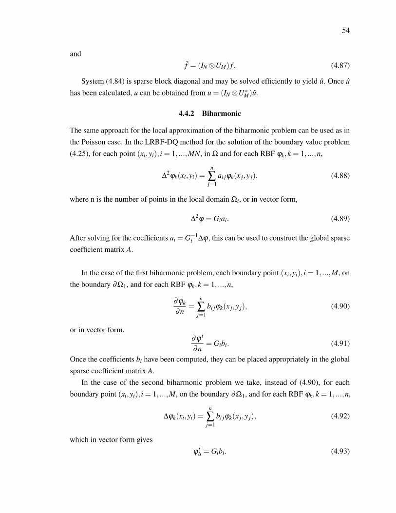
54

andf = (IN⊗UM) f . (4.87)

System (4.84) is sparse block diagonal and may be solved efficiently to yield u. Once u

has been calculated, u can be obtained from u = (IN⊗U∗M)u.

4.4.2 Biharmonic

The same approach for the local approximation of the biharmonic problem can be used as inthe Poisson case. In the LRBF-DQ method for the solution of the boundary value problem(4.25), for each point (xi,yi), i = 1, ...,MN, in Ω and for each RBF ϕk,k = 1, ...,n,

∆2ϕk(xi,yi) =

n

∑j=1

ai jϕk(x j,y j), (4.88)

where n is the number of points in the local domain Ωi, or in vector form,

∆2ϕ = Giai. (4.89)

After solving for the coefficients ai = G−1i ∆ϕ , this can be used to construct the global sparse

coefficient matrix A.

In the case of the first biharmonic problem, each boundary point (xi,yi), i = 1, ...,M, onthe boundary ∂Ω1, and for each RBF ϕk,k = 1, ...,n,

∂ϕk

∂n=

n

∑j=1

bi jϕk(x j,y j), (4.90)

or in vector form,∂ϕ i

∂n= Gibi. (4.91)

Once the coefficients bi have been computed, they can be placed appropriately in the globalsparse coefficient matrix A.

In the case of the second biharmonic problem we take, instead of (4.90), for eachboundary point (xi,yi), i = 1, ...,M, on the boundary ∂Ω1, and for each RBF ϕk,k = 1, ...,n,

∆ϕk(xi,yi) =n

∑j=1

bi jϕk(x j,y j), (4.92)

which in vector form givesϕ

i∆ = Gibi. (4.93)

55

As in the first biharmonic problem, the coefficients bi can be put in the global coefficientmatrix A. In both biharmonic problems, the assembly of all equations for the MN centers(xi,yi), yields an MN×MN system of the form (4.80). Having the same circulant structureas in the Poisson case, the system can be solved using the MDA as explained in the previoussection.

4.4.3 Cauchy Navier

In the LRBF-DQ method for the solution of the boundary value problem (4.45), for eachpoint (xi,yi), i = 1, ...,MN, in Ω and for each RBF ϕk,k = 1, ...,n,

L11ϕk(xi,yi) =n

∑j=1

aikl ϕk(x j,y j), L12ϕk(xi,yi) =

n

∑j=1

bikl ϕk(x j,y j),

L21ϕk(xi,yi) =n

∑j=1

ci jkl ϕk(x j,y j), L22ϕk(xi,yi) =

n

∑j=1

di jkl ϕk(x j,y j),

which in vector form gives for each point (xi,yi),

ϕiL11

= Giai, ϕiL12

= Gibi, ϕiL21

= Gici, ϕiL22

= Gidi. (4.94)

After solving for the coefficients, ai,bi,ci,di, this can be used to construct the global sparse

coefficient matrix A =

(A BC D

)The Dirichlet boundary condition is applied separately for u1 and u2 as in (4.77). TheNeumann boundary condition is applied as follows

T11ϕ(xi,yi) =

[2µ

(1−ν

1−2ν

)∂

∂xnx +µ

∂

∂yny

]ϕ(xi,yi) =

n

∑j=1

ei jϕ(x j,y j),

T12ϕ(xi,yi) =

[2µ

(ν

1−2ν

)∂

∂ynx +µ

∂

∂xny

]ϕ(xi,yi) =

n

∑j=1

fi jϕ(x j,y j),

T21ϕ(xi,yi) =

[µ

∂

∂ynx +2µ

(ν

1−2ν

)∂

∂xny

]ϕ(xi,yi) =

n

∑j=1

gi jϕ(x j,y j),

T22ϕ(xi,yi) =

[µ

∂

∂xnx +2µ

(1−ν

1−2ν

)∂

∂yny

]ϕ(xi,yi) =

n

∑j=1

hi jϕ(x j,y j),

where n is the number of points in the local domain Ωi, or in vector form,

ϕiT11

= Giei, ϕiT12

= Gi fi, ϕiT21

= Gigi, ϕiT22

= Gihi. (4.95)

Once the coefficients ei, fi,gi,hi have been computed, they can be placed appropriately inthe global coefficient matrix A. Assembling all equations for the MN centers (xi,yi), yields

56

a 2MN× 2MN system of the form (4.80). While the matrix A is sparse, it is not blockcirculant. However, a transformation is possible for the local case as explained in section4.2. Once A is transformed to a block circulant matrix, the system can be solved using theMDA as explained in section 4.3.

57

Chapter 5

NUMERICAL RESULTS

In this chapter, numerical results obtained from the Radial Basis Function DifferentialQuadrature method (RBF-DQ) using the Matrix Decomposition Algorithm (MDA) arepresented. This method approximates the particular solution for large scale elliptic partialdifferential equations (PDEs). The normal multiquadric (NMQ) has achieved excellentresults in the RBF literature. Other notable RBFs include the Inverse Multiquadric (IMQ)and Gaussian. The accuracy of the method is dependent upon the selection of the shapeparameter for each of the RBFs. For the global RBF-DQ method, the adjusted Fausshauerestimate will be applied for the selection of the shape parameter. Experiments will alsobe considered using the well known leave-one-out cross validation (LOOCV) method, amethod described in Chapter 2. As the number of collocation points increases, LOOCVbecomes computationally expensive, thus a modification is required. Instead of using theentire set of MN collocation points, LOOCV will be applied to the set of M collocationpoints on a randomly selected concentric circle. This will provide satisfactory results giventhe nature of the point distribution. For the local RBF-DQ method, LOOCV is also used todetermine a suitable shape parameter. Instead of applying LOOCV to each local domain, itcan be applied to only one local domain to calculate the shape parameter, and this value willbe used for all local domains.

Experiments are also conducted using the dimensionless shape parameter, where theproposed value of c = MN/1000 is used, and is compared with the value found usingLOOCV. Several problems with known exact solutions are used to verify the effectivenessof the proposed method including the Poisson, Biharmonic, and Cauchy-Navier equations.While implementing the numerical schemes, an annulus is used for the domain. Thecomputations were carried out using MATLAB on a Macbook Pro laptop with 2.8 GHzIntel Core i7, 16 GB memory, in OS X 10.11.6 for up to M = N = 700 in the global method.For larger sets of collocation points, it was necessary to use a workstation with a largermemory storage of 256GB. Using this workstation, a problem using up to one million points(M = N = 1000) was successfully solved. The local method, however, is able to handle upto one million points without the need of using the larger workstation.

To validate the numerical accuracy, the maximum relative error E is calculated and is

58

defined as

E =||u−uN ||∞,Ω

||u||∞,Ω

, (5.1)

where u and uN denote the exact solution and the approximate solution, respectively.

5.1 Poisson Equation RBF-DQ

Consider the Poisson problem

∆u = 5e2x+y in Ω, (5.2a)

u = e2x+y on ∂Ω1,∂Ω2. (5.2b)

with the domain Ω defined by γ1 = 0.3 and γ2 = 1. The boundary conditions correspond tothe exact solution which is given by u = e2x+y. The profile of the exact solution is shown inFigure 5.1. The profile of the relative error is shown in Figure 5.2. In Figures 5.3-5.5 the

Figure 5.1: Example 1: Profile of the Exact Solution.

maximum relative error E is plotted versus the shape parameter c for M = N = 100 for eachof the MQ, IMQ, and Gaussian RBFs. In these figures, it can be observed that all three RBFsbehave similarly for values up to c = 4. Beyond this value, the accuracy for IMQ begins todetoriate while the accuracy for MQ continues to improve up to c = 5 before detoriating.While the Gaussian RBF displays less stability, the accuracy appears to be fairly steady. Infact, this trend continues through c = 100 as shown in Figure 5.6.

Table 5.1 displays the optimal shape parameter with its corresponding maximum relativeerror for each of the three RBFs. Excellent results are obtained from each of the three tested

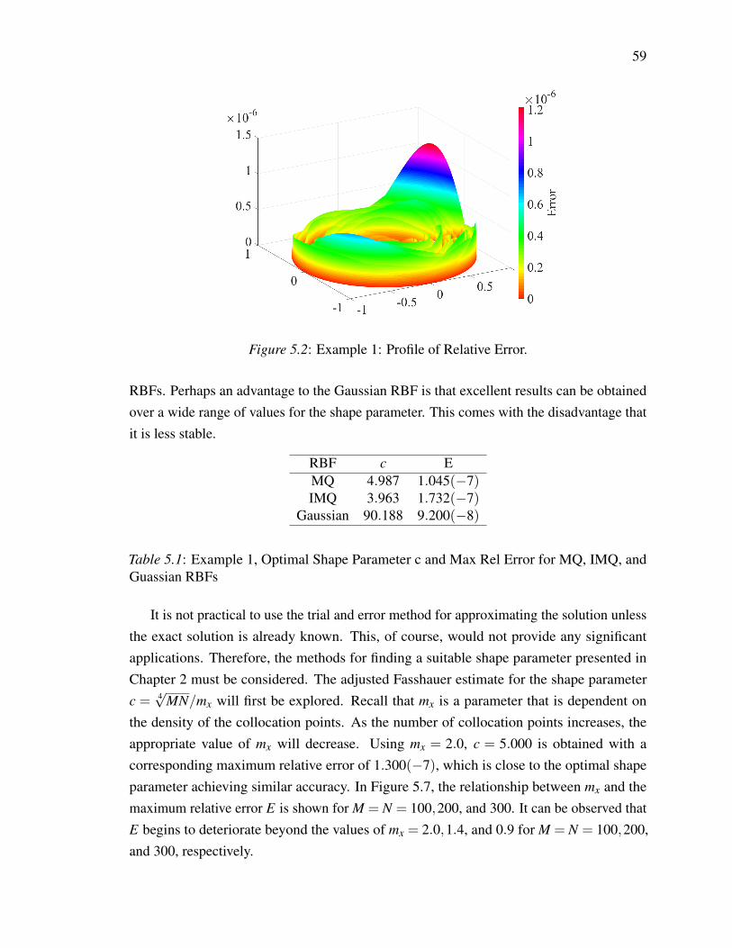
59

Figure 5.2: Example 1: Profile of Relative Error.

RBFs. Perhaps an advantage to the Gaussian RBF is that excellent results can be obtainedover a wide range of values for the shape parameter. This comes with the disadvantage thatit is less stable.

RBF c EMQ 4.987 1.045(−7)IMQ 3.963 1.732(−7)

Gaussian 90.188 9.200(−8)

Table 5.1: Example 1, Optimal Shape Parameter c and Max Rel Error for MQ, IMQ, andGuassian RBFs

It is not practical to use the trial and error method for approximating the solution unlessthe exact solution is already known. This, of course, would not provide any significantapplications. Therefore, the methods for finding a suitable shape parameter presented inChapter 2 must be considered. The adjusted Fasshauer estimate for the shape parameterc = 4√

MN/mx will first be explored. Recall that mx is a parameter that is dependent onthe density of the collocation points. As the number of collocation points increases, theappropriate value of mx will decrease. Using mx = 2.0, c = 5.000 is obtained with acorresponding maximum relative error of 1.300(−7), which is close to the optimal shapeparameter achieving similar accuracy. In Figure 5.7, the relationship between mx and themaximum relative error E is shown for M = N = 100,200, and 300. It can be observed thatE begins to deteriorate beyond the values of mx = 2.0,1.4, and 0.9 for M = N = 100,200,and 300, respectively.

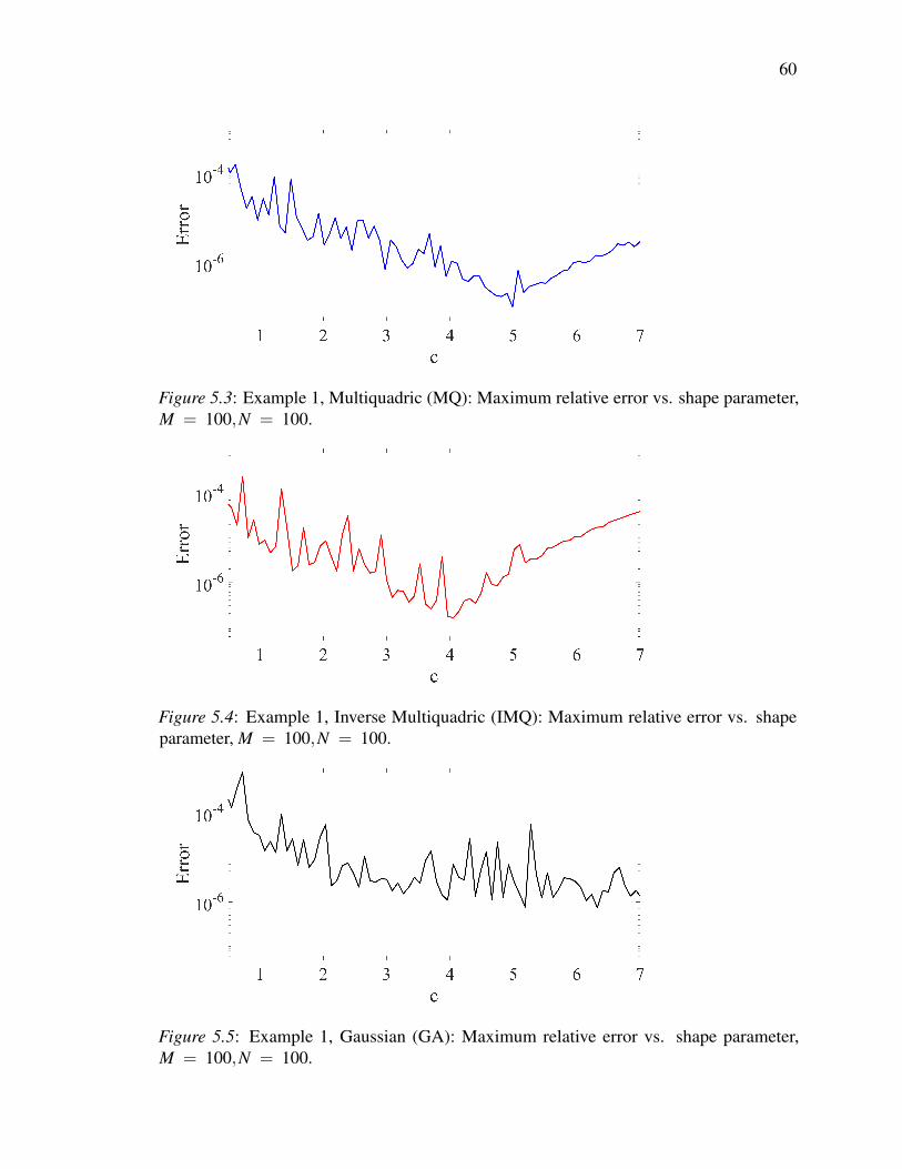
60

Figure 5.3: Example 1, Multiquadric (MQ): Maximum relative error vs. shape parameter,M = 100,N = 100.

Figure 5.4: Example 1, Inverse Multiquadric (IMQ): Maximum relative error vs. shapeparameter, M = 100,N = 100.

Figure 5.5: Example 1, Gaussian (GA): Maximum relative error vs. shape parameter,M = 100,N = 100.

61

Figure 5.6: Example 1, Gaussian (GA): Maximum relative error versus shape parameterwith M = 100,N = 100.

Figure 5.7: Example 1, Poisson Dirichlet problem: Maximum relative error versus mx usingMQ.

Using the above selection procedure, the values of mx have been chosen as shown inTable 5.2 for M = N values up to 700 for the Dirichlet boundary problem (4.1a-4.1c) withthe MQ RBF.

To demonstrate the accuracy up to one million points (M = 1000,N = 1000), Table5.3 shows the results using the workstation with 256 GB memory.

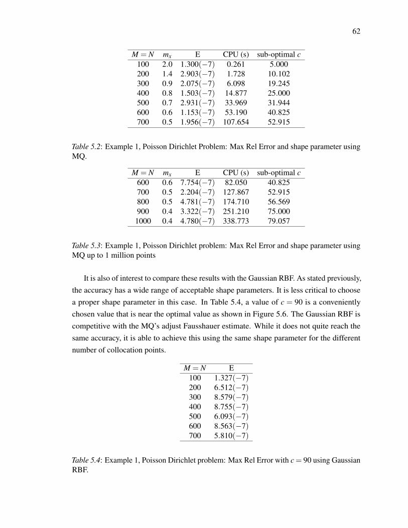
62

M = N mx E CPU (s) sub-optimal c100 2.0 1.300(−7) 0.261 5.000200 1.4 2.903(−7) 1.728 10.102300 0.9 2.075(−7) 6.098 19.245400 0.8 1.503(−7) 14.877 25.000500 0.7 2.931(−7) 33.969 31.944600 0.6 1.153(−7) 53.190 40.825700 0.5 1.956(−7) 107.654 52.915

Table 5.2: Example 1, Poisson Dirichlet Problem: Max Rel Error and shape parameter usingMQ.

M = N mx E CPU (s) sub-optimal c600 0.6 7.754(−7) 82.050 40.825700 0.5 2.204(−7) 127.867 52.915800 0.5 4.781(−7) 174.710 56.569900 0.4 3.322(−7) 251.210 75.000

1000 0.4 4.780(−7) 338.773 79.057

Table 5.3: Example 1, Poisson Dirichlet problem: Max Rel Error and shape parameter usingMQ up to 1 million points

It is also of interest to compare these results with the Gaussian RBF. As stated previously,the accuracy has a wide range of acceptable shape parameters. It is less critical to choosea proper shape parameter in this case. In Table 5.4, a value of c = 90 is a convenientlychosen value that is near the optimal value as shown in Figure 5.6. The Gaussian RBF iscompetitive with the MQ’s adjust Fausshauer estimate. While it does not quite reach thesame accuracy, it is able to achieve this using the same shape parameter for the differentnumber of collocation points.

M = N E100 1.327(−7)200 6.512(−7)300 8.579(−7)400 8.755(−7)500 6.093(−7)600 8.563(−7)700 5.810(−7)

Table 5.4: Example 1, Poisson Dirichlet problem: Max Rel Error with c = 90 using GaussianRBF.

63

Table 5.5 shows results for the Dirichlet/Neumann boundary problem (5.2) replacing(5.2b) with ∂u

∂n = ∇e2x+y ·n on the boundary ∂Ω1 for M = N up to 700 using MQ.

M = N mx E CPU (s) sub-optimal c100 2.0 1.462(−7) 0.263 5.000200 1.4 1.447(−7) 1.730 10.102300 0.9 2.040(−7) 6.075 19.245400 0.8 3.096(−7) 14.970 25.000500 0.7 1.236(−7) 33.989 31.944600 0.6 4.919(−7) 53.988 40.825700 0.5 4.966(−7) 109.273 52.915

Table 5.5: Example 1, Poisson Neumann problem: Max Rel Error and shape parameterusing MQ RBF.

It is also noteworthy to compare the MDA with the full RBF-DQ method in which thefull system (4.1) is solved to fully realize the computational savings. In Table 5.6, the errors,E, and CPU times for the full RBF-DQ method and the corresponding values using theproposed RBF-DQ MDA for a range of collocation points using LOOCV to estimate theoptimal shape parameter is displayed. While LOOCV is a valid and well known method,the most time consuming part in both approaches is the search of a suitable shape parameterusing LOOCV, in which systems are repeatedly solved. Taking advantage of the circulantstructure and the distribution of the collocation points, instead of using all of the points inthe domain, we can take a subset of points. Choose for this subset the points on a randomlyselected concentric circle, and use LOOCV with an initial search interval [0,8] to calculatethe suboptimal shape parameter. This approach is used for both the full RBF-DQ method andthe RBF-DQ MDA method with the MQ RBF. Although the LOOCV is using a minimumamount of required computational time, it can be observed that the full RBF-DQ methodquickly becomes burdened by the obligation of solving the full matrix. Time and memorybecome so large, calculations were not able to be recorded beyond M = N = 120 for the fullRBF-DQ method. This clearly demonstrates the advantage and usefulness that the MDAalgorithm is able to offer large scale problems.

5.2 Biharmonic Equation RBF-DQ

Consider the First Biharmonic problem

∆2u = 25e2x+y in Ω, (5.3a)

u = e2x+y and∂u∂n

= ∇e2x+y ·n on ∂Ω1,∂Ω2, (5.3b)

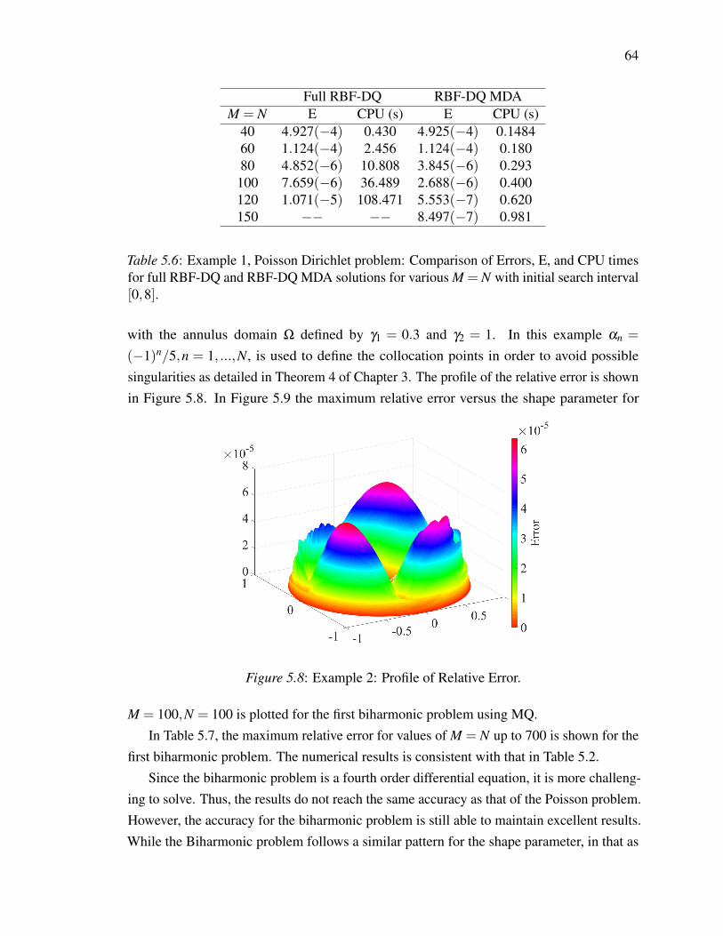
64

Full RBF-DQ RBF-DQ MDAM = N E CPU (s) E CPU (s)

40 4.927(−4) 0.430 4.925(−4) 0.148460 1.124(−4) 2.456 1.124(−4) 0.18080 4.852(−6) 10.808 3.845(−6) 0.293

100 7.659(−6) 36.489 2.688(−6) 0.400120 1.071(−5) 108.471 5.553(−7) 0.620150 −− −− 8.497(−7) 0.981

Table 5.6: Example 1, Poisson Dirichlet problem: Comparison of Errors, E, and CPU timesfor full RBF-DQ and RBF-DQ MDA solutions for various M = N with initial search interval[0,8].

with the annulus domain Ω defined by γ1 = 0.3 and γ2 = 1. In this example αn =

(−1)n/5,n = 1, ...,N, is used to define the collocation points in order to avoid possiblesingularities as detailed in Theorem 4 of Chapter 3. The profile of the relative error is shownin Figure 5.8. In Figure 5.9 the maximum relative error versus the shape parameter for

Figure 5.8: Example 2: Profile of Relative Error.

M = 100,N = 100 is plotted for the first biharmonic problem using MQ.In Table 5.7, the maximum relative error for values of M = N up to 700 is shown for the

first biharmonic problem. The numerical results is consistent with that in Table 5.2.Since the biharmonic problem is a fourth order differential equation, it is more challeng-

ing to solve. Thus, the results do not reach the same accuracy as that of the Poisson problem.However, the accuracy for the biharmonic problem is still able to maintain excellent results.While the Biharmonic problem follows a similar pattern for the shape parameter, in that as

65

Figure 5.9: Example 2, First Biharmonic Problem: Maximum relative error versus shapeparameter with M = 100,N = 100 using MQ.

M = N mx E CPU (s) sub-optimal c100 2.3 2.027(−6) 0.306 4.348200 2.0 8.915(−6) 2.068 7.071300 1.9 1.188(−5) 7.126 9.116400 1.9 1.338(−5) 17.639 10.526500 1.8 2.334(−5) 38.524 12.423600 1.8 1.945(−5) 62.811 13.608700 1.7 2.494(−5) 128.802 15.563

Table 5.7: Example 2, First Biharmonic Problem: Max Rel Error and shape parameter usingMQ.

the number of collocation points increases, the value mx decreases. However, the valueshave a narrower range beginning at mx = 2.3 for M = N = 100 and ending at mx = 1.7 forM = N = 700. This is due to the fourth order problem requiring a lower shape parametervalue to achieve optimal accuracy.

Similar results are found using the Gaussian RBF. Again, the advantage that the Gaussianoffers is that the same shape parameter can be used for any size set of collocation pointsas shown in Table 5.8. For the fourth order problem, a smaller shape parameter is chosen,c = 60.

The same results can be seen when changing the boundary conditions for the biharmonicproblem. Tables (5.9) and (5.10) show results for M =N up to 700 for the second biharmonic

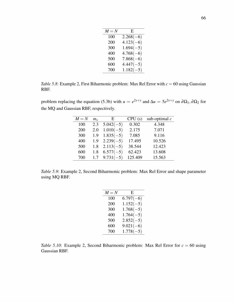
66

M = N E100 2.268(−6)200 4.123(−6)300 1.694(−5)400 4.768(−6)500 7.868(−6)600 4.447(−5)700 1.182(−5)

Table 5.8: Example 2, First Biharmonic problem: Max Rel Error with c = 60 using GaussianRBF.

problem replacing the equation (5.3b) with u = e2x+y and ∆u = 5e2x+y on ∂Ω1,∂Ω2 forthe MQ and Gaussian RBF, respectively.

M = N mx E CPU (s) sub-optimal c100 2.3 5.042(−5) 0.302 4.348200 2.0 1.010(−5) 2.175 7.071300 1.9 1.835(−5) 7.085 9.116400 1.9 2.239(−5) 17.495 10.526500 1.8 2.113(−5) 38.544 12.423600 1.8 6.577(−5) 62.423 13.608700 1.7 9.731(−5) 125.409 15.563

Table 5.9: Example 2, Second Biharmonic problem: Max Rel Error and shape parameterusing MQ RBF.

M = N E100 6.797(−6)200 1.152(−5)300 1.768(−5)400 1.764(−5)500 2.852(−5)600 9.021(−6)700 1.778(−5)

Table 5.10: Example 2, Second Biharmonic problem: Max Rel Error for c = 60 usingGaussian RBF.

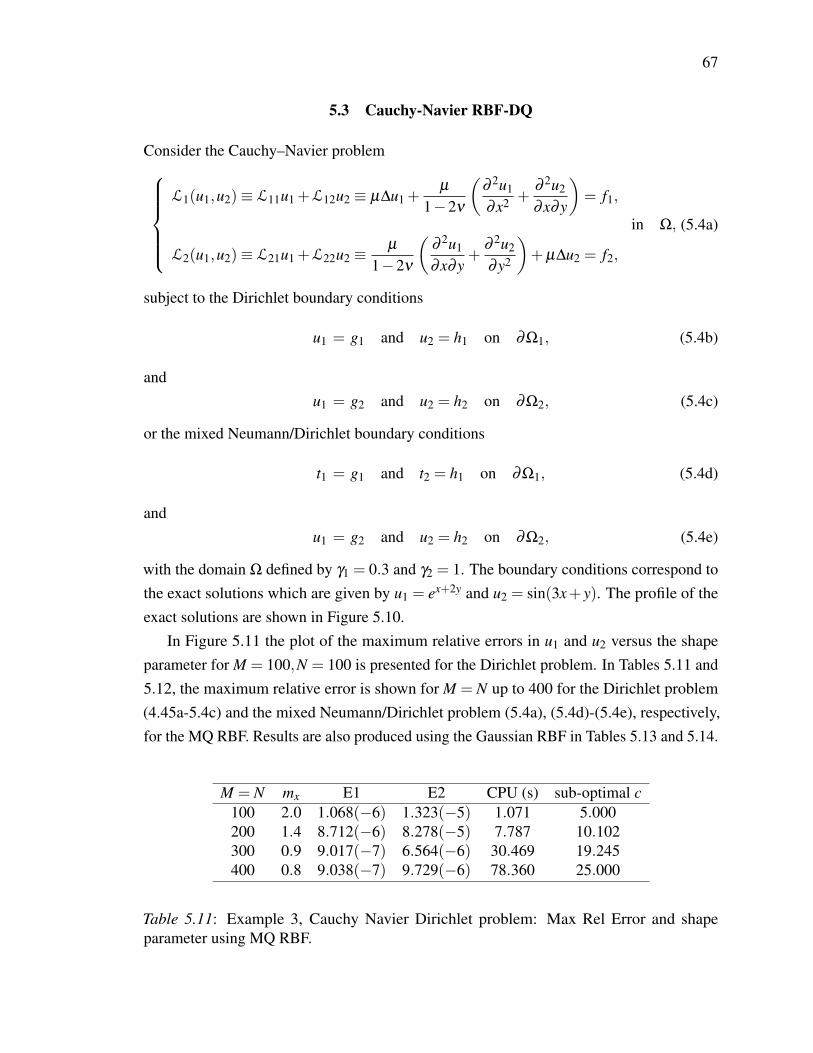
67

5.3 Cauchy-Navier RBF-DQ

Consider the Cauchy–Navier problemL1(u1,u2)≡ L11u1 +L12u2 ≡ µ∆u1 +

µ

1−2ν

(∂ 2u1

∂x2 +∂ 2u2

∂x∂y

)= f1,

in Ω,

L2(u1,u2)≡ L21u1 +L22u2 ≡µ

1−2ν

(∂ 2u1

∂x∂y+

∂ 2u2

∂y2

)+µ∆u2 = f2,

(5.4a)

subject to the Dirichlet boundary conditions

u1 = g1 and u2 = h1 on ∂Ω1, (5.4b)

andu1 = g2 and u2 = h2 on ∂Ω2, (5.4c)

or the mixed Neumann/Dirichlet boundary conditions

t1 = g1 and t2 = h1 on ∂Ω1, (5.4d)

andu1 = g2 and u2 = h2 on ∂Ω2, (5.4e)

with the domain Ω defined by γ1 = 0.3 and γ2 = 1. The boundary conditions correspond tothe exact solutions which are given by u1 = ex+2y and u2 = sin(3x+ y). The profile of theexact solutions are shown in Figure 5.10.

In Figure 5.11 the plot of the maximum relative errors in u1 and u2 versus the shapeparameter for M = 100,N = 100 is presented for the Dirichlet problem. In Tables 5.11 and5.12, the maximum relative error is shown for M = N up to 400 for the Dirichlet problem(4.45a-5.4c) and the mixed Neumann/Dirichlet problem (5.4a), (5.4d)-(5.4e), respectively,for the MQ RBF. Results are also produced using the Gaussian RBF in Tables 5.13 and 5.14.

M = N mx E1 E2 CPU (s) sub-optimal c100 2.0 1.068(−6) 1.323(−5) 1.071 5.000200 1.4 8.712(−6) 8.278(−5) 7.787 10.102300 0.9 9.017(−7) 6.564(−6) 30.469 19.245400 0.8 9.038(−7) 9.729(−6) 78.360 25.000

Table 5.11: Example 3, Cauchy Navier Dirichlet problem: Max Rel Error and shapeparameter using MQ RBF.

68

Figure 5.10: Example 3: Profile of the Exact Solutions, u1 and u2, respectively.

M = N mx E1 E2 CPU (s) sub-optimal c100 2.0 1.929(−7) 1.923(−6) 1.293 5.000200 1.4 1.489(−7) 1.833(−6) 9.435 10.102300 0.9 2.234(−7) 3.217(−6) 36.538 19.245400 0.8 1.246(−7) 1.831(−6) 99.261 25.000

Table 5.12: Example 3, Cauchy Navier Neumann/Dirichlet problem: Max Rel Error andshape parameter using MQ RBF.

M = N E1 E2100 2.351(−7) 2.530(−6)200 2.772(−6) 2.490(−5)300 3.083(−6) 2.149(−5)400 8.088(−7) 1.068(−5)

Table 5.13: Example 3, Cauchy Navier Dirichlet problem: Max Rel Error with c = 90 usingGaussian RBF.

69

Figure 5.11: Example 3, Cauchy Navier Dirichlet problem: Maximum relative error versusshape parameter with M = 100,N = 100 using MQ RBF.

M = N E1 E2100 3.902(−7) 4.358(−6)200 1.890(−6) 1.980(−5)300 3.361(−6) 2.282(−5)400 3.865(−6) 6.451(−5)

Table 5.14: Example 3, Cauchy Navier Neumann/Dirichlet problem: Max Rel Error withc = 90 using Gaussian RBF.

Since the Cauchy-Navier problem is harmonic, the values of mx from the Poissonproblem can be applied to find an appropriate value for the shape parameter for the MQRBF. Having a system of two equations implies that there will be double the collocationpoints being used, which requires more computational time and memory. Therefore, it isonly possible to go up to M = N = 400 using the computer with 16 GB of memory. Yet, thisis still a remarkable accomplishment while achieving a high level of accuracy.

5.4 Poisson Equation LRBF-DQ

Consider the Poisson problem (5.2) with the domain Ω defined by γ1 = 0.3 and γ2 = 1.The boundary conditions correspond to the exact solution which is given by u = e2x+y. Inthe local approach, the leave-one-out cross validation method is a valid tool for finding asuboptimal shape parameter. Because of the circulant nature of the distribution of collocation

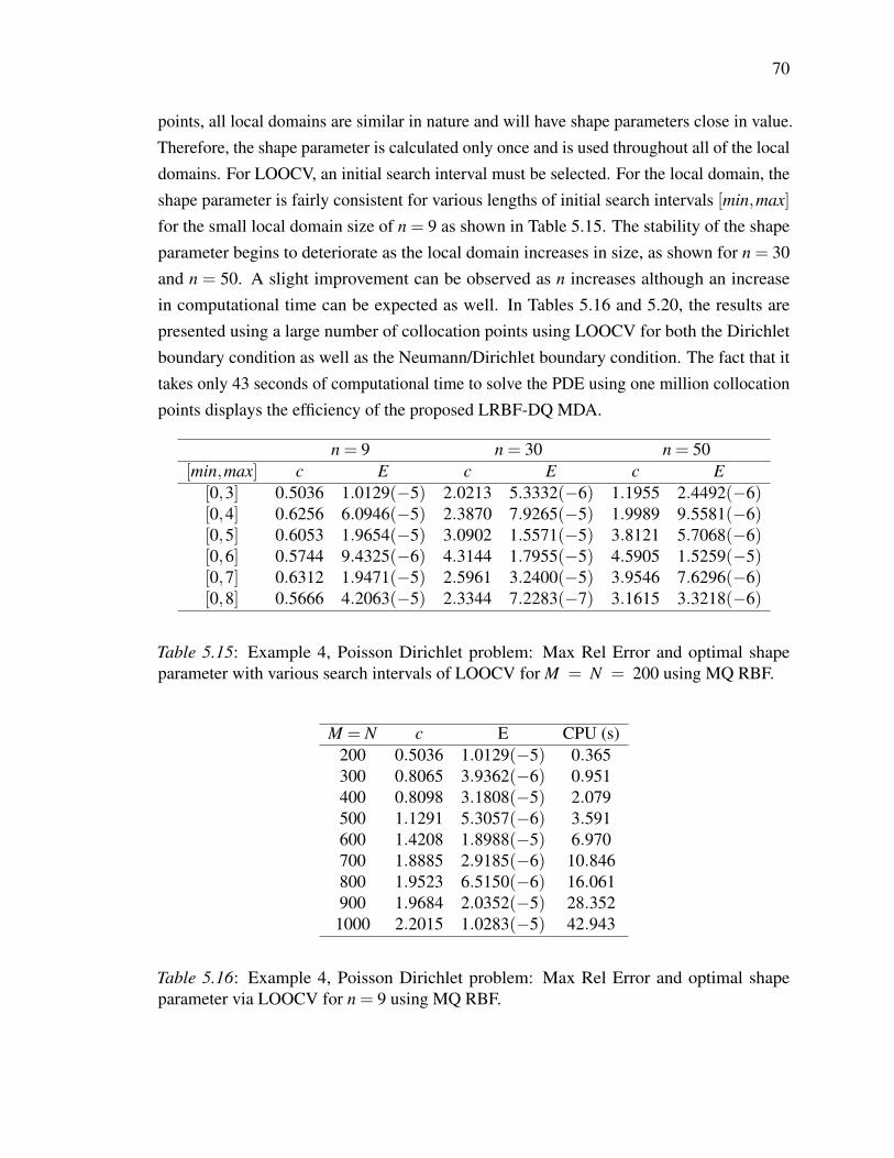
70

points, all local domains are similar in nature and will have shape parameters close in value.Therefore, the shape parameter is calculated only once and is used throughout all of the localdomains. For LOOCV, an initial search interval must be selected. For the local domain, theshape parameter is fairly consistent for various lengths of initial search intervals [min,max]

for the small local domain size of n = 9 as shown in Table 5.15. The stability of the shapeparameter begins to deteriorate as the local domain increases in size, as shown for n = 30and n = 50. A slight improvement can be observed as n increases although an increasein computational time can be expected as well. In Tables 5.16 and 5.20, the results arepresented using a large number of collocation points using LOOCV for both the Dirichletboundary condition as well as the Neumann/Dirichlet boundary condition. The fact that ittakes only 43 seconds of computational time to solve the PDE using one million collocationpoints displays the efficiency of the proposed LRBF-DQ MDA.

n = 9 n = 30 n = 50[min,max] c E c E c E

[0,3] 0.5036 1.0129(−5) 2.0213 5.3332(−6) 1.1955 2.4492(−6)[0,4] 0.6256 6.0946(−5) 2.3870 7.9265(−5) 1.9989 9.5581(−6)[0,5] 0.6053 1.9654(−5) 3.0902 1.5571(−5) 3.8121 5.7068(−6)[0,6] 0.5744 9.4325(−6) 4.3144 1.7955(−5) 4.5905 1.5259(−5)[0,7] 0.6312 1.9471(−5) 2.5961 3.2400(−5) 3.9546 7.6296(−6)[0,8] 0.5666 4.2063(−5) 2.3344 7.2283(−7) 3.1615 3.3218(−6)

Table 5.15: Example 4, Poisson Dirichlet problem: Max Rel Error and optimal shapeparameter with various search intervals of LOOCV for M = N = 200 using MQ RBF.

M = N c E CPU (s)200 0.5036 1.0129(−5) 0.365300 0.8065 3.9362(−6) 0.951400 0.8098 3.1808(−5) 2.079500 1.1291 5.3057(−6) 3.591600 1.4208 1.8988(−5) 6.970700 1.8885 2.9185(−6) 10.846800 1.9523 6.5150(−6) 16.061900 1.9684 2.0352(−5) 28.352

1000 2.2015 1.0283(−5) 42.943

Table 5.16: Example 4, Poisson Dirichlet problem: Max Rel Error and optimal shapeparameter via LOOCV for n = 9 using MQ RBF.

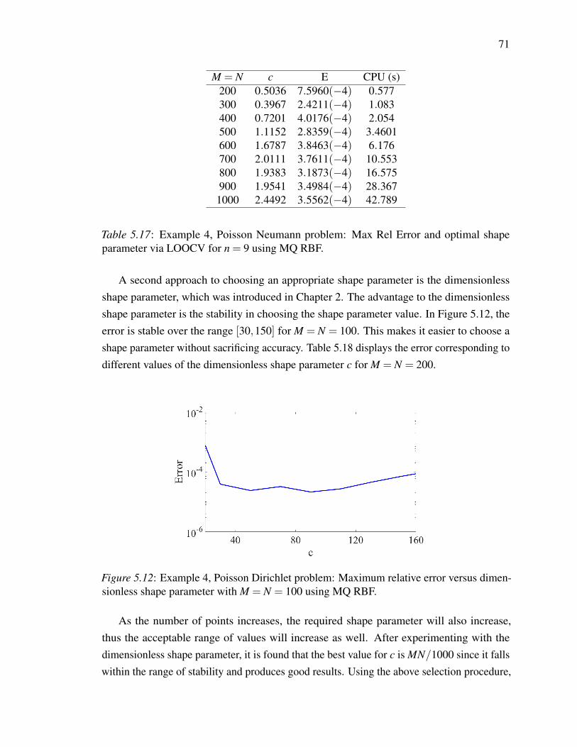
71

M = N c E CPU (s)200 0.5036 7.5960(−4) 0.577300 0.3967 2.4211(−4) 1.083400 0.7201 4.0176(−4) 2.054500 1.1152 2.8359(−4) 3.4601600 1.6787 3.8463(−4) 6.176700 2.0111 3.7611(−4) 10.553800 1.9383 3.1873(−4) 16.575900 1.9541 3.4984(−4) 28.367

1000 2.4492 3.5562(−4) 42.789

Table 5.17: Example 4, Poisson Neumann problem: Max Rel Error and optimal shapeparameter via LOOCV for n = 9 using MQ RBF.

A second approach to choosing an appropriate shape parameter is the dimensionlessshape parameter, which was introduced in Chapter 2. The advantage to the dimensionlessshape parameter is the stability in choosing the shape parameter value. In Figure 5.12, theerror is stable over the range [30,150] for M = N = 100. This makes it easier to choose ashape parameter without sacrificing accuracy. Table 5.18 displays the error corresponding todifferent values of the dimensionless shape parameter c for M = N = 200.

Figure 5.12: Example 4, Poisson Dirichlet problem: Maximum relative error versus dimen-sionless shape parameter with M = N = 100 using MQ RBF.

As the number of points increases, the required shape parameter will also increase,thus the acceptable range of values will increase as well. After experimenting with thedimensionless shape parameter, it is found that the best value for c is MN/1000 since it fallswithin the range of stability and produces good results. Using the above selection procedure,

72

c cr0 E10 0.1881 1.5167(−2)30 0.5643 3.8797(−5)50 0.9404 2.3853(−5)70 1.3166 3.2355(−5)

110 2.0690 2.7129(−5)150 2.8213 7.0490(−5)190 3.5737 1.5479(−4)

Table 5.18: Example 4, Poisson Dirichlet problem M = N = 200: Max Rel Error fordimensionless shape parameter using MQ RBF.

the value of c has been chosen as shown in Table 5.19 for M = N values up to 1000 for theDirichlet boundary problem. The results are consistent with LOOCV without the need ofchoosing an appropriate inital search interval.

M = N c E CPU (s)200 40 1.6939(−5) 0.371300 90 4.9842(−6) 1.003400 160 1.545(−5) 2.144500 250 1.4673(−5) 3.630600 360 3.2208(−6) 6.959700 490 3.3203(−6) 10.949800 640 1.5099(−6) 16.979900 810 2.7664(−6) 28.1011000 1000 6.2346(−5) 41.485

Table 5.19: Example 4, Poisson Dirichlet problem: Max Rel Error with c = MN/1000 usingMQ RBF.

In order to obtain a more accurate RBF approximation, it is necessary to balance thesize of the supporting domain and the sensitivity of the shape parameter. In Table 5.21, themaximum error is calculated with various local domain sizes using the dimensionless shapeparameter. As the number of nodes in the local domain increases, the computational timeincreases and does not have a noteable difference in accuracy with the exception of n = 5.The LRBF-DQ provides accurate approximate solutions even with a small local domain size.For the given distribution of the collocation points, it is only necessary to use nine points inthe local domain to reach satisfactory results.

73

M = N c E CPU (s)200 40 8.3935(−4) 0.611300 90 5.8175(−4) 1.240400 160 5.1726(−4) 2.391500 250 5.3007(−4) 3.967600 360 5.0164(−4) 7.365700 490 4.5828(−4) 11.958800 640 5.0732(−4) 16.976900 810 5.5363(−4) 30.1671000 1000 5.4880(−4) 44.911

Table 5.20: Example 4, Poisson Neumann problem: Max Rel Error with c = MN/1000using MQ RBF.

n E CPU (s) c5 1.2341(−2) 5.5479 1.60629 1.4673(−5) 5.6120 1.886015 6.6101(−5) 5.8642 2.909130 4.4999(−5) 6.2422 4.195640 1.1590(−5) 5.9229 4.816880 6.6619(−6) 6.425 7.0315121 3.1574(−5) 6.554 8.8442

Table 5.21: Example 4, Poisson Dirichlet problem: Influence Domain for M=N=500 usingMQ RBF.

5.5 Biharmonic Equation LRBF-DQ

Consider the Biharmonic problem (5.3) with the domain Ω defined by γ1 = 0.3 and γ2 = 1.In this example, collocation points are defined with αn = (−1)n/5,n = 1, ...,N, to avoidpossible singularities. The boundary conditions correspond to the exact solution, which isgiven by u = e2x+y.The profile of the error versus the shape parameter c for M = N = 80,200,n = 30 is givenin Figure 5.13.

Although there is fluctuation in the curve for M = N = 80, the estimation of a goodshape parameter using LOOCV is fairly stable for various initial search intervals as shownin Tables 5.22 and 5.23 for the first and second biharmonic equation, respectively.

In the case n = 9, the solution is stable in terms of the shape parameter, however theaccuracy does not achieve the same results as that of n = 30. The accuracy does not appearto have a significant improvement with an increase in the size of the local domain for n = 50.

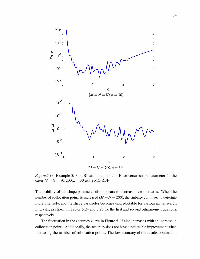
74

[M = N = 80,n = 30]

[M = N = 200,n = 30]

Figure 5.13: Example 5: First Biharmonic problem: Error versus shape parameter for thecases M = N = 80,200,n = 30 using MQ RBF.

The stability of the shape parameter also appears to decrease as n increases. When thenumber of collocation points is increased (M = N = 200), the stability continues to detoriatemore intensely, and the shape parameter becomes unpredictable for various initial searchintervals, as shown in Tables 5.24 and 5.25 for the first and second biharmonic equations,respectively.

The fluctuation in the accuracy curve in Figure 5.13 also increases with an increase incollocation points. Additionally, the accuracy does not have a noticeable improvement whenincreasing the number of collocation points. The low accuracy of the results obtained in

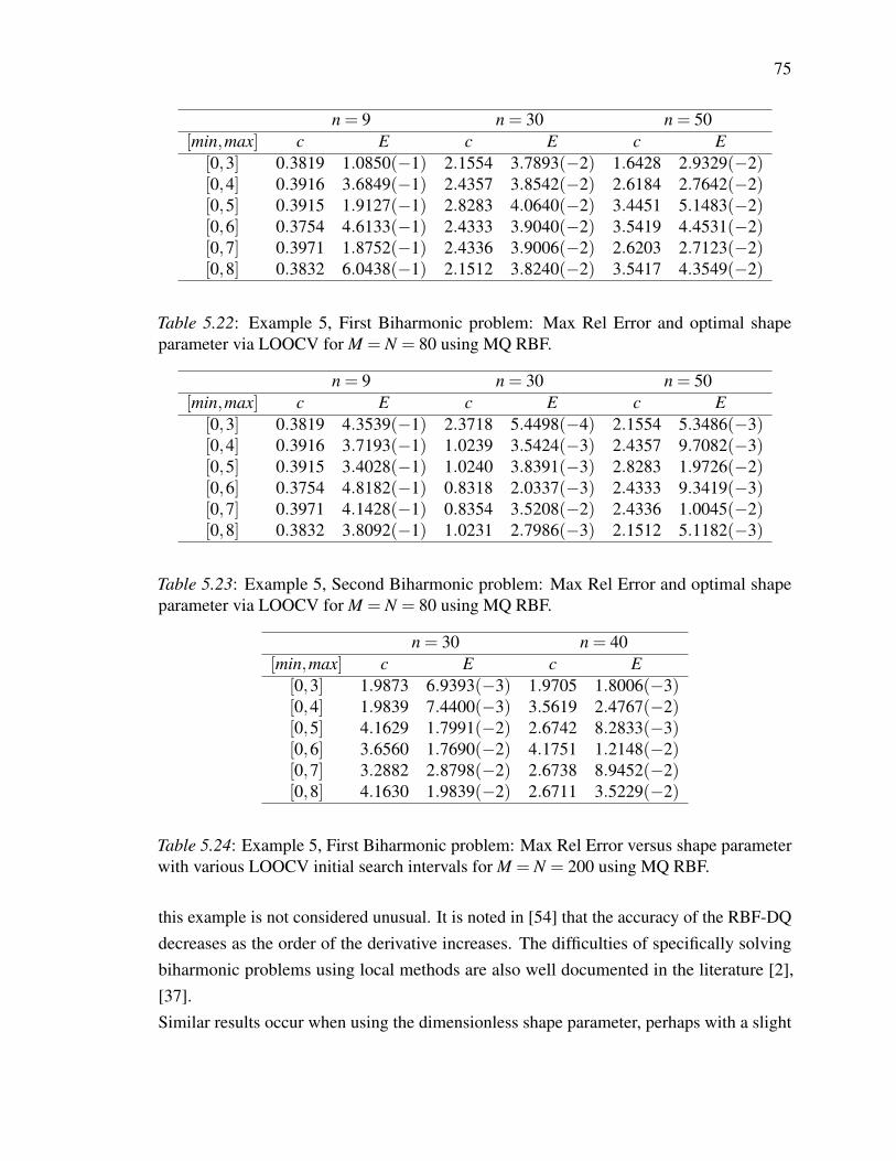
75

n = 9 n = 30 n = 50[min,max] c E c E c E

[0,3] 0.3819 1.0850(−1) 2.1554 3.7893(−2) 1.6428 2.9329(−2)[0,4] 0.3916 3.6849(−1) 2.4357 3.8542(−2) 2.6184 2.7642(−2)[0,5] 0.3915 1.9127(−1) 2.8283 4.0640(−2) 3.4451 5.1483(−2)[0,6] 0.3754 4.6133(−1) 2.4333 3.9040(−2) 3.5419 4.4531(−2)[0,7] 0.3971 1.8752(−1) 2.4336 3.9006(−2) 2.6203 2.7123(−2)[0,8] 0.3832 6.0438(−1) 2.1512 3.8240(−2) 3.5417 4.3549(−2)

Table 5.22: Example 5, First Biharmonic problem: Max Rel Error and optimal shapeparameter via LOOCV for M = N = 80 using MQ RBF.

n = 9 n = 30 n = 50[min,max] c E c E c E

[0,3] 0.3819 4.3539(−1) 2.3718 5.4498(−4) 2.1554 5.3486(−3)[0,4] 0.3916 3.7193(−1) 1.0239 3.5424(−3) 2.4357 9.7082(−3)[0,5] 0.3915 3.4028(−1) 1.0240 3.8391(−3) 2.8283 1.9726(−2)[0,6] 0.3754 4.8182(−1) 0.8318 2.0337(−3) 2.4333 9.3419(−3)[0,7] 0.3971 4.1428(−1) 0.8354 3.5208(−2) 2.4336 1.0045(−2)[0,8] 0.3832 3.8092(−1) 1.0231 2.7986(−3) 2.1512 5.1182(−3)

Table 5.23: Example 5, Second Biharmonic problem: Max Rel Error and optimal shapeparameter via LOOCV for M = N = 80 using MQ RBF.

n = 30 n = 40[min,max] c E c E

[0,3] 1.9873 6.9393(−3) 1.9705 1.8006(−3)[0,4] 1.9839 7.4400(−3) 3.5619 2.4767(−2)[0,5] 4.1629 1.7991(−2) 2.6742 8.2833(−3)[0,6] 3.6560 1.7690(−2) 4.1751 1.2148(−2)[0,7] 3.2882 2.8798(−2) 2.6738 8.9452(−2)[0,8] 4.1630 1.9839(−2) 2.6711 3.5229(−2)

Table 5.24: Example 5, First Biharmonic problem: Max Rel Error versus shape parameterwith various LOOCV initial search intervals for M = N = 200 using MQ RBF.

this example is not considered unusual. It is noted in [54] that the accuracy of the RBF-DQdecreases as the order of the derivative increases. The difficulties of specifically solvingbiharmonic problems using local methods are also well documented in the literature [2],[37].Similar results occur when using the dimensionless shape parameter, perhaps with a slight

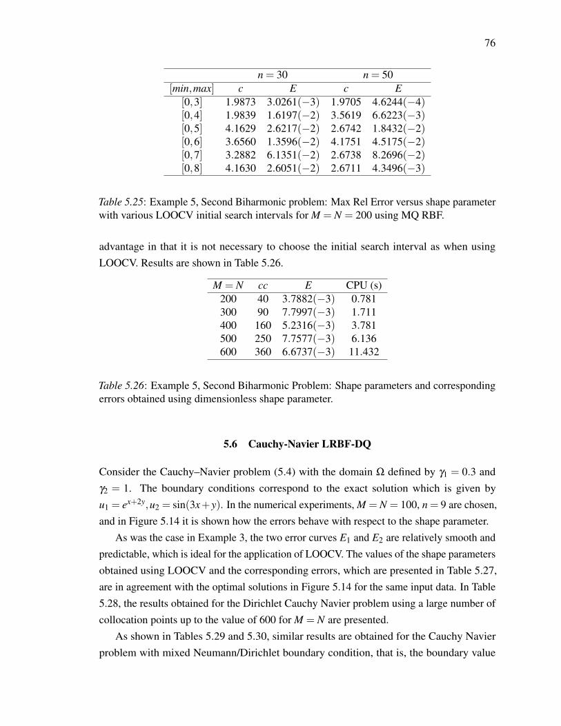
76

n = 30 n = 50[min,max] c E c E

[0,3] 1.9873 3.0261(−3) 1.9705 4.6244(−4)[0,4] 1.9839 1.6197(−2) 3.5619 6.6223(−3)[0,5] 4.1629 2.6217(−2) 2.6742 1.8432(−2)[0,6] 3.6560 1.3596(−2) 4.1751 4.5175(−2)[0,7] 3.2882 6.1351(−2) 2.6738 8.2696(−2)[0,8] 4.1630 2.6051(−2) 2.6711 4.3496(−3)

Table 5.25: Example 5, Second Biharmonic problem: Max Rel Error versus shape parameterwith various LOOCV initial search intervals for M = N = 200 using MQ RBF.

advantage in that it is not necessary to choose the initial search interval as when usingLOOCV. Results are shown in Table 5.26.

M = N cc E CPU (s)200 40 3.7882(−3) 0.781300 90 7.7997(−3) 1.711400 160 5.2316(−3) 3.781500 250 7.7577(−3) 6.136600 360 6.6737(−3) 11.432

Table 5.26: Example 5, Second Biharmonic Problem: Shape parameters and correspondingerrors obtained using dimensionless shape parameter.

5.6 Cauchy-Navier LRBF-DQ

Consider the Cauchy–Navier problem (5.4) with the domain Ω defined by γ1 = 0.3 andγ2 = 1. The boundary conditions correspond to the exact solution which is given byu1 = ex+2y,u2 = sin(3x+y). In the numerical experiments, M = N = 100, n = 9 are chosen,and in Figure 5.14 it is shown how the errors behave with respect to the shape parameter.

As was the case in Example 3, the two error curves E1 and E2 are relatively smooth andpredictable, which is ideal for the application of LOOCV. The values of the shape parametersobtained using LOOCV and the corresponding errors, which are presented in Table 5.27,are in agreement with the optimal solutions in Figure 5.14 for the same input data. In Table5.28, the results obtained for the Dirichlet Cauchy Navier problem using a large number ofcollocation points up to the value of 600 for M = N are presented.

As shown in Tables 5.29 and 5.30, similar results are obtained for the Cauchy Navierproblem with mixed Neumann/Dirichlet boundary condition, that is, the boundary value

77

Figure 5.14: Example 6: Cauchy Navier problem. Maximum relative error versus shapeparameter for M = N = 100,n = 9 using MQ RBF.

[min,max] c E1 E2[0,3] 0.556 2.005(−4) 1.343(−3)[0,4] 0.563 2.422(−4) 1.394(−3)[0,5] 0.611 1.917(−4) 1.283(−3)[0,6] 0.612 2.982(−4) 2.332(−3)[0,7] 0.616 2.020(−4) 1.325(−3)[0,8] 0.559 2.255(−4) 1.402(−3)

Table 5.27: Example 6, Cauchy Navier Dirichlet problem: Shape parameters and corre-sponding errors obtained with various search intervals of LOOCV; M = N = 100, n = 9using MQ RBF.

M = N c E1 E2 CPU (s)200 1.130 4.636(−4) 3.298(−3) 1.729300 1.706 9.842(−5) 1.049(−3) 4.836400 2.275 1.416(−4) 5.752(−4) 12.322500 2.842 1.888(−4) 1.080(−3) 25.185600 2.796 4.275(−4) 1.804(−3) 50.760

Table 5.28: Example 6, Cauchy Navier Dirichlet problem: Shape parameters and corre-sponding errors obtained using LOOCV with local domain size n = 9 using MQ RBF.

78

problem consisting of (5.4d)-(5.4e).

[min,max] c E1 E2[0,3] 0.556 1.002(−3) 4.115(−3)[0,4] 0.563 1.049(−3) 4.092(−3)[0,5] 0.611 9.928(−4) 4.066(−3)[0,6] 0.612 9.567(−4) 6.526(−3)[0,7] 0.616 1.015(−3) 4.067(−3)[0,8] 0.559 1.030(−3) 4.155(−3)

Table 5.29: Example 6, Cauchy Navier Neumann problem: Shape parameters and corre-sponding errors obtained using various search intervals of LOOCV; M = N = 100,n = 9using MQ RBF.

M = N c E1 E2 CPU (s)200 1.130 3.827(−3) 4.433(−2) 1.885300 1.706 2.472(−4) 2.604(−3) 4.890400 2.275 4.008(−4) 1.933(−3) 9.839500 2.842 5.131(−4) 3.650(−3) 23.529600 2.796 6.442(−4) 3.126(−3) 52.138

Table 5.30: Example 6, Cauchy Navier Neumann problem: Shape parameters and corre-sponding errors obtained using dimensionless shape parameter using MQ RBF.

It is worth noting that a problem consisting of 360,000 collocation points can be solvedin only 50 seconds using a computer with 16 GB of memory space, which demonstrates theefficiency of the proposed algorithm.

79

Chapter 6

CONCLUSIONS AND FUTURE WORKS

6.1 Conclusions

This dissertation developed a new numerical algorithm to solve various types of large scalepartial differential equations. Both a global and local scheme was used for the radial basisfunction differential quadrature method combined with a matrix decomposition algorithm.

The global method is simple, efficient, and accurate in solving these large scale problemsquickly and efficiently. In particular, the global method has been applied to PDEs with up toone million collocation points. The method, due to the nature of RBFs, can easily extendto problems in high-dimensional spaces. The matrix decomposition algorithm developedin this paper requires that the right hand side of the equation be circulant. For the Poissonand Biharmonic problems, this requirement is certainly satisfied. For the Cauchy Navierproblem, however, this is not the case. To overcome this obstacle, the right hand side ofthe differential equation is able to be transformed so that it becomes circulant. Once thetransformation has been completed, the proposed procedure can be continued. The globalmethod has the capability of solving problems up to half a million points before memorybecomes an issue on a laptop using 16 GB of memory. Even so, the global method was usedto solve up to a million points using a workstation with 256 GB of memory.

To overcome the problem of memory as the number of collocation points become large, alocal method has been developed for the RBF Differential Quadrature Matrix DecompositionAlgorithm. Instead of a large dense matrix, as in the global RBF-DQ, the local methodcreates a sparse matrix, which makes it more efficient to solve. Moreover, this sparse matrixis also block circulant allowing the implementation of the matrix decomposition algorithm.In the sense of the Cauchy Navier problem, although this block circulant structure is notpresent, a transformation can again be applied to create the block circulant structure. Specificexamples in this paper have demonstrated that the local method has the ability of solvingproblems with up to a million points in about one minute using a computer with memoryspace of only 16GB.

For the local method, the leave-one-out cross validation method (LOOCV) is effective incalculating a good shape parameter. It was only necessary to calculate the shape parameterfor one local domain and to apply this value for all other local domains due to the circulant

80

structure, which creates similar patterns in each local domain. While LOOCV is not practicalfor the global method due to the large size of the matrix, the adjusted Fasshauer estimatewas employed to calculate an appropriate suboptimal shape parameter. It was observed thatthis value is dependent on the density of the collocation points. As the number of collocationpoints increased, the shape parameter should increase as well, which is controlled by thedecreasing value mx. This Fasshauer estimate works well for solving large scale problemsand does not require significant computational time.

This paper primarliy focused on the normalized multiquadric method for the radial basisfunction. While there are many RBFs that can be used to achieve accurate results, the MQ isthe most commonly used RBF and has consistently produced excellent results. Furthermore,the normalized MQ is stable with regard to the shape parameter meaning that accurateresults can be achieved over a large range of values making it less critical in choosing theshape parameter. Similar results were also achieved using the inverse multiquadric and theGaussian RBF.

While the accuracy of the local method does not achieve the same level of accuracy ofthe global scheme, excellent results are still achieved and provides a significant reductionin the required time and memory. It is worthy to note that the biharmonic problem haslimitations on the accuracy, especially for a local domain size of nine. Better results areachieved when increasing the number of collocation points in the local domain, but thiscomes with the expense of the shape parameter becoming less stable in terms of the searchinterval. This difficulty is not unusual and has been documented in the RBF literature.

It is apparent that meshless methods using local schemes can compete with traditionalnumerical methods for solving large scale PDEs, such as the finite element, finite difference,or finite volume methods. Due to the collocation approach, no numerical integration isrequired. In this dissertation, the numerical results were calculated using a circular domain,more specifically an annulus. This method can extend to other domain types as wellas irregular domains using a conformal mapping procedure. Furthermore, the proposedmethods can be easily extended to solving three-dimensional problems. This is indeed whereits strengths may lie. As such, the approach offers the prospects of an efficient algorithmfor solving more challenging problems in science and engineering. While this work hasnot completely validated the method, the results obtained along with the given analysisdoes provide strong evidence to the utility of the approach and supports the belief that thesemethods developed have a substantial future in solving a wide range of difficult problemsthat occur in the natural sciences and engineering.

81

6.2 Future Works

In this dissertation, the radial basis function differential quadrature method was combinedwith a modified matrix decomposition algorithm that takes advantage of the right hand sideof the equation being block circulant. Both the global and local methods can be used forsolving large scale problems efficiently. As with all new methods, thorough theoreticalanalysis remains to be done, as does the possible extension of the methods to other types ofpartial differential equations. The following topics are of particular interest:

• An MDA method has already been applied to three dimensional problems in [30].The matrix decomposition algorithm employed in the RBF-DQ method suggests thatthis method can be effective for the solution of three dimensional problems as well.

• This study limited the domain to that of an annulus. It is of interest to test theproposed method for a variety of domains using a conformal mapping so that themethod becomes appropriate for irregular domains [22].

• Many engineering problems and other physical phenomena are mostly modeled bynonlinear PDEs. The RBF-DQ method can be applied to nonlinear PDEs. The resultsin this paper suggests that the MDA can also be appropriate for these nonlinear PDEsfor large scale problems.

82

BIBLIOGRAPHY

[1] R. Bellman, B. G. Kashef, and J. Casti. Differential quadrature: a technique for the rapidsolution of nonlinear partial differential equations. J. Comput. Phys., 10, 40-52, 1972.

[2] M. Ben-Artzi, I. Chorev, J. P. Croisille, and D. Fishelov. A compact difference scheme for thebiharmonic equation in planar irregular domains. SIAM J. Numer. Anal., 47:3087-3108, 2009.

[3] B. Bialecki, G. Fairweather, and A. Karageorghis. Matrix decomposition algorithms for ellipticboundary value problems: A survey. Numer. Algorithms, 56,253-295, 2011.

[4] M.D. Buhmann. Radial Basis Functions, Theory and Implementations. Cambridge UniversityPress, 2003.

[5] Y. L. Chan, L. H. Shen, C. T. Wu, and D. L. Young. Interpolation techniques for scattered databy local radial basis function differential quadrature method. Int. J. Comput. Methods, 10:02,2013.

[6] Y. L. Chan, L. H. Shen, C. T. Wu, and D. L. Young. A novel upwind-based local radial basisfunction differential quadrature method for convection-dominated flows. Computers and Fluids,89:157-166, 2014.

[7] C.S. Chen, C.M Fan, and P.H. Wen. The method of particular solutions for solving ellipticproblems with variable coefficients. The International Journal for Numerical Methods inBiomedical Engineering, 8:545–559, 2011.

[8] C.S. Chen, C.M Fan, and P.H. Wen. The method of particular solutions for solving certain partialdifferential equations. Numerical Methods for Partial Differential Equations, 28:506–522,2012. doi: 10.1002/num.20631.

[9] C. S. Chen, M. A. Golberg, M. Ganesh, and A. H. D. Cheng. Multilevel compact radial functionsbased computational schemes for some elliptic problems. Computers and Mathematics withApplication, 43:359–378, 2002.

[10] C. S. Chen, Y. C. Hon, and R. A. Schaback. Scientific computing with radial basis functions.Tech. Rep., Department of Mathematics, University of Southern Misissippi, Hattiesburg, MS39406, USA, preprint, 2005.

[11] W. Chen, Z. Fu, and C.S. Chen. Recent advances in Radial basis Function Collocation Methods.Springer, 2013.

[12] C.S. Chen, A. Karageorghis, O. Macchion. A Kansa-Radial Basis Function Method for EllipticBoundary Value Problems in Annular Domains. SIAM J. Sci. Comput., 65:1240-1269, 2015.

[13] P. J. Davis. Circulant Matrices, Second edition. AMS Chelsea Publishing, Providence, RhodeIsland, 1994.

83

[14] H. Ding, C. Shu, K. S. Yeo, and Z. L. Lu. Simulation of natural convection in eccentric annulibetween a square outer cylinder and a circular inner cylinder using local MQ-DQ method.Numerical Heat Transfer, Part A, 47:291-313, 2005.

[15] G. E. Fasshauer and J. G. Zhang. On choosing optimal shape parameters for RBF approximation.Numer. Algorithms, 45, 345-368, 2007.

[16] G. Fasshauer. Solving partial differential equations by collocation with radial basis functions.Proceedings of Chamonix pp 1-6, 1996.

[17] G. Fasshauer. Meshfree Application Method with Matlab. Interdisciplinary MathematicalSciences, 2007.

[18] G. Fornberg, B.and Wright. Stable computation of multiquadric interpolants for all values ofthe shape parameter. CoComput. Math. Appl.:853-867, 2004.

[19] R. Franke. Scattered data interpolation: Tests of some method. Mathematics of Computation,38:181-200, 1982.

[20] R. L. Hardy. Multiquadric equations of topography and other irrgular surfaces. Journal ofGeophysical Research, 76:1905-1915, 1971.

[21] F. Hartmann. Elastostatics, Progress in Boundary Element Methods Vol. 1 (C. A. Brebbia, ed.).Pentech Press, London, 1981, pp. 84–167.

[22] A. R. H. Heryudono and T. A. Driscoll. Radial basis function interpolation on irregular domainthrough conformal transplantation. J. Sci. Comput., 44, 286-300, 2010.

[23] L. Homayoon, M. J. Abadini, and S. M. R. Hashemi. RBF-DQ solution for shallow waterequations. J. Waterway, Port, Coastal, Ocen Eng., 139:45-60, 2013.

[24] Y. C. Hon, R. Schaback, X. Zhou. An adaptive greedy algorithm for solving large rbf collocationproblems. Numerical Algorithms, 32(1):13-25, 2003.

[25] C. S. Huang, Cheng-Feng Lee, and A. H. D. Cheng. Error estimate, optimal shape factor,and high precision computation of multiquadric collocation method. Eng. Analy. BoundaryElements, 31(7):614-623, 2007.

[26] E.J. Kansa. Multiquadrics - a scattered data approximation scheme with applications tocomputational fluid dynamics - I. Comput. Math. Applic., 19(8/9):127–145, 1990.

[27] E.J. Kansa. Multiquadrics - a scattered data approximation scheme with applications tocomputational fluid dynamics - II. Comput. Math. Applic., 19(8/9):147–161, 1990.

[28] A. Karageorghis, The method of fundamental solutions for elliptic problems in circular domainswith mixed boundary conditions. Numer. Algorithms, 68:185-211, 2015.

[29] A. Karageorghis, C. S. Chen, and X-Y. Liu, Kansa-RBF algorithms for elliptic problems inaxisymmetric domains. SIAM J. Sci. Comput., 38, A435-A470, 2016.

[30] A. Karageorghis, C. S. Chen, and Y.-S. Smyrlis, A matrix decomposition RBF algorithm:approximation of functions and their derivatives. Appl. Numer. Math., 57:304-319, 2007.

84

[31] A. Karageorghis, C. S. Chen, and Y.-S. Smyrlis, Matrix decomposition RBF algorithm forsolving 3D elliptic problems. Eng. Anal. Bound. Elem., 33:1368-1373, 2009.

[32] A. Korkmaz and I. Dag, Solitary wave simulations of complex modified Korteweg-de Vriesequation using differential quadrature method. Comput. Phys. Commun., 180:1516-1523, 2009.

[33] A. Krowiak, Hermite type radial basis function-based differential quadrature method for higherorder equations. Appl. Math. Model, 40, 2421-2430, 2016.

[34] E. Larsson and B. Fornberg. A numerical study of some radial basis function based solutionmethods for elliptic PDEs. Comput. math. Appl., 46:891-902, 2003.

[35] C. K. Lee, X. Liu, and S. C. Fan, Local multiquadric approximation for solving boundary valueproblems. Comput. Mech., 30:396-409, 2003.

[36] X. Li and Chen C. S. A mesh-free method using hyperinterpolation and fast fourier transformfor solving differential equation. Eng. Anal. Boundary Elements,28,1253-1260, 2004.

[37] M Li, G. Amazzar, A. Naji, and C. S. Chen, Solving biharmonic equations using the localizedmethod of approximate particular solutions. Int. J. Comput. Math., 91:1790-1801, 2014.

[38] N. A. Libre, A. Emdadi, E. J. Kansa, M. Rahimian, and M. Shekarchi. A stabilized rbfcollocation scheme for neumann type boundary value problems. Computer Modeling inEngineering and Science, 24:61-80,2008.

[39] X. Y. Liu, A. Karageorghis, and C. S. Chen, A Kansa-radial basis function method for ellipticboundary value problems in annular domains. J. Sci. Comput., 65:1240-1269, 2015.

[40] N. Mai-Duy, T. Tran-Cong. Mesh-free radial basis function network methods with domaindecomposition for approximation of functions and numerical solution of poisson’s equation.Eng. Anal. Boundary Elements, 2002, 26:133-156.

[41] The MathWorks, Inc., 3 Apple Hill Dr., Natick, MA, Matlab.

[42] C. A. Micchelli. Interpolation of scattered data: distance matrices and conditionally positivedefinite function. Constr. Approx., 11-22, 1986.

[43] K W Morton and D F Mayers. Numerical Solution of PDEs, an Introduction. CambridgeUniversity Press, 2005.

[44] J N Reddy. An Introduction to the Finite Element Method. McGraw-Hill, Inc., 2006.

[45] S. Rippa. An algorithm for selecting a good value for the parameter c in radial basis functioninterpolation. Advances in Computational Mathematics, 11:193–210, 1999.

[46] R. Schaback, L. Ling. Stable and convergent unsymmetric meshless collocation methods. SIAMJournal on Numerical Analysis, 46:1097-1115, 2008.

[47] I. J. Schoenberg. Metric spaces and completely monotone functions. Annals of Mathematics,39:811-841, 1938.

[48] L. H. Shen, K. H. Tseng, and D. L. Young. Evaluation of multi-order derivatives by local radialbasis function differential quadrature method. J. Mech., 29:67-78, 2013.

85

[49] C. Shu, Y. T. Chew. Fourier expansion-based differential quadrature and its application toHelmholtz eigenvalue problems. Commun. in Numerical Methods, 13:643-653, 1997.

[50] C. Shu, H. Ding, and K. S. Yeo, Local radial basis function-based differential quadraturemethod and its application to solve two-dimensional incompressible navier-stokes equations.Comput. Methods Appl. Mech. Engrg, 192:941-954, 2003).

[51] C. Shu, B. E. Richards. Application of generalised differential quadrature to solve two-dimension incompressible Navier-Stokes equations. Int. J. Numer Methods Fluids, 15:791-798,1992.

[52] C. Shu and Y. L. Wu, Integrated radial basis functions-based differential quadrature methodand its performance. Int. J. Numer. Meth. Fluids, 53:969-984, 2007.

[53] R. Vertnik and B. Sarler. Meshless local radial basis function collocation method for convective-diffusive solid-liquid phase change problems. International Journal of Numerical Methods forEhater and Fluid Flow, 16:617-640, 2006.

[54] Y. L. Wu and C. Shu. Development of RBF-DQ method for derivative approximation and itsapplication to simulate natural convection in concentric annuli. Comput. Mech. 29:477-485,2002.

[55] J. Yang, X. Liu, and P.H. Wen. The local kansa’s method for solving berger equation. EngEng.Anal. Boundary Elements,16-22, 2015.

[56] G. Yao, J. Kolibal, and C. S. Chen. A localized approach for the method of approximateparticular solutions. Comput. Math. Appl., 61(9):2376–2387, May 2011.

[57] G. Yao. Local radial basis function methods for solving partial differential equations. PhDthesis, University of Southern Mississippi, 2010.

[58] X. Zhang, K. Z. Song, M. W. Lu, and X. Liu. Meshless methods based on collocation withradial basis functions. Computational Mechanics, 26:333-343,2000.

[59] X. Zhang, H. Zhu, and L. Kuo. A comparison study of the LMAPS method and the LDQmethod for time-dependent problems. Eng. Anal Boundary Elements, 11:1408-1415, 2013.