Embed Size (px)
Citation preview

Adaptive Quadrature
Two adaptive integration procedures from Gander and Gautschi [2000] for Excel - VBA
adaptsim() Adaptive Lobatto Quadratureadaptlob() Adaptive Simpson Quadrature
Reference
Gander, W. and W. Gautschi [2000] Adaptive Quadrature - Revisited, BIT Vol. 40, No. 1, pp. 84--101.
freely available as "Technical Report 306" (August 1998) from the Eidgenössische Technische Hochschule (ETH) Zürichftp://ftp.inf.ethz.ch/pub/publications/tech-reports/3xx/306.ps.gz
Two adaptive integration procedures from Gander and Gautschi [2000] for Excel - VBA
Gander, W. and W. Gautschi [2000] Adaptive Quadrature - Revisited, BIT Vol. 40, No. 1, pp. 84--101.
freely available as "Technical Report 306" (August 1998) from the Eidgenössische Technische Hochschule (ETH) Zürich
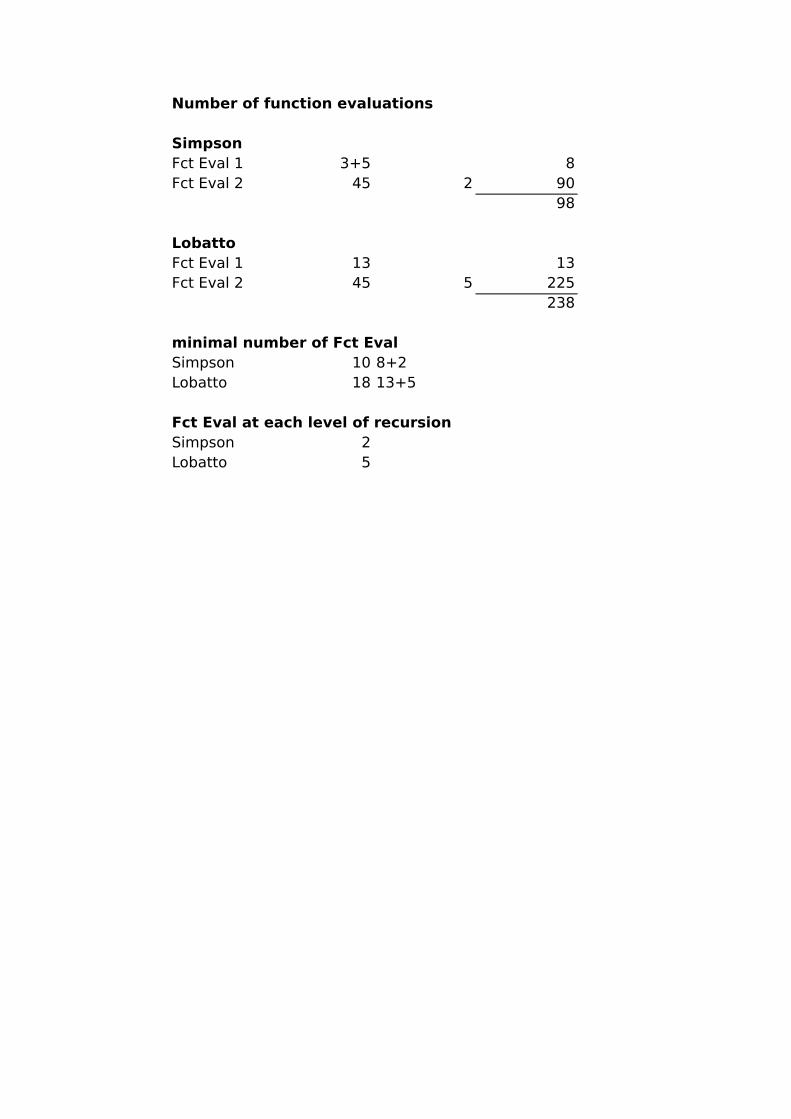
Number of function evaluations
SimpsonFct Eval 1 3+5 8Fct Eval 2 45 2 90
98
LobattoFct Eval 1 13 13Fct Eval 2 45 5 225
238
minimal number of Fct EvalSimpson 10 8+2Lobatto 18 13+5
Fct Eval at each level of recursionSimpson 2Lobatto 5


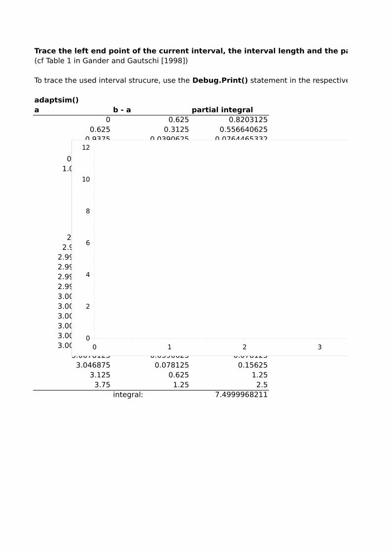
Trace the left end point of the current interval, the interval length and the partial integral(cf Table 1 in Gander and Gautschi [1998])
adaptsim()a b - a partial integral
0 0.625 0.82031250.625 0.3125 0.556640625
0.9375 0.0390625 0.07644653320.9765625 0.01953125 3.88E-02
0.99609375 0.009765625 0.01950560681.005859375 0.009765625 1.94E-02
1.015625 0.078125 0.15197753911.09375 0.15625 0.2856445313
1.25 1.25 1.406252.5 0.3125 0.107421875
2.8125 0.15625 0.01708984382.96875 0.01953125 4.20E-04
2.98828125 0.009765625 6.68E-052.998046875 0.0012207031 1.64E-06
2.9992675781 0.0006103516 2.61E-072.9998779297 7.63E-05 6.40E-092.9999542236 3.81E-05 1.02E-092.9999923706 9.54E-06 1.48E-063.0000019073 9.54E-06 1.91E-053.0000114441 1.91E-05 3.81E-053.0000305176 0.0001525879 0.00030517583.0001831055 0.0003051758 0.00061035163.0004882813 0.0024414063 0.00488281253.0029296875 0.0048828125 0.009765625
3.0078125 0.0390625 0.0781253.046875 0.078125 0.15625
3.125 0.625 1.253.75 1.25 2.5
integral: 7.4999968211
To trace the used interval strucure, use the Debug.Print() statement in the respective recursive functions of the two procedures.
0 1 2 3 4 5 60
2
4
6
8
10
12
f(x)


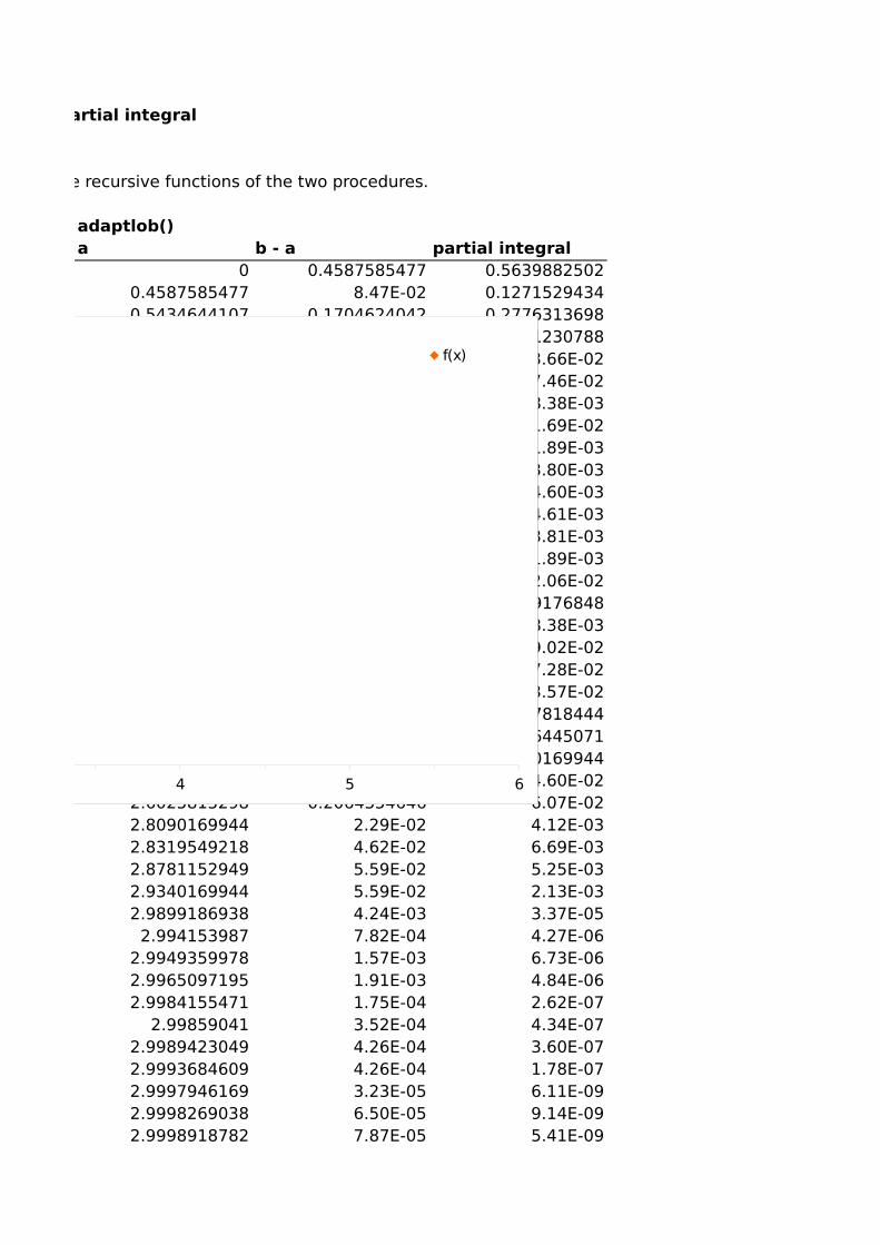
Trace the left end point of the current interval, the interval length and the partial integral
adaptlob()a b - a partial integral
0 0.4587585477 0.56398825020.4587585477 8.47E-02 0.12715294340.5434644107 0.1704624042 0.27763136980.7139268149 0.2064354646 0.37512307880.9203622795 1.89E-02 3.66E-020.9393030863 3.81E-02 7.46E-020.9774196386 4.24E-03 8.38E-030.9816549317 8.52E-03 1.69E-020.9901780519 9.47E-04 1.89E-030.9911250923 1.91E-03 3.80E-030.9930309199 2.31E-03 4.60E-030.9953389386 2.31E-03 4.61E-030.9976469572 1.91E-03 3.81E-030.9995527848 9.47E-04 1.89E-031.0004998252 1.03E-02 2.06E-021.0108215984 8.52E-03 0.01691768481.0193447186 4.24E-03 8.38E-031.0235800118 0.0461603732 9.02E-021.0697403849 3.81E-02 7.28E-021.1078569373 1.89E-02 3.57E-021.1267977441 0.1704624042 0.30478184441.2972601482 8.47E-02 0.14064450711.3819660113 1.1180339887 1.1840169944
2.5 0.1025815298 4.60E-022.6025815298 0.2064354646 6.07E-022.8090169944 2.29E-02 4.12E-032.8319549218 4.62E-02 6.69E-032.8781152949 5.59E-02 5.25E-032.9340169944 5.59E-02 2.13E-032.9899186938 4.24E-03 3.37E-05
2.994153987 7.82E-04 4.27E-062.9949359978 1.57E-03 6.73E-062.9965097195 1.91E-03 4.84E-062.9984155471 1.75E-04 2.62E-07
2.99859041 3.52E-04 4.34E-072.9989423049 4.26E-04 3.60E-072.9993684609 4.26E-04 1.78E-072.9997946169 3.23E-05 6.11E-092.9998269038 6.50E-05 9.14E-092.9998918782 7.87E-05 5.41E-09
statement in the respective recursive functions of the two procedures.
0 1 2 3 4 5 60
2
4
6
8
10
12
f(x)
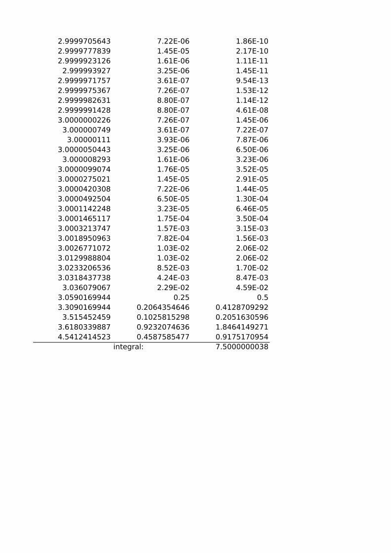
2.9999705643 7.22E-06 1.86E-102.9999777839 1.45E-05 2.17E-102.9999923126 1.61E-06 1.11E-11
2.999993927 3.25E-06 1.45E-112.9999971757 3.61E-07 9.54E-132.9999975367 7.26E-07 1.53E-122.9999982631 8.80E-07 1.14E-122.9999991428 8.80E-07 4.61E-083.0000000226 7.26E-07 1.45E-06
3.000000749 3.61E-07 7.22E-073.00000111 3.93E-06 7.87E-06
3.0000050443 3.25E-06 6.50E-063.000008293 1.61E-06 3.23E-06
3.0000099074 1.76E-05 3.52E-053.0000275021 1.45E-05 2.91E-053.0000420308 7.22E-06 1.44E-053.0000492504 6.50E-05 1.30E-043.0001142248 3.23E-05 6.46E-053.0001465117 1.75E-04 3.50E-043.0003213747 1.57E-03 3.15E-033.0018950963 7.82E-04 1.56E-033.0026771072 1.03E-02 2.06E-023.0129988804 1.03E-02 2.06E-023.0233206536 8.52E-03 1.70E-023.0318437738 4.24E-03 8.47E-03
3.036079067 2.29E-02 4.59E-023.0590169944 0.25 0.53.3090169944 0.2064354646 0.4128709292
3.515452459 0.1025815298 0.20516305963.6180339887 0.9232074636 1.84641492714.5412414523 0.4587585477 0.9175170954
integral: 7.5000000038


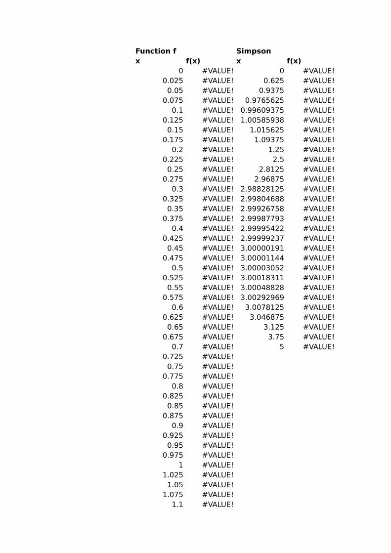
Function f Simpsonx f(x) x f(x)
0 #VALUE! 0 #VALUE!0.025 #VALUE! 0.625 #VALUE!
0.05 #VALUE! 0.9375 #VALUE!0.075 #VALUE! 0.9765625 #VALUE!
0.1 #VALUE! 0.99609375 #VALUE!0.125 #VALUE! 1.00585938 #VALUE!
0.15 #VALUE! 1.015625 #VALUE!0.175 #VALUE! 1.09375 #VALUE!
0.2 #VALUE! 1.25 #VALUE!0.225 #VALUE! 2.5 #VALUE!
0.25 #VALUE! 2.8125 #VALUE!0.275 #VALUE! 2.96875 #VALUE!
0.3 #VALUE! 2.98828125 #VALUE!0.325 #VALUE! 2.99804688 #VALUE!
0.35 #VALUE! 2.99926758 #VALUE!0.375 #VALUE! 2.99987793 #VALUE!
0.4 #VALUE! 2.99995422 #VALUE!0.425 #VALUE! 2.99999237 #VALUE!
0.45 #VALUE! 3.00000191 #VALUE!0.475 #VALUE! 3.00001144 #VALUE!
0.5 #VALUE! 3.00003052 #VALUE!0.525 #VALUE! 3.00018311 #VALUE!
0.55 #VALUE! 3.00048828 #VALUE!0.575 #VALUE! 3.00292969 #VALUE!
0.6 #VALUE! 3.0078125 #VALUE!0.625 #VALUE! 3.046875 #VALUE!
0.65 #VALUE! 3.125 #VALUE!0.675 #VALUE! 3.75 #VALUE!
0.7 #VALUE! 5 #VALUE!0.725 #VALUE!
0.75 #VALUE!0.775 #VALUE!
0.8 #VALUE!0.825 #VALUE!
0.85 #VALUE!0.875 #VALUE!
0.9 #VALUE!0.925 #VALUE!
0.95 #VALUE!0.975 #VALUE!
1 #VALUE!1.025 #VALUE!
1.05 #VALUE!1.075 #VALUE!
1.1 #VALUE!
1.125 #VALUE!1.15 #VALUE!
1.175 #VALUE!1.2 #VALUE!
1.225 #VALUE!1.25 #VALUE!
1.275 #VALUE!1.3 #VALUE!
1.325 #VALUE!1.35 #VALUE!
1.375 #VALUE!1.4 #VALUE!
1.425 #VALUE!1.45 #VALUE!
1.475 #VALUE!1.5 #VALUE!
1.525 #VALUE!1.55 #VALUE!
1.575 #VALUE!1.6 #VALUE!
1.625 #VALUE!1.65 #VALUE!
1.675 #VALUE!1.7 #VALUE!
1.725 #VALUE!1.75 #VALUE!
1.775 #VALUE!1.8 #VALUE!
1.825 #VALUE!1.85 #VALUE!
1.875 #VALUE!1.9 #VALUE!
1.925 #VALUE!1.95 #VALUE!
1.975 #VALUE!2 #VALUE!
2.025 #VALUE!2.05 #VALUE!
2.075 #VALUE!2.1 #VALUE!
2.125 #VALUE!2.15 #VALUE!
2.175 #VALUE!2.2 #VALUE!
2.225 #VALUE!2.25 #VALUE!
2.275 #VALUE!2.3 #VALUE!
2.325 #VALUE!2.35 #VALUE!
2.375 #VALUE!2.4 #VALUE!
2.425 #VALUE!2.45 #VALUE!
2.475 #VALUE!2.5 #VALUE!
2.525 #VALUE!2.55 #VALUE!
2.575 #VALUE!2.6 #VALUE!
2.625 #VALUE!2.65 #VALUE!
2.675 #VALUE!2.7 #VALUE!
2.725 #VALUE!2.75 #VALUE!
2.775 #VALUE!2.8 #VALUE!
2.825 #VALUE!2.85 #VALUE!
2.875 #VALUE!2.9 #VALUE!
2.925 #VALUE!2.95 #VALUE!
2.975 #VALUE!3 #VALUE!
3.025 #VALUE!3.05 #VALUE!
3.075 #VALUE!3.1 #VALUE!
3.125 #VALUE!3.15 #VALUE!
3.175 #VALUE!3.2 #VALUE!
3.225 #VALUE!3.25 #VALUE!
3.275 #VALUE!3.3 #VALUE!
3.325 #VALUE!3.35 #VALUE!
3.375 #VALUE!3.4 #VALUE!
3.425 #VALUE!3.45 #VALUE!
3.475 #VALUE!3.5 #VALUE!
3.525 #VALUE!3.55 #VALUE!
3.575 #VALUE!3.6 #VALUE!
3.625 #VALUE!3.65 #VALUE!
3.675 #VALUE!3.7 #VALUE!
3.725 #VALUE!3.75 #VALUE!
3.775 #VALUE!3.8 #VALUE!
3.825 #VALUE!3.85 #VALUE!
3.875 #VALUE!3.9 #VALUE!
3.925 #VALUE!3.95 #VALUE!
3.975 #VALUE!4 #VALUE!
4.025 #VALUE!4.05 #VALUE!
4.075 #VALUE!4.1 #VALUE!
4.125 #VALUE!4.15 #VALUE!
4.175 #VALUE!4.2 #VALUE!
4.225 #VALUE!4.25 #VALUE!
4.275 #VALUE!4.3 #VALUE!
4.325 #VALUE!4.35 #VALUE!
4.375 #VALUE!4.4 #VALUE!
4.425 #VALUE!4.45 #VALUE!
4.475 #VALUE!4.5 #VALUE!
4.525 #VALUE!4.55 #VALUE!
4.575 #VALUE!4.6 #VALUE!
4.625 #VALUE!4.65 #VALUE!
4.675 #VALUE!4.7 #VALUE!
4.725 #VALUE!4.75 #VALUE!
4.775 #VALUE!4.8 #VALUE!
4.825 #VALUE!4.85 #VALUE!
4.875 #VALUE!4.9 #VALUE!
4.925 #VALUE!4.95 #VALUE!
4.975 #VALUE!5 #VALUE!
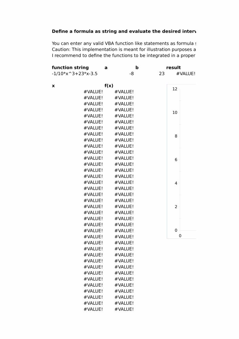
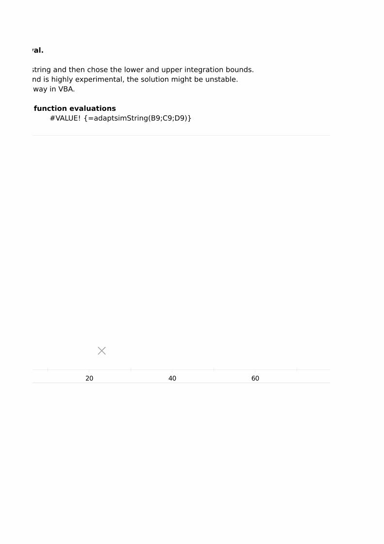
Define a formula as string and evaluate the desired interval.
You can enter any valid VBA function like statements as formula string and then chose the lower and upper integration bounds.Caution: This implementation is meant for illustration purposes and is highly experimental, the solution might be unstable.I recommend to define the functions to be integrated in a proper way in VBA.
function string a b result-1/10*x^3+23*x-3.5 -8 23 #VALUE!
x f(x)#VALUE! #VALUE!#VALUE! #VALUE!#VALUE! #VALUE!#VALUE! #VALUE!#VALUE! #VALUE!#VALUE! #VALUE!#VALUE! #VALUE!#VALUE! #VALUE!#VALUE! #VALUE!#VALUE! #VALUE!#VALUE! #VALUE!#VALUE! #VALUE!#VALUE! #VALUE!#VALUE! #VALUE!#VALUE! #VALUE!#VALUE! #VALUE!#VALUE! #VALUE!#VALUE! #VALUE!#VALUE! #VALUE!#VALUE! #VALUE!#VALUE! #VALUE!#VALUE! #VALUE!#VALUE! #VALUE!#VALUE! #VALUE!#VALUE! #VALUE!#VALUE! #VALUE!#VALUE! #VALUE!#VALUE! #VALUE!#VALUE! #VALUE!#VALUE! #VALUE!#VALUE! #VALUE!#VALUE! #VALUE!#VALUE! #VALUE!#VALUE! #VALUE!#VALUE! #VALUE!#VALUE! #VALUE!#VALUE! #VALUE!
0 20 40 60 80 100 1200
2
4
6
8
10
12
f(x)
lower

#VALUE! #VALUE!#VALUE! #VALUE!#VALUE! #VALUE!#VALUE! #VALUE!#VALUE! #VALUE!#VALUE! #VALUE!#VALUE! #VALUE!#VALUE! #VALUE!#VALUE! #VALUE!#VALUE! #VALUE!#VALUE! #VALUE!#VALUE! #VALUE!#VALUE! #VALUE!#VALUE! #VALUE!#VALUE! #VALUE!#VALUE! #VALUE!#VALUE! #VALUE!#VALUE! #VALUE!#VALUE! #VALUE!#VALUE! #VALUE!#VALUE! #VALUE!#VALUE! #VALUE!#VALUE! #VALUE!#VALUE! #VALUE!#VALUE! #VALUE!#VALUE! #VALUE!#VALUE! #VALUE!#VALUE! #VALUE!#VALUE! #VALUE!#VALUE! #VALUE!#VALUE! #VALUE!#VALUE! #VALUE!#VALUE! #VALUE!#VALUE! #VALUE!#VALUE! #VALUE!#VALUE! #VALUE!#VALUE! #VALUE!#VALUE! #VALUE!#VALUE! #VALUE!#VALUE! #VALUE!#VALUE! #VALUE!#VALUE! #VALUE!#VALUE! #VALUE!#VALUE! #VALUE!#VALUE! #VALUE!#VALUE! #VALUE!#VALUE! #VALUE!#VALUE! #VALUE!

#VALUE! #VALUE!#VALUE! #VALUE!#VALUE! #VALUE!#VALUE! #VALUE!#VALUE! #VALUE!#VALUE! #VALUE!#VALUE! #VALUE!#VALUE! #VALUE!#VALUE! #VALUE!#VALUE! #VALUE!#VALUE! #VALUE!#VALUE! #VALUE!#VALUE! #VALUE!#VALUE! #VALUE!#VALUE! #VALUE!
Define a formula as string and evaluate the desired interval.
You can enter any valid VBA function like statements as formula string and then chose the lower and upper integration bounds.Caution: This implementation is meant for illustration purposes and is highly experimental, the solution might be unstable.I recommend to define the functions to be integrated in a proper way in VBA.
function evaluations#VALUE! {=adaptsimString(B9;C9;D9)}
0 20 40 60 80 100 1200
2
4
6
8
10
12
f(x)
lower


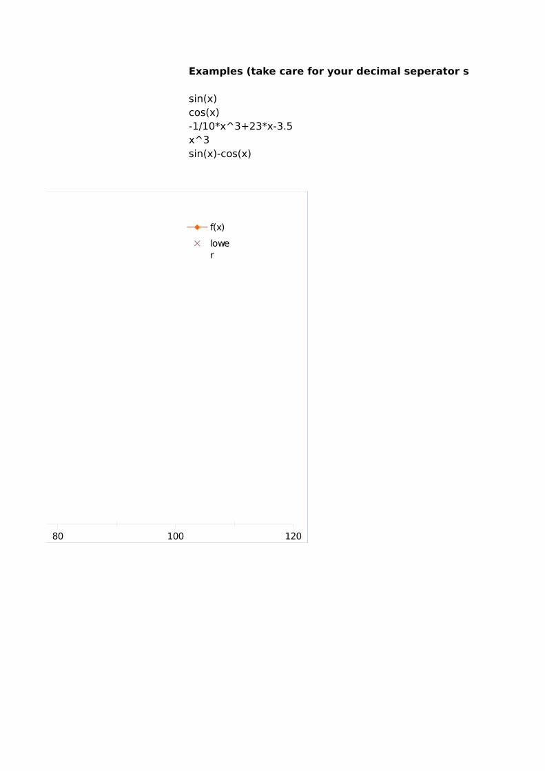
Examples (take care for your decimal seperator settings …)
sin(x)cos(x)-1/10*x^3+23*x-3.5x^3sin(x)-cos(x)
0 20 40 60 80 100 1200
2
4
6
8
10
12
f(x)
lower


Examples (take care for your decimal seperator settings …)


Disclaimer
This program is free software; you can redistribute it and/ormodify it under the terms of the GNU General Public Licenseas published by the Free Software Foundation; either version 2of the License, or (at your option) any later version.
This program is distributed in the hope that it will be useful,but WITHOUT ANY WARRANTY; without even the implied warranty ofMERCHANTABILITY or FITNESS FOR A PARTICULAR PURPOSE. See theGNU General Public License for more details.
A copy of the GNU General Public License is available athttp://www.fsf.org/licensing/licenses
Copyright © 2010 Martin Schmelzle
Contact information
[email protected]://pfadintegral.com
Revision History
Version Date By Description
1.0 2010-03-29 Martin Schmelzle Initial release