Quantum signatures of an oscillatory instability

in the Bose-Hubbard trimer

Peter Jason, Magnus Johansson and Katarina Kirr

Linköping University Post Print

N.B.: When citing this work, cite the original article.

Original Publication:

Peter Jason, Magnus Johansson and Katarina Kirr, Quantum signatures of an oscillatory

instability in the Bose-Hubbard trimer, 2012, Physical Review E. Statistical, Nonlinear, and

Soft Matter Physics, (86), 1, 016214.

http://dx.doi.org/10.1103/PhysRevE.86.016214

Copyright: American Physical Society

http://www.aps.org/

Postprint available at: Linköping University Electronic Press

http://urn.kb.se/resolve?urn=urn:nbn:se:liu:diva-79982

PHYSICAL REVIEW E 86, 016214 (2012)

Quantum signatures of an oscillatory instability in the Bose-Hubbard trimer

Peter Jason,1 Magnus Johansson,1,* and Katarina Kirr1,2

1Department of Physics, Chemistry and Biology (IFM), Linkoping University, SE-581 83 Linkoping, Sweden2Institute of Electrophysics and Radiation Technologies, 28 Chernyshevskoho Street, 61002 Kharkiv, Ukraine

(Received 5 April 2012; published 17 July 2012)

We study the Bose-Hubbard model for three sites in a symmetric, triangular configuration and search forquantum signatures of the classical regime of oscillatory instabilities, known to appear through HamiltonianHopf bifurcations for the “single-depleted-well” family of stationary states in the discrete nonlinear Schrodingerequation. In the regimes of classical stability, single quantum eigenstates with properties analogous to those ofthe classical stationary states can be identified already for rather small particle numbers. On the other hand, inthe instability regime the interaction with other eigenstates through avoided crossings leads to strong mixing,and no single eigenstate with classical-like properties can be seen. We compare the quantum dynamics resultingfrom initial conditions taken as perturbed quantum eigenstates and SU(3) coherent states, respectively, in aquantum-semiclassical transitional regime of 10–100 particles. While the perturbed quantum eigenstates do notshow a classical-like behavior in the instability regime, a coherent state behaves analogously to a perturbedclassical stationary state, and exhibits initially resonant oscillations with oscillation frequencies well describedby classical internal-mode oscillations.

DOI: 10.1103/PhysRevE.86.016214 PACS number(s): 05.45.Mt, 03.65.Sq, 03.75.Kk, 03.75.Lm

I. INTRODUCTION

Oscillatory instabilities, where a small perturbation of astationary (or time-periodic) state yields an initial oscillatorydynamics with exponentially increasing amplitude, are quiteubiquitous in the classical dynamics of Hamiltonian nonlinearlattices (see, e.g., [1] and references therein). They typicallyappear for states with inhomogeneous amplitude distribution,dividing the lattice into sublattices of sites with small and largeamplitudes, respectively, as a result of resonances betweeninternal oscillations from the different sublattices. In the linearstability problem, oscillatory instabilities arise through Hamil-tonian Hopf bifurcations yielding eigenvalues with nonzeroreal as well as imaginary parts. Well-known examples forone-dimensional lattices are, e.g., two-site localized “twisted”modes [2,3], discrete dark solitons (“dark breathers”) [4,5],spatially periodic or quasiperiodic nonlinear standing waves[6], and gap modes in diatomic chains [7,8]. In the lattercontexts, oscillatory instabilities may play an important rolein the initial stages of breather formation and thermalizationprocesses [6,8].

Arguably the simplest example of an oscillatory instabilityappears in the symmetric discrete nonlinear Schrodinger(DNLS) trimer, with f = 3 degrees of freedom interactingidentically with each other [9]. (The DNLS dimer, f = 2,is integrable and its stationary solutions may exhibit onlynonoscillatory instabilities [9].) As first discussed in [9], oneparticular family of exact stationary solutions, correspondingto two sites in antiphase oscillations and the third siteidentically zero, is oscillatorily unstable in an interval ofintermediate nonlinearity. Such solutions were later termed“single depleted well” (SDW) states [10]. The unstabledynamics, investigated in some detail in [1], involves aresonant oscillation between one mode whose main effect isto populate the empty site and another mode corresponding

*mjn@ifm.liu.se; URL: https://people.ifm.liu.se/majoh

mainly to internal population oscillations between the twononzero sites.

The DNLS model is a classical limit of the well-knownBose-Hubbard model for interacting bosons on a lattice(therefore also termed the “quantum DNLS” model [11]),when the total number of bosons N goes to infinity. Inparticular, the trimer has a direct physical application fora Bose-Einstein condensate in symmetric triple-well traps;see, e.g., [12–14] for some proposed realizations. The naturalquestion then arises: how can an oscillatory instability appearin the classical limit (“h → 0”) of a fundamental quantumlattice model?

One may consider several possible ways to characterizethe appearance of the classical oscillatory instability fromthe quantum problem, and it is the purpose of the presentwork to discuss and compare some different approaches,mainly through numerical computations for modest particlenumbers. We will characterize certain quantum signaturesof the classical instability transition, which may be experi-mentally observable as the number of bosons per lattice siteincreases.

First, we discuss the energy spectra and eigenstates forparticle number N increasing from 10 to 90. In the strong-interaction or weak-coupling (“anticontinuous”) limit thereare, for each finite (even) N , three degenerate quantumeigenstates of the form [N/2,N/2,0], with exactly zeropopulation at one of the sites. Following these states towardsweaker interaction or larger coupling, they start to mix stronglywith other states through avoided crossings in the spectrum (asseen already in [15]), and it is not a priori evident which ofthe quantum states (if any) should be considered as a quantumcounterpart to a classical single-depleted-well state. We willdiscuss various ways to characterize a “good” quantum SDWeigenstate and show that such typical “goodness” measuresdrastically decrease in an intermediate-parameter regimedominated by strong quantum resonances, which approachesthe regime of classical oscillatory instability as the particlenumber increases.

016214-11539-3755/2012/86(1)/016214(13) ©2012 American Physical Society

PETER JASON, MAGNUS JOHANSSON, AND KATARINA KIRR PHYSICAL REVIEW E 86, 016214 (2012)

We then go on to investigate the quantum dynamics forslightly perturbed quantum SDW-like eigenstates, and findthat such perturbations in general are not able to reproduce aclassical-like behavior in the instability regime.

On the other hand, it is well known (see, e.g., [12–14,16,17])that for each finite N , one may construct SU(f ) coherent states(f = 3 for a trimer), for which the time evolution obtainedfrom the Bose-Hubbard model exactly reproduces the classicalDNLS dynamics in the limit N → ∞. [The SU(f ) coherentstates are equivalent to the Hartree states of [18], but differ fromthe Glauber coherent states used, e.g., in [19,20] essentiallyin that the former conserve total particle number for any N ,while the latter conserve the rescaled particle number, theDNLS norm, only in the classical limit N → ∞.] However,even if the classical solution is an exact stationary solution(the absolute values of the coherent-state parameters are timeindependent), the corresponding coherent state will generallynot be an exact quantum eigenstate for any finite N .

Thus, since the coherent states are the most “classical-like” states but generally not eigenstates, one may look forsignatures in the properties of the finite-N coherent statesrather than the eigenstates. This is the approach used, e.g.,in [14], and may be useful in particular for large N . As weshall see, for N approaching 100 it is indeed possible to tracethe classical resonant oscillations in pure quantum dynamicsusing SU(3) coherent states as initial conditions, although thequantum instability transition for such relatively small valuesof N becomes smooth rather than sharp as in the classicalmodel.

Although, to the best of our knowledge, quantum signaturesof the classical Hamiltonian Hopf bifurcations and oscillatoryinstabilities of stationary, non-current-carrying solutions havenot been analyzed before, there are several earlier worksdiscussing quantum counterparts to other types of classicalDNLS dynamical instability transitions that deserve to bementioned in this context. For example, the classical mod-ulational instability threshold of current-carrying constant-amplitude lattice waves [21] was analyzed from the quantumBose-Hubbard perspective in [22], and in particular it wasfound that quantum fluctuations may lead to a substantialbroadening of the classical transition for a one-dimensionallattice (as we will find also for our case). Another well-studiedexample is the classical self-trapping transition, where, for anattractive effective interaction, the delocalized ground statebecomes unstable and a stable localized ground state appearsin a bifurcation [9]. The quantization of this transition, whichappears already for the dimer case f = 2, has been analyzedin a large number of papers starting from [18,23], and veryrecently in [24] (to which we also refer for a more completeset of references on this issue), where a major result is that,again, quantum fluctuations result in a critical regime ratherthan a single bifurcation point. We should, however, stress thatboth these instability transitions appear for perturbed groundstates (or highest-energy states, depending on whether theinteraction is repulsive or attractive), while Hamiltonian Hopfbifurcations necessarily must appear for excited states since thetwo resonating internal modes must contribute with differentsigns to the total energy of the stationary state (see, e.g., [1]).Thus, the physical origin of the instabilities studied here isfundamentally different from that in earlier works.

II. MODEL

The form of the Bose-Hubbard model that we will use is

HBH =3∑

i=1

{αa†i a

†i ai ai + a

†i (ai+1 + ai−1)}, (1)

with periodic boundary conditions and nonlinear parameterα > 0. Using boson commutation relations [ai ,a

†j ] = δi,j and

the number operator ni = a†i ai , this can also be written as

HBH =3∑

i=1

{αni(ni − 1) + a†i (ai+1 + ai−1)}. (2)

Following [12–14,16–18] and making an ansatz of the wavefunction as an SU(3) coherent state with a given N =∑3

i=1〈ni〉, we obtain a dynamical equation for the coherent-state parameters ai , which is the DNLS equation correspondingto the following effective classical Hamiltonian:

H=〈HBH〉=3∑

i=1

{α

(N − 1)

N|ai |4 + a∗

i (ai+1 + ai−1)

}, (3)

with∑3

i=1 |ai |2 = N . Comparing with the notation in [1],identifying C = 1

2αN

N−1 takes − 12α

NN−1 (H − 2N ) into the

classical Hamiltonian in Eq. (2) of [1].Thus, from this identification, we can conclude that

the classical condition [1,9] for oscillatory instabilityof the SDW stationary state {ai} = {√N/2, − √

N/2,0},9.077 . . . < N/C < 18, translates for a quantum SU(3) co-herent state into 4.5385 . . . /(N − 1) < α < 9/(N − 1). Onthe other hand, if one were to choose instead trial functions astensor products of standard Glauber coherent states at each site,as is done, e.g., in [19,20] (eigenfunctions of the annihilationoperators ai at each site), one would again end up with a DNLSequation for the dynamics of these coherent state parameters,but corresponding to a classical Hamiltonian without thefactor (N − 1)/N in (3). The above condition for oscillatoryinstability would then instead become 4.5385 . . . /N < α <

9/N . Clearly this distinction is irrelevant in the classical limit(assuming that α scales inversely with N to have a finite energyper particle, H/N < ∞, in this limit), and we have also foundthat the observed signatures of oscillatory instabilities for thepure quantum system (not too large N ), described below,essentially cannot determine whether one coherent-state ansatzgives a more classical-like behavior than the other. Therefore,in the remainder of this paper we will show numerical resultsusing, for convenience, αN rather than α(N − 1) as parameter[as also in Sec. IV B where SU(3) coherent states are used asinitial conditions].

Concerning the classical dynamics of perturbed SDWstates in the unstable regime, it was discovered in [1] thata self-trapping transition appears at a critical value, α ≈5.3/(N − 1) in the notation of (3). Below the transition,the unstable dynamics remains trapped close to the initialstate due to phase-space-dividing Kolmogorov-Arnold-Moser(KAM) tori, so that, although the dynamics may be weakly

016214-2

QUANTUM SIGNATURES OF AN OSCILLATORY . . . PHYSICAL REVIEW E 86, 016214 (2012)

chaotic, the amplitude of the initially unexcited site remainssmall forever. Above the transition the dynamics is stronglychaotic, and typically an intermittent population-inversiondynamics is observed with the small-amplitude oscillationmoving chaotically between all three sites. As will be seenbelow, some traces of this transition can be identified also inthe quantum model.

III. ENERGY SPECTRUM AND EIGENSTATES

We first illustrate in Fig. 1 an overall picture of the energyspectrum of Eq. (1) for particle numbers increasing fromN = 10 to N = 60. (Pictures of the general trimer spectrumfor particle numbers of this order were probably first shownin [15].)

Our initial strategy is to consider the family of exacteigenstates which approaches a state of the form [N/2,N/2,0]for large α. Due to translational invariance in the symmetrictrimer configuration (periodic boundary conditions) there arethree of these, one state with Bloch vector k = 0 and twodegenerate with k = ±2π/3; see, e.g., [11,15]. Explicitly, we

may thus use the basis states

|n1,n2,n3〉k ≡ 1√3

(|n1,n2,n3〉

+ eik|n3,n1,n2〉 + e2ik|n2,n3,n1〉). (4)

This introduces a tunneling time scale proportional to theinverse of the energy spacing between states with k = 0and k = ±2π/3 so that, close to the anticontinuous limit,an initially excited SDW state with the zero at a given sitewould in general not be an exact quantum eigenstate, butinstead we should expect the “hole” to perform periodicquantum tunnelings between all three sites. Analogously asfor single-quantum-breather states [18,25–27], we shouldexpect this tunneling time scale to go to infinity as wellin the anticontinuous as in the classical limits (properlyrescaled). Thus, for a given (rescaled) nonlinearity strengthwhere the SDW state is unstable, this should put a lowerbound on the particle number for which quantum mechanicscan properly reproduce the initial stages of an oscillatoryinstability: the tunneling frequency (energy splitting) must besmall compared to the classical oscillation frequency of theunstable eigenmode. This will be discussed further in Sec. IV.

0 5 10 15−20

0

20

40

60

80

100

120

140

α N

Ene

rgy

10 particles

0 5 10 15−50

0

50

100

150

200

250

300

α N

Ene

rgy

20 particles

0 5 10 15−50

0

50

100

150

200

250

300

350

400

450

α N

Ene

rgy

30 particles

0 5 10 15−100

0

100

200

300

400

500

600

700

800

900

α N

Ene

rgy

60 particles

FIG. 1. (Color online) Energy spectrum of Eq. (1) vs αN , for Bloch states with k = 0 and N = 10,20,30,60 particles, respectively. Thestate with the largest expansion coefficient for the basis function |N/2,N/2,0〉0 (see text) is plotted with a bold (blue) line.

016214-3

PETER JASON, MAGNUS JOHANSSON, AND KATARINA KIRR PHYSICAL REVIEW E 86, 016214 (2012)

5.8 5.9 6 6.1 6.2 6.3 6.4 6.5 6.633

34

35

36

37

38

39

40

41

α N

Ene

rgy

(i)

(ii)

(iii)

(iv)

0 20 40 60 80−0.5

0

0.5(i)

basis state number

coef

ficie

nt

0 20 40 60 80−0.5

0

0.5(ii)

basis state number

coef

ficie

nt

0 20 40 60 80−0.5

0

0.5(iii)

basis state number

coef

ficie

nt

0 20 40 60 80−0.5

0

0.5(iv)

basis state number

coef

ficie

nt

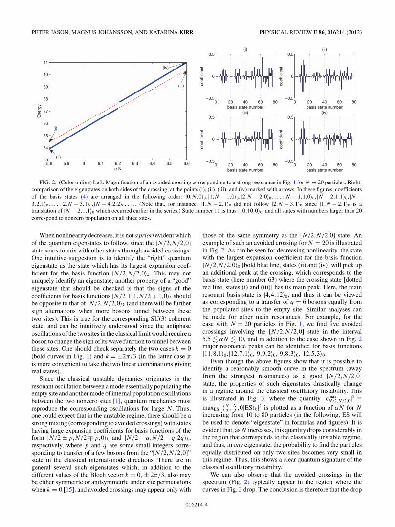
FIG. 2. (Color online) Left: Magnification of an avoided crossing corresponding to a strong resonance in Fig. 1 for N = 20 particles. Right:comparison of the eigenstates on both sides of the crossing, at the points (i), (ii), (iii), and (iv) marked with arrows. In these figures, coefficientsof the basis states (4) are arranged in the following order: |0,N,0〉0,|1,N − 1,0〉0,|2,N − 2,0〉0, . . . ,|N − 1,1,0〉0,|N − 2,1,1〉0,|N −3,2,1〉0, . . . ,|2,N − 3,1〉0,|N − 4,2,2〉0, . . . . (Note that, for instance, |1,N − 2,1〉0 did not follow |2,N − 3,1〉0 since |1,N − 2,1〉0 is atranslation of |N − 2,1,1〉0 which occurred earlier in the series.) State number 11 is thus |10,10,0〉0, and all states with numbers larger than 20correspond to nonzero population on all three sites.

When nonlinearity decreases, it is not a priori evident whichof the quantum eigenstates to follow, since the [N/2,N/2,0]state starts to mix with other states through avoided crossings.One intuitive suggestion is to identify the “right” quantumeigenstate as the state which has its largest expansion coef-ficient for the basis function |N/2,N/2,0〉k . This may notuniquely identify an eigenstate; another property of a “good”eigenstate that should be checked is that the signs of thecoefficients for basis functions |N/2 ± 1,N/2 ∓ 1,0〉k shouldbe opposite to that of |N/2,N/2,0〉k (and there will be furthersign alternations when more bosons tunnel between thesetwo sites). This is true for the corresponding SU(3) coherentstate, and can be intuitively understood since the antiphaseoscillations of the two sites in the classical limit would require aboson to change the sign of its wave function to tunnel betweenthese sites. One should check separately the two cases k = 0(bold curves in Fig. 1) and k = ±2π/3 (in the latter case itis more convenient to take the two linear combinations givingreal states).

Since the classical unstable dynamics originates in theresonant oscillation between a mode essentially populating theempty site and another mode of internal population oscillationsbetween the two nonzero sites [1], quantum mechanics mustreproduce the corresponding oscillations for large N . Thus,one could expect that in the unstable regime, there should be astrong mixing (corresponding to avoided crossings) with stateshaving large expansion coefficients for basis functions of theform |N/2 ± p,N/2 ∓ p,0〉k and |N/2 − q,N/2 − q,2q〉k ,respectively, where p and q are some small integers corre-sponding to transfer of a few bosons from the “[N/2,N/2,0]”state in the classical internal-mode directions. There are ingeneral several such eigenstates which, in addition to thedifferent values of the Bloch vector k = 0, ± 2π/3, also maybe either symmetric or antisymmetric under site permutationswhen k = 0 [15], and avoided crossings may appear only with

those of the same symmetry as the [N/2,N/2,0] state. Anexample of such an avoided crossing for N = 20 is illustratedin Fig. 2. As can be seen for decreasing nonlinearity, the statewith the largest expansion coefficient for the basis function|N/2,N/2,0〉0 [bold blue line, states (ii) and (iv)] will pick upan additional peak at the crossing, which corresponds to thebasis state (here number 63) where the crossing state [dottedred line, states (i) and (iii)] has its main peak. Here, the mainresonant basis state is |4,4,12〉0, and thus it can be viewedas corresponding to a transfer of q = 6 bosons equally fromthe populated sites to the empty site. Similar analyses canbe made for other main resonances. For example, for thecase with N = 20 particles in Fig. 1, we find five avoidedcrossings involving the [N/2,N/2,0] state in the interval5.5 � αN � 10, and in addition to the case shown in Fig. 2major resonance peaks can be identified for basis functions|11,8,1〉0,|12,7,1〉0,|9,9,2〉0,|9,8,3〉0,|12,5,3〉0.

Even though the above figures show that it is possible toidentify a reasonably smooth curve in the spectrum (awayfrom the strongest resonances) as a good [N/2,N/2,0]state, the properties of such eigenstates drastically changein a regime around the classical oscillatory instability. Thisis illustrated in Fig. 3, where the quantity |cmax

N/2,N/2,0|2 ≡maxES |〈N

2 ,N2 ,0|ES〉k|2 is plotted as a function of αN for N

increasing from 10 to 80 particles (in the following, ES willbe used to denote “eigenstate” in formulas and figures). It isevident that, as N increases, this quantity drops considerably inthe region that corresponds to the classically unstable regime,and thus, in any eigenstate, the probability to find the particlesequally distributed on only two sites becomes very small inthis regime. Thus, this shows a clear quantum signature of theclassical oscillatory instability.

We can also observe that the avoided crossings in thespectrum (Fig. 2) typically appear in the region where thecurves in Fig. 3 drop. The conclusion is therefore that the drop

016214-4

QUANTUM SIGNATURES OF AN OSCILLATORY . . . PHYSICAL REVIEW E 86, 016214 (2012)

0 5 10 150.1

0.15

0.2

0.25

0.3

0.35

0.4

0.45

0.5

αN

|cN

/2,N

/2,0

|2

10 particles

0 5 10 150.05

0.1

0.15

0.2

0.25

0.3

0.35

0.4

αN

|cN

/2,N

/2,0

|2

20 particles

0 5 10 150.05

0.1

0.15

0.2

0.25

0.3

αN

|cN

/2,N

/2,0

|2

30 particles

0 5 10 150

0.05

0.1

0.15

0.2

0.25

αN

|cN

/2,N

/2,0

|2

40 particles

0 5 10 150

0.05

0.1

0.15

0.2

0.25

αN

|cN

/2,N

/2,0

|2

50 particles

0 5 10 150

0.05

0.1

0.15

0.2

αN

|cN

/2,N

/2,0

|2

60 particles

0 5 10 150.02

0.04

0.06

0.08

0.1

0.12

0.14

0.16

0.18

αN

|cN

/2,N

/2,0

|2

70 particles

0 5 10 150.02

0.04

0.06

0.08

0.1

0.12

0.14

0.16

0.18

αN

|cN

/2,N

/2,0

|2

80 particles

FIG. 3. (Color online) The maximum probability that, in any eigenstate, all particles are equally distributed between only two sites, plottedas a function of αN for N between 10 and 80 particles. Blue (darker) and green (lighter) curves correspond to k = 0 and k = ±2π/3,respectively. The shaded region marks the classical instability regime.

in Fig. 3, and also the instability, are related to the avoidedcrossings and the mixing of eigenstates. The avoided crossingsthat, possibly, occur outside this region cannot be seen in ourplots, which means that the eigenstates would get very closeand the mixing would therefore be very swift.

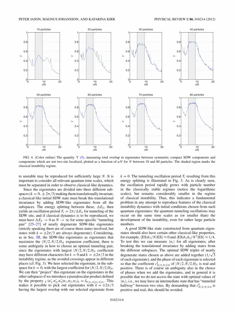
A complementary approach is to look globally rather thanlocally at the eigenspectrum, and consider a measure ofthe total overlap between symmetric “compact” SDW basisstates |N/2,N/2,0〉k and basis states which are not two-sitelocalized, as summed over all the eigenstates for a givenN . This can be considered as a necessary (but generally notsufficient) condition for development of an instability: if theoverlap is small, an initial exact zero in a SDW excitation cannever grow large. The quantity that we use to measure this“overlap” property is

ϒ ≡∑ES

∣∣∣∣⟨N

2,N

2,0|ES

⟩k

∣∣∣∣2(

1 −N−1∑n=1

|〈N − n,n,0|ES〉k|2)

.

(5)

A plot of ϒ is shown in Fig. 4. Low values of ϒ implies thateigenstates with a large portion of |N

2 ,N2 ,0〉k contain very little

of states not entirely located on two sites. They will thereforenot excite the empty site much. As is clear from Fig. 4, aplateau of high values of ϒ starts to develop as N increases (atendency can be seen already for N = 10 bosons), and alreadyfor N = 80 it corresponds almost perfectly to the classical

instability regime. Thus, this measure can also be used as aclear instability indicator here. (The increase for small α is notrelated to any instability, but reflects the general delocalizationtendency of eigenstates in the linear limit.)

IV. DYNAMICS

A number of numerical simulations of the dynamics havebeen performed, in order to elucidate to what extent thequantum dynamics, for relatively small particle numbers,may reproduce essential features of the classical SDW statetransition from stable internal-mode oscillations to oscillatoryinstability. Since there is no unique choice of quantum initialstate corresponding to the classical SDW stationary state,we will here separately discuss two alternative possibilities:slightly perturbed specific eigenstates (Sec. IV A) and SU(3)coherent states (Sec. IV B).

A. Eigenstate

The analysis in Sec. III indicates that we can generallyidentify a “quantum SDW” eigenstate, interacting resonantlywith symmetry-breaking eigenstates in the regime of classicalinstability. We may thus investigate the dynamics for a slightlyperturbed quantum SDW eigenstate by making a small,symmetry-breaking change in some expansion coefficents,and check if the classical transition from stable oscillations

016214-5

PETER JASON, MAGNUS JOHANSSON, AND KATARINA KIRR PHYSICAL REVIEW E 86, 016214 (2012)

0 10 200

0.2

0.4

0.6

0.8

1

αN

ϒ

10 particles

0 10 200

0.2

0.4

0.6

0.8

1

αN

ϒ

20 particles

0 10 200

0.2

0.4

0.6

0.8

1

αN

ϒ

30 particles

0 10 200

0.2

0.4

0.6

0.8

1

αN

ϒ

40 particles

0 10 200

0.2

0.4

0.6

0.8

1

αN

ϒ

50 particles

0 10 200

0.2

0.4

0.6

0.8

1

αN

ϒ

60 particles

0 10 200

0.2

0.4

0.6

0.8

1

αN

ϒ

70 particles

0 10 200

0.2

0.4

0.6

0.8

1

αN

ϒ

80 particles

FIG. 4. (Color online) The quantity ϒ (5), measuring total overlap in eigenstates between symmetric compact SDW components andcomponents which are not two-site localized, plotted as a function of αN for N between 10 and 80 particles. The shaded region marks theclassical instability regime.

to unstable may be reproduced for sufficiently large N . It isimportant to consider all relevant quantum time scales, whichmust be separated in order to observe classical-like dynamics.

Since the eigenstates are divided into three different sub-spaces (k = 0, ± 2π/3) making them translationally invariant,a classical-like initial SDW state must break this translationalinvariance by adding SDW-like eigenstates from all thesubspaces. The energy splitting between these, �Ek , thenyields an oscillation period Tt = 2π/�Ek for tunneling of theSDW site, and if classical dynamics is to be reproduced, wemust have �Ek → 0 as N → ∞ for some specific “tunnelingpair” [25–27] of nearly degenerate SDW-like eigenstates(strictly speaking there are of course three states involved, butstates with k = ±2π/3 are always degenerate). Considering,as in Sec. III, the SDW-like eigenstates as eigenstates thatmaximize the |N/2,N/2,0〉k expansion coefficient, there issome ambiguity in how to choose an optimal tunneling pair,since the eigenstates with largest |N/2,N/2,0〉k coefficientmay have different characters for k = 0 and k = ±2π/3 in theinstability regime, as the avoided crossings appear in differentplaces (cf. Fig. 3). We here selected the eigenstate, in the sub-space for k = 0, with the largest coefficient for |N/2,N/2,0〉0.We can then “project” this eigenstate on the eigenstates in theother subspaces if we introduce a pseudoscalar product definedby the property k′ 〈n′

1,n′2,n

′3|n1,n2,n3〉k = δn′

1n1,n′2n2,n

′3n3 . This

makes it possible to pick out eigenstates with k = ±2π/3having the largest overlap with our selected eigenstate from

k = 0. The tunneling oscillation period Tt resulting from thisenergy splitting is illustrated in Fig. 5. As is clearly seen,the oscillation period rapidly grows with particle numberin the classically stable regimes (notice the logarithmicscales), but remains considerably smaller in the regimeof classical instability. Thus, this indicates a fundamentalproblem in any attempt to reproduce features of the classicalinstability dynamics with initial conditions chosen from suchquantum eigenstates: the quantum tunneling oscillations mayoccur on the same time scales as (or smaller than) thedevelopment of the instability, even for rather large particlenumbers.

A good SDW-like state constructed from quantum eigen-states should also have certain other classical-like properties,for example, 〈ES|n3/N |ES〉≈ 0 and 〈ES|n1n2/N

2|ES〉≈ 1/4.To test this we can measure 〈ni〉 for all eigenstates, afterbreaking the translational invariance by adding states fromthe different subspaces. The optimal SDW triplet of nearlydegenerate states chosen as above are added together (1/

√3

of each eigenstate), and the phase of each eigenstate is selectedso that the coefficient ck

N/2,N/2,0 of |N/2,N/2,0〉k is real andpositive. There is of course an ambiguity also in the choiceof phases when we add the eigenstates, and in general it ispossible that we do not access the state with optimal values of〈ni〉, i.e., we may have an intermediate state that has “tunneledhalfway” between two sites. By demanding that ck

N/2,N/2,0 ispositive and real, this should be avoided.

016214-6

QUANTUM SIGNATURES OF AN OSCILLATORY . . . PHYSICAL REVIEW E 86, 016214 (2012)

0 5 10 1510

0

102

104

106

108

1010

1012

1014

60 particles

αN

Per

iod

time

20 30 40 50 60 70 80 9010

0

102

104

106

108

1010

1012

particles

Per

iod

time

αN = 10

αN = 11

αN = 12

FIG. 5. (Color online) Oscillation period Tt = 2π/�Ek corrsponding to energy splitting between the eigenstate with maximum coefficientfor the basis function |N/2,N/2,0〉0 when k = 0, and a corresponding eigenstate with k = 2π/3 as described in the text vs (left) αN forfixed N = 60 particles (the saturation around 1012 is due to using a limited numerical accuracy), and (right) particle number N for fixedαN = 10,11,12 (from bottom to top). The shaded region in the left figure marks the classical instability regime.

In Fig. 6 we show 〈ni/N〉min and 〈ninj/N2〉max, respec-

tively, for the states maximizing the |N/2,N/2,0〉0 expansioncoefficient, as a function of αN for different numbers ofparticles. From these plots it is evident that 〈ni/N〉min

(〈ninj/N2〉max) is not a strictly decreasing (increasing) func-

tion of the number of particles in the unstable region. Onthe other hand, in the classically stable regimes they wellapproach the classically expected values 0 (0.25) alreadyfor N of the order of 100 particles. Note that Fig. 6 alsoshows an interesting feature in terms of plateaus developing inthe upper part of the classical instability region. This mightbe a sign of the strongly chaotic regime, surrounding theclassical unstable SDW solution for these parameter values [1].

Note also the different behaviors around the lower and upperclassical instability thresholds: Around the lower threshold,where the classical unstable dynamics is self-trapped [1],the expectation values slowly increase (decrease) from theirclassical values until stronger resonances start to appear aroundthe self-trapping transition at αN ≈ 5.3. On the other hand, atthe upper threshold the expectation values remain nonclassicalalso in a part of the classically stable regime (9 < αN � 10for N = 100) where they only slowly approach the classicalvalues as N increases.

We also found other SDW-like candidates among the eigen-states in the classical instability regime, using the same criteriaas above (〈ES|n3/N |ES〉 ≈ 0 and 〈ES|n1n2/N

2|ES〉 ≈ 1/4).

4 5 6 7 8 9 10 11 120.1

0.15

0.2

0.25

αN

<n in j/N

2 >m

ax

6080100

4 5 6 7 8 9 10 11 120

0.05

0.1

0.15

0.2

0.25

0.3

0.35

αN

<n i/N

>m

in

6080100

FIG. 6. (Color online) 〈ni/N〉min (left) and 〈ninj /N2〉max (right) as a function of αN , for linear combinations of eigenstates with k =

0, ± 2π/3 with maximum coefficient for the basis function |N/2,N/2,0〉0, for N = 60 (dotted blue), N = 80 (light green), and N = 100 (darkred), particles. The shaded region marks the classical instability regime.

016214-7

PETER JASON, MAGNUS JOHANSSON, AND KATARINA KIRR PHYSICAL REVIEW E 86, 016214 (2012)

0 50 100 150 200−1.5

−1

−0.5

0

0.5

1

1.5

2

2.5

3x 10

−3

<n 3/N

>pe

rtur

bed−

<n 3/N

>un

pert

urbe

d

time0 50 100 150 200

0.05

0.1

0.15

0.2

0.25

0.3

0.35

0.4

0.45

time

<n 3

/N>

unpe

rtur

bed

FIG. 7. Left: Difference �〈n3/N〉 in occupation of site 3 (having initially smallest 〈ni〉) between an exact and a perturbed tunneling pairof eigenstates, prepared as described in text. Right: Dynamics over the same time range of 〈n3/N〉 for the unperturbed tunneling pair. αN = 6,N = 60.

However, these states did not show the expected antisymmetricstructure (tunneling of one particle connected with a minussign), while the eigenstate that maximizes the |N/2,N/2,0〉0

coefficient generally does (see the examples in Fig. 2, and alsoin Fig. 9 below).

We thus, first, chose as initial condition for dynamicalsimulations the linear combination of eigenstates with k = 0,

± 2π/3 with largest |N/2,N/2,0〉0 coefficient as describedabove, prepared to minimize 〈n3〉, and subsequently perturbedwith a random perturbation of the order of 1% for the expansion

0 5 10 150

0.2

0.4

0.6

0.8

1

αN

|<C

S|E

S>

|2

20 particles

0 5 10 150

0.2

0.4

0.6

0.8

1

αN

|<C

S|E

S>

|2

30 particles

0 5 10 150

0.2

0.4

0.6

0.8

1

αN

|<C

S|E

S>

|2

40 particles

0 5 10 150

0.2

0.4

0.6

0.8

1

αN

|<C

S|E

S>

|2

50 particles

0 5 10 150

0.2

0.4

0.6

0.8

1

αN

|<C

S|E

S>

|2

60 particles

0 5 10 150

0.2

0.4

0.6

0.8

1

αN

|<C

S|E

S>

|2

70 particles

0 5 10 150

0.2

0.4

0.6

0.8

1

αN

|<C

S|E

S>

|2

80 particles

0 5 10 150

0.2

0.4

0.6

0.8

190 particles

αN

|<C

S|E

S>

|2

FIG. 8. (Color online) Projection of SU(3) coherent states onto tunneling pairs of eigenstates with maximal expansion coefficient for|N/2,N/2,0〉0. Blue (dark) curves, eigenstates chosen as in Sec. IV A; green (light) curves, linear combinations of eigenstates with maximumcoefficients for |N/2,N/2,0〉k for each k. [The blue (dark) curves coincide with the green (light) curves in regimes where only the latter canbe seen.] The shaded region marks the classical instability regime.

016214-8

QUANTUM SIGNATURES OF AN OSCILLATORY . . . PHYSICAL REVIEW E 86, 016214 (2012)

0 50 100 150

−0.6

−0.4

−0.2

0

0.2

0.4

0.6

αN = 1

basis state number

coef

ficie

nt

0 50 100 150

−0.6

−0.4

−0.2

0

0.2

0.4

0.6

αN = 12

basis state number

coef

ficie

nt

0 50 100 150

−0.6

−0.4

−0.2

0

0.2

0.4

0.6

αN = 150

basis state number

coef

ficie

nt

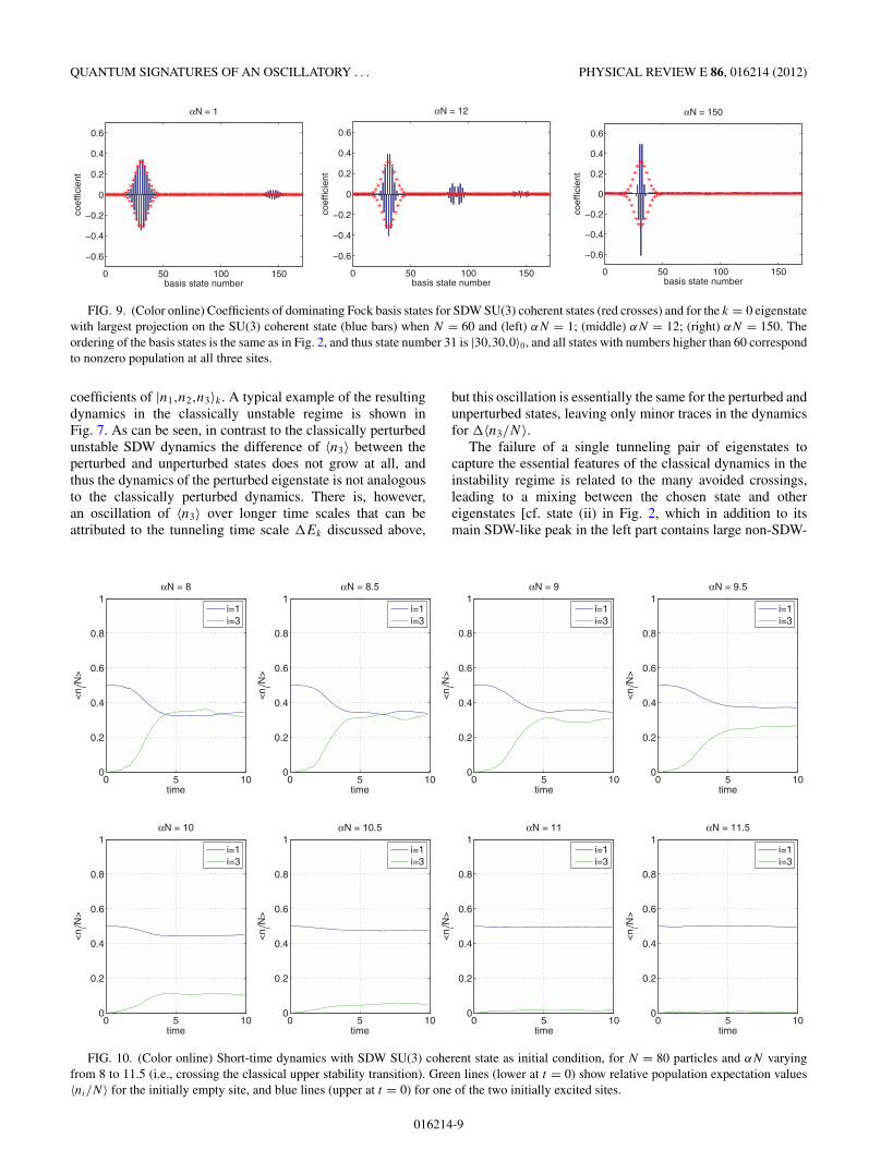
FIG. 9. (Color online) Coefficients of dominating Fock basis states for SDW SU(3) coherent states (red crosses) and for the k = 0 eigenstatewith largest projection on the SU(3) coherent state (blue bars) when N = 60 and (left) αN = 1; (middle) αN = 12; (right) αN = 150. Theordering of the basis states is the same as in Fig. 2, and thus state number 31 is |30,30,0〉0, and all states with numbers higher than 60 correspondto nonzero population at all three sites.

coefficients of |n1,n2,n3〉k . A typical example of the resultingdynamics in the classically unstable regime is shown inFig. 7. As can be seen, in contrast to the classically perturbedunstable SDW dynamics the difference of 〈n3〉 between theperturbed and unperturbed states does not grow at all, andthus the dynamics of the perturbed eigenstate is not analogousto the classically perturbed dynamics. There is, however,an oscillation of 〈n3〉 over longer time scales that can beattributed to the tunneling time scale �Ek discussed above,

but this oscillation is essentially the same for the perturbed andunperturbed states, leaving only minor traces in the dynamicsfor �〈n3/N〉.

The failure of a single tunneling pair of eigenstates tocapture the essential features of the classical dynamics in theinstability regime is related to the many avoided crossings,leading to a mixing between the chosen state and othereigenstates [cf. state (ii) in Fig. 2, which in addition to itsmain SDW-like peak in the left part contains large non-SDW-

0 5 100

0.2

0.4

0.6

0.8

1αN = 8

<n i/N

>

time

i=1i=3

0 5 100

0.2

0.4

0.6

0.8

1αN = 8.5

<n i/N

>

time

i=1i=3

0 5 100

0.2

0.4

0.6

0.8

1αN = 9

<n i/N

>

time

i=1i=3

0 5 100

0.2

0.4

0.6

0.8

1αN = 9.5

<n i/N

>

time

i=1i=3

0 5 100

0.2

0.4

0.6

0.8

1αN = 10

<n i/N

>

time

i=1i=3

0 5 100

0.2

0.4

0.6

0.8

1αN = 10.5

<n i/N

>

time

i=1i=3

0 5 100

0.2

0.4

0.6

0.8

1αN = 11

<n i/N

>

time

i=1i=3

0 5 100

0.2

0.4

0.6

0.8

1αN = 11.5

<n i/N

>

time

i=1i=3

FIG. 10. (Color online) Short-time dynamics with SDW SU(3) coherent state as initial condition, for N = 80 particles and αN varyingfrom 8 to 11.5 (i.e., crossing the classical upper stability transition). Green lines (lower at t = 0) show relative population expectation values〈ni/N〉 for the initially empty site, and blue lines (upper at t = 0) for one of the two initially excited sites.

016214-9

PETER JASON, MAGNUS JOHANSSON, AND KATARINA KIRR PHYSICAL REVIEW E 86, 016214 (2012)

like components in its tail in the right part]. Thus, in theinstability regime already the unperturbed quantum state istoo far away from a classical SDW state to reproduce theclassical instability development [e.g., 〈n3/N〉 is not eveninitially close to zero as seen from Figs. 6 and 7 (right)]. Itis therefore reasonable to assume that the SDW-like propertiesare spread out over several eigenstates and that a “satisfying”classical-like SDW state can only be created by a superpositionof many eigenstates. On the other hand, in the classically stableregimes where the expectation values in Fig. 6 are close to theclassical values, the single tunneling pair well reproduces theclassical dynamics with superposed tunneling oscillations withperiods as in Fig. 5 (cf. Fig. 13, right part, below).

B. Coherent state

An SU(3) coherent state, converging to a classical SDWstationary solution in the classical limit, can be constructedas described, e.g., in [12–14,16,17]. In particular, we may usethe explicit expansion in Fock eigenstates given in Eq. (2.16)in [14] with coherent state parameters w1 = −1,w2 = 0 toconstruct, for any given particle number N , an SU(3) coherentstate with exactly zero population on site 2, corresponding toa classical SDW state for N → ∞.

These SU(3) coherent states are generally not eigenstatesfor finite N , and to compare with results from the previoussection we plot in Fig. 8 [blue (dark) curves] the projection ofthe coherent state on the linear combination of the three nearlydegenerate eigenstates from k = 0, ± 2π/3 with the largest|N/2,N/2,0〉0 component (the eigenstate of Fig. 3), chosen

as described in Sec. IV A. We can see that the coherent statedoes not approach the eigenstates closely, especially not in theunstable region where the projection develops a pronounceddip as N increases. We should note that the coherent state thatwe use is strictly zero on the “empty” site, while the eigenstatesgenerally have probabilities for nonzero but small populationalso on this site, which becomes negligible in the classicallimit. Figure 9 shows explicit comparisons between coherentstates and the k = 0 eigenstates with highest projection onthe coherent state (which are precisely the states with largestcoefficient for the |N/2,N/2,0〉0 basis state) in regimes ofclassical stability. Note that for small αN , the population ofthe third site is the main source of discrepancy between thecoherent state and the eigenstate, while for large αN the maindiscrepancy occurs because the eigenstate narrows towardsa single peak at |N/2,N/2,0〉 when α → ∞ for fixed N ,while the width of the coherent state by definition remainsunchanged. [A similar comparison between SU(3) coherentstates and exact eigenstates was discussed for the ground stateof the Bose-Hubbard trimer in [28].]

For comparison, we also show in Fig. 8 [green (light)curves] the corresponding projection of coherent states ontoa linear combination of three eigenstates where we insteadchose independently, for each k, the eigenstates with maximumcoefficients for the basis state |N/2,N/2,0〉k . As can be seen,in the classically stable regimes the curves coincide (the choseneigenstates for k = ±2π/3 are then generally the same), whilein the classically unstable regime the green (light) curvestypically show less pronounced dips. The more pronounceddips for the blue (dark) curves are associated with the fact that,

0 2 4 6 8 100

0.005

0.01

0.015

0.02αN=11

<n 3/N

>

time

0 2 4 6 8 100

0.005

0.01αN=11.5

<n 3/N

>

time

0 2 4 6 8 100

0.005

0.01αN=12

<n 3/N

>

time

0 10 20 30 40 500

0.01

0.02

0.03αN=11

<n 3/N

>

time

0 10 20 30 40 500

2

4

6

x 10−3 αN=12

<n 3/N

>

time

0 10 20 30 40 500

1

2

3

4

5x 10

−3 αN=13

<n 3/N

>

time

FIG. 11. Early dynamics showing the expectation value for the relative population of the initially unoccupied site, for a coherent-state initialcondition with N = 80 particles. Left: dynamics for 0 < t < 10 and, from top to bottom, αN = 11,11.5,12; right: dynamics for 0 < t < 50and, from top to bottom, αN = 11,12,13.

016214-10

QUANTUM SIGNATURES OF AN OSCILLATORY . . . PHYSICAL REVIEW E 86, 016214 (2012)

close to strong resonances, the maximum overlap criterionmay select states with k = ±2π/3 whose large overlap withthe chosen k = 0 state is not primarily due to the coherentpart corresponding to zero population on the third site, butrather due to a strong incoherent tail of basis states withnonzero population on site 3 (cf. the examples in Fig. 2). It isalso interesting to note that this feature becomes particularlypronounced in a regime of αN between approximately 5.3 and9, where the classical unstable SDW solution is surrounded bystrong chaotic dynamics. On the other hand, for N of the orderof 90 particles, we see that the green (light) and blue (dark)curves in Fig. 8 essentially coincide for 4.5 � αN � 5.3,where the classical SDW solution is unstable but surroundedby KAM tori and therefore self-trapped (cf. Figs. 10 and 11of [1]).

Figure 10 shows the short-time dynamics for a systemwith 80 particles when the coherent state is used as theinitial state. We can see that, in certain aspects, it behavessimilarly to a perturbed SDW stationary state from the classicaldynamics, and in particular the transition from a self-trappedSDW dynamics in the stable regime to population mixing inthe unstable is clearly seen as αN decreases. During a shorttime period in the beginning we can observe small-amplitudeoscillations in both the stable and the unstable regions withfrequencies that agree with the internal-mode oscillationsof the classical dynamics [see, e.g., Eq. (12) and Fig. 1in Ref. [1]]. This is illustrated more clearly in Fig. 11.Since the classical SDW solution in the stable regime has

two internal oscillation modes for the amplitudes ai , for ageneric small perturbation the population 〈n3〉 = |a3|2 of theinitially unexcited site should exhibit oscillations with thesum as well as the difference of these frequencies. Taking,e.g., the explicit example αN = 12 in Fig. 11 and pluggingin the relevant numbers in the classical formula (12) of Ref.[1], we obtain oscillation periods 2π/(ω+ + ω−) ≈ 0.34 and2π/(ω+ − ω−) ≈ 1.9, which agree well with the two majoroscillations seen in Fig. 11. As αN decreases towards theinstability transition the two classical frequencies approacheach other, so that the larger oscillation period 2π/(ω+ − ω−)increases and diverges at the transition point. This tendencyis also seen in Fig. 11. Notice also from the right figuresin Fig. 11 that there is an additional modulation with periodapproximately 25. This oscillation is a pure quantum featurewith no classical analog; the period of this oscillation increaseswith N (e.g., for N = 60 we observe similar oscillations forαN = 13 but with a period of approximately 19).

It is worth observing that there is a gradual transition fromthe stable to unstable dynamics in Fig. 10, which is essentiallya quantum effect since the classical transition occurs abruptlyat the Hamiltonian Hopf bifurcation at N = 9 [1,9]. In Fig. 12we can see that for αN = 10.0 (classically stable regime) weget a dynamics that approaches the classical stable dynamicswhen we increase the particle number.

Finally, we give in Fig. 13 a comparison between thelong-time dynamics in the classically stable regime withinitial conditions given by an SU(3) coherent state and a

0 5 100

0.2

0.4

0.6

0.8

120 particles

<n i/N

>

time

i=1i=3

0 5 100

0.2

0.4

0.6

0.8

130 particles

<n i/N

>

time

i=1i=3

0 5 100

0.2

0.4

0.6

0.8

140 particles

<n i/N

>

time

i=1i=3

0 5 100

0.2

0.4

0.6

0.8

150 particles

<n i/N

>

time

i=1i=3

0 5 100

0.2

0.4

0.6

0.8

160 particles

<n i/N

>

time

i=1i=3

0 5 100

0.2

0.4

0.6

0.8

170 particles

<n i/N

>

time

i=1i=3

0 5 100

0.2

0.4

0.6

0.8

180 particles

<n i/N

>

time

i=1i=3

0 5 100

0.2

0.4

0.6

0.8

190 particles

<n i/N

>

time

i=1i=3

FIG. 12. (Color online) Dynamics for the coherent-state initial condition for 20–90 particles, respectively, for αN = 10. The same quantitiesas in Fig. 10 are plotted.

016214-11

PETER JASON, MAGNUS JOHANSSON, AND KATARINA KIRR PHYSICAL REVIEW E 86, 016214 (2012)

0 1 2 3x 104

0

0.05

0.1

0.15

0.2

0.25

0.3

0.35

0.4

0.45

0.5

<n i/N

>

time0 1 2 3

x 104

0

0.05

0.1

0.15

0.2

0.25

0.3

0.35

0.4

0.45

0.5

<n i/N

>

time

i=1i=3

i=1i=3

FIG. 13. (Color online) Long-time dynamics for a system of 60particles and αN = 11, for initial conditions given by (left) the SU(3)coherent state, and (right) a linear combination of exact eigenstatesconstituting a SDW tunneling pair as in Fig. 5, prepared to minimize〈n3(t = 0)〉 (pseudoeigenstate).

symmetry-broken SDW “pseudoeigenstate” prepared as alinear combination of k = 0 and k = ±2π/3 exact SDWeigenstates as described in Sec. IV A, respectively. In bothcases, the observed oscillation of the population expectationvalues between the sites correspond well to an oscillationperiod of the order 104, as expected from tunneling oscillations(see Fig. 5). Note that, in these oscillations, the populationsat sites 1 and 2 never drop to zero. Due to the symmetryof the initial condition, the inital hole at site 3 can only“split” symmetrically between sites 1 and 2, and after a fulloscillation period recombine again at the original site 3. Notethat, while the symmetry-broken eigenstate initially has a smallbut nonzero value of 〈n3/N〉 (cf. Figs. 6 and 9) which it returnsto almost perfectly after one oscillation period, the coherentstate has 〈n3〉 = 0 exactly at t = 0, but returns to a valuesignificantly larger than zero after one period. This, togetherwith the small superposed oscillations for the coherent state,are the main qualitative differences between the long-timedynamics of these two types of eigenstate in the classicallystable regime.

V. CONCLUSIONS

In conclusion, using the Bose-Hubbard model for atriangular configuration, we have identified a number ofquantum signatures of the classical oscillatory instabilityregime for the single-depleted-well stationary solution ofthe corresponding discrete nonlinear Schrodinger equation.Focusing on a transitional regime between strongly quantumand semiclassical behavior with particle numbers between 10and 100, some major conclusions can be drawn:

(i) The regime of classical oscillatory instability is directlyrelated to avoided crossings in the energy spectrum, and astrong mixing between a pure SDW eigenstate and other

eigenstates corresponding to resonances which populate theoriginally unoccupied site as well as breaking the originallysymmetric population of the occupied sites.

(ii) As a consequence of these resonances, we may constructseveral measures that give clear signatures of the classicallyunstable regime already for particle numbers of the order of20–30. As a particular example, we showed that the maxi-mum probability, in any eigenstate, to have particles equallydistributed between only two sites drastically decreases in theclassically unstable regime. As another measure, we calculatedthe total overlap (5) between compact SDW basis states andbasis states which are not two-site localized, summed over alleigenstates, and found a pronounced plateau developing in theclassically unstable regime.

(iii) While in the classically stable regimes a singletunneling pair of quantum eigenstates with k = 0, ± 2π/3 canbe identified as corresponding to a classical SDW stationarystate, attempts at a similar identification in the classicallyunstable regime fail to capture essential features of the classicaldynamics. For example, we showed that the dynamics resultingfrom a slightly perturbed single tunneling pair of quantumeigenstates in the unstable regime cannot reproduce thedevelopment of the oscillatory instability. Thus, the classicalunstable dynamics must be viewed as a consequence ofglobal properties of the eigenstates, rather than of individualeigenstates.

(iv) Using instead SDW SU(3) coherent states as initialconditions for the dynamics, several features of the classicaltransition from stable internal oscillations to oscillatory in-stability could be reproduced. However, while the classicaltransition appears abruptly at a given bifurcation point,the quantum transition appears gradual. Close to the upperbifurcation point on the stable side, the quantum dynamicsfor small particle numbers may signal instability with a largepopulation developing on the initially unoccupied site, but forincreasing particle numbers the classically stable dynamics isseen to be recovered.

Thus, there are a number of interesting features relatedto the quantum dynamics of SDW states and their stability-instability transitions, and we hope that the signatures thatwe have described here may be experimentally observablefor triple-well Bose-Einstein condensate configurations in thenear future. We should stress that oscillatory instabilities alsoappear for many other types of classical stationary states inthe DNLS model [1], and it would be interesting to investigateto what extent the specific quantum signatures that we havedescribed here for the SDW states are generic.

ACKNOWLEDGMENTS

M.J. is grateful to J. C. Eilbeck for being an initial source ofinspiration for this work. Financial support from the SwedishResearch Council and the Swedish Institute is gratefullyacknowledged.

[1] M. Johansson, J. Phys. A 37, 2201 (2004).[2] J. L. Marın, S. Aubry, and L. M. Florıa, Physica D 113, 283

(1998).

[3] S. Darmanyan, A. Kobyakov, and F. Lederer, JETP 86, 682(1998).

[4] M. Johansson and Yu. S. Kivshar, Phys. Rev. Lett. 82, 85 (1999).

016214-12

QUANTUM SIGNATURES OF AN OSCILLATORY . . . PHYSICAL REVIEW E 86, 016214 (2012)

[5] A. Alvarez, J. F. R. Archilla, J. Cuevas, and F. R. Romero, New.J. Phys. 4, 72 (2002).

[6] A. M. Morgante, M. Johansson, G. Kopidakis, and S. Aubry,Phys. Rev. Lett. 85, 550 (2000); Physica D 162, 53 (2002);M. Johansson, A. M. Morgante, S. Aubry, and G. Kopidakis,Eur. Phys. J. B 29, 279 (2002).

[7] A. V. Gorbach and M. Johansson, Phys. Rev. E 67, 066608(2003); Eur. Phys. J. D 29, 77 (2004).

[8] L. Kroon, M. Johansson, A. S. Kovalev, and E. Yu. Malyuta,Physica D 239, 269 (2010).

[9] J. Carr and J. C. Eilbeck, Phys. Lett. A 109, 201 (1985);J. C. Eilbeck, P. S. Lomdahl, and A. C. Scott, Physica D 16,318 (1985).

[10] R. Franzosi and V. Penna, Phys. Rev. E 67, 046227 (2003);P. Buonsante, R. Franzosi, and V. Penna, Laser Phys. 13, 537(2003).

[11] J. C. Eilbeck, in Localization and Energy Transfer in NonlinearSystems, edited by L. Vazquez, R. S. MacKay, and M. P. Zorzano(World Scientific, Hackensack, NJ, 2003), p. 177.

[12] P. Buonsante, V. Penna, and A. Vezzani, Phys. Rev. A 72, 043620(2005).

[13] C. Lee, T. J. Alexander, and Yu. S. Kivshar, Phys. Rev. Lett. 97,180408 (2006).

[14] T. F. Viscondi and K. Furuya, J. Phys. A 44, 175301 (2011).[15] S. De Filippo, M. Fusco Girard, and M. Salerno, Nonlinearity

2, 477 (1989).

[16] K. Nemoto, C. A. Holmes, G. J. Milburn, and W. J. Munro, Phys.Rev. A 63, 013604 (2000).

[17] F. Trimborn, D. Witthaut, and H. J. Korsch, Phys. Rev. A 79,013608 (2009).

[18] E. Wright, J. C. Eilbeck, M. H. Hays, P. D. Miller, and A. C.Scott, Physica D 69, 18 (1993).

[19] D. Ellinas, M. Johansson, and P. L. Christiansen, Physica D 134,126 (1999).

[20] L. Amico and V. Penna, Phys. Rev. Lett. 80, 2189 (1998).[21] Yu. S. Kivshar and M. Peyrard, Phys. Rev. A 46, 3198

(1992).[22] E. Altman, A. Polkovnikov, E. Demler, B. I. Halperin, and

M. D. Lukin, Phys. Rev. Lett. 95, 020402 (2005); A.Polkovnikov, E. Altman, E. Demler, B. I. Halperin, and M. D.Lukin, Phys. Rev. A 71, 063613 (2005).

[23] L. Bernstein, Physica D 68, 174 (1993).[24] P. Buonsante, R. Burioni, E. Vescovi, and A. Vezzani, Phys. Rev.

A 85, 043625 (2012).[25] L. Bernstein, J. C. Eilbeck, and A. C. Scott, Nonlinearity 3, 293

(1990).[26] R. A. Pinto and S. Flach, Phys. Rev. A 73, 022717 (2006).[27] R. A. Pinto and S. Flach, in Dynamical Tunneling: Theory and

Experiment, edited by S. Keshavamurthy and P. Schlagheck(Taylor & Francis, London, 2011), Chap. 14.

[28] P. Buonsante, V. Penna, and A. Vezzani, Phys. Rev. A 82, 043615(2010).

016214-13